biostatistics workshop: missing data

1

BIOSTATISTICS WORKSHOP: MISSING DATA

Sub-Saharan Africa CFAR meetingJuly 18, 2016

Durban, South Africa

Ideal World◦ All datasets would be complete◦ Everyone will have filled in all the questions correctly◦ Everyone will have sent in all their questionnaires◦ All blood samples will make their way to the lab in time◦ All genotype data will have passed QC processes◦ No one will have a diagnosis date before their birth date◦ No men would be listed as having been pregnant

◦ All researchers would have their own biostatistician to work with

2

2

Real World◦All datasets have issues (eh, no one’s perfect)◦ People skip questions ◦ Questionnaires are missing◦ We run out of blood samples◦ We have a QC process for a reason◦ Mistakes will happen

◦ My inbox is overflowing

3

Missing data is a fact of life◦ How you handle it matters◦ Need to consider the type of missingness ◦ Different methods yield biased and/or inefficient estimates

◦ There is no magic bullet◦ …other than avoiding missing data at the design stage◦ Be aboveboard about limitations of your approach

4

“All Models are Wrong, but Some are Useful”

George Box, PhD, 1919 - 2013

3

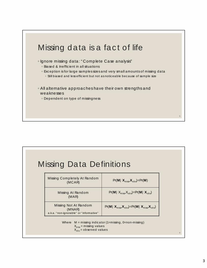
Missing data is a fact of life◦ Ignore missing data: “Complete Case analysis” ◦ Biased & Inefficient in all situations◦ Exception is for large samples sizes and very small amounts of missing data◦ Still biased and less efficient but not as noticeable because of sample size

◦ All alternative approaches have their own strengths and weaknesses◦ Dependent on type of missingness

5

Missing Data DefinitionsMissing Completely At Random

(MCAR) Pr(M|Xmiss,Xobs)=Pr(M)

Missing At Random(MAR)

Pr(M|Xmiss,Xobs)=Pr(M|Xobs)

Missing Not At Random(MNAR)

a.k.a. “non-ignorable” or “informative”

Pr(M|Xmiss,Xobs)=Pr(M|Xmiss,Xobs)

6

Where M = missing indicator (1=missing, 0=non-missing)Xmiss = missing valuesXobs = observed values

4

Missing Completely at Random (MCAR)

◦ P(M=1|Xobs, Xmiss) = P(M=1) ◦ Probability that X is missing is unrelated to the value of X or any other

covariate

◦ Dropped lab sample◦ Storm on day of clinic visit◦ 2 pages of a questionnaire stuck together◦ More?

7

Missing at Random (MAR)◦ P(M=1|Xobs , Xmiss) = P(M=1|Xobs)◦ Probability that X1 is missing is related to an OBSERVED value of another covariate X2

◦ After adjusting for the observed value X2, X1 is not associated with M

◦ Age/Income◦ Older age groups more likely to answer income question than younger age groups◦ Older age groups tend to make higher incomes◦ So overall average is inflated (if only look at non-missing)◦ Within age group. income level not related to missingness

◦ So can control for age group to deal with missingness

8

5

Missing Not at Random (MNAR)◦ P(M=1|Xobs, Xmiss) = P(M=1|Xobs, Xmiss)◦ Probability that X is missing is related to an unknown/missing value

◦ Heavy drug users are less likely to report their drug use than light users ◦ So heavy users will have more missing values and ◦ Therefore overall average will be deflated◦ So probability of missing drug use is related to higher frequencies

of use

9

Missing Data ◦ Type of missing◦ MCAR - Missing Completely at Random◦ MAR – Missing at Random◦ MNAR – Missing Not at Random

◦ There may be different types of missingness in one dataset

◦ No one method is perfect ◦ There is no one method that fits every situation

◦ So now what?

6

11

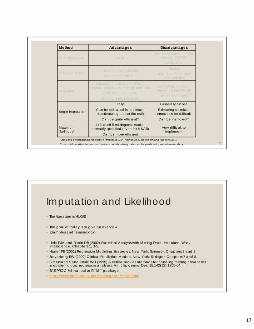
Method Advantages Disadvantages

Complete case EasyGenerally biased if data

are not MCAR*

Inefficient

Missing indicatorEasy for one variableA little more efficient

BiasedDifficult for more than

one variable

Weighted

Unbiased if data are MAR and missingness model correctly specified

Point estimation easyCan be quite efficient**

Estimating standard errors can be difficultCan be inefficient**

Single imputation

EasyCan be unbiased in important situations (e.g. under the null)

Can be quite efficient**

Generally biased Estimating standard

errors can be difficultCan be inefficient**

Maximum likelihood

Unbiased if missingness model correctly specified (even for MNAR)

Can be more efficient

Very difficult to implement

*Unbiased if missingness probability is “multiplicative” [Kleinbaum Morgenstern and Kupper (1981)]**Loss of information depends on how accurately missing data can be predicted given observed data

12



are not MCAR*

Inefficient



one variable

Weighted




Single imputation





Maximum likelihood





7

Complete Case◦ Limit dataset to only those subjects with NO missing data

◦ Issues with complete case analyses◦ Decrease sample size◦ Waste work, information, time◦ In most situations, this is biased

13

Complete Case◦ “But we will only be dropping a few, what’s the big deal?”

◦ A few here, a few there adds up fast.◦ In studies with lots of covariates… lets think◦ If we were missing only 0.5% of each X (uncorrelated)

◦ 1 outcome, 4 markers (X1, X2, X3, X4) ◦ We would expect to be missing 1.9% of our data

◦ 1 outcome, 100 markers (0.5% missing each)◦ We would expect to be missing 39% of our data

14

8

Complete Case◦ MCAR – Missingness unrelated to any known or unknown variable

◦ Unbiased◦ Loss of efficiency, especially in cases of large missingness

◦ MAR – Missing related to a measured variable◦ If related only to disease and/or exposure – as long as missingness is multiplicative then

unbiased◦ If related to some measured covariate, adjusting for covariate should elevate any most bias◦ Lose efficiency in all cases

◦ MNAR – Missing related to some unmeasured/unknown or a measured but missing variable◦ Complete Case analysis will produce biased results!

Dementia and Memory Loss in HIV◦ Ideal World: I created this dataset with n=1000 people (reality)◦ Real World: I used this ‘reality’ dataset to make 3 ‘real’ datasets with missingness

◦ MCAR – missingness is not associated with anything◦ MAR – missingness is associated with age◦ MNAR – missingness is associated with an unknown variable

◦ Collect information on◦ Score on memory test (continuous: higher is better)◦ Age (continuous)◦ Clinic ◦ Size of household (continuous)

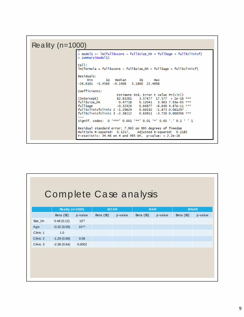
◦ Model: Linear Regression◦ Memory Score = size_hh + age + clinic

9

Reality (n=1000)

17

Complete Case analysisReality (n=1000) MCAR MAR MNAR

Beta (SE) p-value Beta (SE) p-value Beta (SE) p-value Beta (SE) p-value

Size_hh 0.48 (0.12) 10-5

Age -0.32 (0.05) 10-11

Clinic 1 1.0

Clinic 2 -1.29 (0.69) 0.06

Clinic 3 -2.38 (0.64) 0.0002

10

MCAR (n=553)

19

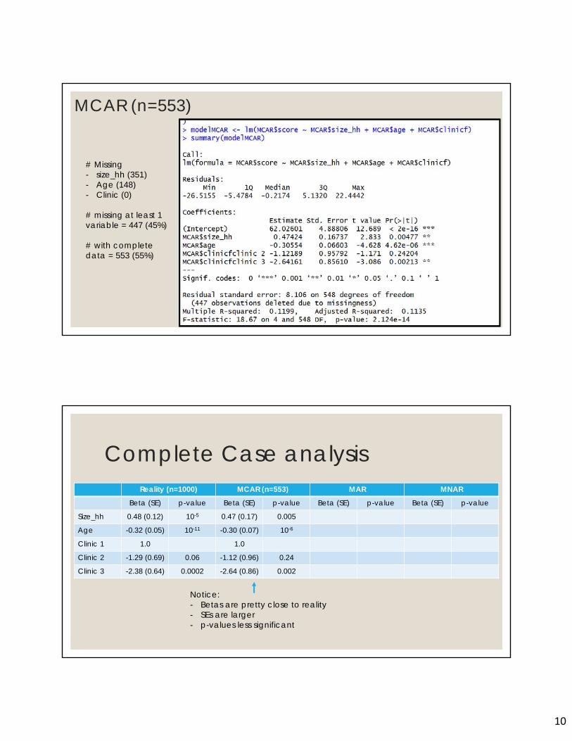
# Missing - size_hh (351)- Age (148)- Clinic (0)

# missing at least 1 variable = 447 (45%)

# with complete data = 553 (55%)

Complete Case analysisReality (n=1000) MCAR (n=553) MAR MNAR


Size_hh 0.48 (0.12) 10-5 0.47 (0.17) 0.005

Age -0.32 (0.05) 10-11 -0.30 (0.07) 10-6

Clinic 1 1.0 1.0

Clinic 2 -1.29 (0.69) 0.06 -1.12 (0.96) 0.24

Clinic 3 -2.38 (0.64) 0.0002 -2.64 (0.86) 0.002

Notice:- Betas are pretty close to reality- SEs are larger- p-values less significant

11

MAR (n=638)

21

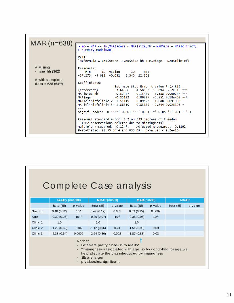
# Missing - size_hh (362)

# with complete data = 638 (64%)

Complete Case analysisReality (n=1000) MCAR (n=553) MAR (n=638) MNAR


Size_hh 0.48 (0.12) 10-5 0.47 (0.17) 0.005 0.53 (0.15) 0.0007

Age -0.32 (0.05) 10-11 -0.30 (0.07) 10-6 -0.35 (0.06) 10-8

Clinic 1 1.0 1.0 1.0

Clinic 2 -1.29 (0.69) 0.06 -1.12 (0.96) 0.24 -1.51 (0.90) 0.09

Clinic 3 -2.38 (0.64) 0.0002 -2.64 (0.86) 0.002 -1.87 (0.83) 0.03

Notice:- Betas are pretty close-ish to reality*- *missingness is associated with age, so by controlling for age we

help alleviate the bias introduced by missingness - SEs are larger- p-values less significant

12

MNAR (n=890)

23

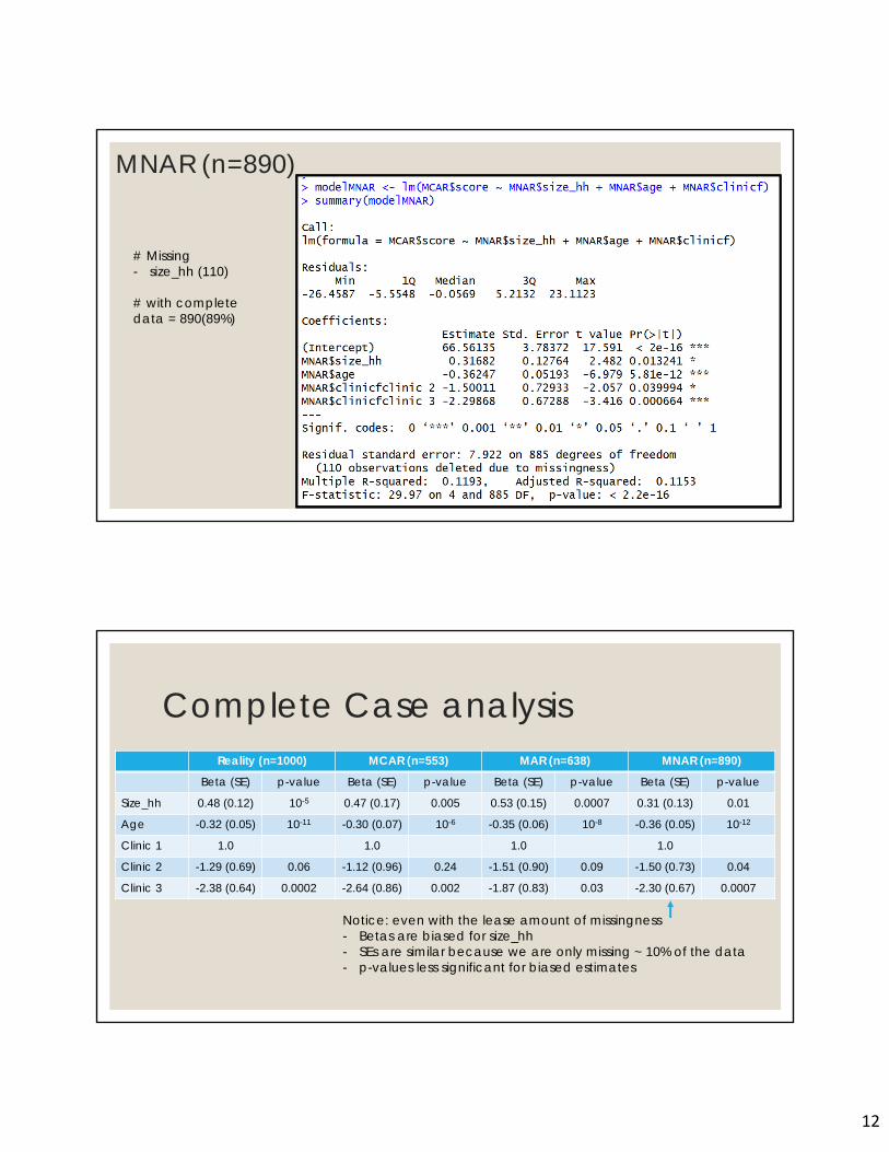
# Missing - size_hh (110)

# with complete data = 890(89%)

Complete Case analysisReality (n=1000) MCAR (n=553) MAR (n=638) MNAR (n=890)


Size_hh 0.48 (0.12) 10-5 0.47 (0.17) 0.005 0.53 (0.15) 0.0007 0.31 (0.13) 0.01

Age -0.32 (0.05) 10-11 -0.30 (0.07) 10-6 -0.35 (0.06) 10-8 -0.36 (0.05) 10-12

Clinic 1 1.0 1.0 1.0 1.0

Clinic 2 -1.29 (0.69) 0.06 -1.12 (0.96) 0.24 -1.51 (0.90) 0.09 -1.50 (0.73) 0.04

Clinic 3 -2.38 (0.64) 0.0002 -2.64 (0.86) 0.002 -1.87 (0.83) 0.03 -2.30 (0.67) 0.0007

Notice: even with the lease amount of missingness- Betas are biased for size_hh- SEs are similar because we are only missing ~ 10% of the data- p-values less significant for biased estimates

13

Summary

◦ Ok, we get it – Complete Case is bad!

◦ Complete Case:◦ Only good when little missingness AND◦ Missingness is MCAR or MAR (correctly modeled)

◦ So what can we do?

Argumentum ad antiquitatem?(proof from tradition)

“But Mom, everyone is doing it!”

26



are not MCAR*

Inefficient

Missing indicatorEasy for one categorical variable

A little more efficient


one variable

Weighted




Single imputation





Maximum likelihood





14

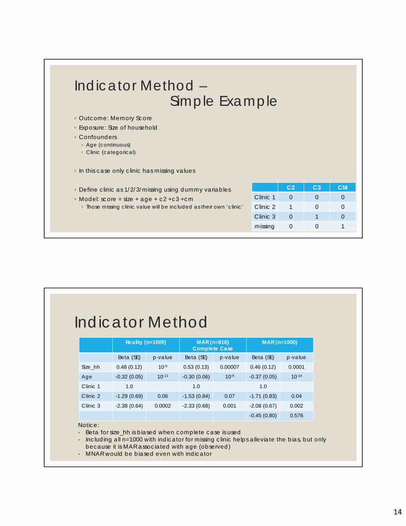
Indicator Method –Simple Example

◦ Outcome: Memory Score◦ Exposure: Size of household◦ Confounders

◦ Age (continuous)◦ Clinic (categorical)

◦ In this case only clinic has missing values

◦ Define clinic as 1/2/3/missing using dummy variables◦ Model: score = size + age + c2 +c3 +cm

◦ Those missing clinic value will be included as their own ‘clinic’

27

C2 C3 CMClinic 1 0 0 0Clinic 2 1 0 0Clinic 3 0 1 0missing 0 0 1

Indicator MethodReality (n=1000) MAR (n=818)

Complete CaseMAR (n=1000)

Beta (SE) p-value Beta (SE) p-value Beta (SE) p-value

Size_hh 0.48 (0.12) 10-5 0.53 (0.13) 0.00007 0.46 (0.12) 0.0001

Age -0.32 (0.05) 10-11 -0.30 (0.06) 10-6 -0.37 (0.05) 10-14

Clinic 1 1.0 1.0 1.0

Clinic 2 -1.29 (0.69) 0.06 -1.53 (0.84) 0.07 -1.71 (0.83) 0.04

Clinic 3 -2.38 (0.64) 0.0002 -2.33 (0.68) 0.001 -2.08 (0.67) 0.002

-0.45 (0.80) 0.576

Notice: - Beta for size_hh is biased when complete case is used- Including all n=1000 with indicator for missing clinic helps alleviate the bias, but only

because it is MAR associated with age (observed)- MNAR would be biased even with indicator

15

Indicator Method - Issues◦ For multivariate models◦ Indicator is created for every covariate, X, with any missing◦ Best used with only categorical Xs, but can make a continuous into

categorical and then make a group for missing X◦ Need to be wary◦ Look for variation in the outcome in the missing levels for each covariate◦ Need at least 1 case and 1 control for every level◦ If not, subjects missing this value must be deleted

◦ Look for ‘perfect’ missingness◦ groups of variables missing (pregnant men)◦ i.e. food frequency questionnaire◦ Can use 1 missing indicator variable

29

30



are not MCAR*

Inefficient



one variable

Weighted




Single imputation





Maximum likelihood





16

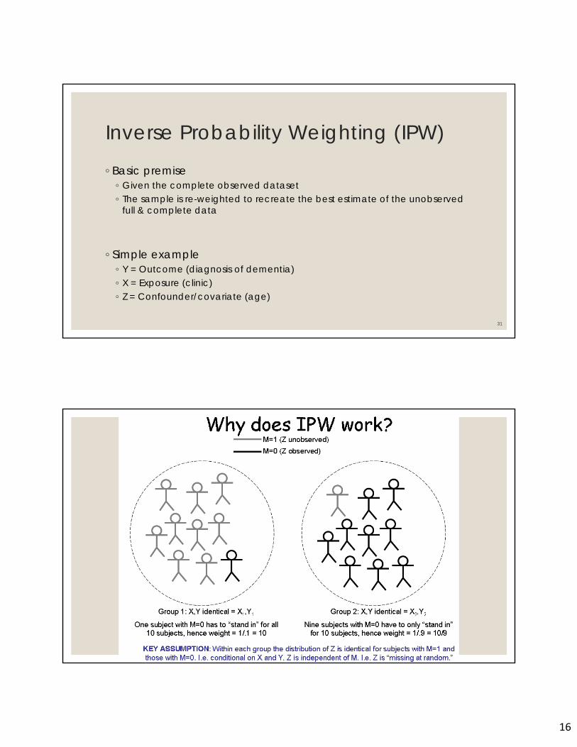
Inverse Probability Weighting (IPW)

◦ Basic premise ◦ Given the complete observed dataset◦ The sample is re-weighted to recreate the best estimate of the unobserved

full & complete data

◦ Simple example◦ Y = Outcome (diagnosis of dementia)◦ X = Exposure (clinic)◦ Z = Confounder/covariate (age)

31

17

33



are not MCAR*

Inefficient



one variable

Weighted




Single imputation





Maximum likelihood





Imputation and Likelihood◦ The literature is HUGE!

◦ The goal of today is to give an overview◦ Examples and terminology

◦ Little RJA and Rubin DB (2002) Statistical Analysis with Missing Data. Hoboken: Wiley Interscience. Chapters 1, 3-5.

◦ Harrell FE (2001) Regression Modeling Strategies. New York: Springer. Chapters 3 and 8.◦ Steyerberg EW (2009) Clinical Prediction Models. New York: Springer. Chapters 7 and 8.◦ Greenland S and Finkle WD (1995) A critical look at methods for handling missing covariates

in epidemiologic regression analyses. Am J Epidemiol Dec 15;142(12):1255-64.◦ SAS PROC MI manual or R “MI” package◦ http://www.lshtm.ac.uk/msu/missingdata/biblio.html

18

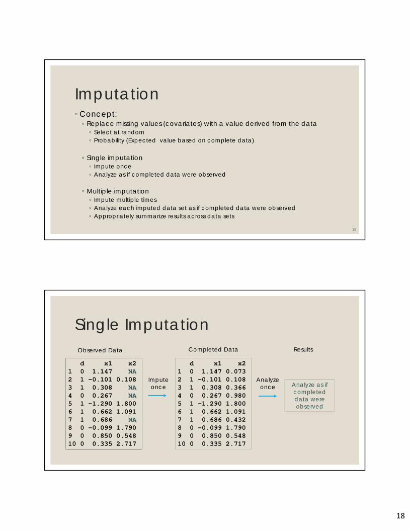
Imputation◦ Concept: ◦ Replace missing values (covariates) with a value derived from the data◦ Select at random◦ Probability (Expected value based on complete data)

◦ Single imputation◦ Impute once◦ Analyze as if completed data were observed

◦ Multiple imputation◦ Impute multiple times◦ Analyze each imputed data set as if completed data were observed◦ Appropriately summarize results across data sets

35

Single Imputation

d x1 x21 0 1.147 NA2 1 -0.101 0.1083 1 0.308 NA4 0 0.267 NA5 1 -1.290 1.8006 1 0.662 1.0917 1 0.686 NA8 0 -0.099 1.7909 0 0.850 0.54810 0 0.335 2.717

d x1 x21 0 1.147 0.0732 1 -0.101 0.1083 1 0.308 0.3664 0 0.267 0.9805 1 -1.290 1.8006 1 0.662 1.0917 1 0.686 0.4328 0 -0.099 1.7909 0 0.850 0.54810 0 0.335 2.717

Observed Data Completed Data

Analyze as if completed data were observed

Results

Impute once

Analyze once

19

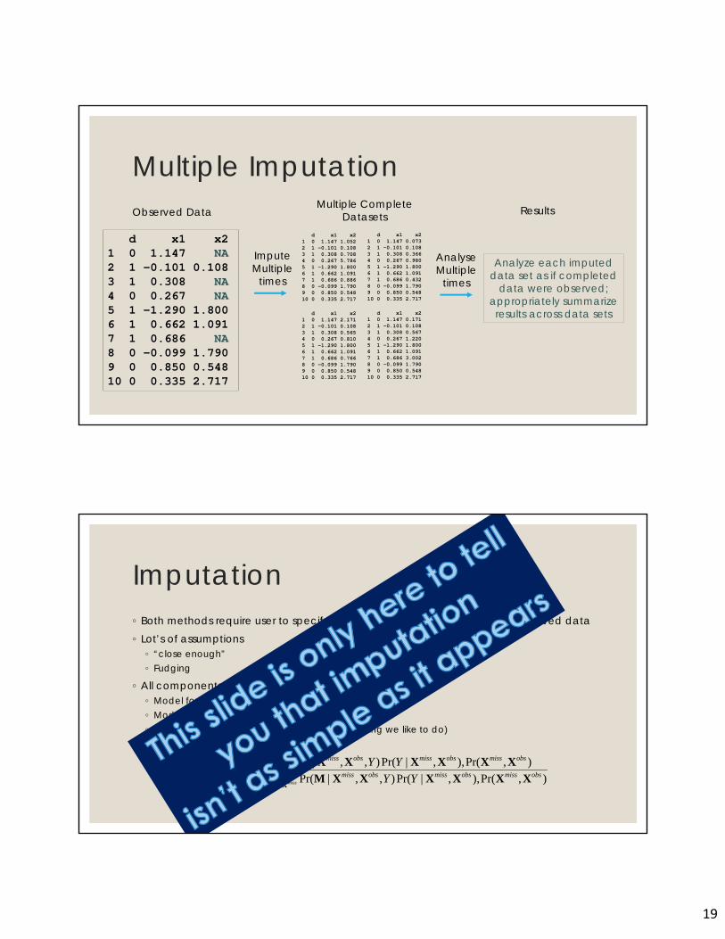
Multiple Imputation

d x1 x21 0 1.147 NA2 1 -0.101 0.1083 1 0.308 NA4 0 0.267 NA5 1 -1.290 1.8006 1 0.662 1.0917 1 0.686 NA8 0 -0.099 1.7909 0 0.850 0.54810 0 0.335 2.717

Observed DataMultiple Complete

Datasets

Analyze each imputed data set as if completed

data were observed; appropriately summarize results across data sets

Results

d x1 x21 0 1.147 1.0522 1 -0.101 0.1083 1 0.308 0.7084 0 0.267 5.7865 1 -1.290 1.8006 1 0.662 1.0917 1 0.686 0.8868 0 -0.099 1.7909 0 0.850 0.54810 0 0.335 2.717

d x1 x21 0 1.147 2.1712 1 -0.101 0.1083 1 0.308 0.5654 0 0.267 0.8105 1 -1.290 1.8006 1 0.662 1.0917 1 0.686 0.7668 0 -0.099 1.7909 0 0.850 0.54810 0 0.335 2.717

d x1 x21 0 1.147 0.0732 1 -0.101 0.1083 1 0.308 0.3664 0 0.267 0.9805 1 -1.290 1.8006 1 0.662 1.0917 1 0.686 0.4328 0 -0.099 1.7909 0 0.850 0.54810 0 0.335 2.717

d x1 x21 0 1.147 0.1712 1 -0.101 0.1083 1 0.308 0.5674 0 0.267 1.2205 1 -1.290 1.8006 1 0.662 1.0917 1 0.686 3.0028 0 -0.099 1.7909 0 0.850 0.54810 0 0.335 2.717

ImputeMultiple

times

AnalyseMultiple

times

Imputation◦ Both methods require user to specify distribution of missing values, given observed data◦ Lot’s of assumptions

◦ “close enough”◦ Fudging

◦ All components need to be specified (modeled)◦ Model for Y conditional on complete set of Xs◦ Model for Missingness ◦ Model for Joint distribution of all Xs (not something we like to do)

miss

obsmissobsmissobsmiss

obsmissobsmissobsmissobsmiss

YY

YYY

XXXXXXXM

XXXXXXMXMX

),Pr(),,|Pr(),,|Pr(

),Pr(),,|Pr(),,|Pr(),,|Pr(

20

Caveat “The idea of imputation is both seductive and

dangerous. It is seductive because it can lull the user into the pleasurable state of believing the data are complete after all, and it is dangerous because it

lumps together situations where the problem is sufficiently minor that it can be legitimately handled in this way and situations where standard estimators

applied to the real and imputed data have substantial biases.”

39

Little and Rubin pg 59

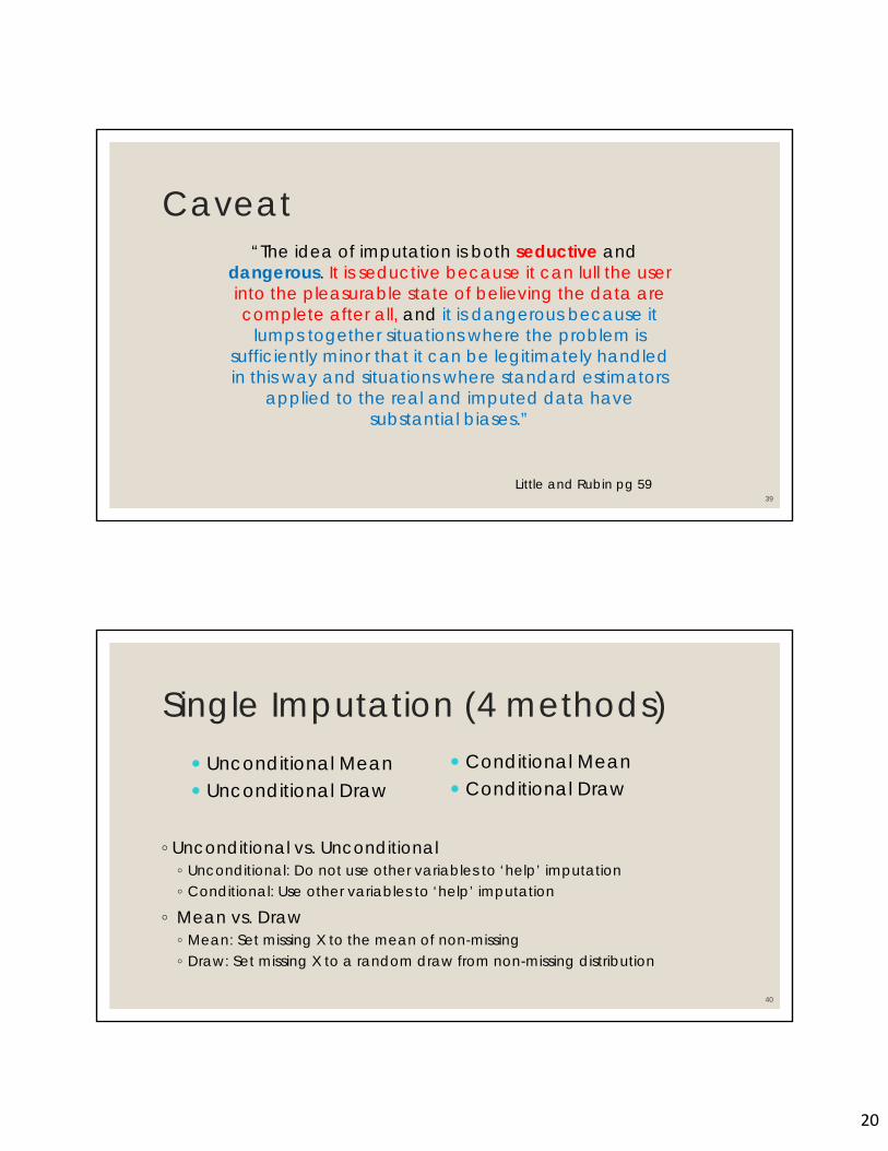
Single Imputation (4 methods)

◦ Unconditional vs. Unconditional◦ Unconditional: Do not use other variables to ‘help’ imputation◦ Conditional: Use other variables to ‘help’ imputation

◦ Mean vs. Draw◦ Mean: Set missing X to the mean of non-missing◦ Draw: Set missing X to a random draw from non-missing distribution

40

Conditional Mean Conditional Draw

Unconditional Mean Unconditional Draw

21

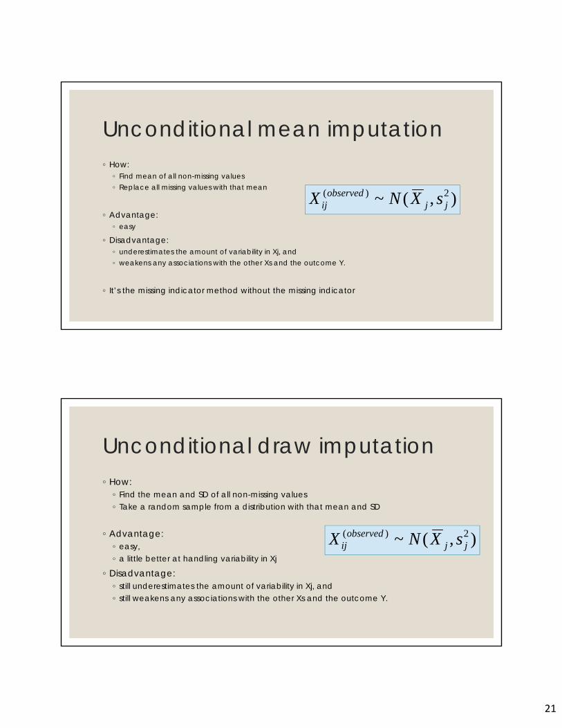
Unconditional mean imputation◦ How:

◦ Find mean of all non-missing values◦ Replace all missing values with that mean

◦ Advantage: ◦ easy

◦ Disadvantage: ◦ underestimates the amount of variability in Xj, and ◦ weakens any associations with the other Xs and the outcome Y.

◦ It’s the missing indicator method without the missing indicator

),(~ 2)(jj

observedij sXNX

Unconditional draw imputation◦ How:◦ Find the mean and SD of all non-missing values◦ Take a random sample from a distribution with that mean and SD

◦ Advantage: ◦ easy, ◦ a little better at handling variability in Xj

◦ Disadvantage: ◦ still underestimates the amount of variability in Xj, and ◦ still weakens any associations with the other Xs and the outcome Y.

),(~ 2)(jj

observedij sXNX

22

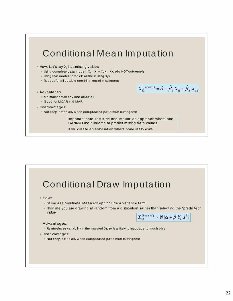
Conditional Mean Imputation

2211)(

3ˆˆˆ ii

imputedi XXX

◦ How: Let’s say X1 has missing values◦ Using complete data model: X1 = X2 + X3 +…+Xk (do NOT outcome!)◦ Using that model, ‘predict’ all the missing X1s◦ Repeat for all possible combinations of missingness

◦ Advantages:◦ Maintains efficiency (use all data)◦ Good for MCAR and MAR

◦ Disadvantages:◦ Not easy, especially when complicated patterns of missingness

Important note: this is the one imputation approach where one CANNOT use outcome to predict missing data values

It will create an association where none really exits

Conditional Draw Imputation

)ˆ,ˆˆ(~ 2)(3 sYNX iimputed

i

◦ How:◦ Same as Conditional Mean except include a variance term◦ This time you are drawing at random from a distribution, rather than selecting the ‘predicted’

value

◦ Advantages:◦ Reintroduces variability in the imputed Xs, so less likely to introduce to much bias

◦ Disadvantages:◦ Not easy, especially when complicated patterns of missingness

23

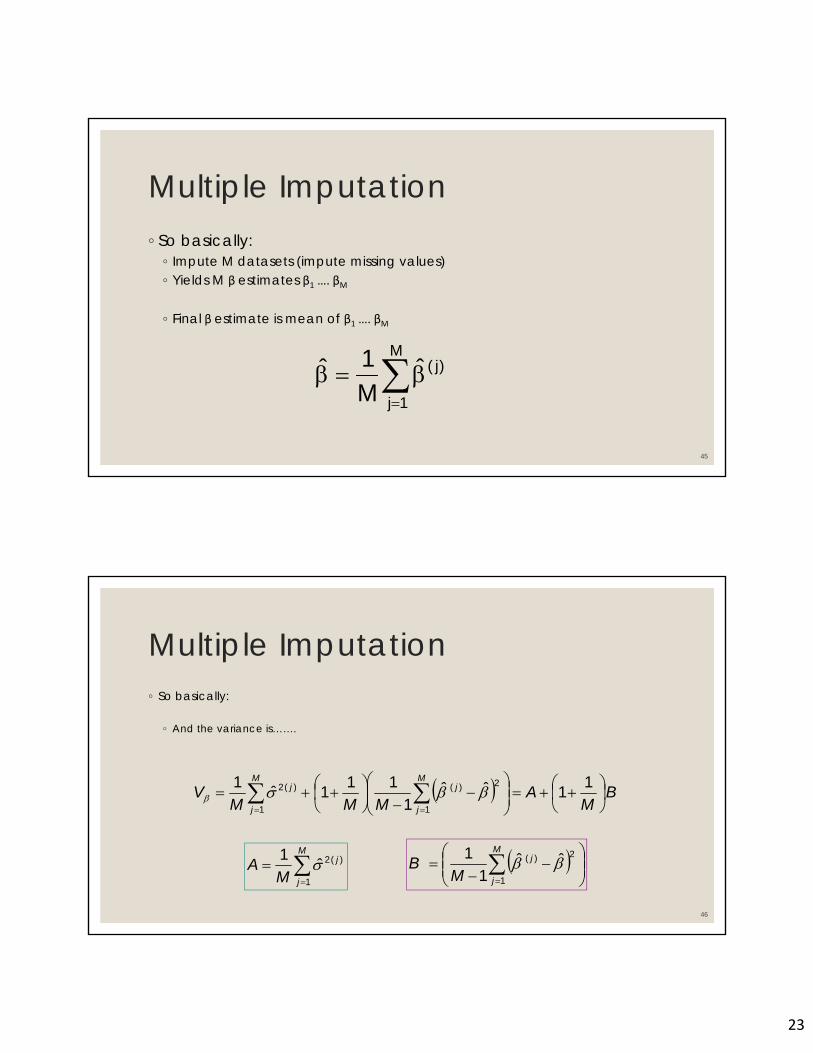
Multiple Imputation◦ So basically:◦ Impute M datasets (impute missing values)◦ Yields M β estimates β1 …. βM

◦ Final β estimate is mean of β1 …. βM

45

M

1j

)j(ˆM

1ˆ

Multiple Imputation◦ So basically:

◦ And the variance is…….

46

BM

AMMM

VM

j

jM

j

j

11ˆˆ

1

111ˆ

1

1

2)(

1

)(2

M

j

j

MA

1

)(2ˆ1

M

j

j

MB

1

2)( ˆˆ1

1

24

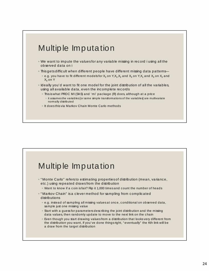
Multiple Imputation◦ We want to impute the values for any variable missing in record i using all the

observed data on i◦ This gets difficult when different people have different missing data patterns—◦ e.g. you have to fit different models for X3 on Y,X1,X2 and X3 on Y,X1 and X3 on X2 and

X3 on Y

◦ Ideally you’d want to fit one model for the joint distribution of all the variables, using all available data, even the incomplete records◦ This is what PROC MI (SAS) and ‘mi’ package (R) does, although at a price

◦ it assumes the variables [or some simple transformations of the variables] are multivariate normally distributed

◦ It does this via Markov Chain Monte Carlo methods

Multiple Imputation◦ “Monte Carlo” refers to estimating properties of distribution (mean, variance,

etc.) using repeated draws from the distribution◦ Want to know if a coin is fair? Flip it 1,000 times and count the number of heads

◦ “Markov Chain” is a clever method for sampling from complicated distributions◦ e.g. instead of sampling all missing values at once, conditional on observed data,

sample just one missing value◦ Start with a guess for parameters describing the joint distribution and the missing

data values, then randomly update to move to the next link on the chain◦ Even though you start drawing values from a distribution that looks very different from

the distribution you want, if you’ve done things right, “eventually” the Kth link will be a draw from the target distribution

25

Multiple Imputation

So far so good◦ Some analysis methods to deal with incomplete data

◦ Weighted Regressions◦ Does not replace missing values, just tries to control for it in the analysis step

◦ Imputation Techniques◦ Replaces missing value with “best guess”◦ Continuous Measures

◦ Mean & draw, conditional & unconditional◦ Single and multiple imputation

◦ Categorical Variables◦ Multiple Imputation◦ HotDeck

50

26

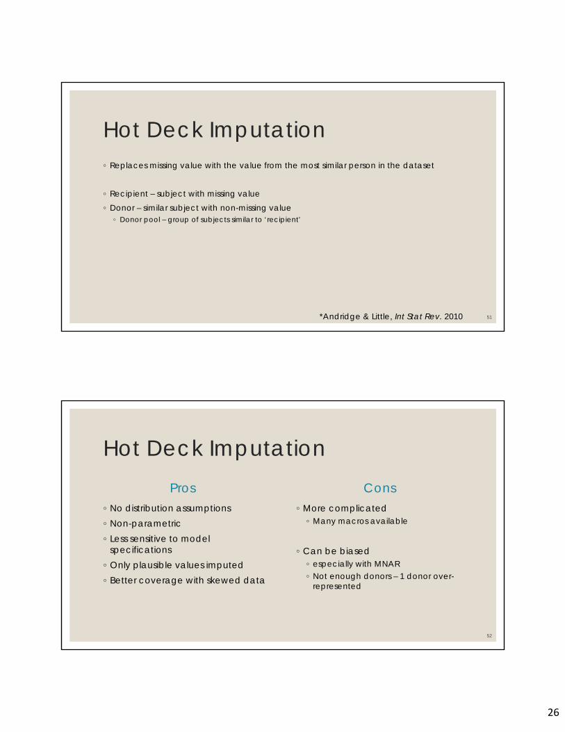
Hot Deck Imputation◦ Replaces missing value with the value from the most similar person in the dataset

◦ Recipient – subject with missing value◦ Donor – similar subject with non-missing value

◦ Donor pool – group of subjects similar to ‘recipient’

51*Andridge & Little, Int Stat Rev. 2010

Hot Deck ImputationPros

◦ No distribution assumptions◦ Non-parametric◦ Less sensitive to model

specifications◦ Only plausible values imputed◦ Better coverage with skewed data

Cons◦ More complicated ◦ Many macros available

◦ Can be biased ◦ especially with MNAR◦ Not enough donors – 1 donor over-

represented

52

27

Hot Deck Imputation◦ Replaces missing value with the value from the most similar person in the

dataset

◦ A few options:◦ Replace with 1 donor that is most similar◦ Replace with a random donor from a donor pool of similar subjects◦ Replace with mean (or other summary measure) from donor pool of similar subjects◦ Create multiple Hot Deck imputed datasets and then summarize across datasets

53

Hot Deck Imputation◦ Lots of SAS macros and R code available (google is our friend)◦ Less complicated (basically matching algorithms) to more complicated

◦ Differ based on◦ Methods (previous slide)◦ Definition of “similar”◦ Can it take into account multiple covariates◦ assumptions

54

28

Hot Deck Imputation◦ Lots of SAS macros and R packages available

◦ MIDAS: A SAS Macro for Multiple Imputation Using Distance-Aided Selection of Donors◦ R:

◦ “hot.deck”◦ “HotDeckImputation”

55

Take Away◦ It is easy to take care of missing data at the data collection stage than the data

analysis stage◦ How you deal with it will make a difference in the precision and accuracy of your

results ◦ There are multiple different methods, each with pros and cons

◦ Analysis stage: Indicator method & Weighed regression◦ Imputation: replace missing

◦ “predicted value”: conditional, unconditional, single, multiple ◦ Someone similar: HotDeck

29

QUESTIONS?

EXTRA SLIDES

30

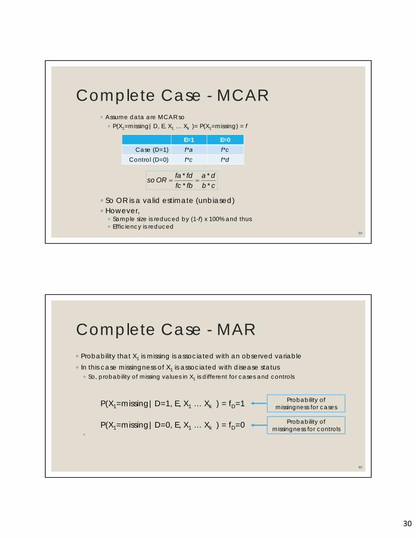
Complete Case - MCAR◦ Assume data are MCAR so◦ P(X1=missing|D, E, X1 … Xk )= P(X1=missing) = f

59

E=1 E=0Case (D=1) f*a f*c

Control (D=0) f*c f*d

cb

da

fbfc

fdfaORso

*

*

*

*

◦ So OR is a valid estimate (unbiased)◦ However,◦ Sample size is reduced by (1-f) x 100% and thus◦ Efficiency is reduced

Complete Case - MAR◦ Probability that X1 is missing is associated with an observed variable◦ In this case missingness of X1 is associated with disease status◦ So, probability of missing values in X1 is different for cases and controls

P(X1=missing|D=1, E, X1 … Xk ) = fD=1

P(X1=missing|D=0, E, X1 … Xk ) = fD=0 ◦

60

Probability of missingness for cases

Probability of missingness for controls

31

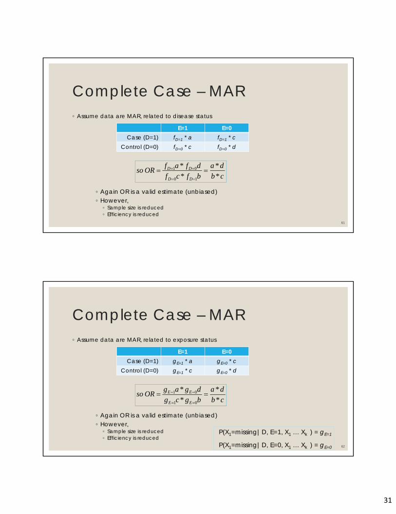
Complete Case – MAR◦ Assume data are MAR, related to disease status

61

E=1 E=0Case (D=1) fD=1 * a fD=1 * c

Control (D=0) fD=0 * c fD=0 * d

cb

da

bfcf

dfafORso

DD

DD

*

*

*

*

10

01

◦ Again OR is a valid estimate (unbiased)◦ However,

◦ Sample size is reduced ◦ Efficiency is reduced

Complete Case – MAR◦ Assume data are MAR, related to exposure status

62

E=1 E=0Case (D=1) gE=1 * a gE=0 * c

Control (D=0) gE=1 * c gE=0 * d

cb

da

bgcg

dgagORso

EE

EE

*

*

*

*

01

01

◦ Again OR is a valid estimate (unbiased)◦ However,

◦ Sample size is reduced ◦ Efficiency is reduced

P(X1=missing|D, E=1, X1 … Xk ) = gE=1

P(X1=missing|D, E=0, X1 … Xk ) = gE=0

32

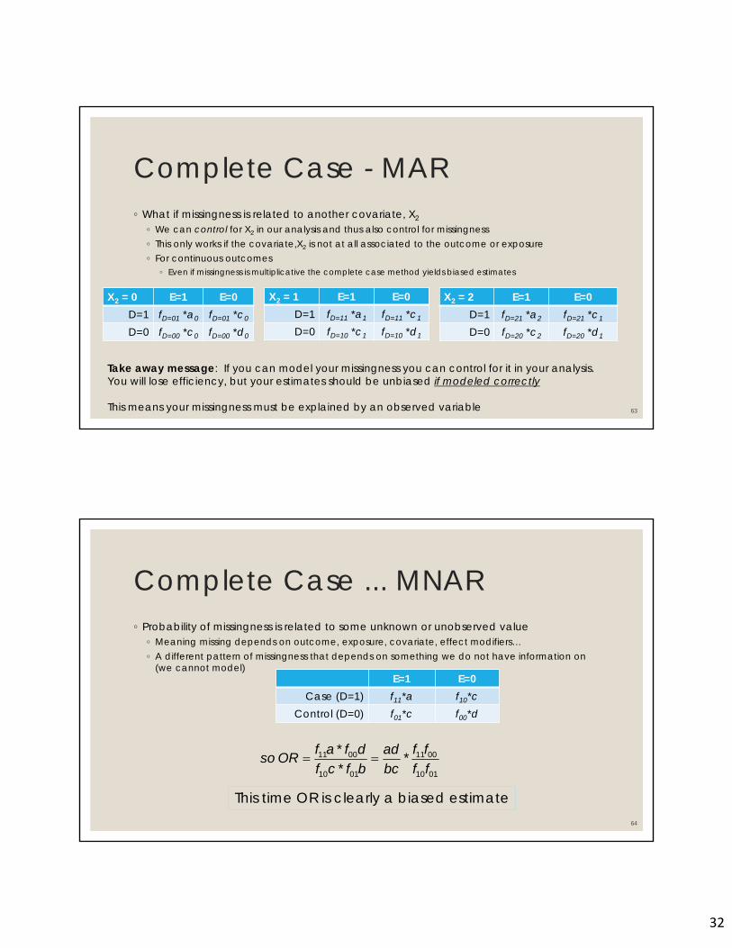
Complete Case - MAR◦ What if missingness is related to another covariate, X2

◦ We can control for X2 in our analysis and thus also control for missingness◦ This only works if the covariate,X2 is not at all associated to the outcome or exposure ◦ For continuous outcomes

◦ Even if missingness is multiplicative the complete case method yields biased estimates

63

X2 = 0 E=1 E=0D=1 fD=01 *a0 fD=01 *c0

D=0 fD=00 *c0 fD=00 *d0

X2 = 1 E=1 E=0D=1 fD=11 *a1 fD=11 *c1

D=0 fD=10 *c1 fD=10 *d1

X2 = 2 E=1 E=0D=1 fD=21 *a2 fD=21 *c1

D=0 fD=20 *c2 fD=20 *d1

Take away message: If you can model your missingness you can control for it in your analysis. You will lose efficiency, but your estimates should be unbiased if modeled correctly

This means your missingness must be explained by an observed variable

Complete Case ... MNAR◦ Probability of missingness is related to some unknown or unobserved value

◦ Meaning missing depends on outcome, exposure, covariate, effect modifiers…◦ A different pattern of missingness that depends on something we do not have information on

(we cannot model)

64

E=1 E=0Case (D=1) f11*a f10*c

Control (D=0) f01*c f00*d

0110

0011

0110

0011 **

*

ff

ff

bc

ad

bfcf

dfafORso

This time OR is clearly a biased estimate

33

65

biostatistics workshop: missing data

Health & Medicine