biostat/stat551, statistical genetics ii: quantitative...

BIOSTAT/STAT551, Statistical Genetics II: Quantitative Traits Winter 2004 Detecting Major Genes Handout 4

1

Reading: Chapter 13 and Jarvik GP (1998) Complex segregation analyses: uses and limitations. Am J Hum Genet 63:942-946. There are a number of reasons why there is interest in the detection of major genes. For us, the two most relevant are: • the potential to isolate and characterize genes influencing our trait of interest

(whether good or bad) • to be able to adjust for these since a good deal of quantitative genetic theory

assumes that a trait is influenced by many genes of small effect There are various methods available that test for the presence of a major gene: • for populations in which controlled breeding is possible • methods that rely on departure from normality to indicate the presence of a major

gene • methods that are based on resemblance between parents and offspring: Bartlett’s

test, Fain’s test, Major-gene Indices (MGI) Of greater interest to us will be • mixture models (does not take into account relatedness of individuals) • complex segregation analysis (used for data consisting of pedigrees) Mixture Models and Commingling Analysis In general, we can write the distribution of a trait that is a mixture of n underlying distributions as:


2

It is usual to assume that the population is in Hardy-Weinberg equilibrium at the major locus and that the variances across the underlying distributions are equal. For a diallelic locus that gives us a likelihood for individual i of: and a full likelihood of Maximum likelihood estimates can then be found for the 5 parameters. Testing for Specific Modes of Inheritance The likelihood ratio test can be used to test between various hypotheses: where Lr corresponds to the likelihood function for which r parameters from the full model have been assigned values. If the null hypothesis is not nested within the alternative hypothesis, then the large-sample distribution of the LRT statistic is not necessarily distributed chi-squared. One method for comparing nonnested hypotheses is Akaike’s information content (AIC) where the model with the smallest AIC is preferable:


3

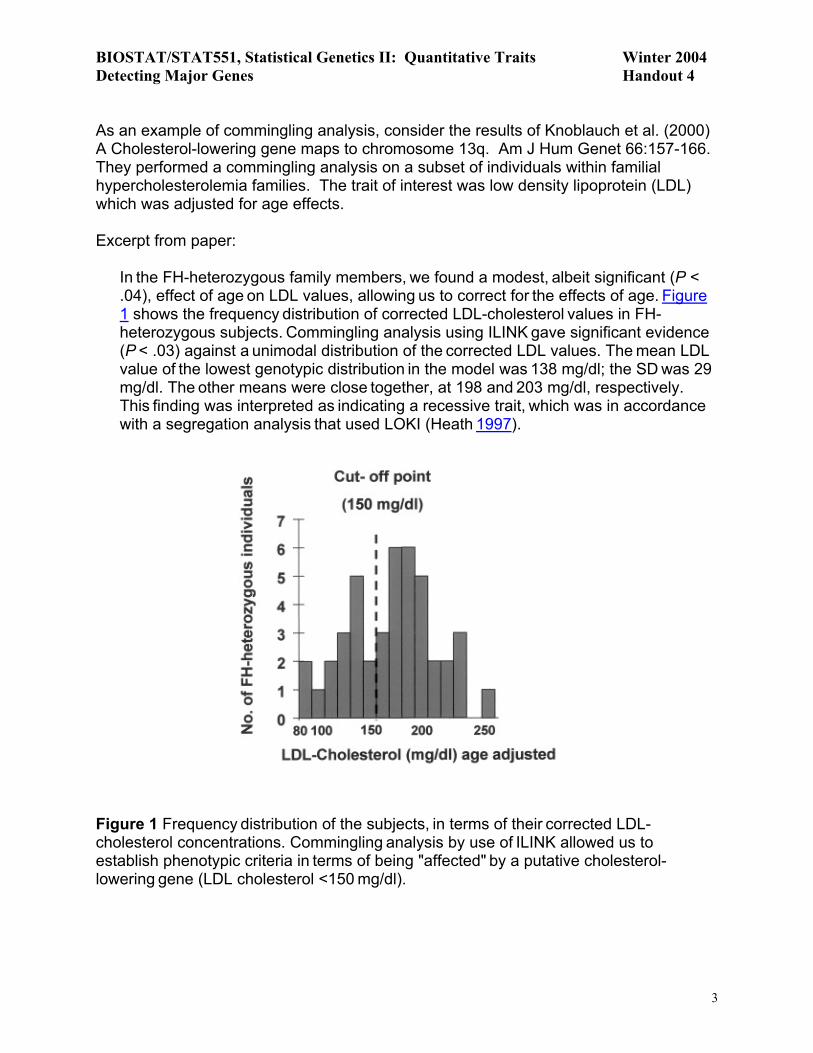
As an example of commingling analysis, consider the results of Knoblauch et al. (2000) A Cholesterol-lowering gene maps to chromosome 13q. Am J Hum Genet 66:157-166. They performed a commingling analysis on a subset of individuals within familial hypercholesterolemia families. The trait of interest was low density lipoprotein (LDL) which was adjusted for age effects. Excerpt from paper:

In the FH-heterozygous family members, we found a modest, albeit significant (P <

.04), effect of age on LDL values, allowing us to correct for the effects of age. Figure 1 shows the frequency distribution of corrected LDL-cholesterol values in FH-heterozygous subjects. Commingling analysis using ILINK gave significant evidence (P < .03) against a unimodal distribution of the corrected LDL values. The mean LDL value of the lowest genotypic distribution in the model was 138 mg/dl; the SD was 29 mg/dl. The other means were close together, at 198 and 203 mg/dl, respectively. This finding was interpreted as indicating a recessive trait, which was in accordance

with a segregation analysis that used LOKI (Heath 1997).

Figure 1 Frequency distribution of the subjects, in terms of their corrected LDL-cholesterol concentrations. Commingling analysis by use of ILINK allowed us to

establish phenotypic criteria in terms of being "affected" by a putative cholesterol-lowering gene (LDL cholesterol <150 mg/dl).


4

Problems with Non-normality Non-normality can be accommodated within the likelihood function through the use of the Box-Cox transformation: with each of the underlying distributions having a maximum of 3 parameters. This allows us to test for whether an observed skewed distribution results from • a single naturally skewed distribution • a mixture of underlying normals • a mixture of underlying distributions that can be transformed to normality


5

Modeling skewness Given

z = observed phenotype, i.e. observed trait value the distribution of z WITHIN each of the genotypic classes can be transformed to a normal distribution through the use of the Box-Cox transformation: For our scenario, it could be assumed that the individual distributions have the same transformation. That is, Let us suppose that we can find the correct transformation. The distribution on the transformed scale is then: If we assume that the observed phenotypic distribution is such that 0<y<∞ then


6

Our full likelihood is then which represents a mixture of three distributions that have separate means, but the same variance and transformation parameter. It would obviously be possible to extend this such that you allow for unequal variances or unequal transformation parameters. The program NOCOM does not allow for different transformation parameters but can allow for separate variances (although it is not recommended). More operational characteristics can be found at: http://linkage.rockefeller.edu/ott/nocom.htm The NOCOM program was originally introduced in the following article:

Ott J (1979) Detection of rare major genes in lipid levels. Hum Genet 51:79-91

They used the program to analyze the distribution of triglycerides for 991 unrelated men in the Seattle area. Their results follow:

They had reason to believe that triglycerides were distributed log-normal within each sub-distribution (one distribution or more). From their results, what would conclusions would you draw concerning the underlying genetics of triglycerides? Final words on commingling analysis • the trait distribution could be skewed due to non-genetic reasons • it is hard to distinguish a skewed distribution from a mixture of normals • if we had a mixture of a number of different skewed distributions, then by assuming

a mixture of normals our modeling will be incorrect and so we might expect a loss in power to detect commingling


7

Through our discussion of commingling analysis, we assumed that we had a sample of n random (unrelated) individuals. This gave us a likelihood that was the product over the phenotypic distribution for these n individuals.

Obviously, if our sample contains related individuals, then this likelihood will no longer be correct as related individuals will have correlated trait values (recall the information that we covered in Chapter 7). IN ADDITION, through the use of related individuals, we would expect to have increased power to detect a major gene due to the extra information given by transmissions from parents to offspring.

The extension of the simple mixture model of commingling analysis to the use of pedigree information is known as . . . Complex Segregation Analysis Consider a diallelic QTL locus with alleles Q and q. Genotypes are encoded by

=

qqforQqforQQfor

g321

For the ith family, we have The likelihood for the jth offspring of the ith family CONDITIONAL on the parent’s genotypes is: It is important to note that g represents the genotype AT THE QTL which we cannot actually measure. Also, note that this is NOT THE SAME AS LOOKING AT A MARKER.

gf gm

go


8

Example 4.1: What is the likelihood for an individual with (Qq, Qq) parents if we assume Mendelian segregation at the QTL? Thus for the ith family we have the CONDITIONAL likelihood: Recall, that the parental genotypes are unknown and so we must sum over all possible parental genotypes. This gives us the UNCONDITIONAL likelihood: If it is assumed that the QTL is in Hardy-Weinberg Equilibrium, then the frequencies for the parental genotypes can be written as our well-known functions of p=Pr(Q). The overall likelihood is then a function of five unknown parameters: To lead to a more robust approach, it was suggested by Elston et al. (1975) that Pr(go | gm, gf) be modeled as unknown parameters: τx=Pr(genotype x transmits a Q allele) Example 4.2: Given these additional parameters, what is the conditional likelihood for the trait value of a child given (Qq,QQ) parents?


9

In order to feel strongly about the presence of a major-gene, it is recommended that 1. there is a significantly better overall fit of a mixture model compared with a single

normal 2. the hypothesis of Mendelian segregation is NOT rejected 3. while the hypothesis of equal transmission for all genotypes is rejected 1⇒ 2⇒ 3⇒ In addition to the genetic effects due to the major locus, polygenic background can be added to the model. This is done by assuming the background polygenes are completely additive and that the background genetic value A is normally distributed with mean 0 and variance 2

Aσ .


10

Example 4.3: The following table is from a segregation analysis of Radiosensitivity. It can be found in Roberts SA (1999) Heritability of cellular radiosensitivity: a marker of low-penetrance predisposition genes in breast cancer? Am J Hum Genet 65: 784-794 Table 3: Model Parameters from Segregation Analysis of G2 Radiosensitivity in 20 Families

Model 1: General Transmission and Polygenes

Model 2: Major-Gene Only

Model 3: Sporadic

Model 4: Polygene Only

Model 5: Major-Environmental Only

Model 6: Major Gene + Polygene

Model 7: Major-Gene-Only, Non-Mendelian

Model 8: General-Transmission Only

Allele frequency, p

.96 .96 NA NA .77 .96 .98 .94

Means:

nn 4.48 4.48 4.63 4.67 4.48 4.48 4.48 4.47 ns 4.85 4.85 NA NA 4.81 4.84 4.85 4.81 ss 5.27 5.27 NA NA 5.17 5.30 5.28 5.18 Residual SD

.101 .101 .23 .21 .077 .10 .10 .077

Polygene heritability, H

0a [0] NA .79 [0] .30 [0] [0]

Genotype-transmission probabilities:b

1 .96 [1] NA NA [p] [1] [1] .96 2 .37 [.5] NA NA [p] [.5] .35 .37 3 .29 [0] NA NA [p] [0] [0] .29 2 × Log likelihood

76.6 68.5 9.8 18.1 50.8 71.2 71.4 76.6

No. of fitted parameters

9 5 2 3 5 6 6 8

Likelihood-ratio 2-test P values:

Compared with model 1

NA .090 <.001

<.001 <.001 .15 .16 1.0

Compared with model 2

.090 NA <.001

NA NA .11 .087 .045

NOTE.NA = not applicable. Parameters in square brackets were held fixed in the model. a Fitted parameter value at its lowest boundary. b 1, 2, and 3 take values of 1, .5, and 0, respectively, for Mendelian inheritance (see Subjects and Methods).


11

Other extensions of CSA CSA has been extended in several ways. A good review is given in the following paper:

Jarvik GP (1998) Complex segregation analyses: uses and limitations. Am J Hum Genet 63:942-946

CSA has been extended to allow for:

• multivariate traits • genotype × environment interaction • general pedigrees • various computational procedures for the likelihood function • nonrandom ascertainment

Complex Segregation Analysis of Discrete Characters Consider a dichotomous trait which is coded as follows:

diseasednormal

y

=10

Define the penetrance, ψg, of a genotype to be the probability that an individual with genotype g is diseased:

ψg=Pr( y=1 | g). The likelihood function for the trait of an individual with genotype g is then:

=)|( gyl

Arguments for constructing the likelihood for traits measured on a collection of siblings are the same as for a continuous trait. The conditional likelihood for a child’s trait given their parental genotypes is:

=),|( fm ggyl


12

The unconditional likelihood is then:

=)(yl

A polygenic background can also be added to the model. This can be done first by allowing the penetrance to be a function of the polygenic backround, ψ(g, A). The likelihood for an individual’s trait given their genotype, g, and polygenetic background, A, is then:

=),|( Agyl

This can be used to compute the likelihood for a child’ trait conditional on their parental genotypes and polygenic backgrounds:

=),,,|( fmfm AAggyl


13

Relating a discrete and quantitative traits

The penetrance functions, ψ(g, A), can be modeled assuming an underlying LIABILITY MODEL. For instance, suppose disease occurs once the liability exceeds some threshold T. The normal condition then corresponds to individuals with liability under T:

∫∞

+=

>=

TG dzAz

AgTzAg

)1,;(

),|Pr(),(

µϕ

ψ

Defining the cumulative distribution function for a unit normal U as )Pr()( xUx <=Φ then: Example 4.4: Use this relationship to write the likelihood for a child’s trait value conditional on their parental genotypes being gm=1 and gf=2.

That is, derive ).,,2,1|( fmfm AAggy ==l

More information regarding threshold characters is given in Chapter 25.


14

Before we move on to methods for linkage analysis of quantitative traits, we’re going to cover a type of aggregation/segregation analysis for dichotomous traits that relies heavily on the biometrical model. The biometrical model corresponds to Fisher’s decomposition of the genotypic value using least squares to fit additive effects for each allele with dominance effects being the residuals to this fit. The following reference for this material has been placed in the class file:

Risch N (1990) Linkage strategies for genetically complex traits. I. Multilocus models. Am J Hum Genet 46:222-228

Recurrence risk of disease in relatives The relative risk ratio represents the increased risk of disease given an individual is related to a diseased person. This is often denoted by λR and is equal to:

)individual dPr(disease)individual diseased | diseased is R typeof relativePr(

=Rλ

The numerator is often called the relative recurrence risk. − We will use the biometrical model to develop a general framework for computing the

relative recurrence risk of disease as a function of the underlying genetic parameters and the relative type.

− This framework has proven useful for studying patterns of risk across relatives as an

indicator for the underlying mode of inheritance. In particular, it has proved useful for separating additive and multiplicative risk models.


15

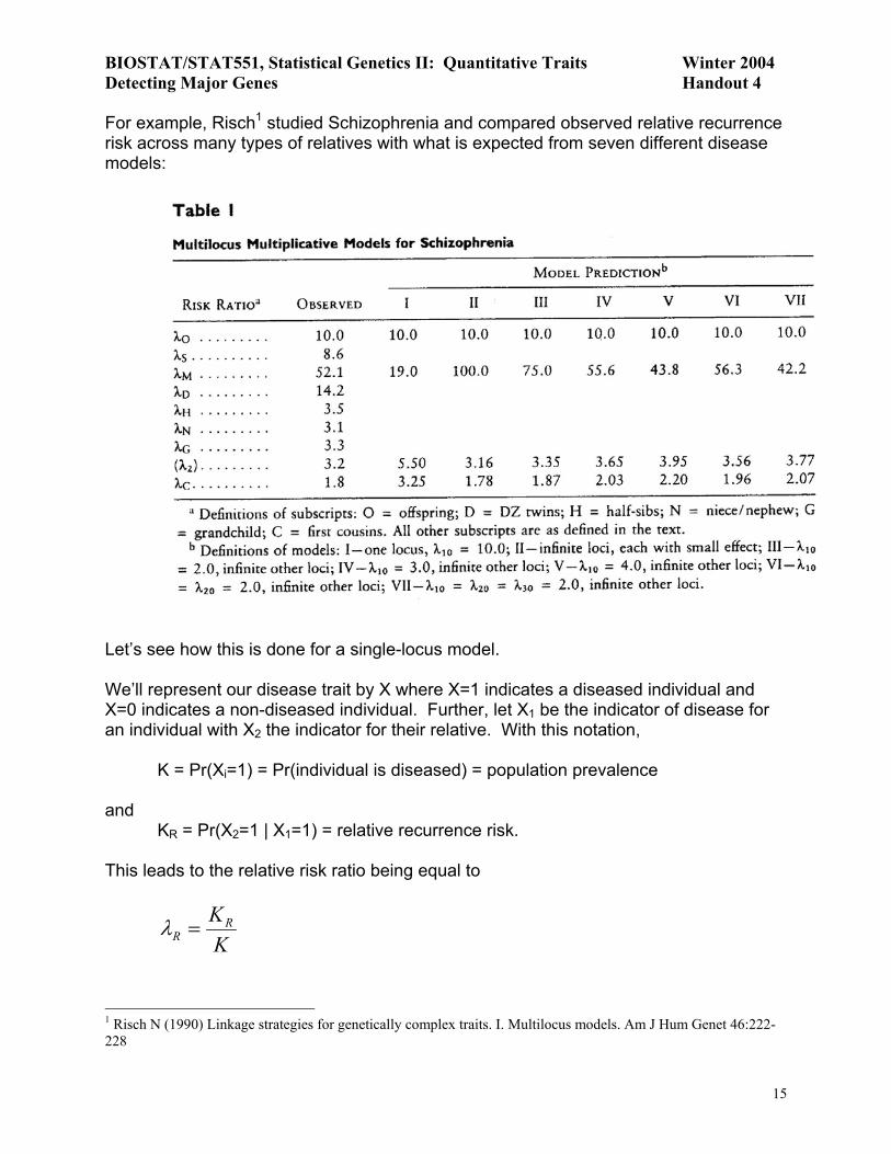
For example, Risch1 studied Schizophrenia and compared observed relative recurrence risk across many types of relatives with what is expected from seven different disease models:

Let’s see how this is done for a single-locus model. We’ll represent our disease trait by X where X=1 indicates a diseased individual and X=0 indicates a non-diseased individual. Further, let X1 be the indicator of disease for an individual with X2 the indicator for their relative. With this notation,

K = Pr(Xi=1) = Pr(individual is diseased) = population prevalence and

KR = Pr(X2=1 | X1=1) = relative recurrence risk.

This leads to the relative risk ratio being equal to

KKR

R =λ

1 Risch N (1990) Linkage strategies for genetically complex traits. I. Multilocus models. Am J Hum Genet 46:222-228


16

What is K equal to? For the single-locus model, assume there are two alleles, D and N, that are in Hardy-Weinberg Equilibrium with p=Pr(D).

=

×==

==

==

∑

∑

∈

∈

g) genotype has 1 ualPr(individg) genotype has 1 individual| 1Pr(

g) genotype has 1 individual and 1Pr( )1Pr(

}{1

}{1

1

genotypesg

genotypesg

X

XXK

Before we continue with the derivation of KR, let’s reconsider the biometrical model for the genotypic contribution to a trait. This will allow us to derive KR*K = Pr(X2=1, X1=1) = E(X1*X2) = Cov(X1,X2) + K2

Consider the phenotype Y where Y represents a standardized version of X as described below. Let fkl be the penetrance for genotype (k,l). We will treating the penetrance values as we previously used genotypic values. Let pk and pl represent allele frequencies for the kth and lth allele. We will also assume (for simplicity) that

0)( == ∑∑k l

lkkl ppfYE

Recall, the biometrical model breaks the genetic contribution into an effect due to each allele and the departure from these effects. We now apply this concept to the penetrances: lkklf αα += The αk and αl are chosen to minimize the deviations δkl = µkl - αk - αl using least squares. That is, they minimize ∑∑ −−=

k llklkkl ppfSS 2)( αα . From our previous work,

we then have:

∑=l

lklk pfα ,


17

and the variance in the genotypic contribution to the trait Y due to the additive effects of alleles or the additive genetic variance is

∑=k

kka p22 2 ασ

The variance due to departures from the additive effects of alleles or the dominance genetic variance is then

∑∑=k l

lkkld pp22 δσ

So that 2

722),cov( dijaijji YY σσ ∆+Φ= where ijΦ is the kinship coefficient and ij7∆ is the

coefficient of fraternity. We can now complete our derivation:

2

27

2

2

221

221

212

12

12

21

),(

)(

)1,1Pr(

/)1,1Pr(

)1|1Pr(

K

KKXXCov

KXXEKXXK

KXXKXX

KK

dijaij

RR

σσ

λ

∆+Φ+=

+=

=

===

===

===

=

(equation 4.1)

The last step was due to Y being a standardized version of X.


18

Example 4.5: Relatives of n degree are separated by n meioses. Parent-offspring pairs are first-degree relatives. Grandparent-grandchild and uncle-niece are second-degree relatives and first cousins are typical third-degree relatives. The following table summarizes the adjusted relative risk ratios for first, second and third-degree relatives.

R Relative Type Adjusted Risk Ratio (λR-1) 1 First-degree

2

2

2Kaσ

2 Second-degree 2

2

4Kaσ

3 Third-degree 2

2

8Kaσ

Summarize how the adjusted relative risk ratios for first, second and third degree relatives compare. How does this information help in study planning? Note that the above adjusted risk ratios are defined by equation 4.1 and the coefficients of kinship and fraternity. Below is a summary of these coefficients for reference. Table 2.1: Coefficients of kinship and fraternity for common relationships in a non-inbred population. Adapted from Lynch and Walsh2

Relationship ijΦ ij7∆ Parent-offspring 1/4 0 Grandparent-grandchild 1/8 0 Great grandparent-great grandchild 1/16 0 Half sibs 1/8 0 Full sibs, dizygotic twins 1/4 1/4 Uncle(aunt) – nephew(niece) 1/8 0 First cousins 1/16 0 Double first cousins 1/8 1/16 Second cousins 1/64 0 Monozygotic twins 1/2 1

2 Lynch M and Walsh B (1998) Genetics and analysis of quantitative traits. Sinauer Associates, Sunderland


19

Extension to multiple loci There are two general extensions that are used for relating susceptibility loci to disease risk: additive and multiplicative. • For an additive model, the Pr(disease given genotype i at locus 1 and genotype j at

locus 2) = Pr(disease given genotype 1 at locus 1) + Pr(disease given genotype 2 at locus 2). In this case,

)1()1(1 2

22

1

21 −

+−

=− RRR K

KKK λλλ where Ki is the prevalence of disease

due to locus i and λiR is the relative risk ratio for the ith locus

λ1-1 = 2(λ2-1)=4(λ3-1) where λi is the risk ratio for relatives of degree I (this is the same relationship as for a single locus)

we cannot distinguish a single locus from two (or multiple additive) loci

• For a multiplicative model, Pr(disease given genotype i at locus 1 and genotype j at

locus 2) = Pr(disease given genotype 1 at locus 1) × Pr(disease given genotype 2 at locus 2). In this case,

λR = λ1Rλ2R for relatives of type R

λ2 = λ12λ22 = 1/4(λ11+1) x (λ21+1) where λij is the relative recurrence risk for j

degree relatives for locus i

λ3 = 1/16 x (λ11+3) x (λ21+3)

note that the decay is greater than what is expected under the additive model


20

What does this provide us? Let’s answer this in the context of the example from Risch3. Consider the following in your discussion: − Based on the observed data, does an additive model fit the data well? − Note that λD > λS. What does this tell you? − Is there any evidence of dominance? The table on p18 might be useful here. − The risk to monozygotic twins is highly underestimated when fitting an additive

model. What does this imply? − What appears to be the most consistent model(s)?

3 Risch N (1990) Linkage strategies for genetically complex traits. I. Multilocus models. Am J Hum Genet 46:222-228

biostat/stat551, statistical genetics ii: quantitative...

Documents