birks n., meier g.h., pettit f.s. - introduction to the high-temperature oxidation of metals (2nd...
DESCRIPTION
High Temperature OxidationTRANSCRIPT


This page intentionally left blank
INTRODUCTION TO THE HIGH-TEMPERATUREOXIDATION OF METALS
A straightfoward treatment describing the oxidation processes of metals and alloysat elevated temperatures. This new edition retains the fundamental theory but incor-porates advances made in understanding degradation phenomena. Oxidation pro-cesses in complex systems are dicussed, from reactions in mixed environmentsto protective techniques, including coatings and atmosphere control. The authorsprovide a logical and expert treatment of the subject, producing a revised bookthat will be of use to students studying degradation of high-temperature materialsand an essential guide to researchers requiring an understanding of this elementaryprocess.
neil birks was Professor Emeritus in the Department of Materials Science andEngineering at the University of Pittsburgh.
gerald h. meier is William Kepler Whiteford Professor in the Department ofMaterials Science and Engineering at the University of Pittsburgh.
fred s. pettit is Harry S. Tack Professor in the Department of Materials Scienceand Engineering at the University of Pittsburgh.

INTRODUCTION TO THEHIGH-TEMPERATURE OXIDATION
OF METALS
2nd Edition
NEIL BIRKSFormerly of University of Pittsburgh
GERALD H. MEIERUniversity of Pittsburgh
FRED S. PETTITUniversity of Pittsburgh
cambridge university pressCambridge, New York, Melbourne, Madrid, Cape Town, Singapore, São Paulo
Cambridge University PressThe Edinburgh Building, Cambridge cb2 2ru, UK
First published in print format
isbn-13 978-0-521-48042-0
isbn-13 978-0-521-48517-3
isbn-13 978-0-511-16089-9
© N. Birks, G. H. Meier and F. S. Pettit 2006
2006
Information on this title: www.cambridge.org/9780521480420
This publication is in copyright. Subject to statutory exception and to the provision ofrelevant collective licensing agreements, no reproduction of any part may take placewithout the written permission of Cambridge University Press.
isbn-10 0-511-16089-5
isbn-10 0-521-48042-6
isbn-10 0-521-48517-7
Cambridge University Press has no responsibility for the persistence or accuracy of urlsfor external or third-party internet websites referred to in this publication, and does notguarantee that any content on such websites is, or will remain, accurate or appropriate.
Published in the United States of America by Cambridge University Press, New York
www.cambridge.org
hardback
eBook (EBL)
eBook (EBL)
hardback
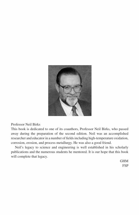
Professor Neil BirksThis book is dedicated to one of its coauthors, Professor Neil Birks, who passedaway during the preparation of the second edition. Neil was an accomplishedresearcher and educator in a number of fields including high-temperature oxidation,corrosion, erosion, and process metallurgy. He was also a good friend.
Neil’s legacy to science and engineering is well established in his scholarlypublications and the numerous students he mentored. It is our hope that this bookwill complete that legacy.
GHMFSP

Contents
Acknowledgements page viiiPreface ixIntroduction xi
1 Methods of investigation 12 Thermodynamic fundamentals 163 Mechanisms of oxidation 394 Oxidation of pure metals 755 Oxidation of alloys 1016 Oxidation in oxidants other than oxygen 1637 Reactions of metals in mixed environments 1768 Hot corrosion 2059 Erosion–corrosion of metals in oxidizing atmospheres 253
10 Protective coatings 27111 Atmosphere control for the protection of metals during production
processes 306Appendix A. Solution to Fick’s second law for a semi-infinite solid 323Appendix B. Rigorous derivation of the kinetics of internal oxidation 327Appendix C. Effects of impurities on oxide defect structures 332Index 336
vii
Acknowledgements
The authors gratefully acknowledge the scientific contributions of former and cur-rent students. Drs. J. M. Rakowski, M. J. Stiger, N. M. Yanar, and M. C. Maris-Sidaare thanked for their assistance in preparing figures for this book.
The authors also greatly appreciate the helpful comments made by Professor J. L.Beuth (Carnegie Mellon University), Professor H. J. Grabke (Max-Planck Institutfur Eisenforschung), and Professor R. A. Rapp (Ohio State University) on parts ofthe manuscript.
viii
Preface
Few metals, particularly those in common technological applications, are stablewhen exposed to the atmosphere at both high and low temperatures. Consequently,most metals in service today are subject to deterioration either by corrosion at roomtemperature or by oxidation at high temperature. The degree of corrosion varieswidely. Some metals, such as iron, will rust and oxidize very rapidly whereas othermetals, such as nickel and chromium, are attacked relatively slowly. It will be seenthat the nature of the surface layers produced on the metal plays a major role in thebehaviour of these materials in aggressive atmospheres.
The subject of high-temperature oxidation of metals is capable of extensiveinvestigation and theoretical treatment. It is normally found to be a very satisfyingsubject to study. The theoretical treatment covers a wide range of metallurgical,chemical, and physical principles and can be approached by people of a wide rangeof disciplines who, therefore, complement each other’s efforts.
Initially, the subject was studied with the broad aim of preventing the deterio-ration of metals in service, i.e., as a result of exposing the metal to high tempera-tures and oxidizing atmospheres. In recent years, a wealth of mechanistic data hasbecome available. These data cover a broad range of phenomena, e.g., mass transportthrough oxide scales, evaporation of oxide or metallic species, the role of mechan-ical stress in oxidation, growth of scales in complex environments containing morethan one oxidant, and the important relationships between alloy composition andmicrostructure and oxidation. Such information is obtained by applying virtuallyevery physical and chemical investigative technique to the subject.
In this book the intention is to introduce the subject of high-temperature oxi-dation of metals to students and to professional engineers whose work demandsfamiliarity with the subject. The emphasis of the book is placed firmly on supplyingan understanding of the basic, or fundamental, processes involved in oxidation.
In order to keep to this objective, there has been no attempt to provide an exhaus-tive, or even extensive, review of the literature. In our opinion this would increase
ix
Preface
the factual content without necessarily improving the understanding of the subjectand would, therefore, increase both the size and price of the book without enhanc-ing its objective as an introduction to the subject. Extensive literature quotation isalready available in books previously published on the subject and in review arti-cles. Similarly the treatment of techniques of investigation has been restricted to alevel that is sufficient for the reader to understand how the subject is studied with-out involving an overabundance of experimental details. Such details are availableelsewhere as indicated.
After dealing with the classical situations involving the straightforward oxida-tion of metals and alloys in the first five chapters, the final chapters extend thediscussion to reactions in mixed environments, i.e., containing more than one oxi-dant, to reactions involving a condensed phase as in hot corrosion, and the addedcomplications caused by erosive particles. Finally, some typical coatings for high-temperature applications and the use of protective atmospheres during processingare described.
Pittsburgh GHM2005 FSP
x
Introduction
The primary purpose of this book is to present an introduction to the fundamentalprinciples that govern the interaction of reactive gaseous environments (usuallycontaining oxygen as a component) and solid materials, usually metals, at hightemperatures. These principles are applicable to a variety of applications, whichcan include those where oxidation is desirable, such as forming a resistive silicalayer on silicon-based semiconductors or removing surface defects from steel slabsduring processing by rapid surface oxidation. However, most applications dealwith situations where reaction of the component with the gaseous atmosphere isundesirable and one tries to minimize the rate at which such reactions occur.
The term ‘high-temperature’ requires definition. In contrast to aqueous corrosion,the temperatures considered in this book will always be high enough that water,when present in the systems, will be present as the vapour rather than the liquid.Moreover, when exposed to oxidizing conditions at temperatures between 100and 500 ◦C, most metals and alloys form thin corrosion products that grow veryslowly and require transmission electron microscopy for detailed characterization.While some principles discussed in this book may be applicable to thin films, ‘hightemperature’ is considered to be 500 ◦C and above.
In designing alloys for use at elevated temperatures, the alloys must not only be asresistant as possible to the effects produced by reaction with oxygen, but resistanceto attack by other oxidants in the environment is also necessary. In addition, theenvironment is not always only a gas since, in practice, the deposition of ash on thealloys is not uncommon. It is, therefore, more realistic in these cases to speak ofthe high-temperature corrosion resistance of materials rather than their oxidationresistance.
The rate at which the reactions occur is governed by the nature of the reac-tion product which forms. In the case of materials such as carbon the reactionproduct is gaseous (CO and CO2), and does not provide a barrier to continuedreaction. The materials that are designed for high-temperature use are protected by
xi
Introduction
the formation of a solid reaction product (usually an oxide) which separates thecomponent and atmosphere. The rate of further reaction is controlled by transportof reactants through this solid layer. The materials designed for use at the high-est temperatures are ones which form the oxides with the slowest transport ratesfor reactants (usually α-Al2O3 or SiO2), i.e., those with the slowest growth rates.However, other materials are often used at lower temperatures if their oxides havegrowth rates which are ‘slow enough’ because they may have better mechanicalproperties (strength, creep resistance), may be easier to fabricate into components(good formability/weldability), or are less expensive.
In some cases, the barriers necessary to develop the desired resistance to corro-sion can be formed on structural alloys by appropriate composition modification.In many practical applications for structural alloys, however, the required compo-sitional changes are not compatible with the required physical properties of thealloys. In such cases, the necessary compositional modifications are developedthrough the use of coatings on the surfaces of the structural alloys and the desiredreaction-product barriers are developed on the surfaces of the coatings.
A rough hierarchy of common engineering alloys with respect to use temperaturewould include the following.
� Low-alloy steels, which form M3O4 (M = Fe, Cr) surface layers, are used to temperaturesof about 500 ◦C.
� Titanium-base alloys, which form TiO2, are used to about 600 ◦C.� Ferritic stainless steels, which form Cr2O3 surface layers, are used to about 650 ◦C. This
temperature limit is based on creep properties rather than oxidation rate.� Austenitic Fe–Ni–Cr alloys, which form Cr2O3 surface layers and have higher creep
strength than ferritic alloys, are used to about 850 ◦C.� Austenitic Ni–Cr alloys, which form Cr2O3 surface layers, are used to about 950 ◦C,
which is the upper limit for oxidation protection by chromia formation.� Austenitic Ni–Cr–Al alloys, and aluminide and MCrAlY (M = Ni, Co, or Fe) coatings,
which form Al2O3 surface layers, are used to about 1100 ◦C.� Applications above 1100 ◦C require the use of ceramics or refractory metals. The lat-
ter alloys oxidize catastrophically and must be coated with a more oxidation-resistantmaterial, which usually forms SiO2.
The exercise of ‘alloy selection’ for a given application takes all of the above factorsinto account. While other properties are mentioned from time to time, the emphasisof this book is on oxidation and corrosion behaviour.
xii
1
Methods of investigation
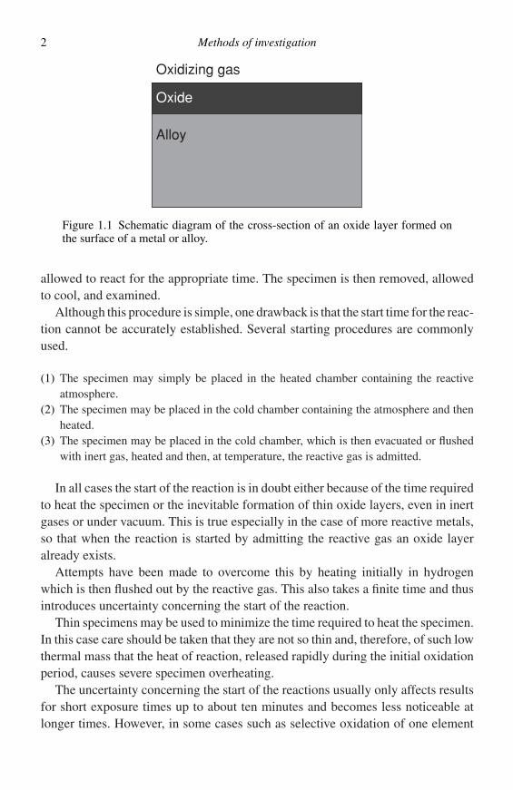
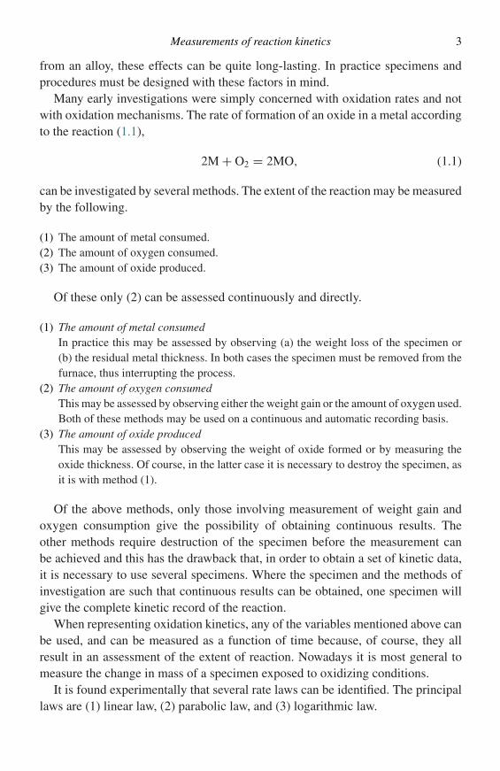
The investigation of high-temperature oxidation takes many forms. Usually oneis interested in the oxidation kinetics. Additionally, one is also interested in thenature of the oxidation process, i.e., the oxidation mechanism. Figure 1.1 is asimple schematic of the cross-section of an oxide formed on the surface of a metalor alloy. Mechanistic studies generally require careful examination of the reactionproducts formed with regard to their composition and morphology and often requireexamination of the metal or alloy substrate as well. Subsequent sections of thischapter will deal with the common techniques for measuring oxidation kineticsand examining reaction-product morphologies.
In measuring the kinetics of degradation and characterizing the correspond-ing microstructures questions arise as to the conditions to be used. Test condi-tions should be the same as the application under consideration. Unfortunately, theapplication conditions are often not precisely known and, even when known, canbe extremely difficult to establish as a controlled test. Moreover, true simulationtesting is usually impractical because the desired performance period is generallymuch longer than the length of time for which laboratory testing is feasible. Theanswer to this is accelerated, simulation testing.
Accelerated, simulation testing requires knowledge of microstructure and mor-phological changes. All materials used in engineering applications exhibit amicrostructural evolution, beginning during fabrication and ending upon termi-nation of their useful lives. In an accelerated test one must select test conditionsthat cause the microstructures to develop that are representative of the application,but in a much shorter time period. In order to use this approach some knowledgeof the degradation process is necessary.
Measurements of reaction kinetics
In the cases of laboratory studies, the experimental technique is basically simple.The specimen is placed in a furnace, controlled at the required temperature, and
1
2 Methods of investigation
Oxide
Oxidizing gas
Alloy
Figure 1.1 Schematic diagram of the cross-section of an oxide layer formed onthe surface of a metal or alloy.
allowed to react for the appropriate time. The specimen is then removed, allowedto cool, and examined.
Although this procedure is simple, one drawback is that the start time for the reac-tion cannot be accurately established. Several starting procedures are commonlyused.
(1) The specimen may simply be placed in the heated chamber containing the reactiveatmosphere.
(2) The specimen may be placed in the cold chamber containing the atmosphere and thenheated.
(3) The specimen may be placed in the cold chamber, which is then evacuated or flushedwith inert gas, heated and then, at temperature, the reactive gas is admitted.
In all cases the start of the reaction is in doubt either because of the time requiredto heat the specimen or the inevitable formation of thin oxide layers, even in inertgases or under vacuum. This is true especially in the case of more reactive metals,so that when the reaction is started by admitting the reactive gas an oxide layeralready exists.
Attempts have been made to overcome this by heating initially in hydrogenwhich is then flushed out by the reactive gas. This also takes a finite time and thusintroduces uncertainty concerning the start of the reaction.
Thin specimens may be used to minimize the time required to heat the specimen.In this case care should be taken that they are not so thin and, therefore, of such lowthermal mass that the heat of reaction, released rapidly during the initial oxidationperiod, causes severe specimen overheating.
The uncertainty concerning the start of the reactions usually only affects resultsfor short exposure times up to about ten minutes and becomes less noticeable atlonger times. However, in some cases such as selective oxidation of one element
Measurements of reaction kinetics 3
from an alloy, these effects can be quite long-lasting. In practice specimens andprocedures must be designed with these factors in mind.
Many early investigations were simply concerned with oxidation rates and notwith oxidation mechanisms. The rate of formation of an oxide in a metal accordingto the reaction (1.1),
2M + O2 = 2MO, (1.1)
can be investigated by several methods. The extent of the reaction may be measuredby the following.
(1) The amount of metal consumed.(2) The amount of oxygen consumed.(3) The amount of oxide produced.
Of these only (2) can be assessed continuously and directly.
(1) The amount of metal consumedIn practice this may be assessed by observing (a) the weight loss of the specimen or(b) the residual metal thickness. In both cases the specimen must be removed from thefurnace, thus interrupting the process.
(2) The amount of oxygen consumedThis may be assessed by observing either the weight gain or the amount of oxygen used.Both of these methods may be used on a continuous and automatic recording basis.
(3) The amount of oxide producedThis may be assessed by observing the weight of oxide formed or by measuring theoxide thickness. Of course, in the latter case it is necessary to destroy the specimen, asit is with method (1).
Of the above methods, only those involving measurement of weight gain andoxygen consumption give the possibility of obtaining continuous results. Theother methods require destruction of the specimen before the measurement canbe achieved and this has the drawback that, in order to obtain a set of kinetic data,it is necessary to use several specimens. Where the specimen and the methods ofinvestigation are such that continuous results can be obtained, one specimen willgive the complete kinetic record of the reaction.
When representing oxidation kinetics, any of the variables mentioned above canbe used, and can be measured as a function of time because, of course, they allresult in an assessment of the extent of reaction. Nowadays it is most general tomeasure the change in mass of a specimen exposed to oxidizing conditions.
It is found experimentally that several rate laws can be identified. The principallaws are (1) linear law, (2) parabolic law, and (3) logarithmic law.
4 Methods of investigation
(1) The linear law, for which the rate of reaction is independent of time, is found to referpredominantly to reactions whose rate is controlled by a surface-reaction step or bydiffusion through the gas phase.
(2) The parabolic law, for which the rate is inversely proportional to the square root oftime, is found to be obeyed when diffusion through the scale is the rate-determiningprocess.
(3) The logarithmic law is only observed for the formation of very thin films of oxide,i.e., between 2 and 4 nm, and is generally associated with low temperatures.
Under certain conditions some systems might even show composite kinetics,for instance niobium oxidizing in air at about 1000 ◦C initially conforms to theparabolic law but later becomes linear, i.e., the rate becomes constant at long times.
Discontinuous methods of assessment of reaction kinetics
In this case the specimen is weighed and measured and is then exposed to the con-ditions of high-temperature oxidation for a given time, removed, and reweighed.The oxide scale may also be stripped from the surface of the specimen, which isthen weighed. Assessment of the extent of reaction may be carried out quite sim-ply either by noting the mass gain of the oxidized specimen, which is the massof oxygen taken into the scale, or the mass loss of the stripped specimen, whichis equivalent to the amount of metal taken up in scale formation. Alternatively,the changes in specimen dimensions may be measured. As mentioned before thesetechniques yield only one point per specimen with the disadvantages that (a) manyspecimens are needed to plot fully the kinetics of the reaction, (b) the resultsfrom each specimen may not be equivalent because of experimental variations, and(c) the progress of the reaction between the points is not observed. On the other handthey have the obvious advantage that the techniques, and the apparatus required,are extremely simple. In addition, metallographic information is obtained for eachdata point.
Continuous methods of assessment
These methods fall into two types, those which monitor mass gain and those whichmonitor gas consumption.
Mass-gain methods
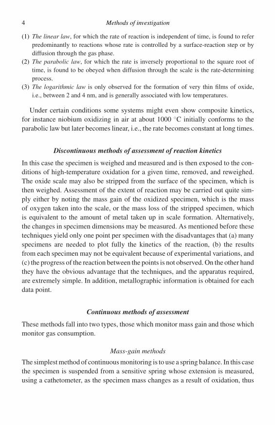
The simplest method of continuous monitoring is to use a spring balance. In this casethe specimen is suspended from a sensitive spring whose extension is measured,using a cathetometer, as the specimen mass changes as a result of oxidation, thus
Measurements of reaction kinetics 5
Gas exit tube(may be turned, raised, or lowered)
Serrated edge(allows point of suspension to be changed)
Pyrex tube
Cathetometer target
Silica or refractory tube with ground joint
Silica rod suspension
Specimen
Thermocouple
Gas inlet
Tube furnace
Pyrex or silicaspiral
Rigid epoxy resin joint
Figure 1.2 Features of a simple spring balance (for advanced design see ref. 1).
giving a semi-continuous monitoring of the reaction. Apparatus suitable for thisis shown diagrammatically in Figure 1.2 which is self-explanatory.1 An importantfeature is the design of the upper suspension point. In Figure 1.2 this is shownas a hollow glass tube which also acts as a gas outlet. The tube can be twisted,raised, or lowered to facilitate accurate placing of the specimen and alignment ofthe spring. A suspension piece is rigidly fastened to the glass tube and providesa serrated horizontal support for the spring whose suspension point may thus beadjusted in the horizontal plane. These refinements are required since alignmentbetween the glass tube containing the spring and the furnace tube is never perfectand it is prudent to provide some means of adjustment of the spring position in orderto ensure accurate placing of the specimen. It would be possible of course to equipa spring balance with a moving transformer, which would enable the mass gain to
6 Methods of investigation
be measured electrically, and automatically recorded. Although the simple springbalance should be regarded as a semi-continuous method of assessment, it has theadvantage that a complete reaction curve can be obtained from a single specimen.The disadvantage of the spring balance is that one is faced with a compromisebetween accuracy and sensitivity. For accuracy a large specimen is required whereasfor sensitivity one needs to use a relatively fragile spring. It is obviously not possibleto use a fragile spring to carry a large specimen and so the accuracy that is obtainedby this method is a matter of compromise between these two factors.
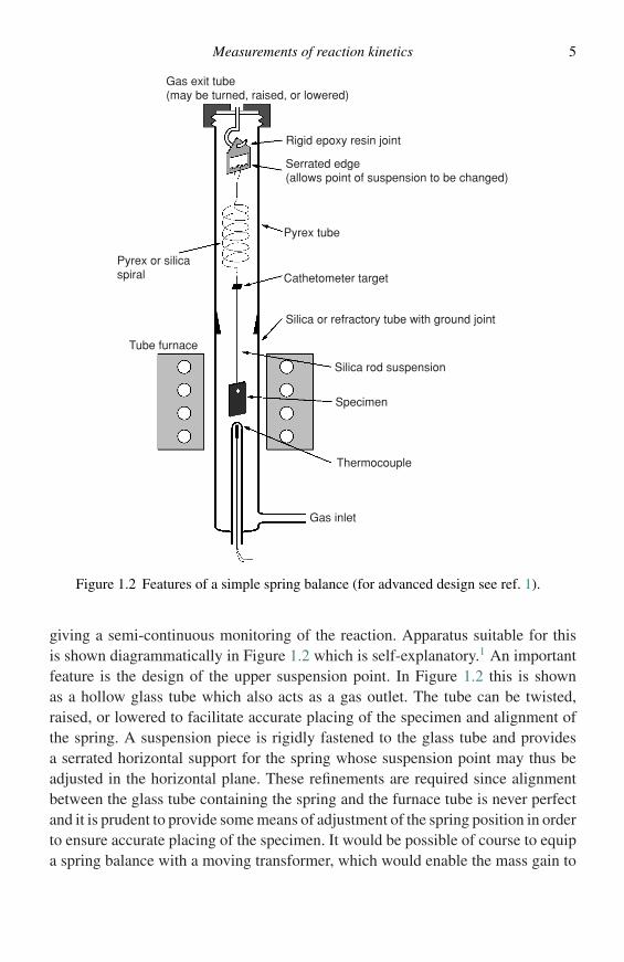
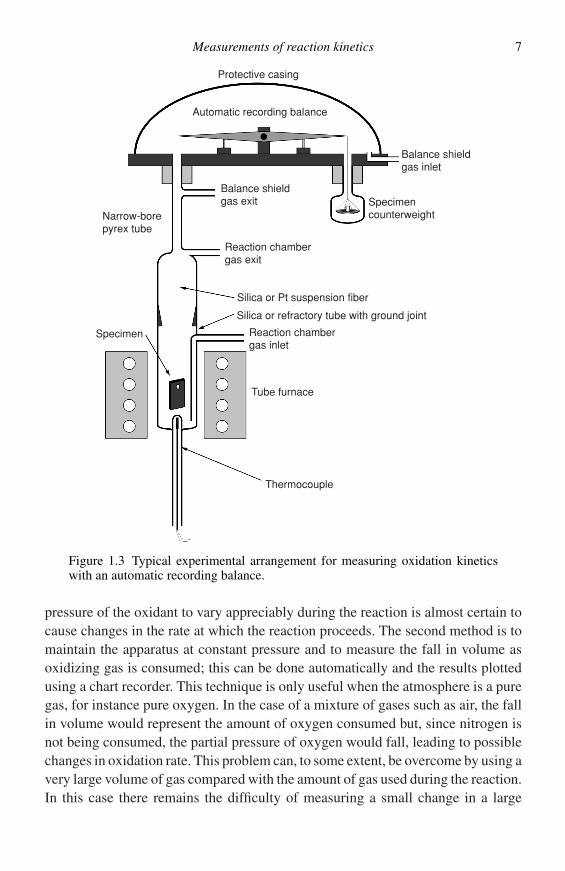
By far the most popular, most convenient, and, unfortunately, most expensivemethod of assessing oxidation reactions is to use the continuous automatic record-ing balance. Obviously the operator must decide precisely what is needed in termsof accuracy and sensitivity from the balance. For straightforward oxidation experi-ments it is generally adequate to choose a balance with a load-carrying ability of upto about 25 g and an ultimate sensitivity of about 100 µg. This is not a particularlysensitive balance and it is rather surprising that many investigators use far moresophisticated, and expensive, semi-micro balances for this sort of work. In factmany problems arise from the use of very sensitive balances together with smallspecimens, to achieve high accuracy. This technique is subject to errors causedby changes in Archimedean buoyancy when the gas composition is changed orthe temperature is altered. An error is also introduced as a result of a change indynamic buoyancy when the gas flow rate over the specimen is altered. For themost trouble-free operation it is advisable to use a large specimen with a large flatsurface area in conjunction with a balance of moderate accuracy. Figure 1.3 showsa schematic diagram of a continuously reading thermobalance used in the authors’laboratory.
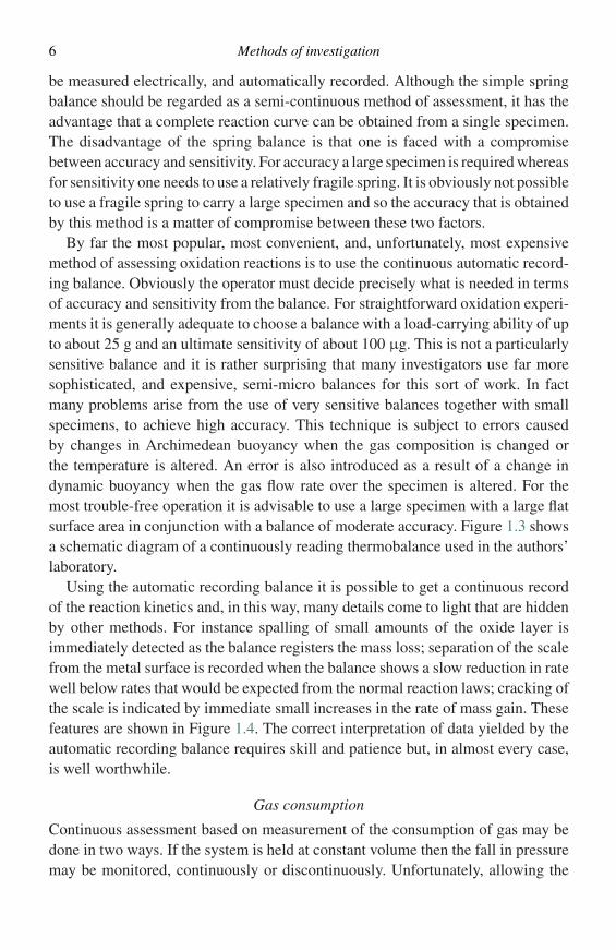
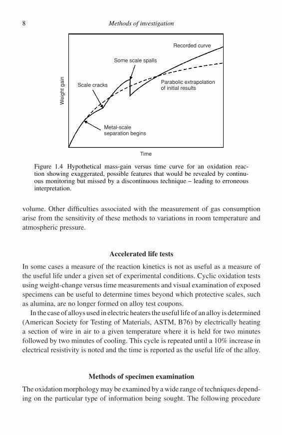
Using the automatic recording balance it is possible to get a continuous recordof the reaction kinetics and, in this way, many details come to light that are hiddenby other methods. For instance spalling of small amounts of the oxide layer isimmediately detected as the balance registers the mass loss; separation of the scalefrom the metal surface is recorded when the balance shows a slow reduction in ratewell below rates that would be expected from the normal reaction laws; cracking ofthe scale is indicated by immediate small increases in the rate of mass gain. Thesefeatures are shown in Figure 1.4. The correct interpretation of data yielded by theautomatic recording balance requires skill and patience but, in almost every case,is well worthwhile.
Gas consumption
Continuous assessment based on measurement of the consumption of gas may bedone in two ways. If the system is held at constant volume then the fall in pressuremay be monitored, continuously or discontinuously. Unfortunately, allowing the
Measurements of reaction kinetics 7
Protective casing
Automatic recording balance
Balance shieldgas exit
Reaction chambergas exit
Silica or Pt suspension fiber
Silica or refractory tube with ground joint
Reaction chambergas inlet
Tube furnace
Thermocouple
Specimen
Narrow-borepyrex tube
Specimencounterweight
Balance shieldgas inlet
Figure 1.3 Typical experimental arrangement for measuring oxidation kineticswith an automatic recording balance.
pressure of the oxidant to vary appreciably during the reaction is almost certain tocause changes in the rate at which the reaction proceeds. The second method is tomaintain the apparatus at constant pressure and to measure the fall in volume asoxidizing gas is consumed; this can be done automatically and the results plottedusing a chart recorder. This technique is only useful when the atmosphere is a puregas, for instance pure oxygen. In the case of a mixture of gases such as air, the fallin volume would represent the amount of oxygen consumed but, since nitrogen isnot being consumed, the partial pressure of oxygen would fall, leading to possiblechanges in oxidation rate. This problem can, to some extent, be overcome by using avery large volume of gas compared with the amount of gas used during the reaction.In this case there remains the difficulty of measuring a small change in a large
8 Methods of investigation
Recorded curve
Some scale spalls
Scale cracks
Metal-scaleseparation begins
Time
Wei
ght g
ain
Parabolic extrapolationof initial results
Figure 1.4 Hypothetical mass-gain versus time curve for an oxidation reac-tion showing exaggerated, possible features that would be revealed by continu-ous monitoring but missed by a discontinuous technique – leading to erroneousinterpretation.
volume. Other difficulties associated with the measurement of gas consumptionarise from the sensitivity of these methods to variations in room temperature andatmospheric pressure.
Accelerated life tests
In some cases a measure of the reaction kinetics is not as useful as a measure ofthe useful life under a given set of experimental conditions. Cyclic oxidation testsusing weight-change versus time measurements and visual examination of exposedspecimens can be useful to determine times beyond which protective scales, suchas alumina, are no longer formed on alloy test coupons.
In the case of alloys used in electric heaters the useful life of an alloy is determined(American Society for Testing of Materials, ASTM, B76) by electrically heatinga section of wire in air to a given temperature where it is held for two minutesfollowed by two minutes of cooling. This cycle is repeated until a 10% increase inelectrical resistivity is noted and the time is reported as the useful life of the alloy.
Methods of specimen examination
The oxidation morphology may be examined by a wide range of techniques depend-ing on the particular type of information being sought. The following procedure
Methods of specimen examination 9
is recommended in most instances. Initially, the specimen should be examined bythe naked eye and under a low-power binocular microscope, note being taken ofwhether the scale surface is flat, rippled, contains nodules, is cracked, or whetherthere is excessive attack on the edges or in the centers of the faces. This typeof examination is important because subsequent examination generally involvesmicroscopy of a section at a specific place and it is important to know whetherthis is typical or if there are variations over the specimen surface. It is often worth-while examining the surface in the scanning electron microscope, before sectioning,and, as with all examination, if an area is seen that has significant features, pho-tographs must be taken immediately. It is usually too late if one waits for a betteropportunity. In addition, modern scanning electron microscopes allow the chemicalcomposition of surface features to be determined. These techniques are describedbelow.
Having examined the scale, it is generally useful to perform X-ray diffraction(XRD) on it to obtain information on the phases present. Studies using XRD canalso provide auxiliary information such as the mechanical stress state in the scale,texture, etc.
Preparation of cross-section specimens
Once all the required information on the surface features has been obtained, it isgenerally useful to examine a cross-section of the specimen. This allows observationof the scale thickness and microstructure and any changes that have been producedin the underlying substrate.
Mounting
Metallographic examination involves polishing of a section and, under the polishingstresses, the scale is likely to fall away from the specimen. The specimen with itssurrounding scale must, therefore, be mounted. By far the best type of mountingmedium has been found to be the liquid epoxy resins. The process is very easy – adish is greased, the specimen is positioned and the resin is poured in. At this stagethe dish should be evacuated in a dessicator, left under vacuum for a few minutes,and then atmospheric pressure reapplied. This has the effect of removing air fromcrevices caused by cracks in the scale and on reapplying pressure the resin is forcedinto cavities left by evacuation. This sort of mounting procedure requires severalhours for hardening, preferably being left in a warm place overnight, but the goodsupport which is given to the fragile scales is well worth the extra time and effort.When emphasis must be placed on edge retention, it may be necessary to backupthe specimen with metal shims prior to the mounting operation.
10 Methods of investigation
Polishing
It is important at this stage to realize that polishing is carried out for the oxides andnot for the metal. A normal metallurgical polish will not reveal the full features ofthe oxide. Normally a metal is polished using successive grades of abrasive paper –the time spent on each paper being equivalent to the time required to remove thescratches left by the previous paper. If this procedure is carried out it will almostcertainly produce scales which are highly porous. It is important to realize that,because of their friability, scales are damaged to a greater depth than that repre-sented by the scratches on the metal, and, when going to a less abrasive paper, itis important to polish for correspondingly longer times in order to undercut thedepth of damage caused by the previous abrasive paper. In other words, polishingshould be carried out for much longer times on each paper than would be expectedfrom examination of the metal surface. If this procedure is carried out, scales whichare nicely compact and free from induced porosity will be revealed. The polishedspecimens may be examined using conventional optical metallography or scanningelectron microscopy (SEM).
Etching
Finally, it may be found necessary to etch a specimen to reveal detail in either themetal or the oxide scale. This is done following standard metallographic preparationprocedure with the exception that thorough and lengthy rinsing in a neutral solvent(alcohol) must be carried out. This is necessary because of existence of pores andcracks in the oxide, especially at the scale–metal interface, that retain the etchantby capillary action. Thus extensive soaking in rinse baths is advisable, followedby rapid drying under a hot air stream, if subsequent oozing and staining is to beavoided.
Description of specialized examination techniques
It is assumed that the reader is familiar with the techniques of optical microscopy.There are, however, a number of other specialized techniques, which are useful forexamining various features of oxidation morphologies. These techniques mainlygenerate information from interactions between the specimen and an incident beamof electrons, photons, or ions. The basis for the various techniques will be describedhere. Examples of their application will be presented in subsequent chapters.
Figure 1.5 is a schematic diagram of some of the important interactions between asolid specimen and an incident beam of electrons. The incident beam, if sufficientlyenergetic, can knock electrons from inner shells in the atoms in the solid givingrise to characteristic X-rays from each of the elements present as higher-energy
Description of specialized examination techniques 11
Incident electronbeam
Diffractedelectrons
Transmittedelectrons
Secondaryelectrons
Backscatteredelectrons
Auger electrons
Inelasticallyscattered electrons
CharacteristicX–rays
Figure 1.5 Schematic diagram of the interactions of an incident electron beamwith a solid specimen.
electrons fall into the empty states. Some of the electrons will be elastically scat-tered in the backward direction with the number of backscattered electrons, whichexit the specimen increasing as the average atomic mass of the solid increasesand as the local inclination of the specimen, with respect to the incident beam,increases. Secondary electrons are the result of inelastic scattering of electrons inthe conduction band of the solid, by incident or backscattered electrons, whichgives them enough energy to exit the solid. Auger electrons are ejected from thesolid by a process similar to that which generates characteristic X-rays, i.e., whena higher-energy electron falls into a vacated state, the energy released results inthe ejection of an electron from an outer shell rather than creation of an X-ray. Ifthe specimen is thin enough, some of the electrons will pass through the specimen.These will comprise a transmitted beam, which will contain electrons from theincident beam that have not undergone interactions or have lost energy as the resultof inelastic scattering processes, and a diffracted beam of electrons, which havesatisfied particular angular relations with lattice planes in the solid.
Figure 1.6 is a schematic diagram of some of the important interactions betweena solid specimen and an incident X-ray beam. These will result in diffractedX-rays, which have satisfied particular angular relations with lattice planes in thesolid and will, therefore, contain crystallographic information. The interactionswill also result in the ejection of photoelectrons, which will have energies equal tothe difference between that of the incident photon and the binding energy of theelectron in the state from which it is ejected.
12 Methods of investigation
Figure 1.6 Schematic diagram of the interactions of an incident X-ray beam witha solid specimen.
The following is a brief description of the electron-optical and other specializedtechniques, which may be used for examining oxidation morphologies, and thetype of information which may be obtained from each technique. The reader isdirected to the texts and reviews, referenced for each technique, for a more detaileddescription.
Scanning electron microscopy (SEM)
Scanning electron microscopy is currently the most widely used tool for charac-terising oxidation morphologies. In this technique2,3 an incident electron beam israstered over the specimen surface while the secondary electrons or backscatteredelectrons enter a detector creating an electrical signal which is used to modulatethe intensity of a TV monitor, which is being rastered at the same rate as theelectron beam. This produces an image which indicates the topography of the spec-imen, since the number of secondary or backscattered electrons which escape thespecimen will depend on the local tilt of the specimen surface, and does so withgreat depth of focus. Also, information regarding the average atomic mass can beobtained if the image is formed using backscattered electrons. Modern scanningelectron micrographs,3 equipped with field-emission electron guns, can achievemagnifications as high as 100 000 × and resolutions of 1000 nm.
Since the incident electrons also produce characteristic X-rays from the elementsin the solid, information can be obtained with regard to the elements present and,if suitable corrections are made, their concentration. The output from the X-ray
Description of specialized examination techniques 13
detector can also be used to modulate the intensity of the monitor, which allows amap of the relative concentration of a given element to be produced. The ability toprovide information with regard to microstructure and composition, simultaneously,makes SEM an extremely valuable tool in studying oxidation morphologies.
X-ray diffraction (XRD)
In this technique the specimen is bombarded with a focused beam of monochro-matic X-rays.4 The beam will be diffracted by the lattice planes, which satisfyBragg’s law, Equation (1.2), where λ is the wavelength of the X-rays, dhkl is
nλ = 2dhkl sin θ (1.2)
the interplanar spacing of the lattice plane, θ is the angle between the incident beamand the lattice plane, and n is the order of the reflection.
Determination of the angles at which diffraction occurs allows determinationof the spacing of the various lattice planes and, therefore, the crystal structure ofthe phase or phases present in the solid. Comparison of the d values with tab-ulated values for various substances can be used to identify the phases presentin the specimen. This has resulted in XRD being used for many years to iden-tify the phases present in oxide layers formed on metals and alloys. Modern X-raydiffractometers, with glancing-angle capabilities, can analyze oxide layers as thin as1000 nm.
An additional useful feature of XRD is that the positions of the diffraction peaksshift if the solid is strained. Use of specialized diffraction techniques5 allow thesestrains to be measured, which then allows determination of the state of stress in theoxide layer and, in some cases, the underlying metal substrate.
Transmission electron microscopy (TEM)
When higher spatial resolution examination of specimens is needed, transmissionelectron microscopy (TEM) is utilized.3,6 Here a specimen thin enough to transmitthe electron beam is required. This can be achieved by thinning the specimendirectly or mounting it and thinning a cross-section.7 If small precipitates are thefeature of interest, they can sometimes be examined by preparing carbon extractionreplicas from the specimen.
Figure 1.5 indicates that electrons, which have undergone several types of inter-action with the specimen, exit the bottom side. The transmitted beam has passedthrough the specimen with essentially no interaction. The diffracted beams con-tain electrons, which have not lost energy (elastically scattered) but have satisfiedangular criteria (similar to Bragg’s law for X-rays) and have been scattered intoa new path. The transmitted and diffracted beams can be used to form images ofthe specimen with very high resolution (on the order of 1 nm). Additionally the
14 Methods of investigation
diffracted electrons can be used to form a selected area diffraction (SAD) patternfrom a small region of the specimen, which yields crystallographic information ina manner analogous to XRD patterns.
Electrons which have lost energy by interaction with the specimen (inelasticallyscattered electrons) also exit the specimen. The amounts of energy lost by theelectrons can be measured and form the basis for several types of electron energy-loss spectroscopies (EELS) which allow high-resolution chemical analysis to beperformed.
Finally, characteristic X-rays are also produced in TEM, as they are in SEM,and can be analyzed to yield chemical-composition information. The X-rays aregenerated in a smaller specimen volume in TEM than SEM and, therefore, smallerfeatures can be analyzed.
Surface analytical techniques
In many cases it is of interest to have information about compositions in very thinlayers of materials, such as the first-formed oxide on an alloy. A group of techniques,which are highly surface sensitive, are available for such determinations.8 Grabkeet al.9 have presented a good review of the application of these techniques in theanalysis of oxidation problems.
The most widely used technique is Auger electron spectroscopy (AES). Sincethe Auger electrons are emitted as the result of transitions between electron levels,their energies are element specific and all elements, with the exception of H andHe, can be detected.9 Also, since the energies of Auger electrons are low (20eV–2.5 keV) they are only emitted from shallow depths, of a few atomic layers,giving the technique its surface sensitivity. Auger spectra can be quantified usingstandards and published correction factors, and if the incident beam is scanned overthe specimen surface, can be used to generate composition maps analogous to theX-ray maps from a scanning electron micrograph. The incident electron beam inmodern instruments can be focussed to give analyses with lateral spatial resolutionon the order of 50 nm.9
The photoelectrons produced by bombarding the specimens with X-rays can alsobe used to obtain chemical information in a technique called X-ray photoelectronspectroscopy (XPS). Photoelectrons have energies similar to Auger electrons sothe specimen depth analyzed is similar to that in AES. However, since it is difficultto bring an X-ray beam to a fine focus the spatial resolution is poorer than thatachievable in AES. An advantage of XPS is that, since the photoelectron energy isa function of the binding energy of the electron in the solid, it can give informationregarding the ionization state of an element, i.e., whether it is present in elementalform, as an oxide, as a nitride, etc.
References 15
Secondary-ion mass spectroscopy (SIMS) is another useful technique, whichinvolves sputtering away the surface of the specimen with an ion beam and analyzingthe sputtered ions in a mass spectrometer. The SIMS technique can provide veryprecise chemical analysis of very thin surface layers and, as sputtering proceeds, aconcentration–depth profile through the specimen.
The application of the above techniques is an important part of the study ofoxidation, so much so that regular conferences are now held on this subject.10–14
It is important to emphasize that proper investigation of oxidation mechanismsinvolves as many of the above techniques of observing kinetics and morphologiesas feasible, and careful combination of the results.
References
1. S. Mrowec and A. J. Stoklosa, J. Therm. Anal., 2 (1970), 73.2. J. I. Goldstein, D. E. Newbury, P. Echlin, et al., Scanning Electron Microscopy and
X-Ray Microanalysis, New York, NY, Plenum Press, 1984.3. M. H. Loretto, Electron Beam Analysis of Materials, 2nd edn., London, UK,
Chapman and Hall, 1994.4. B. D. Cullity, Elements of X-Ray Diffraction, 2nd edn, Reading, MA, Addison
Wesley, 1978.5. I. C. Noyan and J. B. Cohen, Residual Stresses, New York, NY, Springer-Verlag,
1987.6. D. B. Williams and C. B. Carter, Transmission Electron Microscopy, New York, NY,
Plenum Press, 1996.7. M. Ruhle, U. Salzberger and E. Schumann. High resolution transmission microscopy
of metal/metal oxide interfaces. In Microscopy of Oxidation 2, eds. S. B. Newcomband M. J. Bennett, London, UK, The Institute of Materials, 1993, p. 3.
8. D. P. Woodruff and T. A. Delchar, Modern Techniques of Surface Science,Cambridge, UK, Cambridge University Press, 1989.
9. H. J. Grabke, V. Leroy and H. Viefhaus, ISIJ Int., 35 (1995), 95.10. Microscopy of Oxidation 1, eds. M. J. Bennett and G. W. Lorimer, London, UK, The
Institute of Metals, 1991.11. Microscopy of Oxidation 2, eds. S. B. Newcomb and M. J. Bennett, London, UK,
The Institute of Materials, 1993.12. Microscopy of Oxidation 3, eds. S. B. Newcomb and J. A. Little, London, UK, The
Institute of Materials, 1997.13. Microscopy of Oxidation 4, eds. G. Tatlock and S. B. Newcomb, Science Rev., 17
(2000), 1.14. Microscopy of Oxidation 5, eds. G. Tatlock and S. B. Newcomb, Science Rev., 20
(2003).
2
Thermodynamic fundamentals
Introduction
A sound understanding of high-temperature corrosion reactions requires the deter-mination of whether or not a given component in a metal or alloy can react with agiven component from the gas phase or another condensed phase, and to rationalizeobserved products of the reactions. In practice, the corrosion problems to be solvedare often complex, involving the reaction of multicomponent alloys with gases con-taining two or more reactive components. The situation is often complicated by thepresence of liquid or solid deposits, which form either by condensation from thevapour or impaction of particulate matter. An important tool in the analysis of suchproblems is, of course, equilibrium thermodynamics which, although not predic-tive, allows one to ascertain which reaction products are possible, whether or notsignificant evaporation or condensation of a given species is possible, the conditionsunder which a given reaction product can react with a condensed deposit, etc. Thecomplexity of the corrosion phenomena usually dictates that the thermodynamicanalysis be represented in graphical form.
The purpose of this chapter is to review the thermodynamic concepts pertinentto gas–metal reactions and then to describe the construction of the thermodynamicdiagrams most often used in corrosion research, and to present illustrative examplesof their application. The types of diagrams discussed are
(1) Gibbs free energy versus composition diagrams and activity versus composition dia-grams, which are used for describing the thermodynamics of solutions.
(2) Standard free energy of formation versus temperature diagrams which allow the ther-modynamic data for a given class of compounds, oxides, sulphides, carbides, etc., tobe presented in a compact form.
(3) Vapour-species diagrams which allow the vapour pressures of compounds to bepresented as a function of convenient variables such as partial pressure of a gaseouscomponent.
16
Basic thermodynamics 17
(4) Two-dimensional, isothermal stability diagrams, which map the stable phases in systemsinvolving one metallic and two reactive, non-metallic components.
(5) Two-dimensional, isothermal stability diagrams which map the stable phases in systemsinvolving two metallic components and one reactive, non-metallic component.
(6) Three-dimensional, isothermal stability diagrams which map the stable phases in sys-tems involving two metallic and two reactive, non-metallic components.
Basic thermodynamics
The question of whether or not a reaction can occur is answered by the second law ofthermodynamics. Since the conditions most often encountered in high-temperaturereactions are constant temperature and pressure, the second law is most convenientlywritten in terms of the Gibbs free energy (G′) of a system, Equation (2.1),
G ′ = H ′ − T S′, (2.1)
where H′ is the enthalpy and S′ the entropy of the system. Under these conditionsthe second law states that the free-energy change of a process will have the follow-ing significance: �G ′ < 0, spontaneous reaction expected; �G ′ = 0, equilibrium;�G ′ > 0, thermodynamically impossible process.
For a chemical reaction, e.g. Equation (2.2),
aA + bB = cC + dD, (2.2)
�G′ is expressed as in Equation (2.3),
�G ′ = �G◦ + RT ln
(ac
CadD
aaAab
B
), (2.3)
where �G◦ is the free-energy change when all species are present in their standardstates; a is the thermodynamic activity, which describes the deviation from thestandard state for a given species and may be expressed for a given species i as inEquation (2.4),
ai = pi
p◦i
. (2.4)
Here pi is either the vapour pressure over a condensed species or the partial pressureof a gaseous species and p◦
i is the same quantity corresponding to the standard stateof i. Expressing ai by Equation (2.4) requires the reasonable approximation ofideal gas behaviour at the high temperatures and relatively low pressures usuallyencountered. The standard free-energy change is expressed for a reaction such asEquation (2.2) by Equation (2.5),
�G◦ = c�G◦C + d�G◦
D − a�G◦A − b�G◦
B, (2.5)
18 Thermodynamic fundamentals
where �G◦C, etc., are standard molar free energies of formation which may be
obtained from tabulated values. (A selected list of references for thermodynamicdata such as �G◦ is included at the end of this chapter.) For the special cases ofequilibrium (�G ′ = 0) Equation (2.3) reduces to Equation (2.6),
�G◦ = −RT ln
(ac
CadD
aaAab
B
)eq
. (2.6)
The term in parentheses is called the equilibrium constant (K) and is used to describethe equilibrium state of the reaction system.
Construction and use of thermodynamic diagrams
(a) Gibbs free energy versus composition diagrams and activity versuscomposition diagrams
The equilibrium state of a system at constant temperature and pressure is charac-terized by a minimum in the Gibbs free energy of the system. For a multicom-ponent, multiphase system, the minimum free energy corresponds to uniformityof the chemical potential (µ) of each component throughout the system. For abinary system, the molar free energy (G) and chemical potentials are related byEquation (2.7),
G = (1 − X )µA + XµB, (2.7)
where µA and µB are the chemical potentials of components A and B, respectively,and (l − X) and X are the mole fractions of A and B. Figure 2.1(a) is a plot of Gversus composition for a single phase which exhibits simple solution behaviour. Itcan readily be shown,1,2 starting with Equation (2.7), that for a given compositionµA and µB can be defined as in Equations (2.8) and (2.9),
µA = G − XdG
dX; (2.8)
µB = G + (1 − X )dG
dX, (2.9)
which, as indicated in Figure 2.1(a), means that a tangent drawn to the free-energycurve has intercepts on the ordinate at X = 0 and X = 1, corresponding to thechemical potentials of A and B, respectively. Alternatively, if the free energy ofthe unmixed components in their standard states, (1 − X )µ◦
A + Xµ◦B is subtracted
from each side of Equation (2.7), the result is the molar free energy of mixing,Equation (2.10):
�GM = (1 − X )(µA − µ◦A) + X (µB − µ◦
B). (2.10)
Construction and use of thermodynamic diagrams 19
G
µBG α
G β
µB
A BX ←
X ←
µA
G
←
µA
G
←
(a)
(1−X ) –––dGdX
βα α+β
A BX1 X2
(b)
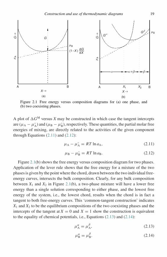
Figure 2.1 Free energy versus composition diagrams for (a) one phase, and(b) two coexisting phases.
A plot of �GM versus X may be constructed in which case the tangent interceptsare (µA − µ◦
A) and (µB − µ◦B), respectively. These quantities, the partial molar free
energies of mixing, are directly related to the activities of the given componentthrough Equations (2.11) and (2.12):
µA − µ◦A = RT ln aA, (2.11)
µB − µ◦B = RT ln aB. (2.12)
Figure 2.1(b) shows the free energy versus composition diagram for two phases.Application of the lever rule shows that the free energy for a mixture of the twophases is given by the point where the chord, drawn between the two individual free-energy curves, intersects the bulk composition. Clearly, for any bulk compositionbetween X1 and X2 in Figure 2.1(b), a two-phase mixture will have a lower freeenergy than a single solution corresponding to either phase, and the lowest freeenergy of the system, i.e., the lowest chord, results when the chord is in fact atangent to both free-energy curves. This ‘common-tangent construction’ indicatesX1 and X2 to be the equilibrium compositions of the two coexisting phases and theintercepts of the tangent at X = 0 and X = 1 show the construction is equivalentto the equality of chemical potentials, i.e., Equations (2.13) and (2.14):
µαA = µ
β
A, (2.13)
µαB = µ
β
B. (2.14)
20 Thermodynamic fundamentals
� �
a�
a�
�
a
←
←X�
←X �
a�
a�
���a
←
�
� ����
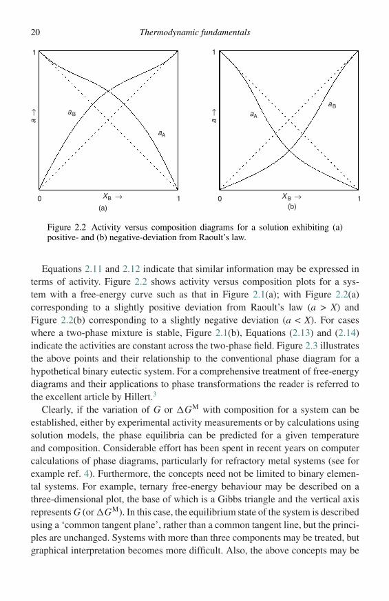
Figure 2.2 Activity versus composition diagrams for a solution exhibiting (a)positive- and (b) negative-deviation from Raoult’s law.
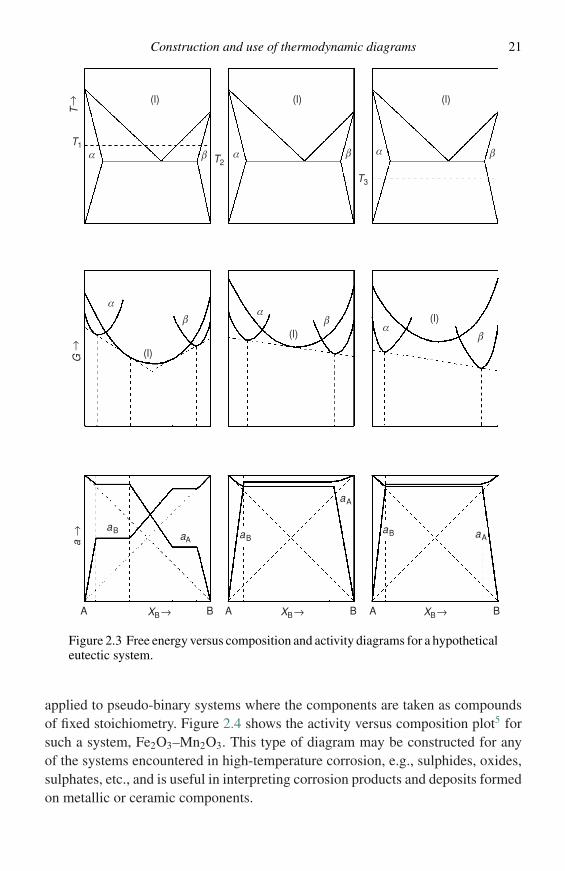
Equations 2.11 and 2.12 indicate that similar information may be expressed interms of activity. Figure 2.2 shows activity versus composition plots for a sys-tem with a free-energy curve such as that in Figure 2.1(a); with Figure 2.2(a)corresponding to a slightly positive deviation from Raoult’s law (a > X) andFigure 2.2(b) corresponding to a slightly negative deviation (a < X). For caseswhere a two-phase mixture is stable, Figure 2.1(b), Equations (2.13) and (2.14)indicate the activities are constant across the two-phase field. Figure 2.3 illustratesthe above points and their relationship to the conventional phase diagram for ahypothetical binary eutectic system. For a comprehensive treatment of free-energydiagrams and their applications to phase transformations the reader is referred tothe excellent article by Hillert.3
Clearly, if the variation of G or �GM with composition for a system can beestablished, either by experimental activity measurements or by calculations usingsolution models, the phase equilibria can be predicted for a given temperatureand composition. Considerable effort has been spent in recent years on computercalculations of phase diagrams, particularly for refractory metal systems (see forexample ref. 4). Furthermore, the concepts need not be limited to binary elemen-tal systems. For example, ternary free-energy behaviour may be described on athree-dimensional plot, the base of which is a Gibbs triangle and the vertical axisrepresents G (or �GM). In this case, the equilibrium state of the system is describedusing a ‘common tangent plane’, rather than a common tangent line, but the princi-ples are unchanged. Systems with more than three components may be treated, butgraphical interpretation becomes more difficult. Also, the above concepts may be
Construction and use of thermodynamic diagrams 21
G
←
a
←
T
←
T1
T2
T3
α β α β α β
(l) (l)
αβ
(l)α
β(l)
α
β
(l)
(l)
aB aBaA
aA
aB aA
BABABA XB
← XB
← XB
←
Figure 2.3 Free energy versus composition and activity diagrams for a hypotheticaleutectic system.
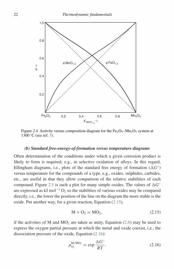
applied to pseudo-binary systems where the components are taken as compoundsof fixed stoichiometry. Figure 2.4 shows the activity versus composition plot5 forsuch a system, Fe2O3–Mn2O3. This type of diagram may be constructed for anyof the systems encountered in high-temperature corrosion, e.g., sulphides, oxides,sulphates, etc., and is useful in interpreting corrosion products and deposits formedon metallic or ceramic components.
22 Thermodynamic fundamentals
Mn2O3Fe2O3
a FeO1.5a MnO1.5
X MnO1.5→
a →
0.2 0.4 0.6 0.8
0.8
0.6
0.4
0.2
1.0
Figure 2.4 Activity versus composition diagram for the Fe2O3–Mn2O3 system at1300 ◦C (see ref. 5).
(b) Standard free-energy-of-formation versus temperature diagrams
Often determination of the conditions under which a given corrosion product islikely to form is required, e.g., in selective oxidation of alloys. In this regard,Ellingham diagrams, i.e., plots of the standard free energy of formation (�G◦)versus temperature for the compounds of a type, e.g., oxides, sulphides, carbides,etc., are useful in that they allow comparison of the relative stabilities of eachcompound. Figure 2.5 is such a plot for many simple oxides. The values of �G◦
are expressed as kJ mol−1 O2 so the stabilities of various oxides may be compareddirectly, i.e., the lower the position of the line on the diagram the more stable is theoxide. Put another way, for a given reaction, Equation (2.15),
M + O2 = MO2, (2.15)
if the activities of M and MO2 are taken as unity, Equation (2.6) may be used toexpress the oxygen partial pressure at which the metal and oxide coexist, i.e., thedissociation pressure of the oxide, Equation (2.16):
pM/MO2O2
= exp�G◦
RT. (2.16)
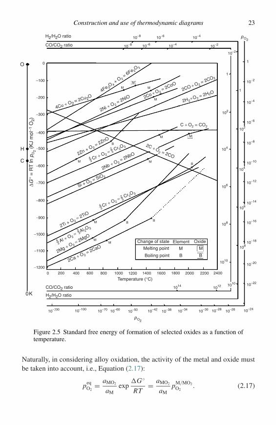
Construction and use of thermodynamic diagrams 23
H2/H2O ratio
CO/CO2 ratio
H2/H2O ratio
CO/CO2 ratio
10−8
10−2410−2610−2810−3010−3410−3810−4210−5010−6010−7010−10010−200
10−8
10−6
10−6
10−4
10−2
10−2
102
102
104
104
106
106
108
108
1010
101010121014
10−4
10−8
10−10
10−12
10−14
10−16
10−18
10−20
10−22
10−6
10−4
10−2
1
1
1
0K
0 200 400 600 800 1000 1200 1400 1600 1800 2000 2200 2400
pO2
pO2
Temperature (°C)
Change of state Element Oxide
Melting point
Boiling point
M M
B B
0
−100
−200
−300
−400
−500
−600
−700
−800
−900
−1000
−1100
−1200
O
H
C
∆G°
= R
T ln
pO
2 (K
J m
ol−1
O2)
4Cu + O2= 2Cu2O4Fe 3
O 4 + O 2
= 6Fe 2O 3
M
M
M
M
M
MM
M
MM
M
B
B
BB
2Ni + O 2 = 2NiO 2Co + O2
= 2CoO2CO + O2 =
2CO2
2H2+O2 = 2H2O
C + O2 = CO2
2C + O2 = 2CO2Zn + O 2
= 2ZnO
43
23
Cr + O2 = C
r2O3
43
23
Cr + O2 = C
r2O3
43
23
Al + O 2 = A
l 2O 3
2Nb + O 2 = 2NbO
Si + O2 = SiO2
2Ti + O 2 = 2TiO
2Mg + O 2 = 2MgO
2Ca + O2 = 2CaO
Figure 2.5 Standard free energy of formation of selected oxides as a function oftemperature.
Naturally, in considering alloy oxidation, the activity of the metal and oxide mustbe taken into account, i.e., Equation (2.17):
peqO2
= aMO2
aMexp
�G◦
RT= aMO2
aMpM/MO2
O2. (2.17)
24 Thermodynamic fundamentals
The values of pM/MO2O2
may be obtained directly from the oxygen nomograph onthe diagram by drawing a straight line from the origin marked O through the free-energy line at the temperature of interest and reading the oxygen partial pressurefrom its intersection with the scale at the right side labelled pO2. Values for thepressure ratio H2/H2O for equilibrium between a given metal and oxide may beobtained by drawing a similar line from the point marked H to the scale labelledH2/H2O ratio and values for the equilibrium CO/CO2 ratio may be obtained bydrawing a line from point C to the scale CO/CO2 ratio. The reader is referred toGaskell (ref. 2, Chapter 12), for a more detailed discussion of the construction anduse of Ellingham diagrams for oxides.
Ellingham diagrams may, of course, be constructed for any class of compounds.Shatynski has published Ellingham diagrams for sulphides6 and carbides.7 Elling-ham diagrams for nitrides and chlorides are presented in chapter 14 of reference 1.
(c) Vapour-species diagrams
The vapour species which form in a given high-temperature corrosion situation oftenhave a strong influence on the rate of attack, the rate generally being acceleratedwhen volatile corrosion products form. Gulbransen and Jansson8 have shown thatmetal and volatile oxide species are important in the kinetics of high-temperatureoxidation of carbon, silicon, molybdenum, and chromium. Six types of oxidationphenomena were identified.
(1) At low temperature, diffusion of oxygen and metal species through a compact oxidefilm.
(2) At moderate and high temperatures, a combination of oxide-film formation and oxidevolatility.
(3) At moderate and high temperatures, the formation of volatile metal and oxide speciesat the metal–oxide interface and transport through the oxide lattice and mechanicallyformed cracks in the oxide layer.
(4) At moderate and high temperatures, the direct formation of volatile oxide gases.(5) At high temperature, the gaseous diffusion of oxygen through a barrier layer of
volatilised oxides.(6) At high temperature, spalling of metal and oxide particles.
Sulphidation reactions follow a similar series of kinetic phenomena as has beenobserved for oxidation. Unfortunately, few studies have been made of the basickinetic phenomena involved in sulphidation reactions at high temperature. Simi-larly, the volatile species in sulphate and carbonate systems are important in termsof evaporation/condensation phenomena involving these compounds on alloy orceramic surfaces. Perhaps the best example of this behaviour is the rapid degra-dation of protective scales on many alloys, termed ‘hot corrosion’, which occurswhen Na2SO4 or other salt condenses on the alloy.
Construction and use of thermodynamic diagrams 25
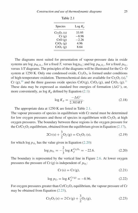
Table 2.1
Species Log Kp
Cr2O3 (s) 33.95Cr (g) −8.96
CrO (g) −2.26CrO2 (g) 4.96CrO3 (g) 8.64
The diagrams most suited for presentation of vapour-pressure data in oxidesystems are log pMx Oy , for a fixed T, versus logpO2; and log pMx Oy , for a fixed pO2,versus 1/T diagrams. The principles of the diagrams will be illustrated for the Cr–Osystem at 1250 K. Only one condensed oxide, Cr2O3, is formed under conditionsof high-temperature oxidation. Thermochemical data are available for Cr2O3 (s),9
Cr (g),10 and the three gaseous oxide species CrO (g), CrO2 (g), and CrO3 (g).11
These data may be expressed as standard free energies of formation (�G◦), or,more conveniently, as log Kp defined by Equation (2.1):
log K p = −�G◦
2.303RT. (2.18)
The appropriate data at 1250 K are listed in Table 2.1.The vapour pressures of species in equilibrium with Cr metal must be determinedfor low oxygen pressures and those of species in equilibrium with Cr2O3 at highoxygen pressures. The boundary between these regions is the oxygen pressure forthe Cr/Cr2O3 equilibrium, obtained from the equilibrium given in Equation (2.17),
2Cr (s) + 3
2O2 (g) = Cr2O3 (s), (2.19)
for which log pO2 has the value given in Equation (2.20):
log pO2 = −2
3log K Cr2O3
p = −22.6. (2.20)
The boundary is represented by the vertical line in Figure 2.6. At lower oxygenpressures the pressure of Cr (g) is independent of pO2:
Cr (s) = Cr (g), (2.21)
log pCr = log K Cr (g)p = −8.96. (2.22)
For oxygen pressures greater than Cr/Cr2O3 equilibrium, the vapour pressure of Crmay be obtained from Equation (2.23),
Cr2O3 (s) = 2 Cr (g) + 3
2O2 (g), (2.23)
26 Thermodynamic fundamentals
log (p −H2/p−H2O)
log
p C
r xO
y (a
tm)
Cr(s)
Cr(g)
CrO(g)
CrO 2 (g)
CrO 3 (g)
Cr2O3 (s)
14 12 10 8 6 4 2 0 −2
−4
−8
−12
−16
−20
−24
−44 −40 −36 −32 −28 −24 −20 −16 −12 −8 −4 0
−4 −64
0
log p O2(atm)
Figure 2.6 Volatile species in the Cr–O system at 1250 K.
with the equilibrium constant, K23, determined from Equation (2.24):
log K23 = 2 log K Cr (g)p − log K Cr2O3
p = −51.9. (2.24)
Therefore, Equations (2.25) or (2.26) are obtained:
2 log pCr + 3
2log pO2 = −51.9, (2.25)
log pCr = −25.95 − 3
4log pO2 . (2.26)
The vapour pressure of Cr is then expressed in Figure 2.6 by plotting Equations(2.22) and (2.26). The lines corresponding to the other vapour species are obtainedin the same manner. For example, for CrO3 at oxygen pressures below Cr/Cr2O3
equilibrium we have Equations (2.27) and (2.28):
Cr (s) + 3
2O2 (g) = CrO3 (g), (2.27)
log K27 = log K CrO3 (g)p = 8.64, (2.28)
from which one finds log pCrO3 , Equation (2.29):
log pCrO3 = 8.64 + 3
2log pO2 . (2.29)
Construction and use of thermodynamic diagrams 27
T (K)
log
p Cr x
Oy (a
tm)
1/T × 103 (K−1)
Cr(g)
Cr2O3(s)/O2
Cr2O3(s)/Cr(s)
CrO3(g)
Mixedoxidationand volatility
Enhancedoxidationdue to Crvapour
Normaloxidation
1150 1200 1250 1300 1342 1400 1450
0
−2
−4
−6
−8
−10
−12
−140.88 0.86 0.84 0.82 0.80 0.78 0.76 0.74 0.72 0.70 0.68
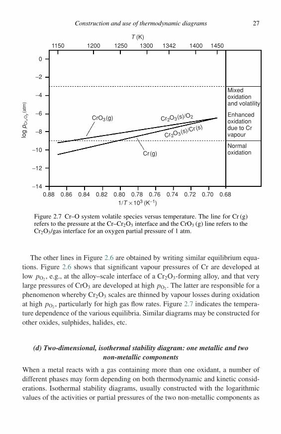
Figure 2.7 Cr–O system volatile species versus temperature. The line for Cr (g)refers to the pressure at the Cr–Cr2O3 interface and the CrO3 (g) line refers to theCr2O3/gas interface for an oxygen partial pressure of 1 atm.
The other lines in Figure 2.6 are obtained by writing similar equilibrium equa-tions. Figure 2.6 shows that significant vapour pressures of Cr are developed atlow pO2, e.g., at the alloy–scale interface of a Cr2O3-forming alloy, and that verylarge pressures of CrO3 are developed at high pO2. The latter are responsible for aphenomenon whereby Cr2O3 scales are thinned by vapour losses during oxidationat high pO2, particularly for high gas flow rates. Figure 2.7 indicates the tempera-ture dependence of the various equilibria. Similar diagrams may be constructed forother oxides, sulphides, halides, etc.
(d) Two-dimensional, isothermal stability diagram: one metallic and twonon-metallic components
When a metal reacts with a gas containing more than one oxidant, a number ofdifferent phases may form depending on both thermodynamic and kinetic consid-erations. Isothermal stability diagrams, usually constructed with the logarithmicvalues of the activities or partial pressures of the two non-metallic components as
28 Thermodynamic fundamentals
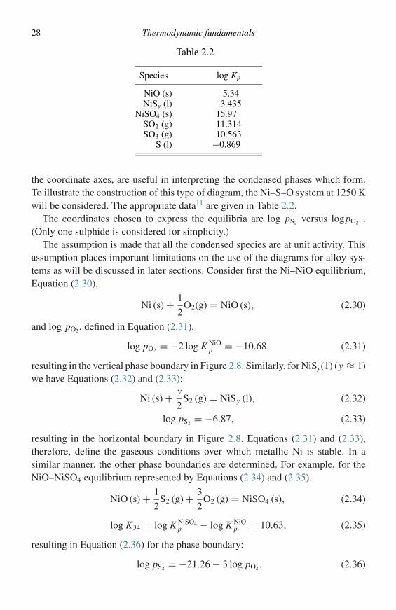
Table 2.2
Species log Kp
NiO (s) 5.34NiSy (l) 3.435
NiSO4 (s) 15.97SO2 (g) 11.314SO3 (g) 10.563
S (l) −0.869
the coordinate axes, are useful in interpreting the condensed phases which form.To illustrate the construction of this type of diagram, the Ni–S–O system at 1250 Kwill be considered. The appropriate data11 are given in Table 2.2.
The coordinates chosen to express the equilibria are log pS2 versus logpO2 .(Only one sulphide is considered for simplicity.)
The assumption is made that all the condensed species are at unit activity. Thisassumption places important limitations on the use of the diagrams for alloy sys-tems as will be discussed in later sections. Consider first the Ni–NiO equilibrium,Equation (2.30),
Ni (s) + 1
2O2(g) = NiO (s), (2.30)
and log pO2, defined in Equation (2.31),
log pO2 = −2 log K NiOp = −10.68, (2.31)
resulting in the vertical phase boundary in Figure 2.8. Similarly, for NiSy(1) (y ≈ 1)we have Equations (2.32) and (2.33):
Ni (s) + y
2S2 (g) = NiSy (l), (2.32)
log pS2 = −6.87, (2.33)
resulting in the horizontal boundary in Figure 2.8. Equations (2.31) and (2.33),therefore, define the gaseous conditions over which metallic Ni is stable. In asimilar manner, the other phase boundaries are determined. For example, for theNiO–NiSO4 equilibrium represented by Equations (2.34) and (2.35).
NiO (s) + 1
2S2 (g) + 3
2O2 (g) = NiSO4 (s), (2.34)
log K34 = log K NiSO4p − log K NiO
p = 10.63, (2.35)
resulting in Equation (2.36) for the phase boundary:
log pS2 = −21.26 − 3 log pO2 . (2.36)
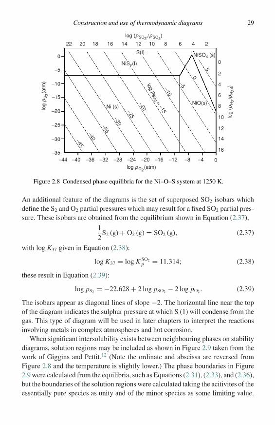
Construction and use of thermodynamic diagrams 29
Ni (s)NiO(s)
NiSO4 (s)
NiSy(I)
log pso
2 = −15
log
(pH
2/p
H2S
)
log (pSO2 /pSO3)
log
pS
2(a
tm)
log pO2(atm)
S(I)
16
14
12
10
8
6
4
22 20 18 16 14 12 10 8 6 4 2
2
00
−5
−5−10
−20
−10
−25−30−35−40−45
−15
−20
−25
−30
−350−44 −40 −36 −32 −28 −24 −20 −16 −12 −8 −4
5
0
Figure 2.8 Condensed phase equilibria for the Ni–O–S system at 1250 K.
An additional feature of the diagrams is the set of superposed SO2 isobars whichdefine the S2 and O2 partial pressures which may result for a fixed SO2 partial pres-sure. These isobars are obtained from the equilibrium shown in Equation (2.37),
1
2S2 (g) + O2 (g) = SO2 (g), (2.37)
with log K37 given in Equation (2.38):
log K37 = log K SO2p = 11.314; (2.38)
these result in Equation (2.39):
log pS2 = −22.628 + 2 log pSO2 − 2 log pO2 . (2.39)
The isobars appear as diagonal lines of slope −2. The horizontal line near the topof the diagram indicates the sulphur pressure at which S (1) will condense from thegas. This type of diagram will be used in later chapters to interpret the reactionsinvolving metals in complex atmospheres and hot corrosion.
When significant intersolubility exists between neighbouring phases on stabilitydiagrams, solution regions may be included as shown in Figure 2.9 taken from thework of Giggins and Pettit.12 (Note the ordinate and abscissa are reversed fromFigure 2.8 and the temperature is slightly lower.) The phase boundaries in Figure2.9 were calculated from the equilibria, such as Equations (2.31), (2.33), and (2.36),but the boundaries of the solution regions were calculated taking the acitivites of theessentially pure species as unity and of the minor species as some limiting value.
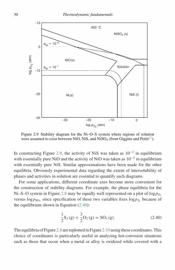
30 Thermodynamic fundamentals
900 °C
NiSO4 (s)
−10
−10
−20
−30 −10−20−30 0
0
NiO(s)
Ni(s) NiS (I)
log
pO
2 (at
m)
log pS2 (atm)
Solution
aNi = 10−6
aNi = 10−1
Figure 2.9 Stability diagram for the Ni–O–S system where regions of solutionwere assumed to exist between NiO, NiS, and NiSO4 (from Giggins and Pettit12).
In constructing Figure 2.9, the activity of NiS was taken as 10−2 in equilibriumwith essentially pure NiO and the activity of NiO was taken as 10−2 in equilibriumwith essentially pure NiS. Similar approximations have been made for the otherequilibria. Obviously experimental data regarding the extent of intersolubility ofphases and activities in solution are essential to quantify such diagrams.
For some applications, different coordinate axes become more convenient forthe construction of stability diagrams. For example, the phase equilibria for theNi–S–O system in Figure 2.8 may be equally well represented on a plot of logpO2
versus logpSO3 since specification of these two variables fixes logpS2 because ofthe equilibrium shown in Equation (2.40):
1
2S2 (g) + 3
2O2 (g) = SO3 (g). (2.40)
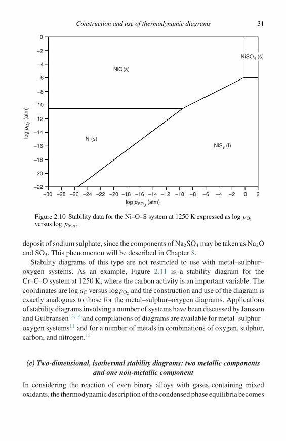
The equilibria of Figure 2.8 are replotted in Figure 2.10 using these coordinates. Thischoice of coordinates is particularly useful in analyzing hot-corrosion situationssuch as those that occur when a metal or alloy is oxidized while covered with a
Construction and use of thermodynamic diagrams 31
NiO(s)
NiSO4 (s)
NiSy (I)Ni(s)
log pSO3 (atm)
log
pO
2 (at
m)
0
−2
−4
−6
−8
−10
−12
−14
−16
−18
−20
−18 −16 −14 −12 −10 −8 −6 −4 −2 0 2−20−30 −28 −26 −24 −22−22
Figure 2.10 Stability data for the Ni–O–S system at 1250 K expressed as log pO2
versus log pSO3 .
deposit of sodium sulphate, since the components of Na2SO4 may be taken as Na2Oand SO3. This phenomenon will be described in Chapter 8.
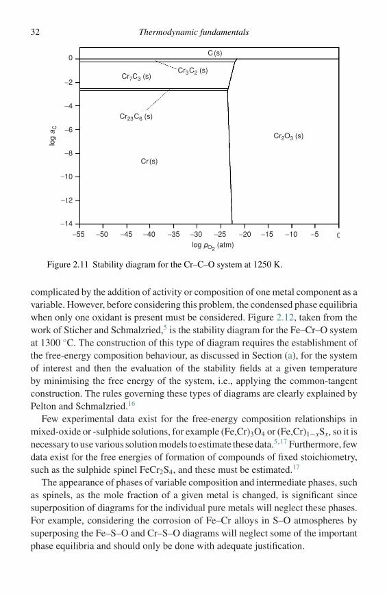
Stability diagrams of this type are not restricted to use with metal–sulphur–oxygen systems. As an example, Figure 2.11 is a stability diagram for theCr–C–O system at 1250 K, where the carbon activity is an important variable. Thecoordinates are log aC versus logpO2 and the construction and use of the diagram isexactly analogous to those for the metal–sulphur–oxygen diagrams. Applicationsof stability diagrams involving a number of systems have been discussed by Janssonand Gulbransen13,14 and compilations of diagrams are available for metal–sulphur–oxygen systems11 and for a number of metals in combinations of oxygen, sulphur,carbon, and nitrogen.15
(e) Two-dimensional, isothermal stability diagrams: two metallic componentsand one non-metallic component
In considering the reaction of even binary alloys with gases containing mixedoxidants, the thermodynamic description of the condensed phase equilibria becomes
32 Thermodynamic fundamentals
C(s)
Cr(s)
Cr7C3 (s)
Cr23C6 (s)
Cr3C2 (s)
Cr2O3 (s)
log
aC
0
−2
−4
−6
−8
−10
−12
−14
−55 −50 −45 −40 −35 −30 −25 −20 −15 −10 −5 0log pO2
(atm)
Figure 2.11 Stability diagram for the Cr–C–O system at 1250 K.
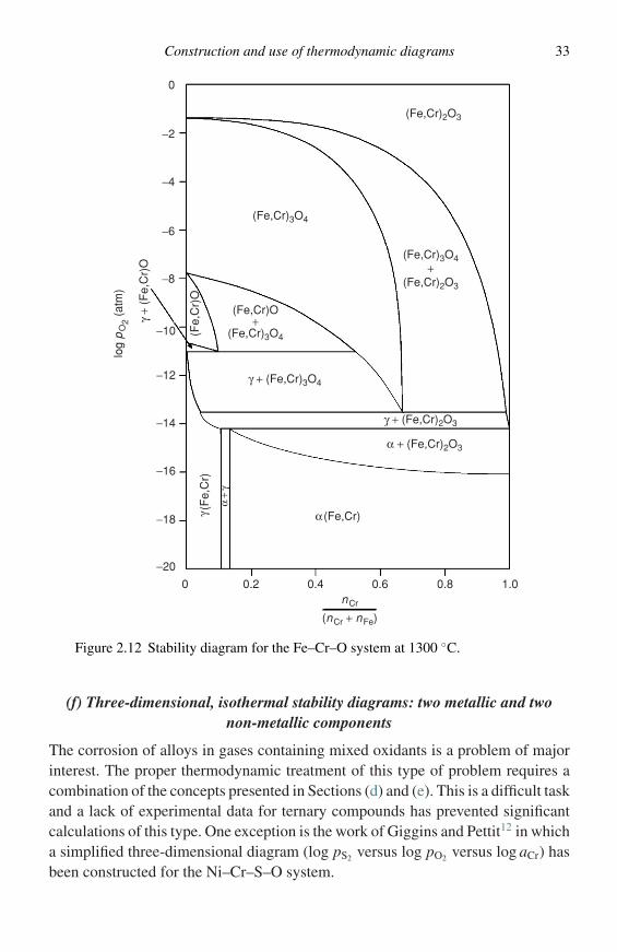
complicated by the addition of activity or composition of one metal component as avariable. However, before considering this problem, the condensed phase equilibriawhen only one oxidant is present must be considered. Figure 2.12, taken from thework of Sticher and Schmalzried,5 is the stability diagram for the Fe–Cr–O systemat 1300 ◦C. The construction of this type of diagram requires the establishment ofthe free-energy composition behaviour, as discussed in Section (a), for the systemof interest and then the evaluation of the stability fields at a given temperatureby minimising the free energy of the system, i.e., applying the common-tangentconstruction. The rules governing these types of diagrams are clearly explained byPelton and Schmalzried.16
Few experimental data exist for the free-energy composition relationships inmixed-oxide or -sulphide solutions, for example (Fe,Cr)3O4 or (Fe,Cr)1−xSx, so it isnecessary to use various solution models to estimate these data.5,17 Furthermore, fewdata exist for the free energies of formation of compounds of fixed stoichiometry,such as the sulphide spinel FeCr2S4, and these must be estimated.17
The appearance of phases of variable composition and intermediate phases, suchas spinels, as the mole fraction of a given metal is changed, is significant sincesuperposition of diagrams for the individual pure metals will neglect these phases.For example, considering the corrosion of Fe–Cr alloys in S–O atmospheres bysuperposing the Fe–S–O and Cr–S–O diagrams will neglect some of the importantphase equilibria and should only be done with adequate justification.
Construction and use of thermodynamic diagrams 33
0
−2
−4
−6
−8
−10
−12
−14
−16
−18
−20
0 0.2 0.4 0.6 0.8 1.0
(Fe,Cr)2O3
(Fe,Cr)3O4
(Fe,Cr)3O4+
(Fe,Cr)2O3
(Fe,Cr)O+
(Fe,Cr)3O4
log
pO
2 (at
m)
γ +
(Fe,
Cr)
O
γ + (Fe,Cr)3O4
γ + (Fe,Cr)2O3
α + (Fe,Cr)2O3
α (Fe,Cr)γ (F
e,C
r)
α+
γ
(Fe,
Cr)
O
nCr
(nCr + nFe)
Figure 2.12 Stability diagram for the Fe–Cr–O system at 1300 ◦C.
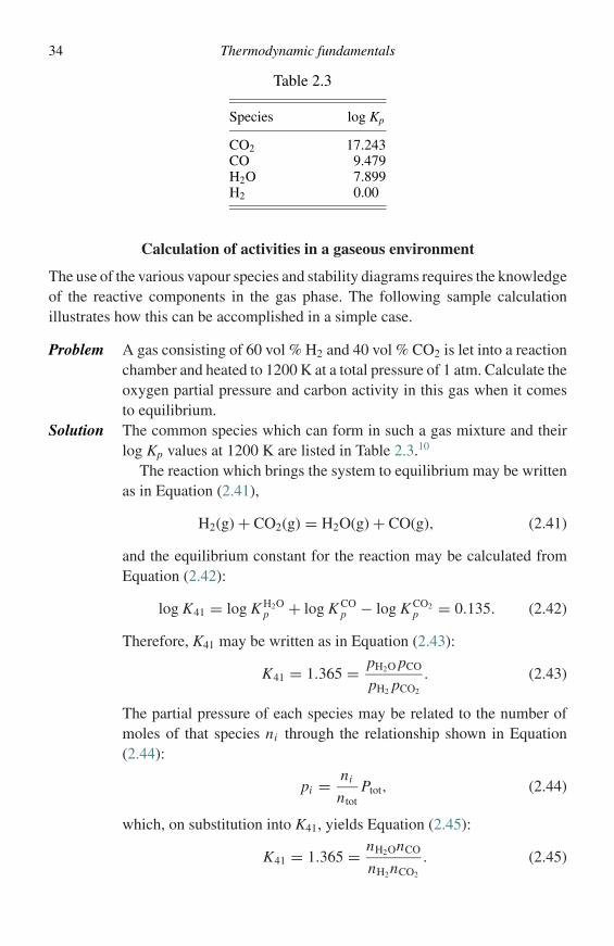
(f) Three-dimensional, isothermal stability diagrams: two metallic and twonon-metallic components
The corrosion of alloys in gases containing mixed oxidants is a problem of majorinterest. The proper thermodynamic treatment of this type of problem requires acombination of the concepts presented in Sections (d) and (e). This is a difficult taskand a lack of experimental data for ternary compounds has prevented significantcalculations of this type. One exception is the work of Giggins and Pettit12 in whicha simplified three-dimensional diagram (log pS2 versus log pO2 versus log aCr) hasbeen constructed for the Ni–Cr–S–O system.
34 Thermodynamic fundamentals
Table 2.3
Species log Kp
CO2 17.243CO 9.479H2O 7.899H2 0.00
Calculation of activities in a gaseous environment
The use of the various vapour species and stability diagrams requires the knowledgeof the reactive components in the gas phase. The following sample calculationillustrates how this can be accomplished in a simple case.
Problem A gas consisting of 60 vol % H2 and 40 vol % CO2 is let into a reactionchamber and heated to 1200 K at a total pressure of 1 atm. Calculate theoxygen partial pressure and carbon activity in this gas when it comesto equilibrium.
Solution The common species which can form in such a gas mixture and theirlog Kp values at 1200 K are listed in Table 2.3.10
The reaction which brings the system to equilibrium may be writtenas in Equation (2.41),
H2(g) + CO2(g) = H2O(g) + CO(g), (2.41)
and the equilibrium constant for the reaction may be calculated fromEquation (2.42):
log K41 = log K H2Op + log K CO
p − log K CO2p = 0.135. (2.42)
Therefore, K41 may be written as in Equation (2.43):
K41 = 1.365 = pH2O pCO
pH2 pCO2
. (2.43)
The partial pressure of each species may be related to the number ofmoles of that species ni through the relationship shown in Equation(2.44):
pi = ni
ntotPtot, (2.44)
which, on substitution into K41, yields Equation (2.45):
K41 = 1.365 = nH2OnCO
nH2nCO2
. (2.45)
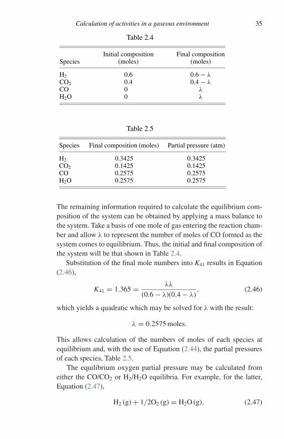
Calculation of activities in a gaseous environment 35
Table 2.4
Initial composition Final compositionSpecies (moles) (moles)
H2 0.6 0.6 − λCO2 0.4 0.4 − λCO 0 λH2O 0 λ
Table 2.5
Species Final composition (moles) Partial pressure (atm)
H2 0.3425 0.3425CO2 0.1425 0.1425CO 0.2575 0.2575H2O 0.2575 0.2575
The remaining information required to calculate the equilibrium com-position of the system can be obtained by applying a mass balance tothe system. Take a basis of one mole of gas entering the reaction cham-ber and allow λ to represent the number of moles of CO formed as thesystem comes to equilibrium. Thus, the initial and final composition ofthe system will be that shown in Table 2.4.
Substitution of the final mole numbers into K41 results in Equation(2.46),
K41 = 1.365 = λλ
(0.6 − λ)(0.4 − λ), (2.46)
which yields a quadratic which may be solved for λ with the result:
λ = 0.2575 moles.
This allows calculation of the numbers of moles of each species atequilibrium and, with the use of Equation (2.44), the partial pressuresof each species, Table 2.5.
The equilibrium oxygen partial pressure may be calculated fromeither the CO/CO2 or H2/H2O equilibria. For example, for the latter,Equation (2.47),
H2 (g) + 1/2O2 (g) = H2O (g), (2.47)
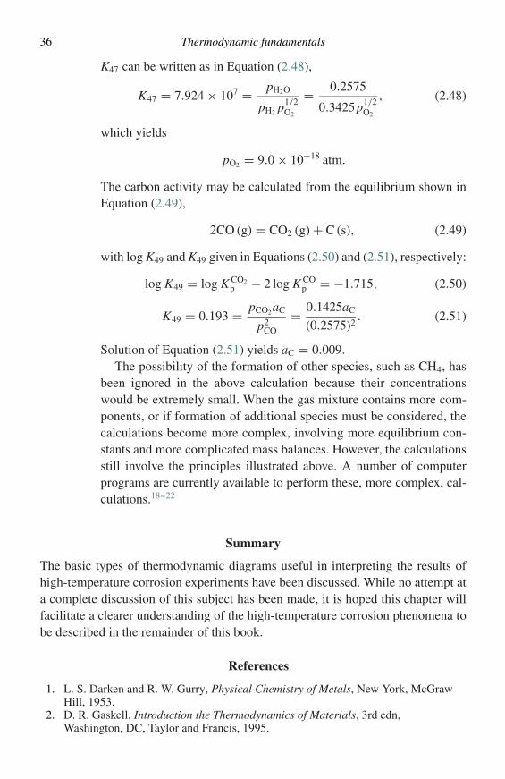
36 Thermodynamic fundamentals
K47 can be written as in Equation (2.48),
K47 = 7.924 × 107 = pH2O
pH2 p1/2O2
= 0.2575
0.3425p1/2O2
, (2.48)
which yields
pO2 = 9.0 × 10⁻¹⁸ atm.
The carbon activity may be calculated from the equilibrium shown inEquation (2.49),
2CO (g) = CO2 (g) + C (s), (2.49)
with log K49 and K49 given in Equations (2.50) and (2.51), respectively:
log K49 = log K CO2p − 2 log K CO
p = −1.715, (2.50)
K49 = 0.193 = pCO2aC
p2CO
= 0.1425aC
(0.2575)2. (2.51)
Solution of Equation (2.51) yields aC = 0.009.
The possibility of the formation of other species, such as CH4, hasbeen ignored in the above calculation because their concentrationswould be extremely small. When the gas mixture contains more com-ponents, or if formation of additional species must be considered, thecalculations become more complex, involving more equilibrium con-stants and more complicated mass balances. However, the calculationsstill involve the principles illustrated above. A number of computerprograms are currently available to perform these, more complex, cal-culations.18–22
Summary
The basic types of thermodynamic diagrams useful in interpreting the results ofhigh-temperature corrosion experiments have been discussed. While no attempt ata complete discussion of this subject has been made, it is hoped this chapter willfacilitate a clearer understanding of the high-temperature corrosion phenomena tobe described in the remainder of this book.
References
1. L. S. Darken and R. W. Gurry, Physical Chemistry of Metals, New York, McGraw-Hill, 1953.
2. D. R. Gaskell, Introduction the Thermodynamics of Materials, 3rd edn,Washington, DC, Taylor and Francis, 1995.
References 37
3. M. Hillert, The uses of Gibbs free energy–composition diagrams. In Lectures on theTheory of Phase Transformations, 2nd edn, ed. H. I. Aaronson, Warrendale, PA, TheMinerals, Metals and Materials Society, 1999.
4. L. Kaufman and H. Bernstein, Computer calculations of refractory metal phasediagrams. In Phase Diagrams, Materials Science and Technology, ed. A. M. Alper,New York, Academic Press, 1970, vol. 1.
5. J. Sticher and H. Schmalzried, Zur geometrischen Darstellung thermodynamischerZustandsgrossen in Mehrstoffsystemen auf Eisenbasis. Report, Clausthal Institute furTheoretische Huttenkunde und Angewandte Physikalische Chemie der TechnischenUniversitat Clausthal, 1975.
6. S. R. Shatynski, Oxid. Met., 11 (1977), 307.7. S. R. Shatynski, Oxid, Met., 13 (1979), 105.8. E. A. Gulbransen and S. A. Jansson, In Heterogeneous Kinetics at Elevated
Temperatures, eds. G. R. Belton and W. R. Worrell, New York, Plenum Press, 1970,p. 181.
9. C. E. Wicks and F. E. Block, Thermodynamic properties of 65 elements, their oxides,halides, carbides, and nitrides. Bureau of Mines, Bulletin 605, Washington, DC, USGovernment Printing Office, 1963, p. 408.
10. JANAF Thermochemical Tables, J. Phys. Chemi. Ref. Data, 4 (1975), 1–175.11. E. A. Gulbransen and G. H. Meier, Themodynamic stability diagrams for condensed
phases and volatility diagrams for volatile species over condensed phases in twentymetal–sulfur–oxygen systems between 1150 and 1450 K. University of Pittsburgh,DOE Report on Contract no. DE-AC01–79-ET-13547, May, 1979.
12. C. S. Giggins and F. S. Pettit, Oxid. Met., 14 (1980), 363.13. G. H. Meier, N. Birks, F. S. Pettit, and C. S. Giggins, Thermodynamic analyses of
high temperature corrosion of alloys in gases containing more than one reactant. InHigh Temperature Corrosion, ed. R. A. Rapp, Houston, TX, NACE, 1983, p. 327.
14. S. A. Jansson and E. A. Gulbransen, Thermochemical considerations of hightemperature gas-solid reactions. In High Temperature Gas–Metal Reactions in MixedEnvironments, ed. S. A. Jansson and Z. A. Foroulis, New York, American Institute ofMining, Metallurgical, and Petroleum Engineerings, 1973, p. 2.
15. P. L. Hemmings and R. A. Perkins, Thermodynamic phase stability diagrams for theanalysis of corrosion reactions in coal gasification/combusion atmospheres. ResearchProject 716–1, Interim Report, Palo Alto, CA, Lockheed Palo Alto ResearchLaboratories for Electric Power Research Insitute, December, 1977.
16. A. D. Pelton and H. Schmalzried, Met. Trans., 4 (1973), 1395.17. K. T. Jacob, D. B. Rao, and H. G. Nelson, Oxid. Met., 13 (1979), 25.18. G. Eriksson, Chem. Scr., 8 (1975), 100.19. G. Eriksson and K. Hack, Met. Trans., B21 (1990), 1013.20. E. Konigsberger and G. Eriksson, CALPHAD, 19 (1995), 207.21. W. C. Reynolds, STANJAN, version 3, Stanford University, CA, Department of
Mechanical Engneering, 1986.22. B. Sundman, B. Jansson, and J.-O. Andersson. CALPHAD, 9 (1985), 153.
Selected thermodynamic data references
1. JANAF Thermochemical Data, including supplements, Midland, MI, Dow ChemicalCo.; also National Standard Reference Data Series, National Bureau of Standards 37,Washington DC, US Government Printing Office, 1971; supplements 1974, 1975,and 1978.
2. JANAF Thermochemical Tables, 3rd edn, Midland, MI, Dow Chemical Co., 1986.
38 Thermodynamic fundamentals
3. H. Schick, Thermodynamics of Certain Refractory Compounds, New York,Academic Press, 1966.
4. C. W. Wicks and F. E. Block, Thermodynamic properties of 65 elements, theiroxides, halides, carbides, and nitrides, Bureau of Mines, Bulletin 605, WashingtonDC, US Government Printing Office, 1963.
5. R. Hultgren, R. L. Orr, P. D. Anderson, and K. K. Kelley, Selected Values ofThermodynamic Properties of Metals and Alloys, New York, Wiley, 1967.
6. O. Kubaschewski and C. B. Alcock, Metallurgical Thermochemistry, 5th edn,Oxford, Pergamon Press, 1979.
7. D. D. Wagman, W. H. Evans, V. B. Parker, et al., Selected values of chemicalthermodynamic properties, elements 1 through 34. NBS Technical Note 270–3,Washington, DC, US Government Printing Office, 1968; elements 35 through 53,NBS Technical Note 270–4, 1969.
8. K. H. Stern and E. A. Weise, High Temperature Properties and Decomposition ofInorganic Salts. Part I. Sulfates. National Standard Reference Data Series, NationalBureau of Standards 7, Washington DC, US Government Printing Office, 1966. PartII. Carbonates, 1969.
9. D. R. Stull and G. C. Sinke, Thermodynamic Properites of the Elements. Advances inChemistry, Monograph 18, Washington DC, American Chemical Society, 1956.
10. K. C. Mills, Thermodynamic Data for Inorganic Sulphides, Selenides, andTellurides, London, Butterworth, 1974.
11. M. O. Dayhoff, E. R. Lippincott, R. V. Eck, and G. Nagarajan, Thermodynamicequilibrium in prebiological atmospheres of C, H, O, P, S, and Cl. NASASP-3040, Washington, DC, 1964.
12. I. Barin, Thermochemical Data of Pure Substances, Weinheim, VCHVerlagsgesellschaft, 1993.
13. The NBS tables of chemical thermodynamic properties, Washington, DC, NationalBureau of Standards, 1982.
14. J. B. Pankratz, Thermodynamic properties of elements and oxides, Bureau of MinesBulletin 672, Washington, DC, US Government Printing Office, 1982.
15. J. B. Pankratz, Thermodynamic properties of halides, Bureau of Mines Bulletin 674,Washington, DC, US Government Printing Office, 1984.
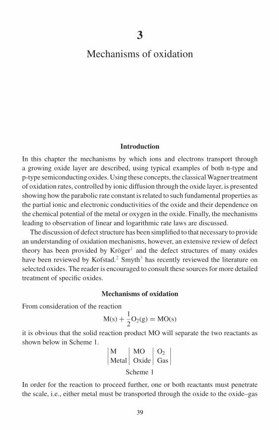
3
Mechanisms of oxidation
Introduction
In this chapter the mechanisms by which ions and electrons transport througha growing oxide layer are described, using typical examples of both n-type andp-type semiconducting oxides. Using these concepts, the classical Wagner treatmentof oxidation rates, controlled by ionic diffusion through the oxide layer, is presentedshowing how the parabolic rate constant is related to such fundamental properties asthe partial ionic and electronic conductivities of the oxide and their dependence onthe chemical potential of the metal or oxygen in the oxide. Finally, the mechanismsleading to observation of linear and logarithmic rate laws are discussed.
The discussion of defect structure has been simplified to that necessary to providean understanding of oxidation mechanisms, however, an extensive review of defecttheory has been provided by Kroger1 and the defect structures of many oxideshave been reviewed by Kofstad.2 Smyth3 has recently reviewed the literature onselected oxides. The reader is encouraged to consult these sources for more detailedtreatment of specific oxides.
Mechanisms of oxidation
From consideration of the reaction
M(s) + 1
2O2(g) = MO(s)
it is obvious that the solid reaction product MO will separate the two reactants asshown below in Scheme 1. ∣∣∣∣M
Metal
∣∣∣∣ MOOxide
∣∣∣∣ O2
Gas
∣∣∣∣Scheme 1
In order for the reaction to proceed further, one or both reactants must penetratethe scale, i.e., either metal must be transported through the oxide to the oxide–gas
39
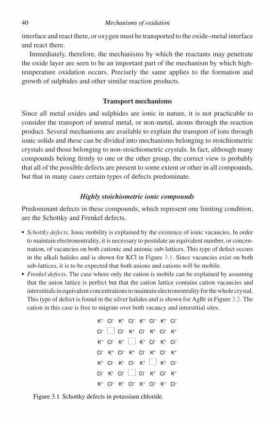
40 Mechanisms of oxidation
interface and react there, or oxygen must be transported to the oxide–metal interfaceand react there.
Immediately, therefore, the mechanisms by which the reactants may penetratethe oxide layer are seen to be an important part of the mechanism by which high-temperature oxidation occurs. Precisely the same applies to the formation andgrowth of sulphides and other similar reaction products.
Transport mechanisms
Since all metal oxides and sulphides are ionic in nature, it is not practicable toconsider the transport of neutral metal, or non-metal, atoms through the reactionproduct. Several mechanisms are available to explain the transport of ions throughionic solids and these can be divided into mechanisms belonging to stoichiometriccrystals and those belonging to non-stoichiometric crystals. In fact, although manycompounds belong firmly to one or the other group, the correct view is probablythat all of the possible defects are present to some extent or other in all compounds,but that in many cases certain types of defects predominate.
Highly stoichiometric ionic compounds
Predominant defects in these compounds, which represent one limiting condition,are the Schottky and Frenkel defects.
� Schottky defects. Ionic mobility is explained by the existence of ionic vacancies. In orderto maintain electroneutrality, it is necessary to postulate an equivalent number, or concen-tration, of vacancies on both cationic and anionic sub-lattices. This type of defect occursin the alkali halides and is shown for KCl in Figure 3.1. Since vacancies exist on bothsub-lattices, it is to be expected that both anions and cations will be mobile.
� Frenkel defects. The case where only the cation is mobile can be explained by assumingthat the anion lattice is perfect but that the cation lattice contains cation vacancies andinterstitials in equivalent concentrations to maintain electroneutrality for the whole crystal.This type of defect is found in the silver halides and is shown for AgBr in Figure 3.2. Thecation in this case is free to migrate over both vacancy and interstitial sites.
K+ Cl− Cl− Cl− Cl−
Cl−Cl−Cl−Cl−
Cl− Cl− Cl−
Cl− Cl− Cl− Cl−
Cl−Cl−Cl−
Cl− Cl− Cl− Cl−
Cl− Cl− Cl− Cl−
K+ K+ K+
K+ K+ K+
K+
K+ K+ K+ K+
K+ K+ K+ K+
K+ K+
K+ K+ K+ K+
K+
K+ K+ K+
Figure 3.1 Schottky defects in potassium chloride.
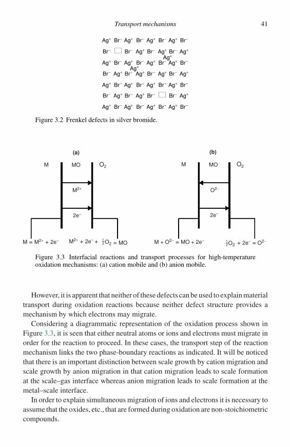
Transport mechanisms 41
Ag+ Br− Br− Br− Br−
Br−Br−Br−Br−
Br− Br− Br− Br−
Br−Br−Br−Br−
Br− Br− Br− Br−
Br−Br−Br−Br−
Br− Br− Br− Br−
Ag+ Ag+ Ag+
Ag+Ag+Ag+
Ag+
Ag+ Ag+
Ag+Ag+ Ag+
Ag+Ag+Ag+Ag+
Ag+ Ag+ Ag+ Ag+
Ag+Ag+Ag+
Ag+ Ag+ Ag+ Ag+
Figure 3.2 Frenkel defects in silver bromide.
(a) (b)
MOM O2 MOM O2
M2+ O2−
2e− 2e−
M = M2+ + 2e− M2+ + 2e− + 12 O2 = MO M + O2− = MO + 2e− 1
2O2 + 2e− = O2−
Figure 3.3 Interfacial reactions and transport processes for high-temperatureoxidation mechanisms: (a) cation mobile and (b) anion mobile.
However, it is apparent that neither of these defects can be used to explain materialtransport during oxidation reactions because neither defect structure provides amechanism by which electrons may migrate.
Considering a diagrammatic representation of the oxidation process shown inFigure 3.3, it is seen that either neutral atoms or ions and electrons must migrate inorder for the reaction to proceed. In these cases, the transport step of the reactionmechanism links the two phase-boundary reactions as indicated. It will be noticedthat there is an important distinction between scale growth by cation migration andscale growth by anion migration in that cation migration leads to scale formationat the scale–gas interface whereas anion migration leads to scale formation at themetal–scale interface.
In order to explain simultaneous migration of ions and electrons it is necessary toassume that the oxides, etc., that are formed during oxidation are non-stoichiometriccompounds.
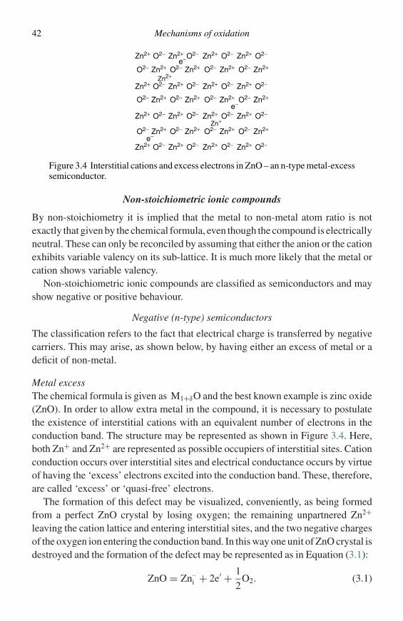
42 Mechanisms of oxidation
Zn2+ Zn2+
Zn2+
Zn2+
Zn2+
Zn2+Zn2+
Zn2+
Zn2+
Zn2+ Zn2+
Zn2+ Zn2+ Zn2+ Zn2+
Zn2+
Zn+Zn2+Zn2+Zn2+
Zn2+
Zn2+
Zn2+ Zn2+ Zn2+
Zn2+ Zn2+Zn2+
Zn2+
Zn2+
O2−O2−e−
e−
e−
O2−
O2−
O2−
O2−
O2− O2− O2− O2−
O2−O2−
O2− O2− O2− O2−
O2−O2−O2−O2−
O2− O2−
O2−
O2−
O2−
O2−O2−
O2−
Figure 3.4 Interstitial cations and excess electrons in ZnO – an n-type metal-excesssemiconductor.
Non-stoichiometric ionic compounds
By non-stoichiometry it is implied that the metal to non-metal atom ratio is notexactly that given by the chemical formula, even though the compound is electricallyneutral. These can only be reconciled by assuming that either the anion or the cationexhibits variable valency on its sub-lattice. It is much more likely that the metal orcation shows variable valency.
Non-stoichiometric ionic compounds are classified as semiconductors and mayshow negative or positive behaviour.
Negative (n-type) semiconductors
The classification refers to the fact that electrical charge is transferred by negativecarriers. This may arise, as shown below, by having either an excess of metal or adeficit of non-metal.
Metal excessThe chemical formula is given as M1+δO and the best known example is zinc oxide(ZnO). In order to allow extra metal in the compound, it is necessary to postulatethe existence of interstitial cations with an equivalent number of electrons in theconduction band. The structure may be represented as shown in Figure 3.4. Here,both Zn+ and Zn2+ are represented as possible occupiers of interstitial sites. Cationconduction occurs over interstitial sites and electrical conductance occurs by virtueof having the ‘excess’ electrons excited into the conduction band. These, therefore,are called ‘excess’ or ‘quasi-free’ electrons.
The formation of this defect may be visualized, conveniently, as being formedfrom a perfect ZnO crystal by losing oxygen; the remaining unpartnered Zn2+
leaving the cation lattice and entering interstitial sites, and the two negative chargesof the oxygen ion entering the conduction band. In this way one unit of ZnO crystal isdestroyed and the formation of the defect may be represented as in Equation (3.1):
ZnO = Zn··i + 2e′ + 1
2O2. (3.1)
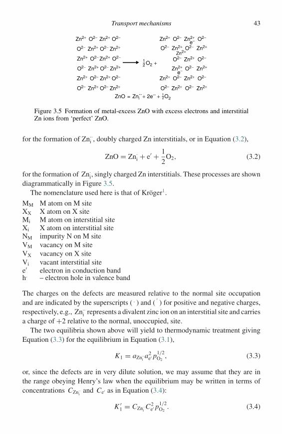
Transport mechanisms 43
12ZnO = Zni + 2e− +
Zn2+
Zn2+ Zn2+O2− O2−
Zn2+ Zn2+O2−O2−
Zn2+ Zn2+O2− O2−
Zn2+Zn2+ O2−O2−
Zn2+ Zn2+O2− O2−
e−
e−
Zn2+ Zn2+O2−O2−
Zn2+ Zn2+O2− O2−
Zn2+ Zn2+O2− O2−
Zn2+ O2−O2−
Zn2+ Zn2+O2−
Zn2+ Zn2+O2− O2−
Zn2+Zn2+ O2−O2−
O2
12 O2 +
:
Figure 3.5 Formation of metal-excess ZnO with excess electrons and interstitialZn ions from ‘perfect’ ZnO.
for the formation of Zn··i , doubly charged Zn interstitials, or in Equation (3.2),
ZnO = Zn·i + e′ + 1
2O2, (3.2)
for the formation of Zn·i, singly charged Zn interstitials. These processes are shown
diagrammatically in Figure 3.5.The nomenclature used here is that of Kroger1.
MM M atom on M siteXX X atom on X siteMi M atom on interstitial siteXi X atom on interstitial siteNM impurity N on M siteVM vacancy on M siteVX vacancy on X siteVi vacant interstitial sitee′ electron in conduction bandh. – electron hole in valence band
The charges on the defects are measured relative to the normal site occupationand are indicated by the superscripts ( . ) and (
′) for positive and negative charges,
respectively, e.g., Zn··i represents a divalent zinc ion on an interstitial site and carries
a charge of +2 relative to the normal, unoccupied, site.The two equilibria shown above will yield to thermodynamic treatment giving
Equation (3.3) for the equilibrium in Equation (3.1),
K1 = aZn··ia2
e′ p1/2O2
, (3.3)
or, since the defects are in very dilute solution, we may assume that they are inthe range obeying Henry’s law when the equilibrium may be written in terms ofconcentrations CZn··
iand Ce′ as in Equation (3.4):
K ′1 = CZn··
iC2
e′ p1/2O2
. (3.4)
44 Mechanisms of oxidation
If Equation (3.1) represents the only mechanism by which defects are created inZnO, then Equation (3.5) follows:
2CZn··i= Ce′ . (3.5)
Hence, putting Equation (3.5) into Equation (3.4), we obtain Equation (3.6a),
K ′1 = 4C3
Zn··ip1/2
O2, (3.6a)
or Equation (3.6b), and therefore we obtain Equation (3.7):
CZn··i= (K ′
1/4)1/3 p−1/6O2
= const.p−1/6O2
, (3.6b)
Ce′ ∝ p−1/6O2
. (3.7)
Similarly, applying the same analysis to the reaction shown in Equation (3.2) theresult shown in Equation (3.8) is obtained:
CZn·i= Ce′ ∝ p−1/4
O2. (3.8)
Clearly each mechanism predicts a different dependence of defect concentration onoxygen partial pressure. Since the electrical conductivity depends on the concen-tration of conduction-band electrons, measurement of electrical conductivity as afunction of oxygen partial pressure should serve to define the dependence law andindicate which defect is predominant. Initial experiments of this type carried outbetween 500 and 700 ◦C4 indicated that the conductivity varied with oxygen partialpressure having exponents between 1/4.5 and 1/5. This indicates that neither defectmechanism predominates, and the actual structure could involve both singly anddoubly charged interstitial cations.2
More recent work has confirmed that significant interstitial solution of zinc occursin ZnO. The results of various studies have been interpreted in terms of neutral zincinterstitial atoms5 and singly charged interstitial ions.6,7 The latter are favouredpresently, although it has also been suggested, on the basis of oxygen diffusionmeasurements, that oxygen vacancies are important above 1000 ◦C.8 Kofstad2
concludes that no overall consistent interpretation can be made regarding ZnO.Inconsistencies between different investigations concerning the establishment
of defect structures can frequently result from impurities in the sample, especiallyin the case of compounds which show only slight deviations from stoichiometry.As the purity of available materials improves, it would be prudent to repeat suchmeasurements.
Non-metal deficit
Alternatively, n-type behaviour can be caused by non-metal deficit, as men-tioned above. For oxides, this may be visualised as the discharge and subsequent
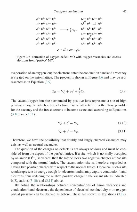
Transport mechanisms 45
12 O2 +
O2− O2−M2+ M2+
M2+M2+ O2−O2−
M2+ M2+O2− O2−
M2+M2+ O2−O2−
M2+ M2+O2− O2−
M2+ M2+O2−O2−
M2+ M2+O2− O2−
M2+M2+ O2− O2−
M2+ M2+O2−O2−
M2+M2+ O2− O2−
M2+ M2+O2−O2−
OO = VO + 2e− +
e−
e−
M2+ M2+O2−
12 O2
:
Figure 3.6 Formation of oxygen-deficit MO with oxygen vacancies and excesselectrons from ‘perfect’ MO.
evaporation of an oxygen ion; the electrons enter the conduction band and a vacancyis created on the anion lattice. The process is shown in Figure 3.6 and may be rep-resented as in Equation (3.9):
OO = V··O + 2e′ + 1
2O2. (3.9)
The vacant oxygen-ion site surrounded by positive ions represents a site of highpositive charge to which a free electron may be attracted. It is therefore possiblefor the vacancy and the free electrons to become associated according to Equations(3.10) and (3.11):
V··O + e′ = V·
O, (3.10)
V·O + e′ = VO. (3.11)
Therefore, we have the possibility that doubly and singly charged vacancies mayexist as well as neutral vacancies.
The question of the charges on defects is not always obvious and must be con-sidered from the aspect of the perfect lattice. If a site, which is normally occupiedby an anion (O2−), is vacant, then the lattice lacks two negative charges at that sitecompared with the normal lattice. The vacant anion site is, therefore, regarded ashaving two positive charges with respect to the normal lattice. Of course, such a sitewould represent an energy trough for electrons and so may capture conduction-bandelectrons, thus reducing the relative positive charge in the vacant site as indicatedin Equations (3.10) and (3.11) above.
By noting the relationships between concentrations of anion vacancies andconduction-band electrons, the dependence of electrical conductivity κ on oxygenpartial pressure can be derived as before. These are shown in Equations (3.12),
46 Mechanisms of oxidation
(3.13), and (3.14) for the doubly charged, singly charged, and neutral vacancies,respectively:
κ ∝ Ce′ ∝ p−1/6O2
, (3.12)
κ ∝ Ce′ ∝ p−1/4O2
(3.13)
κ ∝ Ce′ (independent of pO2). (3.14)
Notice that in Equations (3.7), (3.8), (3.12), and (3.13) the power of the oxygenpartial pressure is negative. This is the case for all n-type semiconductors.
Positive (p-type) semiconductors
In this case charge is transferred by positive carriers. This may arise from either adeficit of metal or an excess of non-metal.
Metal deficit
Positive (p-type) semiconduction arises from the formation of vacancies on thecation lattice together with electron holes, giving rise to conduction. The formulamay be written M1−δO. The value of δ can vary widely; from 0.05 in the case ofFe0.95O (wustite), 0.001 for NiO, to very small deviations in the case of Cr2O3 andAl2O3.
The possibility of forming electron holes lies in the ability of many metal ions,especially of the ions of transition metals, to exist in several valence states. Thecloser together the different valence states are in terms of energy of ionization, themore easily can cation vacancy formation be induced by the metal-deficit p-typemechanism.
The typical structure of this class of oxides is represented in Figure 3.7 takingNiO as an example. By virtue of the energetically close valence states of the cationit is relatively easy for an electron to transfer from a Ni2+ to a Ni3+ thus reversingthe charges on the two ions. The site Ni3+ is thus seen to offer a low-energy positionfor an electron and is called an ‘electron hole’.
The formation of this defect structure can easily be visualized if one considersthe interaction of the NiO lattice with oxygen shown in Figure 3.8.
In step (b) the oxygen chemisorbs by attracting an electron from a Ni site thusforming a Ni3+ or hole. In step (c) the chemisorbed oxygen is fully ionized forminganother hole and a Ni2+ ion enters the surface to partner the O2−, thus forming avacancy in the cation sub-lattice. Note that this process also forms an extra unitof NiO on the surface of the oxide, which should reflect in density changes ifsufficiently sensitive measurements were made.
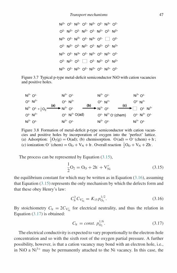
Transport mechanisms 47
Ni2+ Ni2+ Ni2+
Ni2+ Ni2+ Ni2+ Ni2+
Ni2+Ni2+
Ni2+ Ni2+ Ni2+ Ni3+
Ni2+Ni2+Ni2+
Ni2+ Ni2+ Ni2+
Ni2+Ni2+Ni2+
Ni3+
Ni3+
Ni3+
Ni2+
O2− O2− O2− O2−
O2−O2−O2−O2−
O2− O2− O2− O2−
O2− O2−O2−O2−
O2− O2− O2− O2−
O2−O2−O2−O2−
O2− O2− O2− O2−
Figure 3.7 Typical p-type metal-deficit semiconductor NiO with cation vacanciesand positive holes.
Ni2+
Ni2+
Ni2+
Ni2+
Ni2+
Ni2+
Ni2+
Ni2+
Ni2+ Ni2+
Ni3+
Ni3+
Ni3+ Ni2+
Ni2+
Ni2+
Ni2+
Ni2+
Ni2+
Ni2+
O2−
O2−
O2−
O2−
O2−
O2−
O2−
O2−
O2−
O2−
O2−
O2−
O2−
O2−
O2−O2−
O2− O−(chem)O(ad) O2− O2−
O2−O2−
12 O2 +
(a) (b) (c)
Figure 3.8 Formation of metal-deficit p-type semiconductor with cation vacan-cies and positive holes by incorporation of oxygen into the ‘perfect’ lattice.(a) Adsorption: 1
2 O2(g) = O(ad); (b) chemisorption. O (ad) = O−(chem) + h.;(c) ionization: O−(chem) = OO + VN + h.. Overall reaction 1
2 OO + VN + Zh..
The process can be represented by Equation (3.15),
1
2O2 = OO + 2h· + V′′
Ni (3.15)
the equilibrium constant for which may be written as in Equation (3.16), assumingthat Equation (3.15) represents the only mechanism by which the defects form andthat these obey Henry’s law:
C2h·CV′′
Ni= K15 p1/2
O2. (3.16)
By stoichiometry Ch· = 2CV′′Ni
for electrical neutrality, and thus the relation inEquation (3.17) is obtained:
Ch· = const. p1/6O2
. (3.17)
The electrical conductivity is expected to vary proportionally to the electron-holeconcentration and so with the sixth root of the oxygen partial pressure. A furtherpossibility, however, is that a cation vacancy may bond with an electron hole, i.e.,in NiO a Ni3+ may be permanently attached to the Ni vacancy. In this case, the
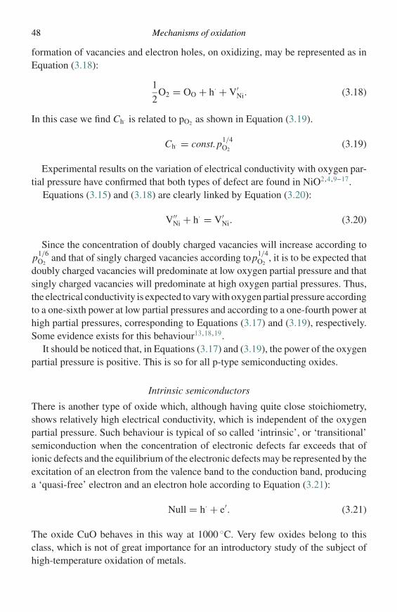
48 Mechanisms of oxidation
formation of vacancies and electron holes, on oxidizing, may be represented as inEquation (3.18):
1
2O2 = OO + h· + V′
Ni. (3.18)
In this case we find Ch· is related to pO2 as shown in Equation (3.19).
Ch· = const.p1/4O2
(3.19)
Experimental results on the variation of electrical conductivity with oxygen par-tial pressure have confirmed that both types of defect are found in NiO2,4,9–17.
Equations (3.15) and (3.18) are clearly linked by Equation (3.20):
V′′Ni + h· = V′
Ni. (3.20)
Since the concentration of doubly charged vacancies will increase according top1/6
O2and that of singly charged vacancies according top1/4
O2, it is to be expected that
doubly charged vacancies will predominate at low oxygen partial pressure and thatsingly charged vacancies will predominate at high oxygen partial pressures. Thus,the electrical conductivity is expected to vary with oxygen partial pressure accordingto a one-sixth power at low partial pressures and according to a one-fourth power athigh partial pressures, corresponding to Equations (3.17) and (3.19), respectively.Some evidence exists for this behaviour13,18,19.
It should be noticed that, in Equations (3.17) and (3.19), the power of the oxygenpartial pressure is positive. This is so for all p-type semiconducting oxides.
Intrinsic semiconductors
There is another type of oxide which, although having quite close stoichiometry,shows relatively high electrical conductivity, which is independent of the oxygenpartial pressure. Such behaviour is typical of so called ‘intrinsic’, or ‘transitional’semiconduction when the concentration of electronic defects far exceeds that ofionic defects and the equilibrium of the electronic defects may be represented by theexcitation of an electron from the valence band to the conduction band, producinga ‘quasi-free’ electron and an electron hole according to Equation (3.21):
Null = h· + e′. (3.21)
The oxide CuO behaves in this way at 1000 ◦C. Very few oxides belong to thisclass, which is not of great importance for an introductory study of the subject ofhigh-temperature oxidation of metals.
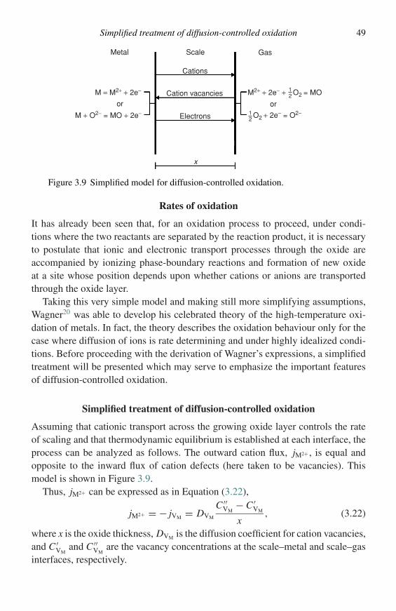
Simplified treatment of diffusion-controlled oxidation 49
Metal Scale Gas
Cations
Cation vacancies
Electrons
x
M = M2+ + 2e−
or
M + O2− = MO + 2e−
M2+ + 2e− + = MO12 O2
12
O2 + 2e− = O2− or
Figure 3.9 Simplified model for diffusion-controlled oxidation.
Rates of oxidation
It has already been seen that, for an oxidation process to proceed, under condi-tions where the two reactants are separated by the reaction product, it is necessaryto postulate that ionic and electronic transport processes through the oxide areaccompanied by ionizing phase-boundary reactions and formation of new oxideat a site whose position depends upon whether cations or anions are transportedthrough the oxide layer.
Taking this very simple model and making still more simplifying assumptions,Wagner20 was able to develop his celebrated theory of the high-temperature oxi-dation of metals. In fact, the theory describes the oxidation behaviour only for thecase where diffusion of ions is rate determining and under highly idealized condi-tions. Before proceeding with the derivation of Wagner’s expressions, a simplifiedtreatment will be presented which may serve to emphasize the important featuresof diffusion-controlled oxidation.
Simplified treatment of diffusion-controlled oxidation
Assuming that cationic transport across the growing oxide layer controls the rateof scaling and that thermodynamic equilibrium is established at each interface, theprocess can be analyzed as follows. The outward cation flux, jM2+ , is equal andopposite to the inward flux of cation defects (here taken to be vacancies). Thismodel is shown in Figure 3.9.
Thus, jM2+ can be expressed as in Equation (3.22),
jM2+ = − jVM = DVM
C ′′VM
− C ′VM
x, (3.22)
where x is the oxide thickness, DVM is the diffusion coefficient for cation vacancies,and C ′
VMand C ′′
VMare the vacancy concentrations at the scale–metal and scale–gas
interfaces, respectively.
50 Mechanisms of oxidation
Since there is thermodynamic equilibrium at each interface, the value of(C ′′
VM− C ′
VM) is constant and we have Equation (3.23),
jM2+ = 1
Vox
dx
dt= DVM
C ′′VM
− C ′VM
x, (3.23)
i.e., the rate of oxide thickening is given in Equation (3.24),
dx
dt= k ′
xwhere k ′ = DVM Vox(C ′′
VM− C ′
VM), (3.24)
where Vox is the molar volume of the oxide. Integrating and noting that x = 0 att = 0 we obtain Equation (3.25),
x2 = 2k ′t, (3.25)
which is the common parabolic rate law.Furthermore, since it has been shown that the cation-vacancy concentration is
related to the oxygen partial pressure by Equation (3.26),
CVM = const.p1/nO2
,
the variation of the parabolic rate constant with oxygen partial pressure can bepredicted, i.e., Equation (3.26):
k ′ ∝ [(p′′
O2
)1/n − (p′
O2
)1/n]. (3.26)
Since p′O2
is usually negligible compared with p′′O2
we have Equation (3.27):
k ′ ∝ (p′′
O2
)1/n. (3.27)
Wagner theory of oxidation20
Figure 3.10 gives a summary of the conditions, later stated, for which the theory isvalid. Assumptions are listed below.
(1) The oxide layer is a compact, perfectly adherent scale.(2) Migration of ions or electrons across the scale is the rate-controlling process.(3) Thermodynamic equilibrium is established at both the metal–scale and scale–gas inter-
faces.(4) The oxide scale shows only small deviations from stoichiometry and, hence, the ionic
fluxes are independent of position within the scale.(5) Thermodynamic equilibrium is established locally throughout the scale.(6) The scale is thick compared with the distances over which space charge effects (electrical
double layer) occur.(7) Oxygen solubility in the metal may be neglected.
Since thermodynamic equilibrium is assumed to be established at the metal–scale and scale–gas interfaces, it follows that activity gradients of both metal and
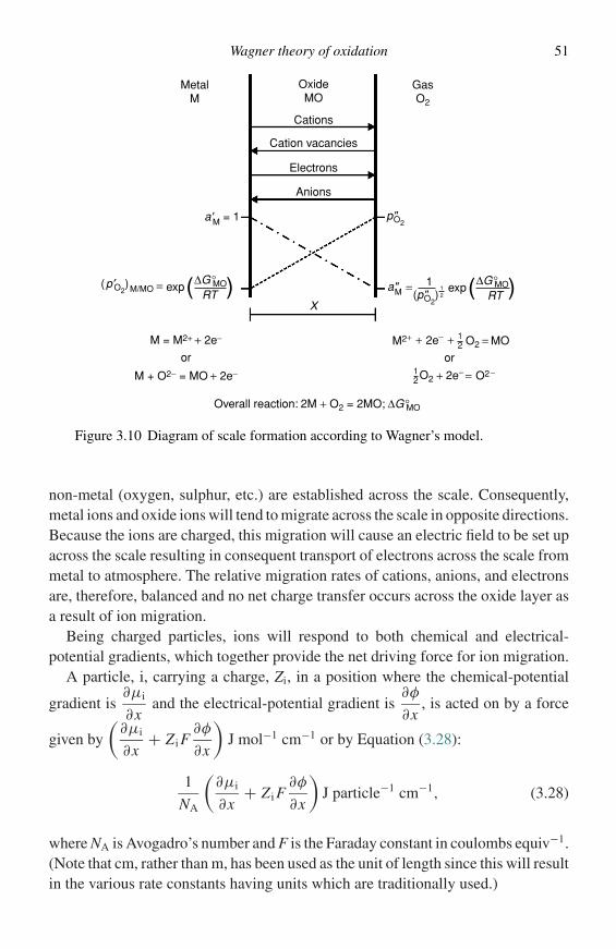
Wagner theory of oxidation 51
MetalM
OxideMO
Cations
Cation vacancies
Electrons
Anions
p"O2
(p"O2)
∆G°MO
M2+
O2−
2e−
2e−
O2 MO
or
RTa"M
GasO2
1 exp( )(p ′O2)M/MO
∆G°MORT
exp( )
+
+
+ =
==
=
12
12
O212
M = M2+ + 2e−
M + O2− = MO + 2e−
or
Overall reaction: 2M + O2 = 2MO; ∆G°MO
a'M = 1
X
Figure 3.10 Diagram of scale formation according to Wagner’s model.
non-metal (oxygen, sulphur, etc.) are established across the scale. Consequently,metal ions and oxide ions will tend to migrate across the scale in opposite directions.Because the ions are charged, this migration will cause an electric field to be set upacross the scale resulting in consequent transport of electrons across the scale frommetal to atmosphere. The relative migration rates of cations, anions, and electronsare, therefore, balanced and no net charge transfer occurs across the oxide layer asa result of ion migration.
Being charged particles, ions will respond to both chemical and electrical-potential gradients, which together provide the net driving force for ion migration.
A particle, i, carrying a charge, Zi, in a position where the chemical-potential
gradient is∂µi
∂xand the electrical-potential gradient is
∂φ
∂x, is acted on by a force
given by
(∂µi
∂x+ Z i F
∂φ
∂x
)J mol−1 cm−1 or by Equation (3.28):
1
NA
(∂µi
∂x+ Z i F
∂φ
∂x
)J particle−1 cm−1, (3.28)
where NA is Avogadro’s number and F is the Faraday constant in coulombs equiv−1.(Note that cm, rather than m, has been used as the unit of length since this will resultin the various rate constants having units which are traditionally used.)
52 Mechanisms of oxidation
The application of a force to a particle i leads to a drift velocity, vi (cm s−1),which is proportional to the acting force, hence for the force in Equation (3.28),
vi = − Bi
NA
(∂µi
∂x+ Z i F
∂φ
∂x
), (3.29)
where Bi is the particle mobility and is defined as the average drift velocity per unitforce, particle cm2 J−1 s−1. The negative sign in the equation arises since the driftvelocity takes place in the positive x direction for negative chemical and electricalpotential gradients. The flux of particles is obtained as in Equation (3.30),
ji = Civi = −Ci Bi
NA
(∂µi
∂x+ Z i F
∂φ
∂x
)mol cm−2 s−1 (3.30)
where Ci is the concentration of i in mol cm−3.The mobility may be related to the conductivity κi and the self diffusion coef-
ficient Di of the particle by comparing Equation (3.30) for limiting cases of zeroelectrical-potential gradient and zero chemical-potential gradient to Fick’s first lawand Ohm’s law, respectively. The relationships in Equation (3.31) are obtained,
kBT Bi = Di = RT κi
Ci(Z i F)2(3.31)
where kB is Boltzmann’s constant. Upon using Equation (3.31) to replace the mobil-ity Bi in Equation (3.30) with the partial conductivity one has Equation (3.32):
ji = − κi
Z2i F2
(∂µi
∂x+ Z i F
∂φ
∂x
)(3.32)
Equation (3.32) can be used to describe the flux of cations, anions, or electronsthrough the oxide layer. Due to their different mobilities, different species wouldtend to move at different rates, however, this would set up electric fields tending tooppose this independence. In fact, the three species migrate at rates that are definedby the necessity of maintaining electroneutrality throughout the scale, i.e, such thatthere is no net charge across the oxide scale. This condition is usually achieved dueto the very high mobility of electrons or electronic defects.
The original treatment by Wagner involved cations, anions, and electrons. How-ever, the majority of oxides and sulphides show high electronic mobility, and themobilities of the cation and anion species usually differ by several orders of mag-nitude. It is, therefore, possible to ignore the migration of the slower-moving ionicspecies and thus simplify the treatment somewhat.
The most frequently met case involves oxides and sulphides in which cationsand electrons are the mobile species. Writing Zc and Ze for the charges on cationsand electrons respectively, and using Equation (3.32), we have the respective fluxes
Wagner theory of oxidation 53
given in Equations (3.33) and (3.34):
jc = − κc
Z2c F2
(∂µc
∂x+ Zc F
∂φ
∂x
), (3.33)
je = − κe
Z2e F2
(∂µe
∂x+ Ze F
∂φ
∂x
). (3.34)
The condition for electrical neutrality is given by Equation (3.35),
Zc jc + Ze je = 0, (3.35)
and, using Equations (3.33)–(3.35), it is now possible to eliminate∂φ
∂xas Equation
(3.36):
∂φ
∂x= − 1
F(κc + κe)
[κc
Zc
∂µc
∂x+ κe
Ze
∂µe
∂x
]. (3.36)
Substituting Equation (3.36) in Equation (3.33) we have for the flux of cationsEquation (3.37).
jc = − κcκe
Z2c F2(κc + κe)
[∂µc
∂x− Zc
Ze
∂µe
∂x
]. (3.37)
Since the electronic charge Ze = −1, Equation (3.37) becomes Equation (3.38):
jc = − κcκe
Z2c F2(κc + κe)
[∂µc
∂x+ Zc
∂µe
∂x
]. (3.38)
The ionization of a metal M is represented by M = MZc+ + Zce, and it follows that,at equilibrium, we have the relation given in Equation (3.39):
µM = µc + Zcµe. (3.39)
Therefore, from Equations (3.38) and (3.39), Equation (3.40) is obtained:
jc = − κcκe
Z2c F2(κc + κe)
∂µM
∂x. (3.40)
Equation (3.40) is the expression for the cationic flux at any place in the scale where
κc, κe, and∂µM
∂xare the instantaneous values at that place. Since all of these values
may change with the position in the scale, it is necessary to integrate Equation (3.40)in order to define jc in terms of the scale thickness and the measurable metal chemicalpotentials at the metal–scale, µ′
M, and scale–gas, µ′′M, interfaces. For phases with
small deviations from stoichiometry, jc can be assumed to be independent of x,
54 Mechanisms of oxidation
hence defined by Equation (3.41a) or (3.41b),
jc
∫ x
0dx = − 1
Z2c F2
∫ µ′′M
µ′M
κcκe
κc + κedµM, (3.41a)
jc = − 1
Z2c F2x
∫ µ′′M
µ′M
κcκe
κc + κedµM mol cm2 s−1. (3.41b)
and, using Equation (3.35), Equation (3.42) is obtained:
je = − 1
Zc F2x
∫ µ′′M
µ′M
κcκe
κc + κedµM mol cm−2 s−1. (3.42)
If the concentration of metal in the oxide scale is CM mol cm−3 then the flux mayalso be expressed by Equation (3.43),
jc = CMdx
dt, (3.43)
where x is the oxide-scale thickness.The parabolic rate law is usually expressed by Equation (3.24), where k ′ is the
parabolic rate constant in cm2 s−1.Comparing Equations (3.41), (3.43), and (3.24), the parabolic rate constant is
expressed by Equation (3.44):
k ′ = 1
Z2c F2CM
∫ µ′M
µ′′M
κcκe
κc + κedµM. (3.44)
A similar treatment for the case where anions are more mobile than cations, i.e.,the migration of cations may be neglected, yields Equation (3.45),
k ′ = 1
Z2a F2CX
∫ µ′′X
µ′X
κaκe
κa + κedµX, (3.45)
where κa is the partial electrical conductivity of the anions and X is the non-metal,oxygen, or sulphur.
In general, it is found that the transport number of electrons, or electronic defects,is close to unity, compared with which the transport numbers of cations or anionsare negligibly small. In these cases, Equations (3.44) and (3.45) reduce to Equations(3.46) and (3.47), respectively:
k ′ = 1
Z2c F2CM
∫ µ′M
µ′′M
κcdµM cm2 s−1, (3.46)
k ′ = 1
Z2a F2CX
∫ µ′′X
µ′X
κadµX cm2 s−1. (3.47)
Wagner theory of oxidation 55
Using Equations (3.31), and (3.46), one has Equations (3.48) and (3.49),
k ′ = 1
RT
∫ µ′M
µ′′M
DMdµM cm2 s−1, (3.48)
k ′ = 1
RT
∫ µ′′X
µ′X
DXdµX cm2 s−1, (3.49)
for the parabolic rate constant, where DM and DX are the diffusion coefficients formetal, M, and non-metal, X, through the scale, respectively.
Equations (3.48) and (3.49) are written in terms of variables that can be measuredrelatively easily, although it is assumed that the diffusion coefficient is a function ofthe chemical potential of the species involved. Thus, in order to be able to calculatevalues of the parabolic rate constant, the relevant diffusion coefficient must beknown as a function of the chemical potential of the mobile species. Such dataare frequently not available or are incomplete. Furthermore, it is usually easier tomeasure the parabolic rate constant directly than to carry out experiments to measurethe diffusion data. Thus, the real value of Wagner’s analysis lies in providing acomplete mechanistic understanding of the process of high-temperature oxidationunder the conditions set out.
The predictions of Wagner’s theory for n-type and p-type oxides in which cationsare the mobile species should now be examined. The first class is represented byZnO which is formed by the oxidation of zinc.
The defect structure of zinc oxide involves interstitial zinc ions and excess orquasi-free electrons according to Equations (3.1) and (3.2):
ZnO = Zn··i + 2e′ + 1
2O2, (3.1)
ZnO = Zn·i + e′ + 1
2O2. (3.2)
The partial conductivity of interstitial zinc ions is expected to vary with theirconcentration. As shown before, it is expected that this will vary according to theoxygen partial pressure, as shown in Equations (3.50) and (3.51),
κZn··i∝ CZn··
i∝ p−1/6
O2, (3.50)
CZn·i∝ p−1/4
O2, (3.51)
i.e, κZn··i
and κZn·ican be defined as in Equations (3.52) and (3.53):
κZn··i= const.p−1/6
O2, (3.52)
κZn·i= const.p−1/4
O2. (3.53)
56 Mechanisms of oxidation
Since ZnO shows only small deviations from stoichiometry we can write Equa-tion (3.54):
µZn + µO = µZnO ≈ constant; (3.54)
also, µO may be expressed by Equation (3.55):
µO = 1
2µo
O2+ 1
2RT ln pO2 . (3.55)
Therefore we obtain Equations (3.56a) (3.56b):
0 = dµZn + 1
2RT d ln pO2, (3.56a)
dµZn = −1
2RT d ln pO2 . (3.56b)
Using Equations (3.46), (3.52), and (3.56b) we obtain Equation (3.57a):
k ′ZnO = −const.
∫ p′O2
p′′O2
p−1/6O2
d ln pO2 = −const.∫ p′
O2
p′′O2
p−7/6O2
dpO2, (3.57a)
which, upon integration, yields Equation (3.57b):
k ′ZnO = const.′′
(
1
p′O2
)1/6
−(
1
p′′O2
)1/6 . (3.57b)
Alternatively, using Equations (3.46), (3.53), and (3.56) we obtain Equation (3.58):
k ′ZnO = const.′′
(
1
p′O2
)1/4
−(
1
p′′O2
)1/4 (3.58)
Generally p′′O2
is much greater than p′O2
and so the parabolic rate constant for zincis expected to be practically independent of the externally applied oxygen partialpressure, regardless of the relative abundances of Zn··
i and Zn·i.
A similar treatment can be applied to the oxidation of cobalt to CoO. Cobaltmonoxide is a metal deficit p-type semiconductor forming cation vacancies andelectron holes21,22 according to Equation (3.59), where K59 = CV′
CoCh· p−1/2
O2:
1
2O2 = OO + V ′
Co + h·. (3.59)
Excluding defects caused by impurities and any contribution from intrinsic elec-tronic defects we see from Equation (3.59) that, in order to satisfy both stoichiometryand electroneutrality, we have the relation shown in Equation (3.60):
CV′Co
= Ch· ∝ p1/4O2
, (3.60)
Wagner theory of oxidation 57
and consequently the cationic partial conductivity is given by Equation (3.61):
κCo ∝ p1/4O2
. (3.61)
Thus, substituting Equation (3.61) into Equation (3.46), we obtain Equation (3.62)for the parabolic scaling constant (for Co being oxidized to CoO):
k ′CoO ∝
∫ p′′O2
p′O2
p1/4O2
d ln pO2 . (3.62a)
Alternatively we can have Equation (3.62b),
k ′CoO ∝
∫ p′′O2
p′O2
p−3/4O2
dpO2, (3.62b)
and integrating obtain Equation (3.63):
k ′CoO ∝
[(p′′
O2
)1/4 − (p′
O2
)1/4]. (3.63)
In Equation (3.63) the value of p′O2
for the equilibrium between Co and CoOcan be neglected compared with the value of p′′
O2in the atmosphere. This is valid
because diffusion control of the oxidation reaction rate is achieved only underconditions where p′′
O2is sufficiently high to avoid control of the reaction rate by
surface reactions or transport through the gas phase.Under this assumption, Equation (3.63) simplifies to Equation (3.64).
k ′CoO ∝ (
p′′O2
)1/4(3.64)
The existence of doubly charged cation vacancies might also be postulated accord-ing to Equation (3.65),
1
2O2 = OO + V ′′
Co + 2h·, (3.65)
for which K65 is expressed by Equation (3.66):
K65 = CV′′Co
C2h· p
−1/2O2
. (3.66)
If these defects were predominant then, following the same argument, the parabolicrate constant for oxidation of cobalt would be expected to vary with oxygen partialpressure as in Equation (3.67):
k ′CoO ∝ (
p′′O2
)1/6. (3.67)
Measurements of the electrical conductivity of CoO as a function of oxygenpartial pressure by Fisher and Tannhauser21 show that the doubly charged vacancymodel according to Equation (3.65) is obeyed up to values of oxygen partial pressurein the region of 10−5 atm. Above this value the singly charged model according to
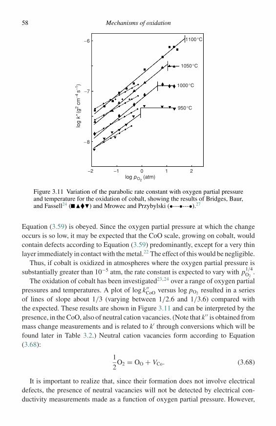
58 Mechanisms of oxidation
1100°C
1050°C
1000°C
950°C
−2
−8
−7
−6
−1 0 1 2log pO2
(atm)
log
k" (
g2 cm
−4 s
−1)
Figure 3.11 Variation of the parabolic rate constant with oxygen partial pressureand temperature for the oxidation of cobalt, showing the results of Bridges, Baur,and Fassell24 ( ���) and Mrowec and Przybylski (•---•---•).27
Equation (3.59) is obeyed. Since the oxygen partial pressure at which the changeoccurs is so low, it may be expected that the CoO scale, growing on cobalt, wouldcontain defects according to Equation (3.59) predominantly, except for a very thinlayer immediately in contact with the metal.22 The effect of this would be negligible.
Thus, if cobalt is oxidized in atmospheres where the oxygen partial pressure issubstantially greater than 10−5 atm, the rate constant is expected to vary with p1/4
O2.
The oxidation of cobalt has been investigated23,24 over a range of oxygen partialpressures and temperatures. A plot of log k ′′
CoO versus log pO2 resulted in a seriesof lines of slope about 1/3 (varying between 1/2.6 and 1/3.6) compared withthe expected. These results are shown in Figure 3.11 and can be interpreted by thepresence, in the CoO, also of neutral cation vacancies. (Note that k′′ is obtained frommass change measurements and is related to k′ through conversions which will befound later in Table 3.2.) Neutral cation vacancies form according to Equation(3.68):
1
2O2 = OO + VCo. (3.68)
It is important to realize that, since their formation does not involve electricaldefects, the presence of neutral vacancies will not be detected by electrical con-ductivity measurements made as a function of oxygen partial pressure. However,
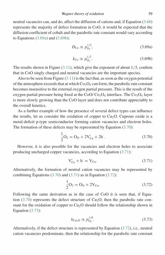
Wagner theory of oxidation 59
neutral vacancies can, and do, affect the diffusion of cations and, if Equation (3.68)represents the majority of defect formation in CoO, it would be expected that thediffusion coefficient of cobalt and the parabolic rate constant would vary accordingto Equations (3.69a) and (3.69b):
DCo ∝ p1/2O2
, (3.69a)
kCo ∝ p1/2O2
. (3.69b)
The results shown in Figure (3.11), which give the exponent of about 1/3, confirmthat in CoO singly charged and neutral vacancies are the important species.
Also to be seen from Figure (3.11) is the fact that, as soon as the oxygen potentialof the atmosphere exceeds that at which Co3O4 can form, the parabolic rate constantbecomes insensitive to the external oxygen partial pressure. This is the result of theoxygen partial pressure being fixed at the CoO/ Co3O4 interface. The Co3O4 layeris more slowly growing than the CoO layer and does not contribute appreciably tothe overall kinetics.
As a further example of how the presence of several defect types can influencethe results, let us consider the oxidation of copper to Cu2O. Cuprous oxide is ametal-deficit p-type semiconductor forming cation vacancies and electron holes.The formation of these defects may be represented by Equation (3.70):
1
2O2 = OO + 2V′
Cu + 2h·. (3.70)
However, it is also possible for the vacancies and electron holes to associateproducing uncharged copper vacancies, according to Equation (3.71):
V′Cu + h· = VCu. (3.71)
Alternatively, the formation of neutral cation vacancies may be represented bycombining Equations (3.70) and (3.71) as in Equation (3.72):
1
2O2 = OO + 2VCu. (3.72)
Following the same derivation as in the case of CoO it is seen that, if Equa-tion (3.70) represents the defect structure of Cu2O, then the parabolic rate con-stant for the oxidation of copper to Cu2O should follow the relationship shown inEquation (3.73):
kCu2O ∝ p1/8O2
. (3.73)
Alternatively, if the defect structure is represented by Equation (3.72), i.e., neutralcation vacancies predominate, then the relationship for the parabolic rate constant
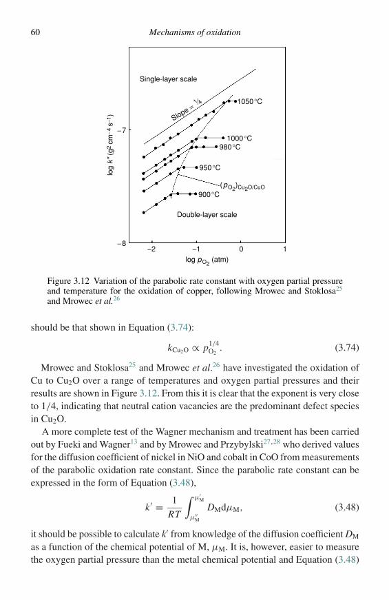
60 Mechanisms of oxidation
Single-layer scale
1050°C
1000°C980°C
950°C
log
k" (
g2 c
m−4
s−1
)
900°C
Double-layer scale
10−1−2−8
−7
(pO2)Cu2O/CuO
log pO2 (atm)
Slope =1 4
Figure 3.12 Variation of the parabolic rate constant with oxygen partial pressureand temperature for the oxidation of copper, following Mrowec and Stoklosa25
and Mrowec et al.26
should be that shown in Equation (3.74):
kCu2O ∝ p1/4O2
. (3.74)
Mrowec and Stoklosa25 and Mrowec et al.26 have investigated the oxidation ofCu to Cu2O over a range of temperatures and oxygen partial pressures and theirresults are shown in Figure 3.12. From this it is clear that the exponent is very closeto 1/4, indicating that neutral cation vacancies are the predominant defect speciesin Cu2O.
A more complete test of the Wagner mechanism and treatment has been carriedout by Fueki and Wagner13 and by Mrowec and Przybylski27,28 who derived valuesfor the diffusion coefficient of nickel in NiO and cobalt in CoO from measurementsof the parabolic oxidation rate constant. Since the parabolic rate constant can beexpressed in the form of Equation (3.48),
k ′ = 1
RT
∫ µ′M
µ′′M
DMdµM, (3.48)
it should be possible to calculate k′ from knowledge of the diffusion coefficient DM
as a function of the chemical potential of M, µM. It is, however, easier to measurethe oxygen partial pressure than the metal chemical potential and Equation (3.48)
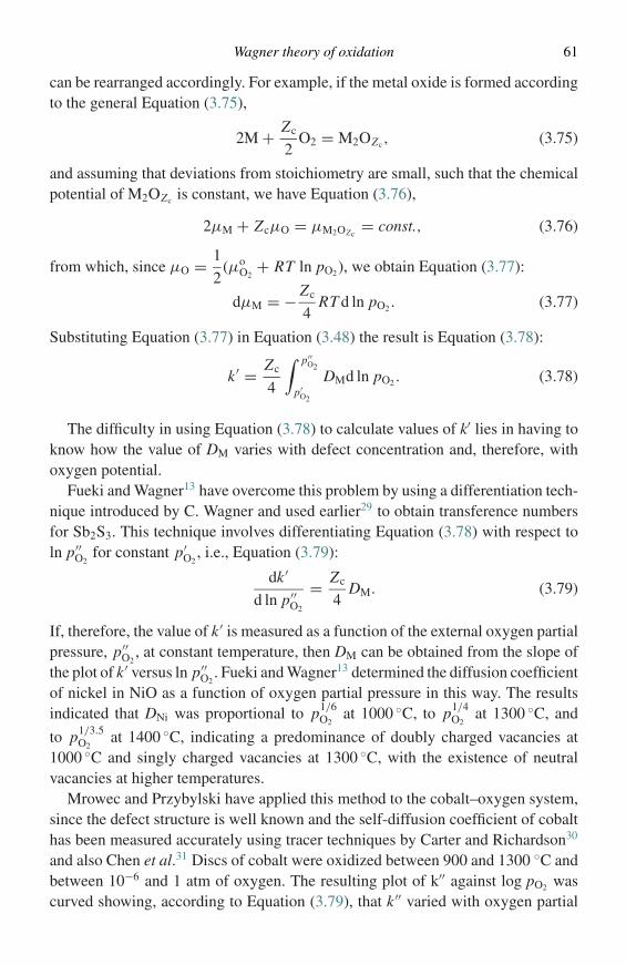
Wagner theory of oxidation 61
can be rearranged accordingly. For example, if the metal oxide is formed accordingto the general Equation (3.75),
2M + Zc
2O2 = M2OZc, (3.75)
and assuming that deviations from stoichiometry are small, such that the chemicalpotential of M2OZc is constant, we have Equation (3.76),
2µM + ZcµO = µM2OZc= const., (3.76)
from which, since µO = 1
2(µo
O2+ RT ln pO2), we obtain Equation (3.77):
dµM = − Zc
4RT d ln pO2 . (3.77)
Substituting Equation (3.77) in Equation (3.48) the result is Equation (3.78):
k ′ = Zc
4
∫ p′′O2
p′O2
DMd ln pO2 . (3.78)
The difficulty in using Equation (3.78) to calculate values of k′ lies in having toknow how the value of DM varies with defect concentration and, therefore, withoxygen potential.
Fueki and Wagner13 have overcome this problem by using a differentiation tech-nique introduced by C. Wagner and used earlier29 to obtain transference numbersfor Sb2S3. This technique involves differentiating Equation (3.78) with respect toln p′′
O2for constant p′
O2, i.e., Equation (3.79):
dk ′
d ln p′′O2
= Zc
4DM. (3.79)
If, therefore, the value of k ′ is measured as a function of the external oxygen partialpressure, p′′
O2, at constant temperature, then DM can be obtained from the slope of
the plot of k ′ versus ln p′′O2
. Fueki and Wagner13 determined the diffusion coefficientof nickel in NiO as a function of oxygen partial pressure in this way. The resultsindicated that DNi was proportional to p1/6
O2at 1000 ◦C, to p1/4
O2at 1300 ◦C, and
to p1/3.5O2
at 1400 ◦C, indicating a predominance of doubly charged vacancies at1000 ◦C and singly charged vacancies at 1300 ◦C, with the existence of neutralvacancies at higher temperatures.
Mrowec and Przybylski have applied this method to the cobalt–oxygen system,since the defect structure is well known and the self-diffusion coefficient of cobalthas been measured accurately using tracer techniques by Carter and Richardson30
and also Chen et al.31 Discs of cobalt were oxidized between 900 and 1300 ◦C andbetween 10−6 and 1 atm of oxygen. The resulting plot of k′′ against log pO2 wascurved showing, according to Equation (3.79), that k ′′ varied with oxygen partial
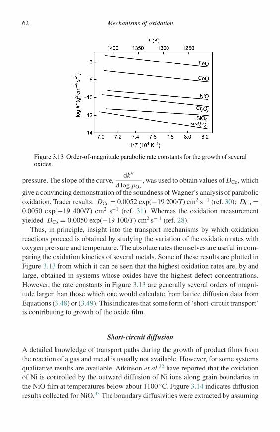
62 Mechanisms of oxidation
Figure 3.13 Order-of-magnitude parabolic rate constants for the growth of severaloxides.
pressure. The slope of the curve,dk ′′
d log pO2
, was used to obtain values of DCo, which
give a convincing demonstration of the soundness of Wagner’s analysis of parabolicoxidation. Tracer results: DCo = 0.0052 exp(−19 200/T) cm2 s−1 (ref. 30); DCo =0.0050 exp(−19 400/T) cm2 s−1 (ref. 31). Whereas the oxidation measurementyielded DCo = 0.0050 exp(−19 100/T) cm2 s− 1 (ref. 28).
Thus, in principle, insight into the transport mechanisms by which oxidationreactions proceed is obtained by studying the variation of the oxidation rates withoxygen pressure and temperature. The absolute rates themselves are useful in com-paring the oxidation kinetics of several metals. Some of these results are plotted inFigure 3.13 from which it can be seen that the highest oxidation rates are, by andlarge, obtained in systems whose oxides have the highest defect concentrations.However, the rate constants in Figure 3.13 are generally several orders of magni-tude larger than those which one would calculate from lattice diffusion data fromEquations (3.48) or (3.49). This indicates that some form of ‘short-circuit transport’is contributing to growth of the oxide film.
Short-circuit diffusion
A detailed knowledge of transport paths during the growth of product films fromthe reaction of a gas and metal is usually not available. However, for some systemsqualitative results are available. Atkinson et al.32 have reported that the oxidationof Ni is controlled by the outward diffusion of Ni ions along grain boundaries inthe NiO film at temperatures below about 1100 ◦C. Figure 3.14 indicates diffusionresults collected for NiO.33 The boundary diffusivities were extracted by assuming
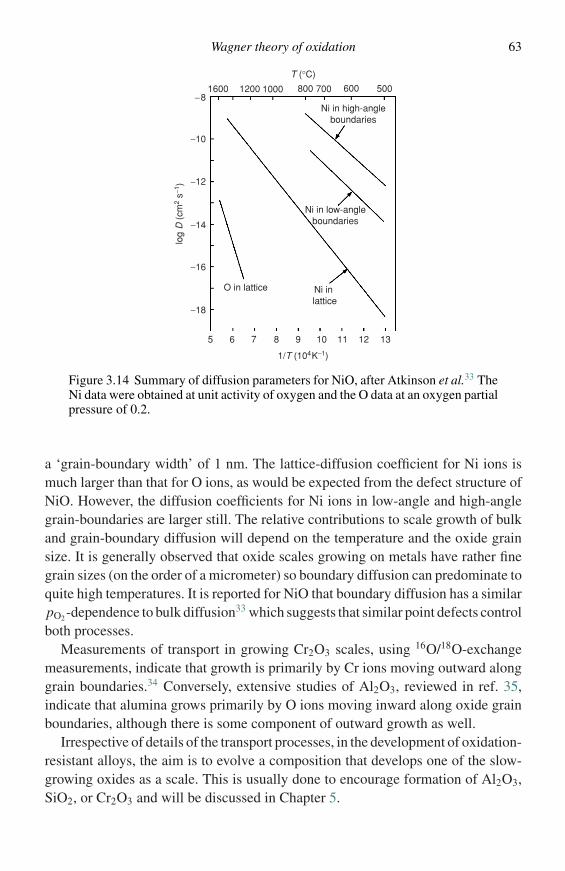
Wagner theory of oxidation 63
T (°C)
1600 1200 1000 800 700 600 500
Ni in high-angle boundaries
Ni in low-angle boundaries
Ni in lattice
O in lattice
log
D (
cm2
s−1)
1312111098
1/T (104K−1)
765
−18
−16
−12
−10
−8
−14
Figure 3.14 Summary of diffusion parameters for NiO, after Atkinson et al.33 TheNi data were obtained at unit activity of oxygen and the O data at an oxygen partialpressure of 0.2.
a ‘grain-boundary width’ of 1 nm. The lattice-diffusion coefficient for Ni ions ismuch larger than that for O ions, as would be expected from the defect structure ofNiO. However, the diffusion coefficients for Ni ions in low-angle and high-anglegrain-boundaries are larger still. The relative contributions to scale growth of bulkand grain-boundary diffusion will depend on the temperature and the oxide grainsize. It is generally observed that oxide scales growing on metals have rather finegrain sizes (on the order of a micrometer) so boundary diffusion can predominate toquite high temperatures. It is reported for NiO that boundary diffusion has a similarpO2-dependence to bulk diffusion33 which suggests that similar point defects controlboth processes.
Measurements of transport in growing Cr2O3 scales, using 16O/18O-exchangemeasurements, indicate that growth is primarily by Cr ions moving outward alonggrain boundaries.34 Conversely, extensive studies of Al2O3, reviewed in ref. 35,indicate that alumina grows primarily by O ions moving inward along oxide grainboundaries, although there is some component of outward growth as well.
Irrespective of details of the transport processes, in the development of oxidation-resistant alloys, the aim is to evolve a composition that develops one of the slow-growing oxides as a scale. This is usually done to encourage formation of Al2O3,SiO2, or Cr2O3 and will be discussed in Chapter 5.
64 Mechanisms of oxidation
Linear rate law
Under certain conditions the oxidation of a metal proceeds at a constant rate and issaid to obey the ‘linear rate law’, i.e., Equation (3.80),
x = klt, (3.80)
where x is the scale thickness and kl is the linear rate constant. The units of kl
depend upon the method used to follow the reaction. Where oxide scale thicknessis measured, as in Equation (3.80), then kl has the units cm s−1; if mass-gainmeasurement were to be used then the appropriate linear rate constant would haveunits of g cm−2 s−1, and so on.
The linear rate law is usually observed under conditions where a phase-boundaryprocess is the rate-determining step for the reaction, although other steps in themechanism of oxidation can lead to the same results. Principally, diffusion throughthe scale is unlikely to be rate limiting when the scale is thin, i.e., in the initialstages of the process. In this case, the metal–oxide and oxide–gas interfaces cannotbe assumed to be in thermodynamic equilibrium, although there are few knowncases where the reaction at the metal–scale interface has been found to play a rate-determining role. It can, therefore, be assumed that the reactions occurring at themetal–scale interface, i.e., the ionization of metal in the case of cation conductorsor ionization of metal and oxide formation in the case of anion conducting scales,are fast and, in general, attention can be turned to the process occurring at the scale–gas interface for an interpretation of the linear rate law.
At the scale–gas interface, the processes can be broken down into several steps.Reactant gas molecules must approach the scale surface and become adsorbedthere, the adsorbed molecules then split to form adsorbed oxygen, which eventuallyattracts electrons from the oxide lattice to become initially chemisorbed and finallyincorporated into the lattice. The removal of the electrons from the scale causesa change in the concentration of electron defects in the oxide at the scale–gasinterface. These processes can be represented as in Equation (3.81):
1
2O2(g) →
(1)
1
2O2(ad) →
(2)O(ad)
e−→(3)
O−(chem)e−→(4)
O2−(latt). (3.81)
which is written in terms of the oxygen molecule being the active oxidizing speciesin the gas phase. Except for cases of very low oxygen partial pressure, reactionscarried out in such atmospheres do not lead to constant rate kinetics. It can, there-fore, be assumed that the steps 1–4, which occur on the oxide surface, are fastreactions.
If, however, the oxidizing medium is a CO–CO2 mixture then constant rate kinet-ics are readily observed.36,37 In this case the surface reactions may be represented
Linear rate law 65
as in Equataion (3.82):
CO2(g) −→(1)
CO2(ad) −→(2)
CO(ad)↓
CO(g)
+CO(g)↓
O(ad)↓
CO2(g)
–e−→(3)
O−(chem) –e−→(4)
O2−(latt). (3.82)
Primarily, CO2 adsorbs onto the oxide surface and there dissociates to adsorbedCO and O species. The adsorbed oxygen then goes through the ionization stagesalready given in Equation (3.81). Two further processes are the desorption ofadsorbed carbon monoxide and the possibility of the removal of adsorbed oxy-gen by reaction with carbon monoxide molecules from the gas phase. Since steps3 and 4 can be assumed from above to be fast and since the rate of impingement ofCO2 on the scale surface, from atmospheres containing high concentrations of CO2,is high, the most likely rate-determining step is step 2 (dissociation of adsorbedcarbon dioxide to form adsorbed carbon monoxide molecules and oxygen atomson the surface of the oxide scale).
Hauffe and Pfeiffer36 investigated the oxidation of iron in CO–CO2 mixturesbetween 900 and 1000 ◦C and found that, under a total gas pressure of 1 atm, therate was constant and proportional to (pCO2/pCO)2/3, i.e, to p1/3
O2. They suggested
that this may indicate that chemisorption of oxygen is the rate-controlling step.The same reaction was investigated in more detail by Pettit et al.37 who assumed
that the rate-determining step was the dissociation of CO2 to give CO and adsorbedoxygen according to Equation (3.83):
CO2(g) = CO(g) + O(ad). (3.83)
If this assumption is correct, then the rate of the reaction per unit area n/A, wheren is the equivalents of oxide per unit time, would be given by Equation (3.84):
n
A= k ′ pCO2 − k ′′ pCO. (3.84)
where k ′ and k ′′ are constants specifying the rates of the forward and reverse reac-tions, respectively. During the initial stages of reaction, at least, the scale is largelyin equilibrium with the iron substrate, thus substantial changes in oxide-defectconcentrations at the scale–gas interface do not occur. Consequently, this factorplays no part in Equation (3.84).
If the gas had a composition in equilibrium with iron and wustite, then thereaction rate would be zero, i.e., n/A = 0. Consequently we would have Equation(3.85),
k ′′
k ′ = pCO2
pCO= K , (3.85)
66 Mechanisms of oxidation
where K is the equilibrium constant for the reaction Fe + CO2 = FeO + CO, and,therefore, from Equations (3.84) and (3.85), the rate under CO2/CO ratios exceedingthe equilibrium condition is given by Equation (3.86):
n
A= k ′(pCO2 − K pCO). (3.86)
The component partial pressures can be written in terms of the relevant mole frac-tions NCO2 and NCO and the total pressure P:
pCO2 = P NCO2, (3.87)
pCO = P NCO = P(1 − NCO2). (3.88)
Substituting Equations (3.87) and (3.88) in Equation (3.86) gives (Equation 3.89a),
n
A= k ′ P
[(1 + K ) NCO2 − K
], (3.89a)
which can be rearranged to Equation (3.89b),
n
A= k ′ P (1 + K )
[NCO2 − NCO2(eq)
], (3.89b)
where NCO2(eq) refers to the mole fraction of CO2 in the CO2/CO mixture inequilibrium with iron and wustite. According to Equation (3.89b) the oxidationrate at a given temperature should be proportional to both the mole fraction of CO2
in the gas and the total pressure of the gas.The experimental results for 925 ◦C shown in Figure 3.15 substantiate that both
of the above conditions are met and, therefore, the rate-determining step in thereaction is the decomposition of carbon dioxide to carbon monoxide and adsorbedoxygen.
Rarefied atmospheres
Constant reaction rates can also be observed during reactions of a metal underrarified atmospheres and with reactive gases diluted with an inert, non-reactive gas.
A good example of this case is the heat treatment of metals under partial vacuumwhen the atmosphere consists of nitrogen and oxygen molecules at a low pres-sure, where the rate-determining step is likely to be the rate of impingement ofoxygen molecules on the specimen surface. This rate can be calculated by usingthe Hertz–Knudsen–Langmuir equation derived from the kinetic theory of gases,Equation (3.90),
jO2 = αpO2(
2π MO2 RT)1/2 , (3.90)
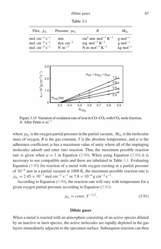
Dilute gases 67
Table 3.1
Flux, jO2 Pressure, pO2 R MO2
mol cm−2 s−1 atm cm3 atm mol−1 K−1 g mol−1
mol cm−2 s−1 dyn cm−2 erg mol−1 K−1 g mol−1
mol cm−2 s−1 N m−2 N m mol−1 K−1 kg mol−1
N co2
N co2(eq)
pco + pco2 = patm
kI ×
107 (
g cm
−2 s
−1)
0.3
1.0
0
2.0
3.0
0.4 0.5 0.6 0.7 0.8 0.9
0.4
0.6
0.8
1.0
Figure 3.15 Variation of oxidation rate of iron in CO–CO2 with CO2 mole fraction,N. After Pettit et al.37
where pO2 is the oxygen partial pressure in the partial vacuum, MO2 is the molecularmass of oxygen, R is the gas constant, T is the absolute temperature, and α is theadherence coefficient; α has a maximum value of unity where all of the impingingmolecules adsorb and enter into reaction. Thus the maximum possible reactionrate is given when α = 1 in Equation (3.90). When using Equation (3.90) it isnecessary to use compatible units and these are tabulated in Table 3.1. EvaluatingEquation (3.90) for reaction of a metal with oxygen existing at a partial pressureof 10−6 atm in a partial vacuum at 1000 K, the maximum possible reaction rate isjO2 = 2.45 × 10⁻⁷ mol cm−2 s−1 or 7.8 × 10⁻⁶ g cm−2 s−1.
According to Equation (3.90), the reaction rate will vary with temperature for agiven oxygen partial pressure according to Equation (3.91):
jO2 = const. T −1/2. (3.91)
Dilute gases
When a metal is reacted with an atmosphere consisting of an active species dilutedby an inactive or inert species, the active molecules are rapidly depleted in the gaslayers immediately adjacent to the specimen surface. Subsequent reaction can then
68 Mechanisms of oxidation
only proceed as long as molecules of the active species can diffuse through thedenuded layer to the metal surface. When the concentration of the active speciesis low in the atmosphere this step can become rate controlling. The denuded gaslayer next to the metal surface may be regarded as a boundary layer of thicknessδ. If the concentrations of the active species at the metal surface and in the bulkgas are expressed, respectively, by the partial pressure p′′
i and p′i then the rate at
which active species, i, diffuse across the boundary layer may be expressed as inEquation (3.92),
ji = −Dip′
i − p′′i
δ, (3.92)
which represents the maximum possible reaction rate observable under the circum-stances. In most cases, at least at the beginning of the reaction, the value of p′′
i isvery low and can be neglected giving Equation (3.93),
ji ≈ −Dip′
i
δ, (3.93)
i.e., the reaction rate is directly proportional to p′i , the partial pressure of the active
species in the bulk atmosphere. The sensitivity of the reaction rate to tempera-ture arises solely from the way in which Di and, to a lesser extent, δ varies withtemperature.
Reaction-rate control by this step can be identified most securely by the sensi-tivity of the reaction rate to the gas flow rate. If the gas flow rate is increased thethickness of the boundary layer is decreased and, correspondingly, the reaction rateincreases according to Equation (3.92).
It is important to note that the concentration of adsorbed species and, therefore,the rates of surface reactions involving adsorbed species also vary with the partialpressure of the active species in the gas phase. Thus, in order to identify boundary-layer transport as the process controlling a constant rate, the sensitivity of the rateto both active-species partial pressure and gas flow rate must be established.
Transition from linear law to parabolic law
It was stated earlier that constant-rate kinetics are often observed with thin scales.This is obviously a relative term and denotes the initial stages of a reaction whichmay continue for a long, or short, time depending on the conditions under whichthe reaction occurs.
Initially, when a scale is formed and is very thin, diffusion through the scale willbe rapid, establishing virtual equilibrium with the metal at the scale–gas interface.In other words, the metal activity at this interface will be maintained at a high value,initially close to unity, by rapid diffusion within the scale. Under these conditions,the rate of the reaction is likely to be controlled by one of the steps discussed above.
Logarithmic rate law 69
As the reaction proceeds at a constant rate the scale layer thickens, at the same timethe flux of ions through the scale must be equivalent to the surface reaction rate. Tomaintain this constant flux, the activity of the metal at the scale–gas interface mustfall as the scale thickens, eventually approaching the value in equilibrium with theatmosphere. Since the metal activity cannot fall below this value, further increasein scale thickness must result in a reduction in the metal activity gradient across thescale and, consequently, to a reduction in ionic flux and the reaction rate. At thispoint the transport of ions across the scale becomes the rate-controlling process andthe rate falls with time according to a parabolic rate law. The transition from linearto parabolic kinetics has been documented and described for the oxidation of ironin CO2–CO gas mixtures.38
Logarithmic rate law
When metals are oxidized under certain conditions, typically at low temperaturesof up to about 400 ◦C, the initial oxide formation, up to the 1000 Å range, ischaracterized by an initial rapid reaction that quickly reduces to a very low rateof reaction. Such behaviour has been found to conform to rate laws described bylogarithmic functions such as in Equations (3.94) and (3.95),
x = klog log (t + to) + A (direct log law), (3.94)
1/x = B − kil log t (inverse log law), (3.95)
where A, B, to, klog, and kil are constants at constant temperature.Several interpretations of this type of behaviour have been provided. For a
detailed description and summary, Kofstad39 and Hauffe40 should be consulted.Since the phenomenon is principally one that occurs at low temperatures, a strictlyqualitative description of the various interpretations will be given here, since thisphase of the oxidation reaction generally occurs during the heating period of aninvestigation into the formation of thick scales at high temperatures.
Interpretations of the logarithmic laws have been based on the adsorption of reac-tive species, the effects of electric fields developed across oxide layers, quantum-mechanical tunnelling of electrons through the thin scales, progressive blocking oflow-resistance diffusion paths, non-isothermal conditions in the oxide layer, andnucleation and growth processes. A concise summary of these theories has beengiven by Kofstad.39
Two things should be borne in mind. Firstly, it is difficult experimentally to obtainaccurate and reliable measurements of reaction rates relating to the formation of theinitial oxide layers, although, lately, modern high-vacuum techniques may allow anaccurate start to the reaction to be assumed by achieving thermal equilibrium beforeadmitting the reactant gas. Secondly, in any thermodynamic treatment carried out
70 Mechanisms of oxidation
to assess defect concentrations or concentration gradients, it may be necessary toinclude surface, or interfacial energies when considering such thin films. Thus,the actual deviations from stoichiometry in the film may be unknown. Similarlythe physical properties of the film may vary significantly from those of the bulkmaterial. Due to difficulties such as these, the interpretation of logarithmic ratebehaviour is the least-understood area of metal oxidation.
Adsorption has been assumed to be the rate-determining process during earlyoxide-film formation. When a clean surface is exposed to an oxidizing gas, eachmolecule impinging on the surface may either rebound or adsorb. The fraction, α,that remains adsorbed on the metal surface should be constant for a constant tem-perature and oxygen partial pressure. Therefore, under these conditions a constantreaction rate is expected. However, the value of α is markedly lower on those partsof the surface covered with a monolayer or oxide nuclei. Thus, as adsorption oroxide nucleation proceeds, the reaction rate is expected to decrease accordinglyuntil complete coverage of the surface by oxide has been achieved, when a muchlower rate is expected to be observed.
These initial processes of adsorption and nucleation have been investigated prin-cipally by Benard and coworkers,41 who have demonstrated convincingly that theinitial nucleation of oxide occurs at discrete sites on the metal surface. The oxideislands proceed to grow rapidly over the metal surface until complete coverage iseventually achieved. Furthermore, it has been demonstrated that the step of adsorp-tion begins at oxygen partial pressures significantly below the decomposition pres-sure of the oxide.
When the oxidizing gas chemisorbs onto the oxide surface growing on the metal,it captures, or withdraws, electrons from the oxide lattice according to Equation(3.81):
1
2O2(g) −→ O(ad)
e−−→ O−(chem). (3.81)
The result is to create additional electron holes in the surface of a p-type oxideor reduce the number of excess electrons in the surface of an n-type oxide. Theelectrons are withdrawn from a depth of about 100 Å over which, consequently, astrong electric field exists, known as a space charge. This concept has been usedby Cabrera and Mott42 to explain the inverse logarithmic law for the case of theformation of thin oxide films of very tight stoichiometry and, consequently, lowionic migration rates at low temperatures due to the low defect concentrations (theelectronic mobility is assumed to be greater than that of the ions). The electric fieldset up by chemisorption of oxygen, aided by quantum-mechanical tunneling ofelectrons from metal through the oxide to the adsorbed oxygen, acts on the mobile
Logarithmic rate law 71
ionic species and increases the migration rate. Clearly, since the potential differencebetween the metal and adsorbed oxygen species is assumed to be constant, thethinner the oxide layer the stronger the field and the faster the ionic diffusion. Asthe film thickens, the field strength is reduced and the reaction rate falls. When theoxide layer thickness exceeds about 100 Å, tunneling of electrons from the metalthrough the scale is not feasible and the full potential difference is no longer exerted.Thus, eventually, very low reaction rates are observed.
Inverse logarithmic rates have been reported by Young et al.43 for copper at70 ◦C, Hart44 for aluminium at 20 ◦C and Roberts45 for iron at temperatures up to120 ◦C.
Mott46 proposed an interpretation of the direct log law, later revised by Hauffe andIlschner,47 by explaining that the initial rapid reaction rates were due to quantum-mechanical tunneling of electrons through the thin oxide layer. Although electronsare not generally mobile in oxides at low temperatures, the electrical conductivityof thin oxide layers on metals is, surprisingly, much higher than would be expectedfrom bulk electrical properties. Thus, if the transport of electrons were the rate-determining step, the reaction rate would be surprisingly high in the initial stageswhen the film is very thin. As the film thickens, the maximum thickness for whichtunneling of electrons is valid is exceeded and the observed reaction rate falls awaymarkedly.
Other interpretations of log laws have rejected the assumption of uniform trans-port properties across the oxide layers and assume instead that paths for rapid ionictransport exist, e.g., along grain boundaries, or dislocation pipes, or over the sur-face of pores. These paths are progressively blocked as growth proceeds, eitherby recrystallization and grain growth, or by blocking of pores by growth stressesin the oxide, or by a combination of all three processes. It is also possible thatpores may act as vacancy sinks in the oxide and grow into cavities large enough tointerfere effectively with ionic transport by reducing the cross-section of compactoxide through which transport may occur. The formation of second-phase alloyoxides of low ionic conductivity may also give the same progressive resistanceto ionic migration. These theories have been considered primarily by Evans andco-workers.48
In view of the multiple interpretations available, it is clearly wise in practice toinvestigate thoroughly and judge each case on its merits rather than pass verdictfrom a simple examination of kinetics alone.
The presentation of Wagner’s treatment of high-temperature oxidation of metalsgiven here follows the original very closely. One of the assumptions made in thistreatment is that the oxide scale under consideration is thick compared with thedistance over which space-charge effects, discussed above, occur. Fromhold49–51
72 Mechanisms of oxidation
has considered the effect of the presence of space charges at the scale–gas andmetal–scale interfaces. His conclusions show that their presence would cause therate constant to vary with scale thickness in the range of 5000–10 000 Å. Thisanalysis is not considered further here since the oxide scales normally encounteredare very much thicker than this.
Relationships between parabolic rate constants
In the above treatment the parabolic rate constant is derived for the units relatingto measurement of the oxide thickness as the reaction parameter. As mentionedbefore, there are several methods of following the reaction depending on choiceof reaction parameters, each of which produces its own particular parabolic rateconstant, as shown below using Wagner’s notation for the various parabolic rateconstants.
(a) Measurement of scale thickness (x):
dx
dt= k ′
x, i.e., x2 = 2k ′t. (3.25)
In Equation (3.25) k ′ is the ‘practical tarnishing constant’ or ‘scaling constant’ and hasunits of cm2 s−1.
(b) Measurement of the mass increase of the specimen (m)The parabolic rate constant k ′′ is defined by Equation (3.96),(m
A
)2= k ′′t, (3.96)
where A is the area over which reaction occurs; k ′′ is also referred to as the practicaltarnishing constant or ‘scaling constant’ and has units of g2 cm−4 s−1.
(c) Measurement of metal surface recession (l)Measuring the thickness of metal consumed leads to the relationship defining kc, Equa-tion (3.97); kc is called the ‘corrosion constant’ and has units of cm2 s−1:
l2 = 2kct. (3.97)
(d) Rate of growth of scale of unit thicknessThe rational rate constant is defined as the rate of growth over unit area, in equivalentsper second, of a scale of unit thickness, i.e., Equation (3.98),
kr = x
A
dn
dt, (3.98)
where n is the number of equivalents in the oxide layer of thickness x.kr is sometimes called the theoretical tarnishing constant and has units of equivalentscm−1 s−1.
It is easy to see that having so many different ways of expressing parabolic rateconstants, and so many different symbols, produces a situation ripe for confusion.
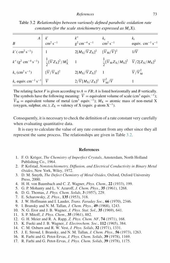
References 73
Table 3.2 Relationships between variously defined parabolic oxidation rateconstants (for the scale stoichiometry expressed as MνX).
A k′ k′′ kc kr
B cm2 s−1 g2 cm−4 s−1 cm2 s−1 equiv. cm−1 s−1
k ′ ( cm2 s−1) 1 2[MX/V ZX]2 [V M/V ]2 1/V
k ′′ (g2 cm−4 s−1)1
2[V ZX]2/M2
X 11
2[V M ZX/MX]2 V /2[ZX/MX]2
kc (cm2 s−1) [V /V M]2 2[MX/V ZX]2 1 V /V2M
kr equiv. cm−1 s−1 V 2/V [MX/ZX]2 V2M/V 1
The relating factor F is given according to A = FB; A is listed horizontally and B vertically.The symbols have the following meaning: V = equivalent volume of scale (cm3 equiv.−1);V M = equivalent volume of metal (cm3 equiv.−1); MX = atomic mass of non-metal X(oxygen, sulphur, etc.); ZX = valency of X (equiv. g-atom X−1).
Consequently, it is necessary to check the definition of a rate constant very carefullywhen evaluating quantitative data.
It is easy to calculate the value of any rate constant from any other since they allrepresent the same process. The relationships are given in Table 3.2.
References
1. F. O. Kroger, The Chemistry of Imperfect Crystals, Amsterdam, North HollandPublishing Co., 1964.
2. P. Kofstad, Nonstoichiometry, Diffusion, and Electrical Conductivity in Binary MetalOxides, New York, Wiley, 1972.
3. D. M. Smyth, The Defect Chemistry of Metal Oxides, Oxford, Oxford UniversityPress, 2000.
4. H. H. von Baumbach and C. Z. Wagner, Phys. Chem., 22 (1933), 199.5. G. P. Mohanty and L. V. Azaroff, J. Chem. Phys., 35 (1961), 1268.6. D. G. Thomas, J. Phys. Chem. Solids, 3 (1957), 229.7. E. Scharowsky, Z. Phys., 135 (1953), 318.8. J. W. Hoffmann and I. Lauder, Trans. Faraday Soc., 66 (1970), 2346.9. I. Bransky and N. M. Tallan, J. Chem. Phys., 49 (1968), 1243.
10. N. G. Eror and J. B. Wagner, J. Phys. Stat. Sol., 35 (1969), 641.11. S. P. Mitoff, J. Phys. Chem., 35 (1961), 882.12. G. H. Meier and R. A. Rapp, Z. Phys. Chem. NF, 74 (1971), 168.13. K. Fueki and J. B. Wagner, J. Electrochem. Soc., 112 (1965), 384.14. C. M. Osburn and R. W. Vest, J. Phys. Solids, 32 (1971), 1331.15. J. E. Stroud, I. Bransky, and N. M. Tallan, J. Chem. Phys., 56 (1973), 1263.16. R. Farhi and G. Petot-Ervas, J. Phys. Chem. Solids, 39 (1978), 1169.17. R. Farhi and G. Petot-Ervas, J. Phys. Chem. Solids, 39 (1978), 1175.
74 Mechanisms of oxidation
18. G. J. Koel and P. J. Gellings, Oxid. Met., 5 (1972), 185.19. M. C. Pope and N. Birks, Corr. Sci., 17 (1977), 747.20. C. Wagner, Z. Phys. Chem., 21 (1933), 25.21. B. Fisher and D. S. Tannhauser, J. Chem. Phys., 44 (1966), 1663.22. N. G. Eror and J. B. Wagner, J. Phys. Chem. Solids, 29 (1968), 1597.23. R. E. Carter and F. D. Richardson, TAIME, 203 (1955), 336.24. D. W. Bridges, J. P. Baur, and W. M. Fassell, J. Electrochem. Soc., 103 (1956), 619.25. S. Mrowec and A. Stoklosa, Oxid. Met., 3 (1971), 291.26. S. Mrowec, A. Stoklosa, and K. Godlewski, Cryst. Latt. Def., 5 (1974), 239.27. S. Mrowec and K. Przybylski, Oxid. Met., 11 (1977), 365.28. S. Mrowec and K. Przybylski, Oxid. Met., 11 (1977), 383.29. F. S. Pettit, J. Phys. Chem., 68 (1964), 9.30. R. E. Carter and F. D. Richardson,, J. Met., 6 (1954), 1244.31. W. K. Chen, N. L. Peterson, and W. T., Reeves, Phys. Rev., 186 (1969),
887.32. A. Atkinson, R. I. Taylor, and A. E. Hughes, Phil. Mag., A45 (1982), 823.33. A. Atkinson, D. P. Moon, D. W. Smart, and R. I. Taylor, J. Mater. Sci., 21 (1986),
1747.34. R. J. Hussey and M. J. Graham, Oxid. Met., 45 (1996), 349.35. R. Prescott and M. J. Graham, Oxid. Met., 38 (1992), 233.36. K. Hauffe and H. Pfeiffer, Z. Elektrochem., 56 (1952), 390.37. F. S. Pettit, R. Yinger, and J. B. Wagner, Acta Met., 8 (1960), 617.38. F. S. Pettit and J. B. Wagner, Acta Met., 12 (1964), 35.39. P. Kofstad, High Temperature Corrosion, New York, Elsevier Applied Science
Publishers, Ltd, 1988.40. K. Hauffe, Oxidation of Metals, New York, Plenum Press, 1965.41. J. Benard, Oxydation des Meteaux, Paris, Gautier-Villars, 1962.42. N. Cabrera and N. F. Mott, Rept. Prog. Phys., 12 (1948), 163.43. F. W. Young, J. V. Cathcart, and A. T. Gwathmey, Acta Met., 4 (1956), 145.44. R. K. Hart, Proc. Roy. Soc., 236A (1956), 68.45. M. W. Roberts, Trans. Faraday Soc., 57 (1961), 99.46. N. F. Mott, Trans. Faraday Soc., 36 (1940), 472.47. K. Hauffe and B. Z. Ilschner, Elektrochem., 58 (1954), 382.48. U. R. Evans, The Corrosion and Oxidation of Metals, London, Edward Arnold, 1960.49. A. T. Fromhold, J. Phys. Chem. Solids, 33 (1972), 95.50. A. T. Fromhold and E. L. Cook, J. Phys. Chem. Solids, 33 (1972), 95.51. A. T. Fromhold, J. Phys. Soc. J., 48 (1980), 2022.
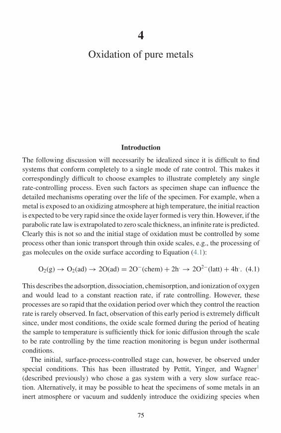
4
Oxidation of pure metals
Introduction
The following discussion will necessarily be idealized since it is difficult to findsystems that conform completely to a single mode of rate control. This makes itcorrespondingly difficult to choose examples to illustrate completely any singlerate-controlling process. Even such factors as specimen shape can influence thedetailed mechanisms operating over the life of the specimen. For example, when ametal is exposed to an oxidizing atmosphere at high temperature, the initial reactionis expected to be very rapid since the oxide layer formed is very thin. However, if theparabolic rate law is extrapolated to zero scale thickness, an infinite rate is predicted.Clearly this is not so and the initial stage of oxidation must be controlled by someprocess other than ionic transport through thin oxide scales, e.g., the processing ofgas molecules on the oxide surface according to Equation (4.1):
O2(g) → O2(ad) → 2O(ad) = 2O−(chem) + 2h. → 2O2−(latt) + 4h.. (4.1)
This describes the adsorption, dissociation, chemisorption, and ionization of oxygenand would lead to a constant reaction rate, if rate controlling. However, theseprocesses are so rapid that the oxidation period over which they control the reactionrate is rarely observed. In fact, observation of this early period is extremely difficultsince, under most conditions, the oxide scale formed during the period of heatingthe sample to temperature is sufficiently thick for ionic diffusion through the scaleto be rate controlling by the time reaction monitoring is begun under isothermalconditions.
The initial, surface-process-controlled stage can, however, be observed underspecial conditions. This has been illustrated by Pettit, Yinger, and Wagner1
(described previously) who chose a gas system with a very slow surface reac-tion. Alternatively, it may be possible to heat the specimens of some metals in aninert atmosphere or vacuum and suddenly introduce the oxidizing species when
75
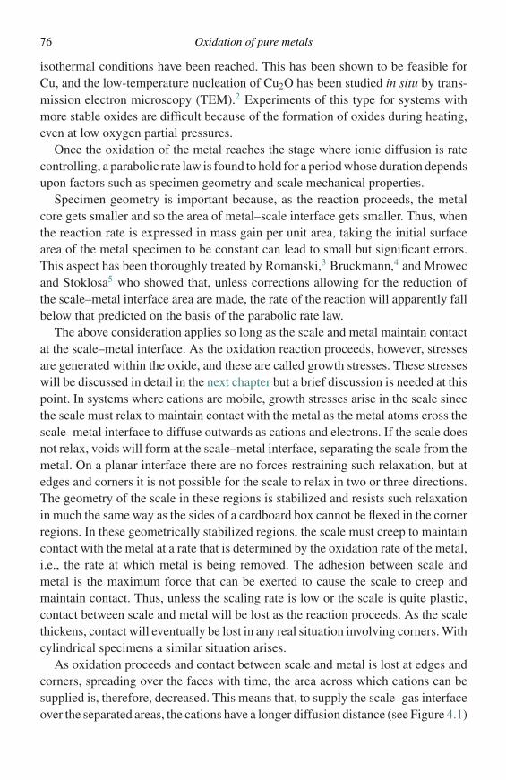
76 Oxidation of pure metals
isothermal conditions have been reached. This has been shown to be feasible forCu, and the low-temperature nucleation of Cu2O has been studied in situ by trans-mission electron microscopy (TEM).2 Experiments of this type for systems withmore stable oxides are difficult because of the formation of oxides during heating,even at low oxygen partial pressures.
Once the oxidation of the metal reaches the stage where ionic diffusion is ratecontrolling, a parabolic rate law is found to hold for a period whose duration dependsupon factors such as specimen geometry and scale mechanical properties.
Specimen geometry is important because, as the reaction proceeds, the metalcore gets smaller and so the area of metal–scale interface gets smaller. Thus, whenthe reaction rate is expressed in mass gain per unit area, taking the initial surfacearea of the metal specimen to be constant can lead to small but significant errors.This aspect has been thoroughly treated by Romanski,3 Bruckmann,4 and Mrowecand Stoklosa5 who showed that, unless corrections allowing for the reduction ofthe scale–metal interface area are made, the rate of the reaction will apparently fallbelow that predicted on the basis of the parabolic rate law.
The above consideration applies so long as the scale and metal maintain contactat the scale–metal interface. As the oxidation reaction proceeds, however, stressesare generated within the oxide, and these are called growth stresses. These stresseswill be discussed in detail in the next chapter but a brief discussion is needed at thispoint. In systems where cations are mobile, growth stresses arise in the scale sincethe scale must relax to maintain contact with the metal as the metal atoms cross thescale–metal interface to diffuse outwards as cations and electrons. If the scale doesnot relax, voids will form at the scale–metal interface, separating the scale from themetal. On a planar interface there are no forces restraining such relaxation, but atedges and corners it is not possible for the scale to relax in two or three directions.The geometry of the scale in these regions is stabilized and resists such relaxationin much the same way as the sides of a cardboard box cannot be flexed in the cornerregions. In these geometrically stabilized regions, the scale must creep to maintaincontact with the metal at a rate that is determined by the oxidation rate of the metal,i.e., the rate at which metal is being removed. The adhesion between scale andmetal is the maximum force that can be exerted to cause the scale to creep andmaintain contact. Thus, unless the scaling rate is low or the scale is quite plastic,contact between scale and metal will be lost as the reaction proceeds. As the scalethickens, contact will eventually be lost in any real situation involving corners. Withcylindrical specimens a similar situation arises.
As oxidation proceeds and contact between scale and metal is lost at edges andcorners, spreading over the faces with time, the area across which cations can besupplied is, therefore, decreased. This means that, to supply the scale–gas interfaceover the separated areas, the cations have a longer diffusion distance (see Figure 4.1)
Introduction 77
2+
Figure 4.1 Schematic diagram showing longer diffusion distance for cationsto supply scale–gas interface when scale–metal separation occurs at edges andcorners.
Grain boundary
Compactscale
Porousscale
Gas
Metal
O2 O2 O2
O2 O2
M2+
e−M2+
e−
M2+
e−M2+
e−
M2+
e−
M2+
e−M2+
e−M2+
e−M2+
e− M2+
e−
Figure 4.2 Mechanism of formation of porous zone resulting from scale–metalseparation. Note that the scale decomposes more readily at the grain boundariesin the scale than at the grain surfaces.
and hence the reaction rate falls, unless vaporization of the metal across the voidcan keep up with the oxide growth. This leads to specific reaction rates that arelower than expected when the original metal surface area is used in the calculation.
Frequently this loss of contact causes the formation of a porous zone of scalebetween the outer compact layer and the metal. The mechanism of formation is quitestraightforward, as outlined below and shown in Figure 4.2. When scale separationoccurs, the metal activity at the inner surface of the scale is high and so cationsstill continue to migrate outwards. However, this causes the metal activity to falland the oxygen activity to rise correspondingly. As the oxygen activity rises, theoxygen partial pressure in local equilibrium with the scale inner surface rises andoxygen ‘evaporates’ into the pore, diffuses across the pore, and forms oxide on themetal surface. In this way a porous layer can be formed next to the scale–metal
78 Oxidation of pure metals
interface while maintaining outward cation diffusion. The oxide scale dissociatesmore rapidly at grain boundaries than at grain surfaces.
The above discussion shows that physical aspects of the scale and scale–metalinterface configuration can markedly influence the apparent kinetic behaviour andrate appearance. It cannot be emphasized too strongly that careful metallographicand other examination is essential for accurate and correct interpretation of observedkinetics. These factors also indicate that specimen size may influence the course ofthe kinetics. Thus, extrapolating from results on small specimens to predict resultson large pieces or pieces of different geometry may not be easy or feasible. Theabove and other aspects will be brought out in the following discussion of theoxidation of selected pure metals.
Systems forming single-layer scales
Oxidation of nickel
Nickel is an ideal metal for oxidation studies since, under normal temperature andpressure conditions, it forms only one oxide, NiO, which is a p-type semiconductorwith cation deficit. The mechanism by which oxidation of nickel proceeds is, there-fore, expected simply to involve the outward migration of cations and electronsforming a single-phase scale.
Early measurements of the oxidation of nickel over the temperature range 700–1300 ◦C showed a surprising variation of the parabolic rate constant over fourorders of magnitude.6–8 Later determinations, using nickel of significantly improvedpurity,9,10 showed that the parabolic rate constant for nickel containing 0.002%impurity was reliably reproducible and was lower than that for the less-pure nickelsamples used earlier. Since the majority of impurity elements found in nickel areeither divalent or trivalent, they will, when dissolved in the oxide, either have noeffect on or increase the mobility of cations in NiO. It is, therefore, understandablethat the impure nickel specimens were found in general to oxidize more rapidly thanpure nickel. The activation energy of the process remained fairly constant regardlessof impurity level indicating that the rate-determining step remained unchanged. Thescale morphology has also been found to vary significantly with the purity of themetal. This is particularly well demonstrated by results obtained at 1000 ◦C.11
Using nickel of high purity a compact, adherent, single-layer scale of NiO isformed. Platinum markers, placed on the metal surface before reaction, are foundafterwards at the scale–metal interface. This is very strong evidence that the scaleforms entirely by the outward migration of cations and electrons.
Earlier work using nickel that contained low concentrations of impurities (0.1%)showed that a fundamentally different scale was produced. In this case the scaleconsisted of two layers, both of NiO, the outer compact and the inner porous.
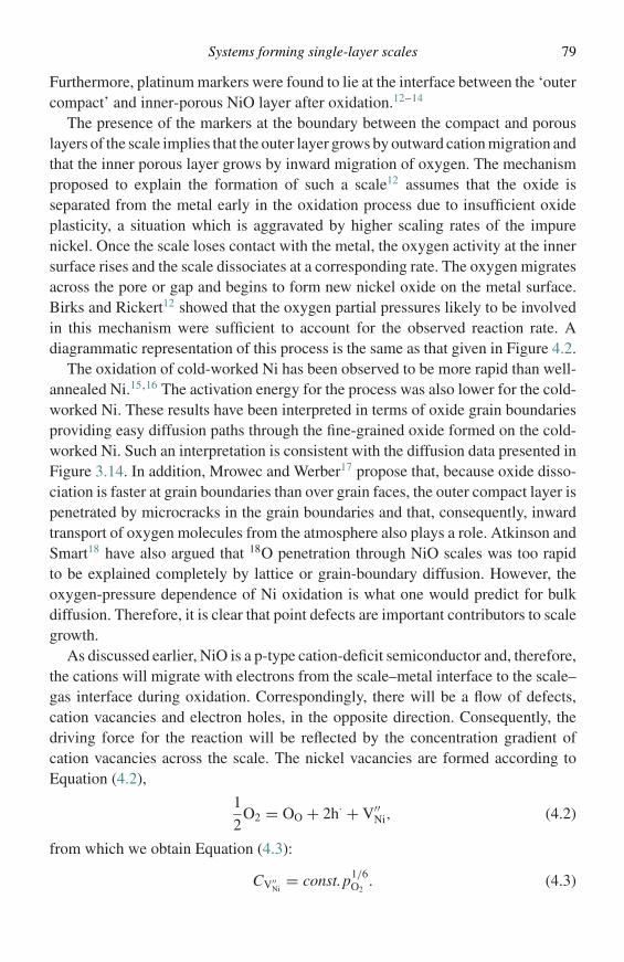
Systems forming single-layer scales 79
Furthermore, platinum markers were found to lie at the interface between the ‘outercompact’ and inner-porous NiO layer after oxidation.12–14
The presence of the markers at the boundary between the compact and porouslayers of the scale implies that the outer layer grows by outward cation migration andthat the inner porous layer grows by inward migration of oxygen. The mechanismproposed to explain the formation of such a scale12 assumes that the oxide isseparated from the metal early in the oxidation process due to insufficient oxideplasticity, a situation which is aggravated by higher scaling rates of the impurenickel. Once the scale loses contact with the metal, the oxygen activity at the innersurface rises and the scale dissociates at a corresponding rate. The oxygen migratesacross the pore or gap and begins to form new nickel oxide on the metal surface.Birks and Rickert12 showed that the oxygen partial pressures likely to be involvedin this mechanism were sufficient to account for the observed reaction rate. Adiagrammatic representation of this process is the same as that given in Figure 4.2.
The oxidation of cold-worked Ni has been observed to be more rapid than well-annealed Ni.15,16 The activation energy for the process was also lower for the cold-worked Ni. These results have been interpreted in terms of oxide grain boundariesproviding easy diffusion paths through the fine-grained oxide formed on the cold-worked Ni. Such an interpretation is consistent with the diffusion data presented inFigure 3.14. In addition, Mrowec and Werber17 propose that, because oxide disso-ciation is faster at grain boundaries than over grain faces, the outer compact layer ispenetrated by microcracks in the grain boundaries and that, consequently, inwardtransport of oxygen molecules from the atmosphere also plays a role. Atkinson andSmart18 have also argued that 18O penetration through NiO scales was too rapidto be explained completely by lattice or grain-boundary diffusion. However, theoxygen-pressure dependence of Ni oxidation is what one would predict for bulkdiffusion. Therefore, it is clear that point defects are important contributors to scalegrowth.
As discussed earlier, NiO is a p-type cation-deficit semiconductor and, therefore,the cations will migrate with electrons from the scale–metal interface to the scale–gas interface during oxidation. Correspondingly, there will be a flow of defects,cation vacancies and electron holes, in the opposite direction. Consequently, thedriving force for the reaction will be reflected by the concentration gradient ofcation vacancies across the scale. The nickel vacancies are formed according toEquation (4.2),
1
2O2 = OO + 2h· + V′′
Ni, (4.2)
from which we obtain Equation (4.3):
CV′′Ni
= const.p1/6O2
. (4.3)
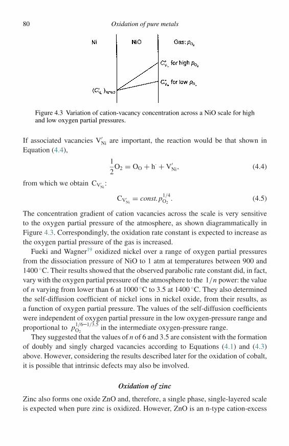
80 Oxidation of pure metals
Figure 4.3 Variation of cation-vacancy concentration across a NiO scale for highand low oxygen partial pressures.
If associated vacancies V′Ni are important, the reaction would be that shown in
Equation (4.4),
1
2O2 = OO + h· + V′
Ni, (4.4)
from which we obtain CV′Ni
:
CV′Ni
= const.p1/4O2
. (4.5)
The concentration gradient of cation vacancies across the scale is very sensitiveto the oxygen partial pressure of the atmosphere, as shown diagrammatically inFigure 4.3. Correspondingly, the oxidation rate constant is expected to increase asthe oxygen partial pressure of the gas is increased.
Fueki and Wagner19 oxidized nickel over a range of oxygen partial pressuresfrom the dissociation pressure of NiO to 1 atm at temperatures between 900 and1400 ◦C. Their results showed that the observed parabolic rate constant did, in fact,vary with the oxygen partial pressure of the atmosphere to the 1/n power: the valueof n varying from lower than 6 at 1000 ◦C to 3.5 at 1400 ◦C. They also determinedthe self-diffusion coefficient of nickel ions in nickel oxide, from their results, asa function of oxygen partial pressure. The values of the self-diffusion coefficientswere independent of oxygen partial pressure in the low oxygen-pressure range andproportional to p1/6–1/3.5
O2in the intermediate oxygen-pressure range.
They suggested that the values of n of 6 and 3.5 are consistent with the formationof doubly and singly charged vacancies according to Equations (4.1) and (4.3)above. However, considering the results described later for the oxidation of cobalt,it is possible that intrinsic defects may also be involved.
Oxidation of zinc
Zinc also forms one oxide ZnO and, therefore, a single phase, single-layered scaleis expected when pure zinc is oxidized. However, ZnO is an n-type cation-excess
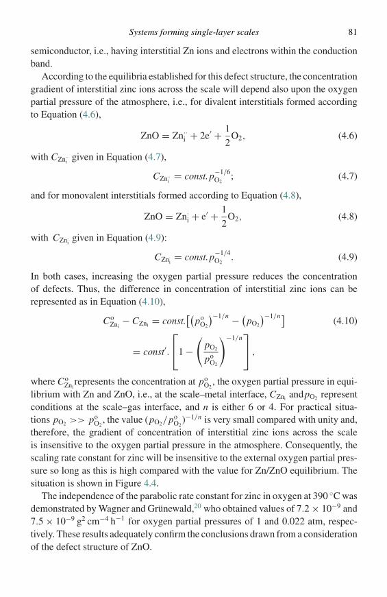
Systems forming single-layer scales 81
semiconductor, i.e., having interstitial Zn ions and electrons within the conductionband.
According to the equilibria established for this defect structure, the concentrationgradient of interstitial zinc ions across the scale will depend also upon the oxygenpartial pressure of the atmosphere, i.e., for divalent interstitials formed accordingto Equation (4.6),
ZnO = Zn··i + 2e′ + 1
2O2, (4.6)
with CZn··i
given in Equation (4.7),
CZn··i= const.p−1/6
O2; (4.7)
and for monovalent interstitials formed according to Equation (4.8),
ZnO = Zn·i + e′ + 1
2O2, (4.8)
with CZn·igiven in Equation (4.9):
CZn·i= const.p−1/4
O2. (4.9)
In both cases, increasing the oxygen partial pressure reduces the concentrationof defects. Thus, the difference in concentration of interstitial zinc ions can berepresented as in Equation (4.10),
CoZni
− CZni = const.[(
poO2
)−1/n − (pO2
)−1/n](4.10)
= const′.
1 −
(pO2
poO2
)−1/n ,
where CoZni
represents the concentration at poO2
, the oxygen partial pressure in equi-librium with Zn and ZnO, i.e., at the scale–metal interface, CZni andpO2 representconditions at the scale–gas interface, and n is either 6 or 4. For practical situa-tions pO2 >> po
O2, the value (pO2/po
O2)−1/n is very small compared with unity and,
therefore, the gradient of concentration of interstitial zinc ions across the scaleis insensitive to the oxygen partial pressure in the atmosphere. Consequently, thescaling rate constant for zinc will be insensitive to the external oxygen partial pres-sure so long as this is high compared with the value for Zn/ZnO equilibrium. Thesituation is shown in Figure 4.4.
The independence of the parabolic rate constant for zinc in oxygen at 390 ◦C wasdemonstrated by Wagner and Grunewald,20 who obtained values of 7.2 × 10⁻⁹ and7.5 × 10−9 g2 cm−4 h−1 for oxygen partial pressures of 1 and 0.022 atm, respec-tively. These results adequately confirm the conclusions drawn from a considerationof the defect structure of ZnO.
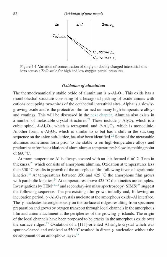
82 Oxidation of pure metals
Figure 4.4 Variation of concentration of singly or doubly charged interstitial zincions across a ZnO scale for high and low oxygen partial pressures.
Oxidation of aluminium
The thermodynamically stable oxide of aluminium is α-Al2O3. This oxide has arhombohedral structure consisting of a hexagonal packing of oxide anions withcations occupying two-thirds of the octahedral interstitial sites. Alpha is a slowly-growing oxide and is the protective film formed on many high-temperature alloysand coatings. This will be discussed in the next chapter. Alumina also exists ina number of metastable crystal structures.21 These include γ -Al2O3, which is acubic spinel, δ-Al2O3, which is tetragonal, and θ -Al2O3, which is monoclinic.Another form, κ-Al2O3, which is similar to α but has a shift in the stackingsequence on the anion sub-lattice, has also been identified.22 Some of the metastablealuminas sometimes form prior to the stable α on high-temperature alloys andpredominate for the oxidation of aluminium at temperatures below its melting pointof 660 ◦C.
At room temperature Al is always covered with an ‘air-formed film’ 2–3 nm inthickness,23 which consists of amorphous alumina. Oxidation at temperatures lessthan 350 ◦C results in growth of the amorphous film following inverse logarithmickinetics.24 At temperatures between 350 and 425 ◦C the amorphous film growswith parabolic kinetics.24 At temperatures above 425 ◦C the kinetics are complex.Investigations by TEM23,24 and secondary-ion mass spectroscopy (SIMS)25 suggestthe following sequence. The pre-existing film grows initially and, following anincubation period, γ -Al2O3 crystals nucleate at the amorphous oxide–Al interface.The γ nucleates heterogeneously on the surface at ridges resulting from specimenpreparation and grows by oxygen transport through local channels in the amorphousfilm and anion attachment at the peripheries of the growing γ islands. The originof the local channels have been proposed to be cracks in the amorphous oxide overthe surface ridges.23 Oxidation of a [111]-oriented Al single crystal which wassputter-cleaned and oxidized at 550 ◦C resulted in direct γ nucleation without thedevelopment of an amorphous layer.25
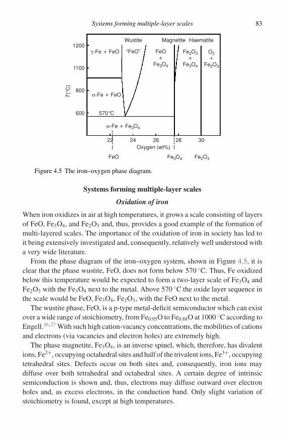
Systems forming multiple-layer scales 83
1200
1100
800
600
α-Fe + FeO
α-Fe + Fe3O4
Fe3O4FeO Fe2O3
570 °C
T(°
C)
2422 26Oxygen (wt%)
Wustite Magnetite Haematite
28 30
γ -Fe + FeO “FeO” FeO+
Fe3O4
Fe2O3+
Fe3O4
O2+
Fe2O3
Figure 4.5 The iron–oxygen phase diagram.
Systems forming multiple-layer scales
Oxidation of iron
When iron oxidizes in air at high temperatures, it grows a scale consisting of layersof FeO, Fe3O4, and Fe2O3 and, thus, provides a good example of the formation ofmulti-layered scales. The importance of the oxidation of iron in society has led toit being extensively investigated and, consequently, relatively well understood witha very wide literature.
From the phase diagram of the iron–oxygen system, shown in Figure 4.5, it isclear that the phase wustite, FeO, does not form below 570 ◦C. Thus, Fe oxidizedbelow this temperature would be expected to form a two-layer scale of Fe3O4 andFe2O3 with the Fe3O4 next to the metal. Above 570 ◦C the oxide layer sequence inthe scale would be FeO, Fe3O4, Fe2O3, with the FeO next to the metal.
The wustite phase, FeO, is a p-type metal-deficit semiconductor which can existover a wide range of stoichiometry, from Fe0.95O to Fe0.88O at 1000 ◦C according toEngell.26,27 With such high cation-vacancy concentrations, the mobilities of cationsand electrons (via vacancies and electron holes) are extremely high.
The phase magnetite, Fe3O4, is an inverse spinel, which, therefore, has divalentions, Fe2+, occupying octahedral sites and half of the trivalent ions, Fe3+, occupyingtetrahedral sites. Defects occur on both sites and, consequently, iron ions maydiffuse over both tetrahedral and octahedral sites. A certain degree of intrinsicsemiconduction is shown and, thus, electrons may diffuse outward over electronholes and, as excess electrons, in the conduction band. Only slight variation ofstoichiometry is found, except at high temperatures.
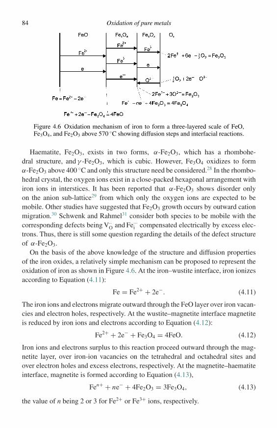
84 Oxidation of pure metals
Figure 4.6 Oxidation mechanism of iron to form a three-layered scale of FeO,Fe3O4, and Fe2O3 above 570 ◦C showing diffusion steps and interfacial reactions.
Haematite, Fe2O3, exists in two forms, α-Fe2O3, which has a rhombohe-dral structure, and γ -Fe2O3, which is cubic. However, Fe3O4 oxidizes to formα-Fe2O3 above 400 ◦C and only this structure need be considered.28 In the rhombo-hedral crystal, the oxygen ions exist in a close-packed hexagonal arrangement withiron ions in interstices. It has been reported that α-Fe2O3 shows disorder onlyon the anion sub-lattice29 from which only the oxygen ions are expected to bemobile. Other studies have suggested that Fe2O3 growth occurs by outward cationmigration.30 Schwenk and Rahmel31 consider both species to be mobile with thecorresponding defects being V··
O and Fe···i compensated electrically by excess elec-
trons. Thus, there is still some question regarding the details of the defect structureof α-Fe2O3.
On the basis of the above knowledge of the structure and diffusion propertiesof the iron oxides, a relatively simple mechanism can be proposed to represent theoxidation of iron as shown in Figure 4.6. At the iron–wustite interface, iron ionizesaccording to Equation (4.11):
Fe = Fe2+ + 2e−. (4.11)
The iron ions and electrons migrate outward through the FeO layer over iron vacan-cies and electron holes, respectively. At the wustite–magnetite interface magnetiteis reduced by iron ions and electrons according to Equation (4.12):
Fe2+ + 2e− + Fe3O4 = 4FeO. (4.12)
Iron ions and electrons surplus to this reaction proceed outward through the mag-netite layer, over iron-ion vacancies on the tetrahedral and octahedral sites andover electron holes and excess electrons, respectively. At the magnetite–haematiteinterface, magnetite is formed according to Equation (4.13),
Fen+ + ne− + 4Fe2O3 = 3Fe3O4, (4.13)
the value of n being 2 or 3 for Fe2+ or Fe3+ ions, respectively.
Systems forming multiple-layer scales 85
If iron ions are mobile in the haematite they will migrate through this phase overiron-ion vacancies V ′′′
Fe together with electrons and new haematite will form at theFe2O3–gas interface according to Equation (4.14):
2Fe3+ + 6e− + 3
2O2 = Fe2O3. (4.14)
At this interface also, oxygen ionizes according to Equation (4.15):
1
2O2 + 2e− = O2−. (4.15)
If oxygen ions are mobile in the haematite layer, the iron ions and electrons,in excess of requirements for reduction of haematite to magnetite, will react withoxygen ions diffusing inwards through the Fe2O3 layer over oxygen vacanciesforming new Fe2O3 according to Equation (4.16):
2Fe3+ + 3O2− = Fe2O3. (4.16)
The corresponding electrons then migrate outwards through the Fe2O3 to take partin the ionization of oxygen at the Fe2O3–gas interface.
The much greater mobility of defects in wustite causes this layer to be very thickcompared with the magnetite and haematite layers. In fact the relative thicknessesof FeO : Fe3O4 : Fe2O3 are in the ratio of roughly 95 : 4 : 1 at 1000 ◦C.31
At temperatures below 570 ◦C, the wustite phase does not form and only themagnetite and haematite layers are seen in the scale. Oxidation of etched Fe surfacesat 300 and 400 ◦C in pure oxygen results in α-Fe2O3 forming first on the α-Fe withsubsequent nucleation of Fe3O4 at the α-Fe2O3–Fe interface.32 The rate of scalingis correspondingly low in the absence of wustite.
The rapid rate of reaction of iron above 570 ◦C causes thick scales to developquickly and, in spite of the relatively high plasticity of the FeO layer, scale–metaladhesion is lost and a porous inner layer of FeO is formed, next to the metal, by themechanism described earlier. The stresses associated with rapidly growing scaleundoubtedly induce physical defects in the outer scale and the penetration of gasmolecules, especially those belonging to the CO–CO2 and H2–H2O redox systems,will play a role in scale formation.
Since the scale formed on iron above 570 ◦C is predominantly wustite, growth ofthis layer controls the overall rate of oxidation. However, since the defect concen-trations in wustite at the iron–wustite and wustite–magnetite interfaces are fixed bythe equilibria achieved there, for any given temperature, the parabolic rate constantwill be relatively unaffected by the external oxygen partial pressure. Increasing theoxygen partial pressure in the gas phase should, theoretically, lead to an increasein the relative thickness of the haematite layer. However, since this layer onlyaccounts for about 1% of the metal–scale thickness, any variation in rate constantwith oxygen partial pressure will be difficult to detect.
86 Oxidation of pure metals
A similar argument applies to temperatures below 570 ◦C in atmospheres oflow oxygen partial pressure; low defect concentrations at the magnetite–iron andmagnetite–haematite interfaces are fixed by the equilibria achieved there.
If it were possible to oxidize iron above 570 ◦C in atmospheres of low oxygenpartial pressure, within the wustite existence range, under conditions leading toequilibrium being achieved at the wustite–gas interface, then a variation of parabolicrate constants with oxygen partial pressure should be observed. Unfortunately, theoxygen partial pressures required to demonstrate this are so low (10−12 atm at1000 ◦C) that they can only be achieved using redox gas systems. Pettit, Yinger andWagner1 used the CO–CO2 system to investigate the oxidation of iron under suchconditions and found that the rate was controlled by the decomposition of adsorbedCO2 on the scale surface leading to a constant reaction rate as described earlier.For this reason, it is not possible to observe the variation in parabolic rate constantwith oxygen partial pressure when iron is oxidized to give a scale composed ofwustite only.
Oxidation of cobalt
Cobalt forms two oxides, CoO and Co3O4, of NaCl and spinel structures,respectively; CoO is a p-type cation-deficit semiconductor through which cationsand electrons migrate over cation vacancies and electron holes. In addition to theusual extrinsic defects, due to deviations from stoichiometry above 1050 ◦C, intrin-sic Frenkel-type defects are also present.33 The variations of oxidation-rate constantwith oxygen partial pressure and with temperature are, therefore, expected to berelatively complex. Consequently, it is important to ensure that very accurate dataare obtained for the oxidation reactions, over a wide range of oxygen pressure andtemperature.
The early data obtained up to 1966 are summarized in the available texts onhigh-temperature oxidation of metals particularly those by Kofstad34 and Mrowecand Werber.17
In a very careful study, Mrowec and Przybylski35 investigated the oxidation ofcobalt between 940 and 1300 ◦C at oxygen pressure between 6.58 × 10⁻⁴ and 0.658atm. They introduced refinements to the measurements such as:
(a) taking into account the thermal expansion of the metal, which can increase the area attemperature by about 10% over the area measured at room temperature;
(b) using flat, thin (19 × 15 × 0.5 mm) specimens so that surface-area changes due to metalconsumption during the reaction were held to about 3%.
Platinum markers, applied to the cobalt samples before oxidation, were found atthe metal–scale interface after reaction over the whole range of oxygen pressures
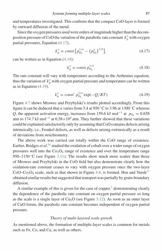
Systems forming multiple-layer scales 87
and temperatures investigated. This confirms that the compact CoO layer is formedby outward diffusion of the metal.
Since the oxygen pressures used were orders of magnitude higher than the decom-position pressure of CoO the variation of the parabolic rate constant k ′′
p with oxygenpartial pressures, Equation (4.17),
k ′′p = const.
[p1/n
O2− (
poO2
)1/n], (4.17)
can be written as in Equation (4.18):
k ′′p = const.p1/n
O2. (4.18)
The rate constant will vary with temperature according to the Arrhenius equation,thus the variation of k ′′
p with oxygen partial pressure and temperature can be writtenas in Equation (4.19).
k ′′p = const′.p1/n
O2exp(−Q/RT ) (4.19)
Figure 4.7 shows Mrowec and Przybylski’s results plotted accordingly. From thisfigure it can be deduced that n varies from 3.4 at 950 ◦C to 3.96 at 1300 ◦C whereasQ, the apparent activation energy, increases from 159.6 kJ mol−1 at pO2 = 0.658atm to 174.7 kJ mol−1 at 6.58×10⁴ atm. They further showed that these variationscould be explained satisfactorily only by assuming that CoO contains defects arisingintrinsically, i.e., Frenkel defects, as well as defects arising extrinsically as a resultof deviations from stoichiometry.
The above work was carried out totally within the CoO range of existence.Earlier, Bridges et al.36 studied the oxidation of cobalt over a wider range of oxygenpressures well into the Co3O4 range of existence and over the temperature range950–1150 ◦C (see Figure 3.11). The results show much more scatter than thoseof Mrowec and Przybylski in the CoO field but also demonstrate clearly how theoxidation-rate constant ceases to vary with oxygen pressure once the two-layerCoO–Co3O4 scale, such as that shown in Figure 4.8, is formed. Hsu and Yurek37
obtained similar results but suggested that transport was partially by grain-boundarydiffusion.
A similar example of this is given for the case of copper,5 demonstrating clearlythe dependence of the parabolic rate constant on oxygen partial pressure so longas the scale is a single layer of Cu2O (see Figure 3.12). As soon as an outer layerof CuO forms, the parabolic rate constant becomes independent of oxygen partialpressure.
Theory of multi-layered scale growth
As mentioned above, the formation of multiple-layer scales is common for metalssuch as Fe, Co, and Cu, as well as others.
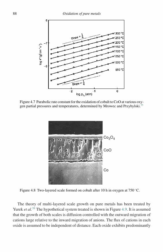
88 Oxidation of pure metals
Figure 4.7 Parabolic rate constant for the oxidation of cobalt to CoO at various oxy-gen partial pressures and temperatures, determined by Mrowec and Przybylski.35
Co3O4
CoO
Co
Figure 4.8 Two-layered scale formed on cobalt after 10 h in oxygen at 750 ◦C.
The theory of multi-layered scale growth on pure metals has been treated byYurek et al.38 The hypothetical system treated is shown in Figure 4.9. It is assumedthat the growth of both scales is diffusion controlled with the outward migration ofcations large relative to the inward migration of anions. The flux of cations in eachoxide is assumed to be independent of distance. Each oxide exhibits predominantly
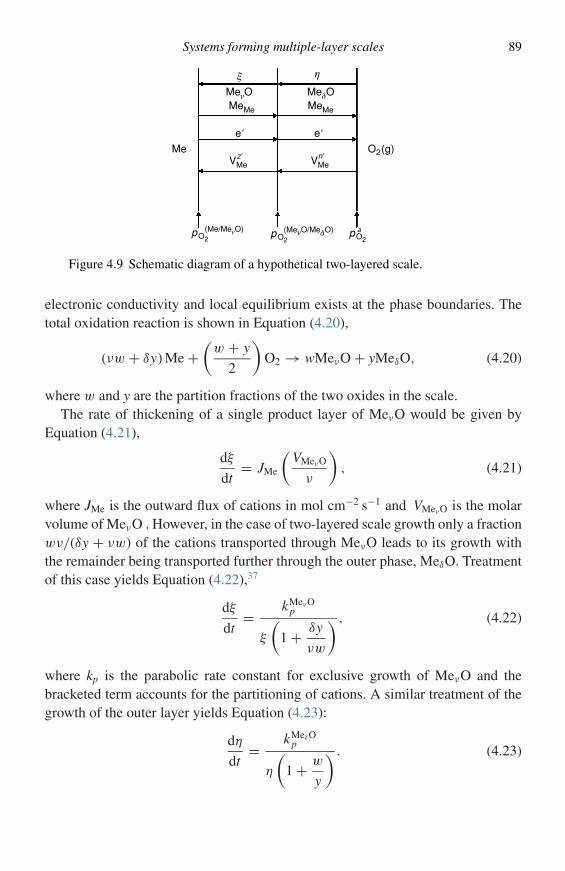
Systems forming multiple-layer scales 89
Me
pO2
O2(g)
e′e′
MeMe MeMe
MeνO
ξ η
MeδO
VMez′ VMe
n′
(Me/MeνO) pO2
(MeνO/MeδO) pO2
a
Figure 4.9 Schematic diagram of a hypothetical two-layered scale.
electronic conductivity and local equilibrium exists at the phase boundaries. Thetotal oxidation reaction is shown in Equation (4.20),
(νw + δy) Me +(
w + y
2
)O2 → wMeνO + yMeδO, (4.20)
where w and y are the partition fractions of the two oxides in the scale.The rate of thickening of a single product layer of MeνO would be given by
Equation (4.21),
dξ
dt= JMe
(VMeνO
ν
), (4.21)
where JMe is the outward flux of cations in mol cm−2 s−1 and VMeνO is the molarvolume of MeνO . However, in the case of two-layered scale growth only a fractionwν/(δy + νw) of the cations transported through MeνO leads to its growth withthe remainder being transported further through the outer phase, MeδO. Treatmentof this case yields Equation (4.22),37
dξ
dt= kMeνO
p
ξ
(1 + δy
νw
) , (4.22)
where kp is the parabolic rate constant for exclusive growth of MeνO and thebracketed term accounts for the partitioning of cations. A similar treatment of thegrowth of the outer layer yields Equation (4.23):
dη
dt= kMeδO
p
η
(1 + w
y
) . (4.23)
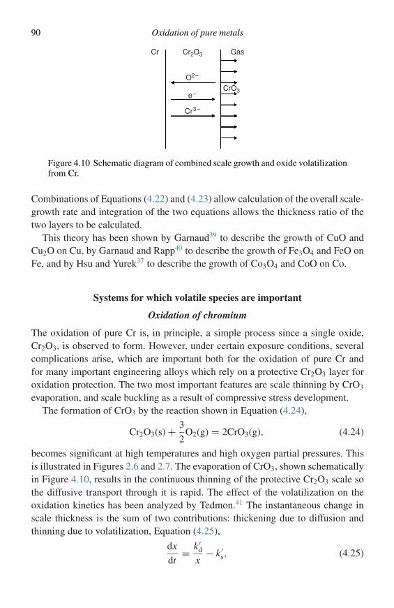
90 Oxidation of pure metals
Cr GasCr2O3
CrO3
O2−
e−
Cr3−
Figure 4.10 Schematic diagram of combined scale growth and oxide volatilizationfrom Cr.
Combinations of Equations (4.22) and (4.23) allow calculation of the overall scale-growth rate and integration of the two equations allows the thickness ratio of thetwo layers to be calculated.
This theory has been shown by Garnaud39 to describe the growth of CuO andCu2O on Cu, by Garnaud and Rapp40 to describe the growth of Fe3O4 and FeO onFe, and by Hsu and Yurek37 to describe the growth of Co3O4 and CoO on Co.
Systems for which volatile species are important
Oxidation of chromium
The oxidation of pure Cr is, in principle, a simple process since a single oxide,Cr2O3, is observed to form. However, under certain exposure conditions, severalcomplications arise, which are important both for the oxidation of pure Cr andfor many important engineering alloys which rely on a protective Cr2O3 layer foroxidation protection. The two most important features are scale thinning by CrO3
evaporation, and scale buckling as a result of compressive stress development.The formation of CrO3 by the reaction shown in Equation (4.24),
Cr2O3(s) + 3
2O2(g) = 2CrO3(g), (4.24)
becomes significant at high temperatures and high oxygen partial pressures. Thisis illustrated in Figures 2.6 and 2.7. The evaporation of CrO3, shown schematicallyin Figure 4.10, results in the continuous thinning of the protective Cr2O3 scale sothe diffusive transport through it is rapid. The effect of the volatilization on theoxidation kinetics has been analyzed by Tedmon.41 The instantaneous change inscale thickness is the sum of two contributions: thickening due to diffusion andthinning due to volatilization, Equation (4.25),
dx
dt= k ′
d
x− k ′
s, (4.25)
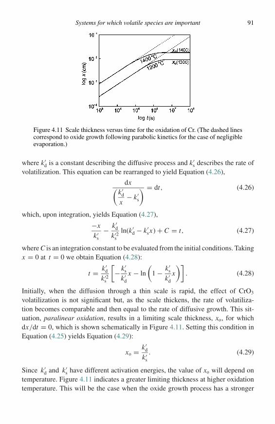
Systems for which volatile species are important 91
Figure 4.11 Scale thickness versus time for the oxidation of Cr. (The dashed linescorrespond to oxide growth following parabolic kinetics for the case of negligibleevaporation.)
where k ′d is a constant describing the diffusive process and k ′
s describes the rate ofvolatilization. This equation can be rearranged to yield Equation (4.26),
dx(k ′
d
x− k ′
s
) = dt, (4.26)
which, upon integration, yields Equation (4.27),
−x
k ′s
− k ′d
k ′2s
ln(k ′d − k ′
sx) + C = t, (4.27)
where C is an integration constant to be evaluated from the initial conditions. Takingx = 0 at t = 0 we obtain Equation (4.28):
t = k ′d
k ′2s
[− k ′
s
k ′d
x − ln
(1 − k ′
s
k ′d
x
)]. (4.28)
Initially, when the diffusion through a thin scale is rapid, the effect of CrO3
volatilization is not significant but, as the scale thickens, the rate of volatiliza-tion becomes comparable and then equal to the rate of diffusive growth. This sit-uation, paralinear oxidation, results in a limiting scale thickness, xo, for whichdx/dt = 0, which is shown schematically in Figure 4.11. Setting this condition inEquation (4.25) yields Equation (4.29):
xo = k ′d
k ′s
. (4.29)
Since k ′d and k ′
s have different activation energies, the value of xo will depend ontemperature. Figure 4.11 indicates a greater limiting thickness at higher oxidationtemperature. This will be the case when the oxide growth process has a stronger
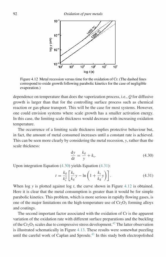
92 Oxidation of pure metals
Figure 4.12 Metal recession versus time for the oxidation of Cr. (The dashed linescorrespond to oxide growth following parabolic kinetics for the case of negligibleevaporation.)
dependence on temperature than does the vaporization process, i.e., Q for diffusivegrowth is larger than that for the controlling surface process such as chemicalreaction or gas-phase transport. This will be the case for most systems. However,one could envision systems where scale growth has a smaller activation energy.In this case, the limiting scale thickness would decrease with increasing oxidationtemperature.
The occurrence of a limiting scale thickness implies protective behaviour but,in fact, the amount of metal consumed increases until a constant rate is achieved.This can be seen more clearly by considering the metal recession, y, rather than thescale thickness:
dy
dt= kd
y+ ks. (4.30)
Upon integration Equation (4.30) yields Equation (4.31):
t = kd
k2s
[ks
kdy − ln
(1 + ks
kdy
)]. (4.31)
When log y is plotted against log t, the curve shown in Figure 4.12 is obtained.Here it is clear that the metal consumption is greater than it would be for simpleparabolic kinetics. This problem, which is more serious in rapidly flowing gases, isone of the major limitations on the high-temperature use of Cr2O3 forming alloysand coatings.
The second important factor associated with the oxidation of Cr is the apparentvariation of the oxidation rate with different surface preparations and the bucklingof the Cr2O3 scales due to compressive stress development.42 The latter observationis illustrated schematically in Figure 4.13. These results were somewhat puzzlinguntil the careful work of Caplan and Sproule.43 In this study both electropolished
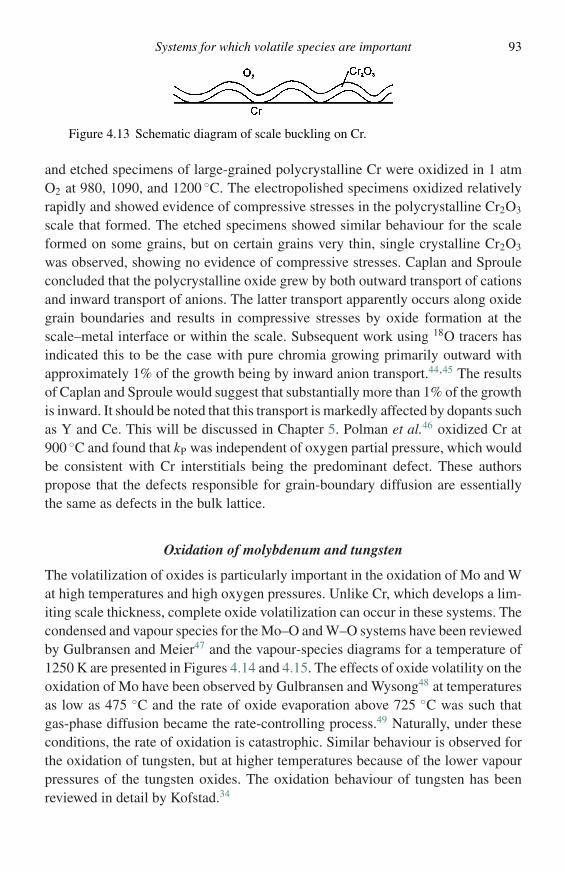
Systems for which volatile species are important 93
Figure 4.13 Schematic diagram of scale buckling on Cr.
and etched specimens of large-grained polycrystalline Cr were oxidized in 1 atmO2 at 980, 1090, and 1200 ◦C. The electropolished specimens oxidized relativelyrapidly and showed evidence of compressive stresses in the polycrystalline Cr2O3
scale that formed. The etched specimens showed similar behaviour for the scaleformed on some grains, but on certain grains very thin, single crystalline Cr2O3
was observed, showing no evidence of compressive stresses. Caplan and Sprouleconcluded that the polycrystalline oxide grew by both outward transport of cationsand inward transport of anions. The latter transport apparently occurs along oxidegrain boundaries and results in compressive stresses by oxide formation at thescale–metal interface or within the scale. Subsequent work using 18O tracers hasindicated this to be the case with pure chromia growing primarily outward withapproximately 1% of the growth being by inward anion transport.44,45 The resultsof Caplan and Sproule would suggest that substantially more than 1% of the growthis inward. It should be noted that this transport is markedly affected by dopants suchas Y and Ce. This will be discussed in Chapter 5. Polman et al.46 oxidized Cr at900 ◦C and found that kP was independent of oxygen partial pressure, which wouldbe consistent with Cr interstitials being the predominant defect. These authorspropose that the defects responsible for grain-boundary diffusion are essentiallythe same as defects in the bulk lattice.
Oxidation of molybdenum and tungsten
The volatilization of oxides is particularly important in the oxidation of Mo and Wat high temperatures and high oxygen pressures. Unlike Cr, which develops a lim-iting scale thickness, complete oxide volatilization can occur in these systems. Thecondensed and vapour species for the Mo–O and W–O systems have been reviewedby Gulbransen and Meier47 and the vapour-species diagrams for a temperature of1250 K are presented in Figures 4.14 and 4.15. The effects of oxide volatility on theoxidation of Mo have been observed by Gulbransen and Wysong48 at temperaturesas low as 475 ◦C and the rate of oxide evaporation above 725 ◦C was such thatgas-phase diffusion became the rate-controlling process.49 Naturally, under theseconditions, the rate of oxidation is catastrophic. Similar behaviour is observed forthe oxidation of tungsten, but at higher temperatures because of the lower vapourpressures of the tungsten oxides. The oxidation behaviour of tungsten has beenreviewed in detail by Kofstad.34
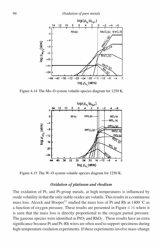
94 Oxidation of pure metals
Figure 4.14 The Mo–O system volatile-species diagram for 1250 K.
Figure 4.15 The W–O system volatile-species diagram for 1250 K.
Oxidation of platinum and rhodium
The oxidation of Pt, and Pt-group metals, at high temperatures is influenced byoxide volatility in that the only stable oxides are volatile. This results in a continuousmass loss. Alcock and Hooper50 studied the mass loss of Pt and Rh at 1400 ◦C asa function of oxygen pressure. These results are presented in Figure 4.16 where itis seen that the mass loss is directly proportional to the oxygen partial pressure.The gaseous species were identified as PtO2 and RhO2 . These results have an extrasignificance because Pt and Pt–Rh wires are often used to support specimens duringhigh-temperature oxidation experiments. If these experiments involve mass-change
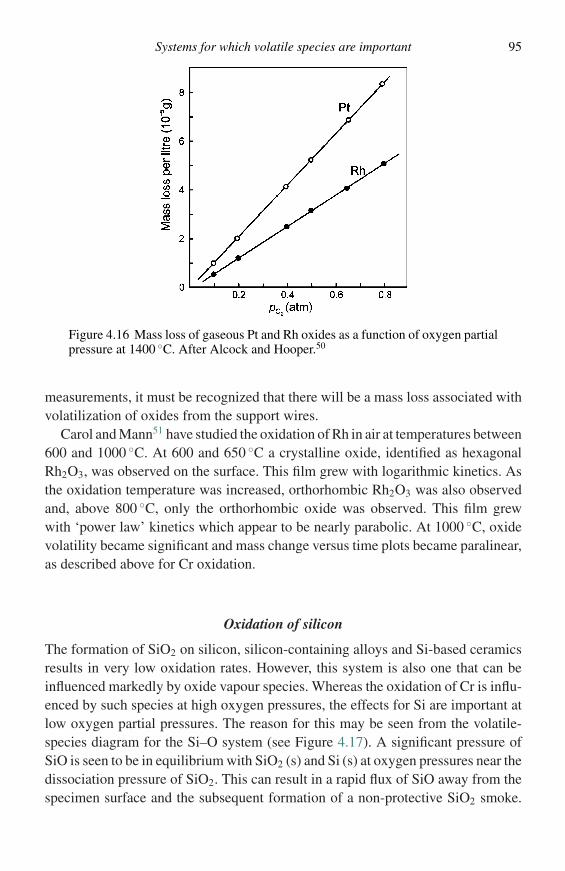
Systems for which volatile species are important 95
Figure 4.16 Mass loss of gaseous Pt and Rh oxides as a function of oxygen partialpressure at 1400 ◦C. After Alcock and Hooper.50
measurements, it must be recognized that there will be a mass loss associated withvolatilization of oxides from the support wires.
Carol and Mann51 have studied the oxidation of Rh in air at temperatures between600 and 1000 ◦C. At 600 and 650 ◦C a crystalline oxide, identified as hexagonalRh2O3, was observed on the surface. This film grew with logarithmic kinetics. Asthe oxidation temperature was increased, orthorhombic Rh2O3 was also observedand, above 800 ◦C, only the orthorhombic oxide was observed. This film grewwith ‘power law’ kinetics which appear to be nearly parabolic. At 1000 ◦C, oxidevolatility became significant and mass change versus time plots became paralinear,as described above for Cr oxidation.
Oxidation of silicon
The formation of SiO2 on silicon, silicon-containing alloys and Si-based ceramicsresults in very low oxidation rates. However, this system is also one that can beinfluenced markedly by oxide vapour species. Whereas the oxidation of Cr is influ-enced by such species at high oxygen pressures, the effects for Si are important atlow oxygen partial pressures. The reason for this may be seen from the volatile-species diagram for the Si–O system (see Figure 4.17). A significant pressure ofSiO is seen to be in equilibrium with SiO2 (s) and Si (s) at oxygen pressures near thedissociation pressure of SiO2. This can result in a rapid flux of SiO away from thespecimen surface and the subsequent formation of a non-protective SiO2 smoke.
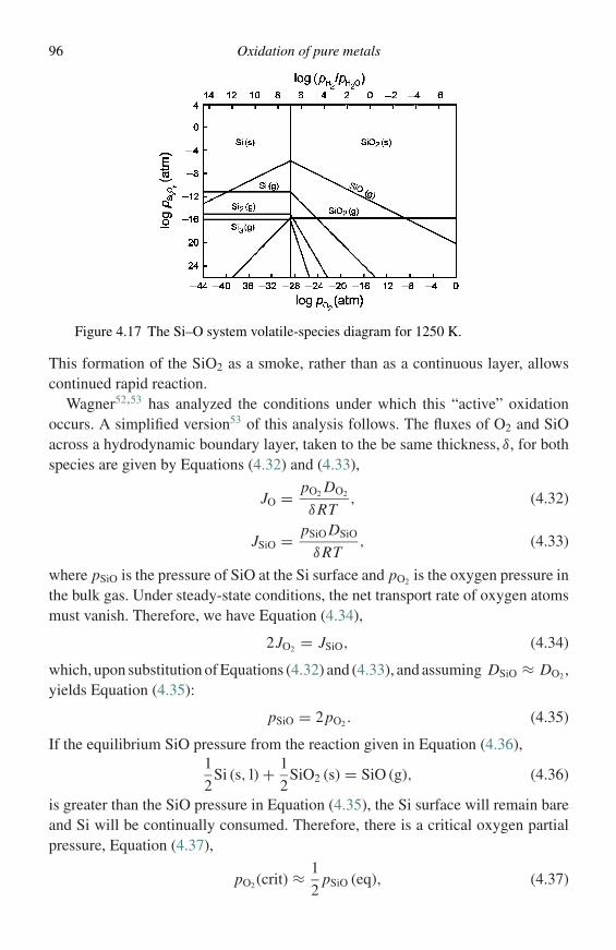
96 Oxidation of pure metals
Figure 4.17 The Si–O system volatile-species diagram for 1250 K.
This formation of the SiO2 as a smoke, rather than as a continuous layer, allowscontinued rapid reaction.
Wagner52,53 has analyzed the conditions under which this “active” oxidationoccurs. A simplified version53 of this analysis follows. The fluxes of O2 and SiOacross a hydrodynamic boundary layer, taken to the be same thickness, δ, for bothspecies are given by Equations (4.32) and (4.33),
JO = pO2 DO2
δRT, (4.32)
JSiO = pSiO DSiO
δRT, (4.33)
where pSiO is the pressure of SiO at the Si surface and pO2 is the oxygen pressure inthe bulk gas. Under steady-state conditions, the net transport rate of oxygen atomsmust vanish. Therefore, we have Equation (4.34),
2JO2 = JSiO, (4.34)
which, upon substitution of Equations (4.32) and (4.33), and assuming DSiO ≈ DO2,yields Equation (4.35):
pSiO = 2pO2 . (4.35)
If the equilibrium SiO pressure from the reaction given in Equation (4.36),1
2Si (s, l) + 1
2SiO2 (s) = SiO (g), (4.36)
is greater than the SiO pressure in Equation (4.35), the Si surface will remain bareand Si will be continually consumed. Therefore, there is a critical oxygen partialpressure, Equation (4.37),
pO2(crit) ≈ 1
2pSiO (eq), (4.37)
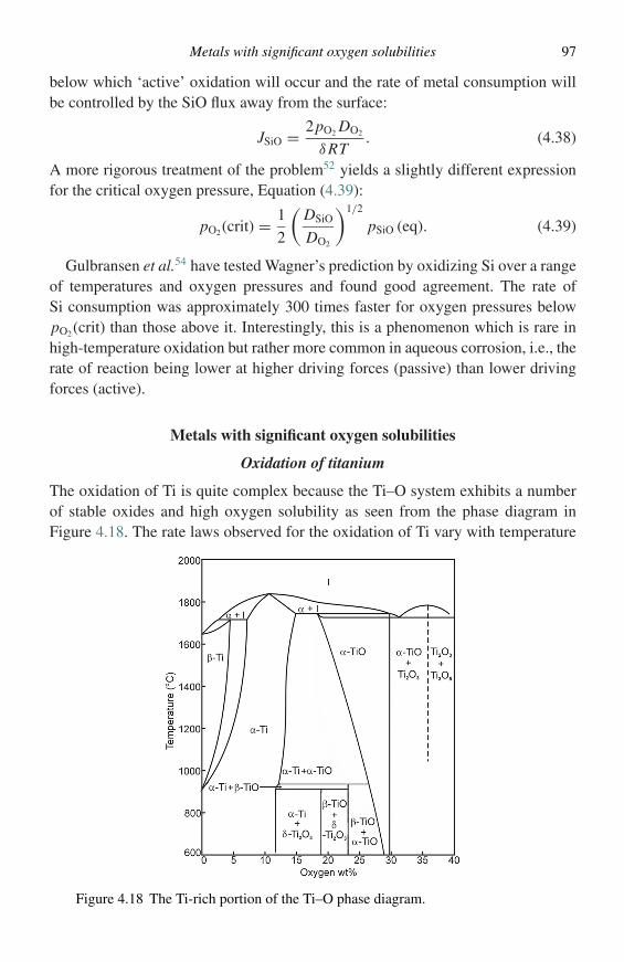
Metals with significant oxygen solubilities 97
below which ‘active’ oxidation will occur and the rate of metal consumption willbe controlled by the SiO flux away from the surface:
JSiO = 2pO2 DO2
δRT. (4.38)
A more rigorous treatment of the problem52 yields a slightly different expressionfor the critical oxygen pressure, Equation (4.39):
pO2(crit) = 1
2
(DSiO
DO2
)1/2
pSiO (eq). (4.39)
Gulbransen et al.54 have tested Wagner’s prediction by oxidizing Si over a rangeof temperatures and oxygen pressures and found good agreement. The rate ofSi consumption was approximately 300 times faster for oxygen pressures belowpO2(crit) than those above it. Interestingly, this is a phenomenon which is rare inhigh-temperature oxidation but rather more common in aqueous corrosion, i.e., therate of reaction being lower at higher driving forces (passive) than lower drivingforces (active).
Metals with significant oxygen solubilities
Oxidation of titanium
The oxidation of Ti is quite complex because the Ti–O system exhibits a numberof stable oxides and high oxygen solubility as seen from the phase diagram inFigure 4.18. The rate laws observed for the oxidation of Ti vary with temperature
Figure 4.18 The Ti-rich portion of the Ti–O phase diagram.
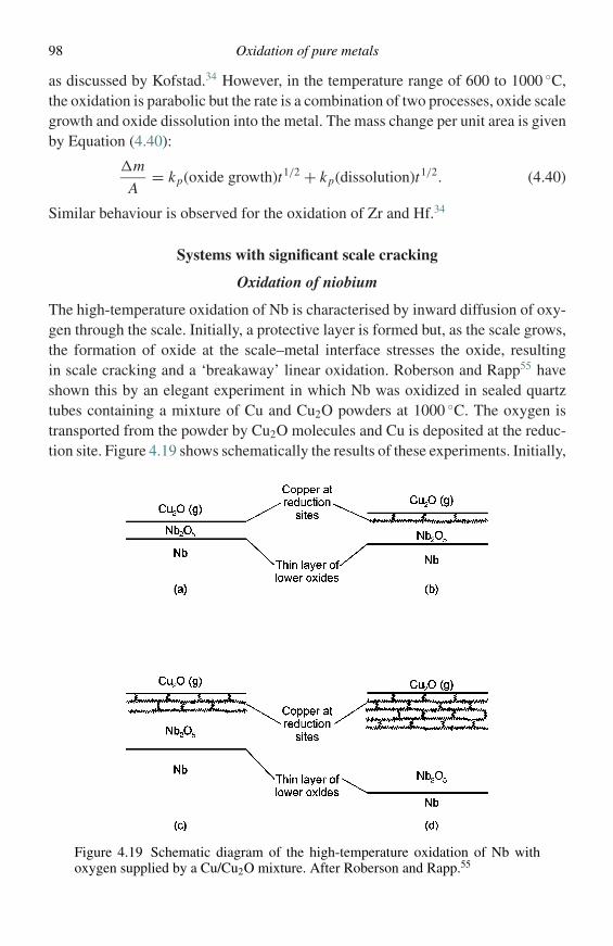
98 Oxidation of pure metals
as discussed by Kofstad.34 However, in the temperature range of 600 to 1000 ◦C,the oxidation is parabolic but the rate is a combination of two processes, oxide scalegrowth and oxide dissolution into the metal. The mass change per unit area is givenby Equation (4.40):
�m
A= kp(oxide growth)t1/2 + kp(dissolution)t1/2. (4.40)
Similar behaviour is observed for the oxidation of Zr and Hf.34
Systems with significant scale cracking
Oxidation of niobium
The high-temperature oxidation of Nb is characterised by inward diffusion of oxy-gen through the scale. Initially, a protective layer is formed but, as the scale grows,the formation of oxide at the scale–metal interface stresses the oxide, resultingin scale cracking and a ‘breakaway’ linear oxidation. Roberson and Rapp55 haveshown this by an elegant experiment in which Nb was oxidized in sealed quartztubes containing a mixture of Cu and Cu2O powders at 1000 ◦C. The oxygen istransported from the powder by Cu2O molecules and Cu is deposited at the reduc-tion site. Figure 4.19 shows schematically the results of these experiments. Initially,
Figure 4.19 Schematic diagram of the high-temperature oxidation of Nb withoxygen supplied by a Cu/Cu2O mixture. After Roberson and Rapp.55
References 99
the Cu was found at the scale–gas interface indicating the growth of a continuouslayer of Nb2O5 over lower oxides of Nb by the inward migration of oxygen. Withincreasing time, the Cu was found to occupy cracks through the outer portion ofthe scale indicating that progressive scale cracking is the cause of the accelerated,linear, oxidation. The cracking of the Nb2O5 has also been observed in situ withacoustic emission measurements.56 For example, oxidation at 600 ◦C resulted inan initial period during which the scale followed parabolic growth kinetics and nocracking was detected. After an incubation period of 15 min, significant crackingwas detected by acoustic emission and the oxidation kinetics rapidly became linear.Similar oxidation behaviour is also observed for Ta. As a result, neither Nb nor Tacan be used for any extended period at elevated temperature without a protectivecoating.
References
1. F. S. Pettit, R. Yinger, and J. B. Wagner, Acta Met., 8 (1960), 617.2. J. C. Yang, M. Yeadon, B. Kolasa, and J. M. Gibson, Scripta Mater., 38 (1998), 1237.3. J. Romanski, Corros. Sci., 8 (1968), 67; 89.4. A. Bruckmann, in Reaction Kinetics in Heterogeneous Chemical Systems, ed. P.
Barret, Amsterdam Elsevier, 1975, p. 409.5. S. Mrowec and A. Stoklosa, Oxid. Metals, 3 (1971), 291.6. O. Kubaschewski and O. van Goldbeck, Z. Metallkunde, 39 (1948), 158.7. Y. Matsunaga, Japan Nickel Rev., 1 (1933), 347.8. W. J. Moore, J. Chem. Phys., 19 (1951), 255.9. E. A. Gulbransen and K. F. Andrew, J. Electrochem. Soc., 101 (1954), 128.
10. W. Philips, J. Electrochem. Soc., 110 (1963), 1014.11. G. C. Wood and I. G. Wright, Corr. Sci., 5 (1965), 841.12. N. Birks and H. Rickert, J. Inst. Metals, 91 (1962), 308.13. B. Ilschner and H. Pfeiffer, Naturwissenschaft, 40 (1953), 603.14. L. Czerski and F. Franik, Arch. Gorn. Hutn., 3 (1955), 43.15. D. Caplan, M. J. Graham, and M. Cohen, J. Electrochem. Soc., 119 (1978), 1205.16. M. J. Graham, D. Caplan, and R. J. Hussey, Can. Met. Quart., 18 (1979), 283.17. S. Mrowec and T. Werber, Gas Corrosion of Metals, Springfield, VA, US Department
of Commerce, National Technical Information Service, 1978, p. 383.18. A. Atkinson and D. W. Smart, J. Electrochem. Soc., 135 (1988), 2886.19. K. Fueki and J. B. Wagner, J. Electrochem. Soc., 112 (1965), 384.20. C. Wagner and K. Grunewald, Z. Phys. Chem., 40B (1938), 455.21. K. Wefers and C. Misra, AlCOA Technical Paper 19, Pittsburgh, PA, Aluminium
Company of America, 1987.22. P. Liu and J. Skogsmo, Acta Crystallogr., B47 (1991), 425.23. K. Shimizu, K. Kobayashi, G. E. Thompson, and G. C. Wood, Oxid. Met., 36 (1991),
1.24. K. Shimizu, R. C. Furneaux, G. E. Thompson, et al., Oxid. Met, 35 (1991), 427.25. J. I. Eldridge, R. J. Hussey, D. F. Mitchell, and M. J. Graham, Oxid. Met., 30 (1988),
301.26. H. J. Engell, Archiv. Eisenhuttenwesen, 28 (1957), 109.
100 Oxidation of pure metals
27. H. J. Engell, Acta met., 6 (1958), 439.28. M. H. Davies, M. T. Simnad, and C. E. Birchenall, J. Met., 3 (1951), 889.29. D. J. M. Deven, J. P. Shelton, and J. S. Anderson, J. Chem. Soc., 2 (1948), 1729.30. A. Bruckmann and G. Simkovich, Corr. Sci., 12 (1972), 595.31. W. Schwenk and A. Rahmel, Oxid. Met., 25 (1986), 293.32. R. H. Jutte, B. J. Kooi, M. A. J. Somers, and E. J. Mittemeijer, Oxid. Met., 48 (1997),
87.33. S. Mrowec and K. Przybylski, Oxid. Met., 11 (1977), 383.34. P. Kofstad, High Temperature Oxidation of Metals, New York, Wiley, 1966.35. S. Mrowec and K. Przybylski, Oxid. Met., 11 (1977), 365.36. D. W. Bridges, J. P. Baur, and W. M. Fassel, J. Electrochem. Soc., 103 (1956), 619.37. H. S. Hsu and G. J. Yurek, Oxid. Met., 17 (1982), 55.38. G. J. Yurek, J. P. Hirth, and R. A. Rapp, Oxid. Met., 8 (1974), 265.39. G. Garnaud, Oxid. Met., 11 (1977), 127.40. G. Garnaud and R. A. Rapp, Oxid. Met., 11 (1977), 193.41. C. S. Tedmon, J. Electrochem. Soc., 113 (1966), 766.42. D. Caplan, A. Harvey, and M. Cohen, Corr. Sci., 3 (1963), 161.43. D. Caplan and G. I. Sproule, Oxid. Met., 9 (1975), 459.44. R. J. Hussey and M. J. Graham, Oxid. Met., 45 (1996), 349.45. C. M. Cotell, G. J. Yurek, R. J. Hussey, D. J. Mitchell, and M. J. Graham, Oxid. Met.,
34 (1990), 173.46. E. A. Polman, T. Fransen, and P. J. Gellings, Oxid. Met., 32 (1989), 433.47. E. A. Gulbransen and G. H. Meier, Mechanisms of oxidation and hot corrosion of
metals and alloys at temperatures of 1150 to 1450 K under flow. In Proceedings of10th Materials Research Symposium, National Bureau of Standards SpecialPublications 561, 1979, p. 1639.
48. E. A. Gulbransen and W. S. Wysong, TAIME, 175 (1948), 628.49. E. A. Gulbransen, K. F. Andrew, and F. A. Brassart, J. Electrochem. Soc., 110
(1963), 952.50. C. B. Alcock and G. W. Hooper, Proc. Roy. Soc., 254A (1960), 551.51. L. A. Carol and G. S. Mann, Oxid. Met., 34 (1990), 1.52. C. Wagner, J. Appl. Phys., 29 (1958), 1295.53. C. Wagner, Corr. Sci., 5 (1965), 751.54. E. A. Gulbransen, K. F. Andrew, and F. A. Brassart, J. Electrochem. Soc., 113
(1966), 834.55. J. A. Roberson and R. A. Rapp, TAIME, 239 (1967), 1327.56. R. A. Perkins and G. H. Meier, Acoustic emission studies of high temperature
oxidation. In High Temperature Materials Chemistry, eds. Z. A. Munir and D.Cubicciotti, New York, NY, Electrochemical Society, 1983, p. 176.
5
Oxidation of alloys
Introduction
Many of the factors described for the oxidation of pure metals also apply to theoxidation of alloys. However, alloy oxidation is generally much more complex asa result of some, or all, of the following.� The metals in the alloy will have different affinities for oxygen reflected by the different
free energies of formation of the oxides.� Ternary and higher oxides may be formed.� A degree of solid solubility may exist between the oxides.� The various metal ions will have different mobilities in the oxide phases.� The various metals will have different diffusivities in the alloy.� Dissolution of oxygen into the alloy may result in sub-surface precipitation of oxides of
one or more alloying elements (internal oxidation).
This chapter describes the major effects occurring in alloy oxidation and theirrelation to the above factors. No attempt has been made to provide a completesurvey of the extensive literature on this subject, rather, examples which illus-trate the important fundamentals are presented. This is done by first classifyingthe types of reactions which occur, and then describing additional factors which havesignificant influences on the oxidation process. Subsequent chapters will describethe oxidation of alloys in complex environments, such as those involving mixedgases, liquid deposits, and erosive conditions and the use of coatings for oxidationprotection. Previous reviews of alloy oxidation include those by Kubaschewskiand Hopkins,1 Hauffe,2 Benard,3 Pfeiffer and Thomas,4 Birchenall,5 Mrowec andWerber,6 Kofstad,7 and Beranger, Colson and Dabosi.8
Classification of reaction types
Wagner9 has presented a lucid categorization of simple types of alloy oxidationaccording to the reaction morphologies. The classification presented here is a
101
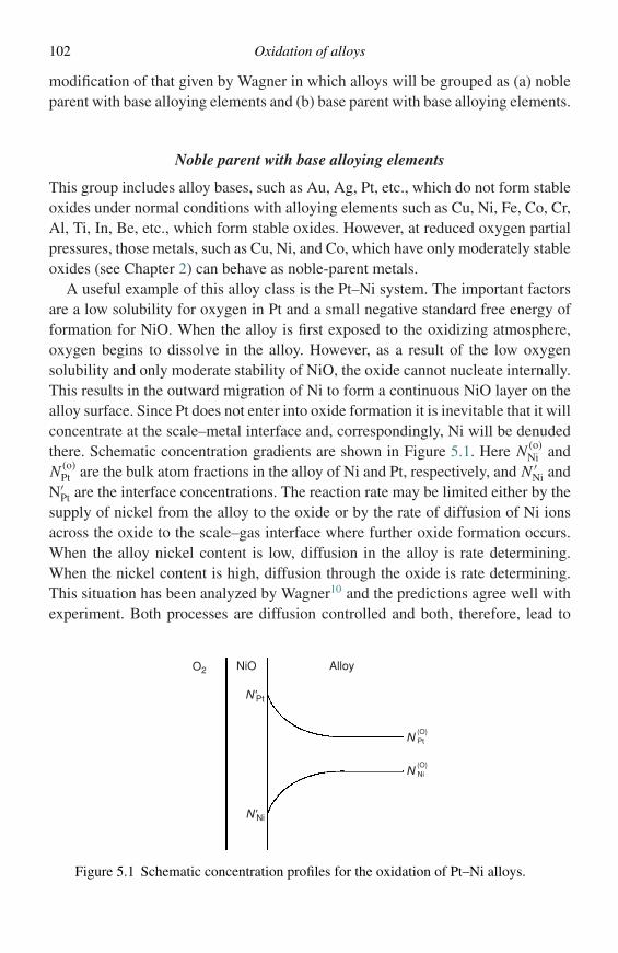
102 Oxidation of alloys
modification of that given by Wagner in which alloys will be grouped as (a) nobleparent with base alloying elements and (b) base parent with base alloying elements.
Noble parent with base alloying elements
This group includes alloy bases, such as Au, Ag, Pt, etc., which do not form stableoxides under normal conditions with alloying elements such as Cu, Ni, Fe, Co, Cr,Al, Ti, In, Be, etc., which form stable oxides. However, at reduced oxygen partialpressures, those metals, such as Cu, Ni, and Co, which have only moderately stableoxides (see Chapter 2) can behave as noble-parent metals.
A useful example of this alloy class is the Pt–Ni system. The important factorsare a low solubility for oxygen in Pt and a small negative standard free energy offormation for NiO. When the alloy is first exposed to the oxidizing atmosphere,oxygen begins to dissolve in the alloy. However, as a result of the low oxygensolubility and only moderate stability of NiO, the oxide cannot nucleate internally.This results in the outward migration of Ni to form a continuous NiO layer on thealloy surface. Since Pt does not enter into oxide formation it is inevitable that it willconcentrate at the scale–metal interface and, correspondingly, Ni will be denudedthere. Schematic concentration gradients are shown in Figure 5.1. Here N (o)
Ni andN (o)
Pt are the bulk atom fractions in the alloy of Ni and Pt, respectively, and N ′Ni and
N′Pt are the interface concentrations. The reaction rate may be limited either by the
supply of nickel from the alloy to the oxide or by the rate of diffusion of Ni ionsacross the oxide to the scale–gas interface where further oxide formation occurs.When the alloy nickel content is low, diffusion in the alloy is rate determining.When the nickel content is high, diffusion through the oxide is rate determining.This situation has been analyzed by Wagner10 and the predictions agree well withexperiment. Both processes are diffusion controlled and both, therefore, lead to
O2 NiO
N'Pt
N'Ni
Alloy
N(O)Pt
N(O)Ni
Figure 5.1 Schematic concentration profiles for the oxidation of Pt–Ni alloys.
Classification of reaction types 103
(kp)Ni
kp
NNi
Figure 5.2 Effect of nickel on the parabolic rate constant for the oxidation of Pt–Nialloys.
parabolic kinetics. As the nickel content is increased, the parabolic rate constantapproaches values typical of pure nickel as shown schematically in Figure 5.2. Thebulk nickel content below which diffusion in the alloy controls may be calculated byequating the fluxes arriving at the alloy–oxide interface to that required to maintainthe growth of the oxide. Here we consider the general case of a system A–B whereA represents the noble component and BOν is the oxide being formed:
JB = DB
Vm
(∂ NB
∂x
)x=0
= 1
ν· 1
2· k1/2
p
MOt−1/2. (5.1)
The concentration gradient in Equation (5.1) may be evaluated by differentiatingEquation (A19) from Appendix A, with N (S)
B being taken as zero, leading to theresult shown in Equation (5.2):
N (o)B = Vm
32ν
(πkp
DB
)1/2
. (5.2)
When the scale growth is controlled by diffusion in the alloy, the scale–alloyinterface can become unstable as illustrated in Figure 5.3. Since any inward protu-berance of the scale–alloy interface will shorten the diffusion distance across thezone depleted in B, such a protuberance will grow and result in a wavy scale–alloyinterface. This problem has been described by Wagner.11 Similar considerationsapply to the scale–gas interface, which can develop oxide whiskers if gas-phasediffusion of oxidant to the surface controls the rate. Rickert12 has shown this to bethe case for the reaction of silver and sulphur using the experiment shown schemat-ically in Figure 5.4. A silver specimen was placed in one end of a sealed, evacuatedtube and a quantity of sulphur was placed in the other. The tube was heated to 400 ◦Cin an inclined furnace. Sulphur transport through the vapour caused an Ag2S layerto grow on the portion of silver nearest the sulphur. However, as the S was depleted
104 Oxidation of alloys
O2
BO
B
A–BConstant aB
Figure 5.3 Schematic representation of a non-planar scale–alloy interface resultingfrom rate control by alloy interdiffusion.
Figure 5.4 Whisker growth in the reaction between Ag and S resulting from gas-phase diffusion control.
from the vapour by this reaction, the rate of transport to the far end of the specimenbecame rate controlling so that Ag2S whiskers grew on this end as indicated inFigure 5.4.
Silver-base alloys containing less noble solutes, such as In or Al, representanother useful case in this classification. In this case the solubility of oxygen in Agis significant so that, for dilute alloys, internal oxidation can occur.
Internal oxidation
Internal oxidation is the process in which oxygen diffuses into an alloy and causessub-surface precipitation of the oxides of one or more alloying elements. It hasbeen the subject of reviews by Rapp,13 Swisher,14 Meijering,15 and Douglass.16
The necessary conditions for the occurrence of the phenomenon are thefollowing.

Classification of reaction types 105
(1) The value of �Go of formation (per mole O2) for the solute metal oxide, BOν , must bemore negative than �Go of formation (per mole O2) for the base metal oxide.
(2) The value of �G for the reaction B + νO = BOν must be negative. Therefore, the basemetal must have a solubility and diffusivity for oxygen which is sufficient to establishthe required activity of dissolved oxygen O at the reaction front.
(3) The solute concentration of the alloy must be lower than that required for the transitionfrom internal to external oxidation.
(4) No surface layer must prevent the dissolution of oxygen into the alloy at the start ofoxidation.
The process of internal oxidation occurs in the following manner. Oxygen dis-solves in the base metal (either at the external surface of the specimen or at thealloy–scale interface if an external scale is present) and diffuses inward throughthe metal matrix containing previously precipitated oxide particles. The criticalactivity product, aBaν
O, for the nucleation of precipitates is established at a reactionfront (parallel to the specimen surface) by the inward-diffusing oxygen and theoutward diffusion of solute. Nucleation of the oxide precipitate occurs and a givenprecipitate grows until the reaction front moves forward and depletes the supply ofsolute B arriving at the precipitate. Subsequent precipitate growth occurs only bycapillarity-driven coarsening (Ostwald ripening).
Kinetics
The rate of internal oxidation will be derived here for a planar specimen geometryusing the quasi-steady-state approximation. The results of similar derivations forcylindrical and spherical specimens will be presented. A more rigorous derivationof the kinetics of internal oxidation is presented in Appendix B.
Consider a planar specimen of a binary alloy A–B in which B is a dilute solute,which forms a very stable oxide. Assume the ambient oxygen pressure is too lowto oxidize A but high enough to oxidize B (see Figure 5.5).
The quasi-steady approximation requires the assumption that the dissolved oxy-gen concentration varies linearly across the zone of internal oxidation. Therefore,the oxygen flux through the internal oxidation zone (IOZ) is given by Fick’s firstlaw as Equation (5.3),
J = dm
dt= DO
N (S)O
X Vm(mol cm−2s−1), (5.3)
where N (S)O is the oxygen solubility in A (atom fraction), Vm is the molar volume
of the solvent metal or alloy (cm3 mol−1), and DO is the diffusivity of oxygenin A (cm2 s−1). If counter-diffusion of solute B is assumed to be negligible, theamount of oxygen accumulated in the IOZ per unit area of reaction front is given by
106 Oxidation of alloys
Figure 5.5 Simplified concentration profiles for the internal oxidation of A–B.
Equation (5.4),
m = N (o)B νX
Vm(mol cm−2) (5.4)
where N (o)B is the initial solute concentration. Differentiation of Equation (5.4) with
respect to time gives an alternate expression for the flux:
dm
dt= N (o)
B ν
Vm
dX
dt. (5.5)
Equating Equations (5.3) and (5.5),
DON (S)
O
X Vm= N (o)
B ν
Vm
dX
dt, (5.6)
and rearranging Equation (5.6) gives Equation (5.7):
XdX = N (S)O DO
νN (o)B
dt. (5.7)
Integration of Equation (5.7), assuming X = 0 at t = 0, yields Equation (5.8),
1
2X2 = N (S)
O DO
νN (o)B
t, (5.8)
or Equation (5.9):
X =[
2N (S)O DO
νN (o)B
t
]1/2
. (5.9)
Classification of reaction types 107
Figure 5.6 Optical micrograph showing the microstructure of a Cu–0.47 wt% Tialloy internally oxidized at 800 ◦C for 97 h.
The latter gives the penetration depth of the internal oxidation zone as a functionof oxidation time. The following points concerning Equation (5.9) are of interest.
(1) The penetration depth has a parabolic time dependence, X ∝ t1/2.(2) The penetration depth for a fixed time is inversely proportional to the square root of the
atom fraction of solute in the bulk alloy.(3) Careful measurements of the front penetration as a function of time for an alloy of
known solute concentration can yield a value for the solubility–diffusivity product,N (S)
O DO (permeability) for oxygen in the matrix metal.
The results of a similar derivation for a cylindrical specimen14 yield Equation(5.10),
(r1)2
2− (r2)2 ln
(r1
r2
)+ 1
2= 2N (S)
O DO
νN (o)B
t, (5.10)
and for a spherical specimen,14 Equation (5.11),
(r1)2
3− (r2)2 + 2
3
(r2)3
(r1)= 2N (S)
O DO
νN (o)B
t, (5.11)
where r1 is the specimen radius and r2 is the radius of the unoxidized alloy core.Figure 5.6 shows a polished and etched cross-section of an internally oxidized
Cu–Ti cylinder showing the penetration of the internal oxidation zone.17 The TiO2
particles are too small to resolve in the optical microscope. Measurements of r2
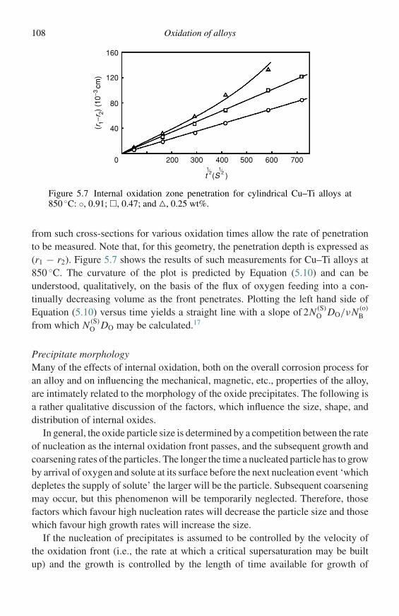
108 Oxidation of alloys
160
120
80
40(r1−r
2) (
10−3
cm)
0 200 300 400 500 600 700
t (S )1
21
2
Figure 5.7 Internal oxidation zone penetration for cylindrical Cu–Ti alloys at850 ◦C: ◦, 0.91; �, 0.47; and �, 0.25 wt%.
from such cross-sections for various oxidation times allow the rate of penetrationto be measured. Note that, for this geometry, the penetration depth is expressed as(r1 − r2). Figure 5.7 shows the results of such measurements for Cu–Ti alloys at850 ◦C. The curvature of the plot is predicted by Equation (5.10) and can beunderstood, qualitatively, on the basis of the flux of oxygen feeding into a con-tinually decreasing volume as the front penetrates. Plotting the left hand side ofEquation (5.10) versus time yields a straight line with a slope of 2N (S)
O DO/νN (o)B
from which N (S)O DO may be calculated.17
Precipitate morphologyMany of the effects of internal oxidation, both on the overall corrosion process foran alloy and on influencing the mechanical, magnetic, etc., properties of the alloy,are intimately related to the morphology of the oxide precipitates. The following isa rather qualitative discussion of the factors, which influence the size, shape, anddistribution of internal oxides.
In general, the oxide particle size is determined by a competition between the rateof nucleation as the internal oxidation front passes, and the subsequent growth andcoarsening rates of the particles. The longer the time a nucleated particle has to growby arrival of oxygen and solute at its surface before the next nucleation event ‘whichdepletes the supply of solute’ the larger will be the particle. Subsequent coarseningmay occur, but this phenomenon will be temporarily neglected. Therefore, thosefactors which favour high nucleation rates will decrease the particle size and thosewhich favour high growth rates will increase the size.
If the nucleation of precipitates is assumed to be controlled by the velocity ofthe oxidation front (i.e., the rate at which a critical supersaturation may be builtup) and the growth is controlled by the length of time available for growth of
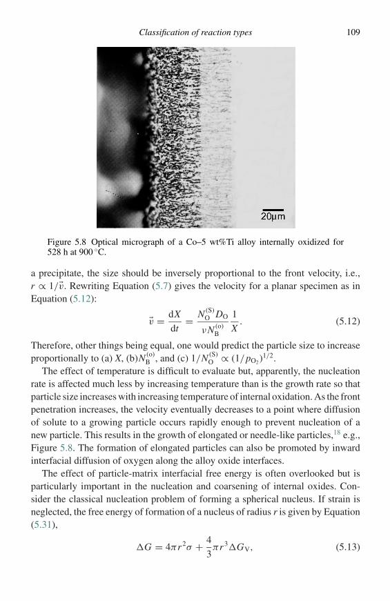
Classification of reaction types 109
Figure 5.8 Optical micrograph of a Co–5 wt%Ti alloy internally oxidized for528 h at 900 ◦C.
a precipitate, the size should be inversely proportional to the front velocity, i.e.,r ∝ 1/v. Rewriting Equation (5.7) gives the velocity for a planar specimen as inEquation (5.12):
v = dX
dt= N (S)
O DO
νN (o)B
1
X. (5.12)
Therefore, other things being equal, one would predict the particle size to increaseproportionally to (a) X, (b)N (o)
B , and (c) 1/N (S)O ∝ (1/pO2)
1/2.The effect of temperature is difficult to evaluate but, apparently, the nucleation
rate is affected much less by increasing temperature than is the growth rate so thatparticle size increases with increasing temperature of internal oxidation. As the frontpenetration increases, the velocity eventually decreases to a point where diffusionof solute to a growing particle occurs rapidly enough to prevent nucleation of anew particle. This results in the growth of elongated or needle-like particles,18 e.g.,Figure 5.8. The formation of elongated particles can also be promoted by inwardinterfacial diffusion of oxygen along the alloy oxide interfaces.
The effect of particle-matrix interfacial free energy is often overlooked but isparticularly important in the nucleation and coarsening of internal oxides. Con-sider the classical nucleation problem of forming a spherical nucleus. If strain isneglected, the free energy of formation of a nucleus of radius r is given by Equation(5.31),
�G = 4πr2σ + 4
3πr3�GV, (5.13)

110 Oxidation of alloys
4πr2σ
∆G∗
r ∗ r
∆G
G
πr 3∆Gv43
−
+
Figure 5.9 Schematic plot of free energy versus radius of a nucleating particle.
where σ is the specific interfacial free energy and �GV is the free-energy changeper unit volume of precipitate formed during the reaction. The surface and volumeterms, along with �G, are plotted as a function of r in Figure 5.9. Nuclei with radiigreater than r
∗will tend to grow spontaneously. At r∗ we have Equation (5.14),
d�G
dr= 8πr∗σ + 4πr∗2�GV = 0, (5.14)
which may be solved for r∗ as in Equation (5.15):
r∗ = −2σ
�GV. (5.15)
Substitution into Equation (5.13) yields �G∗, the height of the activation barrier tonucleation:
�G∗ = 4π4σ 3
�G2V
− 4
3π
8σ 3
�G3V
�GV
=(
16 − 32
3
)π
σ 3
�G2V
= 16
3π
σ 3
�G2V
. (5.16)
It is this value (�G∗) which enters into the nucleation rate as calculated fromabsolute reaction-rate theory, Equation (5.17),
J = ωC∗ = ωCo exp(−�G∗/RT ), (5.17)
where Co is the concentration of reactant molecules, C∗ is the concentration ofcritical nuclei, and ω is the frequency with which atoms are added to the criticalnucleus. Clearly, since the nucleation rate is proportional to the exponential of aquantity, which in turn depends on the cube of the surface free energy, this parameterwill have a drastic effect on the nucleation, and particle size will increase with
Classification of reaction types 111
increasing σ . This influence will be felt further in the coarsening of the particlessince the interfacial free energy is the driving force for this process.
In a similar manner the relative stability of the internal oxide, �G◦, will influence�GV with more stable oxides resulting in higher nucleation rates and smallerparticles.
In summary, the size of internal oxides will be determined by a number of factorswith larger particles forming for:
(1) deeper front penetrations, X(2) higher solute concentrations, N (o)
B
(3) lower oxygen solubilities, i.e., lower pO2
(4) higher temperature(5) higher particle-matrix interfacial free energies(6) less stable oxides.
These predictions have been born out in a number of studies of particle morphologyavailable in the literature.17–20 However, the internal oxidation process is quitecomplex and many systems show deviations from the simple analysis providedabove. Douglass16 has described these phenomena which include the following.
(1) Accelerated transport along the interfaces between internal oxides and the alloy matrixproducing oxide needles and deeper penetrations than those predicted from Equation(5.9).
(2) Preferential formation of internal oxides on alloy grain boundaries often with zonesadjacent to the boundary which are denuded of precipitates.
(3) Alternating bands of internal oxide particles running parallel to the specimen surface.(4) Extrusion of parent metal from the internal oxidation zone to form pure metal nodules
on the surface.(5) Formation of solute-oxygen clusters containing more than the stoichiometric oxygen
concentration.
Transition from internal to external oxidationConsideration of Equation (5.12) shows that the penetration velocity of the internaloxidation zone decreases with increasing N (o)
B and decreasing N (S)O . Thus there will
be a limiting concentration of solute in the alloy above which the outward diffusionof B will be rapid enough to form a continuous blocking layer of BOν and stopinternal oxidation (shown schematically in Figure 5.10). This transition to externaloxidation is the basis for the design of Fe-, Ni-, and Co-base engineering alloys.These contain a sufficiently high concentration of a solute (e.g., Cr, Al, or Si) toproduce an external layer of a stable, slowly growing oxide (e.g., Cr2O3, Al2O3,or SiO2), which prevents oxidation of the parent metal. This process, known asselective oxidation, will be discussed further but at this point the fundamentals ofthe transition from internal to external oxidation must be considered. The analysis of
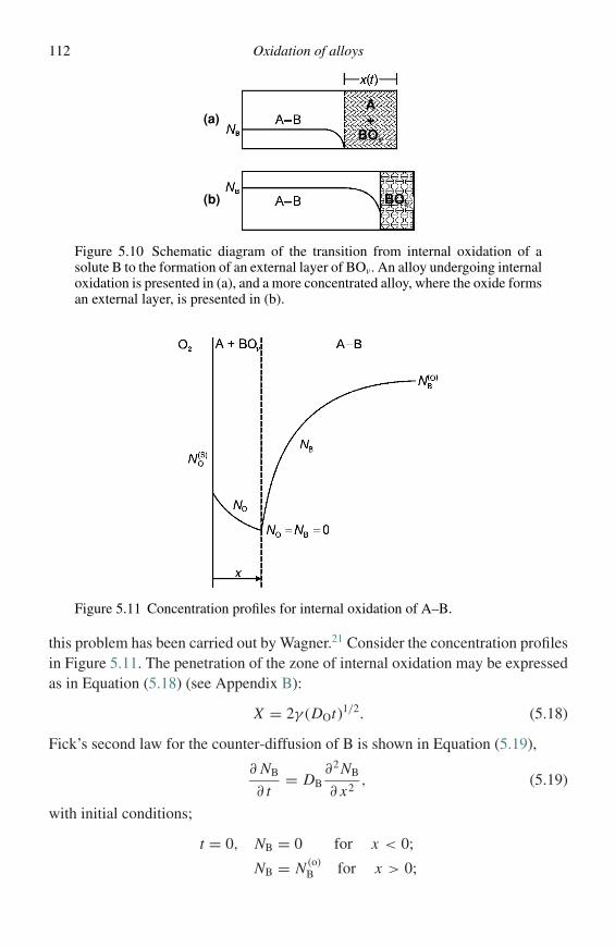
112 Oxidation of alloys
A+
BOν
BOν
(a)
(b)
Figure 5.10 Schematic diagram of the transition from internal oxidation of asolute B to the formation of an external layer of BOv. An alloy undergoing internaloxidation is presented in (a), and a more concentrated alloy, where the oxide formsan external layer, is presented in (b).
Figure 5.11 Concentration profiles for internal oxidation of A–B.
this problem has been carried out by Wagner.21 Consider the concentration profilesin Figure 5.11. The penetration of the zone of internal oxidation may be expressedas in Equation (5.18) (see Appendix B):
X = 2γ (DOt)1/2. (5.18)
Fick’s second law for the counter-diffusion of B is shown in Equation (5.19),
∂ NB
∂ t= DB
∂2 NB
∂ x2, (5.19)
with initial conditions;
t = 0, NB = 0 for x < 0;
NB = N (o)B for x > 0;
Classification of reaction types 113
and boundary conditions:
t = t, NB = 0 for x = X ;
NB = N (o)B for x = ∞.
The solution to Equation (5.19), therefore, becomes that given in Equation (5.20),
NB(x, t) = N (o)B
1 −
erfc
(x
2(DBt)1/2
)erfc(θ1/2γ )
, (5.20)
where θ = DO/DB.If f represents the mole fraction of BOν in the internal oxidation zone and Vm the
molar volume of the alloy, then f/Vm will be the concentration in moles per volumeand the number of moles in a volume element, AdX, will be (f/Vm)AdX, where Ais the cross-sectional area for diffusion. This quantity must be equal to the numberof moles of B arriving at x = X in the time dt by diffusion from within the sample,i.e., from x > X . Therefore, we obtain Equation (5.21):
f AdX
Vm=
[ADB
Vm
∂ NB
∂ x
]dt, (5.21)
Substitution of Equations (5.18) and (5.20) into Equation (5.21) yields an enrich-ment factor of α, Equation (5.22):
α = f
N (o)B
= 1
γπ1/2
(DB
DO
)1/2 exp(−γ 2θ )
erfc(γ θ1/2). (5.22)
For the case of interest here, N (S)O DO << N (o)
B DB, i.e., the oxygen permeability issignificantly less than the corresponding product for B, the product γ θ1/2<< 1 andγ is given by Equation (B20) from Appendix B. Therefore, α may be written as inEquation (5.23):
α ≈ 2ν
π
[N (o)
B DB
N (S)O DO
]. (5.23)
When α is large, we expect the accumulation and lateral growth of the internaloxides to form a continuous layer, i.e., the transition to external oxidation. Figure5.12 shows this occurring in a Co–7.5 wt% Ti alloy.18 Wagner states that, when thevolume fraction of oxide, g = f (Vox/Vm), reaches a critical value, g∗, the transitionfrom internal to external scale formation should occur. Insertion of f , in terms ofg∗, in α in Equation (5.23) then gives the criterion for external oxidation as shown
114 Oxidation of alloys
Figure 5.12 Optical micrograph showing transition from internal to external oxi-dation in a Co–7.5 wt% Ti alloy oxidized for 528 h at 900 ◦C.
in Equation (5.24):
N (o)B >
[π g∗
2νN (S)
O
DOVm
DBVox
]1/2
. (5.24)
The latter enables prediction of how changing exposure conditions will affect theconcentration of solute required to produce an external scale. Those conditionsthat decrease the inward flux of oxygen, e.g., lower N (S)
O (i.e. lowerpO2) and thosethat increase the outward flux of B, e.g., cold working the alloy (increasing DB
by increasing the contribution of short-circuit diffusion) will allow the transitionto external oxidation to occur at lower solute concentrations. Rapp22 has tested theWagner theory for Ag–In alloys. It was found that at pO2 = 1 atm and T = 550 ◦C thetransition occurred for g∗ = 0.3 (NIn = 0.16). Rapp then used this value to predictthe effect of reduced pO2 (reduced N (S)
O ) on the In concentration required for thetransition. The agreement between experiment and Equation (5.24) was excellent.Rapp’s experiments also gave an indirect verification of the effect of increased DB,caused by cold work, on the transition. Specimens containing only 6.8 at% In wereobserved to undergo the transition to external In2O3 formation around scribe marksunder exposure conditions that required 15 at% In to produce the transition onundeformed surfaces.
An additional factor which can have a pronounced influence on the transition isthe presence of a second solute whose oxide has a stability intermediate betweenthat of A and B. If the pO2 is great enough to form the oxide of the second solute thiswill, in effect, decrease the inward flux of oxygen and allow external formation of
Base parent with base-alloying elements 115
BOν at lower concentrations of B.23 This concept is often referred to as secondarygettering. Wagner observed the effect for Cu–Zn–Al alloys23 and Pickering obtainedsimilar results for Ag–Zn–Al alloys.24 In the latter experiments Ag–3 at% Al alloyswere found to oxidize internally while, under the same conditions, a Ag–21 at% Zn–3 at% Al alloy produced an external Al2O3 scale. The secondary getter concept isbased essentially on the second solute decreasing N (S)
O . However, explanation of theeffect should actually consider the effect on all of the terms in Equation (5.24).25,26
Nevertheless, the concept has proved useful in the design of high-temperature alloyssince the element which provides protection by selective oxidation (e.g., Al) oftenhas detrimental effects on other alloy properties, particularly mechanical properties,and should, in these cases, be held at as low a concentration as is feasible. Thisconcept has led to the development of the M–Cr–Al (M = Fe, Ni, or Co) alloys,which will be discussed in the next section.
The above systems have been considered since they allow some of the featuresof alloy oxidation to be examined without the complication of the simultaneousformation of two oxides. In principle, any alloy system can be examined in thisway, provided the ambient oxygen pressure is below that required to form the lowestoxide of the more noble component.
Selective oxidation
The process described above in which a solute oxidizes preferentially to the parentelement and forms a continuous layer on the surface is referred to as selective oxida-tion. The selective oxidation of elements which form a slowly growing, protectivelayer is the basis for the oxidation protection of all alloys and coatings used athigh temperature. The only elements which consistently result in protective scalesare Cr (chromia scale), Al (alumina scale), and Si (silica scale). Therefore, muchresearch has been directed at finding alloy and coating compositions, which meetother property (e.g., mechanical) requirements and also form one of these scales.
Base parent with base-alloying elements
This classification represents the systems most commonly used and the formationof two or more oxides must be considered. The principles of oxidation of this classof alloys will be developed through specific examples.
Oxidation of nickel-, iron-, and cobalt-base alloys
These alloys form the basis for most commercial high-temperature alloys and con-sist of a base of Ni, Fe, or Co, which forms a moderately stable oxide, and analloying element Cr, Al, or Si, which forms a highly stable oxide.
116 Oxidation of alloys
O2 NiO NiO
NiCr2O4
+Ni Ni–Cr
alloyCr2O3
NiCr2O4Cr2O3
Original metalsurface
+
Figure 5.13 Schematic diagram of the oxidation morphology of dilute Ni–Cralloys.
Chromia-forming alloys
(i) Nickel–chromium alloysExtensive studies of the oxidation behaviour of Ni–Cr alloys have been publishedby a number of investigators.27,28 Alloys in this system with low Cr contents showinternal oxidation of Cr forming Cr2O3 islands within a matrix of almost pure Ni.An outer scale of NiO is formed with an inner layer, sometimes porous, of NiOcontaining NiCr2O4 islands as shown in Figure 5.13.
The NiO of the inner duplex scale layer contains Cr ions in solution in equilibriumwith the NiCr2O4 second phase. This provides cation vacancies, thus increasing themobility of Ni ions in this region. This doping effect, explained in Appendix C,results in an increase in the observed oxidation rate constant, compared with pureNi, which is also increased, on a mass-gain basis, due to the extra oxygen tied upin Cr2O3 in the internal oxidation zone, Figure 5.14.
As the outer scale advances into the metal, the Cr2O3 internal oxide islands areengulfed by NiO and a solid-state reaction ensues to form NiCr2O4:
NiO + Cr2O3 = NiCr2O4. (5.25)
(Some NiCr2O4 actually starts to form by oxygen moving in advance of the NiOfront.) These NiCr2O4 islands remain as a second phase in the scale in the cases ofall but the most dilute Cr alloys and their extent marks the position of the originalmetal surface.
Since cation diffusion is much slower through the NiCr2O4 spinel than it isthrough NiO, the spinel islands in the scale act as diffusion blocks for outward-migrating Ni ions. Consequently, as the Cr content of the alloy is increased, theincreasing volume fraction of spinel reduces the total Ni flux through the scale andthe rate constant begins to fall. Eventually as the Cr content is increased further,
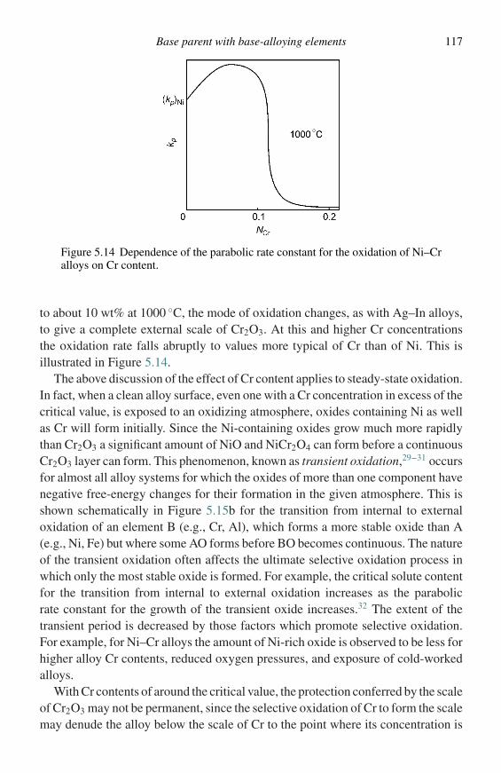
Base parent with base-alloying elements 117
Figure 5.14 Dependence of the parabolic rate constant for the oxidation of Ni–Cralloys on Cr content.
to about 10 wt% at 1000 ◦C, the mode of oxidation changes, as with Ag–In alloys,to give a complete external scale of Cr2O3. At this and higher Cr concentrationsthe oxidation rate falls abruptly to values more typical of Cr than of Ni. This isillustrated in Figure 5.14.
The above discussion of the effect of Cr content applies to steady-state oxidation.In fact, when a clean alloy surface, even one with a Cr concentration in excess of thecritical value, is exposed to an oxidizing atmosphere, oxides containing Ni as wellas Cr will form initially. Since the Ni-containing oxides grow much more rapidlythan Cr2O3 a significant amount of NiO and NiCr2O4 can form before a continuousCr2O3 layer can form. This phenomenon, known as transient oxidation,29–31 occursfor almost all alloy systems for which the oxides of more than one component havenegative free-energy changes for their formation in the given atmosphere. This isshown schematically in Figure 5.15b for the transition from internal to externaloxidation of an element B (e.g., Cr, Al), which forms a more stable oxide than A(e.g., Ni, Fe) but where some AO forms before BO becomes continuous. The natureof the transient oxidation often affects the ultimate selective oxidation process inwhich only the most stable oxide is formed. For example, the critical solute contentfor the transition from internal to external oxidation increases as the parabolicrate constant for the growth of the transient oxide increases.32 The extent of thetransient period is decreased by those factors which promote selective oxidation.For example, for Ni–Cr alloys the amount of Ni-rich oxide is observed to be less forhigher alloy Cr contents, reduced oxygen pressures, and exposure of cold-workedalloys.
With Cr contents of around the critical value, the protection conferred by the scaleof Cr2O3 may not be permanent, since the selective oxidation of Cr to form the scalemay denude the alloy below the scale of Cr to the point where its concentration is
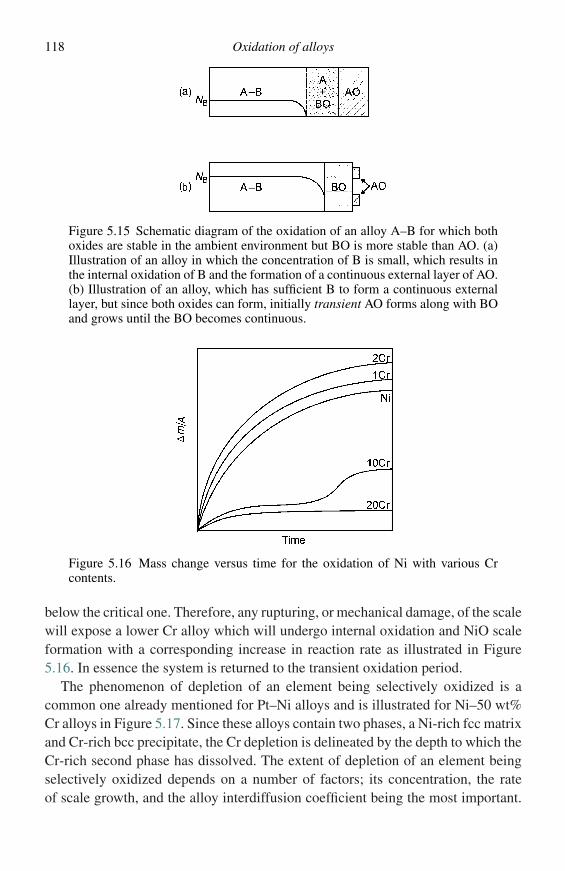
118 Oxidation of alloys
Figure 5.15 Schematic diagram of the oxidation of an alloy A–B for which bothoxides are stable in the ambient environment but BO is more stable than AO. (a)Illustration of an alloy in which the concentration of B is small, which results inthe internal oxidation of B and the formation of a continuous external layer of AO.(b) Illustration of an alloy, which has sufficient B to form a continuous externallayer, but since both oxides can form, initially transient AO forms along with BOand grows until the BO becomes continuous.
Figure 5.16 Mass change versus time for the oxidation of Ni with various Crcontents.
below the critical one. Therefore, any rupturing, or mechanical damage, of the scalewill expose a lower Cr alloy which will undergo internal oxidation and NiO scaleformation with a corresponding increase in reaction rate as illustrated in Figure5.16. In essence the system is returned to the transient oxidation period.
The phenomenon of depletion of an element being selectively oxidized is acommon one already mentioned for Pt–Ni alloys and is illustrated for Ni–50 wt%Cr alloys in Figure 5.17. Since these alloys contain two phases, a Ni-rich fcc matrixand Cr-rich bcc precipitate, the Cr depletion is delineated by the depth to which theCr-rich second phase has dissolved. The extent of depletion of an element beingselectively oxidized depends on a number of factors; its concentration, the rateof scale growth, and the alloy interdiffusion coefficient being the most important.
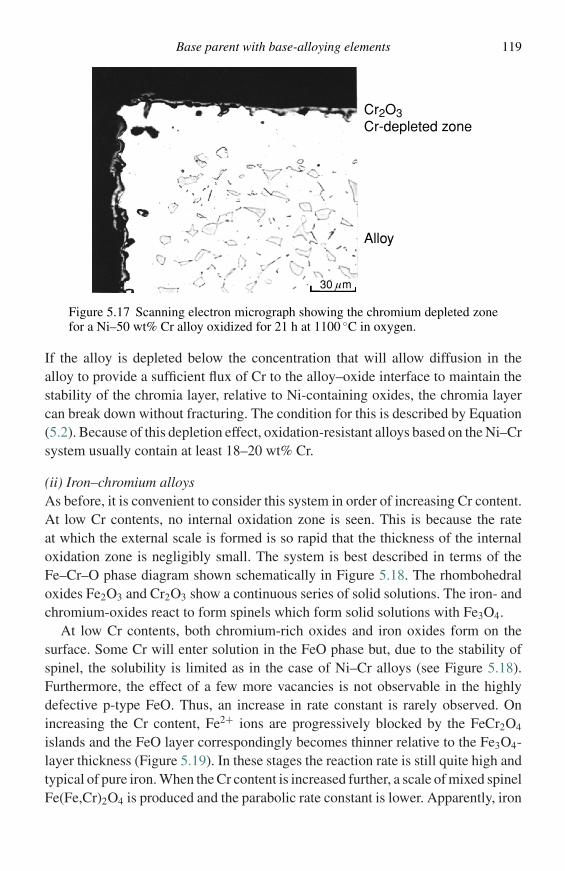
Base parent with base-alloying elements 119
Alloy
Cr2O3Cr-depleted zone
30 µm
Figure 5.17 Scanning electron micrograph showing the chromium depleted zonefor a Ni–50 wt% Cr alloy oxidized for 21 h at 1100 ◦C in oxygen.
If the alloy is depleted below the concentration that will allow diffusion in thealloy to provide a sufficient flux of Cr to the alloy–oxide interface to maintain thestability of the chromia layer, relative to Ni-containing oxides, the chromia layercan break down without fracturing. The condition for this is described by Equation(5.2). Because of this depletion effect, oxidation-resistant alloys based on the Ni–Crsystem usually contain at least 18–20 wt% Cr.
(ii) Iron–chromium alloysAs before, it is convenient to consider this system in order of increasing Cr content.At low Cr contents, no internal oxidation zone is seen. This is because the rateat which the external scale is formed is so rapid that the thickness of the internaloxidation zone is negligibly small. The system is best described in terms of theFe–Cr–O phase diagram shown schematically in Figure 5.18. The rhombohedraloxides Fe2O3 and Cr2O3 show a continuous series of solid solutions. The iron- andchromium-oxides react to form spinels which form solid solutions with Fe3O4.
At low Cr contents, both chromium-rich oxides and iron oxides form on thesurface. Some Cr will enter solution in the FeO phase but, due to the stability ofspinel, the solubility is limited as in the case of Ni–Cr alloys (see Figure 5.18).Furthermore, the effect of a few more vacancies is not observable in the highlydefective p-type FeO. Thus, an increase in rate constant is rarely observed. Onincreasing the Cr content, Fe2+ ions are progressively blocked by the FeCr2O4
islands and the FeO layer correspondingly becomes thinner relative to the Fe3O4-layer thickness (Figure 5.19). In these stages the reaction rate is still quite high andtypical of pure iron. When the Cr content is increased further, a scale of mixed spinelFe(Fe,Cr)2O4 is produced and the parabolic rate constant is lower. Apparently, iron
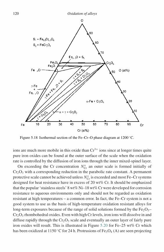
120 Oxidation of alloys
Figure 5.18 Isothermal section of the Fe–Cr–O phase diagram at 1200 ◦C.
ions are much more mobile in this oxide than Cr3+ ions since at longer times quitepure iron oxides can be found at the outer surface of the scale when the oxidationrate is controlled by the diffusion of iron ions through the inner mixed-spinel layer.
On exceeding the Cr concentration N ∗Cr an outer scale is formed initially of
Cr2O3 with a corresponding reduction in the parabolic rate constant. A permanentprotective scale cannot be achieved unless N ∗
Cr is exceeded and most Fe–Cr systemsdesigned for heat resistance have in excess of 20 wt% Cr. It should be emphasizedthat the popular ‘stainless steels’ 8 wt% Ni–18 wt% Cr were developed for corrosionresistance to aqueous environments only and should not be regarded as oxidationresistant at high temperatures – a common error. In fact, the Fe–Cr system is not agood system to use as the basis of high-temperature oxidation resistant alloys forlong-term exposures because of the range of solid solutions formed by the Fe2O3–Cr2O3 rhombohedral oxides. Even with high Cr levels, iron ions will dissolve in anddiffuse rapidly through the Cr2O3 scale and eventually an outer layer of fairly pureiron oxides will result. This is illustrated in Figure 5.20 for Fe–25 wt% Cr whichhas been oxidized at 1150 ◦C for 24 h. Protrusions of Fe3O4 (A) are seen projecting
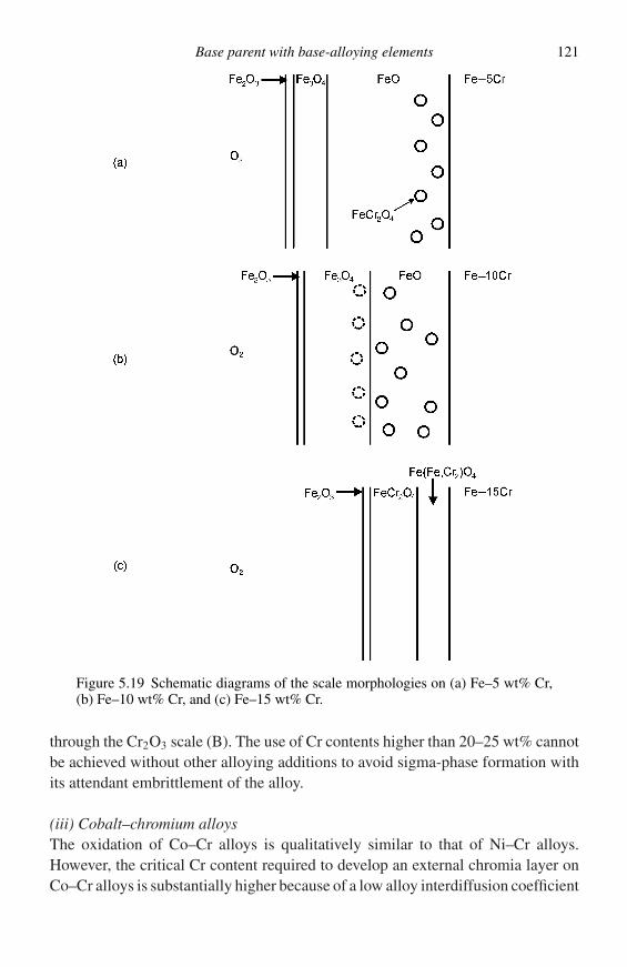
Base parent with base-alloying elements 121
O
Figure 5.19 Schematic diagrams of the scale morphologies on (a) Fe–5 wt% Cr,(b) Fe–10 wt% Cr, and (c) Fe–15 wt% Cr.
through the Cr2O3 scale (B). The use of Cr contents higher than 20–25 wt% cannotbe achieved without other alloying additions to avoid sigma-phase formation withits attendant embrittlement of the alloy.
(iii) Cobalt–chromium alloysThe oxidation of Co–Cr alloys is qualitatively similar to that of Ni–Cr alloys.However, the critical Cr content required to develop an external chromia layer onCo–Cr alloys is substantially higher because of a low alloy interdiffusion coefficient
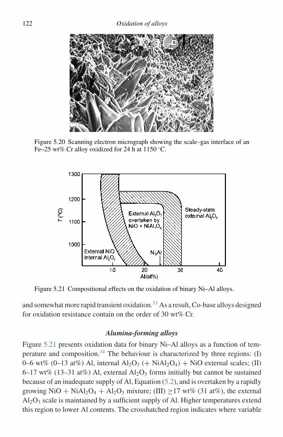
122 Oxidation of alloys
Figure 5.20 Scanning electron micrograph showing the scale–gas interface of anFe–25 wt% Cr alloy oxidized for 24 h at 1150 ◦C.
Figure 5.21 Compositional effects on the oxidation of binary Ni–Al alloys.
and somewhat more rapid transient oxidation.33 As a result, Co-base alloys designedfor oxidation resistance contain on the order of 30 wt% Cr.
Alumina-forming alloys
Figure 5.21 presents oxidation data for binary Ni–Al alloys as a function of tem-perature and composition.34 The behaviour is characterized by three regions: (I)0–6 wt% (0–13 at%) Al, internal Al2O3 (+ NiAl2O4) + NiO external scales; (II)6–17 wt% (13–31 at%) Al, external Al2O3 forms initially but cannot be sustainedbecause of an inadequate supply of Al, Equation (5.2), and is overtaken by a rapidlygrowing NiO + NiAl2O4 + Al2O3 mixture; (III) ≥17 wt% (31 at%), the externalAl2O3 scale is maintained by a sufficient supply of Al. Higher temperatures extendthis region to lower Al contents. The crosshatched region indicates where variable
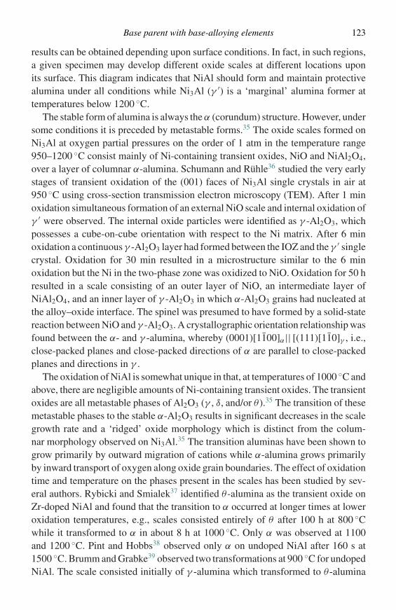
Base parent with base-alloying elements 123
results can be obtained depending upon surface conditions. In fact, in such regions,a given specimen may develop different oxide scales at different locations uponits surface. This diagram indicates that NiAl should form and maintain protectivealumina under all conditions while Ni3Al (γ ′) is a ‘marginal’ alumina former attemperatures below 1200 ◦C.
The stable form of alumina is always the α (corundum) structure. However, undersome conditions it is preceded by metastable forms.35 The oxide scales formed onNi3Al at oxygen partial pressures on the order of 1 atm in the temperature range950–1200 ◦C consist mainly of Ni-containing transient oxides, NiO and NiAl2O4,over a layer of columnar α-alumina. Schumann and Ruhle36 studied the very earlystages of transient oxidation of the (001) faces of Ni3Al single crystals in air at950 ◦C using cross-section transmission electron microscopy (TEM). After 1 minoxidation simultaneous formation of an external NiO scale and internal oxidation ofγ ′ were observed. The internal oxide particles were identified as γ -Al2O3, whichpossesses a cube-on-cube orientation with respect to the Ni matrix. After 6 minoxidation a continuous γ -Al2O3 layer had formed between the IOZ and the γ ′ singlecrystal. Oxidation for 30 min resulted in a microstructure similar to the 6 minoxidation but the Ni in the two-phase zone was oxidized to NiO. Oxidation for 50 hresulted in a scale consisting of an outer layer of NiO, an intermediate layer ofNiAl2O4, and an inner layer of γ -Al2O3 in which α-Al2O3 grains had nucleated atthe alloy–oxide interface. The spinel was presumed to have formed by a solid-statereaction between NiO and γ -Al2O3. A crystallographic orientation relationship wasfound between the α- and γ -alumina, whereby (0001)[1100]α|| [(111)[110]γ , i.e.,close-packed planes and close-packed directions of α are parallel to close-packedplanes and directions in γ .
The oxidation of NiAl is somewhat unique in that, at temperatures of 1000 ◦C andabove, there are negligible amounts of Ni-containing transient oxides. The transientoxides are all metastable phases of Al2O3 (γ , δ, and/or θ ).35 The transition of thesemetastable phases to the stable α-Al2O3 results in significant decreases in the scalegrowth rate and a ‘ridged’ oxide morphology which is distinct from the colum-nar morphology observed on Ni3Al.35 The transition aluminas have been shown togrow primarily by outward migration of cations while α-alumina grows primarilyby inward transport of oxygen along oxide grain boundaries. The effect of oxidationtime and temperature on the phases present in the scales has been studied by sev-eral authors. Rybicki and Smialek37 identified θ -alumina as the transient oxide onZr-doped NiAl and found that the transition to α occurred at longer times at loweroxidation temperatures, e.g., scales consisted entirely of θ after 100 h at 800 ◦Cwhile it transformed to α in about 8 h at 1000 ◦C. Only α was observed at 1100and 1200 ◦C. Pint and Hobbs38 observed only α on undoped NiAl after 160 s at1500 ◦C. Brumm and Grabke39 observed two transformations at 900 ◦C for undopedNiAl. The scale consisted initially of γ -alumina which transformed to θ -alumina
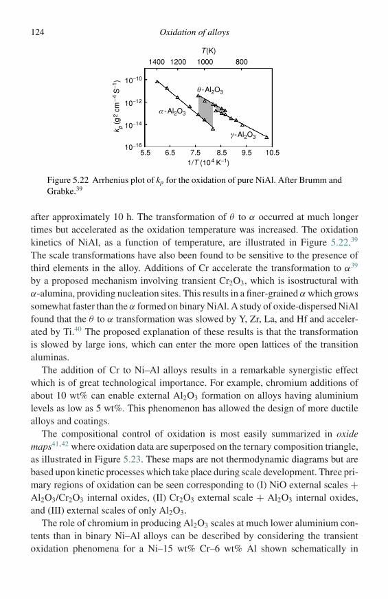
124 Oxidation of alloys
k p (g
2 cm
−4 S
−1) 10−10
10−12
10−14
10−16
5.5 6.5
1400 1200 1000 800
T(K)
7.5
α -Al2O3
γ-Al2O3
8.5 9.51/T (104 K−1)
10.5
θ -Al2O3
Figure 5.22 Arrhenius plot of kp for the oxidation of pure NiAl. After Brumm andGrabke.39
after approximately 10 h. The transformation of θ to α occurred at much longertimes but accelerated as the oxidation temperature was increased. The oxidationkinetics of NiAl, as a function of temperature, are illustrated in Figure 5.22.39
The scale transformations have also been found to be sensitive to the presence ofthird elements in the alloy. Additions of Cr accelerate the transformation to α39
by a proposed mechanism involving transient Cr2O3, which is isostructural withα-alumina, providing nucleation sites. This results in a finer-grained α which growssomewhat faster than the α formed on binary NiAl. A study of oxide-dispersed NiAlfound that the θ to α transformation was slowed by Y, Zr, La, and Hf and acceler-ated by Ti.40 The proposed explanation of these results is that the transformationis slowed by large ions, which can enter the more open lattices of the transitionaluminas.
The addition of Cr to Ni–Al alloys results in a remarkable synergistic effectwhich is of great technological importance. For example, chromium additions ofabout 10 wt% can enable external Al2O3 formation on alloys having aluminiumlevels as low as 5 wt%. This phenomenon has allowed the design of more ductilealloys and coatings.
The compositional control of oxidation is most easily summarized in oxidemaps41,42 where oxidation data are superposed on the ternary composition triangle,as illustrated in Figure 5.23. These maps are not thermodynamic diagrams but arebased upon kinetic processes which take place during scale development. Three pri-mary regions of oxidation can be seen corresponding to (I) NiO external scales +Al2O3/Cr2O3 internal oxides, (II) Cr2O3 external scale + Al2O3 internal oxides,and (III) external scales of only Al2O3.
The role of chromium in producing Al2O3 scales at much lower aluminium con-tents than in binary Ni–Al alloys can be described by considering the transientoxidation phenomena for a Ni–15 wt% Cr–6 wt% Al shown schematically in
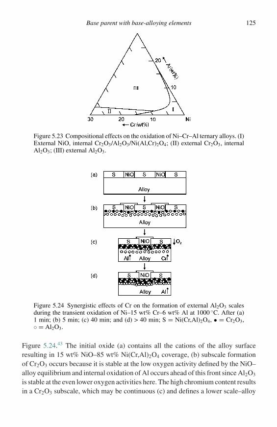
Base parent with base-alloying elements 125
Figure 5.23 Compositional effects on the oxidation of Ni–Cr–Al ternary alloys. (I)External NiO, internal Cr2O3/Al2O3/Ni(Al,Cr)2O4; (II) external Cr2O3, internalAl2O3; (III) external Al2O3.
Figure 5.24 Synergistic effects of Cr on the formation of external Al2O3 scalesduring the transient oxidation of Ni–15 wt% Cr–6 wt% Al at 1000 ◦C. After (a)1 min; (b) 5 min; (c) 40 min; and (d) > 40 min; S = Ni(Cr,Al)2O4, • = Cr2O3,◦ = Al2O3.
Figure 5.24.43 The initial oxide (a) contains all the cations of the alloy surfaceresulting in 15 wt% NiO–85 wt% Ni(Cr,Al)2O4 coverage, (b) subscale formationof Cr2O3 occurs because it is stable at the low oxygen activity defined by the NiO–alloy equilibrium and internal oxidation of Al occurs ahead of this front since Al2O3
is stable at the even lower oxygen activities here. The high chromium content resultsin a Cr2O3 subscale, which may be continuous (c) and defines a lower scale–alloy
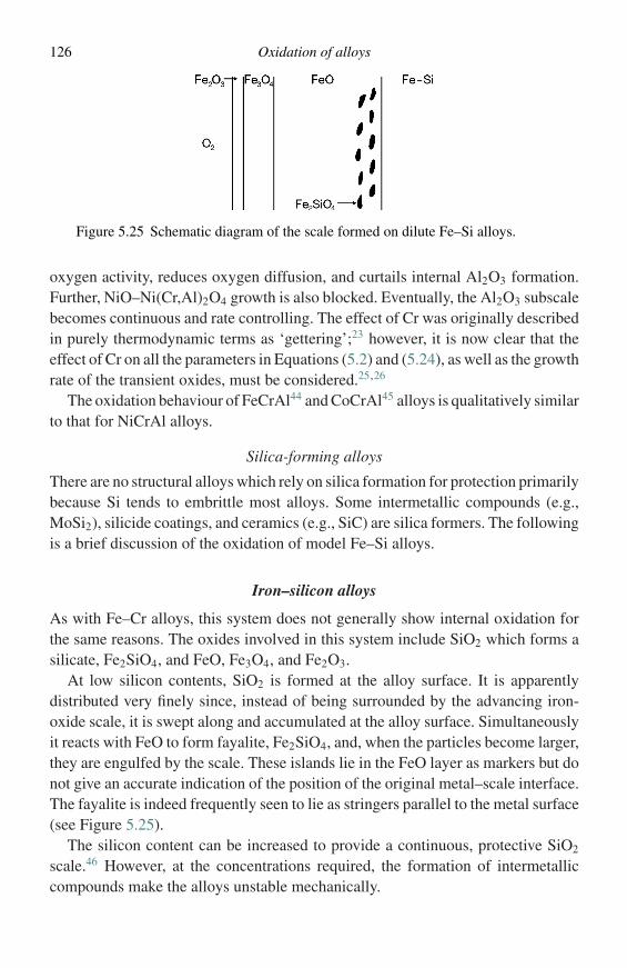
126 Oxidation of alloys
Figure 5.25 Schematic diagram of the scale formed on dilute Fe–Si alloys.
oxygen activity, reduces oxygen diffusion, and curtails internal Al2O3 formation.Further, NiO–Ni(Cr,Al)2O4 growth is also blocked. Eventually, the Al2O3 subscalebecomes continuous and rate controlling. The effect of Cr was originally describedin purely thermodynamic terms as ‘gettering’;23 however, it is now clear that theeffect of Cr on all the parameters in Equations (5.2) and (5.24), as well as the growthrate of the transient oxides, must be considered.25,26
The oxidation behaviour of FeCrAl44 and CoCrAl45 alloys is qualitatively similarto that for NiCrAl alloys.
Silica-forming alloys
There are no structural alloys which rely on silica formation for protection primarilybecause Si tends to embrittle most alloys. Some intermetallic compounds (e.g.,MoSi2), silicide coatings, and ceramics (e.g., SiC) are silica formers. The followingis a brief discussion of the oxidation of model Fe–Si alloys.
Iron–silicon alloys
As with Fe–Cr alloys, this system does not generally show internal oxidation forthe same reasons. The oxides involved in this system include SiO2 which forms asilicate, Fe2SiO4, and FeO, Fe3O4, and Fe2O3.
At low silicon contents, SiO2 is formed at the alloy surface. It is apparentlydistributed very finely since, instead of being surrounded by the advancing iron-oxide scale, it is swept along and accumulated at the alloy surface. Simultaneouslyit reacts with FeO to form fayalite, Fe2SiO4, and, when the particles become larger,they are engulfed by the scale. These islands lie in the FeO layer as markers but donot give an accurate indication of the position of the original metal–scale interface.The fayalite is indeed frequently seen to lie as stringers parallel to the metal surface(see Figure 5.25).
The silicon content can be increased to provide a continuous, protective SiO2
scale.46 However, at the concentrations required, the formation of intermetalliccompounds make the alloys unstable mechanically.
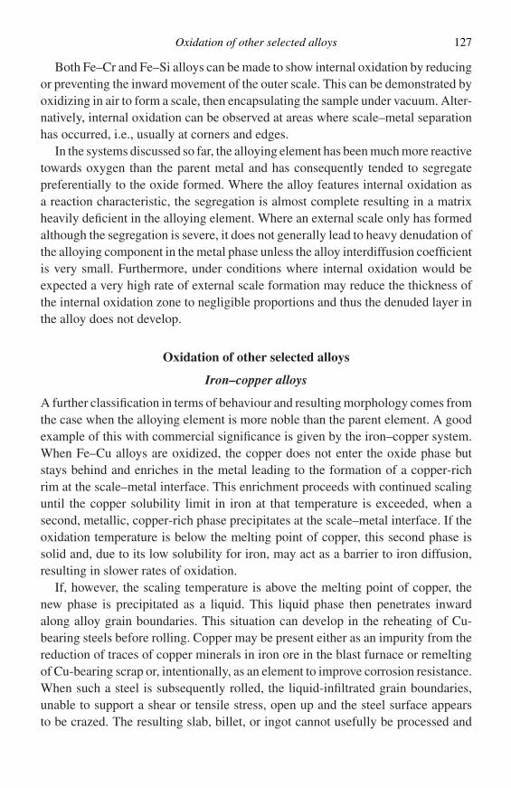
Oxidation of other selected alloys 127
Both Fe–Cr and Fe–Si alloys can be made to show internal oxidation by reducingor preventing the inward movement of the outer scale. This can be demonstrated byoxidizing in air to form a scale, then encapsulating the sample under vacuum. Alter-natively, internal oxidation can be observed at areas where scale–metal separationhas occurred, i.e., usually at corners and edges.
In the systems discussed so far, the alloying element has been much more reactivetowards oxygen than the parent metal and has consequently tended to segregatepreferentially to the oxide formed. Where the alloy features internal oxidation asa reaction characteristic, the segregation is almost complete resulting in a matrixheavily deficient in the alloying element. Where an external scale only has formedalthough the segregation is severe, it does not generally lead to heavy denudation ofthe alloying component in the metal phase unless the alloy interdiffusion coefficientis very small. Furthermore, under conditions where internal oxidation would beexpected a very high rate of external scale formation may reduce the thickness ofthe internal oxidation zone to negligible proportions and thus the denuded layer inthe alloy does not develop.
Oxidation of other selected alloys
Iron–copper alloys
A further classification in terms of behaviour and resulting morphology comes fromthe case when the alloying element is more noble than the parent element. A goodexample of this with commercial significance is given by the iron–copper system.When Fe–Cu alloys are oxidized, the copper does not enter the oxide phase butstays behind and enriches in the metal leading to the formation of a copper-richrim at the scale–metal interface. This enrichment proceeds with continued scalinguntil the copper solubility limit in iron at that temperature is exceeded, when asecond, metallic, copper-rich phase precipitates at the scale–metal interface. If theoxidation temperature is below the melting point of copper, this second phase issolid and, due to its low solubility for iron, may act as a barrier to iron diffusion,resulting in slower rates of oxidation.
If, however, the scaling temperature is above the melting point of copper, thenew phase is precipitated as a liquid. This liquid phase then penetrates inwardalong alloy grain boundaries. This situation can develop in the reheating of Cu-bearing steels before rolling. Copper may be present either as an impurity from thereduction of traces of copper minerals in iron ore in the blast furnace or remeltingof Cu-bearing scrap or, intentionally, as an element to improve corrosion resistance.When such a steel is subsequently rolled, the liquid-infiltrated grain boundaries,unable to support a shear or tensile stress, open up and the steel surface appearsto be crazed. The resulting slab, billet, or ingot cannot usefully be processed and
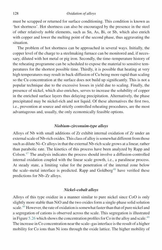
128 Oxidation of alloys
must be scrapped or returned for surface conditioning. This condition is known as‘hot shortness’. Hot shortness can also be encouraged by the presence in the steelof other relatively noble elements, such as Sn, As, Bi, or Sb, which also enrichwith copper and lower the melting point of the second phase, thus aggravating thesituation.
The problem of hot shortness can be approached in several ways. Initially, thecopper level of the charge to a steelmaking furnace can be monitored and, if neces-sary, diluted with hot metal or pig iron. Secondly, the time–temperature history ofthe reheating programme can be scheduled to expose the material to sensitive tem-peratures for the shortest possible time. Thirdly, it is possible that heating at veryhigh temperatures may result in back-diffusion of Cu being more rapid than scalingso the Cu concentration at the surface does not build up significantly. This is not apopular technique due to the excessive losses in yield due to scaling. Finally, thepresence of nickel, which also enriches, serves to increase the solubility of copperin the enriched surface layers thus delaying precipitation. Alternatively, the phaseprecipitated may be nickel-rich and not liquid. Of these alternatives the first two,i.e., prevention at source and strictly controlled reheating procedures, are the mostadvantageous and, usually, the only economically feasible options.
Niobium–zirconuim-type alloys
Alloys of Nb with small additions of Zr exhibit internal oxidation of Zr under anexternal scale of Nb-rich oxides. This class of alloy is somewhat different from thosesuch as dilute Ni–Cr alloys in that the external Nb-rich scale grows at a linear, ratherthan parabolic rate. The kinetics of this process have been analyzed by Rapp andColson.47 The analysis indicates the process should involve a diffusion-controlledinternal oxidation coupled with the linear scale growth, i.e., a paralinear process.At steady state, a limiting value for the penetration of the internal zone belowthe scale–metal interface is predicted. Rapp and Goldberg48 have verified thesepredictions for Nb–Zr alloys.
Nickel–cobalt alloys
Alloys of this type oxidize in a manner similar to pure nickel since CoO is onlyslightly more stable than NiO and the two oxides form a single-phase solid solutionscale.49 However, the rate of oxidation is somewhat faster than that of pure nickel anda segregation of cations is observed across the scale. This segregation is illustratedin Figure 5.26 which shows the concentration profiles for Co in the alloy and scale.49
The increase in Co concentration near the scale–gas interface is the result of a highermobility for Co ions than Ni ions through the oxide lattice. The higher mobility of
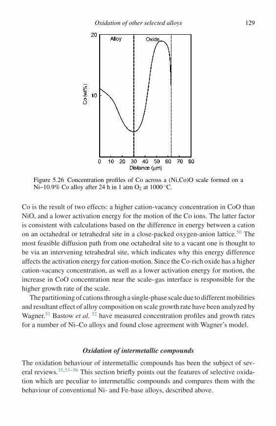
Oxidation of other selected alloys 129
Figure 5.26 Concentration profiles of Co across a (Ni,Co)O scale formed on aNi–10.9% Co alloy after 24 h in 1 atm O2 at 1000 ◦C.
Co is the result of two effects: a higher cation-vacancy concentration in CoO thanNiO, and a lower activation energy for the motion of the Co ions. The latter factoris consistent with calculations based on the difference in energy between a cationon an octahedral or tetrahedral site in a close-packed oxygen-anion lattice.50 Themost feasible diffusion path from one octahedral site to a vacant one is thought tobe via an intervening tetrahedral site, which indicates why this energy differenceaffects the activation energy for cation-motion. Since the Co-rich oxide has a highercation-vacancy concentration, as well as a lower activation energy for motion, theincrease in CoO concentration near the scale–gas interface is responsible for thehigher growth rate of the scale.
The partitioning of cations through a single-phase scale due to different mobilitiesand resultant effect of alloy composition on scale growth rate have been analyzed byWagner.51 Bastow et al. 52 have measured concentration profiles and growth ratesfor a number of Ni–Co alloys and found close agreement with Wagner’s model.
Oxidation of intermetallic compounds
The oxidation behaviour of intermetallic compounds has been the subject of sev-eral reviews.35,53–56 This section briefly points out the features of selective oxida-tion which are peculiar to intermetallic compounds and compares them with thebehaviour of conventional Ni- and Fe-base alloys, described above.
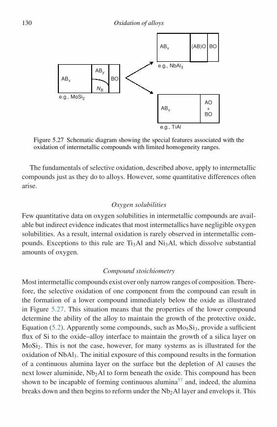
130 Oxidation of alloys
NB
ABy
ABx
ABx
e.g., MoSi2
e.g., NbAl3
e.g., TiAl
BO
(AB)O BO
ABx
AO+
BO
Figure 5.27 Schematic diagram showing the special features associated with theoxidation of intermetallic compounds with limited homogeneity ranges.
The fundamentals of selective oxidation, described above, apply to intermetalliccompounds just as they do to alloys. However, some quantitative differences oftenarise.
Oxygen solubilities
Few quantitative data on oxygen solubilities in intermetallic compounds are avail-able but indirect evidence indicates that most intermetallics have negligible oxygensolubilities. As a result, internal oxidation is rarely observed in intermetallic com-pounds. Exceptions to this rule are Ti3Al and Ni3Al, which dissolve substantialamounts of oxygen.
Compound stoichiometry
Most intermetallic compounds exist over only narrow ranges of composition. There-fore, the selective oxidation of one component from the compound can result inthe formation of a lower compound immediately below the oxide as illustratedin Figure 5.27. This situation means that the properties of the lower compounddetermine the ability of the alloy to maintain the growth of the protective oxide,Equation (5.2). Apparently some compounds, such as Mo5Si3, provide a sufficientflux of Si to the oxide–alloy interface to maintain the growth of a silica layer onMoSi2. This is not the case, however, for many systems as is illustrated for theoxidation of NbAl3. The initial exposure of this compound results in the formationof a continuous alumina layer on the surface but the depletion of Al causes thenext lower aluminide, Nb2Al to form beneath the oxide. This compound has beenshown to be incapable of forming continuous alumina57 and, indeed, the aluminabreaks down and then begins to reform under the Nb2Al layer and envelops it. This
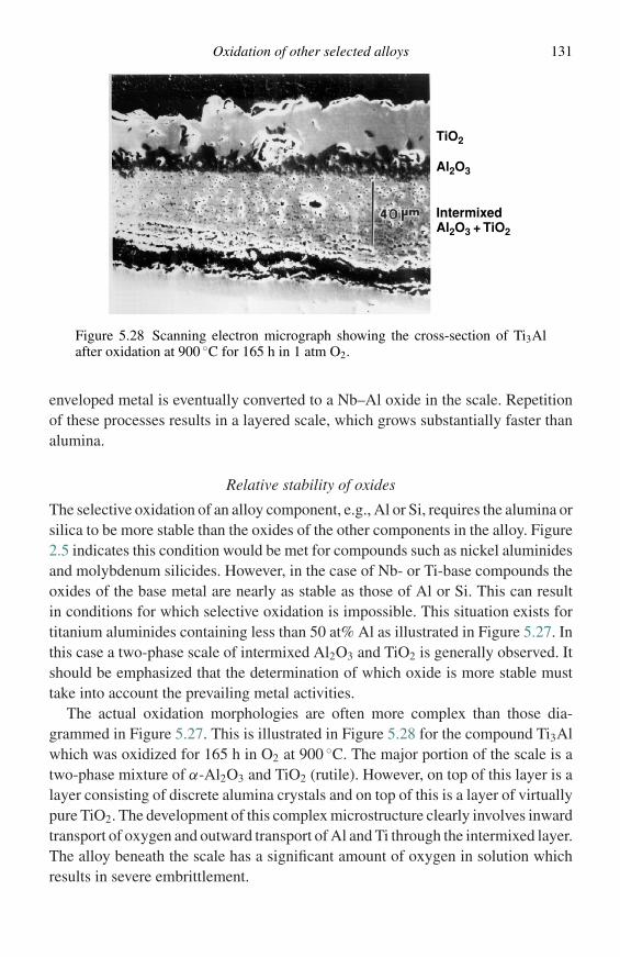
Oxidation of other selected alloys 131
TiO2
Al2O3
IntermixedAl2O3 + TiO2
Figure 5.28 Scanning electron micrograph showing the cross-section of Ti3Alafter oxidation at 900 ◦C for 165 h in 1 atm O2.
enveloped metal is eventually converted to a Nb–Al oxide in the scale. Repetitionof these processes results in a layered scale, which grows substantially faster thanalumina.
Relative stability of oxides
The selective oxidation of an alloy component, e.g., Al or Si, requires the alumina orsilica to be more stable than the oxides of the other components in the alloy. Figure2.5 indicates this condition would be met for compounds such as nickel aluminidesand molybdenum silicides. However, in the case of Nb- or Ti-base compounds theoxides of the base metal are nearly as stable as those of Al or Si. This can resultin conditions for which selective oxidation is impossible. This situation exists fortitanium aluminides containing less than 50 at% Al as illustrated in Figure 5.27. Inthis case a two-phase scale of intermixed Al2O3 and TiO2 is generally observed. Itshould be emphasized that the determination of which oxide is more stable musttake into account the prevailing metal activities.
The actual oxidation morphologies are often more complex than those dia-grammed in Figure 5.27. This is illustrated in Figure 5.28 for the compound Ti3Alwhich was oxidized for 165 h in O2 at 900 ◦C. The major portion of the scale is atwo-phase mixture of α-Al2O3 and TiO2 (rutile). However, on top of this layer is alayer consisting of discrete alumina crystals and on top of this is a layer of virtuallypure TiO2. The development of this complex microstructure clearly involves inwardtransport of oxygen and outward transport of Al and Ti through the intermixed layer.The alloy beneath the scale has a significant amount of oxygen in solution whichresults in severe embrittlement.
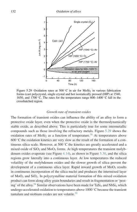
132 Oxidation of alloys
Single crystal (O2)
HIP (1650 °C)-O2
HIP (1540 °C)-Air
HIP (1700 °C)-Air
160120
Oxidation data for 600–1400°Cin air and oxygen
80
Time (h)
400
−1
0
1
2
3
4
5
6
7
∆m/A
(m
g cm
−2)
Cast–(air)
Figure 5.29 Oxidation rates at 500 ◦C in air for MoSi2 in various fabricationforms (cast polycrystal, single crystal and hot isostatically pressed (HIP) at 1540,1650, and 1700 ◦C. The rates for the temperature range 600–1400 ◦C fall in thecrosshatched region.
Growth rate of transient oxides
The formation of transient oxides can influence the ability of an alloy to form aprotective oxide layer, even when the protective oxide is the thermodynamicallystable oxide, as described above. This is particularly true for some intermetalliccompounds such as those involving the refractory metals. Figure 5.29 shows theoxidation rates of MoSi2 as a function of temperature.58 At temperatures above600 ◦C the oxidation kinetics are very slow as the result of the formation of a con-tinuous silica scale. However, at 500 ◦C the kinetics are greatly accelerated and amixed oxide of SiO2 and MoO3 forms. At high temperatures the transient molyb-denum oxides evaporate (see Figure 4.14), as shown in Figure 5.30, and the silicaregions grow laterally into a continuous layer. At low temperatures the reducedvolatility of the molybdenum oxides and the slower growth of silica prevent thedevelopment of a continuous silica layer. Rapid inward growth of MoO3 resultsin continuous incorporation of the silica nuclei and produces the intermixed layerof MoO3 and SiO2. In polycrystalline material formation of this mixed oxidationproduct can form along alloy grain boundaries and result in fragmentation or ‘pest-ing’ of the alloy.58 Similar observations have been made for TaSi2 and NbSi2 whichundergo accelerated oxidation to temperatures above 1000 ◦C because the transienttantalum and niobium oxides are not volatile.59
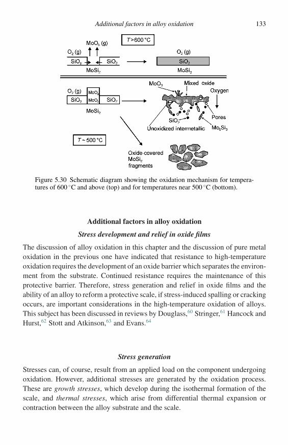
Additional factors in alloy oxidation 133
Figure 5.30 Schematic diagram showing the oxidation mechanism for tempera-tures of 600 ◦C and above (top) and for temperatures near 500 ◦C (bottom).
Additional factors in alloy oxidation
Stress development and relief in oxide films
The discussion of alloy oxidation in this chapter and the discussion of pure metaloxidation in the previous one have indicated that resistance to high-temperatureoxidation requires the development of an oxide barrier which separates the environ-ment from the substrate. Continued resistance requires the maintenance of thisprotective barrier. Therefore, stress generation and relief in oxide films and theability of an alloy to reform a protective scale, if stress-induced spalling or crackingoccurs, are important considerations in the high-temperature oxidation of alloys.This subject has been discussed in reviews by Douglass,60 Stringer,61 Hancock andHurst,62 Stott and Atkinson,63 and Evans.64
Stress generation
Stresses can, of course, result from an applied load on the component undergoingoxidation. However, additional stresses are generated by the oxidation process.These are growth stresses, which develop during the isothermal formation of thescale, and thermal stresses, which arise from differential thermal expansion orcontraction between the alloy substrate and the scale.
134 Oxidation of alloys
Growth stresses
Growth stresses may occur from a number of causes. The proposed mechanismsinclude the following
(1) Volume differences between the oxide and the metal from which it forms.(2) Epitaxial stresses.(3) Compositional changes in the alloy or scale.(4) Point defect stresses.(5) Recrystallization stresses.(6) Oxide formation within the scale.(7) Specimen geometry.
Each of these mechanisms will be discussed individually.
(a) Volume differences between the oxide and the metal
The cause of stress in this case is the fact that the specific volume of the oxide israrely the same as that of the metal which is consumed in its formation. The signof the stress in the oxide may be related to the Pilling–Bedworth ratio (PBR):65
PBR = Vox
Vm. (5.26)
Table 5.1 lists the PBRs for a number of systems.62 The oxide is expected to be incompression if the PBR is greater than unity (which is the case for most metals)
Table 5.1 Oxide–metal-volume ratios of somecommon metals
Oxide Oxide–metal-volume ratio
K2O 0.45MgO 0.81Na2O 0.97Al2O3 1.28ThO2 1.30ZrO2 1.56Cu2O 1.64NiO 1.65FeO (on α-Fe) 1.68TiO2 1.70–1.78CoO 1.86Cr2O3 2.07Fe3O4 (on α-Fe) 2.10Fe2O3 (on α-Fe) 2.14Ta2O5 2.50Nb2O5 2.68V2O5 3.19WO3 3.30
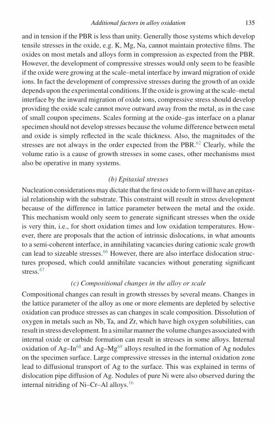
Additional factors in alloy oxidation 135
and in tension if the PBR is less than unity. Generally those systems which developtensile stresses in the oxide, e.g. K, Mg, Na, cannot maintain protective films. Theoxides on most metals and alloys form in compression as expected from the PBR.However, the development of compressive stresses would only seem to be feasibleif the oxide were growing at the scale–metal interface by inward migration of oxideions. In fact the development of compressive stresses during the growth of an oxidedepends upon the experimental conditions. If the oxide is growing at the scale–metalinterface by the inward migration of oxide ions, compressive stress should developproviding the oxide scale cannot move outward away from the metal, as in the caseof small coupon specimens. Scales forming at the oxide–gas interface on a planarspecimen should not develop stresses because the volume difference between metaland oxide is simply reflected in the scale thickness. Also, the magnitudes of thestresses are not always in the order expected from the PBR.62 Clearly, while thevolume ratio is a cause of growth stresses in some cases, other mechanisms mustalso be operative in many systems.
(b) Epitaxial stresses
Nucleation considerations may dictate that the first oxide to form will have an epitax-ial relationship with the substrate. This constraint will result in stress developmentbecause of the difference in lattice parameter between the metal and the oxide.This mechanism would only seem to generate significant stresses when the oxideis very thin, i.e., for short oxidation times and low oxidation temperatures. How-ever, there are proposals that the action of intrinsic dislocations, in what amountsto a semi-coherent interface, in annihilating vacancies during cationic scale growthcan lead to sizeable stresses.66 However, there are also interface dislocation struc-tures proposed, which could annihilate vacancies without generating significantstress.67
(c) Compositional changes in the alloy or scale
Compositional changes can result in growth stresses by several means. Changes inthe lattice parameter of the alloy as one or more elements are depleted by selectiveoxidation can produce stresses as can changes in scale composition. Dissolution ofoxygen in metals such as Nb, Ta, and Zr, which have high oxygen solubilities, canresult in stress development. In a similar manner the volume changes associated withinternal oxide or carbide formation can result in stresses in some alloys. Internaloxidation of Ag–In68 and Ag–Mg69 alloys resulted in the formation of Ag noduleson the specimen surface. Large compressive stresses in the internal oxidation zonelead to diffusional transport of Ag to the surface. This was explained in terms ofdislocation pipe diffusion of Ag. Nodules of pure Ni were also observed during theinternal nitriding of Ni–Cr–Al alloys.16
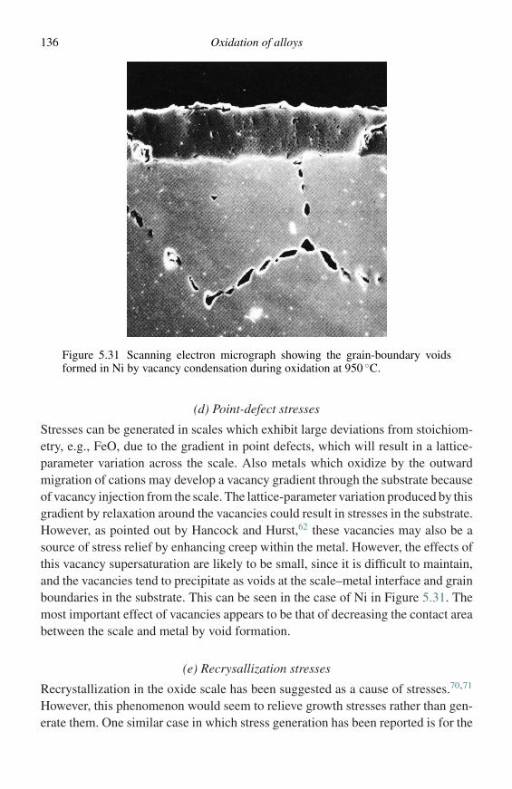
136 Oxidation of alloys
Figure 5.31 Scanning electron micrograph showing the grain-boundary voidsformed in Ni by vacancy condensation during oxidation at 950 ◦C.
(d) Point-defect stresses
Stresses can be generated in scales which exhibit large deviations from stoichiom-etry, e.g., FeO, due to the gradient in point defects, which will result in a lattice-parameter variation across the scale. Also metals which oxidize by the outwardmigration of cations may develop a vacancy gradient through the substrate becauseof vacancy injection from the scale. The lattice-parameter variation produced by thisgradient by relaxation around the vacancies could result in stresses in the substrate.However, as pointed out by Hancock and Hurst,62 these vacancies may also be asource of stress relief by enhancing creep within the metal. However, the effects ofthis vacancy supersaturation are likely to be small, since it is difficult to maintain,and the vacancies tend to precipitate as voids at the scale–metal interface and grainboundaries in the substrate. This can be seen in the case of Ni in Figure 5.31. Themost important effect of vacancies appears to be that of decreasing the contact areabetween the scale and metal by void formation.
(e) Recrysallization stresses
Recrystallization in the oxide scale has been suggested as a cause of stresses.70,71
However, this phenomenon would seem to relieve growth stresses rather than gen-erate them. One similar case in which stress generation has been reported is for the
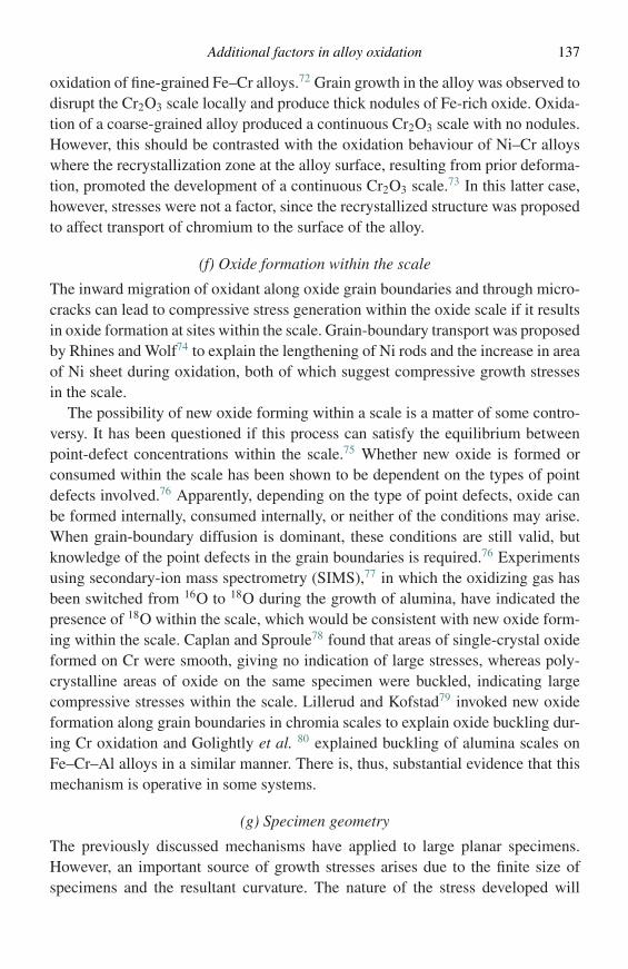
Additional factors in alloy oxidation 137
oxidation of fine-grained Fe–Cr alloys.72 Grain growth in the alloy was observed todisrupt the Cr2O3 scale locally and produce thick nodules of Fe-rich oxide. Oxida-tion of a coarse-grained alloy produced a continuous Cr2O3 scale with no nodules.However, this should be contrasted with the oxidation behaviour of Ni–Cr alloyswhere the recrystallization zone at the alloy surface, resulting from prior deforma-tion, promoted the development of a continuous Cr2O3 scale.73 In this latter case,however, stresses were not a factor, since the recrystallized structure was proposedto affect transport of chromium to the surface of the alloy.
(f) Oxide formation within the scale
The inward migration of oxidant along oxide grain boundaries and through micro-cracks can lead to compressive stress generation within the oxide scale if it resultsin oxide formation at sites within the scale. Grain-boundary transport was proposedby Rhines and Wolf74 to explain the lengthening of Ni rods and the increase in areaof Ni sheet during oxidation, both of which suggest compressive growth stressesin the scale.
The possibility of new oxide forming within a scale is a matter of some contro-versy. It has been questioned if this process can satisfy the equilibrium betweenpoint-defect concentrations within the scale.75 Whether new oxide is formed orconsumed within the scale has been shown to be dependent on the types of pointdefects involved.76 Apparently, depending on the type of point defects, oxide canbe formed internally, consumed internally, or neither of the conditions may arise.When grain-boundary diffusion is dominant, these conditions are still valid, butknowledge of the point defects in the grain boundaries is required.76 Experimentsusing secondary-ion mass spectrometry (SIMS),77 in which the oxidizing gas hasbeen switched from 16O to 18O during the growth of alumina, have indicated thepresence of 18O within the scale, which would be consistent with new oxide form-ing within the scale. Caplan and Sproule78 found that areas of single-crystal oxideformed on Cr were smooth, giving no indication of large stresses, whereas poly-crystalline areas of oxide on the same specimen were buckled, indicating largecompressive stresses within the scale. Lillerud and Kofstad79 invoked new oxideformation along grain boundaries in chromia scales to explain oxide buckling dur-ing Cr oxidation and Golightly et al. 80 explained buckling of alumina scales onFe–Cr–Al alloys in a similar manner. There is, thus, substantial evidence that thismechanism is operative in some systems.
(g) Specimen geometry
The previously discussed mechanisms have applied to large planar specimens.However, an important source of growth stresses arises due to the finite size ofspecimens and the resultant curvature. The nature of the stress developed will
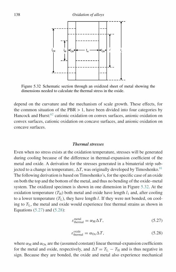
138 Oxidation of alloys
lOX tOX tOXtm l1llM
Figure 5.32 Schematic section through an oxidized sheet of metal showing thedimensions needed to calculate the thermal stress in the oxide.
depend on the curvature and the mechanism of scale growth. These effects, forthe common situation of the PBR > 1, have been divided into four categories byHancock and Hurst:62 cationic oxidation on convex surfaces, anionic oxidation onconvex surfaces, cationic oxidation on concave surfaces, and anionic oxidation onconcave surfaces.
Thermal stresses
Even when no stress exists at the oxidation temperature, stresses will be generatedduring cooling because of the difference in thermal-expansion coefficient of themetal and oxide. A derivation for the stresses generated in a bimaterial strip sub-jected to a change in temperature, �T, was originally developed by Timoshenko.81
The following derivation is based on Timoshenko’s, for the specific case of an oxideon both the top and the bottom of the metal, and thus no bending of the oxide–metalsystem. The oxidized specimen is shown in one dimension in Figure 5.32. At theoxidation temperature (TH) both metal and oxide have length l1 and, after coolingto a lower temperature (TL), they have length l. If they were not bonded, on cool-ing to TL, the metal and oxide would experience free thermal strains as shown inEquations (5.27) and (5.28):
εmetalthermal = αM�T, (5.27)
εoxidethermal = αOx�T, (5.28)
where αM and αOx are the (assumed constant) linear thermal-expansion coefficientsfor the metal and oxide, respectively, and �T = TL − TH and is thus negative insign. Because they are bonded, the oxide and metal also experience mechanical
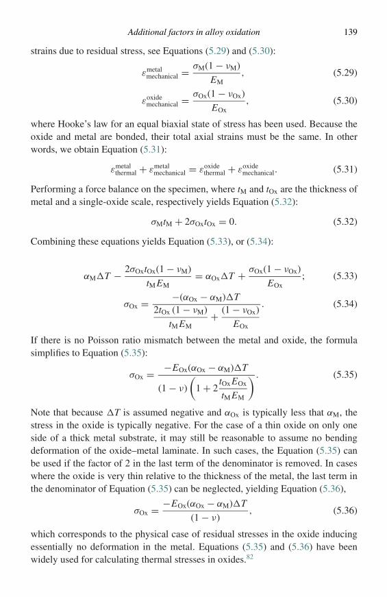
Additional factors in alloy oxidation 139
strains due to residual stress, see Equations (5.29) and (5.30):
εmetalmechanical = σM(1 − νM)
EM, (5.29)
εoxidemechanical = σOx(1 − νOx)
EOx, (5.30)
where Hooke’s law for an equal biaxial state of stress has been used. Because theoxide and metal are bonded, their total axial strains must be the same. In otherwords, we obtain Equation (5.31):
εmetalthermal + εmetal
mechanical = εoxidethermal + εoxide
mechanical. (5.31)
Performing a force balance on the specimen, where tM and tOx are the thickness ofmetal and a single-oxide scale, respectively yields Equation (5.32):
σMtM + 2σOxtOx = 0. (5.32)
Combining these equations yields Equation (5.33), or (5.34):
αM�T − 2σOxtOx(1 − νM)
tM EM= αOx�T + σOx(1 − νOx)
EOx; (5.33)
σOx = −(αOx − αM)�T2tOx (1 − νM)
tM EM+ (1 − νOx)
EOx
. (5.34)
If there is no Poisson ratio mismatch between the metal and oxide, the formulasimplifies to Equation (5.35):
σOx = −EOx(αOx − αM)�T
(1 − ν)
(1 + 2
tOx EOx
tM EM
) . (5.35)
Note that because �T is assumed negative and αOx is typically less that αM, thestress in the oxide is typically negative. For the case of a thin oxide on only oneside of a thick metal substrate, it may still be reasonable to assume no bendingdeformation of the oxide–metal laminate. In such cases, the Equation (5.35) canbe used if the factor of 2 in the last term of the denominator is removed. In caseswhere the oxide is very thin relative to the thickness of the metal, the last term inthe denominator of Equation (5.35) can be neglected, yielding Equation (5.36),
σOx = −EOx(αOx − αM)�T
(1 − ν), (5.36)
which corresponds to the physical case of residual stresses in the oxide inducingessentially no deformation in the metal. Equations (5.35) and (5.36) have beenwidely used for calculating thermal stresses in oxides.82
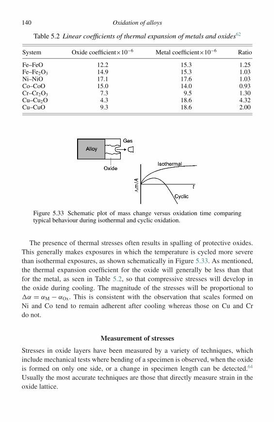
140 Oxidation of alloys
Table 5.2 Linear coefficients of thermal expansion of metals and oxides62
System Oxide coefficient×10−6 Metal coefficient×10−6 Ratio
Fe–FeO 12.2 15.3 1.25Fe–Fe2O3 14.9 15.3 1.03Ni–NiO 17.1 17.6 1.03Co–CoO 15.0 14.0 0.93Cr–Cr2O3 7.3 9.5 1.30Cu–Cu2O 4.3 18.6 4.32Cu–CuO 9.3 18.6 2.00
Figure 5.33 Schematic plot of mass change versus oxidation time comparingtypical behaviour during isothermal and cyclic oxidation.
The presence of thermal stresses often results in spalling of protective oxides.This generally makes exposures in which the temperature is cycled more severethan isothermal exposures, as shown schematically in Figure 5.33. As mentioned,the thermal expansion coefficient for the oxide will generally be less than thatfor the metal, as seen in Table 5.2, so that compressive stresses will develop inthe oxide during cooling. The magnitude of the stresses will be proportional to�α = αM − αOx. This is consistent with the observation that scales formed onNi and Co tend to remain adherent after cooling whereas those on Cu and Crdo not.
Measurement of stresses
Stresses in oxide layers have been measured by a variety of techniques, whichinclude mechanical tests where bending of a specimen is observed, when the oxideis formed on only one side, or a change in specimen length can be detected.64
Usually the most accurate techniques are those that directly measure strain in theoxide lattice.
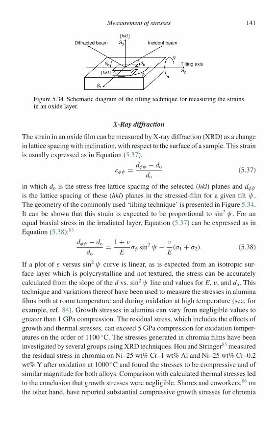
Measurement of stresses 141
φ
ψθbθb
S1
Tilting axisS2
S3
{hkl }
Diffracted beam Incident beam
[hkl ]
Figure 5.34 Schematic diagram of the tilting technique for measuring the strainsin an oxide layer.
X-Ray diffraction
The strain in an oxide film can be measured by X-ray diffraction (XRD) as a changein lattice spacing with inclination, with respect to the surface of a sample. This strainis usually expressed as in Equation (5.37),
εφψ = dφψ − do
do(5.37)
in which do is the stress-free lattice spacing of the selected (hkl) planes and dφψ
is the lattice spacing of these (hkl) planes in the stressed-film for a given tilt ψ .The geometry of the commonly used ‘tilting technique’ is presented in Figure 5.34.It can be shown that this strain is expected to be proportional to sin2 ψ . For anequal biaxial stress in the irradiated layer, Equation (5.37) can be expressed as inEquation (5.38):83
dφψ − do
do= 1 + ν
Eσφ sin2 ψ − ν
E(σ1 + σ2). (5.38)
If a plot of ε versus sin2 ψ curve is linear, as is expected from an isotropic sur-face layer which is polycrystalline and not textured, the stress can be accuratelycalculated from the slope of the d vs. sin2 ψ line and values for E, ν, and do. Thistechnique and variations thereof have been used to measure the stresses in aluminafilms both at room temperature and during oxidation at high temperature (see, forexample, ref. 84). Growth stresses in alumina can vary from negligible values togreater than 1 GPa compression. The residual stress, which includes the effects ofgrowth and thermal stresses, can exceed 5 GPa compression for oxidation temper-atures on the order of 1100 ◦C. The stresses generated in chromia films have beeninvestigated by several groups using XRD techniques. Hou and Stringer85 measuredthe residual stress in chromia on Ni–25 wt% Cr–1 wt% Al and Ni–25 wt% Cr–0.2wt% Y after oxidation at 1000 ◦C and found the stresses to be compressive and ofsimilar magnitude for both alloys. Comparison with calculated thermal stresses ledto the conclusion that growth stresses were negligible. Shores and coworkers,86 onthe other hand, have reported substantial compressive growth stresses for chromia
142 Oxidation of alloys
on Cr. This group has also investigated Ni–Cr alloys and report significant stressrelaxation during the cooling portion of thermal cycles86–88 and growth strains onY-doped alloys which are larger than those on undoped alloys.89
Laser techniques
In some systems it has been shown to be possible to measure strains in oxide films bylaser Raman spectroscopy90 and, in alumina films, by photostimulated chromiumluminescence spectroscopy.91
Response to stress
The growth and thermal stresses generated during oxidation may be accommodatedby a number of mechanisms. The most important are the following:
(1) Cracking of the oxide.(2) Spalling of the oxide from the alloy substrate.(3) Plastic deformation of the substrate.(4) Plastic deformation of the oxide.
All of these mechanisms have been observed to operate in various systems. Theparticular mechanisms will depend in a complicated manner on virtually all of thevariables controlling the oxidation process. Mechanisms (1) and (2) tend to producethe most severe consequences because they can expose fresh metal to the oxidizingenvironment.
Oxide cracking occurs when the oxide is put into tension. This is the situationdescribed for the oxidation of Nb in Chapter 4 which results from the growthmechanism of Nb2O5. Oxides forming on the alkali metals also form under tensionbecause the PBR is less than unity for these systems (Table 5.1).
The oxides on most engineering alloys are in compression because the growthstresses tend to be compressive and, particularly, the thermal stresses, when theydevelop on cooling, are compressive because of the sign of the thermal expansionmismatch between the alloy and oxide (Table 5.2). The spalling of a compressivelystressed protective oxide scale will occur when the elastic strain energy stored inthe intact scale exceeds the fracture resistance, Gc, of the interface. Denoting E andν as the elastic modulus and Poisson’s ratio of the scale, h as the scale thickness,and σ as the equal biaxial residual stress in the film, the elastic strain energy storedin the scale per unit area is (1 − v)σ 2h/E. The criterion for failure then becomesthat given in Equation (5.39):92,93
(1 − ν)σ 2h/E > Gc. (5.39)
Measurement of stresses 143
Gas
GasGas Gas
Alloy Alloy Alloy
Alloy
OxideOxide
Oxide
Oxide
(a) (b) (c)
Figure 5.35 Schematic diagram of responses of an oxide which is loaded in com-pression. (a) Buckling of the oxide, (b) shear cracking of the oxide, and (c) plasticdeformation of the oxide and alloy.
According to this criterion, which is a necessary but not sufficient condition, a scalewill spall if the stress is high, the scale is thick, or the interfacial free energy is high(the work of adhesion is low). Decohesion of films under compression, such asmost oxide scales, however, require either a buckling instability or developmentof a wedge crack in order to spall.64 According to elastic mechanics, buckling ofa thin film under biaxial compression to form an axisymmetric buckle of radius awill occur at a critical stress, σc, given by Equation (5.40):
σc = 1.22E
1 − ν2
(h
a
)2
. (5.40)
However, such a buckle is stable and will not propagate to cause decohesion fail-ure by delamination unless the strain-energy release rate also satisfies Equation(5.39). Figure 5.35(a) shows a schematic diagram of the buckling of a scale andFigures 5.36 and 5.37 show the results of this type of behaviour for alumina scalesformed on Fe–Cr–Al and Fe–Cr–Al–Ti alloys, respectively.
The buckling stress, Equation (5.40), increases as the square of the scale thicknesssuch that, for thick scales, buckling may not be feasible. In this case, shear crackscan form in the oxide and, if Equation (5.39) is satisfied, lead to scale spallation bya ‘wedging mechanism,’ which is shown schematically in Figure 5.35(b).
In some situations, if Gc is high and the alloy is relatively weak, the compressivestresses can be accommodated by simultaneous deformation of the scale and alloywithout spallation. This phenomenon is shown schematically in Figure 5.35(c) andillustrated for an alumina scale in Figure 5.38.
144 Oxidation of alloys
(a)
(b)
Polishingmark
Aluminascale
20 µm
10 µm
Figure 5.36 Scanning electron micrographs of (a) the surface and (b) the cross-section of an Fe–Cr–Al alloy which was oxidized at 1000 ◦C and cooled to roomtemperature. Buckling of the alumina scale is evident.
Reactive element effects
It is now well established that small additions of reactive elements, such as yttrium,hafnium, and cerium, substantially improve the adherence of chromia and aluminafilms to alloy substrates.94 This is illustrated in Figure 5.39 where comparison ofthe cyclic oxidation kinetics of the Fe–Cr–Al (normal S) and Fe–Cr–Al–Y alloysshows the substantial influence of the Y addition. Figure 5.40 shows that the aluminascale on a Fe–Cr–Al–Y alloy is still completely adherent after the exposure. Whilethe effects produced by the reactive elements are widely known, the mechanismswhereby they improve adherence are not completely understood. Over the lastfifty years a number of mechanisms have been proposed. These include: reactiveelements acting as vacancy sinks to suppress void formation at the alloy–oxideinterface,95,96 formation of oxide pegs at the alloy–oxide interface,97 alteration ofthe growth mechanism of the oxide resulting in reduced growth stresses,80 reactive-element segregation to the alloy–oxide interface to form a graded seal98 or otherwise
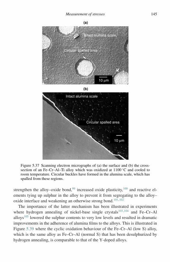
Measurement of stresses 145
(a)
(b)
Intact alumina scale
Intact alumina scale
Circular spalled area
Circular spalled area
10 µm
10 µm
Figure 5.37 Scanning electron micrographs of (a) the surface and (b) the cross-section of an Fe–Cr–Al–Ti alloy which was oxidized at 1100 ◦C and cooled toroom temperature. Circular buckles have formed in the alumina scale, which hasspalled from these regions.
strengthen the alloy–oxide bond,99 increased oxide plasticity,100 and reactive el-ements tying up sulphur in the alloy to prevent it from segregating to the alloy–oxide interface and weakening an otherwise strong bond.101,102
The importance of the latter mechanism has been illustrated in experimentswhere hydrogen annealing of nickel-base single crystals103,104 and Fe–Cr–Alalloys105 lowered the sulphur contents to very low levels and resulted in dramaticimprovements in the adherence of alumina films to the alloys. This is illustrated inFigure 5.39 where the cyclic oxidation behaviour of the Fe–Cr–Al (low S) alloy,which is the same alloy as Fe–Cr–Al (normal S) that has been desulphurized byhydrogen annealing, is comparable to that of the Y-doped alloys.
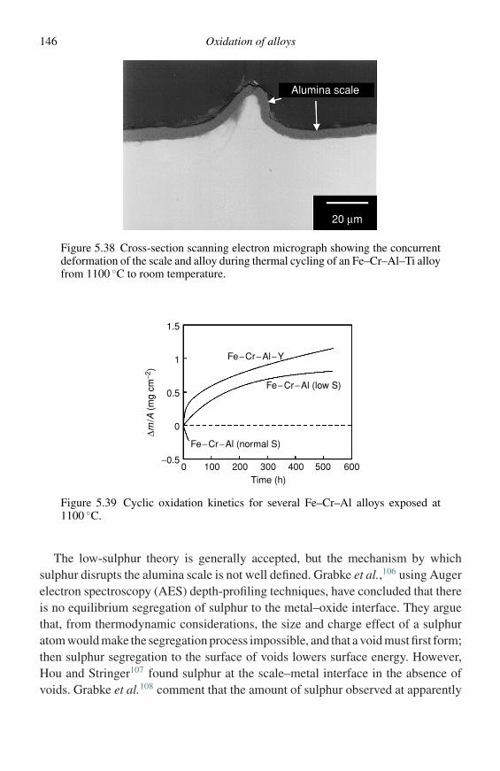
146 Oxidation of alloys
Alumina scale
20 µm
Figure 5.38 Cross-section scanning electron micrograph showing the concurrentdeformation of the scale and alloy during thermal cycling of an Fe–Cr–Al–Ti alloyfrom 1100 ◦C to room temperature.
0 100 200 300 400 500
0
−0.5
1.5
1
0.5
600Time (h)
Fe−Cr−Al (normal S)
Fe−Cr−Al (low S)
Fe−Cr−Al−Y
∆m/A
(m
g cm
−2)
Figure 5.39 Cyclic oxidation kinetics for several Fe–Cr–Al alloys exposed at1100 ◦C.
The low-sulphur theory is generally accepted, but the mechanism by whichsulphur disrupts the alumina scale is not well defined. Grabke et al.,106 using Augerelectron spectroscopy (AES) depth-profiling techniques, have concluded that thereis no equilibrium segregation of sulphur to the metal–oxide interface. They arguethat, from thermodynamic considerations, the size and charge effect of a sulphuratom would make the segregation process impossible, and that a void must first form;then sulphur segregation to the surface of voids lowers surface energy. However,Hou and Stringer107 found sulphur at the scale–metal interface in the absence ofvoids. Grabke et al.108 comment that the amount of sulphur observed at apparently
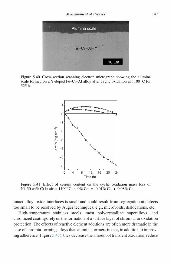
Measurement of stresses 147
Alumina scale
Fe−Cr−Al−Y
10 µm
Figure 5.40 Cross-section scanning electron micrograph showing the aluminascale formed on a Y-doped Fe–Cr–Al alloy after cyclic oxidation at 1100 ◦C for525 h.
Time (h)
−6
−5
−4
−3
−2
−1
0
1
0 4 8 12 16 20 24
∆m
/A (
mg
cm−2
)
Figure 5.41 Effect of cerium content on the cyclic oxidation mass loss ofNi–50 wt% Cr in air at 1100 ◦C: ◦, 0% Ce; �, 0.01% Ce; •, 0.08% Ce.
intact alloy–oxide interfaces is small and could result from segregation at defectstoo small to be resolved by Auger techniques, e.g., microvoids, dislocations, etc.
High-temperature stainless steels, most polycrystalline superalloys, andchromized coatings rely on the formation of a surface layer of chromia for oxidationprotection. The effects of reactive element additions are often more dramatic in thecase of chromia-forming alloys than alumina formers in that, in addition to improv-ing adherence (Figure 5.41), they decrease the amount of transient oxidation, reduce
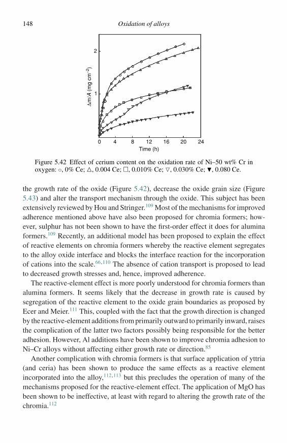
148 Oxidation of alloys
1
2
0 4 8 12 16 20 24Time (h)
∆m/A
(m
g cm
−2)
Figure 5.42 Effect of cerium content on the oxidation rate of Ni–50 wt% Cr inoxygen: ◦, 0% Ce; �, 0.004 Ce; �, 0.010% Ce; �, 0.030% Ce; �, 0.080 Ce.
the growth rate of the oxide (Figure 5.42), decrease the oxide grain size (Figure5.43) and alter the transport mechanism through the oxide. This subject has beenextensively reviewed by Hou and Stringer.109 Most of the mechanisms for improvedadherence mentioned above have also been proposed for chromia formers; how-ever, sulphur has not been shown to have the first-order effect it does for aluminaformers.109 Recently, an additional model has been proposed to explain the effectof reactive elements on chromia formers whereby the reactive element segregatesto the alloy oxide interface and blocks the interface reaction for the incorporationof cations into the scale.66,110 The absence of cation transport is proposed to leadto decreased growth stresses and, hence, improved adherence.
The reactive-element effect is more poorly understood for chromia formers thanalumina formers. It seems likely that the decrease in growth rate is caused bysegregation of the reactive element to the oxide grain boundaries as proposed byEcer and Meier.111 This, coupled with the fact that the growth direction is changedby the reactive-element additions from primarily outward to primarily inward, raisesthe complication of the latter two factors possibly being responsible for the betteradhesion. However, Al additions have been shown to improve chromia adhesion toNi–Cr alloys without affecting either growth rate or direction.85
Another complication with chromia formers is that surface application of yttria(and ceria) has been shown to produce the same effects as a reactive elementincorporated into the alloy,112,113 but this precludes the operation of many of themechanisms proposed for the reactive-element effect. The application of MgO hasbeen shown to be ineffective, at least with regard to altering the growth rate of thechromia.112
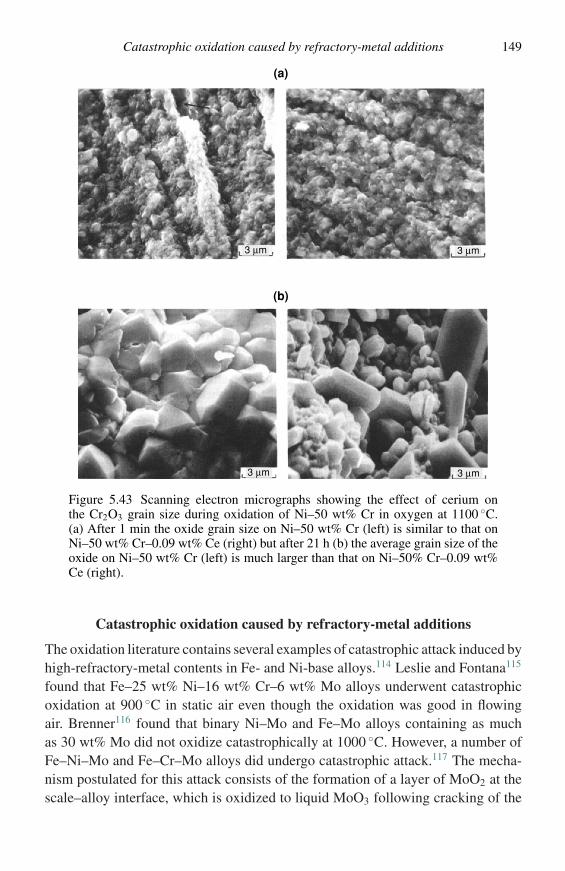
Catastrophic oxidation caused by refractory-metal additions 149
(a)
(b)
3 µm 3 µm
3 µm3 µm
Figure 5.43 Scanning electron micrographs showing the effect of cerium onthe Cr2O3 grain size during oxidation of Ni–50 wt% Cr in oxygen at 1100 ◦C.(a) After 1 min the oxide grain size on Ni–50 wt% Cr (left) is similar to that onNi–50 wt% Cr–0.09 wt% Ce (right) but after 21 h (b) the average grain size of theoxide on Ni–50 wt% Cr (left) is much larger than that on Ni–50% Cr–0.09 wt%Ce (right).
Catastrophic oxidation caused by refractory-metal additions
The oxidation literature contains several examples of catastrophic attack induced byhigh-refractory-metal contents in Fe- and Ni-base alloys.114 Leslie and Fontana115
found that Fe–25 wt% Ni–16 wt% Cr–6 wt% Mo alloys underwent catastrophicoxidation at 900 ◦C in static air even though the oxidation was good in flowingair. Brenner116 found that binary Ni–Mo and Fe–Mo alloys containing as muchas 30 wt% Mo did not oxidize catastrophically at 1000 ◦C. However, a number ofFe–Ni–Mo and Fe–Cr–Mo alloys did undergo catastrophic attack.117 The mecha-nism postulated for this attack consists of the formation of a layer of MoO2 at thescale–alloy interface, which is oxidized to liquid MoO3 following cracking of the
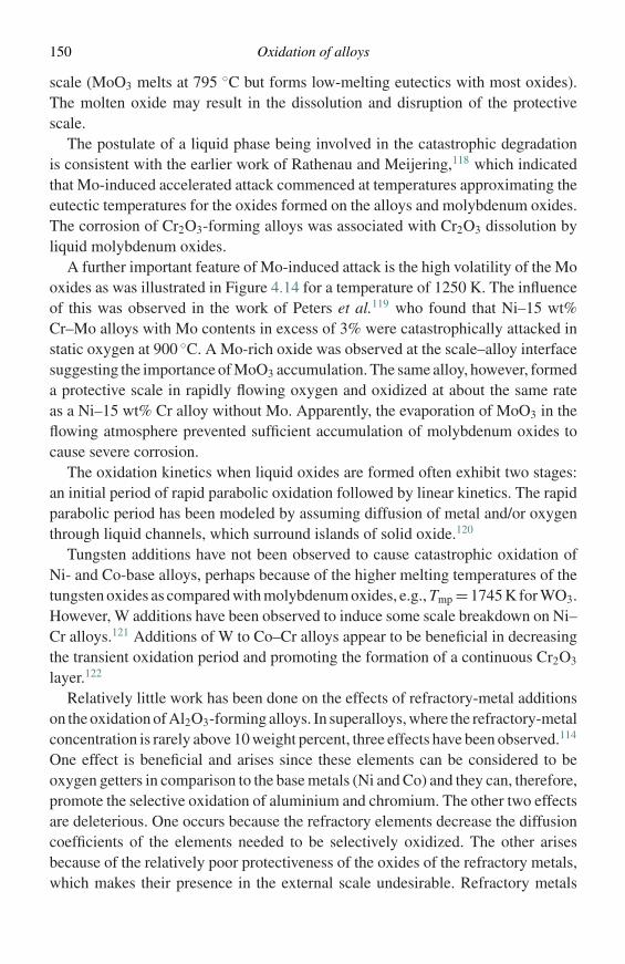
150 Oxidation of alloys
scale (MoO3 melts at 795 ◦C but forms low-melting eutectics with most oxides).The molten oxide may result in the dissolution and disruption of the protectivescale.
The postulate of a liquid phase being involved in the catastrophic degradationis consistent with the earlier work of Rathenau and Meijering,118 which indicatedthat Mo-induced accelerated attack commenced at temperatures approximating theeutectic temperatures for the oxides formed on the alloys and molybdenum oxides.The corrosion of Cr2O3-forming alloys was associated with Cr2O3 dissolution byliquid molybdenum oxides.
A further important feature of Mo-induced attack is the high volatility of the Mooxides as was illustrated in Figure 4.14 for a temperature of 1250 K. The influenceof this was observed in the work of Peters et al.119 who found that Ni–15 wt%Cr–Mo alloys with Mo contents in excess of 3% were catastrophically attacked instatic oxygen at 900 ◦C. A Mo-rich oxide was observed at the scale–alloy interfacesuggesting the importance of MoO3 accumulation. The same alloy, however, formeda protective scale in rapidly flowing oxygen and oxidized at about the same rateas a Ni–15 wt% Cr alloy without Mo. Apparently, the evaporation of MoO3 in theflowing atmosphere prevented sufficient accumulation of molybdenum oxides tocause severe corrosion.
The oxidation kinetics when liquid oxides are formed often exhibit two stages:an initial period of rapid parabolic oxidation followed by linear kinetics. The rapidparabolic period has been modeled by assuming diffusion of metal and/or oxygenthrough liquid channels, which surround islands of solid oxide.120
Tungsten additions have not been observed to cause catastrophic oxidation ofNi- and Co-base alloys, perhaps because of the higher melting temperatures of thetungsten oxides as compared with molybdenum oxides, e.g., Tmp =1745 K for WO3.However, W additions have been observed to induce some scale breakdown on Ni–Cr alloys.121 Additions of W to Co–Cr alloys appear to be beneficial in decreasingthe transient oxidation period and promoting the formation of a continuous Cr2O3
layer.122
Relatively little work has been done on the effects of refractory-metal additionson the oxidation of Al2O3-forming alloys. In superalloys, where the refractory-metalconcentration is rarely above 10 weight percent, three effects have been observed.114
One effect is beneficial and arises since these elements can be considered to beoxygen getters in comparison to the base metals (Ni and Co) and they can, therefore,promote the selective oxidation of aluminium and chromium. The other two effectsare deleterious. One occurs because the refractory elements decrease the diffusioncoefficients of the elements needed to be selectively oxidized. The other arisesbecause of the relatively poor protectiveness of the oxides of the refractory metals,which makes their presence in the external scale undesirable. Refractory metals
Catastrophic oxidation caused by refractory-metal additions 151
have been observed to initiate severe corrosion when a molten sulphate deposit ison the alloy.123 This phenomenon will be discussed in Chapter 8.
Oxidation and decarburization of steels
The oxidation of carbon and low-alloy steels follows oxidation mechanisms similarto those described for the oxidation of pure iron in Chapter 4. At low temperatures(≈ 500 ◦C), typical of service conditions, the alloys form layered scales consistingof Fe3O4 and Fe2O3. The oxidation of Fe–C alloys containing 0.1, 0.5 and 1.0 wt%C at 500 ◦C in 1 atm oxygen has been studied by Caplan et al.124 It was foundthat the oxide scales grew thicker over pearlite colonies than over single-phaseferrite for annealed alloys as the result of a finer grained Fe3O4 layer forming overthe pearlite. Cold-worked alloys oxidized substantially faster than annealed alloys.No carburization or decarburization was observed for any of the alloys. This waspostulated to result from C diffusing out through the inner portion of the Fe3O4
layer and being oxidized to CO which escaped through channels and pores in theouter part of the Fe3O4 and the Fe2O3 layer. Decarburization has been reported at500 ◦C for oxygen partial pressures on the order of 10 torr.125
Oxidation at high temperatures, typical of reheating conditions during steel pro-cessing, can lead to substantial decarburization. This can have a large effect onthe properties of components. The tensile strength of a heat-treated steel dependsprimarily on the carbon content. The maximum stress on a component in bend-ing occurs at the surface. Clearly, if excessive failure of steel components inservice, particularly under reversing bending stresses, is to be avoided, the spec-ified carbon content must be maintained within the surface layers of the compo-nent. This is particularly necessary with rotating shafts and stressed threads inbolts, etc.
Unfortunately, there is a strong tendency for carbon to be lost from the surface ofsteel when it is reheated for hot working or for heat treatment. The loss of carbon,decarburization, is one of the oldest, most persistent problems in ferrous productionmetallurgy.
During normal reheating which is usually carried out in a large furnace wherethe steel stock is in contact with the products of combustion of a fuel (usually oilor gas), the steel oxidizes to form a scale and, therefore, undergoes simultaneousdecarburization and scaling. The mechanisms by which the decarburization of steelsoccurs are well understood,126,127 particularly in the case of plain carbon and low-alloy steels to which the following discussion is confined.
Basically, in the oxidizing atmosphere of the furnace, a scale of iron oxide formsand grows. At the scale–metal interface, carbon interacts with the scale to form
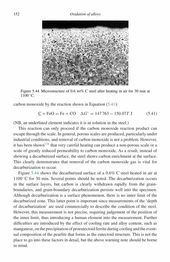
152 Oxidation of alloys
Figure 5.44 Microstructure of 0.6 wt% C steel after heating in air for 30 min at1100 ◦C.
carbon monoxide by the reaction shown in Equation (5.41):
C + FeO = Fe + CO �G◦ = 147 763 − 150.07T J (5.41)
(NB, an underlined element indicates it is in solution in the steel.)This reaction can only proceed if the carbon monoxide reaction product can
escape through the scale. In general, porous scales are produced, particularly underindustrial conditions, and removal of carbon monoxide is not a problem. However,it has been shown128 that very careful heating can produce a non-porous scale or ascale of greatly reduced permeability to carbon monoxide. As a result, instead ofshowing a decarburized surface, the steel shows carbon enrichment at the surface.This clearly demonstrates that removal of the carbon monoxide gas is vital fordecarburization to occur.
Figure 5.44 shows the decarburized surface of a 0.6% C steel heated in air at1100 ◦C for 30 min. Several points should be noted. The decarburization occursin the surface layers, but carbon is clearly withdrawn rapidly from the grain-boundaries, and grain-boundary decarburization persists well into the specimen.Although decarburization is a surface phenomenon, there is no inner limit of thedecarburized zone. This latter point is important since measurements of the ‘depthof decarburization’ are used commercially to describe the condition of the steel.However, this measurement is not precise, requiring judgement of the position ofthe inner limit, thus introducing a human element into the measurement. Furtherdifficulties are introduced by the effect of cooling rate and alloy content, such asmanganese, on the precipitation of proeutectoid ferrite during cooling and the event-ual composition of the pearlite that forms as the eutectoid structure. This is not theplace to go into these factors in detail, but the above warning note should be bornein mind.
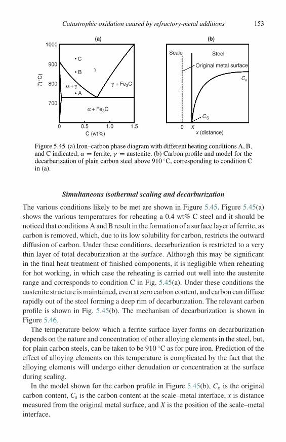
Catastrophic oxidation caused by refractory-metal additions 153
(a) (b)1000
900
800
700
0 0.5 1.0 1.5
T(°
C)
C (wt%)
C
B
Aα + γ γ + Fe3C
α + Fe3C
γ
Scale Steel
Original metal surface
Cο
Cs
x (distance)X0
Figure 5.45 (a) Iron–carbon phase diagram with different heating conditions A, B,and C indicated; α = ferrite, γ = austenite. (b) Carbon profile and model for thedecarburization of plain carbon steel above 910 ◦C, corresponding to condition Cin (a).
Simultaneous isothermal scaling and decarburization
The various conditions likely to be met are shown in Figure 5.45. Figure 5.45(a)shows the various temperatures for reheating a 0.4 wt% C steel and it should benoticed that conditions A and B result in the formation of a surface layer of ferrite, ascarbon is removed, which, due to its low solubility for carbon, restricts the outwarddiffusion of carbon. Under these conditions, decarburization is restricted to a verythin layer of total decaburization at the surface. Although this may be significantin the final heat treatment of finished components, it is negligible when reheatingfor hot working, in which case the reheating is carried out well into the austeniterange and corresponds to condition C in Fig. 5.45(a). Under these conditions theaustenite structure is maintained, even at zero carbon content, and carbon can diffuserapidly out of the steel forming a deep rim of decarburization. The relevant carbonprofile is shown in Fig. 5.45(b). The mechanism of decarburization is shown inFigure 5.46.
The temperature below which a ferrite surface layer forms on decarburizationdepends on the nature and concentration of other alloying elements in the steel, but,for plain carbon steels, can be taken to be 910 ◦C as for pure iron. Prediction of theeffect of alloying elements on this temperature is complicated by the fact that thealloying elements will undergo either denudation or concentration at the surfaceduring scaling.
In the model shown for the carbon profile in Figure 5.45(b), Co is the originalcarbon content, Cs is the carbon content at the scale–metal interface, x is distancemeasured from the original metal surface, and X is the position of the scale–metalinterface.
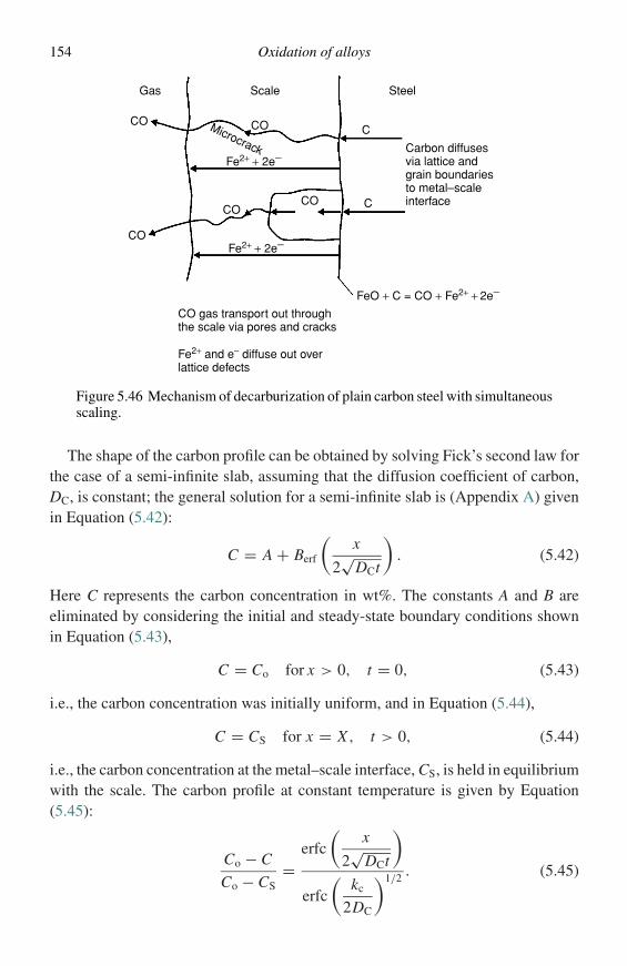
154 Oxidation of alloys
CO
COCO
CO
Gas Scale Steel
C
C
Fe2+ + 2e−
Fe2+ + 2e−
Microcrack Carbon diffusesvia lattice andgrain boundariesto metal–scaleinterface
FeO + C = CO + Fe2+ + 2e−
CO gas transport out throughthe scale via pores and cracks
Fe2+ and e− diffuse out overlattice defects
CO
Figure 5.46 Mechanism of decarburization of plain carbon steel with simultaneousscaling.
The shape of the carbon profile can be obtained by solving Fick’s second law forthe case of a semi-infinite slab, assuming that the diffusion coefficient of carbon,DC, is constant; the general solution for a semi-infinite slab is (Appendix A) givenin Equation (5.42):
C = A + Berf
(x
2√
DCt
). (5.42)
Here C represents the carbon concentration in wt%. The constants A and B areeliminated by considering the initial and steady-state boundary conditions shownin Equation (5.43),
C = Co for x > 0, t = 0, (5.43)
i.e., the carbon concentration was initially uniform, and in Equation (5.44),
C = CS for x = X , t > 0, (5.44)
i.e., the carbon concentration at the metal–scale interface, CS, is held in equilibriumwith the scale. The carbon profile at constant temperature is given by Equation(5.45):
Co − C
Co − CS=
erfc
(x
2√
DCt
)
erfc
(kc
2DC
)1/2 . (5.45)
Catastrophic oxidation caused by refractory-metal additions 155
where kc is the parabolic rate constant for the oxidation of the steel given by Equation(5.46),
kc = X2
2t, (5.46)
where X is the depth of metal consumed by scale formation at time t. Equation(5.45) can be simplified by setting CS = 0, since this value is extremely low(≈0.01 wt%), yielding Equation (5.47):
C = Co
1 −
erfc
(x
2√
DCt
)
erfc
(kc
2DC
)1/2
. (5.47)
Using a steel of 0.85 wt% C, 0.85 wt% Mn, and 0.18 wt% Si, data for kc wereobtained by direct measurement129 and found to obey the relationship shown inEquation (5.48):
kc = 57.1 exp
(−21 720
T
)mm2 s−1. (5.48)
In practice, the value of DC varies with carbon content, but values for low car-bon content were found to give good agreement between calculated and measuredprofiles.128 Extrapolating the data of Wells130 to zero carbon content yielded128
Equation (5.49):
DC = 24.6 exp
(−17 540
T
)mm2 s−1. (5.49)
Combining Equations (5.47), (5.48), and (5.49), carbon profiles can be calculatedand, as shown in Figure 5.47, these give excellent agreement with measured profiles.
The actual value of the depth of decarburization is more difficult to establish sincethe carbon profile is smooth and it is difficult to define an inner limit. Althoughthis could, and perhaps should, be set by defining a carbon content below whichthe mechanical properties of the steel are below specification, current practicerelies on the choice of this position ‘by eye’ by an experienced metallographer. Bycomparing reported depths of decarburization with the carbon profiles, the innerlimit was established as the position where the carbon content is 92% of the originaluniform carbon content of the steel. This is also indicated in Figure 5.47.
Denoting the position of the inner limit as x = x∗, where C = C∗ = 0.92Co, thedepth of decarburization, d, can now be established as shown in Equation (5.50),
d = x∗ − X = x∗ − (2kct)1/2; (5.50)
it can be seen that the value of d depends on the value of X or kc, and in atmosphereswhere scaling is rapid kc and X will be high and d will be correspondingly low.
156 Oxidation of alloys
0
0.2
0.4
0.6
0.8
1.0
0.5 1.0 1.5 2.0 2.5
C(w
t%)
0.92CO
AnalysedPredicted
Inner limit ofdecarburizationzone
Metal–scaleinterface
x –X (mm)
Figure 5.47 Comparison of analyzed and predicted profiles for 0.85 wt% C steelheated at 1100 ◦C for 90 min showing the position of the inner decarburizationlimit.
Equation (5.50) has been evaluated for a eutectoid steel and the depth of decar-burization over the temperature range 900–1300 ◦C has been shown to be given byEquation (5.51)129,131
d = 10.5 exp
(−8710
T
)t1/2 mm (5.51)
where t is in s. Equation (5.51) allows the observed depth of decarburization at aconstant temperature, T, between 900 and 1300 ◦C, to be calculated for a 0.85 wt%C steel. For other steels a similar equation would be valid, the difference beingmainly in the pre-exponential term.
It should also be noted that, in steels of lower carbon content than the eutectoidcomposition, the presence of ferrite in the microstructure makes the judgement ofthe inner limit of decarburization more difficult and open to greater error. Thus, theagreement between prediction and observation is expected to deteriorate at lowercarbon contents.
Effects of scaling rate on decarburization
One of the most common fallacies is to attempt to reduce decarburization by reduc-ing the oxygen potential in the furnace. Since the carbon content at the metal–scaleinterface is constant, so long as FeO remains in contact with the steel, the drivingforce for carbon diffusion is also constant in the presence of a scale. However, byreducing the oxygen potential of the atmosphere, the scaling rate can be reducedand this will affect the observed depth of decarburization.
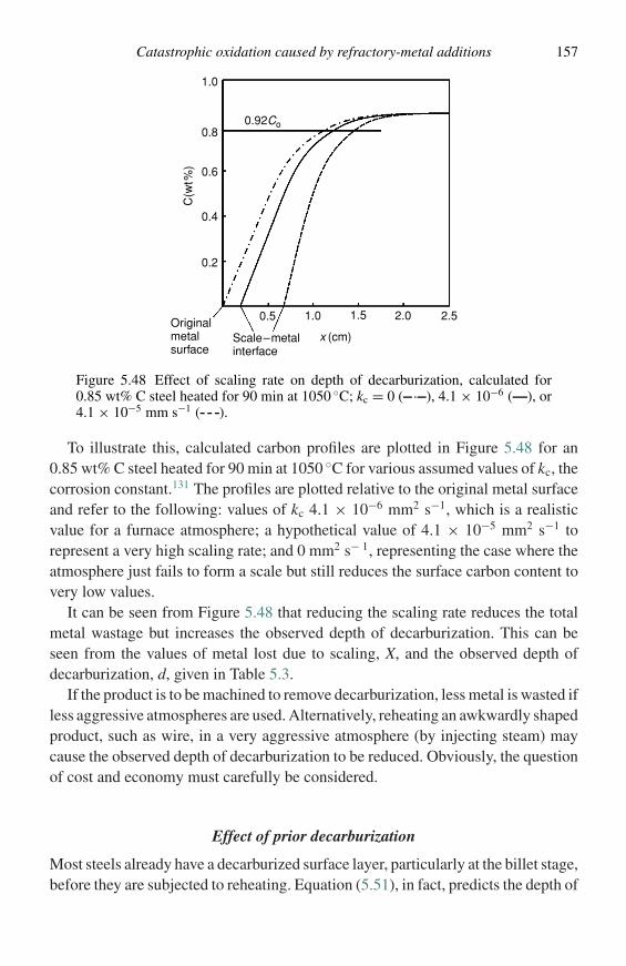
Catastrophic oxidation caused by refractory-metal additions 157
0.5 1.0 1.5 2.0 2.5
0.2
0.4
0.6
0.8
1.0
0.92Co
C(w
t%)
x (cm)Scale–metalinterface
Originalmetalsurface
Figure 5.48 Effect of scaling rate on depth of decarburization, calculated for0.85 wt% C steel heated for 90 min at 1050 ◦C; kc = 0 ( . ), 4.1 × 10⁻⁶ ( ), or4.1 × 10−5 mm s−1 ( ).
To illustrate this, calculated carbon profiles are plotted in Figure 5.48 for an0.85 wt% C steel heated for 90 min at 1050 ◦C for various assumed values of kc, thecorrosion constant.131 The profiles are plotted relative to the original metal surfaceand refer to the following: values of kc 4.1 × 10⁻⁶ mm2 s−1, which is a realisticvalue for a furnace atmosphere; a hypothetical value of 4.1 × 10⁻⁵ mm2 s−1 torepresent a very high scaling rate; and 0 mm2 s− 1, representing the case where theatmosphere just fails to form a scale but still reduces the surface carbon content tovery low values.
It can be seen from Figure 5.48 that reducing the scaling rate reduces the totalmetal wastage but increases the observed depth of decarburization. This can beseen from the values of metal lost due to scaling, X, and the observed depth ofdecarburization, d, given in Table 5.3.
If the product is to be machined to remove decarburization, less metal is wasted ifless aggressive atmospheres are used. Alternatively, reheating an awkwardly shapedproduct, such as wire, in a very aggressive atmosphere (by injecting steam) maycause the observed depth of decarburization to be reduced. Obviously, the questionof cost and economy must carefully be considered.
Effect of prior decarburization
Most steels already have a decarburized surface layer, particularly at the billet stage,before they are subjected to reheating. Equation (5.51), in fact, predicts the depth of
158 Oxidation of alloys
Table 5.3 Calculated values for the effect of scaling rate ondecarburization for a 0.85 wt% C steel after 90 min at 1050 ◦C
Rate constant, kc(mm2 s−1)
Depth of decar-burization, (mm)
Metal consumptionby scaling (mm)
Total depth affected(mm)
0 1.19 0 1.194.1×10−6 1.09 0.21 1.304.1×10−5 0.84 0.66 1.50
decarburization for the case where the steel has no initial, or prior, decarburization.To account for such initial decarburization, it is suggested that Equation (5.51) berearranged as in Equation (5.52),
d2 = d2o + 110t exp
(−17 420
T
)mm2 (5.52)
where do is the initial depth of decarburization at t = 0. Thus, from Equation(5.51), if a steel with no initial decarburization is reheated at 1200 ◦C for 20 mins,the value of d2 = 0.965 mm2 is given, corresponding to a depth of decarburiza-tion of 0.98 mm. If the steel already had an initial depth of decarburization of0.5 mm before this treatment then subsequent to reheating at 1200 ◦C the depthd = (0.52 + 0.982)1/2 mm = 1.10 mm is expected.
Simultaneous non-isothermal scaling and decarburization
All of the previous discussion refers to isothermal conditions. Very few commer-cial reheating cycles can be adequately represented by an isothermal process. Con-sequently for the non-isothermal case that is normally encountered in industrialpractice it would be necessary to take account of the existence of temperaturegradients in the steel, grain-boundary diffusion of the carbon and variability ofcarbon diffusivity with both carbon content and temperature. This may be possibleusing a suitable computer program; meanwhile an approximate attempt to solvethis problem by dividing the heating profile into discrete isothermal steps has beenattempted.127,129
Conclusions
The quantitative treatment presented of the decarburization of steels contains manyassumptions, despite which it produces acceptable results in the isothermal case.To extend the treatment to the non-isothermal case, certain factors that have beenoverlooked should be considered. For example, the existence of a temperaturegradient in the steel has been ignored and both grain-boundary diffusion and the
References 159
variation of carbon diffusion with carbon content have not been accounted for.Nevertheless, the model can produce useful results for commercial application anda more comprehensive, computerised version should be capable of more accuratepredictions.
References
1. O. Kubaschewski and B. E. Hopkins, Oxidation of Metals and Alloys, London,Butterworth, 1962.
2. K. Hauffe, Oxydation von Metallen und Metallegierungen, Berlin, Springer, 1957.3. J. Benard, Oxydation des Metaux, Paris, Gauthier-Villars, 1962.4. H. Pfeiffer and H. Thomas, Zunderfeste Legierungen, Berlin, Springer, 1963.5. C. E., Birchenall, Oxidation of alloys. In Oxidation of Metals and Alloys, ed. D. L.
Douglass, Metals Park, Ohio, ASM, 1971, ch. 10.6. S. Mrowec and T. Werber, Gas Corrosion of Metals, Washington, DC, National
Bureau of Standards and National Science Foundation (translated from Polish),1978.
7. P. Kofstad, High Temperature Corrosion, London, Elsevier Applied Science, 1988.8. G. Beranger, J. C. Colson, and F. Dabosi, Corrosion des Materiaux a Haute
Temperature, Les Ulis, les Editions de Physique, 1987.9. C. Wagner, Ber. Bunsenges. Phys. Chem., 63 (1959), 772.
10. C. Wagner, J. Electrochem. Soc., 99 (1956), 369.11. C. Wagner, J. Electrochem. Soc., 103 (1956), 571.12. H. Rickert, Z. Phys. Chem. NF 21 (1960), 432.13. R. A. Rapp, Corrosion, 21 (1965), 382.14. J. H. Swisher, Internal oxidation. In Oxidation of Metals and Alloys, ed. D. L.
Douglass, Metals Park, Ohio, ASM, 1971, ch. 12.15. J. L. Meijering, Internal oxidation in alloys. In Advances in Materials Research, ed.
H. Herman, New York, Wiley, 1971, Vol. 5, pp. 1–81.16. D. L. Douglass, Oxid. Met., 44 (1995), 81.17. S. Wood, D. Adamonis, A. Guha, W. A. Soffa, and G. H. Meier, Met. Trans., 6A
(1975), 1793.18. J. Megusar and G. H. Meier, Met. Trans., 7A (1976), 1133.19. G. Bohm and M. Kahlweit, Acta met., 12 (1964), 641.20. P. Bolsaitis and M. Kahlweit, Acta met., 15, (1967), 765.21. C. Wagner, Z. Elektrochem., 63 (1959), 772.22. R. A. Rapp, Acta met., 9 (1961), 730.23. C. Wagner, Corr. Sci., 5 (1965), 751.24. H. R. Pickering, J. Electrochem. Soc., 119 (1972), 64.25. G. H. Meier, Mater. Sci. Eng., A120 (1989), 1.26. F. H. Stott, G. C. Wood, and J. Stringer, Oxid. Met., 44 (1995), 113.27. C. S. Giggins and F. S. Pettit, TAIME, 245 (1969), 2495.28. N. Birks and H. Rickert, J. Inst. Met., 91 (1962–63), 308.29. G. C. Wood, Oxid. Met., 2 (1970), 11.30. G. C. Wood, I. G. Wright, T. Hodgkiess, and D. P. Whittle, Werkst. Korr., 21
(1970), 900.31. G. C. Wood and B. Chattopadhyay, Corr. Sci., 10 (1970), 471.32. F. Gesmundo and F. Viani, Oxid. Met., 25 (1986), 269.
160 Oxidation of alloys
33. G. C. Wood and F. H. Stott, Mater. Sci. Tech., 3 (1987), 519.34. F. S. Pettit, Trans. Met. Soc. AIME, 239 (1967), 1296.35. J. Doychak, in Intermetallic Compounds, eds. J. H. Westbrook, R. L. Fleischer,
New York, Wiley, 1994, p. 977.36. E. Schumann and M. Ruhle, Acta metall. mater., 42 (1994), 1481.37. G. C. Rybicki and J. L. Smialek, Oxid. Met., 31 (1989), 275.38. B. A. Pint and L. W. Hobbs, Oxid. Met., 41 (1994), 203.39. M. W. Brumm and H. J. Grabke, Corr. Sci., 33 (1992), 1677.40. B. A. Pint, M. Treska, and L. W. Hobbs, Oxid. Met., 47 (1997), 1.41. C. S. Giggins and F. S. Pettit, J. Electrochem. Soc., 118 (1971), 1782.42. G. R. Wallwork and A. Z. Hed, Oxid. Met., 3 (1971), 171.43. B. H. Kear, F. S. Pettit, D. E. Fornwalt, and L. P. Lemaire, Oxid. Met., 3 (1971),
557.44. G. R. Wallwork, Rep. Prog. Phys., 39 (1976), 401.45. C. S. Giggins and F. S., Pettit, Final Report to Aerospace Research Laboratories,
Dayton, OH, Wright-Patterson AFB, contract NF33615–72-C-1702, 1976.46. T. Adachi and G. H. Meier, Oxid. Met., 27 (1987), 347.47. R. A. Rapp and H. Colson, Trans. Met. Soc. AIME, 236 (1966), 1616.48. R. A. Rapp and G. Goldberg, Trans. Met. Soc. AIME, 236 (1966), 1619.49. G. C. Wood, in Oxidation of Metals and Alloys, ed. D. L. Douglass, Metals Park,
OH, ASM, 1971, ch. 11.50. M. G. Cox, B. McEnaney, and V. D. Scott, Phil. Mag., 26 (1972), 839.51. C. Wagner, Corr. Sci., 10 (1969), 91.52. B. D. Bastow, D. P. Whittle, and G. C. Wood, Corr. Sci., 16 (1976), 57.53. G. H. Meier, Fundamentals of the oxidation of high temperature intermetallics. In
Oxidation of High Temperature Intermetallics, eds. T. Grobstein and J. Doychak,Warrendate, PA, TMS, 1989, p. 1.
54. G. H. Meier, N. Birks, F. S. Pettit, R. A. Perkins, and H. J. Grabke, Environmentalbehavior of intermetallic materials. In Structural Intermetallics, 1993, p. 861.
55. G. H. Meier, Mater. Corr., 47 (1996), 595.56. M. P. Brady, B. A. Pint, P. F. Tortorelli, I. G. Wright, and R. J. Hanrahan, Jr., High
temperature oxidation and corrosion of intermetallics. In Materials Science andTechnology: A Comprehensive Review, eds. R. W. Cahn, P. Haasen, and E. J.Kramer, Wiley–VCH Verlag, 2000, Vol. II, ch. 6.
57. R. Svedberg, Oxides associated with the improved air oxidation performance ofsome niobium intermetallics and alloys. In Properties of High Temperature Alloys,eds. Z. A. Foroulis and F. S. Pettit, NewYork, NY, The Electochemical Society,1976, p. 331.
58. H. J. Grabke and G. H. Meier, Oxid. Met., 44 (1995), 147.59. D. A. Berztiss, R. R. Cerchiara, E. A. Gulbransen, F. S. Pettit, and G. H. Meier,
Mater. Sci. Eng., A155 (1992), 165.60. D. L. Douglass, Exfoliation and the mechanical behavior of scales. In Oxidation of
Metals and Alloys, ed. D. L. Douglass, Metals Park, OH, ASM, 1971.61. J. Stringer, Corr. Sci., 10 (1970), 513.62. P. Hancock and R. C., Hurst, The mechanical properties and breakdown of surface
oxide films at elevated temperatures. In Advances in Corrosion Science andTechnology, eds. R. W. Staehle and M. G. Fontana, New York, NY, Plenum Press,1974, p. 1.
63. F. H. Stott and A. Atkinson, Mater. High Temp., 12 (1994), 195.64. H. E. Evans, Int. Mater. Rev., 40 (1995), 1.
References 161
65. N. B. Pilling and R. E. Bedworth, J. Inst. Met., 29 (1923), 529.66. B. Pieraggi and R. A. Rapp, Acta met., 36 (1988), 1281.67. J. Robertson and M. J. Manning, Mater. Sci. Tech., 4 (1988), 1064.68. G. Guruswamy, S. M. Park, J. P. Hirth, and R. A. Rapp, Oxid. Met., 26 (1986),
77.69. D. L. Douglass, B. Zhu, and F. Gesmundo, Oxid. Met., 38 (1992), 365.70. W. Jaenicke and S. Leistikow, Z. Phys. Chem., 15 (1958), 175.71. W. Jaenicke, S. Leistikow, and A. Stadler, J. Electrochem. Soc., 111 (1964), 1031.72. S. Horibe and T. Nakayama, Corr. Sci., 15 (1975), 589.73. C. S. Giggins and F. S. Pettit, Trans. Met. Soc. AIME, 245 (1969), 2509.74. F. N. Rhines and J. S. Wolf, Met. Trans., 1 (1970), 1701.75. M. V. Speight and J. E. Harris, Acta met., 26 (1978), 1043.76. A. Atkinson, Corr. Sci., 22 (1982), 347.77. R. Prescott and M. J. Graham, Oxid. Met., 38 (1992), 233.78. D. Caplan and G. I. Sproule, Oxid. Met., 9 (1975), 459.79. K. P. Lillerud and P. Kofstad, J. Electrochem. Soc., 127 (1980), 2397.80. F. A. Golightly, F. H. Stott, and G. C. Wood, J. Electrochem. Soc., 126 (1979),
1035.81. S. P. Timoshenko, J. Opt. Soc. Amer., 11 (1925), 233.82. J. K. Tien and J. M., Davidson, Oxide spallation mechanisms. In Stress
Effects and the Oxidation of Metals, ed. J. V. Cathcart, New York, AIME, 1975,p. 200.
83. I. C. Noyan and J. B. Cohen, Residual Stresses, Berlin, Springer-Verlag, 1987.84. C., Sarioglu, J. R. Blachere, F. S. Pettit, and G. H. Meier, Room temperature and
in-situ high temperature strain (or stress) measurements by XRD techniques.Microscopy of Oxidation 3, eds., S. B. Newcomb and J. A. Little, London, TheInstitute of Materials. 1997, p. 41.
85. P. Y. Hou and J. Stringer, Acta metall. mater., 39 (1991), 841.86. J. H. Stout, D. A. Shores, J. G. Goedjen, and M. E. Armacanqui, Mater. Sci. Eng.,
A120 (1989), 193.87. J. J. Barnes, J. G. Goedjen, and D. A. Shores, Oxid. Met., 32 (1989), 449.88. J. G. Goedjen, J. H. Stout, Q. Guo, and D. A. Shores, Mater. Sci. Eng., A177
(1994), 15.89. Y. Zhang, D. Zhu, and D. A. Shores, Acta metall. mater., 43 (1995), 4015.90. D. J. Gardiner, Developments in Raman spectroscopy and applications to oxidation
studies. In Microscopy of Oxidation 2, eds. S. B. Newcomb and M. J. Bennett,London, Institute of Materials, 1993, p. 36.
91. M. Lipkin and D. R. Clarke, J. Appl. Phys., 77 (1995), 1855.92. U. R. Evans, An Introduction to Metallic Corrosion, London, Edward Arnold, 1948,
p. 194.93. H. E. Evans and R. C. Lobb, Corr. Sci., 24 (1984), 209.94. D. P. Whittle and J. Stringer, Phil. Trans. Roy. Soc. Lond., A295 (1980), 309.95. J. Stringer, Met. Rev., 11 (1966), 113.96. J. K. Tien and F. S. Pettit, Met. Trans., 3 (1972), 1587.97. E. J. Felten, J. Electrochem. Soc., 108 (1961), 490.98. H. Pfeiffer, Werks. Korr., 8 (1957), 574.99. J. E. McDonald and J. G. Eberhardt, Trans. TMS-AIME, 233 (1965), 512.
100. J. E. Antill and K. A. Peakall, J. Iron Steel Inst., 205 (1967), 1136.101. A. W. Funkenbusch, J. G. Smeggil, and N. S. Bornstein, Met. Trans., 16A (1985),
1164.
162 Oxidation of alloys
102. J. G. Smeggil, A. W. Funkenbusch, and N. S. Bornstein, Met. Trans., 17A (1986),923.
103. B. K. Tubbs and J. L., Smialek, Effect of sulphur removal on scale adhesion toPWA 1480. In Corrosion and Particle Erosion at High Temperatures, eds.V. Srinivasan and K. Vedula, Warrendate, PA, TMS, 1989, p. 459.
104. R. V. McVay, P. Williams, G. H. Meier, F. S. Pettit, and J. L. Smialek, Oxidation oflow sulphur single crystal nickel-base superalloys. In Superalloys 1992, eds. S. D.Antolovich, R. W. Stusrud, R. A. MacKay, D. L. Anton, T. Khan, R. D. Kissinger,and D. L. Klarstrom, Warrendale, PA, TMS, 1992, p. 807.
105. M. C. Stasik, F. S. Pettit, G. H. Meier, A. Ashary, and J. L. Smialek, Scripta met.mater., 31 (1994), 1645.
106. H. J. Grabke, D. Wiener, and H. Viefhaus, Appl. Surf. Sci., 47 (1991), 243.107. P. Y. Hou and J. Stringer, Oxid. Met., 38 (1992), 323.108. H. J. Grabke, G. Kurbatov, and H. J. Schmutzler, Oxid. Met., 43 (1995), 97.109. P. Y. Hou and J. Stringer, Mater. Sci. Eng., A202 (1995), 1.110. R. A. Rapp and B. Pieraggi, J. Electrochem. Soc., 140 (1993), 2844.111. G. M. Ecer and G. H. Meier, Oxid. Met., 13 (1979), 159.112. L. B. Pfeil, UK Pat. No. 459848, 1937.113. G. M. Ecer, R. B. Singh, and G. H. Meier, Oxid. Met., 18 (1982), 53.114. F. S. Pettit and G. H., Meier, The effects of refractory elements on the high
temperature oxidation and hot corrosion properties of superalloys. In RefractoryAlloying Elements in Superalloys, eds. J. K Tien and S. Reichman, Metals Park,OH, ASM, 1984, p. 165.
115. W. C. Leslie and M. G. Fontana, Trans. ASM, 41 (1949), 1213.116. S. S. Brenner, J. Electrochem. Soc., 102 (1955), 7.117. S. S. Brenner, J. Electrochem. Soc., 102 (1955), 16.118. G. W. Rathenau and J. L. Meijering, Metallurgia, 42 (1950), 167.119. K. R. Peters, D. P. Whittle, and J. Stringer, Corr. Sci., 16 (1976), 791.120. V. V. Belousov and B. S. Bokshtein, Oxid. Met., 50 (1998), 389.121. M. E. El-Dashan, D. P. Whittle, and J. Stringer, Corr. Sci., 16 (1976), 83.122. M. E. El-Dashan, D. P. Whittle, and J. Stringer, Corr. Sci., 16 (1976), 77.123. J. A. Goebel, F. S. Pettit, and G. W. Goward, Met. Trans., 4 (1973), 261.124. D. Caplan, G. I. Sproule, R. J. Hussey, and M. J. Graham, Oxid. Met., 12 (1968), 67.125. W. E. Boggs and R. H. Kachik, J. Electrochem. Soc., 116 (1969), 424.126. K. Sachs and C. W. Tuck, ISI Publication 111, London, The Iron and Steel Institute,
1968, p. 1.127. N. Birks and W. Jackson, J. Iron Steel Inst., 208 (1970), 81.128. J. Baud, A. Ferrier, J. Manenc, and J. Benard, Oxid. Met., 9 (1975), 1.129. N. Birks and A. Nicholson, ISI Publication 123, London, The Iron and Steel
Institute, 1970, p. 219.130. C. Wells, Trans. Met. Soc. AIME, 188 (1950), 553.131. N. Birks, ISI Publication 133, London, The Iron and Steel Institute, 1970, p. 1.
6
Oxidation in oxidants other than oxygen
Introduction
Most metals are thermodynamically unstable with respect to many of their com-pounds, particularly metal halides and sulphides, in addition to oxides. This isreflected in the extensive processing that is required to extract metals from theirvarious ores. This chapter is concerned with the corrosion reactions by which metalsreturn to their stable oxidized state, by reaction with sulphur, carbon, nitrogen, andthe halogens. Often the corrosive gases encountered in practice contain oxygen, aswell as one of these components. This problem of ‘mixed-oxidant corrosion’ willbe addressed in the next chapter.
Reactions with sulphur
Metals react readily with sulphur, by mechanisms that parallel those involved inreactions with oxygen. The sulphides of iron and nickel show metallic conduc-tion, i.e., they have high electrical conductivities, which decrease with increasingtemperature and are nearly independent of sulphur partial pressure and stoichiom-etry (H. J. Grabke, personal communication).1 The departure from stoichiometryin sulphides is generally greater than in the case of oxides, diffusion is faster insulphides, which are also more plastic than the corresponding oxides and generallyhave lower melting points. In particular, low-melting metal-sulphide eutectics arecommon.
Compared with oxidation, the sulphidation of a metal proceeds more rapidlyand can be studied at lower temperatures and over shorter times. Sulphide scalestend to be quite plastic but their adherence is not good because most grow byoutward cation diffusion and form voids at the scale–metal interface. Rickert andcoworkers2–4 performed extensive studies on sulphidation and used a mechanicalload to press the sulphide and metal together.
163
164 Oxidation in oxidants other than oxygen
Reactions in metal–sulphur systems have been studied, as model systems, toverify mechanisms that are proposed for the high-temperature oxidation processes.The excellent correspondence between the initial theories of Wagner5 and obser-vation in the case of sulphidation established confidence in the theory, which wasthen applied widely to the more practically important metal-oxidation processes.
The standard free energy of formation of a sulphide is usually less negative thanthat of the corresponding oxide. As a result, the partial pressure of sulphur in equi-librium with a mixture of metal and its sulphide, the decomposition pressure ofthe sulphide is usually higher than the decomposition pressure of the correspond-ing oxide. Consequently, reaction mechanisms that involve the transfer of sulphurwithin the pores of a scale can be studied quite readily and the results applied, bycomparison, to the oxidation process. In this way, it has been possible to emphasizethe role of sulphide and oxide decomposition in the formation of inner porous layersof a scale, and that these processes proceed more quickly at grain boundaries thanon grain surfaces,6 as shown in Figure 4.2.
In addition to illustrating mechanistic principles, metal–sulphur systems are stud-ied for their role in the attack of metal components in the reforming of oil and in thegasification of coal. In these applications, the oxygen potentials of the atmospheresare usually very low and, consequently, the sulphur potentials can be high, if asufficient concentration of sulphur species is present. These atmospheres representan interesting case in materials application, where a metal is selected for use at hightemperature based on its oxidation resistance, only to fall prey to the more aggressivesulphidation attack that prevails in the low oxygen potentials of such atmospheres.A detailed consideration of these features is beyond the scope of this book, butgood reviews of the processes are given7–9 for sulphur and hydrogen–hydrogensulphide mixtures. Usually the reaction kinetics in H2S or H2–H2S mixtures arefound to be controlled by a surface reaction, the transfer of S from H2S. This hasbeen illustrated for the growth of FeS in a wide range of conditions.10,11
The subject of the sulphidation of metals was reviewed earlier by Strafford,12 whohas also carried out substantial research into the subject, with particular emphasison the sulphidation of refractory metals. In the case of the refractory metals, thesulphides are very stable and form scales of tight stoichiometry and, consequently,low rates of growth.
Sulphides generally deviate from stoichiometry to a much greater extent thanoxides. This is true for all ‘common’ metals including chromium.13,14 This meansthat the sulphides contain much higher defect concentrations than oxides. There-fore, for a given mobility of defects, diffusion through sulphides is expected tobe substantially more rapid than through oxides, for a given potential gradient.Mrowec and Fueki and coworkers13–15 compared the chemical diffusion coeffi-cients of oxides and sulphides and found that they were very similar, within an
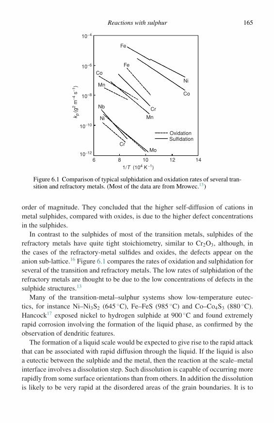
Reactions with sulphur 165
1/T (104 K−1)
k p (g
2 m
−4 s
−1)
10−4
10−6
10−8
10−10
10−12
6 8 10 12 14
Ni
Ni
Nb
Mn
Mn
Co
Co
Fe
Fe
Cr
Cr
OxidationSulfidation
Mo
Figure 6.1 Comparison of typical sulphidation and oxidation rates of several tran-sition and refractory metals. (Most of the data are from Mrowec.13)
order of magnitude. They concluded that the higher self-diffusion of cations inmetal sulphides, compared with oxides, is due to the higher defect concentrationsin the sulphides.
In contrast to the sulphides of most of the transition metals, sulphides of therefractory metals have quite tight stoichiometry, similar to Cr2O3, although, inthe cases of the refractory-metal sulfides and oxides, the defects appear on theanion sub-lattice.16 Figure 6.1 compares the rates of oxidation and sulphidation forseveral of the transition and refractory metals. The low rates of sulphidation of therefractory metals are thought to be due to the low concentrations of defects in thesulphide structures.13
Many of the transition-metal–sulphur systems show low-temperature eutec-tics, for instance Ni–Ni3S2 (645 ◦C), Fe–FeS (985 ◦C) and Co–Co4S3 (880 ◦C).Hancock17 exposed nickel to hydrogen sulphide at 900 ◦C and found extremelyrapid corrosion involving the formation of the liquid phase, as confirmed by theobservation of dendritic features.
The formation of a liquid scale would be expected to give rise to the rapid attackthat can be associated with rapid diffusion through the liquid. If the liquid is alsoa eutectic between the sulphide and the metal, then the reaction at the scale–metalinterface involves a dissolution step. Such dissolution is capable of occurring morerapidly from some surface orientations than from others. In addition the dissolutionis likely to be very rapid at the disordered areas of the grain boundaries. It is to
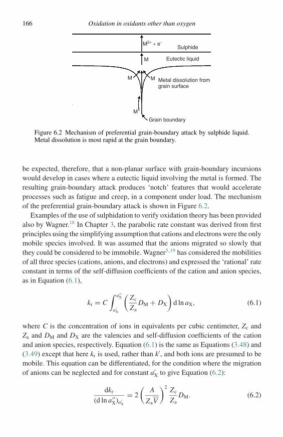
166 Oxidation in oxidants other than oxygen
M
MM
M
M2+ + e−
Eutectic liquid
Sulphide
Metal dissolution from grain surface
Grain boundary
Figure 6.2 Mechanism of preferential grain-boundary attack by sulphide liquid.Metal dissolution is most rapid at the grain boundary.
be expected, therefore, that a non-planar surface with grain-boundary incursionswould develop in cases where a eutectic liquid involving the metal is formed. Theresulting grain-boundary attack produces ‘notch’ features that would accelerateprocesses such as fatigue and creep, in a component under load. The mechanismof the preferential grain-boundary attack is shown in Figure 6.2.
Examples of the use of sulphidation to verify oxidation theory has been providedalso by Wagner.18 In Chapter 3, the parabolic rate constant was derived from firstprinciples using the simplifying assumption that cations and electrons were the onlymobile species involved. It was assumed that the anions migrated so slowly thatthey could be considered to be immobile. Wagner5,19 has considered the mobilitiesof all three species (cations, anions, and electrons) and expressed the ‘rational’ rateconstant in terms of the self-diffusion coefficients of the cation and anion species,as in Equation (6.1),
kr = C∫ a′′
X
a′X
(Zc
ZaDM + DX
)d ln aX, (6.1)
where C is the concentration of ions in equivalents per cubic centimeter, Zc andZa and DM and DX are the valencies and self-diffusion coefficients of the cationand anion species, respectively. Equation (6.1) is the same as Equations (3.48) and(3.49) except that here kr is used, rather than k′, and both ions are presumed to bemobile. This equation can be differentiated, for the condition where the migrationof anions can be neglected and for constant a′
X to give Equation (6.2):
dkr
(d ln a′′X)a′
X
= 2
(A
ZaV
)2 Zc
ZaDM. (6.2)
Reactions with sulphur 167
Mrowec16 measured the parabolic rate constant for the sulphidation of iron atdifferent sulphur activities in the atmosphere at 800 ◦C. By plotting the parabolic rateconstant against the logarithm of the sulphur activity the the tangent to the curve canbe used to obtain the cation diffusion coefficient as a function of the sulphur activity.The cation diffusion coefficient was found to be independent of the sulphur activitywith a value of 1.8 × 10⁻⁷ cm2 s−1. Radio active tracer experiments by Condit20
gave a value of 8.6 × 10⁻⁸ cm2 s−1 in good agreement, confirming Wagner’s modelfor high-temperature tarnishing reactions.
The usefulness and the hazards of marker experiments have also been demon-strated using sulphide systems. When using markers, a chemically inert materialis placed on the metal surface before exposure. After oxidation or sulphidation,the position of the marker with respect to the scale–metal interface should giveevidence regarding whether the scale grew predominantly by cation migration,anion migration, or both. If the scale is compact and free of pores, then a markerpositioned at the scale–metal interface infers that the scale has grown by outwarddiffusion of cations. Conversely, a marker found at the scale–gas interface, infersthat scale growth occurred by inward anion diffusion. It follows that, if cations andanions both are mobile to the same extent, the markers would be expected to befound in the middle of the scale. Unfortunately, markers found in the middle ofa scale pose a problem, since most compounds of which scales are formed usu-ally show predominant migration of one of the ionic species only. The locationof markers in the middle of scales is usually evidence that the scale has separ-ated from the metal substrate during growth or that species can be transported bymechanisms other than pure lattice diffusion. This has been discussed by severalworkers,19–23 whose publications should be consulted before undertaking markerexperiments.
The defect concentrations found in sulphides are so high that some interactionof defects is almost inevitable. In the case of iron sulphide, FeS, if there werelocalized electronic defects, the progressive ionization of defects could be expressedby Equations (6.3)–(6.5):
1
2S2(g) = SX
S + VFe, (6.3)
1
2S2(g) = SX
S + V′Fe + h., (6.4)
1
2S2(g) = SX
S + V′′Fe + 2h.. (6.5)
According to which expression prevails, the concentration of iron ion vacan-cies would be expressed in terms of the sulphur partial pressure as shown in
168 Oxidation in oxidants other than oxygen
Equations (6.6)–(6.8):
[VFe] = const.p1/2S2
, (6.6)
[V′
Fe
] = const.p1/4S2
, (6.7)
[V′′
Fe
] = const.p1/6S2
. (6.8)
Mrowec,16 using existing data24–26, calculated that the concentration of iron-ionvacancies was proportional to the sulphur partial pressure to the power of 1/1.9 at800 ◦C. This result is consistent with the metallic nature of FeS,1 i.e., there are aninsignificant number of localized electronic defects.
One final interesting point about sulphidation is that, because the free energiesof formation of the sulphides of iron, nickel, cobalt, chromium, and aluminium arequite similar, selective sulphidation of chromium and aluminium is not favouredas in the case of oxidation. Lai9 has reviewed the literature of the sulphidation ofalloys and has made several generalizations as follows.
(1) Alloys of iron, nickel, and cobalt sulphidize at similar rates – within an order of mag-nitude.
(2) Alloys containing less than 40% Cr may show improved sulphidation resistance byforming an inner layer of ternary sulphide or chromium sulphide. It has been foundthat Cr concentrations in excess of 17 wt% Cr provide some sulphidation protection insteels.27
(3) Alloys containing more than 40% Cr could form a single, protective, outer layer ofCr2S3. At the higher Cr levels, all three alloy systems showed similar resistance.
(4) The presence of Al in Fe and Co alloys could be beneficial due to the formation of analuminium-based sulphide. In the case of Ni-based alloys the results were erratic.
(5) However, formation of Al2S3 scales is not particularly useful because they react withH2O, even at room temperature.
On the other hand, refractory-metal sulphides are both very stable and slow growing.This has been addressed by Douglass and coworkers,28–35 who demonstrated thatthe addition of Mo and Mo plus Al to nickel substantially reduced the parabolic rateconstant for sulphidation, by about five orders of magnitude for the compositionNi–30 wt% Mo–8 wt% Al; and, in the case of iron alloys, by six orders of magnitudefor the composition Fe–30 wt% Mo– 5 wt% Al. In these cases the scales formedwere Al0.5Mo2S4, which gave excellent resistance to sulphidation, but would formmolybdenum oxides in oxidizing atmospheres.13
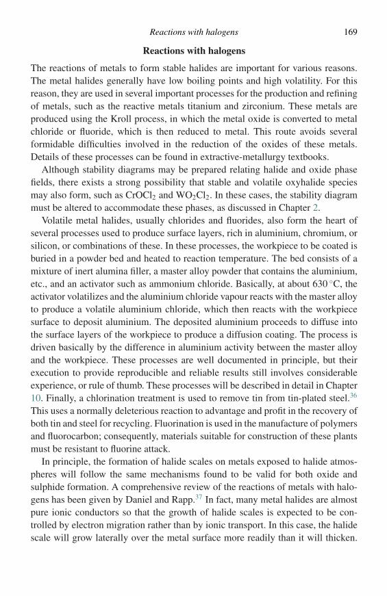
Reactions with halogens 169
Reactions with halogens
The reactions of metals to form stable halides are important for various reasons.The metal halides generally have low boiling points and high volatility. For thisreason, they are used in several important processes for the production and refiningof metals, such as the reactive metals titanium and zirconium. These metals areproduced using the Kroll process, in which the metal oxide is converted to metalchloride or fluoride, which is then reduced to metal. This route avoids severalformidable difficulties involved in the reduction of the oxides of these metals.Details of these processes can be found in extractive-metallurgy textbooks.
Although stability diagrams may be prepared relating halide and oxide phasefields, there exists a strong possibility that stable and volatile oxyhalide speciesmay also form, such as CrOCl2 and WO2Cl2. In these cases, the stability diagrammust be altered to accommodate these phases, as discussed in Chapter 2.
Volatile metal halides, usually chlorides and fluorides, also form the heart ofseveral processes used to produce surface layers, rich in aluminium, chromium, orsilicon, or combinations of these. In these processes, the workpiece to be coated isburied in a powder bed and heated to reaction temperature. The bed consists of amixture of inert alumina filler, a master alloy powder that contains the aluminium,etc., and an activator such as ammonium chloride. Basically, at about 630 ◦C, theactivator volatilizes and the aluminium chloride vapour reacts with the master alloyto produce a volatile aluminium chloride, which then reacts with the workpiecesurface to deposit aluminium. The deposited aluminium proceeds to diffuse intothe surface layers of the workpiece to produce a diffusion coating. The process isdriven basically by the difference in aluminium activity between the master alloyand the workpiece. These processes are well documented in principle, but theirexecution to provide reproducible and reliable results still involves considerableexperience, or rule of thumb. These processes will be described in detail in Chapter10. Finally, a chlorination treatment is used to remove tin from tin-plated steel.36
This uses a normally deleterious reaction to advantage and profit in the recovery ofboth tin and steel for recycling. Fluorination is used in the manufacture of polymersand fluorocarbon; consequently, materials suitable for construction of these plantsmust be resistant to fluorine attack.
In principle, the formation of halide scales on metals exposed to halide atmos-pheres will follow the same mechanisms found to be valid for both oxide andsulphide formation. A comprehensive review of the reactions of metals with halo-gens has been given by Daniel and Rapp.37 In fact, many metal halides are almostpure ionic conductors so that the growth of halide scales is expected to be con-trolled by electron migration rather than by ionic transport. In this case, the halidescale will grow laterally over the metal surface more readily than it will thicken.
170 Oxidation in oxidants other than oxygen
Agl
Ag
Ag+
e−
Pt
Figure 6.3 Growth of silver iodide on silver as it proceeds to cover a piece ofplatinum in electrical contact with the silver.
In fact a halide scale will grow beyond the reacting metal and over the surface ofan inert metal attached to it, by the mechanism proposed by Ilschner-Gench andWagner.38 In this mechanism, the ions migrate through the halide and the electronsmigrate through the inert metal to the reaction site. This mechanism is shown inFigure 6.3 for the case of the iodization of silver and indicates clearly how the lowelectronic conductivity of the halide emphasizes surface coverage rather than scalethickening. The ionic nature of PbI2 scales growing on Pb has been demonstratedby Kuiry et al.,39 who showed that scale growth rate was much more rapid whenthe electrons were shorted across the scale.
In common with oxide scales, halide scales can also suffer mechanical damagesuch as cracks, etc. In addition, the vapour pressure of the halide can be quite high,such that evaporation of the halide from the scale–gas interface can be substantial.This leads to simultaneous formation and evaporation of the halide scale and has alsobeen treated by Daniel and Rapp.37 The rate of thickening of a scale forming underthese conditions then follows paralinear kinetics40 as described for the combinedscale growth and evaporation of chromium oxide in Chapter 4.
Lai9 indicates that the addition of Cr and Ni to iron alloys improves their chlori-nation resistance. Consequently, nickel alloys are used for exposure to chlorine-bearing atmospheres. Most metals appear to resist attack up to a certain temperature,above which rapid attack ensues. This critical temperature for iron is about 250 ◦C,and 500 ◦C for nickel.9
Many environments contain oxygen and chlorine, in which case there is compe-tition to form a solid oxide layer or a volatile chloride. The tendency to form thevolatile chloride increases with chlorine partial pressure and temperature, as shownby Maloney and McNallen for cobalt.41 In general, alloys that contain molybdenumand tungsten do not perform well in halogen-bearing atmospheres because of theformation of their volatile oxychlorides MoO2Cl2 and WO2Cl2.42 In the presenceof oxygen and chlorine any reduction in reaction rate depends on whether or not aprotective oxide scale can form. According to Lai,9 this is possible in many engi-neering alloys above 900 ◦C, when aluminium is present and capable of formingan alumina scale.
Reactions with carbon 171
Fluorine attack follows the mechanisms mentioned for the case of chlorine.Namely, the reaction is slow at lower temperatures when a fluoride protective layeris formed; but at higher temperatures, the formation of liquid and, especially, volatilefluorides leads to rapid attack of the metal.
More detail of the response of alloys to atmospheres based on C12, H2–H2S,O2–C12, and corresponding fluorine atmospheres is given by Lai.9
The halogenation of metals provides opportunities to study scaling reactionsin which the reaction product is a pure ionic conductor, which can also behighly volatile. These systems can be studied at relatively low temperature; theyare important in their own right in terms of the mechanisms of extraction andchemical-vapour-deposition processes that employ gaseous halides as intermediatecompounds.
Reactions with carbon
In many processes, carbon is present as the primary or secondary oxidant. Wherecarbon is the primary oxidant, the principal reaction is that of carburization orthe dissolution of carbon into the metal matrix. The solubility of carbon in metalsvaries widely, being very low in Ni, Cu, Co, and ferritic iron but quite substantialin austenitic iron. Carburization of alloys, principally steels, is a common treat-ment for developing a hard and strong surface on components that are exposed tocontact wear during service. The theory and techniques for this are clarified in theliterature.43
Carbon may be introduced into the metal surface using several gas systemsinvolving reactions such as those shown in Equations (6.9)–(6.11):
CO (g) + H2(g) = C + H2O (g); �Go9, (6.9)
2CO (g) = C + CO2 (g); �Go10, (6.10)
CH4 (g) = C + 2H2 (g); �Go11. (6.11)
In each case, the carbon activity of the gas is given using the equilibrium constantof the reactions given in Equations (6.12)–(6.14):
aC = pCO pH2
pH2Oexp
(−�Go9
RT
), (6.12)
aC = p2CO
pCO2
exp
(−�Go10
RT
), (6.13)
aC = pCH4
p2H2
exp
(−�Go11
RT
). (6.14)
172 Oxidation in oxidants other than oxygen
Standard references9,43 contain diagrams that give the carbon activities of variousatmospheres over a range of temperatures. The time of treatment is controlled bythe diffusion of carbon into the component and depends upon the required surfaceconcentration, depth of carburized rim, temperature, and the diffusion coefficientof carbon. Treatments of this simple process, in cases of complete diffusion controlinvolve the solution of Fick’s second law44 for planar, cylindrical, or sphericalcoordinates, depending on the specimen dimensions and geometry.
Under most practical carburization conditions for steels the reaction rate is undermixed control of surface reaction and diffusion.45 Whereas the carburization ofsimple steels, for instance, is straightforward, and hardness is achieved by theformation of high-carbon martensite on heat treatment, the presence of carbonin stainless steels and superalloys results in the formation of carbides based onchromium and other alloying elements. Excessive carburization can result in theremoval from solution of protective elements such as chromium. This can seriouslyreduce the corrosion resistance of the component, particularly at grain boundaries.
Although carburization can enhance the performance of certain components, incases such as reformer tubes in the treatment of oil and hydrocarbons, carburizationof stainless steels is deleterious and life limiting. In this case internal carbides formwith kinetics analogous to those for internal oxidation.46 Consequently, alloys thatare resistant to carburization are developed, primarily by alloying with nickel toreduce the diffusion coefficient of carbon, and with silicon and aluminium, whichare thought to impart some protection by the formation of impervious silica andalumina surface films in the low-oxygen-potential atmospheres.10
Metal dusting is another carbon interaction that is harmful.47,48 In this reaction,the carbon activity in the gas must be greater than unity, and it appears that the carbonfrom the atmosphere gas species dissolves into the metal faster than it can nucleateas soot on the metal surface. This produces high carbon activities in the metal and,for the case of iron-base alloys, leads to the growth of metastable carbides, whichsubsequently decompose to a powdery product. These reactions occur typically inthe temperature range 450–800 ◦C.
Much of the work into the dusting attack of alloys has been carried out on nickel-and iron-based stainless systems similar to those used in reforming reactions wherethe phenomenon is a nuisance.47–49 The reaction is also dangerous in that it can leadto the perforation of tubes very rapidly, within a few hours, and it is found generallywhere metal components are in contact with carbonaceous gas mixtures of lowoxygen potential, typically CO–H2 mixtures, or atmospheres containing organicgases. Because the carbon activity of the atmosphere exceeds unity and because ofthe difficulty in nucleating graphite on the metal surface, without a catalyst, it ispossible for metastable carbides of the type M3C and M23C6 to form. Followingnucleation of graphite, these metastable carbides decompose to metal and carbon.Thus, the corrosion products of metal dusting attack are powdery mixtures of fine
Reactions with nitrogen 173
metal powder and carbon. The alloy is quite uniformly attacked in the case of lowalloy steels, but involves pitting in the cases of alloy steels and nickel-base alloys.The degradation of Ni-base alloys has been reported to occur by the formation ofgraphite without the intermediate formation of metastable carbides.50
Metal dusting of iron proceeds in five stages.51,52
(1) Carbon dissolves in the metal to a degree of supersaturation.(2) Cementite precipitates at the metal surface and in grain boundaries.(3) Graphite deposits from the atmosphere on to the cementite.(4) The cementite begins to decompose forming graphite and metal particles.(5) Further graphite deposition proceeds, catalyzed by the metal particles.
Similar mechanisms are thought to be valid for low alloy steels.In the case of high alloy steels that contain high concentrations of chromium, a
protective scale of chromium oxides is formed. Where this scale fails locally, thedusting sequence can proceed since carbon can only penetrate the scale at defects.This results in the formation of a pitted surface, beginning with small pits, whichwiden to larger hemispherical sites with time. It is feasible that, if the chromiascale could be made more secure, the steel would show improved resistance tometal dusting. It has been observed that surface working is effective in improvingthe protectiveness of the chromia scales.53,54 It should be recognized, however,that this increased resistance is not stable and that failure would be swift, once thesequence of dusting is begun.
In practice, it is found that the presence of sulphur in the atmosphere in the formof H2S effectively suppresses metal dusting. This is thought54–57 to result from thesuppression of graphite nucleation by the sulphur, which thereby halts the chain ofdusting reactions.
Reactions with nitrogen
There have been a number of studies directed towards the effects of nitrogen onhigh-temperature corrosion of metals.9,58–63 Pettit et al.58 oxidized pure chromiumin air at 1200 ◦C and found an external scale of chromia to be formed together witha layer of chromium nitride, Cr2N, that formed immediately on top of the metal.This structure is consistent if the nitrogen is transported through the chromia layerto form nitride at the metal surface. Perkins59 observed very similar results for aseries of chromium alloys oxidized in air at 1150 ◦C. Most of the alloys also showedinternal nitridation. It was found that alloy surface preparation could influence therate of transport of nitrogen through the chromia scales.
When iron-, nickel-, and cobalt-base alloys containing chromium were oxidizedin air at 900 ◦C for 25 h60 only oxide scales were formed and nitride formationwas observed only on a Co–35 wt% Cr alloy. Presumably the inward diffusion of
174 Oxidation in oxidants other than oxygen
nitrogen through the chromia scale occurred in all cases but only the Co–35 wt% Cralloy has a high enough Cr activity to form the nitride. The presence of nitrogen didnot alter the isothermal behaviour of the alloys, but extensive internal precipitationoccurred on cyclic oxidation of Ni–25 wt% Cr–6 wt% Al and Co–25 wt% Cr–6wt% Al alloys. It appears that the inclusion of nitrogen into the metal substrate,with resultant nitride precipitation and, perhaps, embrittlement, may be the maincauses of a detrimental effect of nitrogen.
References
1. H. Rau, J. Phys. Chem. Solids, 37 (1976), 425.2. H. Rickert, Z. Phy. Chem. NF, 23 (1960), 355.3. S. Mrowec and H. Rickert, Z. Phy. Chem. NF, 28 (1961), 422.4. S. Mrowec and H. Rickert, Z. Phy. Chem. NF, 36 (1963), 22.5. C. Z. Wagner, Phys. Chem. B, 21 (1933), 25.6. S. Mrowec and T. Werber, Gas Corrosion of Metals, Springfield, VA, National
Technical Information Service, 1978, p. 383.7. S. Mrowec and K. Przybylski, High Temp. Mater., 6 (1984), 1.8. D. J. Young, Rev. High Temp. Mater., 4 (1980), 229.9. G. Y. Lai, High Temperature Corrosion of Engineering Alloys, Materials Park, OH,
ASM International, 1990.10. S. Wegge and H. J. Grabke, Werkst. u. Korr., 43 (1992), 437.11. W. L. Worrell and H. Kaplan, in Heterogenous Kinetics at Elevated Temperatures,
eds. W. L. Worrell and G. R. Belton, New York, Plenum Press, 1970, p. 113.12. K. N. Strafford, The sulfidation of metals and alloys, Metallurgical Review No. 138,
Met. Mater., 3 (1969), 409.13. S. Mrowec, Oxid. Met., 44 (1995), 177.14. Y. Fueki, Y. Oguri, and T. Mukaibo, Bull. Chem. Soc. Jpn., 41 (1968), 569.15. S. Mrowec and K. Przybylski, High Temp. Mater. Process, 6 (1984), 1.16. S. Mrowec, Bull. Acad. Polon. Sci., 15 (1967), 517.17. P. Hancock, First International Conference on Metallic Corrosion, London,
Butterworth, 1962, p. 193.18. C. Wagner, Pittsburgh International Conference on Surface Reactions, Pittsburgh,
PA, Corrosion Publishing Company, 1948, p. 77.19. C. Wagner, Atom Movements, Cleveland, OH, ASM, 1951, p. 153.20. R. Condit, Kinetics of High Temperature Processes, ed. W. D. Kingery, New York,
John Wiley, 1959, p. 97.21. A. Bruckman, Corr. Sci., 7 (1967), 51.22. M. Cagnet and J. Moreau, Acta. Met., 7 (1959), 427.23. R. A. Meussner and C. E. Birchenall, Corrosion, 13 (1957), 677.24. S. Mrowec, Z. Phys. Chem. NF, 29 (1961), 47.25. P. Kofstad, P. B. Anderson, and O. J. Krudtaa, J. Less Comm. Met., 3 (1961), 89.26. T. Rosenqvist, J. Iron Steel Inst., 179 (1954), 37.27. W. Grosser, D. Meder, W. Auer, and H. Kaesche, Werkst. u. Korr., 43 (1992), 145.28. M. F. Chen and D. L. Douglass, Oxid. Met., 32 (1989), 185.29. R. V. Carter, D. L. Douglass, and F. Gesmundo, Oxid. Met., 31 (1989),
341.30. B. Gleeson, D. L. Douglass, and F. Gesmundo, Oxid. Met., 31 (1989), 209.
References 175
31. M. F. Chen, D. L. Douglass, and F. Gesmundo, Oxid. Met., 31 (1989), 237.32. G. Wang, R. V. Carter, and D. L. Douglass, Oxid. Met., 32 (1989), 273.33. B. Gleeson, D. L. Douglass, and F. Gesmundo, Oxid. Met., 33 (1990), 425.34. G. Wang, D. L. Douglass, and F. Gesmundo, Oxid. Met., 35 (1991), 279.35. G. Wang, D. L. Douglass, and F. Gesmundo, Oxid Met., 35 (1991), 349.36. C. L. Marshall, Tin, New York, Reinhold, 1949.37. P. L. Daniel and R. A. Rapp, Advances in Corrosion Science and Technology, eds. M.
G. Fontana and R. W. Staehle, New York, Plenum Press, 1980.38. C. Ilschner-Gensch and C. Wagner, J. Electrochem. Soc., 105 (1958), 198.39. S. C. Kuiry, S. K. Roy, and S. K. Bose, Oxid. Met., 46 (1996), 399.40. C. S. Tedmon, J. Electrochem Soc., 113 (1966), 766.41. M. J. Maloney and M. J. McNallen, Met. Trans. B, 16 (1983), 751.42. J. M. Oh, M. J. McNallen, G. Y. Lai, and M. F. Rothman, Met. Trans. A, 17 (1986),
1087.43. Metals Handbook, 10th edn, Metals Park, OH, ASM International, 1991, vol. 4, p.
542.44. J. Crank, Mathematics of Diffusion, Oxford, UK, Oxford University Press, 1956.45. H-. J. Grabke, Hart.-Tech. Mitt., 45 (1990), 110.46. A. Schnaas and H.-J. Grabke, Oxid. Met., 12 (1979), 387.47. R. F. Hochmann, Catastrophic deterioration of high-temperature alloys in
carbonaceous atmospheres. In Properties of High-Temperature Alloys, eds. A.Foroulis and F. S. Pettit, Princeton, NJ, Electrochemical Society, 1977, p. 715.
48. H. J. Grabke, Corrosion, 51 (1995), 711.49. G. H. Meier, R. A. Perkins, and W. C. Coons, Oxid. Met., 17 (1982), 235.50. H. J. Grabke, Corrosion, 56 (2000), 801.51. H. J. Grabke, R. Krajak, and J. C. Nava Paz, Corrosion Sci., 35 (1998), 1141.52. H. J. Grabke, Mater. Corr., 49 (1998), 303.53. H. J. Grabke, E. M. Muller-Lorenz, B. Eltester, M. Lucas, and D. Monceau, Steel
Res., 68 (1997), 179.54. H. J. Grabke, E. M. Muller-Lorenz, and S. Strauss, Oxid. Met., 50 (1998), 241.55. Y. Inokuti, Trans. Iron Steel Inst. Jpn., 15 (1975), 314, 324.56. H. J. Grabke and E. M. Muller-Lorenz, Steel Res., 66 (1995), 252.57. A. Schneider, H. Viefhaus, G. Inden, H. J. Grabke, and E. M. Muller-Lorenz, Mater.
Corr., 49 (1998), 330.58. F. S. Pettit, J. A. Goebel, and G. W. Goward, Corr. Sci., 9 (1969), 903.59. R. A. Perkins, Alloying of chromium to resist nitridation, NASA Report
NASA-Cr-72892, July, 1971.60. C. S. Giggins and F. S. Pettit, Oxid. Met., 14 (1980), 363.61. I. Aydin, H. E. Buhler, and A. Rahmel, Werkst. u. Korr., 31 (1980), 675.62. U. Jakel and W. Schwenk, Werkst. u. Korr., 22 (1971), 1.63. H-. J. Grabke, S. Strauss, and D. Vogel, Mater. Corr., 54 (2003), 895.
7
Reactions of metals in mixed environments
Introduction
Study of the behaviour of pure metals and alloys in single oxidant systems, at hightemperature, is vital for developing an understanding of the general mechanismsinvolved in oxidation and scaling reactions. In almost all cases where alloys areused commercially at high temperature, in gas turbines, in heat exchangers, orstructurally in furnaces etc., they are exposed to complex atmospheres that containa variety of gas species. These situations are complex and demand a thoroughunderstanding of the underlying thermodynamics and kinetic principles to describethe reactions and the mechanisms by which they proceed. In such cases the aim isnot simply to explain and understand how the reaction proceeds, but to go a stepfurther and predict how the reactions might be prevented or contained.
In fact, apart from controlled laboratory atmospheres, the gas is always complexin the multi-oxidant sense since even nitrogen in air can form nitrides with somealloy systems in addition to the oxides formed by the oxygen. This is seen particu-larly in alloys containing metals such as chromium, titanium, and niobium, wherethe formation of nitrides in air atmospheres interferes with the ‘simple’ oxidationsituation that is observed when using pure oxygen, or oxygen–argon mixtures.1,2
Air–H2O and air–CO2 atmospheres
The presence of water vapour and carbon dioxide in air and, to a greater extent, inatmospheres derived from the combustion of fossil fuel, has been found to increasethe observed reaction rate of steels and other metals noticeably. This was studiedand explained by Rahmel and Tobolski3 who proposed that the gases set up redoxsystems of H2–H2O and CO–CO2 to transfer oxygen across pores in the oxidestructure. When a pore develops in a scale, forming on a metal exposed to air, it isassumed that the total pressure within the pore is the same as that of the external
176
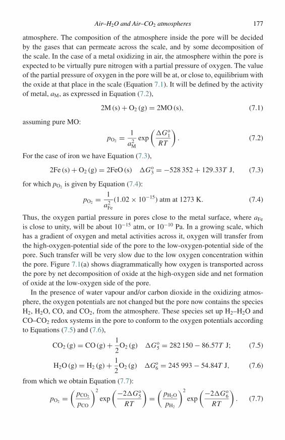
Air–H2O and Air–CO2 atmospheres 177
atmosphere. The composition of the atmosphere inside the pore will be decidedby the gases that can permeate across the scale, and by some decomposition ofthe scale. In the case of a metal oxidizing in air, the atmosphere within the pore isexpected to be virtually pure nitrogen with a partial pressure of oxygen. The valueof the partial pressure of oxygen in the pore will be at, or close to, equilibrium withthe oxide at that place in the scale (Equation 7.1). It will be defined by the activityof metal, aM, as expressed in Equation (7.2),
2M (s) + O2 (g) = 2MO (s), (7.1)
assuming pure MO:
pO2 = 1
a2M
exp
(�Go
1
RT
). (7.2)
For the case of iron we have Equation (7.3),
2Fe (s) + O2 (g) = 2FeO (s) �Go3 = −528 352 + 129.33T J, (7.3)
for which pO2 is given by Equation (7.4):
pO2 = 1
a2Fe
(1.02 × 10⁻¹⁵) atm at 1273 K. (7.4)
Thus, the oxygen partial pressure in pores close to the metal surface, where aFe
is close to unity, will be about 10−15 atm, or 10−10 Pa. In a growing scale, whichhas a gradient of oxygen and metal activities across it, oxygen will transfer fromthe high-oxygen-potential side of the pore to the low-oxygen-potential side of thepore. Such transfer will be very slow due to the low oxygen concentration withinthe pore. Figure 7.1(a) shows diagrammatically how oxygen is transported acrossthe pore by net decomposition of oxide at the high-oxygen side and net formationof oxide at the low-oxygen side of the pore.
In the presence of water vapour and/or carbon dioxide in the oxidizing atmos-phere, the oxygen potentials are not changed but the pore now contains the speciesH2, H2O, CO, and CO2, from the atmosphere. These species set up H2–H2O andCO–CO2 redox systems in the pore to conform to the oxygen potentials accordingto Equations (7.5) and (7.6),
CO2 (g) = CO (g) + 1
2O2 (g) �Go
5 = 282 150 − 86.57T J; (7.5)
H2O (g) = H2 (g) + 1
2O2 (g) �Go
6 = 245 993 − 54.84T J, (7.6)
from which we obtain Equation (7.7):
pO2 =(
pCO2
pCO
)2
exp
(−2�Go5
RT
)=
(pH2O
pH2
)2
exp
(−2�Go6
RT
). (7.7)
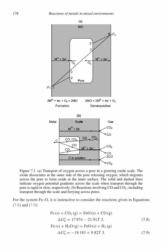
178 Reactions of metals in mixed environments
(a)
p 2O′
p 2O′′
(b)
Figure 7.1 (a) Transport of oxygen across a pore in a growing oxide scale. Theoxide dissociates at the outer side of the pore releasing oxygen, which migratesacross the pore to form oxide at the inner surface. The solid and dashed linesindicate oxygen potential gradients across the scale when transport through thepore is rapid or slow, respectively. (b) Reactions involving CO and CO2, includingtransport through the scale and ferrying across pores.
For the system Fe–O, it is instructive to consider the reactions given in Equations(7.8) and (7.9):
Fe (s) + CO2 (g) = FeO (s) + CO (g)
�Go8 = 17 974 − 21.91T J, (7.8)
Fe (s) + H2O (g) = FeO (s) + H2 (g)
�Go9 = −18 183 + 9.82T J. (7.9)
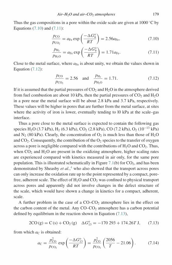
Air–H2O and air–CO2 atmospheres 179
Thus the gas compositions in a pore within the oxide scale are given at 1000 ◦C byEquations (7.10) and (7.11):
pCO
pCO2
= aFe exp
(−�Go8
RT
)= 2.56aFe, (7.10)
pH2
pH2O= aFe exp
(−�Go9
RT
)= 1.71aFe. (7.11)
Close to the metal surface, where aFe is about unity, we obtain the values shown inEquation (7.12):
pCO
pCO2
= 2.56 andpH2
pH2O= 1.71. (7.12)
If it is assumed that the partial pressures of CO2 and H2O in the atmosphere derivedfrom fuel combustion are about 10 kPa, then the partial pressures of CO2 and H2Oin a pore near the metal surface will be about 2.8 kPa and 3.7 kPa, respectively.These values will be higher in pores that are further from the metal surface, at siteswhere the activity of iron is lower, eventually tending to l0 kPa at the scale–gasinterface.
Thus a pore close to the metal surface is expected to contain the following gasspecies H2O (3.7 kPa), H2 (6.3 kPa), CO2 (2.8 kPa), CO (7.2 kPa), O2 (10−13 kPa)and N2 (80 kPa). Clearly, the concentration of O2 is much less than those of H2Oand CO2. Consequently, the contribution of the O2 species to the transfer of oxygenacross a pore is negligible compared with the contributions of H2O and CO2. Thus,when CO2 and H2O are present in the oxidizing atmosphere, higher scaling ratesare experienced compared with kinetics measured in air only, for the same porepopulation. This is illustrated schematically in Figure 7.1(b) for CO2, and has beendemonstrated by Sheasby et al.,4 who also showed that the transport across porescan only increase the oxidation rate up to the point represented by a compact, pore-free, adherent scale. The effect of H2O and CO2 was confined to physical transportacross pores and apparently did not involve changes in the defect structure ofthe scale, which would have shown a change in kinetics for a compact, adherent,scale.
A further problem in the case of a CO–CO2 atmosphere lies in the effect onthe carbon content of the metal. Any CO–CO2 atmosphere has a carbon potentialdefined by equilibrium in the reaction shown in Equation (7.13),
2CO (g) = C (s) + CO2 (g) �Go13 = −170 293 + 174.26T J, (7.13)
from which aC is obtained:
aC = p2CO
pCO2
exp
(−�Go13
RT
)= p2
CO
pCO2
(2056
T− 21.06
). (7.14)
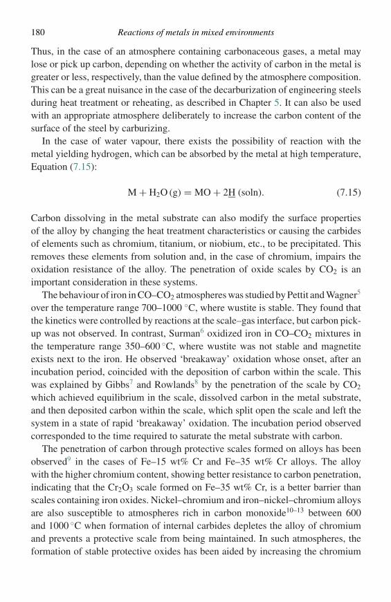
180 Reactions of metals in mixed environments
Thus, in the case of an atmosphere containing carbonaceous gases, a metal maylose or pick up carbon, depending on whether the activity of carbon in the metal isgreater or less, respectively, than the value defined by the atmosphere composition.This can be a great nuisance in the case of the decarburization of engineering steelsduring heat treatment or reheating, as described in Chapter 5. It can also be usedwith an appropriate atmosphere deliberately to increase the carbon content of thesurface of the steel by carburizing.
In the case of water vapour, there exists the possibility of reaction with themetal yielding hydrogen, which can be absorbed by the metal at high temperature,Equation (7.15):
M + H2O (g) = MO + 2H (soln). (7.15)
Carbon dissolving in the metal substrate can also modify the surface propertiesof the alloy by changing the heat treatment characteristics or causing the carbidesof elements such as chromium, titanium, or niobium, etc., to be precipitated. Thisremoves these elements from solution and, in the case of chromium, impairs theoxidation resistance of the alloy. The penetration of oxide scales by CO2 is animportant consideration in these systems.
The behaviour of iron in CO–CO2 atmospheres was studied by Pettit and Wagner5
over the temperature range 700–1000 ◦C, where wustite is stable. They found thatthe kinetics were controlled by reactions at the scale–gas interface, but carbon pick-up was not observed. In contrast, Surman6 oxidized iron in CO–CO2 mixtures inthe temperature range 350–600 ◦C, where wustite was not stable and magnetiteexists next to the iron. He observed ‘breakaway’ oxidation whose onset, after anincubation period, coincided with the deposition of carbon within the scale. Thiswas explained by Gibbs7 and Rowlands8 by the penetration of the scale by CO2
which achieved equilibrium in the scale, dissolved carbon in the metal substrate,and then deposited carbon within the scale, which split open the scale and left thesystem in a state of rapid ‘breakaway’ oxidation. The incubation period observedcorresponded to the time required to saturate the metal substrate with carbon.
The penetration of carbon through protective scales formed on alloys has beenobserved9 in the cases of Fe–15 wt% Cr and Fe–35 wt% Cr alloys. The alloywith the higher chromium content, showing better resistance to carbon penetration,indicating that the Cr2O3 scale formed on Fe–35 wt% Cr, is a better barrier thanscales containing iron oxides. Nickel–chromium and iron–nickel–chromium alloysare also susceptible to atmospheres rich in carbon monoxide10–13 between 600and 1000 ◦C when formation of internal carbides depletes the alloy of chromiumand prevents a protective scale from being maintained. In such atmospheres, theformation of stable protective oxides has been aided by increasing the chromium
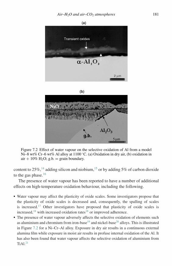
Air–H2O and air–CO2 atmospheres 181
(a)
(b)
Figure 7.2 Effect of water vapour on the selective oxidation of Al from a modelNi–8 wt% Cr–6 wt% Al alloy at 1100 ◦C. (a) Oxidation in dry air, (b) oxidation inair + 10% H2O; g.b. = grain boundary.
content to 25%,14 adding silicon and niobium,15 or by adding 5% of carbon dioxideto the gas phase.16
The presence of water vapour has been reported to have a number of additionaleffects on high-temperature oxidation behaviour, including the following.
� Water vapour may affect the plasticity of oxide scales. Some investigators propose thatthe plasticity of oxide scales is decreased and, consequently, the spalling of scalesis increased.17 Other investigators have proposed that plasticity of oxide scales isincreased,18 with increased oxidation rates18 or improved adherence.
� The presence of water vapour adversely affects the selective oxidation of elements suchas aluminium and chromium from iron-base19 and nickel-base20 alloys. This is illustratedin Figure 7.2 for a Ni–Cr–Al alloy. Exposure in dry air results in a continuous externalalumina film while exposure in moist air results in profuse internal oxidation of the Al. Ithas also been found that water vapour affects the selective oxidation of aluminium fromTiAl.21
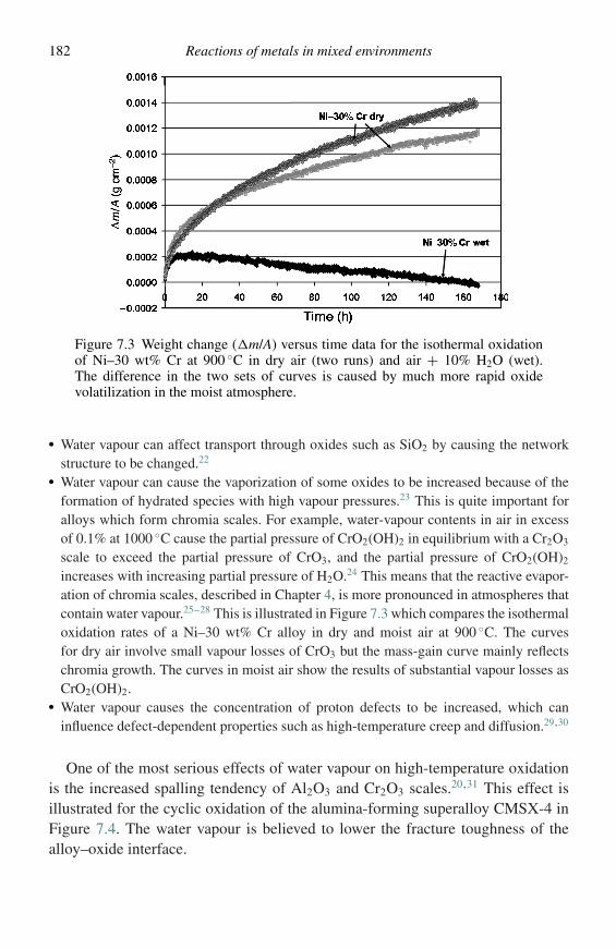
182 Reactions of metals in mixed environments
Figure 7.3 Weight change (�m/A) versus time data for the isothermal oxidationof Ni–30 wt% Cr at 900 ◦C in dry air (two runs) and air + 10% H2O (wet).The difference in the two sets of curves is caused by much more rapid oxidevolatilization in the moist atmosphere.
� Water vapour can affect transport through oxides such as SiO2 by causing the networkstructure to be changed.22
� Water vapour can cause the vaporization of some oxides to be increased because of theformation of hydrated species with high vapour pressures.23 This is quite important foralloys which form chromia scales. For example, water-vapour contents in air in excessof 0.1% at 1000 ◦C cause the partial pressure of CrO2(OH)2 in equilibrium with a Cr2O3
scale to exceed the partial pressure of CrO3, and the partial pressure of CrO2(OH)2
increases with increasing partial pressure of H2O.24 This means that the reactive evapor-ation of chromia scales, described in Chapter 4, is more pronounced in atmospheres thatcontain water vapour.25–28 This is illustrated in Figure 7.3 which compares the isothermaloxidation rates of a Ni–30 wt% Cr alloy in dry and moist air at 900 ◦C. The curvesfor dry air involve small vapour losses of CrO3 but the mass-gain curve mainly reflectschromia growth. The curves in moist air show the results of substantial vapour losses asCrO2(OH)2.
� Water vapour causes the concentration of proton defects to be increased, which caninfluence defect-dependent properties such as high-temperature creep and diffusion.29,30
One of the most serious effects of water vapour on high-temperature oxidationis the increased spalling tendency of Al2O3 and Cr2O3 scales.20,31 This effect isillustrated for the cyclic oxidation of the alumina-forming superalloy CMSX-4 inFigure 7.4. The water vapour is believed to lower the fracture toughness of thealloy–oxide interface.
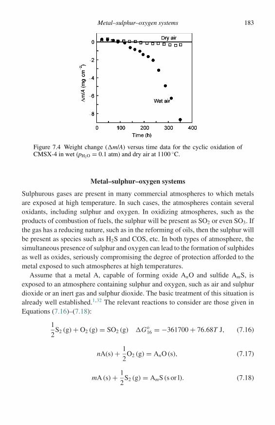
Metal–sulphur–oxygen systems 183
Figure 7.4 Weight change (�m/A) versus time data for the cyclic oxidation ofCMSX-4 in wet (pH2O = 0.1 atm) and dry air at 1100 ◦C.
Metal–sulphur–oxygen systems
Sulphurous gases are present in many commercial atmospheres to which metalsare exposed at high temperature. In such cases, the atmospheres contain severaloxidants, including sulphur and oxygen. In oxidizing atmospheres, such as theproducts of combustion of fuels, the sulphur will be present as SO2 or even SO3. Ifthe gas has a reducing nature, such as in the reforming of oils, then the sulphur willbe present as species such as H2S and COS, etc. In both types of atmosphere, thesimultaneous presence of sulphur and oxygen can lead to the formation of sulphidesas well as oxides, seriously compromising the degree of protection afforded to themetal exposed to such atmospheres at high temperatures.
Assume that a metal A, capable of forming oxide AnO and sulfide AmS, isexposed to an atmosphere containing sulphur and oxygen, such as air and sulphurdioxide or an inert gas and sulphur dioxide. The basic treatment of this situation isalready well established.1,32 The relevant reactions to consider are those given inEquations (7.16)–(7.18):
1
2S2 (g) + O2 (g) = SO2 (g) �Go
16 = −361700 + 76.68T J, (7.16)
nA(s) + 1
2O2 (g) = AnO (s), (7.17)
mA (s) + 1
2S2 (g) = AmS (s or l). (7.18)
184 Reactions of metals in mixed environments
According to the equilibrium in Equation (7.16), the sulphur potential of the atmo-sphere is given by Equation (7.19):
pS2 =(
pSO2
pO2
)2
exp
(2�Go
16
RT
). (7.19)
By considering the equilibria for the reactions shown in Equations (7.17) and (7.18),it can be seen that formation of oxide and sulphide can proceed if the partialpressures of O2 and S2 are sufficiently high, Equations (7.20) and (7.21):
pO2 >a2
AnO
a2nA
exp
(2�Go
17
RT
), (7.20)
pS2 >a2
AmS
a2mA
exp
(2�Go
18
RT
). (7.21)
In these equations aA is the activity of A, and aAnO and aAmS are the activities ofthe oxide and sulphide, respectively. If it is assumed that the oxide and sulphideare immiscible, then the oxide and sulphide activities can be taken to be unity forthe A–S–O system. Similarly, at the metal–scale interface the metal activity will beunity but it will fall throughout the scale towards the scale–gas interface.
The value of the metal activity at the scale–gas interface, a′′M, depends on which
reaction step is rate determining. The value of a′′M will be highest if the rate-
determining step is a surface reaction or transport through the gas phase to thescale surface. If the reaction rate is determined by diffusion through the scale thenthe value of a′′
M will be lower and in, or close to, equilibrium with the atmos-phere. This was indicated clearly by Rahmel and Gonzales33 and is shown inFigure 7.5.
From the phase stability diagram of a metal–sulphur–oxygen system, as shownin Figure 7.6, it should be possible to predict which phase will be present in thescale, given the atmosphere composition.
If the atmosphere composition were to lie within a single-phase field and thereaction were to proceed to completion, only a single phase would be produced,either oxide, sulphide, or sulphate. During reaction, however, only the scale–gasinterface is in equilibrium with the gas phase. Even so, for atmospheres withinsingle-phase fields, single-phase scales might be expected. The only exceptionwould be for atmospheres lying along boundaries such as the AnO/AmS boundaryin Figure 7.7, which corresponds to equilibrium in the displacement reaction shownin Equation (7.22):
nAmS + m
2O2 = mAnO + n
2S2. (7.22)
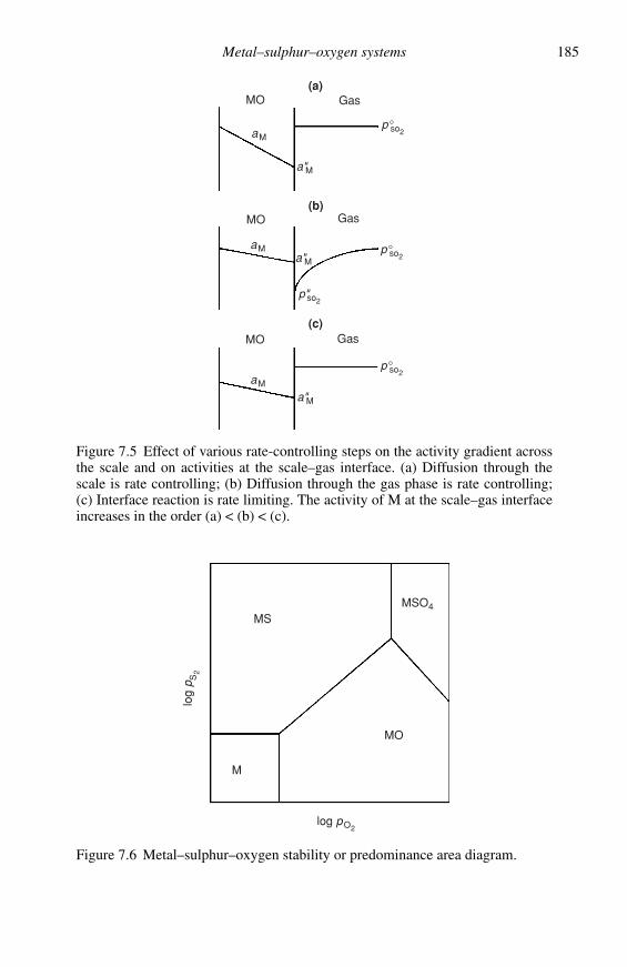
Metal–sulphur–oxygen systems 185
(a)
(b)
(c)
p°so2
p°so2
p°so2
p"so2
MO
MO
MO
Gas
Gas
Gas
aM
a"M
a"M
a"M
aM
aM
Figure 7.5 Effect of various rate-controlling steps on the activity gradient acrossthe scale and on activities at the scale–gas interface. (a) Diffusion through thescale is rate controlling; (b) Diffusion through the gas phase is rate controlling;(c) Interface reaction is rate limiting. The activity of M at the scale–gas interfaceincreases in the order (a) < (b) < (c).
MS
MO
M
MSO4
log pO2
log
p S2
Figure 7.6 Metal–sulphur–oxygen stability or predominance area diagram.
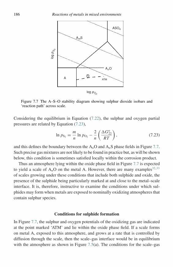
186 Reactions of metals in mixed environments
ATM
AnO
ASO4
AmS
log pO2
log
pS
2
A
Figure 7.7 The A–S–O stability diagram showing sulphur dioxide isobars and‘reaction path’ across scale.
Considering the equilibrium in Equation (7.22), the sulphur and oxygen partialpressures are related by Equation (7.23),
ln pS2 = m
nln pO2 − 2
n
(�Go
22
RT
), (7.23)
and this defines the boundary between the AnO and AnS phase fields in Figure 7.7.Such precise gas mixtures are not likely to be found in practice but, as will be shownbelow, this condition is sometimes satisfied locally within the corrosion product.
Thus an atmosphere lying within the oxide phase field in Figure 7.7 is expectedto yield a scale of AnO on the metal A. However, there are many examples32,33
of scales growing under these conditions that include both sulphide and oxide, thepresence of the sulphide being particularly marked at and close to the metal–scaleinterface. It is, therefore, instructive to examine the conditions under which sul-phides may form when metals are exposed to nominally oxidizing atmospheres thatcontain sulphur species.
Conditions for sulphide formation
In Figure 7.7, the sulphur and oxygen potentials of the oxidizing gas are indicatedat the point marked ‘ATM’ and lie within the oxide phase field. If a scale formson metal A, exposed to this atmosphere, and grows at a rate that is controlled bydiffusion through the scale, then the scale–gas interface would be in equilibriumwith the atmosphere as shown in Figure 7.5(a). The conditions for the scale–gas
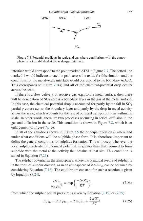
Conditions for sulphide formation 187
p"
p°
Figure 7.8 Potential gradients in scale and gas where equilibrium with the atmos-phere is not established at the scale–gas interface.
interface would correspond to the point marked ATM in Figure 7.7. The dotted linemarked 1 would indicate a reaction path across the oxide for this situation and theconditions for the metal–scale interface would correspond to the boundary A/AnO.This corresponds to Figure 7.5(a) and all of the chemical-potential drop occursacross the scale.
If there is a slow delivery of reactive gas, e.g., to the metal surface, then therewill be denudation of SO2 across a boundary layer in the gas at the metal surface.In this case, the chemical-potential drop is accounted for partly by the fall in SO2
partial pressure across the boundary layer and partly by the drop in metal activityacross the scale, which accounts for the rate of outward transport of ions within thescale. In other words, there are two processes occurring in series, diffusion in thegas and diffusion in the scale. This condition is shown in Figure 7.8, which is anenlargement of Figure 7.5(b).
In all of the situations shown in Figure 7.5 the principal question is where andunder what conditions will the sulphide phase form. It is, therefore, important todefine the general conditions for sulphide formation. This will occur whenever thelocal sulphur activity, or chemical potential, is greater than that required to formsulphide with the metal at the activity that obtains at that site. This condition isstated in Equation (7.21).
The sulphur potential in the atmosphere, where the principal source of sulphur isin the form of sulphur dioxide, as in an atmosphere of Ar–SO2, can be obtained byconsidering Equation (7.16). The equilibrium constant for such a reaction is givenby Equation (7.24),
pSO2
pO2 p1/2S2
= exp
(−�Go16
RT
), (7.24)
from which the sulphur partial pressure is given by Equation (7.19) or (7.25):
ln pS2 = 2 ln pSO2 − 2 ln pO2 + 2�Go16
RT. (7.25)
188 Reactions of metals in mixed environments
Assuming that there is no intersolubility between the sulphide and oxide phases,the oxide and sulphide would be formed at unit activity and the conditions for theirformation would be, from Equations (7.20) and (7.21), expressed, respectively, byEquations (7.26) and (7.27):
pO2 >1
a2nA
exp
(2�Go
17
RT
), (7.26)
pS2 >1
a2mA
exp
(2�Go
18
RT
). (7.27)
Consequently, the condition for sulphide formation at any place is given bycombining Equations (7.19) and (7.27) as in Equation (7.28):(
pSO2
pO2
)2
exp
(2�Go
16
RT
)>
1
a2mA
exp
(2�Go
18
RT
). (7.28)
The oxygen potential at any place within the scale is controlled by the metal activityat that site, as expressed by the identity in Equation (7.26), which may be substitutedin Equation (7.28):
pSO2
1
a2nA
exp
(2�Go
17
RT
)
2
exp
(2�Go
16
RT
)>
1
a2mA
exp
(2�Go
18
RT
). (7.29)
Rearranging Equation (7.29) indicates that the critical value of sulphur partial pres-sure at any site is determined by the metal activity at that site as shown in Equation(7.30),
pSO2 >1
a2nA
exp
(2�Go
17
RT
)exp
(−�Go16
RT
)· 1
amA
exp
(�Go
18
RT
), (7.30)
or Equation (7.31),
pSO2 >1
a(2n+m)A
exp
[1
RT
(2�Go
17 − �Go16 + �Go
18
)]. (7.31)
In using Equation (7.31) it is important to emphasize that its derivation has beenobtained assuming the activities of AmS and AnO are unity and that the two phasesare in equilibrium. Hence, Equation (7.31) is only applicable to the AmS/AnOboundary in Figure 7.7. From Equation (7.31) it is seen that the site at which sulphideis most likely to form, for a given value of pSO2 , is at the metal–scale interfacewhere the metal activity is a maximum at unity. This situation is described by
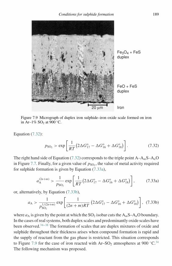
Conditions for sulphide formation 189
Fe3O4 + FeSduplex
FeO + FeSduplex
Iron20 µm
Figure 7.9 Micrograph of duplex iron sulphide–iron oxide scale formed on ironin Ar–1% SO2 at 900 ◦C.
Equation (7.32):
pSO2 > exp
[1
RT
(2�Go
17 − �Go16 + �Go
18
)]. (7.32)
The right hand side of Equation (7.32) corresponds to the triple point A–AmS–AnOin Figure 7.7. Finally, for a given value of pSO2 , the value of metal activity requiredfor sulphide formation is given by Equation (7.33a),
a(2n+m)A >
1
pSO2
exp
[1
RT
(2�Go
17 − �Go16 + �Go
18
)], (7.33a)
or, alternatively, by Equation (7.33b),
aA >1
p1/(2n+m)SO2
exp
[1
(2n + m)RT
(2�Go
17 − �Go16 + �Go
18
)], (7.33b)
where aA is given by the point at which the SO2 isobar cuts the AmS–AnO boundary.In the cases of real systems, both duplex scales and predominantly oxide scales havebeen observed.34–38 The formation of scales that are duplex mixtures of oxide andsulphide throughout their thickness arises when compound formation is rapid andthe supply of reactant from the gas phase is restricted. This situation correspondsto Figure 7.9 for the case of iron reacted with Ar–SO2 atmospheres at 900 ◦C.34
The following mechanism was proposed.
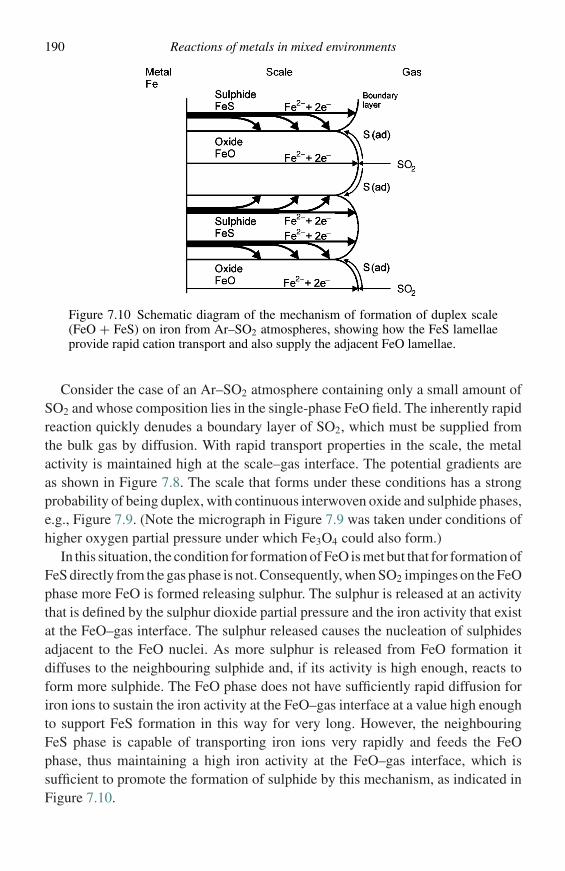
190 Reactions of metals in mixed environments
Figure 7.10 Schematic diagram of the mechanism of formation of duplex scale(FeO + FeS) on iron from Ar–SO2 atmospheres, showing how the FeS lamellaeprovide rapid cation transport and also supply the adjacent FeO lamellae.
Consider the case of an Ar–SO2 atmosphere containing only a small amount ofSO2 and whose composition lies in the single-phase FeO field. The inherently rapidreaction quickly denudes a boundary layer of SO2, which must be supplied fromthe bulk gas by diffusion. With rapid transport properties in the scale, the metalactivity is maintained high at the scale–gas interface. The potential gradients areas shown in Figure 7.8. The scale that forms under these conditions has a strongprobability of being duplex, with continuous interwoven oxide and sulphide phases,e.g., Figure 7.9. (Note the micrograph in Figure 7.9 was taken under conditions ofhigher oxygen partial pressure under which Fe3O4 could also form.)
In this situation, the condition for formation of FeO is met but that for formation ofFeS directly from the gas phase is not. Consequently, when SO2 impinges on the FeOphase more FeO is formed releasing sulphur. The sulphur is released at an activitythat is defined by the sulphur dioxide partial pressure and the iron activity that existat the FeO–gas interface. The sulphur released causes the nucleation of sulphidesadjacent to the FeO nuclei. As more sulphur is released from FeO formation itdiffuses to the neighbouring sulphide and, if its activity is high enough, reacts toform more sulphide. The FeO phase does not have sufficiently rapid diffusion foriron ions to sustain the iron activity at the FeO–gas interface at a value high enoughto support FeS formation in this way for very long. However, the neighbouringFeS phase is capable of transporting iron ions very rapidly and feeds the FeOphase, thus maintaining a high iron activity at the FeO–gas interface, which issufficient to promote the formation of sulphide by this mechanism, as indicated inFigure 7.10.
Conditions for sulphide formation 191
According to Figure 7.8, the sulphur dioxide potential is reduced to p′′SO2
at theFeO–gas interface. Thus, according to Equation (7.33b), the iron activity that mustbe maintained at the FeO–gas interface is given by Equation (7.34):
a′′Fe = 1
p′′1/(2n+m)SO2
exp
[1
(2n + m)RT
(2�Go
17 − �Go16 + �Go
18
)]. (7.34)
The data that are available for the Fe–O–S system are shown in Equations (7.35)and (7.36):
Fe + 1
2O2 = FeO �Go
35 = −264 176 + 64.7T J, (7.35)
Fe + 1
2S2 = FeS �Go
36 = −150 100 + 51.5T J. (7.36)
For example, at 800 ◦C, �Go35= −194753 J and replaces �Go
17, and �Go36=
−94841 J and replaces �Go18. Also, �Go
16= −279100 J. The stoichiometric factorsn and m are both unity. Thus, we have an activity expressed by Equation (7.37):
aFe >1
p′′1/3SO2
exp
[−204 925
3RT
]. (7.37)
For an experiment using Ar–1% SO2 the value of pSO2 in the bulk atmospheresis 0.01 atm and will be lower at the scale–gas interface. However, so long as theiron activity is held at a value greater than 2 × 10⁻³ the possibility exists for theformation of FeO and FeS at the scale–gas interface. Such a structure is shown inFigure 7.9,34 which corresponds to the diagrammatic Figure 7.10.
The development of a microstructure such as that in Figure 7.9 will now bedescribed in more detail. Consider the exposure of Fe in a gas corresponding to thecomposition marked ‘X’ in Figure 7.11. Initially Fe3O4 will form. However, thereaction will denude the atmosphere of oxygen in the region of the specimen surfaceresulting in a local change of atmosphere composition there to lower oxygen partialpressures. In atmospheres containing sulphur dioxide, this results in a local increasein sulphur partial pressure since the sulphur, oxygen, and sulphur dioxide partialpressures are related by the equilibrium constant given in Equation (7.16). Thus thegas composition at the scale–gas interface (or the metal surface in the early stages)follows the reaction path XYZ in Figure 7.11, entering the FeO field at point Y. Atthis stage the Fe3O4, formed earlier, is reduced to FeO and further reaction proceedsas described above with FeO forming and releasing sulphur into the boundary layerwhere the composition at the surface changes along the path YZ. On reaching pointZ, both FeO and FeS may form together as shown in Figure 7.10. Since SO2 isbeing consumed, the reaction path must cross the SO2 isobars which are shown asdashed diagonal lines in Figure 7.11. This represents the establishment of a SO2
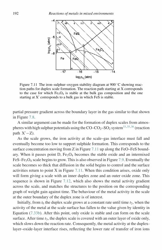
192 Reactions of metals in mixed environments
Figure 7.11 The iron–sulphur–oxygen stability diagram at 900 ◦C showing reac-tion paths for duplex scale formation. The reaction path starting at X correspondsto the case for which Fe3O4 is stable at the bulk gas composition and the onestarting at X′ corresponds to a bulk gas in which FeS is stable.
partial pressure gradient across the boundary layer in the gas similar to that shownin Figure 7.8.
A similar argument can be made for the formation of duplex scales from atmos-pheres with high sulphur potentials using the CO–CO2–SO2 system33,35,36 (reactionpath X′−Z).
As the scale grows, the iron activity at the scale–gas interface must fall andeventually become too low to support sulphide formation. This corresponds to thesurface concentration moving from Z in Figure 7.11 up along the FeO–FeS bound-ary. When it passes point D, Fe3O4 becomes the stable oxide and an intermixedFeS–Fe3O4 scale begins to grow. This is also observed in Figure 7.9. Eventually thescale becomes so thick that diffusion in the solid begins to control and the surfaceactivities return to point X in Figure 7.11. When this condition arises, oxide onlywill form giving a scale with an inner duplex zone and an outer oxide zone. Thissequence is shown in Figure 7.12, which also shows the metal activity gradientacross the scale, and matches the structures to the position on the correspondinggraph of weight gain against time. The behaviour of the metal activity in the scaleat the outer boundary of the duplex zone is of interest.
Initially, from t0 the duplex scale grows at a constant rate until time t2, when theactivity of the metal at the scale surface has fallen to the value given by identity inEquation (7.33b). After this point, only oxide is stable and can form on the scalesurface. After time t3, the duplex scale is covered with an outer layer of oxide only,which slows down the reaction rate. Consequently, the metal activity at the duplex-layer–oxide-layer interface rises, reflecting the lower rate of transfer of iron ions
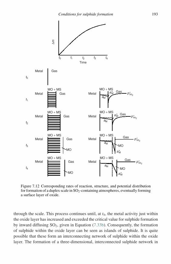
Conditions for sulphide formation 193
p°so2
p°so2
p°so2
p°so2
t0
t1
t2
t3
t4
∆mt0 t1 t2 t3 t4
Time
Metal
Metal
Metal
Metal
Metal Metal
Metal
Metal
Metal
Gas
GasGas
Gas
Gas
Gas
Gas
Gas
Gas
MO + MS
MO + MS
MO + MS
MO + MS MO + MS
MO + MS
MO + MS
MO + MS
MOMO
MOMO
aM
aM
aM
aM
a"M
a"M
a"M
a"M
Figure 7.12 Corresponding rates of reaction, structure, and potential distributionfor formation of a duplex scale in SO2-containing atmospheres, eventually forminga surface layer of oxide.
through the scale. This process continues until, at t4, the metal activity just withinthe oxide layer has increased and exceeded the critical value for sulphide formationby inward diffusing SO2, given in Equation (7.33b). Consequently, the formationof sulphide within the oxide layer can be seen as islands of sulphide. It is quitepossible that these form an interconnecting network of sulphide within the oxidelayer. The formation of a three-dimensional, interconnected sulphide network in
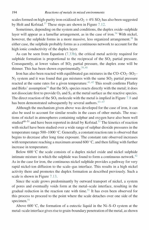
194 Reactions of metals in mixed environments
scales formed on high-purity iron oxidized in O2 + 4% SO2 has also been suggestedby Holt and Kofstad.37 These steps are shown in Figure 7.12.
Sometimes, depending on the system and conditions, the duplex oxide–sulphidelayer will appear as a lamellar arrangement, as in the case of iron.34 With nickel,however, the sulphide forms in a more massive, less organized arrangement.38 Ineither case, the sulphide probably forms as a continuous network to account for thehigh ionic conductivity of the duplex layer.
As can be seen from Equation (7.33b), the critical metal activity required forsulphide formation is proportional to the reciprocal of the SO2 partial pressure.Consequently, at lower values of SO2 partial pressure, the duplex zone will bethinner. This has been shown experimentally.39,40
Iron has also been reacted with equilibrated gas mixtures in the CO–CO2–SO2–N2 system and it was found that gas mixtures with the same SO2 partial pressurereacted at the same rates for a given temperature.41,42 This result confirms Flatleyand Birks’ assumption34 that the SO2 species reacts directly with the metal; it doesnot dissociate first to provide O2 and S2 at the metal surface as the reactive species.The direct reaction of the SO2 molecule with the metal is implied in Figure 7.8 andhas been demonstrated subsequently by several authors.43–47
Although the mechanism given above was developed for the case of iron, it canalso be used to account for similar results in the cases of other metals. The reac-tions of nickel in atmospheres containing sulphur and oxygen have also been wellstudied48–51 and have been reported in detail by Kofstad.53 The kinetics of reactionwith nickel have been studied over a wide range of sulphur dioxide pressures in thetemperature range 500–1000 ◦C. Generally, a constant reaction rate is observed thatbegins to decrease after long time exposure. The constant rate observed increaseswith temperature reaching a maximum around 600 ◦C, and then falling with furtherincrease in temperature.
Below 600 ◦C the scale consists of a duplex nickel oxide and nickel sulphideintimate mixture in which the sulphide was found to form a continuous network.42
As in the case for iron, the continuous nickel sulphide provides a pathway for veryrapid nickel-ion diffusion to the scale–gas interface. This results in a high nickelactivity there and promotes the duplex formation as described previously. Such ascale is shown in Figure 7.13.
Since the scale grows predominantly by outward transport of nickel, a systemof pores and eventually voids form at the metal–scale interface, resulting in thegradual reduction in the reaction rate with time.51 It has even been observed forthis process to proceed to the point where the scale detaches over one side of thespecimen.51
Above 600 ◦C, the formation of a eutectic liquid in the Ni–S–O system at themetal–scale interface gives rise to grain-boundary penetration of the metal, as shown
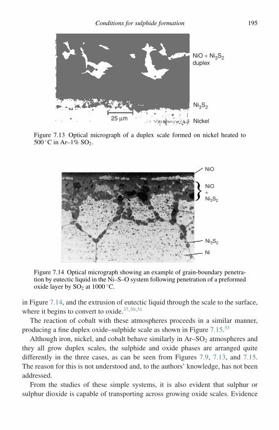
Conditions for sulphide formation 195
NiO + Ni3S2duplex
Ni3S2
Nickel25 µm
Figure 7.13 Optical micrograph of a duplex scale formed on nickel heated to500 ◦C in Ar–1% SO2.
NiO
Ni
NiO + Ni3S2
Ni3S2
Figure 7.14 Optical micrograph showing an example of grain-boundary penetra-tion by eutectic liquid in the Ni–S–O system following penetration of a preformedoxide layer by SO2 at 1000 ◦C.
in Figure 7.14, and the extrusion of eutectic liquid through the scale to the surface,where it begins to convert to oxide.37,50,51
The reaction of cobalt with these atmospheres proceeds in a similar manner,producing a fine duplex oxide–sulphide scale as shown in Figure 7.15.53
Although iron, nickel, and cobalt behave similarly in Ar–SO2 atmospheres andthey all grow duplex scales, the sulphide and oxide phases are arranged quitedifferently in the three cases, as can be seen from Figures 7.9, 7.13, and 7.15.The reason for this is not understood and, to the authors’ knowledge, has not beenaddressed.
From the studies of these simple systems, it is also evident that sulphur orsulphur dioxide is capable of transporting across growing oxide scales. Evidence
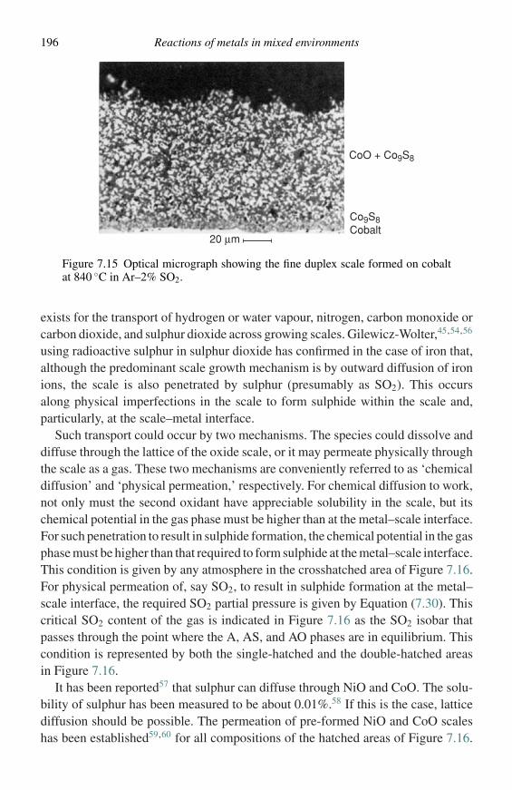
196 Reactions of metals in mixed environments
20 µm
Co9S8Cobalt
CoO + Co9S8
Figure 7.15 Optical micrograph showing the fine duplex scale formed on cobaltat 840 ◦C in Ar–2% SO2.
exists for the transport of hydrogen or water vapour, nitrogen, carbon monoxide orcarbon dioxide, and sulphur dioxide across growing scales. Gilewicz-Wolter,45,54,56
using radioactive sulphur in sulphur dioxide has confirmed in the case of iron that,although the predominant scale growth mechanism is by outward diffusion of ironions, the scale is also penetrated by sulphur (presumably as SO2). This occursalong physical imperfections in the scale to form sulphide within the scale and,particularly, at the scale–metal interface.
Such transport could occur by two mechanisms. The species could dissolve anddiffuse through the lattice of the oxide scale, or it may permeate physically throughthe scale as a gas. These two mechanisms are conveniently referred to as ‘chemicaldiffusion’ and ‘physical permeation,’ respectively. For chemical diffusion to work,not only must the second oxidant have appreciable solubility in the scale, but itschemical potential in the gas phase must be higher than at the metal–scale interface.For such penetration to result in sulphide formation, the chemical potential in the gasphase must be higher than that required to form sulphide at the metal–scale interface.This condition is given by any atmosphere in the crosshatched area of Figure 7.16.For physical permeation of, say SO2, to result in sulphide formation at the metal–scale interface, the required SO2 partial pressure is given by Equation (7.30). Thiscritical SO2 content of the gas is indicated in Figure 7.16 as the SO2 isobar thatpasses through the point where the A, AS, and AO phases are in equilibrium. Thiscondition is represented by both the single-hatched and the double-hatched areasin Figure 7.16.
It has been reported57 that sulphur can diffuse through NiO and CoO. The solu-bility of sulphur has been measured to be about 0.01%.58 If this is the case, latticediffusion should be possible. The permeation of pre-formed NiO and CoO scaleshas been established59,60 for all compositions of the hatched areas of Figure 7.16.
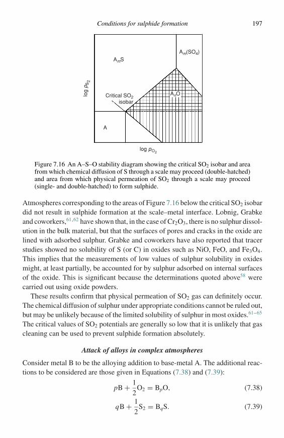
Conditions for sulphide formation 197
AmSAm(SO4)
AnO
log pO2
log
p s2
A
Critical SO2isobar
Figure 7.16 An A–S–O stability diagram showing the critical SO2 isobar and areafrom which chemical diffusion of S through a scale may proceed (double-hatched)and area from which physical permeation of SO2 through a scale may proceed(single- and double-hatched) to form sulphide.
Atmospheres corresponding to the areas of Figure 7.16 below the critical SO2 isobardid not result in sulphide formation at the scale–metal interface. Lobnig, Grabkeand coworkers,61,62 have shown that, in the case of Cr2O3, there is no sulphur dissol-ution in the bulk material, but that the surfaces of pores and cracks in the oxide arelined with adsorbed sulphur. Grabke and coworkers have also reported that tracerstudies showed no solubility of S (or C) in oxides such as NiO, FeO, and Fe3O4.This implies that the measurements of low values of sulphur solubility in oxidesmight, at least partially, be accounted for by sulphur adsorbed on internal surfacesof the oxide. This is significant because the determinations quoted above58 werecarried out using oxide powders.
These results confirm that physical permeation of SO2 gas can definitely occur.The chemical diffusion of sulphur under appropriate conditions cannot be ruled out,but may be unlikely because of the limited solubility of sulphur in most oxides.61–65
The critical values of SO2 potentials are generally so low that it is unlikely that gascleaning can be used to prevent sulphide formation absolutely.
Attack of alloys in complex atmospheres
Consider metal B to be the alloying addition to base-metal A. The additional reac-tions to be considered are those given in Equations (7.38) and (7.39):
pB + 1
2O2 = BpO, (7.38)
qB + 1
2S2 = BqS. (7.39)
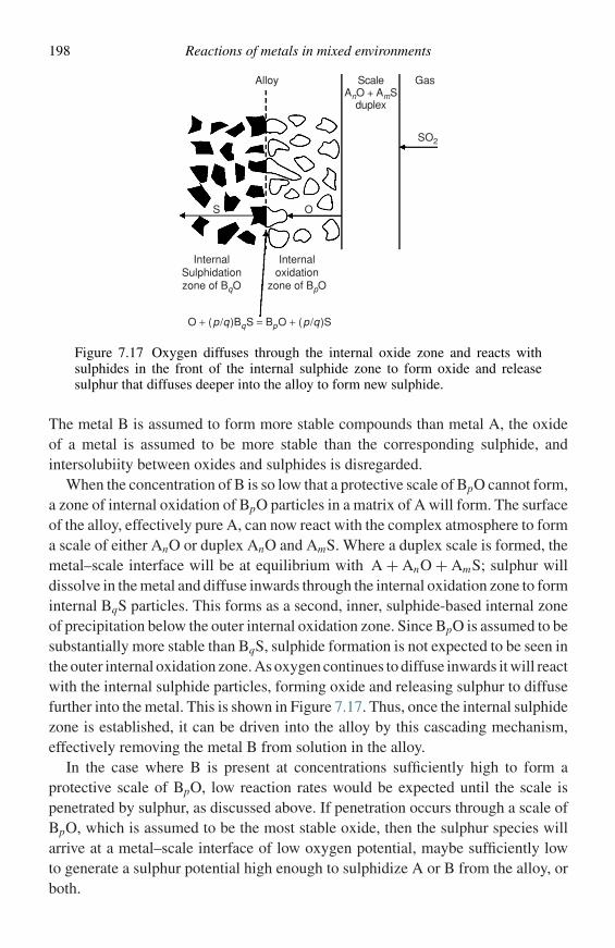
198 Reactions of metals in mixed environments
Alloy
S O
O + (p/q)BqS = BpO + (p/q)S
Internaloxidation
zone of BpO
InternalSulphidationzone of BqO
Gas
SO2
ScaleAnO + AmS
duplex
Figure 7.17 Oxygen diffuses through the internal oxide zone and reacts withsulphides in the front of the internal sulphide zone to form oxide and releasesulphur that diffuses deeper into the alloy to form new sulphide.
The metal B is assumed to form more stable compounds than metal A, the oxideof a metal is assumed to be more stable than the corresponding sulphide, andintersolubiity between oxides and sulphides is disregarded.
When the concentration of B is so low that a protective scale of BpO cannot form,a zone of internal oxidation of BpO particles in a matrix of A will form. The surfaceof the alloy, effectively pure A, can now react with the complex atmosphere to forma scale of either AnO or duplex AnO and AmS. Where a duplex scale is formed, themetal–scale interface will be at equilibrium with A + AnO + AmS; sulphur willdissolve in the metal and diffuse inwards through the internal oxidation zone to forminternal BqS particles. This forms as a second, inner, sulphide-based internal zoneof precipitation below the outer internal oxidation zone. Since BpO is assumed to besubstantially more stable than BqS, sulphide formation is not expected to be seen inthe outer internal oxidation zone. As oxygen continues to diffuse inwards it will reactwith the internal sulphide particles, forming oxide and releasing sulphur to diffusefurther into the metal. This is shown in Figure 7.17. Thus, once the internal sulphidezone is established, it can be driven into the alloy by this cascading mechanism,effectively removing the metal B from solution in the alloy.
In the case where B is present at concentrations sufficiently high to form aprotective scale of BpO, low reaction rates would be expected until the scale ispenetrated by sulphur, as discussed above. If penetration occurs through a scale ofBpO, which is assumed to be the most stable oxide, then the sulphur species willarrive at a metal–scale interface of low oxygen potential, maybe sufficiently lowto generate a sulphur potential high enough to sulphidize A or B from the alloy, orboth.
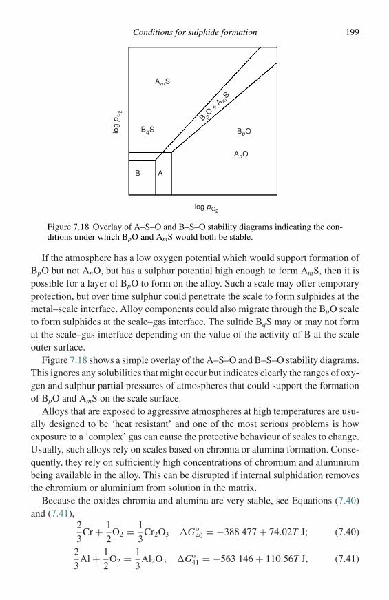
Conditions for sulphide formation 199
AmS
BqS
B pO +
A mS
AnO
A
log pO2
log
pS
2
B
BpO
Figure 7.18 Overlay of A–S–O and B–S–O stability diagrams indicating the con-ditions under which BpO and AmS would both be stable.
If the atmosphere has a low oxygen potential which would support formation ofBpO but not AnO, but has a sulphur potential high enough to form AmS, then it ispossible for a layer of BpO to form on the alloy. Such a scale may offer temporaryprotection, but over time sulphur could penetrate the scale to form sulphides at themetal–scale interface. Alloy components could also migrate through the BpO scaleto form sulphides at the scale–gas interface. The sulfide BqS may or may not format the scale–gas interface depending on the value of the activity of B at the scaleouter surface.
Figure 7.18 shows a simple overlay of the A–S–O and B–S–O stability diagrams.This ignores any solubilities that might occur but indicates clearly the ranges of oxy-gen and sulphur partial pressures of atmospheres that could support the formationof BpO and AmS on the scale surface.
Alloys that are exposed to aggressive atmospheres at high temperatures are usu-ally designed to be ‘heat resistant’ and one of the most serious problems is howexposure to a ‘complex’ gas can cause the protective behaviour of scales to change.Usually, such alloys rely on scales based on chromia or alumina formation. Conse-quently, they rely on sufficiently high concentrations of chromium and aluminiumbeing available in the alloy. This can be disrupted if internal sulphidation removesthe chromium or aluminium from solution in the matrix.
Because the oxides chromia and alumina are very stable, see Equations (7.40)and (7.41),
2
3Cr + 1
2O2 = 1
3Cr2O3 �Go
40 = −388 477 + 74.02T J; (7.40)
2
3Al + 1
2O2 = 1
3Al2O3 �Go
41 = −563 146 + 110.56T J, (7.41)
200 Reactions of metals in mixed environments
the oxygen partial pressures imposed at the scale–metal interface will be low andare given by Equation (7.42):
pO2 = 1
a4/3M
exp
(2�Go
RT
). (7.42)
At 1100 K, this gives values of 10−29 atm for a chromium activity of 0.2 and10−41 atm for an aluminium activity of 0.06. Such low oxygen potentials are capableof generating very high sulphur potentials at the scale–metal interface. Of courseequilibrium pressures will not be realized because the sulphur will be consumed byforming sulphides of other alloy components. If the sulphur dioxide penetration isslow, it may be consumed as quickly as it arrives and only the most stable sulphidescould be found to form initially.
It is possible that the sulphide formed in this way may form a zone of internalsulphidation rather than a complete layer at the scale–metal interface. This wouldremove the chromium and aluminium from solution in the matrix and leave thesystem open for the formation of rapidly growing sulphides of metals such as iron,nickel, or cobalt.
Of course, if the protective scale of chromia or alumina is not penetrated bySO2, sulphide cannot form at the scale–metal interface. This was found9 forNi–20 wt% Cr, Co–35 wt% Cr and Fe–35 wt% Cr alloys exposed to pure SO2
at 900 ◦C and emphasizes the resistance of a chromia scale to permeation. On theother hand, alloys in the Fe–Cr–Al, Ni–Cr–Al and Co–Cr–Al systems were exposedto atmospheres in the H2–H2S–H2O system. These atmospheres had compositionsthat supported the formation of chromia or alumina together with the sulphides ofFe, Ni and Co at the scale–metal interface.9,66 In these cases, a protective layerof chromia or alumina that formed initially was penetrated by sulphur to formiron, nickel, and cobalt sulphides at the scale–metal interface. Furthermore, iron,nickel, and cobalt ions apparently diffused through the oxide layer to form theirsulphides on the outside of the protective scale. Thus the original protective scalewas sandwiched between base-metal sulphides.
It was established40,66–69 that pre-oxidation in a sulphur-free environment doesnot completely prevent sulphur penetration on subsequent exposure to an atmos-phere containing sulphur. This is evident from the edges and corners of the structure,confirming that mechanical factors play a role in the breakdown. Xu et al. 67 foundthat such penetration of a protective oxide scale by sulphur resulted in its eventualbreakdown and the onset of rapid reaction kinetics. These mechanisms appear tobe responsible for the deterioration of alloys that form chromia protective layersand that are used in atmospheres of high sulphur potential.70
In fact, the permeation of protective scales is not limited to sulphurous species.This has been demonstrated by Zheng and Young,43 who exposed Fe–28 wt% Cr,
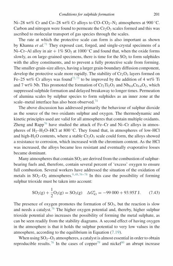
Conditions for sulphide formation 201
Ni–28 wt% Cr and Co–28 wt% Cr alloys to CO–CO2–N2 atmospheres at 900 ◦C.Carbon and nitrogen were found to permeate the Cr2O3 scales formed and this wasascribed to molecular transport of gas species through the scales.
The rate at which the protective scale can form is also important as shownby Khanna et al.71 They exposed cast, forged, and single-crystal specimens of aNi–Cr–Al alloy in air + 1% SO2 at 1000 ◦C and found that, when the oxide formsslowly, as on large-grained specimens, there is time for the SO2 to form sulphideswith the alloy constituents, and to prevent a fully protective scale from forming.The smaller-grain-size alloys, having a larger grain-boundary diffusion component,develop the protective scale more rapidly. The stability of Cr2O3 layers formed onFe–25 wt% Cr alloys was found72,73 to be improved by the addition of 4 wt% Tiand 7 wt% Nb. This promoted the formation of Cr2Ti2O2 and Nb0.6Cr0.4O2, whichsuppressed sulphide formation and delayed breakaway to longer times. Permeationof alumina scales by sulphur species to form sulphides as an inner zone at thescale–metal interface has also been observed.74
The above discussion has addressed primarily the behaviour of sulphur dioxideas the source of the two oxidants sulphur and oxygen. The thermodynamic andkinetic principles used are valid for all atmospheres that contain multiple oxidants.Zheng and Rapp76 have studied the attack of Fe–Cr and Ni–Cr alloys in atmos-pheres of H2–H2O–HCl at 800 ◦C. They found that, in atmospheres of low-HCland high-H2O contents, where a stable Cr2O3 scale could form, the alloys showeda resistance to corrosion, which increased with the chromium content. As the HClwas increased, the alloys became less resistant and eventually evaporative lossesbecame dominant.
Many atmospheres that contain SO2 are derived from the combustion of sulphur-bearing fuels and, therefore, contain several percent of ‘excess’ oxygen to ensurefull combustion. Several workers have addressed the situation of the oxidation ofmetals in SO2–O2 atmospheres.9,48,76–78 In this case the possibility of formingsulphur trioxide must be taken into account:
SO2(g) + 1
2O2(g) = SO3(g) �Go
43 = −99 000 + 93.95T J. (7.43)
The presence of oxygen promotes the formation of SO3, but the reaction is slowand needs a catalyst.76 The higher oxygen potential and, thereby, higher sulphurtrioxide potential also increases the possibility of forming the metal sulphate, ascan be seen readily from the stability diagrams. A second effect of having oxygenin the atmosphere is that it holds the sulphur potential to very low values in theatmosphere, according to the equilibrium in Equation (7.19).
When using SO2–O2 atmospheres, a catalyst is almost essential in order to obtainreproducible results.76 In the cases of copper79 and nickel80 an abrupt increase
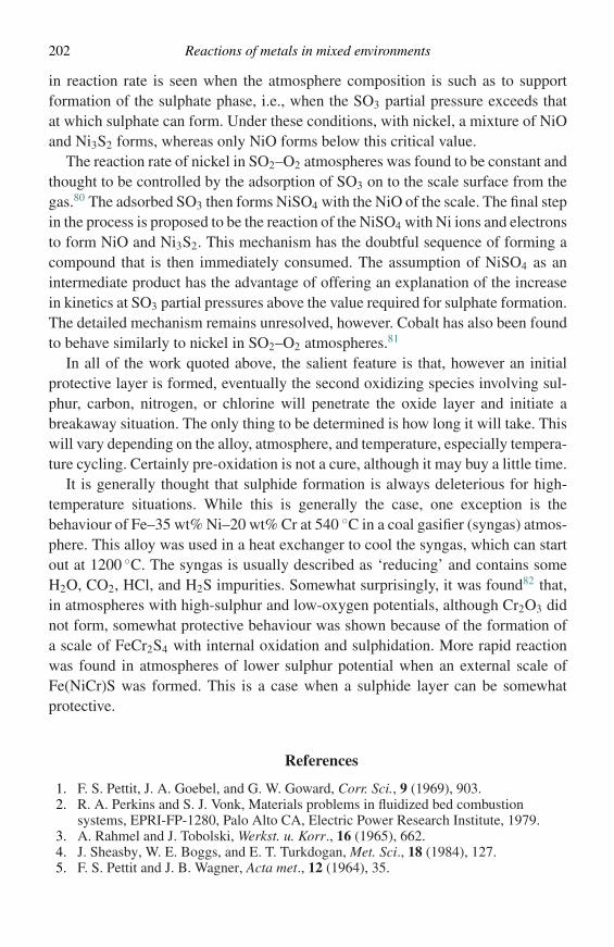
202 Reactions of metals in mixed environments
in reaction rate is seen when the atmosphere composition is such as to supportformation of the sulphate phase, i.e., when the SO3 partial pressure exceeds thatat which sulphate can form. Under these conditions, with nickel, a mixture of NiOand Ni3S2 forms, whereas only NiO forms below this critical value.
The reaction rate of nickel in SO2–O2 atmospheres was found to be constant andthought to be controlled by the adsorption of SO3 on to the scale surface from thegas.80 The adsorbed SO3 then forms NiSO4 with the NiO of the scale. The final stepin the process is proposed to be the reaction of the NiSO4 with Ni ions and electronsto form NiO and Ni3S2. This mechanism has the doubtful sequence of forming acompound that is then immediately consumed. The assumption of NiSO4 as anintermediate product has the advantage of offering an explanation of the increasein kinetics at SO3 partial pressures above the value required for sulphate formation.The detailed mechanism remains unresolved, however. Cobalt has also been foundto behave similarly to nickel in SO2–O2 atmospheres.81
In all of the work quoted above, the salient feature is that, however an initialprotective layer is formed, eventually the second oxidizing species involving sul-phur, carbon, nitrogen, or chlorine will penetrate the oxide layer and initiate abreakaway situation. The only thing to be determined is how long it will take. Thiswill vary depending on the alloy, atmosphere, and temperature, especially tempera-ture cycling. Certainly pre-oxidation is not a cure, although it may buy a little time.
It is generally thought that sulphide formation is always deleterious for high-temperature situations. While this is generally the case, one exception is thebehaviour of Fe–35 wt% Ni–20 wt% Cr at 540 ◦C in a coal gasifier (syngas) atmos-phere. This alloy was used in a heat exchanger to cool the syngas, which can startout at 1200 ◦C. The syngas is usually described as ‘reducing’ and contains someH2O, CO2, HCl, and H2S impurities. Somewhat surprisingly, it was found82 that,in atmospheres with high-sulphur and low-oxygen potentials, although Cr2O3 didnot form, somewhat protective behaviour was shown because of the formation ofa scale of FeCr2S4 with internal oxidation and sulphidation. More rapid reactionwas found in atmospheres of lower sulphur potential when an external scale ofFe(NiCr)S was formed. This is a case when a sulphide layer can be somewhatprotective.
References
1. F. S. Pettit, J. A. Goebel, and G. W. Goward, Corr. Sci., 9 (1969), 903.2. R. A. Perkins and S. J. Vonk, Materials problems in fluidized bed combustion
systems, EPRI-FP-1280, Palo Alto CA, Electric Power Research Institute, 1979.3. A. Rahmel and J. Tobolski, Werkst. u. Korr., 16 (1965), 662.4. J. Sheasby, W. E. Boggs, and E. T. Turkdogan, Met. Sci., 18 (1984), 127.5. F. S. Pettit and J. B. Wagner, Acta met., 12 (1964), 35.
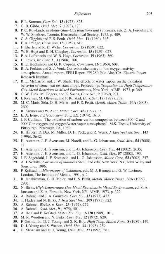
References 203
6. P. L. Surman, Corr. Sci., 13 (1973), 825.7. G. B. Gibbs, Oxid. Met., 7 (1973), 173.8. P. C. Rowlands, in Metal–Slag–Gas Reactions and Processes, eds. Z. A. Foroulis and
W. W. Smeltzer, Toronto, Electrochemical Society, 1975, p. 409.9. C. S. Giggins and F. S. Pettit, Oxid. Met., 14 (1980), 363.
10. F. A. Prange, Corrosion, 15 (1959), 619.11. F. Eberle and R. D. Wylie, Corrosion, 15 (1959), 622.12. W. B. Hoyt and R. H. Caughey, Corrosion, 15 (1959), 627.13. P. A. Lefrancois and W. B. Hoyt, Corrosion, 19 (1963), 360.14. H. Lewis, Br. Corr. J., 3 (1968), 166.15. B. E. Hopkinson and G. R. Copson, Corrosion, 16 (1960), 608.16. R. A. Perkins and S. J. Vonk, Corrosion chemistry in low oxygen activity
atmospheres. Annual report, EPRI Report FP1280 Palo Alto, CA, Electric PowerResearch Institute.
17. R. L. McCarron and. J. W. Shulz, The effects of water vapour on the oxidationbehavior of some heat resistant alloys. Proceedings Symposium on High TemperatureGas–Metal Reactions in Mixed Environments, New York, AIME, 1973, p. 360.
18. C. W. Tuck, M. Odgers, and K. Sachs, Corr. Sci., 9 (1969), 271.19. I. Kvernes, M. Oliveira, and P. Kofstad, Corr. Sci., 17 (1977), 237.20. M. C. Maris-Sida, G. H. Meier, and F. S. Pettit, Metall. Mater. Trans., 34A (2003),
2609.21. R. Kremer and W. Auer, Mater. Corr., 48 (1997), 35.22. E. A. Irene, J. Electrochem. Soc., 121 (1974), 1613.23. J. F. Cullinan, ‘The oxidation of carbon–carbon composites between 300 ◦C and
900 ◦C in oxygen and oxygen/water vapor atmospheres’, M.S. Thesis, University ofPittsburgh, Pittsburgh, PA, 1989.
24. K. Hilpert, D. Das, M. Miller, D. H. Peck, and R. Weiss, J. Electrochem. Soc., 143(1996), 3642.
25. H. Asteman, J.-E. Svensson, M. Norell, and L.-G. Johansson, Oxid. Met., 54 (2000),11.
26. H. Asteman, J.-E. Svensson, and L.-G. Johansson, Corr. Sci., 44 (2002), 2635.27. H. Asteman, J.-E. Svensson, and L.-G. Johansson, Oxid. Met., 57 (2002), 193.28. J. E. Segerdahl, J.-E. Svensson, and L.-G. Johansson, Mater. Corr., 53 (2002), 247.29. A. J. Sedriks, Corrosion of Stainless Steel, 2nd edn, New York, NY, John Wiley and
Sons, Inc., 1996.30. P. Kofstad, in Microscopy of Oxidation, eds. M. J. Bennett and G. W. Lorimer,
London, The Institute of Metals, 1991, p. 2.31. R. Janakiraman, G. H. Meier, and F. S. Pettit, Metall. Mater. Trans., 30A (1999),
2905.32. N. Birks, High Temperature Gas-Metal Reactions in Mixed Environment, ed. S. A.
Jansson and Z. A. Foroulis, New York, NY, AIME, 1973, p. 322.33. A. Rahmel and J. A. Gonzales, Corr. Sci., 13 (1973), 433.34. T. Flatley and N. Birks, J. Iron Steel Inst., 209 (1971), 523.35. A. Rahmel, Werkst. u. Korr., 23 (1972), 272.36. A. Rahmel, Oxid. Met., 9 (1975), 401.37. A. Holt and P. Kofstad, Mater. Sci. Eng., A120 (1989), 101.38. M. R. Wootton and N. Birks, Corr. Sci., 12 (1972), 829.39. F. Gesmundo, D. J. Young, and S. K. Roy, High Temp. Mater. Proc., 8 (1989), 149.40. D. J. Young and S. Watson, Oxid. Met., 44 (1995), 239.41. G. McAdam and D. J. Young, Oxid. Met., 37 (1992), 281.
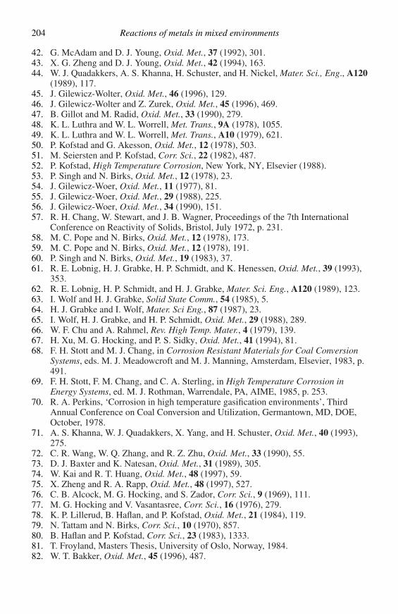
204 Reactions of metals in mixed environments
42. G. McAdam and D. J. Young, Oxid. Met., 37 (1992), 301.43. X. G. Zheng and D. J. Young, Oxid. Met., 42 (1994), 163.44. W. J. Quadakkers, A. S. Khanna, H. Schuster, and H. Nickel, Mater. Sci., Eng., A120
(1989), 117.45. J. Gilewicz-Wolter, Oxid. Met., 46 (1996), 129.46. J. Gilewicz-Wolter and Z. Zurek, Oxid. Met., 45 (1996), 469.47. B. Gillot and M. Radid, Oxid. Met., 33 (1990), 279.48. K. L. Luthra and W. L. Worrell, Met. Trans., 9A (1978), 1055.49. K. L. Luthra and W. L. Worrell, Met. Trans., A10 (1979), 621.50. P. Kofstad and G. Akesson, Oxid. Met., 12 (1978), 503.51. M. Seiersten and P. Kofstad, Corr. Sci., 22 (1982), 487.52. P. Kofstad, High Temperature Corrosion, New York, NY, Elsevier (1988).53. P. Singh and N. Birks, Oxid. Met., 12 (1978), 23.54. J. Gilewicz-Woer, Oxid. Met., 11 (1977), 81.55. J. Gilewicz-Woer, Oxid. Met., 29 (1988), 225.56. J. Gilewicz-Woer, Oxid. Met., 34 (1990), 151.57. R. H. Chang, W. Stewart, and J. B. Wagner, Proceedings of the 7th International
Conference on Reactivity of Solids, Bristol, July 1972, p. 231.58. M. C. Pope and N. Birks, Oxid. Met., 12 (1978), 173.59. M. C. Pope and N. Birks, Oxid. Met., 12 (1978), 191.60. P. Singh and N. Birks, Oxid. Met., 19 (1983), 37.61. R. E. Lobnig, H. J. Grabke, H. P. Schmidt, and K. Henessen, Oxid. Met., 39 (1993),
353.62. R. E. Lobnig, H. P. Schmidt, and H. J. Grabke, Mater. Sci. Eng., A120 (1989), 123.63. I. Wolf and H. J. Grabke, Solid State Comm., 54 (1985), 5.64. H. J. Grabke and I. Wolf, Mater. Sci Eng., 87 (1987), 23.65. I. Wolf, H. J. Grabke, and H. P. Schmidt, Oxid. Met., 29 (1988), 289.66. W. F. Chu and A. Rahmel, Rev. High Temp. Mater., 4 (1979), 139.67. H. Xu, M. G. Hocking, and P. S. Sidky, Oxid. Met., 41 (1994), 81.68. F. H. Stott and M. J. Chang, in Corrosion Resistant Materials for Coal Conversion
Systems, eds. M. J. Meadowcroft and M. J. Manning, Amsterdam, Elsevier, 1983, p.491.
69. F. H. Stott, F. M. Chang, and C. A. Sterling, in High Temperature Corrosion inEnergy Systems, ed. M. J. Rothman, Warrendale, PA, AIME, 1985, p. 253.
70. R. A. Perkins, ‘Corrosion in high temperature gasification environments’, ThirdAnnual Conference on Coal Conversion and Utilization, Germantown, MD, DOE,October, 1978.
71. A. S. Khanna, W. J. Quadakkers, X. Yang, and H. Schuster, Oxid. Met., 40 (1993),275.
72. C. R. Wang, W. Q. Zhang, and R. Z. Zhu, Oxid. Met., 33 (1990), 55.73. D. J. Baxter and K. Natesan, Oxid. Met., 31 (1989), 305.74. W. Kai and R. T. Huang, Oxid. Met., 48 (1997), 59.75. X. Zheng and R. A. Rapp, Oxid. Met., 48 (1997), 527.76. C. B. Alcock, M. G. Hocking, and S. Zador, Corr. Sci., 9 (1969), 111.77. M. G. Hocking and V. Vasantasree, Corr. Sci., 16 (1976), 279.78. K. P. Lillerud, B. Haflan, and P. Kofstad, Oxid. Met., 21 (1984), 119.79. N. Tattam and N. Birks, Corr. Sci., 10 (1970), 857.80. B. Haflan and P. Kofstad, Corr. Sci., 23 (1983), 1333.81. T. Froyland, Masters Thesis, University of Oslo, Norway, 1984.82. W. T. Bakker, Oxid. Met., 45 (1996), 487.
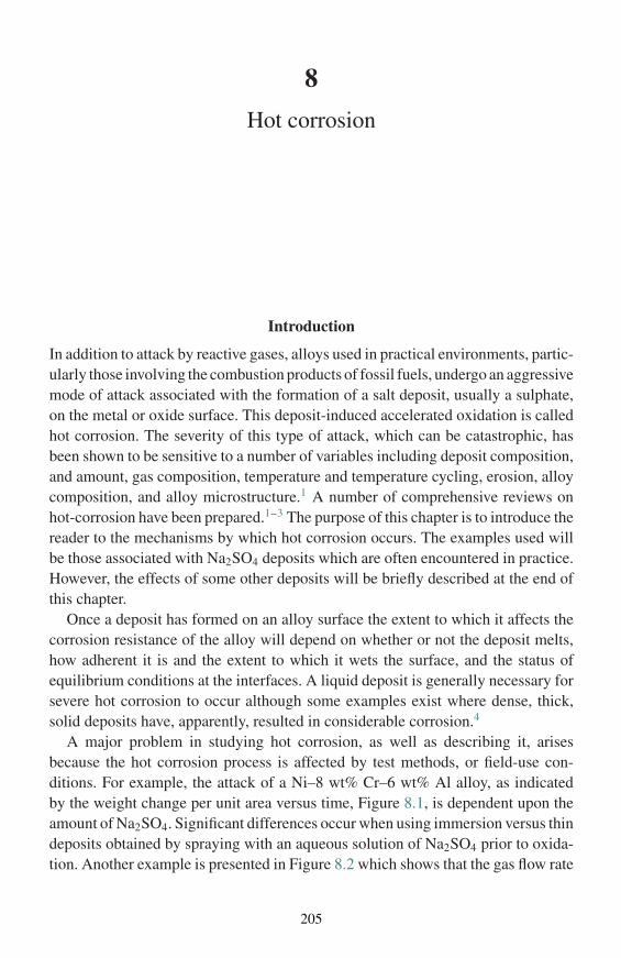
8
Hot corrosion
Introduction
In addition to attack by reactive gases, alloys used in practical environments, partic-ularly those involving the combustion products of fossil fuels, undergo an aggressivemode of attack associated with the formation of a salt deposit, usually a sulphate,on the metal or oxide surface. This deposit-induced accelerated oxidation is calledhot corrosion. The severity of this type of attack, which can be catastrophic, hasbeen shown to be sensitive to a number of variables including deposit composition,and amount, gas composition, temperature and temperature cycling, erosion, alloycomposition, and alloy microstructure.1 A number of comprehensive reviews onhot-corrosion have been prepared.1–3 The purpose of this chapter is to introduce thereader to the mechanisms by which hot corrosion occurs. The examples used willbe those associated with Na2SO4 deposits which are often encountered in practice.However, the effects of some other deposits will be briefly described at the end ofthis chapter.
Once a deposit has formed on an alloy surface the extent to which it affects thecorrosion resistance of the alloy will depend on whether or not the deposit melts,how adherent it is and the extent to which it wets the surface, and the status ofequilibrium conditions at the interfaces. A liquid deposit is generally necessary forsevere hot corrosion to occur although some examples exist where dense, thick,solid deposits have, apparently, resulted in considerable corrosion.4
A major problem in studying hot corrosion, as well as describing it, arisesbecause the hot corrosion process is affected by test methods, or field-use con-ditions. For example, the attack of a Ni–8 wt% Cr–6 wt% Al alloy, as indicatedby the weight change per unit area versus time, Figure 8.1, is dependent upon theamount of Na2SO4. Significant differences occur when using immersion versus thindeposits obtained by spraying with an aqueous solution of Na2SO4 prior to oxida-tion. Another example is presented in Figure 8.2 which shows that the gas flow rate
205
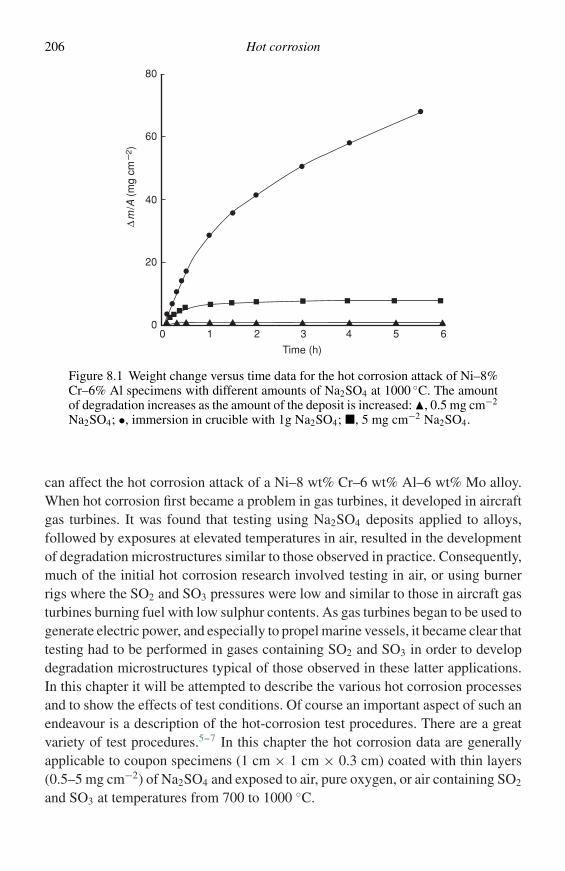
206 Hot corrosion
Time (h)
00
20
40
60
80
1 2 3 4 5 6
∆m
/A (
mg
cm−2
)
Figure 8.1 Weight change versus time data for the hot corrosion attack of Ni–8%Cr–6% Al specimens with different amounts of Na2SO4 at 1000 ◦C. The amountof degradation increases as the amount of the deposit is increased: �, 0.5 mg cm−2
Na2SO4; •, immersion in crucible with 1g Na2SO4; �, 5 mg cm−2 Na2SO4.
can affect the hot corrosion attack of a Ni–8 wt% Cr–6 wt% Al–6 wt% Mo alloy.When hot corrosion first became a problem in gas turbines, it developed in aircraftgas turbines. It was found that testing using Na2SO4 deposits applied to alloys,followed by exposures at elevated temperatures in air, resulted in the developmentof degradation microstructures similar to those observed in practice. Consequently,much of the initial hot corrosion research involved testing in air, or using burnerrigs where the SO2 and SO3 pressures were low and similar to those in aircraft gasturbines burning fuel with low sulphur contents. As gas turbines began to be used togenerate electric power, and especially to propel marine vessels, it became clear thattesting had to be performed in gases containing SO2 and SO3 in order to developdegradation microstructures typical of those observed in these latter applications.In this chapter it will be attempted to describe the various hot corrosion processesand to show the effects of test conditions. Of course an important aspect of such anendeavour is a description of the hot-corrosion test procedures. There are a greatvariety of test procedures.5–7 In this chapter the hot corrosion data are generallyapplicable to coupon specimens (1 cm × 1 cm × 0.3 cm) coated with thin layers(0.5–5 mg cm−2) of Na2SO4 and exposed to air, pure oxygen, or air containing SO2
and SO3 at temperatures from 700 to 1000 ◦C.
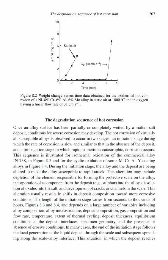
The degradation sequence of hot corrosion 207
10
8
6
4
2
00 2 4 6 8 10
Time (min)
∆m
/A (
mg
cm−2
)
Static air
O2 (31cm s−1)
Figure 8.2 Weight change versus time data obtained for the isothermal hot cor-rosion of a Ni–8% Cr–6% Al–6% Mo alloy in static air at 1000 ◦C and in oxygenhaving a linear flow rate of 31 cm s−1.
The degradation sequence of hot corrosion
Once an alloy surface has been partially or completely wetted by a molten saltdeposit, conditions for severe corrosion may develop. The hot corrosion of virtuallyall susceptible alloys is observed to occur in two stages: an initiation stage duringwhich the rate of corrosion is slow and similar to that in the absence of the deposit,and a propagation stage in which rapid, sometimes catastrophic, corrosion occurs.This sequence is illustrated for isothermal oxidation of the commercial alloyIN-738, in Figure 8.3 and for the cyclic oxidation of some M–Cr–Al–Y coatingalloys in Figure 8.4. During the initiation stage, the alloy and the deposit are beingaltered to make the alloy susceptible to rapid attack. This alteration may includedepletion of the element responsible for forming the protective scale on the alloy,incorporation of a component from the deposit (e.g., sulphur) into the alloy, dissolu-tion of oxides into the salt, and development of cracks or channels in the scale. Thisalteration usually results in shifts in deposit composition toward more corrosiveconditions. The length of the initiation stage varies from seconds to thousands ofhours, Figures 8.3 and 8.4, and depends on a large number of variables includingalloy composition, alloy microstructure, deposit composition, gas composition andflow rate, temperature, extent of thermal cycling, deposit thickness, equilibriumconditions at the deposit interfaces, specimen geometry, and the presence orabsence of erosive conditions. In many cases, the end of the initiation stage followsthe local penetration of the liquid deposit through the scale and subsequent spread-ing along the scale–alloy interface. This situation, in which the deposit reaches
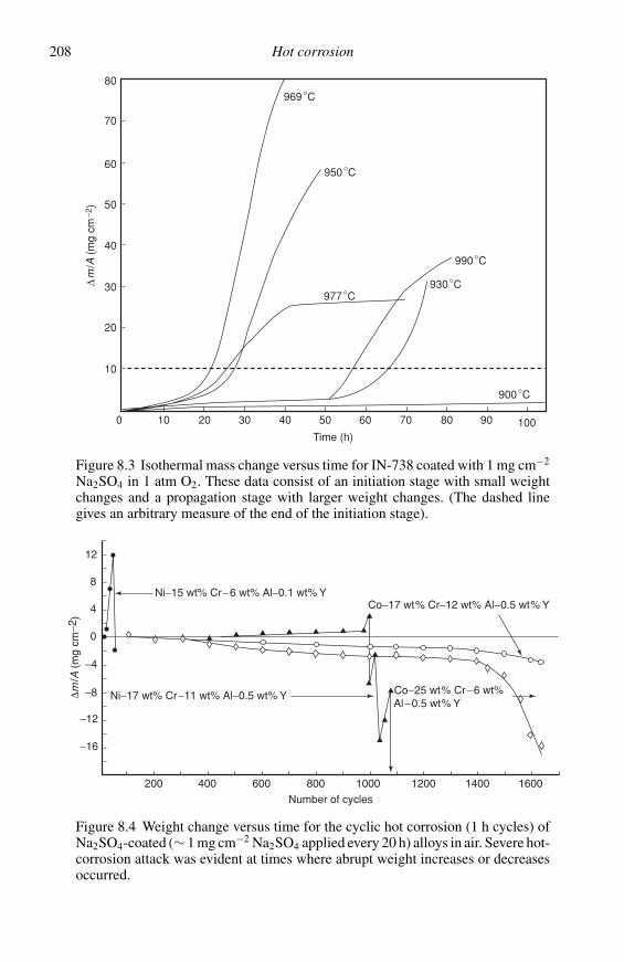
208 Hot corrosion
80
70
60
50
40
30
20
10
0 10 20 30 40 50 60 70 80 90 100
900°C
930°C
990°C
977°C
950°C
969°C
Time (h)
∆m
/A (
mg
cm−2
)
Figure 8.3 Isothermal mass change versus time for IN-738 coated with 1 mg cm−2
Na2SO4 in 1 atm O2. These data consist of an initiation stage with small weightchanges and a propagation stage with larger weight changes. (The dashed linegives an arbitrary measure of the end of the initiation stage).
12
8
4
0
−4
−8
−12
−16
200 400 600 800 1000 1200 1400 1600
Number of cycles
∆m/A
(m
g cm
−2)
Ni−15 wt% Cr−6 wt% Al−0.1 wt% Y
Ni−17 wt% Cr−11 wt% Al−0.5 wt% Y Co−25 wt% Cr−6 wt%
Co−17 wt% Cr−12 wt% Al−0.5 wt% Y
Al−0.5 wt% Y
Figure 8.4 Weight change versus time for the cyclic hot corrosion (1 h cycles) ofNa2SO4-coated (∼ 1 mg cm−2 Na2SO4 applied every 20 h) alloys in air. Severe hot-corrosion attack was evident at times where abrupt weight increases or decreasesoccurred.
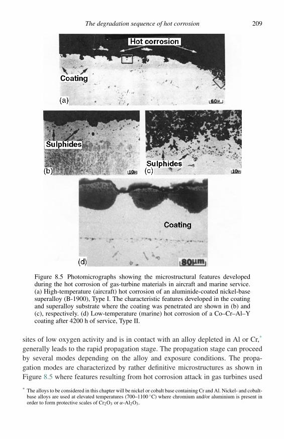
The degradation sequence of hot corrosion 209
Figure 8.5 Photomicrographs showing the microstructural features developedduring the hot corrosion of gas-turbine materials in aircraft and marine service.(a) High-temperature (aircraft) hot corrosion of an aluminide-coated nickel-basesuperalloy (B-1900), Type I. The characteristic features developed in the coatingand superalloy substrate where the coating was penetrated are shown in (b) and(c), respectively. (d) Low-temperature (marine) hot corrosion of a Co–Cr–Al–Ycoating after 4200 h of service, Type II.
sites of low oxygen activity and is in contact with an alloy depleted in Al or Cr,*
generally leads to the rapid propagation stage. The propagation stage can proceedby several modes depending on the alloy and exposure conditions. The propa-gation modes are characterized by rather definitive microstructures as shown inFigure 8.5 where features resulting from hot corrosion attack in gas turbines used
* The alloys to be considered in this chapter will be nickel or cobalt base containing Cr and Al. Nickel- and cobalt-base alloys are used at elevated temperatures (700–1100 ◦C) where chromium and/or aluminium is present inorder to form protective scales of Cr2O3 or α-Al2O3.
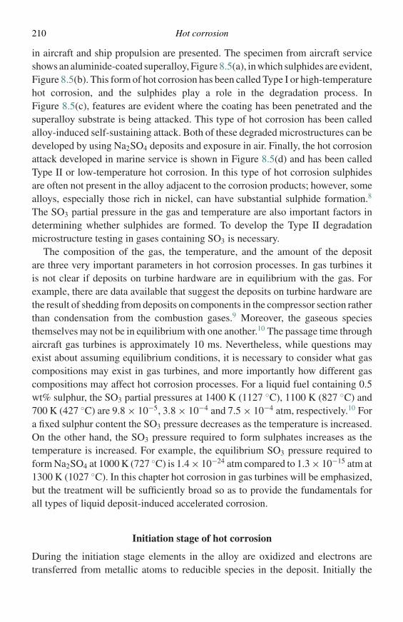
210 Hot corrosion
in aircraft and ship propulsion are presented. The specimen from aircraft serviceshows an aluminide-coated superalloy, Figure 8.5(a), in which sulphides are evident,Figure 8.5(b). This form of hot corrosion has been called Type I or high-temperaturehot corrosion, and the sulphides play a role in the degradation process. InFigure 8.5(c), features are evident where the coating has been penetrated and thesuperalloy substrate is being attacked. This type of hot corrosion has been calledalloy-induced self-sustaining attack. Both of these degraded microstructures can bedeveloped by using Na2SO4 deposits and exposure in air. Finally, the hot corrosionattack developed in marine service is shown in Figure 8.5(d) and has been calledType II or low-temperature hot corrosion. In this type of hot corrosion sulphidesare often not present in the alloy adjacent to the corrosion products; however, somealloys, especially those rich in nickel, can have substantial sulphide formation.8
The SO3 partial pressure in the gas and temperature are also important factors indetermining whether sulphides are formed. To develop the Type II degradationmicrostructure testing in gases containing SO3 is necessary.
The composition of the gas, the temperature, and the amount of the depositare three very important parameters in hot corrosion processes. In gas turbines itis not clear if deposits on turbine hardware are in equilibrium with the gas. Forexample, there are data available that suggest the deposits on turbine hardware arethe result of shedding from deposits on components in the compressor section ratherthan condensation from the combustion gases.9 Moreover, the gaseous speciesthemselves may not be in equilibrium with one another.10 The passage time throughaircraft gas turbines is approximately 10 ms. Nevertheless, while questions mayexist about assuming equilibrium conditions, it is necessary to consider what gascompositions may exist in gas turbines, and more importantly how different gascompositions may affect hot corrosion processes. For a liquid fuel containing 0.5wt% sulphur, the SO3 partial pressures at 1400 K (1127 ◦C), 1100 K (827 ◦C) and700 K (427 ◦C) are 9.8 × 10⁻⁵, 3.8 × 10⁻⁴ and 7.5 × 10⁻⁴ atm, respectively.10 Fora fixed sulphur content the SO3 pressure decreases as the temperature is increased.On the other hand, the SO3 pressure required to form sulphates increases as thetemperature is increased. For example, the equilibrium SO3 pressure required toform Na2SO4 at 1000 K (727 ◦C) is 1.4 × 10⁻²⁴ atm compared to 1.3 × 10⁻¹⁵ atm at1300 K (1027 ◦C). In this chapter hot corrosion in gas turbines will be emphasized,but the treatment will be sufficiently broad so as to provide the fundamentals forall types of liquid deposit-induced accelerated corrosion.
Initiation stage of hot corrosion
During the initiation stage elements in the alloy are oxidized and electrons aretransferred from metallic atoms to reducible species in the deposit. Initially the
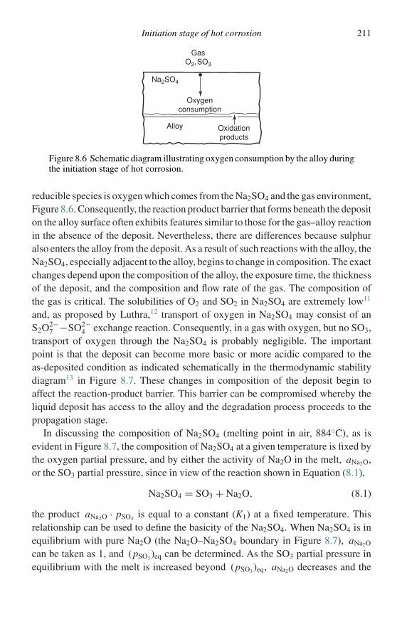
Initiation stage of hot corrosion 211
GasO2,SO3
Na2SO4
Oxygenconsumption
Alloy Oxidationproducts
Figure 8.6 Schematic diagram illustrating oxygen consumption by the alloy duringthe initiation stage of hot corrosion.
reducible species is oxygen which comes from the Na2SO4 and the gas environment,Figure 8.6. Consequently, the reaction product barrier that forms beneath the depositon the alloy surface often exhibits features similar to those for the gas–alloy reactionin the absence of the deposit. Nevertheless, there are differences because sulphuralso enters the alloy from the deposit. As a result of such reactions with the alloy, theNa2SO4, especially adjacent to the alloy, begins to change in composition. The exactchanges depend upon the composition of the alloy, the exposure time, the thicknessof the deposit, and the composition and flow rate of the gas. The composition ofthe gas is critical. The solubilities of O2 and SO2 in Na2SO4 are extremely low11
and, as proposed by Luthra,12 transport of oxygen in Na2SO4 may consist of anS2O2−
7 −SO2−4 exchange reaction. Consequently, in a gas with oxygen, but no SO3,
transport of oxygen through the Na2SO4 is probably negligible. The importantpoint is that the deposit can become more basic or more acidic compared to theas-deposited condition as indicated schematically in the thermodynamic stabilitydiagram13 in Figure 8.7. These changes in composition of the deposit begin toaffect the reaction-product barrier. This barrier can be compromised whereby theliquid deposit has access to the alloy and the degradation process proceeds to thepropagation stage.
In discussing the composition of Na2SO4 (melting point in air, 884◦C), as isevident in Figure 8.7, the composition of Na2SO4 at a given temperature is fixed bythe oxygen partial pressure, and by either the activity of Na2O in the melt, aNa2O,or the SO3 partial pressure, since in view of the reaction shown in Equation (8.1),
Na2SO4 = SO3 + Na2O, (8.1)
the product aNa2O · pSO3 is equal to a constant (K1) at a fixed temperature. Thisrelationship can be used to define the basicity of the Na2SO4. When Na2SO4 is inequilibrium with pure Na2O (the Na2O–Na2SO4 boundary in Figure 8.7), aNa2O
can be taken as 1, and (pSO3)eq can be determined. As the SO3 partial pressure inequilibrium with the melt is increased beyond (pSO3)eq, aNa2O decreases and the
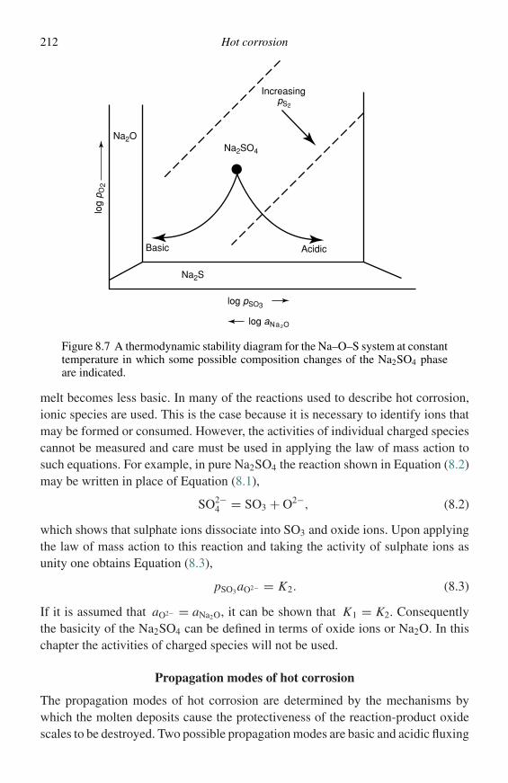
212 Hot corrosion
Na2ONa2SO4
Na2S
log
p O2
log pSO3
log aNa2O
pS2
Increasing
Basic Acidic
Figure 8.7 A thermodynamic stability diagram for the Na–O–S system at constanttemperature in which some possible composition changes of the Na2SO4 phaseare indicated.
melt becomes less basic. In many of the reactions used to describe hot corrosion,ionic species are used. This is the case because it is necessary to identify ions thatmay be formed or consumed. However, the activities of individual charged speciescannot be measured and care must be used in applying the law of mass action tosuch equations. For example, in pure Na2SO4 the reaction shown in Equation (8.2)may be written in place of Equation (8.1),
SO2−4 = SO3 + O2−, (8.2)
which shows that sulphate ions dissociate into SO3 and oxide ions. Upon applyingthe law of mass action to this reaction and taking the activity of sulphate ions asunity one obtains Equation (8.3),
pSO3aO2− = K2. (8.3)
If it is assumed that aO2− = aNa2O, it can be shown that K1 = K2. Consequentlythe basicity of the Na2SO4 can be defined in terms of oxide ions or Na2O. In thischapter the activities of charged species will not be used.
Propagation modes of hot corrosion
The propagation modes of hot corrosion are determined by the mechanisms bywhich the molten deposits cause the protectiveness of the reaction-product oxidescales to be destroyed. Two possible propagation modes are basic and acidic fluxing
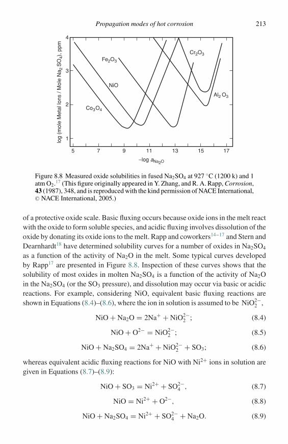
Propagation modes of hot corrosion 213
Fe2O3
Co3O4
NiO
Cr2O3
Al2 O3
5 7 9 11 13 15 17
−log aNa2O
4
3
2
1log
(mol
e M
etal
lons
/ M
ole
Na 2
SO
4), p
pm
Figure 8.8 Measured oxide solubilities in fused Na2SO4 at 927 ◦C (1200 k) and 1atm O2.17 (This figure originally appeared in Y. Zhang, and R. A. Rapp, Corrosion,43 (1987), 348, and is reproduced with the kind permission of NACE International,C© NACE International, 2005.)
of a protective oxide scale. Basic fluxing occurs because oxide ions in the melt reactwith the oxide to form soluble species, and acidic fluxing involves dissolution of theoxide by donating its oxide ions to the melt. Rapp and coworkers14–17 and Stern andDearnhardt18 have determined solubility curves for a number of oxides in Na2SO4
as a function of the activity of Na2O in the melt. Some typical curves developedby Rapp17 are presented in Figure 8.8. Inspection of these curves shows that thesolubility of most oxides in molten Na2SO4 is a function of the activity of Na2Oin the Na2SO4 (or the SO3 pressure), and dissolution may occur via basic or acidicreactions. For example, considering NiO, equivalent basic fluxing reactions areshown in Equations (8.4)–(8.6), where the ion in solution is assumed to be NiO2−
2 ,
NiO + Na2O = 2Na+ + NiO2−2 ; (8.4)
NiO + O2− = NiO2−2 ; (8.5)
NiO + Na2SO4 = 2Na+ + NiO2−2 + SO3; (8.6)
whereas equivalent acidic fluxing reactions for NiO with Ni2+ ions in solution aregiven in Equations (8.7)–(8.9):
NiO + SO3 = Ni2+ + SO2−4 , (8.7)
NiO = Ni2+ + O2−, (8.8)
NiO + Na2SO4 = Ni2+ + SO2−4 + Na2O. (8.9)
214 Hot corrosion
The NiO dissolves by either accepting oxide ions (basic) or by donating oxide ions(acidic). There is a minimum in the solubility curve at the point where the basic andacidic dissolution curves intersect and the slopes of these curves are determined byEquations (8.4)–(8.6) with slope = 1 and by Equations (8.7)–(8.9) with slope = −1,respectively. If, during the dissolution process, the metal ion changes valence, forexample, Ni2+ → Ni3+, then the dissolution reaction will be dependent upon theoxygen partial pressure. For example, for the reaction shown in Equation (8.10),
2NiO + Na2O + 1
2O2 = 2Na+ + 2NiO−
2 , (8.10)
the slope of the dissolution curve, Figure 8.8, will be 1/2 (for a constant oxygenpressure) rather than 1 as it is for NiO2−
2 ions.In discussing fluxing processes the variation of solubilities of oxides as a function
of thickness across the salt is crucial. Rapp and Goto19 have proposed for continuedhot corrosion of a pure metal that the gradient in the solubility of the protective oxide(COxide) in the salt film is negative at the oxide–salt interface, Equation (8.11),(
dCOxide
dx
)x=0
< 0, (8.11)
where x is the thickness of the deposit. This condition allows the oxide to dissolveat the oxide–salt ( x = 0) interface and precipitate out in the salt as discontinuousparticles ( x > 0). When this solubility gradient is positive the salt becomes sat-urated with oxide and protective oxide will eventually form at the metal surface.Shores20 has examined the Rapp–Goto criterion for fluxing and has shown that forsome cases this criterion cannot be sustained indefinitely as a function of expo-sure time. Nevertheless, as will be shown subsequently, even when transitory, thiscriterion is an important aspect of hot corrosion processes. In fact the transitorycondition may be close to practice because in many cases, especially gas turbines,deposits are formed intermittently. Shores20 has also considered the form of the saltdeposit on the metal surface and has shown that in many cases the salt distributesitself in pores of the oxide scale. Surface tension effects play a significant role indetermining the distribution of the salt. It is reasonable to consider the salt depositas a continuous layer on the surface of the metal or alloy during the initiation stageof hot corrosion, but as the propagation stage becomes dominant the salt is morelikely to be distributed in the pores of the non-protective oxide and consequentlythe attack may not be uniform over all of the specimen’s surface.
There are other propagation modes in addition to the fluxing propagation modes.For example, as will be shown in more detail subsequently, in the case of Na2SO4-induced hot corrosion a significant amount of sulphur can be transferred from theNa2SO4 into the metal or alloy. In some alloys the oxidation of these sulphides isa major factor in the degradation. Hence, oxidation of sulphides is a propagation
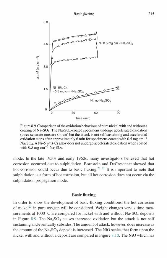
Basic fluxing 215
Ni, no Na2SO4
Ni, 0.5 mg cm−2 Na2SO4
Ni–5% Cr, −0.5 mg cm−2Na2SO4
Time (min)
00
30 60 90
1.5
3.0
4.5
6.0
∆m
/A (
mg
cm−2
)
Figure 8.9 Comparison of the oxidation behaviour of pure nickel with and without acoating of Na2SO4. The Na2SO4-coated specimens undergo accelerated oxidation(three separate runs are shown) but the attack is not self sustaining and acceleratedoxidation stops after approximately 6 min for specimens coated with 0.5 mg cm−2
Na2SO4. A Ni–5 wt% Cr alloy does not undergo accelerated oxidation when coatedwith 0.5 mg cm−2 Na2SO4.
mode. In the late 1950s and early 1960s, many investigators believed that hotcorrosion occurred due to sulphidation. Bornstein and DeCrescente showed thathot corrosion could occur due to basic fluxing.21,22 It is important to note thatsulphidation is a form of hot corrosion, but all hot corrosion does not occur via thesulphidation propagation mode.
Basic fluxing
In order to show the development of basic-fluxing conditions, the hot corrosionof nickel23 in pure oxygen will be considered. Weight changes versus time mea-surements at 1000 ◦C are compared for nickel with and without Na2SO4 depositsin Figure 8.9. The Na2SO4 causes increased oxidation but the attack is not selfsustaining and eventually subsides. The amount of attack, however, does increase asthe amount of the Na2SO4 deposit is increased. The NiO scales that form upon thenickel with and without a deposit are compared in Figure 8.10. The NiO which has
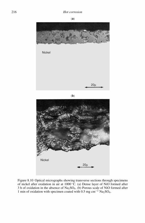
216 Hot corrosion
Nickel
Nickel
(b)
(a)
Ni0
Ni0
20µ
20µ
Figure 8.10 Optical micrographs showing transverse sections through specimensof nickel after oxidation in air at 1000 ◦C. (a) Dense layer of NiO formed after3 h of oxidation in the absence of Na2SO4. (b) Porous scale of NiO formed after1 min of oxidation with specimen coated with 0.5 mg cm−2 Na2SO4.
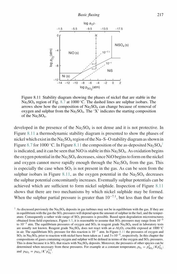
Basic fluxing 217
log aO2−
log pSO3(atm)
log
p O2(a
tm)
NiO (s)
Ni (s)
NiS
NiSO4 (s)
−14
−1.5 −5.5 −9.5 −13.5 −17.5
−12 −10 −8 −6 −4 −2
0
−4
−8
−120 2
10−7.1
10−1
Figure 8.11 Stability diagram showing the phases of nickel that are stable in theNa2SO4 region of Fig. 8.7 at 1000 ◦C. The dashed lines are sulphur isobars. Thearrows show how the composition of Na2SO4 can change because of removal ofoxygen and sulphur from the Na2SO4. The ‘X’ indicates the starting compositionof the Na2SO4.
developed in the presence of the Na2SO4 is not dense and it is not protective. InFigure 8.11 a thermodynamic stability diagram is presented to show the phases ofnickel which exist in the Na2SO4 region of the Na–S–O stability diagram as shown inFigure 8.7 for 1000 ◦C. In Figure 8.11 the composition of the as-deposited Na2SO4
†
is indicated, and it can be seen that NiO is stable in this Na2SO4. As oxidation beginsthe oxygen potential in the Na2SO4 decreases, since NiO begins to form on the nickeland oxygen cannot move rapidly enough through the Na2SO4 from the gas. Thisis especially the case when SO3 is not present in the gas. As can be seen from thesulphur isobars in Figure 8.11, as the oxygen potential in the Na2SO4 decreasesthe sulphur potential concomitantly increases. Eventually sulphur potentials can beachieved which are sufficient to form nickel sulphide. Inspection of Figure 8.11shows that there are two mechanisms by which nickel sulphide may be formed.When the sulphur partial pressure is greater than 10−7.1, but less than that for the
† As discussed previously the Na2SO4 deposits in gas turbines may not be in equilibrium with the gas. If they arein equilibrium with the gas the SO3 pressures will depend upon the amount of sulphur in the fuel, and the temper-ature. Consequently a rather wide range of SO3 pressures is possible. Based upon degradation microstructuresobtained from field experience, Figure 8.5, it is reasonable to assume that SO3 pressures may range from 10−5
to 10−3 atm. The equilibrium pressures of oxygen and SO3 in reagent grade Na2SO4 used in laboratory testsare usually not known. Reagent grade Na2SO4 does not react with an α-Al2O3 crucible exposed at 1000 ◦Cin air. The equilibrium SO3 pressure for this reaction is 10−7 atm. In Figure 8.11 the pressures of oxygen andSO3 in Na2SO4 prior to reaction with nickel have been taken as 1 and 3×10⁻⁵, respectively. In this chapter thecompositions of gases containing oxygen and sulphur will be defined in terms of the oxygen and SO3 pressures.This is done because it is SO3 that reacts with Na2SO4 deposits. Moreover, the pressures of other species can bedetermined when necessary from these pressures. For example at a constant temperature, pS2 = p2
SO3/K p3
O2;
and pSO2 = pSO3 /K ′ p1/2O2
.
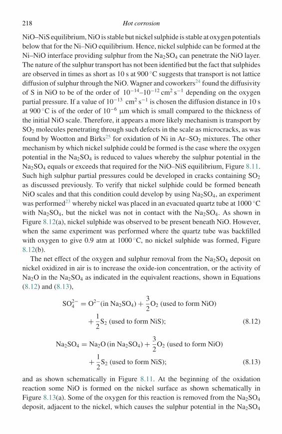
218 Hot corrosion
NiO–NiS equilibrium, NiO is stable but nickel sulphide is stable at oxygen potentialsbelow that for the Ni–NiO equilibrium. Hence, nickel sulphide can be formed at theNi–NiO interface providing sulphur from the Na2SO4 can penetrate the NiO layer.The nature of the sulphur transport has not been identified but the fact that sulphidesare observed in times as short as 10 s at 900 ◦C suggests that transport is not latticediffusion of sulphur through the NiO. Wagner and coworkers24 found the diffusivityof S in NiO to be of the order of 10−14–10−12 cm2 s−1 depending on the oxygenpartial pressure. If a value of 10−13 cm2 s−1 is chosen the diffusion distance in 10 sat 900 ◦C is of the order of 10−6 µm which is small compared to the thickness ofthe initial NiO scale. Therefore, it appears a more likely mechanism is transport bySO2 molecules penetrating through such defects in the scale as microcracks, as wasfound by Wootton and Birks25 for oxidation of Ni in Ar–SO2 mixtures. The othermechanism by which nickel sulphide could be formed is the case where the oxygenpotential in the Na2SO4 is reduced to values whereby the sulphur potential in theNa2SO4 equals or exceeds that required for the NiO–NiS equilibrium, Figure 8.11.Such high sulphur partial pressures could be developed in cracks containing SO2
as discussed previously. To verify that nickel sulphide could be formed beneathNiO scales and that this condition could develop by using Na2SO4, an experimentwas performed23 whereby nickel was placed in an evacuated quartz tube at 1000 ◦Cwith Na2SO4, but the nickel was not in contact with the Na2SO4. As shown inFigure 8.12(a), nickel sulphide was observed to be present beneath NiO. However,when the same experiment was performed where the quartz tube was backfilledwith oxygen to give 0.9 atm at 1000 ◦C, no nickel sulphide was formed, Figure8.12(b).
The net effect of the oxygen and sulphur removal from the Na2SO4 deposit onnickel oxidized in air is to increase the oxide-ion concentration, or the activity ofNa2O in the Na2SO4 as indicated in the equivalent reactions, shown in Equations(8.12) and (8.13),
SO2−4 = O2−(in Na2SO4) + 3
2O2 (used to form NiO)
+ 1
2S2 (used to form NiS); (8.12)
Na2SO4 = Na2O (in Na2SO4) + 3
2O2 (used to form NiO)
+ 1
2S2 (used to form NiS); (8.13)
and as shown schematically in Figure 8.11. At the beginning of the oxidationreaction some NiO is formed on the nickel surface as shown schematically inFigure 8.13(a). Some of the oxygen for this reaction is removed from the Na2SO4
deposit, adjacent to the nickel, which causes the sulphur potential in the Na2SO4
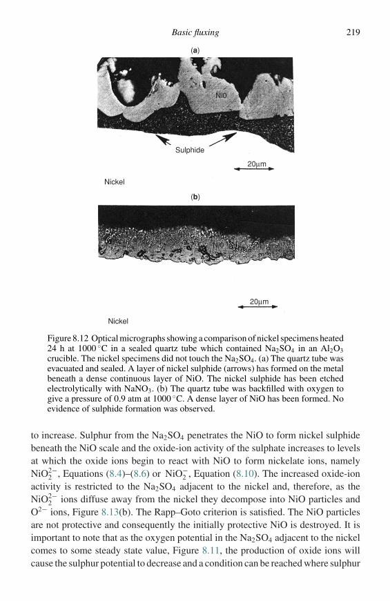
Basic fluxing 219
(b)
(a)
Sulphide
Nickel
Nickel
20µm
20µm
Ni0
Ni0
Figure 8.12 Optical micrographs showing a comparison of nickel specimens heated24 h at 1000 ◦C in a sealed quartz tube which contained Na2SO4 in an Al2O3crucible. The nickel specimens did not touch the Na2SO4. (a) The quartz tube wasevacuated and sealed. A layer of nickel sulphide (arrows) has formed on the metalbeneath a dense continuous layer of NiO. The nickel sulphide has been etchedelectrolytically with NaNO3. (b) The quartz tube was backfilled with oxygen togive a pressure of 0.9 atm at 1000 ◦C. A dense layer of NiO has been formed. Noevidence of sulphide formation was observed.
to increase. Sulphur from the Na2SO4 penetrates the NiO to form nickel sulphidebeneath the NiO scale and the oxide-ion activity of the sulphate increases to levelsat which the oxide ions begin to react with NiO to form nickelate ions, namelyNiO2−
2 , Equations (8.4)–(8.6) or NiO−2 , Equation (8.10). The increased oxide-ion
activity is restricted to the Na2SO4 adjacent to the nickel and, therefore, as theNiO2−
2 ions diffuse away from the nickel they decompose into NiO particles andO2− ions, Figure 8.13(b). The Rapp–Goto criterion is satisfied. The NiO particlesare not protective and consequently the initially protective NiO is destroyed. It isimportant to note that as the oxygen potential in the Na2SO4 adjacent to the nickelcomes to some steady state value, Figure 8.11, the production of oxide ions willcause the sulphur potential to decrease and a condition can be reached where sulphur
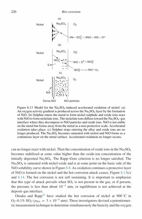
220 Hot corrosion
Nickel
Nickel
Nickel
NiS
NiO particlesDense NiO
Na2SO4
Na2SO4
Na2SO4
(b)
(c)
(a)
4Ni + SO42− = 3NiO + NiS + O2−
NiO + O2−= NiO22−
NiO22−
O2
O2
O2
NiO22−−
S
NiO + O2−
Figure 8.13 Model for the Na2SO4-induced accelerated oxidation of nickel. (a)An oxygen activity gradient is produced across the Na2SO4 layer by the formationof NiO. (b) Sulphur enters the metal to form nickel sulphide and oxide ions reactwith NiO to form nickelate ions. The nickelate ions diffuse toward the Na2SO4–gasinterface where they decompose to NiO particles and oxide ions. NiO is not stableon the metal but forms away from the metal as a non-protective scale. Acceleratedoxidation takes place. (c) Sulphur stops entering the alloy and oxide ions are nolonger produced. The Na2SO4 becomes saturated with nickel and NiO forms as acontinuous layer on the metal surface. Accelerated oxidation no longer occurs.
can no longer react with nickel. Then the concentration of oxide ions in the Na2SO4
becomes stabilized at some value higher than the oxide-ion concentration of theinitially deposited Na2SO4. The Rapp–Goto criterion is no longer satisfied. TheNa2SO4 is saturated with nickel oxide and is at some point on the basic side of theNiO solubility curve shown in Figure 8.8. As oxidation continues a protective layerof NiO is formed on the nickel and the hot corrosion attack ceases, Figure 8.13(c)and 8.14. The hot corrosion is not self sustaining. It is important to emphasizethat this type of attack prevails when SO3 is not present in the gas, or if present,the pressure is less than about 10−3 atm, or equilibrium is not achieved at thedeposit–gas interface.
Otsuka and Rapp26 have studied the hot corrosion of nickel at 900 ◦C inO2–0.1% SO2 (pSO3 = 3 × 10⁻⁴ atm). These investigators devised a potentiomet-ric measurement technique to determine simultaneously the basicity and the oxygen
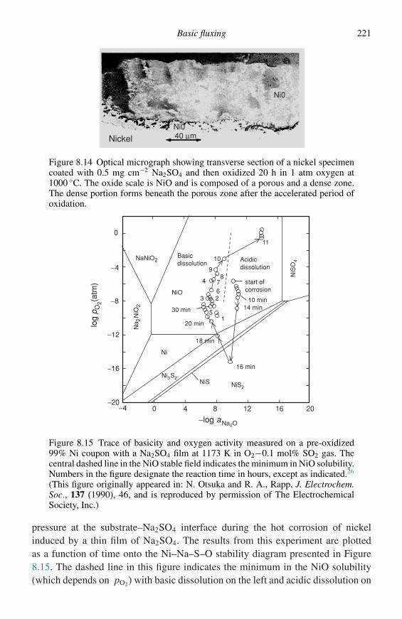
Basic fluxing 221
Nickel 40 µm
Ni0
Ni0
Figure 8.14 Optical micrograph showing transverse section of a nickel specimencoated with 0.5 mg cm−2 Na2SO4 and then oxidized 20 h in 1 atm oxygen at1000 ◦C. The oxide scale is NiO and is composed of a porous and a dense zone.The dense portion forms beneath the porous zone after the accelerated period ofoxidation.
−log aNa2O
log
p O2(a
tm)
Basicdissolution
Acidicdissolution
30 min
20 min
18 min
16 min
14 min10 min
NiO
Ni
NiS NiS2
Ni3S2
NaNiO2
Na 2
NiO
2
NiS
O4
start ofcorrosion
11
10
98
76
5
4
3 2
1
201612840−4−20
−16
−12
−8
−4
0
Figure 8.15 Trace of basicity and oxygen activity measured on a pre-oxidized99% Ni coupon with a Na2SO4 film at 1173 K in O2−0.1 mol% SO2 gas. Thecentral dashed line in the NiO stable field indicates the minimum in NiO solubility.Numbers in the figure designate the reaction time in hours, except as indicated.26
(This figure originally appeared in: N. Otsuka and R. A., Rapp, J. Electrochem.Soc., 137 (1990), 46, and is reproduced by permission of The ElectrochemicalSociety, Inc.)
pressure at the substrate–Na2SO4 interface during the hot corrosion of nickelinduced by a thin film of Na2SO4. The results from this experiment are plottedas a function of time onto the Ni–Na–S–O stability diagram presented in Figure8.15. The dashed line in this figure indicates the minimum in the NiO solubility(which depends on pO2) with basic dissolution on the left and acidic dissolution on
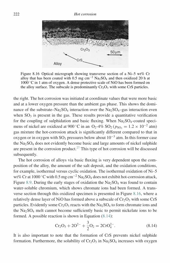
222 Hot corrosion
50µm
Alloy
Cr2O3
CrS
Ni0
Figure 8.16 Optical micrograph showing transverse section of a Ni–5 wt% Cralloy that has been coated with 0.5 mg cm−2 Na2SO4 and then oxidized 20 h at1000 ◦C in 1 atm of oxygen. A dense protective scale of NiO has been formed onthe alloy surface. The subscale is predominantly Cr2O3 with some CrS particles.
the right. The hot corrosion was initiated at coordinate values that were more basicand at a lower oxygen pressure than the ambient gas phase. This shows the domi-nance of the substrate–Na2SO4 interaction over the Na2SO4–gas interaction evenwhen SO3 is present in the gas. These results provide a quantitative verificationfor the coupling of sulphidation and basic fluxing. When Na2SO4-coated speci-mens of nickel are oxidized at 900 ◦C in an O2-4% SO2 (pSO3 = 1.2 × 10⁻² atm)gas mixture the hot-corrosion attack is significantly different compared to that inoxygen or in oxygen with SO3 pressures below about 10−3 atm. In this former casethe Na2SO4 does not evidently become basic and large amounts of nickel sulphideare present in the corrosion product.27 This type of hot corrosion will be discussedsubsequently.
The hot corrosion of alloys via basic fluxing is very dependent upon the com-position of the alloy, the amount of the salt deposit, and the oxidation conditions,for example, isothermal versus cyclic oxidation. The isothermal oxidation of Ni–5wt% Cr at 1000 ◦C with 0.5 mg cm−2 Na2SO4 does not exhibit hot-corrosion attack,Figure 8.9. During the early stages of oxidation the Na2SO4 was found to containwater-soluble chromium, which shows chromate ions had been formed. A trans-verse section through this oxidized specimen is presented in Figure 8.16, where arelatively dense layer of NiO has formed above a subscale of Cr2O3 with some CrSparticles. Evidently some Cr2O3 reacts with the Na2SO4 to form chromate ions andthe Na2SO4 melt cannot become sufficiently basic to permit nickelate ions to beformed. A possible reaction is shown in Equation (8.14):
Cr2O3 + 2O2− + 3
2O2 = 2CrO2−
4 . (8.14)
It is also important to note that the formation of CrS prevents nickel sulphideformation. Furthermore, the solubility of Cr2O3 in Na2SO4 increases with oxygen
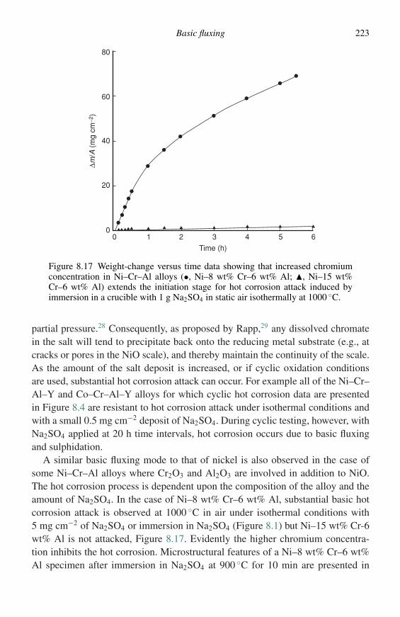
Basic fluxing 223
Time (h)
∆m/A
(m
g cm
−2)
80
60
40
20
00 1 2 3 4 5 6
Figure 8.17 Weight-change versus time data showing that increased chromiumconcentration in Ni–Cr–Al alloys (•, Ni–8 wt% Cr–6 wt% Al; �, Ni–15 wt%Cr–6 wt% Al) extends the initiation stage for hot corrosion attack induced byimmersion in a crucible with 1 g Na2SO4 in static air isothermally at 1000 ◦C.
partial pressure.28 Consequently, as proposed by Rapp,29 any dissolved chromatein the salt will tend to precipitate back onto the reducing metal substrate (e.g., atcracks or pores in the NiO scale), and thereby maintain the continuity of the scale.As the amount of the salt deposit is increased, or if cyclic oxidation conditionsare used, substantial hot corrosion attack can occur. For example all of the Ni–Cr–Al–Y and Co–Cr–Al–Y alloys for which cyclic hot corrosion data are presentedin Figure 8.4 are resistant to hot corrosion attack under isothermal conditions andwith a small 0.5 mg cm−2 deposit of Na2SO4. During cyclic testing, however, withNa2SO4 applied at 20 h time intervals, hot corrosion occurs due to basic fluxingand sulphidation.
A similar basic fluxing mode to that of nickel is also observed in the case ofsome Ni–Cr–Al alloys where Cr2O3 and Al2O3 are involved in addition to NiO.The hot corrosion process is dependent upon the composition of the alloy and theamount of Na2SO4. In the case of Ni–8 wt% Cr–6 wt% Al, substantial basic hotcorrosion attack is observed at 1000 ◦C in air under isothermal conditions with5 mg cm−2 of Na2SO4 or immersion in Na2SO4 (Figure 8.1) but Ni–15 wt% Cr-6wt% Al is not attacked, Figure 8.17. Evidently the higher chromium concentra-tion inhibits the hot corrosion. Microstructural features of a Ni–8 wt% Cr–6 wt%Al specimen after immersion in Na2SO4 at 900 ◦C for 10 min are presented in
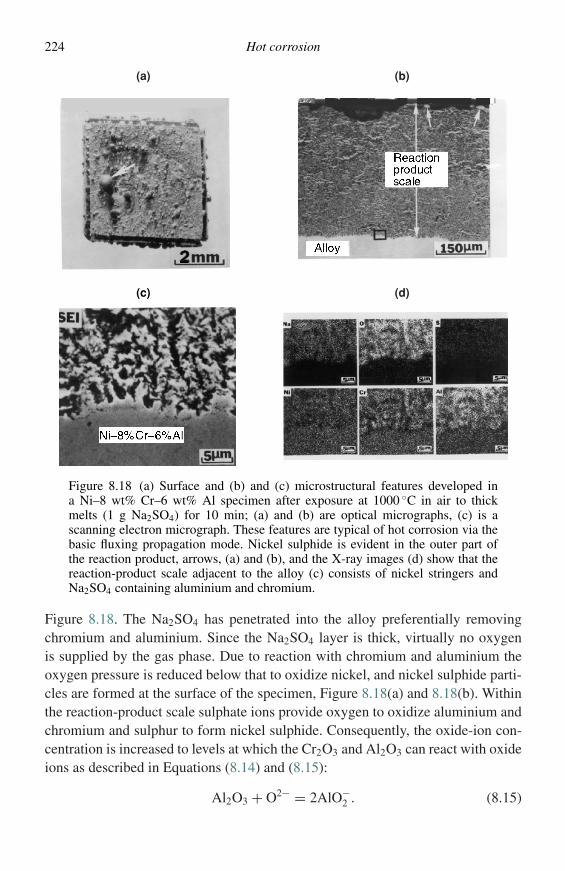
224 Hot corrosion
(a) (b)
(c) (d)
Figure 8.18 (a) Surface and (b) and (c) microstructural features developed ina Ni–8 wt% Cr–6 wt% Al specimen after exposure at 1000 ◦C in air to thickmelts (1 g Na2SO4) for 10 min; (a) and (b) are optical micrographs, (c) is ascanning electron micrograph. These features are typical of hot corrosion via thebasic fluxing propagation mode. Nickel sulphide is evident in the outer part ofthe reaction product, arrows, (a) and (b), and the X-ray images (d) show that thereaction-product scale adjacent to the alloy (c) consists of nickel stringers andNa2SO4 containing aluminium and chromium.
Figure 8.18. The Na2SO4 has penetrated into the alloy preferentially removingchromium and aluminium. Since the Na2SO4 layer is thick, virtually no oxygenis supplied by the gas phase. Due to reaction with chromium and aluminium theoxygen pressure is reduced below that to oxidize nickel, and nickel sulphide parti-cles are formed at the surface of the specimen, Figure 8.18(a) and 8.18(b). Withinthe reaction-product scale sulphate ions provide oxygen to oxidize aluminium andchromium and sulphur to form nickel sulphide. Consequently, the oxide-ion con-centration is increased to levels at which the Cr2O3 and Al2O3 can react with oxideions as described in Equations (8.14) and (8.15):
Al2O3 + O2− = 2AlO−2 . (8.15)
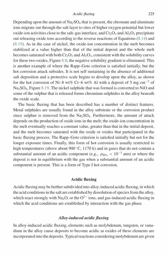
Acidic fluxing 225
Depending upon the amount of Na2SO4 that is present, the chromate and aluminateions migrate out through the salt layer to sites of higher oxygen potential but loweroxide-ion activities close to the salt–gas interface, and Cr2O3 and Al2O3 precipitateout releasing oxide ions according to the reverse reactions of Equations (8.14) and(8.15). As in the case of nickel, the oxide-ion concentration in the melt becomesstabilized at a value higher than that of the initial deposit and the whole meltbecomes saturated with both Cr2O3 and Al2O3, consistent with the solubility curvesfor these two oxides, Figure 8.8; the negative solubility gradient is eliminated. Thisis another example of where the Rapp–Goto criterion is satisfied initially, but thehot corrosion attack subsides. It is not self sustaining in the absence of additionalsalt deposition and a protective scale begins to develop upon the alloy, as shownfor the hot corrosion of Ni–8 wt% Cr–6 wt% Al with a deposit of 5 mg cm−2 ofNa2SO4, Figure 8.19. The nickel sulphide that was formed is converted to NiO andsome of the sulphur that is released forms chromium sulphides in the alloy beneaththe oxide scale.
The basic fluxing that has been described has a number of distinct features.Metal sulphides are usually found in the alloy substrate or the corrosion productsince sulphur is removed from the Na2SO4. Furthermore, the amount of attackdepends on the production of oxide ions in the melt; the oxide-ion concentration inthe melt eventually reaches a constant value, greater than that in the initial deposit,and the melt becomes saturated with the oxide or oxides that participated in thebasic fluxing process. The Rapp–Goto criterion is satisfied initially but not for thelonger exposure times. Finally, this form of hot corrosion is usually restricted tohigh temperatures (above about 900 ◦C, 1170 k) and in gases that do not contain asubstantial amount of an acidic component (e.g., pSO3 < 10−3 atm) or where thedeposit is not in equilibrium with the gas when a substantial amount of an acidiccomponent is present. This is a form of Type I hot corrosion.
Acidic fluxing
Acidic fluxing may be further subdivided into alloy-induced acidic fluxing, in whichthe acid conditions in the salt are established by dissolution of species from the alloy,which react strongly with Na2O, or the O2− ions, and gas-induced acidic fluxing inwhich the acid conditions are established by interaction with the gas phase.
Alloy-induced acidic fluxing
In alloy-induced acidic fluxing, elements such as molybdenum, tungsten, or vana-dium in the alloy cause deposits to become acidic as oxides of these elements areincorporated into the deposits. Typical reactions considering molybdenum are given
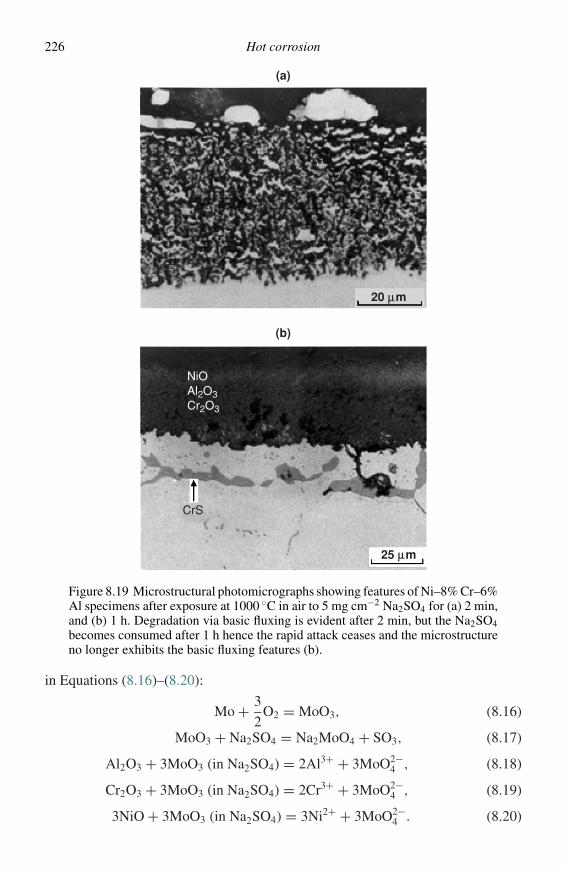
226 Hot corrosion
25 µm
20 µm
(b)
CrS
NiOAl2O3Cr2O3
(a)
Figure 8.19 Microstructural photomicrographs showing features of Ni–8% Cr–6%Al specimens after exposure at 1000 ◦C in air to 5 mg cm−2 Na2SO4 for (a) 2 min,and (b) 1 h. Degradation via basic fluxing is evident after 2 min, but the Na2SO4becomes consumed after 1 h hence the rapid attack ceases and the microstructureno longer exhibits the basic fluxing features (b).
in Equations (8.16)–(8.20):
Mo + 3
2O2 = MoO3, (8.16)
MoO3 + Na2SO4 = Na2MoO4 + SO3, (8.17)
Al2O3 + 3MoO3 (in Na2SO4) = 2Al3+ + 3MoO2−4 , (8.18)
Cr2O3 + 3MoO3 (in Na2SO4) = 2Cr3+ + 3MoO2−4 , (8.19)
3NiO + 3MoO3 (in Na2SO4) = 3Ni2+ + 3MoO2−4 . (8.20)
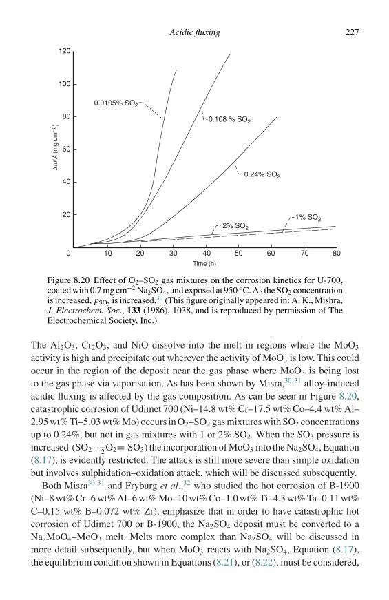
Acidic fluxing 227
0.0105% SO2
0.108 % SO2
0.24% SO2
1% SO22% SO2
Time (h)
∆m/A
(m
g cm
−2)
120
100
80
60
40
20
0 10 20 30 40 50 60 70 80
Figure 8.20 Effect of O2–SO2 gas mixtures on the corrosion kinetics for U-700,coated with 0.7 mg cm−2 Na2SO4, and exposed at 950 ◦C. As the SO2 concentrationis increased, pSO3 is increased.30 (This figure originally appeared in: A. K., Mishra,J. Electrochem. Soc., 133 (1986), 1038, and is reproduced by permission of TheElectrochemical Society, Inc.)
The Al2O3, Cr2O3, and NiO dissolve into the melt in regions where the MoO3
activity is high and precipitate out wherever the activity of MoO3 is low. This couldoccur in the region of the deposit near the gas phase where MoO3 is being lostto the gas phase via vaporisation. As has been shown by Misra,30,31 alloy-inducedacidic fluxing is affected by the gas composition. As can be seen in Figure 8.20,catastrophic corrosion of Udimet 700 (Ni–14.8 wt% Cr–17.5 wt% Co–4.4 wt% Al–2.95 wt% Ti–5.03 wt% Mo) occurs in O2–SO2 gas mixtures with SO2 concentrationsup to 0.24%, but not in gas mixtures with 1 or 2% SO2. When the SO3 pressure isincreased (SO2+ 1
2 O2= SO3) the incorporation of MoO3 into the Na2SO4, Equation(8.17), is evidently restricted. The attack is still more severe than simple oxidationbut involves sulphidation–oxidation attack, which will be discussed subsequently.
Both Misra30,31 and Fryburg et al.,32 who studied the hot corrosion of B-1900(Ni–8 wt% Cr–6 wt% Al–6 wt% Mo–10 wt% Co–1.0 wt% Ti–4.3 wt% Ta–0.11 wt%C–0.15 wt% B–0.072 wt% Zr), emphasize that in order to have catastrophic hotcorrosion of Udimet 700 or B-1900, the Na2SO4 deposit must be converted to aNa2MoO4–MoO3 melt. Melts more complex than Na2SO4 will be discussed inmore detail subsequently, but when MoO3 reacts with Na2SO4, Equation (8.17),the equilibrium condition shown in Equations (8.21), or (8.22), must be considered,
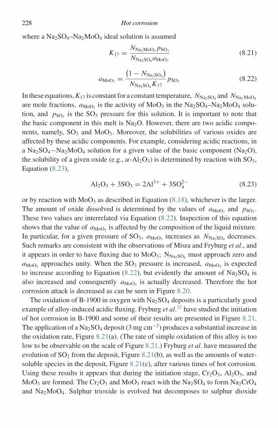
228 Hot corrosion
where a Na2SO4–Na2MoO4 ideal solution is assumed
K17 = NNa2MoO4 pSO3
NNa2SO4aMoO3
(8.21)
aMoO3 =(1 − NNa2SO4
)NNa2SO4 K17
pSO3 (8.22)
In these equations, K17 is constant for a constant temperature, NNa2SO4 and NNa2 MoO4
are mole fractions, aMoO3 is the activity of MoO3 in the Na2SO4–Na2MoO4 solu-tion, and pSO3 is the SO3 pressure for this solution. It is important to note thatthe basic component in this melt is Na2O. However, there are two acidic compo-nents, namely, SO3 and MoO3. Moreover, the solubilities of various oxides areaffected by these acidic components. For example, considering acidic reactions, ina Na2SO4−Na2MoO4 solution for a given value of the basic component (Na2O),the solubility of a given oxide (e.g., α-Al2O3) is determined by reaction with SO3,Equation (8.23),
Al2O3 + 3SO3 = 2Al3+ + 3SO2−4 (8.23)
or by reaction with MoO3 as described in Equation (8.18), whichever is the larger.The amount of oxide dissolved is determined by the values of aMoO3 and pSO3 .These two values are interrelated via Equation (8.22). Inspection of this equationshows that the value of aMoO3 is affected by the composition of the liquid mixture.In particular, for a given pressure of SO3, aMoO3 increases as NNa2SO4 decreases.Such remarks are consistent with the observations of Misra and Fryburg et al., andit appears in order to have fluxing due to MoO3; NNa2SO4 must approach zero andaMoO3 approaches unity. When the SO3 pressure is increased, aMoO3 is expectedto increase according to Equation (8.22), but evidently the amount of Na2SO4 isalso increased and consequently aMoO3 is actually decreased. Therefore the hotcorrosion attack is decreased as can be seen in Figure 8.20.
The oxidation of B-1900 in oxygen with Na2SO4 deposits is a particularly goodexample of alloy-induced acidic fluxing. Fryburg et al.32 have studied the initiationof hot corrosion in B-1900 and some of their results are presented in Figure 8.21.The application of a Na2SO4 deposit (3 mg cm−2) produces a substantial increase inthe oxidation rate, Figure 8.21(a). (The rate of simple oxidation of this alloy is toolow to be observable on the scale of Figure 8.21.) Fryburg et al. have measured theevolution of SO2 from the deposit, Figure 8.21(b), as well as the amounts of water-soluble species in the deposit, Figure 8.21(c), after various times of hot corrosion.Using these results it appears that during the initiation stage, Cr2O3, Al2O3, andMoO3 are formed. The Cr2O3 and MoO3 react with the Na2SO4 to form Na2CrO4
and Na2MoO4. Sulphur trioxide is evolved but decomposes to sulphur dioxide
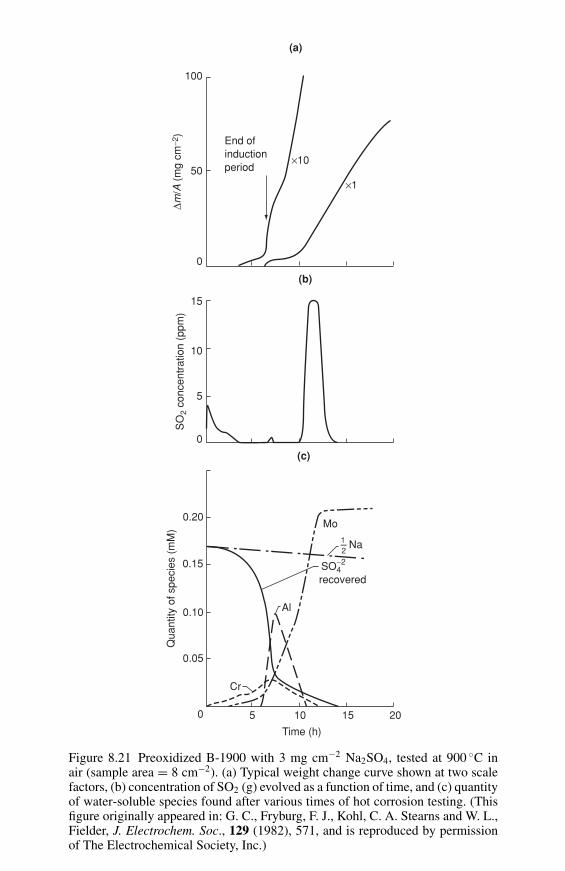
(a)
(b)
(c)
Qua
ntity
of s
peci
es (
mM
)S
O2
conc
entr
atio
n (p
pm)
∆m/A
(m
g cm
−2)
recovered
1–2 Na
End ofinductionperiod
×10
×1
100
50
0
15
10
5
0
5 10 15 20
Time (h)
Mo
SO4−2
Al
Cr
0
0.20
0.15
0.10
0.05
Figure 8.21 Preoxidized B-1900 with 3 mg cm−2 Na2SO4, tested at 900 ◦C inair (sample area = 8 cm−2). (a) Typical weight change curve shown at two scalefactors, (b) concentration of SO2 (g) evolved as a function of time, and (c) quantityof water-soluble species found after various times of hot corrosion testing. (Thisfigure originally appeared in: G. C., Fryburg, F. J., Kohl, C. A. Stearns and W. L.,Fielder, J. Electrochem. Soc., 129 (1982), 571, and is reproduced by permissionof The Electrochemical Society, Inc.)
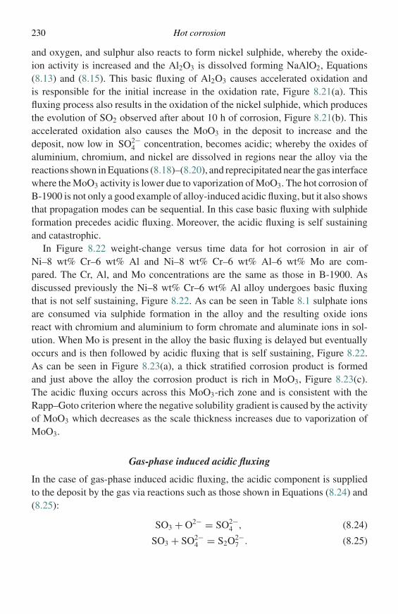
230 Hot corrosion
and oxygen, and sulphur also reacts to form nickel sulphide, whereby the oxide-ion activity is increased and the Al2O3 is dissolved forming NaAlO2, Equations(8.13) and (8.15). This basic fluxing of Al2O3 causes accelerated oxidation andis responsible for the initial increase in the oxidation rate, Figure 8.21(a). Thisfluxing process also results in the oxidation of the nickel sulphide, which producesthe evolution of SO2 observed after about 10 h of corrosion, Figure 8.21(b). Thisaccelerated oxidation also causes the MoO3 in the deposit to increase and thedeposit, now low in SO2−
4 concentration, becomes acidic; whereby the oxides ofaluminium, chromium, and nickel are dissolved in regions near the alloy via thereactions shown in Equations (8.18)–(8.20), and reprecipitated near the gas interfacewhere the MoO3 activity is lower due to vaporization of MoO3. The hot corrosion ofB-1900 is not only a good example of alloy-induced acidic fluxing, but it also showsthat propagation modes can be sequential. In this case basic fluxing with sulphideformation precedes acidic fluxing. Moreover, the acidic fluxing is self sustainingand catastrophic.
In Figure 8.22 weight-change versus time data for hot corrosion in air ofNi–8 wt% Cr–6 wt% Al and Ni–8 wt% Cr–6 wt% Al–6 wt% Mo are com-pared. The Cr, Al, and Mo concentrations are the same as those in B-1900. Asdiscussed previously the Ni–8 wt% Cr–6 wt% Al alloy undergoes basic fluxingthat is not self sustaining, Figure 8.22. As can be seen in Table 8.1 sulphate ionsare consumed via sulphide formation in the alloy and the resulting oxide ionsreact with chromium and aluminium to form chromate and aluminate ions in sol-ution. When Mo is present in the alloy the basic fluxing is delayed but eventuallyoccurs and is then followed by acidic fluxing that is self sustaining, Figure 8.22.As can be seen in Figure 8.23(a), a thick stratified corrosion product is formedand just above the alloy the corrosion product is rich in MoO3, Figure 8.23(c).The acidic fluxing occurs across this MoO3-rich zone and is consistent with theRapp–Goto criterion where the negative solubility gradient is caused by the activityof MoO3 which decreases as the scale thickness increases due to vaporization ofMoO3.
Gas-phase induced acidic fluxing
In the case of gas-phase induced acidic fluxing, the acidic component is suppliedto the deposit by the gas via reactions such as those shown in Equations (8.24) and(8.25):
SO3 + O2− = SO2−4 , (8.24)
SO3 + SO2−4 = S2O2−
7 . (8.25)
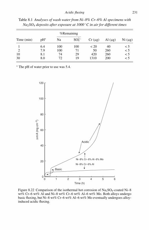
Acidic fluxing 231
Table 8.1 Analyses of wash water from Ni–8% Cr–6% Al specimens withNa2SO4 deposits after exposure at 1000 ◦C in air for different times
%Remaining
Time (min) pH∗ Na SO42− Cr (µg) Al (µg) Ni (µg)
1 6.4 100 100 < 20 40 < 52 7.9 100 71 50 260 < 5
10 8.1 74 29 420 260 < 530 8.0 72 19 1310 200 < 5
∗ The pH of water prior to use was 5.4.
120
100
80
60
40
20
00 1 2 3 4 5 6
∆m/A
(m
g cm
−2)
Acidic
Basic
Ni−8% Cr−6% Al−6% Mo
Ni−8% Cr−6% Al
Time (h)
Figure 8.22 Comparison of the isothermal hot corrosion of Na2SO4-coated Ni–8wt% Cr–6 wt% Al and Ni–8 wt% Cr–6 wt% Al–6 wt% Mo. Both alloys undergobasic fluxing, but Ni–8 wt% Cr–6 wt% Al–6 wt% Mo eventually undergoes alloy-induced acidic fluxing.
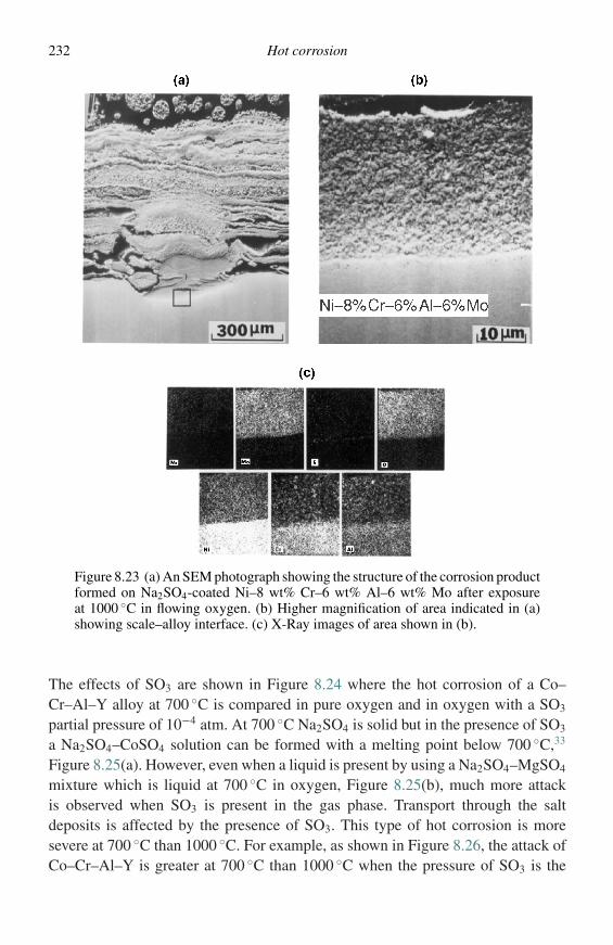
232 Hot corrosion
Figure 8.23 (a) An SEM photograph showing the structure of the corrosion productformed on Na2SO4-coated Ni–8 wt% Cr–6 wt% Al–6 wt% Mo after exposureat 1000 ◦C in flowing oxygen. (b) Higher magnification of area indicated in (a)showing scale–alloy interface. (c) X-Ray images of area shown in (b).
The effects of SO3 are shown in Figure 8.24 where the hot corrosion of a Co–Cr–Al–Y alloy at 700 ◦C is compared in pure oxygen and in oxygen with a SO3
partial pressure of 10−4 atm. At 700 ◦C Na2SO4 is solid but in the presence of SO3
a Na2SO4–CoSO4 solution can be formed with a melting point below 700 ◦C,33
Figure 8.25(a). However, even when a liquid is present by using a Na2SO4–MgSO4
mixture which is liquid at 700 ◦C in oxygen, Figure 8.25(b), much more attackis observed when SO3 is present in the gas phase. Transport through the saltdeposits is affected by the presence of SO3. This type of hot corrosion is moresevere at 700 ◦C than 1000 ◦C. For example, as shown in Figure 8.26, the attack ofCo–Cr–Al–Y is greater at 700 ◦C than 1000 ◦C when the pressure of SO3 is the
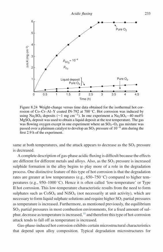
Acidic fluxing 233
∆m/A
(m
g cm
−2)
Time (h)
Pure O2
Pure O2
Pure O2
pO2
pSO3
= 10−4
Liquid deposit
6
5
4
3
2
1
0 0.5 1.5 2.5 3.5 4.51 2 3 4
}
Figure 8.24 Weight-change versus time data obtained for the isothermal hot cor-rosion of Co–Cr–Al–Y coated IN-792 at 700 ◦C. Hot corrosion was induced byusing Na2SO4 deposits (∼1 mg cm−2). In one experiment a Na2SO4−40 mol%MgSO4 deposit was used to obtain a liquid deposit at the test temperature. The gaswas flowing oxygen except in one experiment where an SO2–O2 gas mixture waspassed over a platinum catalyst to develop an SO3 pressure of 10−4 atm during thefirst 2.9 h of the experiment.
same at both temperatures, and the attack appears to decrease as the SO3 pressureis decreased.
A complete description of gas-phase acidic fluxing is difficult because the effectsare different for different metals and alloys. Also, as the SO3 pressure is increasedsulphide formation in the alloy begins to play more of a role in the degradationprocess. One distinctive feature of this type of hot corrosion is that the degradationrates are greater at low temperatures (e.g., 650–750 ◦C) compared to higher tem-peratures (e.g., 950–1000 ◦C). Hence it is often called ‘low-temperature’ or TypeII hot corrosion. This low-temperature characteristic results from the need to formsulphates such as CoSO4 and NiSO4 (not necessarily at unit activity), which arenecessary to form liquid sulphate solutions and require higher SO3 partial pressuresas temperature is increased. Furthermore, as mentioned previously, the equilibriumSO3 partial pressures in most combustion environments, for a fixed amount of sul-phur, decrease as temperature is increased,10 and therefore this type of hot-corrosionattack tends to fall off as temperature is increased.
Gas-phase-induced hot corrosion exhibits certain microstructural characteristicsthat depend upon alloy composition. Typical degradation microstructures for
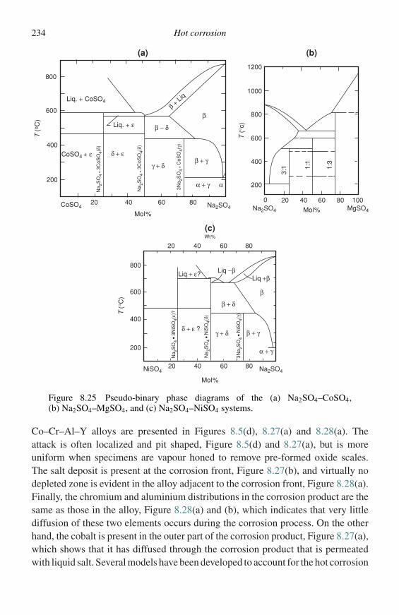
234 Hot corrosion
(c)
T (
°C)
20
800
600
400
200
20 40 60 80
40 60 80
NiSO4 Na2SO4
Mol%
Na 2
SO
4 •
3NiS
O4(
ε)?
Na
2SO
4 •
NiS
O4(
δ)
3Na 2
SO
4 •
NiS
O4(
γ)
α + γ
β + γ γ + δ
β + δ
δ + ε ?
β
Liq +βLiq −βLiq + ε?
Wt%
(b)
T (
°c)
1200
1000
800
600
400
200
0 20 40 60 80 100Na2SO4 MgSO4Mol%
3:1 1:
1
1:3
(a)
T (
o C)
800
600
400
200
20 40 60 80CoSO4
CoSO4 + ε
Liq. + CoSO4
Liq. + ε
β + Liq
Na2SO4
Na
2SO
4 . 3
CoS
O4(
δ)
3Na 2
SO
4 . C
oSO
4(γ)
Na 2
SO
4 . 3
CoS
O4(
δ)
β + γγ + δ
δ + ε
β − δ
α + γ
Mol%
β
α
Figure 8.25 Pseudo-binary phase diagrams of the (a) Na2SO4–CoSO4,(b) Na2SO4–MgSO4, and (c) Na2SO4–NiSO4 systems.
Co–Cr–Al–Y alloys are presented in Figures 8.5(d), 8.27(a) and 8.28(a). Theattack is often localized and pit shaped, Figure 8.5(d) and 8.27(a), but is moreuniform when specimens are vapour honed to remove pre-formed oxide scales.The salt deposit is present at the corrosion front, Figure 8.27(b), and virtually nodepleted zone is evident in the alloy adjacent to the corrosion front, Figure 8.28(a).Finally, the chromium and aluminium distributions in the corrosion product are thesame as those in the alloy, Figure 8.28(a) and (b), which indicates that very littlediffusion of these two elements occurs during the corrosion process. On the otherhand, the cobalt is present in the outer part of the corrosion product, Figure 8.27(a),which shows that it has diffused through the corrosion product that is permeatedwith liquid salt. Several models have been developed to account for the hot corrosion
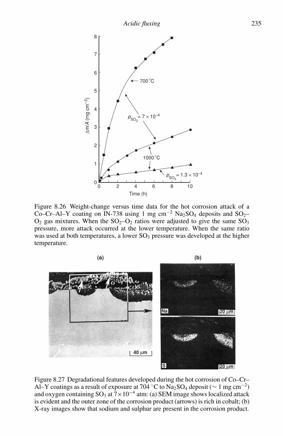
Acidic fluxing 235
Time (h)
∆m/A
(m
g cm
−2)
pSO3
= 7 × 10⁻⁴
pSO3
= 1.3 × 10⁻⁴
700°C
1000°C
8
7
6
5
4
3
2
1
00 2 4 6 8 10
Figure 8.26 Weight-change versus time data for the hot corrosion attack of aCo–Cr–Al–Y coating on IN-738 using 1 mg cm−2 Na2SO4 deposits and SO2–O2 gas mixtures. When the SO2–O2 ratios were adjusted to give the same SO3pressure, more attack occurred at the lower temperature. When the same ratiowas used at both temperatures, a lower SO3 pressure was developed at the highertemperature.
(a) (b)
40 µm
20 µm
20 µmNa
S
Figure 8.27 Degradational features developed during the hot corrosion of Co–Cr–Al–Y coatings as a result of exposure at 704 ◦C to Na2SO4 deposit (∼ 1 mg cm−2)and oxygen containing SO3 at 7×10⁻⁴ atm: (a) SEM image shows localized attackis evident and the outer zone of the corrosion product (arrows) is rich in cobalt; (b)X-ray images show that sodium and sulphur are present in the corrosion product.
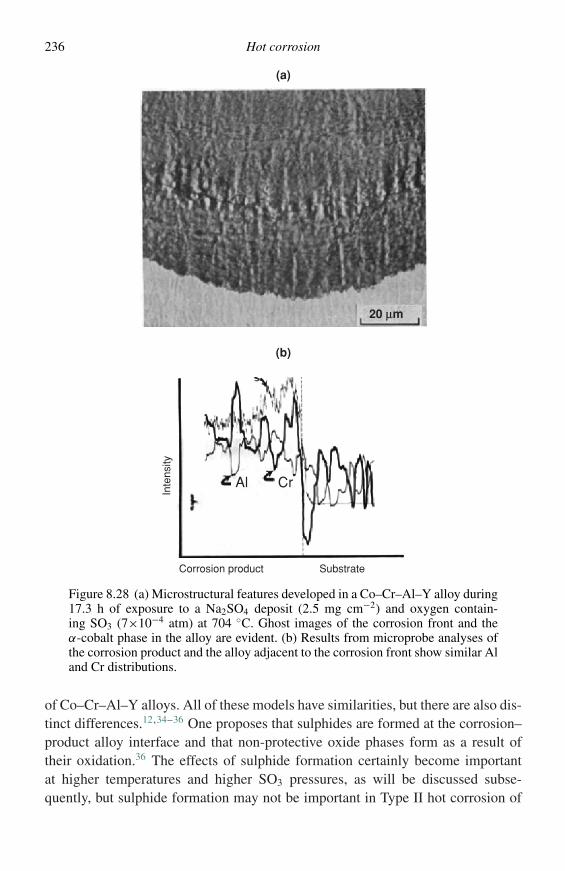
236 Hot corrosion
Al Cr
(b)
(a)
Corrosion product Substrate
Inte
nsity
20 µm
Figure 8.28 (a) Microstructural features developed in a Co–Cr–Al–Y alloy during17.3 h of exposure to a Na2SO4 deposit (2.5 mg cm−2) and oxygen contain-ing SO3 (7×10⁻⁴ atm) at 704 ◦C. Ghost images of the corrosion front and theα-cobalt phase in the alloy are evident. (b) Results from microprobe analyses ofthe corrosion product and the alloy adjacent to the corrosion front show similar Aland Cr distributions.
of Co–Cr–Al–Y alloys. All of these models have similarities, but there are also dis-tinct differences.12,34–36 One proposes that sulphides are formed at the corrosion–product alloy interface and that non-protective oxide phases form as a result oftheir oxidation.36 The effects of sulphide formation certainly become importantat higher temperatures and higher SO3 pressures, as will be discussed subse-quently, but sulphide formation may not be important in Type II hot corrosion of
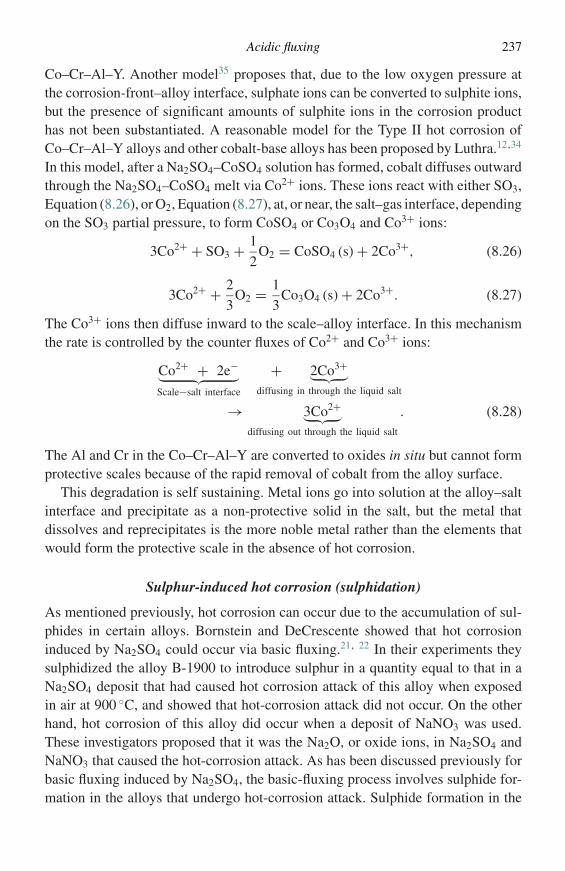
Acidic fluxing 237
Co–Cr–Al–Y. Another model35 proposes that, due to the low oxygen pressure atthe corrosion-front–alloy interface, sulphate ions can be converted to sulphite ions,but the presence of significant amounts of sulphite ions in the corrosion producthas not been substantiated. A reasonable model for the Type II hot corrosion ofCo–Cr–Al–Y alloys and other cobalt-base alloys has been proposed by Luthra.12,34
In this model, after a Na2SO4–CoSO4 solution has formed, cobalt diffuses outwardthrough the Na2SO4–CoSO4 melt via Co2+ ions. These ions react with either SO3,Equation (8.26), or O2, Equation (8.27), at, or near, the salt–gas interface, dependingon the SO3 partial pressure, to form CoSO4 or Co3O4 and Co3+ ions:
3Co2+ + SO3 + 1
2O2 = CoSO4 (s) + 2Co3+, (8.26)
3Co2+ + 2
3O2 = 1
3Co3O4 (s) + 2Co3+. (8.27)
The Co3+ ions then diffuse inward to the scale–alloy interface. In this mechanismthe rate is controlled by the counter fluxes of Co2+ and Co3+ ions:
Co2+ + 2e−︸ ︷︷ ︸Scale−salt interface
+ 2Co3+︸ ︷︷ ︸diffusing in through the liquid salt
→ 3Co2+︸ ︷︷ ︸diffusing out through the liquid salt
. (8.28)
The Al and Cr in the Co–Cr–Al–Y are converted to oxides in situ but cannot formprotective scales because of the rapid removal of cobalt from the alloy surface.
This degradation is self sustaining. Metal ions go into solution at the alloy–saltinterface and precipitate as a non-protective solid in the salt, but the metal thatdissolves and reprecipitates is the more noble metal rather than the elements thatwould form the protective scale in the absence of hot corrosion.
Sulphur-induced hot corrosion (sulphidation)
As mentioned previously, hot corrosion can occur due to the accumulation of sul-phides in certain alloys. Bornstein and DeCrescente showed that hot corrosioninduced by Na2SO4 could occur via basic fluxing.21, 22 In their experiments theysulphidized the alloy B-1900 to introduce sulphur in a quantity equal to that in aNa2SO4 deposit that had caused hot corrosion attack of this alloy when exposedin air at 900 ◦C, and showed that hot-corrosion attack did not occur. On the otherhand, hot corrosion of this alloy did occur when a deposit of NaNO3 was used.These investigators proposed that it was the Na2O, or oxide ions, in Na2SO4 andNaNO3 that caused the hot-corrosion attack. As has been discussed previously forbasic fluxing induced by Na2SO4, the basic-fluxing process involves sulphide for-mation in the alloys that undergo hot-corrosion attack. Sulphide formation in the
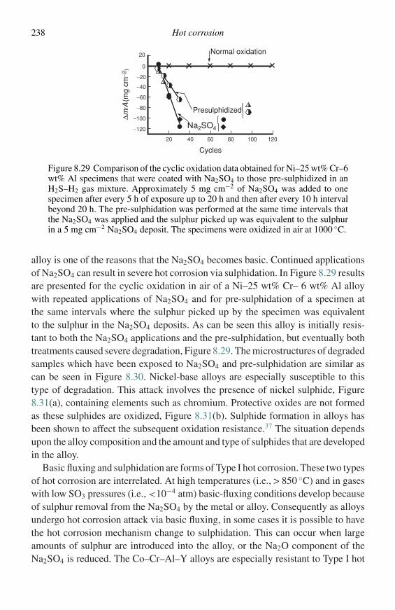
238 Hot corrosion
12010080604020
−120
−100
−80
−60
−40
−20
0
20
Na2SO4
Presulphidized
Cycles
Normal oxidation
∆m/A
(mg
cm−2
)
Figure 8.29 Comparison of the cyclic oxidation data obtained for Ni–25 wt% Cr–6wt% Al specimens that were coated with Na2SO4 to those pre-sulphidized in anH2S–H2 gas mixture. Approximately 5 mg cm−2 of Na2SO4 was added to onespecimen after every 5 h of exposure up to 20 h and then after every 10 h intervalbeyond 20 h. The pre-sulphidation was performed at the same time intervals thatthe Na2SO4 was applied and the sulphur picked up was equivalent to the sulphurin a 5 mg cm−2 Na2SO4 deposit. The specimens were oxidized in air at 1000 ◦C.
alloy is one of the reasons that the Na2SO4 becomes basic. Continued applicationsof Na2SO4 can result in severe hot corrosion via sulphidation. In Figure 8.29 resultsare presented for the cyclic oxidation in air of a Ni–25 wt% Cr– 6 wt% Al alloywith repeated applications of Na2SO4 and for pre-sulphidation of a specimen atthe same intervals where the sulphur picked up by the specimen was equivalentto the sulphur in the Na2SO4 deposits. As can be seen this alloy is initially resis-tant to both the Na2SO4 applications and the pre-sulphidation, but eventually bothtreatments caused severe degradation, Figure 8.29. The microstructures of degradedsamples which have been exposed to Na2SO4 and pre-sulphidation are similar ascan be seen in Figure 8.30. Nickel-base alloys are especially susceptible to thistype of degradation. This attack involves the presence of nickel sulphide, Figure8.31(a), containing elements such as chromium. Protective oxides are not formedas these sulphides are oxidized, Figure 8.31(b). Sulphide formation in alloys hasbeen shown to affect the subsequent oxidation resistance.37 The situation dependsupon the alloy composition and the amount and type of sulphides that are developedin the alloy.
Basic fluxing and sulphidation are forms of Type I hot corrosion. These two typesof hot corrosion are interrelated. At high temperatures (i.e., > 850 ◦C) and in gaseswith low SO3 pressures (i.e., <10−4 atm) basic-fluxing conditions develop becauseof sulphur removal from the Na2SO4 by the metal or alloy. Consequently as alloysundergo hot corrosion attack via basic fluxing, in some cases it is possible to havethe hot corrosion mechanism change to sulphidation. This can occur when largeamounts of sulphur are introduced into the alloy, or the Na2O component of theNa2SO4 is reduced. The Co–Cr–Al–Y alloys are especially resistant to Type I hot
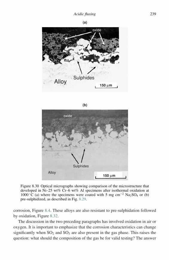
Acidic fluxing 239
Alloy
Alloy
Sulphides
Sulphides
oxide
oxide
(a)
(b)
150 µm
150 µm
Figure 8.30 Optical micrographs showing comparison of the microstructure thatdeveloped in Ni–25 wt% Cr–6 wt% Al specimens after isothermal oxidation at1000 ◦C (a) where the specimens were coated with 5 mg cm−2 Na2SO4 or (b)pre-sulphidized, as described in Fig. 8.29.
corrosion, Figure 8.4. These alloys are also resistant to pre-sulphidation followedby oxidation, Figure 8.32.
The discussion in the two preceding paragraphs has involved oxidation in air oroxygen. It is important to emphasize that the corrosion characteristics can changesignificantly when SO2 and SO3 are also present in the gas phase. This raises thequestion: what should the composition of the gas be for valid testing? The answer
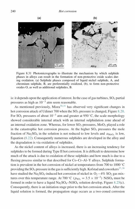
240 Hot corrosion
(a) (b)
Figure 8.31 Photomicrographs to illustrate the mechanism by which sulphidephases in alloys can result in the formation of non-protective oxide scales dur-ing oxidation. (a) Sulphide phases composed of liquid nickel sulphide, A, andchromium sulphide, B, are preferentially oxidized, (b), to form non-protectiveoxides O, as well as additional sulphides, B.
is: it depends upon the application of interest. In the case of gas turbines, SO3 partialpressures as high as 10−3 atm seem reasonable.
As mentioned previously, Misra30,31 has observed very significant changes inhot corrosion attack of Udimet 700 when the SO3 pressure is changed, Figure 8.20.For SO3 pressures of about 10−3 atm and greater at 950 ◦C, the scale morphologyshowed considerable internal attack with an internal sulphidation zone ahead ofan internal oxidation zone. Whereas, for lower SO3 pressures, MoO3 played a rolein the catastrophic hot corrosion process. At the higher SO3 pressures the molefraction of Na2SO4 in the solution is not reduced to low levels and aMoO3 is low,Equation (8.22). Consequently numerous sulphides are developed in the alloy andthe degradation is via oxidation of sulphides.
As the nickel content of alloys is increased, there is an increasing tendency forsulphides to be formed during Type II hot corrosion. It is difficult to determine howmuch of the attack is due to oxidation of these sulphides and how much is due to afluxing process similar to that described for Co–Cr–Al–Y alloys. Sulphide forma-tion is prevalent in the hot corrosion of nickel at temperatures from 700 to 1000 ◦Cproviding the SO3 pressure in the gas is sufficiently high. Kofstad and coworkers27,38
have studied the Na2SO4-induced hot corrosion of nickel in O2−4% SO2 gas mix-tures over this temperature range. At 700 ◦C (pSO3 = 3.5 × 10⁻²) NiSO4 must beformed in order to have a liquid Na2SO4–NiSO4 solution develop, Figure 8.25(c).Consequently, there is an initiation stage prior to the hot corrosion attack. After theliquid solution is formed, the propagation stage occurs as a two-zoned corrosion
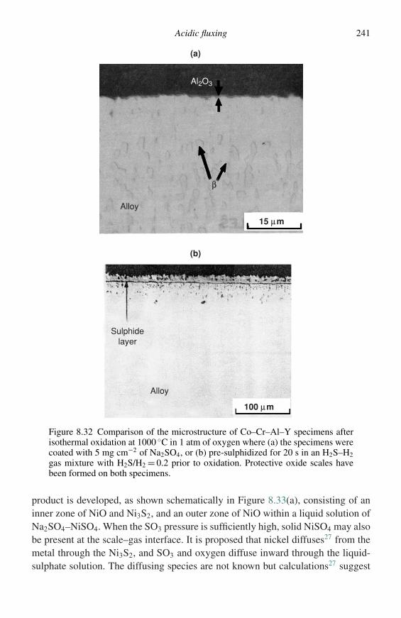
Acidic fluxing 241
15 µm
100 µm
Alloy
Alloy
Al2O3
(b)
(a)
β
Sulphidelayer
Figure 8.32 Comparison of the microstructure of Co–Cr–Al–Y specimens afterisothermal oxidation at 1000 ◦C in 1 atm of oxygen where (a) the specimens werecoated with 5 mg cm−2 of Na2SO4, or (b) pre-sulphidized for 20 s in an H2S–H2gas mixture with H2S/H2 = 0.2 prior to oxidation. Protective oxide scales havebeen formed on both specimens.
product is developed, as shown schematically in Figure 8.33(a), consisting of aninner zone of NiO and Ni3S2, and an outer zone of NiO within a liquid solution ofNa2SO4–NiSO4. When the SO3 pressure is sufficiently high, solid NiSO4 may alsobe present at the scale–gas interface. It is proposed that nickel diffuses27 from themetal through the Ni3S2, and SO3 and oxygen diffuse inward through the liquid-sulphate solution. The diffusing species are not known but calculations27 suggest
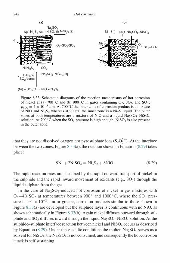
242 Hot corrosion
NiO
Ni/Ni3S2
NiONi3S2
S/Ni3S2
NiSO4 (s) Ni–S(l) NiO–NiSO4 (l)Na2SO4
Na2SO4−NiSO4
(Na2SO4−NiSO4)liq
Ni
SO3
(Ni) + SO3/O NiO + Ni3S2
SO2/pores
Ni O2+SO2 /SO3
SO3
(a) (b)
O2+SO2/SO3
Figure 8.33 Schematic diagrams of the reaction mechanisms of hot corrosionof nickel at (a) 700 ◦C and (b) 900 ◦C in gases containing O2, SO2, and SO3;pSO3 = 4 × 10⁻³ atm. At 700 ◦C the inner zone of corrosion product is a mixtureof NiO and Ni3S2 whereas at 900 ◦C the inner zone is a Ni–S liquid. The outerzones at both temperatures are a mixture of NiO and a liquid Na2SO4–NiSO4solution. At 700 ◦C when the SO3 pressure is high enough, NiSO4 is also presentin the outer zone.
that they are not dissolved oxygen nor pyrosulphate ions (S2O2−7 ). At the interface
between the two zones, Figure 8.33(a), the reaction shown in Equation (8.29) takesplace:
9Ni + 2NiSO4 = Ni3S2 + 8NiO. (8.29)
The rapid reaction rates are sustained by the rapid outward transport of nickel inthe sulphide and the rapid inward movement of oxidants (e.g., SO3) through theliquid sulphate from the gas.
In the case of Na2SO4-induced hot corrosion of nickel in gas mixtures withO2−4% SO2 at temperatures between 900 ◦ and 1000 ◦C, where the SO3 pres-sure is ∼1 × 10⁻² atm or greater, corrosion products similar to those shown inFigure 8.33(a) are developed but the sulphide layer is continuous with no NiO, asshown schematically in Figure 8.33(b). Again nickel diffuses outward through sul-phide and SO3 diffuses inward through the liquid Na2SO4–NiSO4 solution. At thesulphide–sulphate interface reaction between nickel and NiSO4 occurs as describedby Equation (8.29). Under these acidic conditions the molten Na2SO4 serves as asolvent for NiSO4, the Na2SO4 is not consumed, and consequently the hot corrosionattack is self sustaining.
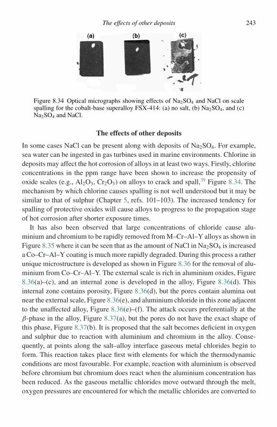
The effects of other deposits 243
Figure 8.34 Optical micrographs showing effects of Na2SO4 and NaCl on scalespalling for the cobalt-base superalloy FSX-414: (a) no salt, (b) Na2SO4, and (c)Na2SO4 and NaCl.
The effects of other deposits
In some cases NaCl can be present along with deposits of Na2SO4. For example,sea water can be ingested in gas turbines used in marine environments. Chlorine indeposits may affect the hot corrosion of alloys in at least two ways. Firstly, chlorineconcentrations in the ppm range have been shown to increase the propensity ofoxide scales (e.g., Al2O3, Cr2O3) on alloys to crack and spall,39 Figure 8.34. Themechanism by which chlorine causes spalling is not well understood but it may besimilar to that of sulphur (Chapter 5, refs. 101–103). The increased tendency forspalling of protective oxides will cause alloys to progress to the propagation stageof hot corrosion after shorter exposure times.
It has also been observed that large concentrations of chloride cause alu-minium and chromium to be rapidly removed from M–Cr–Al–Y alloys as shown inFigure 8.35 where it can be seen that as the amount of NaCl in Na2SO4 is increaseda Co–Cr–Al–Y coating is much more rapidly degraded. During this process a ratherunique microstructure is developed as shown in Figure 8.36 for the removal of alu-minium from Co–Cr–Al–Y. The external scale is rich in aluminium oxides, Figure8.36(a)–(c), and an internal zone is developed in the alloy, Figure 8.36(d). Thisinternal zone contains porosity, Figure 8.36(d), but the pores contain alumina outnear the external scale, Figure 8.36(e), and aluminium chloride in this zone adjacentto the unaffected alloy, Figure 8.36(e)–(f). The attack occurs preferentially at theβ-phase in the alloy, Figure 8.37(a), but the pores do not have the exact shape ofthis phase, Figure 8.37(b). It is proposed that the salt becomes deficient in oxygenand sulphur due to reaction with aluminium and chromium in the alloy. Conse-quently, at points along the salt–alloy interface gaseous metal chlorides begin toform. This reaction takes place first with elements for which the thermodynamicconditions are most favourable. For example, reaction with aluminium is observedbefore chromium but chromium does react when the aluminium concentration hasbeen reduced. As the gaseous metallic chlorides move outward through the melt,oxygen pressures are encountered for which the metallic chlorides are converted to
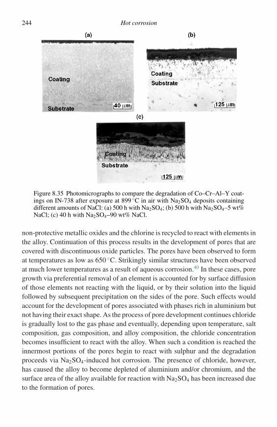
244 Hot corrosion
Figure 8.35 Photomicrographs to compare the degradation of Co–Cr–Al–Y coat-ings on IN-738 after exposure at 899 ◦C in air with Na2SO4 deposits containingdifferent amounts of NaCl: (a) 500 h with Na2SO4; (b) 500 h with Na2SO4–5 wt%NaCl; (c) 40 h with Na2SO4–90 wt% NaCl.
non-protective metallic oxides and the chlorine is recycled to react with elements inthe alloy. Continuation of this process results in the development of pores that arecovered with discontinuous oxide particles. The pores have been observed to format temperatures as low as 650 ◦C. Strikingly similar structures have been observedat much lower temperatures as a result of aqueous corrosion.40 In these cases, poregrowth via preferential removal of an element is accounted for by surface diffusionof those elements not reacting with the liquid, or by their solution into the liquidfollowed by subsequent precipitation on the sides of the pore. Such effects wouldaccount for the development of pores associated with phases rich in aluminium butnot having their exact shape. As the process of pore development continues chlorideis gradually lost to the gas phase and eventually, depending upon temperature, saltcomposition, gas composition, and alloy composition, the chloride concentrationbecomes insufficient to react with the alloy. When such a condition is reached theinnermost portions of the pores begin to react with sulphur and the degradationproceeds via Na2SO4-induced hot corrosion. The presence of chloride, however,has caused the alloy to become depleted of aluminium and/or chromium, and thesurface area of the alloy available for reaction with Na2SO4 has been increased dueto the formation of pores.
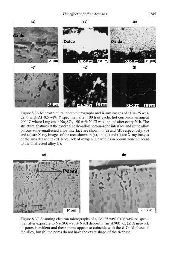
The effects of other deposits 245
Figure 8.36 Microstructural photomicrographs and X-ray images of a Co–25 wt%Cr–6 wt% Al–0.5 wt% Y specimen after 100 h of cyclic hot corrosion testing at900 ◦C where 1 mg cm−2 Na2SO4−90 wt% NaCl was applied after every 20 h. Thestructural features at the external scale–alloy porous-zone interface and at the alloyporous-zone–unaffected alloy interface are shown in (a) and (d), respectively; (b)and (c) are X-ray images of the area shown in (a), and (e) and (f) are X-ray imagesof the area defined in (d). Note lack of oxygen in particles in porous zone adjacentto the unaffected alloy (f).
Figure 8.37 Scanning electron micrographs of a Co–25 wt% Cr–6 wt% Al speci-men after exposure to Na2SO4−90% NaCl deposit in air at 900 ◦C. (a) A networkof pores is evident and these pores appear to coincide with the β-CoAl phase ofthe alloy, but (b) the pores do not have the exact shape of the β-phase.
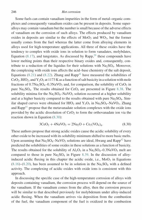
246 Hot corrosion
Some fuels can contain vanadium impurities in the form of metal–organic com-plexes and consequently vanadium oxides can be present in deposits. Some super-alloys may contain vanadium but the number is small because of the adverse effectsof vanadium on the corrosion of such alloys. The effects produced by vanadiumoxides in deposits are similar to the effects of MoO3 and WO3, but the formerusually comes from the fuel whereas the latter come from alloying elements inalloys used for high-temperature applications. All three of these oxides have thetendency to complex with oxide ions in solution to form vanadates, molybdates,Equation (8.17), and tungstates. As discussed by Rapp,29 these compounds havelower melting points than their respective binary oxides and, consequently, con-tribute to a reduction of the liquidus for their solutions with Na2SO4. Moreover,the complexing with oxide ions affects the acid–base chemistry of the salt deposit,Equations (8.21) and (8.22). Zhang and Rapp41 have measured the solubilities ofCeO2, HfO2, and Y2O3 at 1173 K as a function of salt basicity in a solution with molefractions of 0.7Na2SO4–0.3NaVO3 and, for comparison, the solubility of CeO2 inpure Na2SO4. The results obtained for CeO2 are presented in Figure 8.38. Thesolubility minima for the Na2SO4–NaVO3 solution occurred at a higher solubilityand at a higher basicity compared to the results obtained with pure Na2SO4. Sim-ilar shaped curves were obtained for HfO2 and Y2O3 in Na2SO4–NaVO3. Zhangand Rapp41 propose that the metavanadate solution complexes with the oxide ionsprovided by the acidic dissolution of CeO2 to form the orthovanadate ion via thereaction shown in Equation (8.30):
3CeO2 + 4NaVO3 = 2Na2O + Ce3(VO4)4. (8.30)
These authors propose that strong acidic oxides cause the acidic solubility of everyother oxide to be increased with its solubility minimum shifted to more basic melts.Upon assuming that Na2SO4–NaVO3 solutions are ideal, Hwang and Rapp42 havepredicted the solubilities of some oxides in these solutions as a function of basicity.The results obtained for the solubility of Al2O3 in a Na2SO4–0.3NaVO3 melt arecompared to those in pure Na2SO4 in Figure 8.39. In the discussion of alloy-induced acidic fluxing in this chapter the acidic oxide, i.e., MoO3 in Equations(8.16)–(8.20), has been assumed to be in solution in the Na2SO4 with a definedactivity. The complexing of acidic oxides with oxide ions is consistent with thisapproach.
In discussing the specific case of the high-temperature corrosion of alloys withdeposits containing vanadium, the corrosion process will depend on the source ofthe vanadium. If the vanadium comes from the alloy, then the corrosion processwill be similar to that described previously for molybdenum under alloy-inducedacidic fluxing. When the vanadium arrives via deposition from the combustionof the fuel, the vanadium component of the fuel is oxidized in the combustion
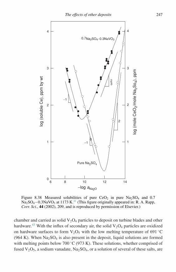
The effects of other deposits 247
log
(sol
uble
Ce)
, ppm
by
wt
0
1
2
3
4
01
2
3
4
log
(mol
e C
eO2/
mol
e N
a 2S
o 4),
ppm
6 8 10 12 14
−log aNa2O
0.7Na2SO4−0.3NaVO3
2_3
−1
−1
2
Pure Na2SO4
Figure 8.38 Measured solubilities of pure CeO2 in pure Na2SO4 and 0.7Na2SO4−0.3NaVO3 at 1173 K.41 (This figure originally appeared in: R. A. Rapp,Corr. Sci., 44 (2002), 209, and is reproduced by permission of Elsevier.)
chamber and carried as solid V2O4 particles to deposit on turbine blades and otherhardware.43 With the influx of secondary air, the solid V2O4 particles are oxidizedon hardware surfaces to form V2O5 with the low melting temperature of 691 ◦C(964 K). When Na2SO4 is also present in the deposit, liquid solutions are formedwith melting points below 700 ◦C (973 K). These solutions, whether comprised offused V2O5, a sodium vanadate, Na2SO4, or a solution of several of these salts, are
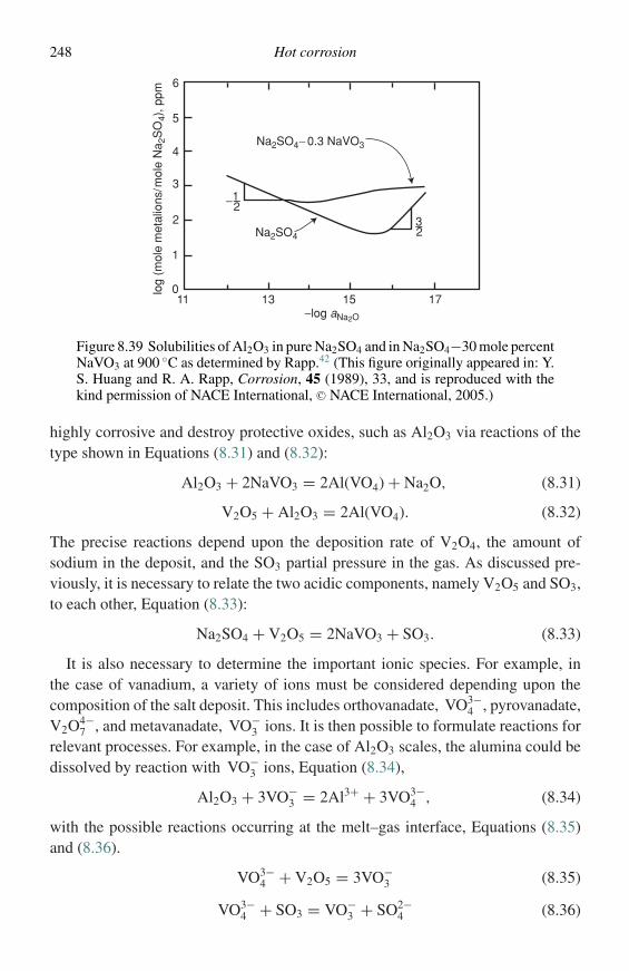
248 Hot corrosion
Na2SO4− 0.3 NaVO3
3–2
−1–2
Na2SO4
11 13 15 170
1
2
3
4
5
6
−log aNa2O
log
(mol
e m
etal
ions
/mol
e N
a 2S
O4)
, ppm
Figure 8.39 Solubilities of Al2O3 in pure Na2SO4 and in Na2SO4−30 mole percentNaVO3 at 900 ◦C as determined by Rapp.42 (This figure originally appeared in: Y.S. Huang and R. A. Rapp, Corrosion, 45 (1989), 33, and is reproduced with thekind permission of NACE International, C© NACE International, 2005.)
highly corrosive and destroy protective oxides, such as Al2O3 via reactions of thetype shown in Equations (8.31) and (8.32):
Al2O3 + 2NaVO3 = 2Al(VO4) + Na2O, (8.31)
V2O5 + Al2O3 = 2Al(VO4). (8.32)
The precise reactions depend upon the deposition rate of V2O4, the amount ofsodium in the deposit, and the SO3 partial pressure in the gas. As discussed pre-viously, it is necessary to relate the two acidic components, namely V2O5 and SO3,to each other, Equation (8.33):
Na2SO4 + V2O5 = 2NaVO3 + SO3. (8.33)
It is also necessary to determine the important ionic species. For example, inthe case of vanadium, a variety of ions must be considered depending upon thecomposition of the salt deposit. This includes orthovanadate, VO3−
4 , pyrovanadate,V2O4−
7 , and metavanadate, VO−3 ions. It is then possible to formulate reactions for
relevant processes. For example, in the case of Al2O3 scales, the alumina could bedissolved by reaction with VO−
3 ions, Equation (8.34),
Al2O3 + 3VO−3 = 2Al3+ + 3VO3−
4 , (8.34)
with the possible reactions occurring at the melt–gas interface, Equations (8.35)and (8.36).
VO3−4 + V2O5 = 3VO−
3 (8.35)
VO3−4 + SO3 = VO−
3 + SO2−4 (8.36)
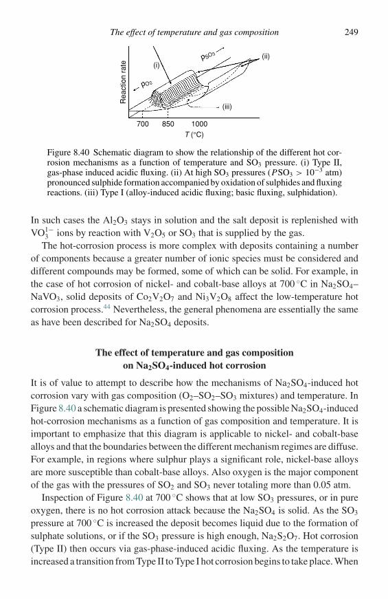
The effect of temperature and gas composition 249
p SO3
p O2
(i)(ii)
(iii)
700 850 1000
T (°C)
Rea
ctio
n ra
te
Figure 8.40 Schematic diagram to show the relationship of the different hot cor-rosion mechanisms as a function of temperature and SO3 pressure. (i) Type II,gas-phase induced acidic fluxing. (ii) At high SO3 pressures (PSO3 > 10−3 atm)pronounced sulphide formation accompanied by oxidation of sulphides and fluxingreactions. (iii) Type I (alloy-induced acidic fluxing; basic fluxing, sulphidation).
In such cases the Al2O3 stays in solution and the salt deposit is replenished withVO1−
3 ions by reaction with V2O5 or SO3 that is supplied by the gas.The hot-corrosion process is more complex with deposits containing a number
of components because a greater number of ionic species must be considered anddifferent compounds may be formed, some of which can be solid. For example, inthe case of hot corrosion of nickel- and cobalt-base alloys at 700 ◦C in Na2SO4–NaVO3, solid deposits of Co2V2O7 and Ni3V2O8 affect the low-temperature hotcorrosion process.44 Nevertheless, the general phenomena are essentially the sameas have been described for Na2SO4 deposits.
The effect of temperature and gas compositionon Na2SO4-induced hot corrosion
It is of value to attempt to describe how the mechanisms of Na2SO4-induced hotcorrosion vary with gas composition (O2–SO2–SO3 mixtures) and temperature. InFigure 8.40 a schematic diagram is presented showing the possible Na2SO4-inducedhot-corrosion mechanisms as a function of gas composition and temperature. It isimportant to emphasize that this diagram is applicable to nickel- and cobalt-basealloys and that the boundaries between the different mechanism regimes are diffuse.For example, in regions where sulphur plays a significant role, nickel-base alloysare more susceptible than cobalt-base alloys. Also oxygen is the major componentof the gas with the pressures of SO2 and SO3 never totaling more than 0.05 atm.
Inspection of Figure 8.40 at 700 ◦C shows that at low SO3 pressures, or in pureoxygen, there is no hot corrosion attack because the Na2SO4 is solid. As the SO3
pressure at 700 ◦C is increased the deposit becomes liquid due to the formation ofsulphate solutions, or if the SO3 pressure is high enough, Na2S2O7. Hot corrosion(Type II) then occurs via gas-phase-induced acidic fluxing. As the temperature isincreased a transition from Type II to Type I hot corrosion begins to take place. When
250 Hot corrosion
the SO3 pressure is low, or in pure oxygen at temperatures above the melting pointof Na2SO4 (884 ◦C) Type I hot corrosion occurs via basic fluxing or sulphidation.In the case of superalloys with elements such as Mo, W, or V alloy-induced acidicfluxing is also prevalent. At all temperatures between 700 and 1000 ◦C as theSO3 pressure is increased heavy sulphide formation in the alloy begins to become adominant feature in all of the alloys. Nickel-base alloys are more susceptible to suchconditions than cobalt-base alloys. In some alloys the observed increase in corrosionappears to result from the oxidation of these sulphides. Udimet is an example ofthis type of degradation. For others, the sulphides permit rapid transport of metalout through the corrosion product, which is accompanied by inward movement ofSO3 through the outer sulphate layer. Nickel is an example of this latter type of hotcorrosion attack.
Test methods
Finally, it is important to discuss the type of experiments that should be performed todetermine the hot corrosion properties of metals and alloys. The answer, of course,is that the test should duplicate the conditions for the application of interest. How-ever, this is not always possible, because the operating conditions may not be welldefined and they may be difficult to simulate experimentally. When this is the case,it is important to document the degradation microstructures from service hardware,and then attempt to develop similar microstructures using selected conditions inlaboratory experiments. Care must be exercised in using this approach, however,because a full understanding of the effects of all the experimental variables maynot be ascertained. This is especially the case where different combinations of theimportant experimental variables are considered. For example, in the case of gasturbines the early work was done by coating specimens with Na2SO4 and oxidizingin air at 900 ◦C, or by using burner rigs, with the objectives of developing degrada-tion microstructures similar to those in service, where the service experience cameprimarily from aircraft gas turbines. As gas turbines began to be used in marineenvironments it was necessary to use SO3 at temperatures lower than 900 ◦C inthe laboratory experiments, and to duct the burner rigs in order to develop thedegradation microstructures observed in marine service. The importance of incor-porating SO3 into the test conditions was only appreciated after low-temperaturehot corrosion became a problem.
References
1. F. S. Pettit and C. S. Giggins, ‘Hot corrosion’. In Superalloys II, eds. C. T. Sims, N.S. Stoloff, and W. C. Hagel, New York, NY, John Wiley & Sons, 1987.
2. J. Stringer, Ann. Rev. Mater. Sci., 7 (1976), 477.3. Y. S. Zhang and R. A. Rapp, J. Met., 46 (December) (1994), 47.
References 251
4. J. Stringer, in High Temperature Corrosion, NACE-6, ed. R. A. Rapp, Houston, TX,National Association of Corrosion Engineers, 1983, p. 389.
5. S. R. J. Saunders, ‘Corrosion in the presence of melts and solids’. In Guidelines forMethods of Testing and Research in High Temperature Corrosion, eds. H. J. Grabkeand D. B. Meadowcroft, London, The Institute of Materials, 1995, p. 85.
6. F. S. Pettit, ‘Molten Salts’. In Corrosion Tests and Standards, ed. R. Baboian, ASTMManual Series: Manual 20 Philadelphia, PA, American Society for Testing andMaterials.
7. D. A. Shifler, ‘High temperature gaseous corrosion testing’, ASM Handbook,Materials Park, OH, ASM International, 2003, vol. 13A, p. 650.
8. R. H. Barkalow and G. W. Goward, in High Temperature Corrosion, NACE-6, ed. R.A. Rapp, Houston, Texas, National Association of Corrosion Engineers Houston,TX, (1983), p. 502.
9. N. S. Bornstein and W. P. Allen, Mater. Sci. Forum, 251–254 (1997), 127.10. J. G. Tschinkel, Corrosion, 28 (1972), 161.11. R. E. Andersen, J. Electrochem. Soc., 128 (1979), 328.12. K. L. Luthra, Met. Trans., 13A (1982), 1853.13. J. M. Quets and W. H. Dresher, J. Mater., 4 (1969), 583.14. D. K. Gupta and R. A. Rapp, J. Electrochem. Soc., 127 (1980), 2194.15. P. D. Jose, D. K. Gupta, and R. A. Rapp, J. Electrochem. Soc., 132 (1985), 73.16. Z. S. Zhang and R. A. Rapp, J. Electrochem. Soc., 132 (1985), 734; 2498.17. R. A. Rapp, Corrosion, 42 (1986), 568.18. M. L. Dearnhardt and K. H. Stern, J. Electrochem. Soc., 129 (1982), 2228.19. R. A. Rapp and K. S. Goto, ‘The hot corrosion of metals by molten salts’. In Molten
Salts, eds. J. Braunstein and J. R. Selman, Pennington, New Jersey, ElectrochemicalSociety, 1981, p. 81.
20. D. A. Shores, in High Temperature Corrosion, NACE-6, ed. R. A. Rapp, Houston,Texas, National Association of Corrosion Engineers, 1983, p. 493.
21. N. S. Bornstein and M. A. DeCrescente, Trans. Met. Soc. AIME, 245 (1969), 1947.22. N. S. Bornstein and M. A. DeCrescente, Met. Trans., 2 (1971), 2875.23. J. A. Goebel and F. S. Pettit, Met. Trans., 1 (1970), 1943.24. D. R. Chang, R. Nemoto, and J. B. Wagner, Jr., Met. Trans., 7A (1976), 803.25. M. R. Wootton and N. Birks, Corr. Sci., 12, (1972), 829.26. N. Otsuka and R. A. Rapp, J. Electrochem. Soc., 137 (1990), 46.27. K. P. Lillerud and P. Kofstad, Oxid. Met., 21 (1984), 233.28. Y. Zhang, J. Electrochem. Soc., 137 (1990), 53.29. R. A. Rapp, Corr. Sci., 44 (2002), 209.30. A. K. Misra, Oxid. Met., 25 (1986), 129.31. A. K. Misra, J. Electrochem. Soc., 133 (1986), 1038.32. G. C. Fryburg, F. J. Kohl, C. A. Stearns, and W. L. Fielder, J. Electrochem. Soc., 129
(1982), 571.33. K. L. Luthra and D. A. Shores, J. Electrochem. Soc., 127 (1980), 2202.34. K. L. Luthra, Met. Trans., 13A (1982), 1647; 1843.35. R. H. Barkalow and F. S. Pettit, ‘On Oxidation Mechanisms for Hot Corrosion of
CoCrAlY Coatings in Marine Gas Turbines,’ Proceedings of the 14th Conference onGas Turbine Materials in a Marine Environment, Naval Sea Systems Command,Annapolis, MD, 1979, p. 493.
36. K. T. Chiang, F. S. Pettit, and G. H. Meier, ‘Low temperature hot corrosion.’ HighTemperature Corrosion, NACE-6, ed. R. A. Rapp, Houston, Texas, NationalAssociation of Corrosion Engineers, 1983, p. 519.

252 Hot corrosion
37. J. A. Goebel and F. S. Pettit, Met. Trans., 1 (1970), 3421.38. P. Kofstad and G. Akesson, Oxid. Met., 14 (1980), 301.39. J. B. Johnson, J. R. Nicholls, R. C. Hurst, and P. Hancock, Corr. Sci., 18 (1978), 543.40. M. G. Fontana and N. D. Greene, Corrosion Engineering, 2nd edn, New York,
McGraw Hill, 1978, p. 67.41. Y. Zhang and R. A. Rapp, Corrosion, 43 (1987), 348.42. Y. S. Huang and R. A. Rapp, Corrosion, 45 (1989), 33.43. C. G. Stearns and D. Tidy, J. Inst. Energy, 56 (1983), 12.44. B. M. Warnes, The influence of vanadium on the sodium sulfate induced hot
corrosion of thermal barrier coating materials, Ph.D. Dissertation, University ofPittsburgh, PA, 1990.
9
Erosion–corrosion of metals in oxidizing atmospheres
Introduction
Under many service situations, materials are exposed to high-temperature gasstreams. A gas stream can entrain solid particles, picking up larger particles athigher speeds. In fact it is probable that a particle-free gas flow can only be pro-vided under the most carefully contrived laboratory conditions. In most practicalcases, gas streams will contain solid particles. Good examples of this are foundin gas turbines, oil refining and reforming, as well as in power generation. Thischapter will address the ways in which the oxidation and solid-particle erosion ofmetals proceed simultaneously and interact.
Erosion of materials
To understand how erosion and oxidation interact, it is necessary to understand howmetals and oxides erode. Previous work into the erosion of metals and ceramicsat room temperature1–4 has shown that the erosion of ductile material involvesplastic deformation, cutting, plowing, and fatigue. These mechanisms can occurby the impact of a single particle, as in the case of cutting, or may require severalsubsequent impacts as in the cases of plowing and fatigue. Brittle materials, on theother hand, erode by the introduction of intersecting brittle crack systems.5 Mostof the metals in use respond in a basically ductile manner at high temperatures. Theoxides that arise from oxidation can be either quite ductile (wustite, nickel oxide,etc.) or quite brittle (alumina, chromia, etc.). Depending on the oxide and thecircumstances, the oxide scale can be deformed plastically by the erosive impacts;alternatively the oxide could spall under impact.
Ductile and brittle materials respond quite differently to variations in the angleof attack of the erodent on the substrate. The rate of erosion of a brittle materialincreases with the angle of attack, reaching a maximum at normal incidence, as
253
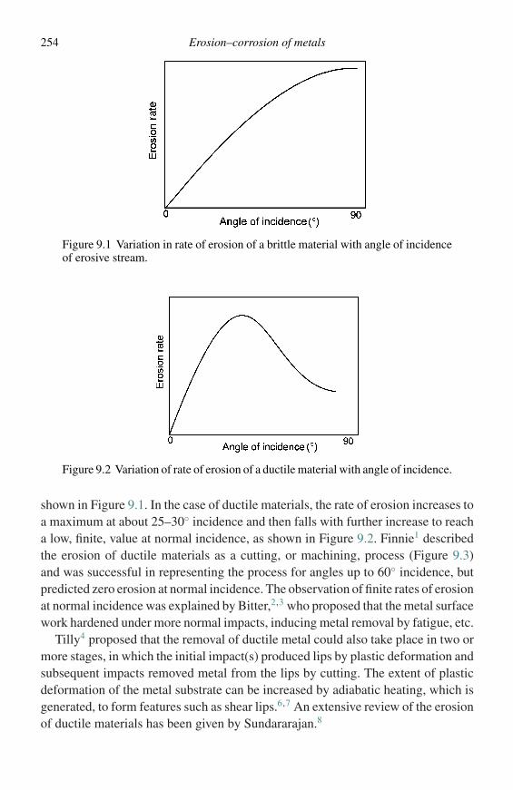
254 Erosion–corrosion of metals
Figure 9.1 Variation in rate of erosion of a brittle material with angle of incidenceof erosive stream.
Figure 9.2 Variation of rate of erosion of a ductile material with angle of incidence.
shown in Figure 9.1. In the case of ductile materials, the rate of erosion increases toa maximum at about 25–30◦ incidence and then falls with further increase to reacha low, finite, value at normal incidence, as shown in Figure 9.2. Finnie1 describedthe erosion of ductile materials as a cutting, or machining, process (Figure 9.3)and was successful in representing the process for angles up to 60◦ incidence, butpredicted zero erosion at normal incidence. The observation of finite rates of erosionat normal incidence was explained by Bitter,2,3 who proposed that the metal surfacework hardened under more normal impacts, inducing metal removal by fatigue, etc.
Tilly4 proposed that the removal of ductile metal could also take place in two ormore stages, in which the initial impact(s) produced lips by plastic deformation andsubsequent impacts removed metal from the lips by cutting. The extent of plasticdeformation of the metal substrate can be increased by adiabatic heating, which isgenerated, to form features such as shear lips.6,7 An extensive review of the erosionof ductile materials has been given by Sundararajan.8
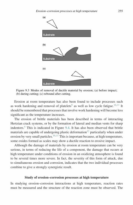
Erosion–corrosion processes at high temperature 255
(a)
(b)
(c)
Figure 9.3 Modes of removal of ductile material by erosion; (a) before impact;(b) during cutting; (c) rebound after cutting.
Erosion at room temperature has also been found to include processes suchas work hardening and removal of platelets9 as well as low cycle fatigue.10,11 Itshould be remembered that processes that involve work hardening will become lesssignificant as the temperature increases.
The erosion of brittle materials has been described in terms of interactingHertzian crack systems, or by the formation of lateral and median vents for sharpindentors.5 This is indicated in Figure 9.4. It has also been observed that brittlematerials are capable of undergoing plastic deformation12 particularly when undererosion by very small particles.10,11 This is important because, at high temperature,some oxides formed as scales may show a ductile reaction to erosive impact.
Although the damage of materials by erosion at room temperature can be veryserious, in terms of reducing the life of a component, the damage that occurs athigh temperature under conditions of erosion in an oxidizing atmosphere is foundto be several times more severe. In fact, the severity of this form of attack, dueto simultaneous erosion and corrosion, indicates that the two individual processescombine to give a strongly synergistic result.
Study of erosion–corrosion processes at high temperature
In studying erosion–corrosion interactions at high temperature, reaction ratesmust be measured and the structure of the reaction zone must be observed. The
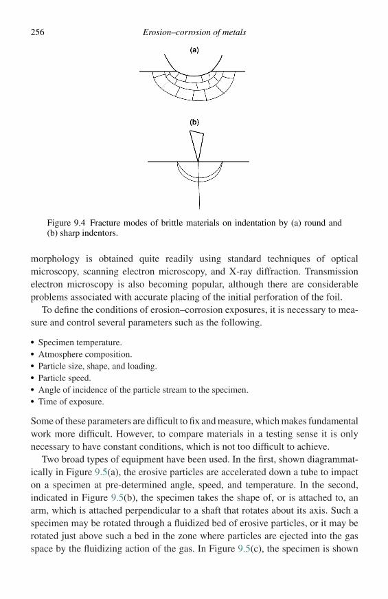
256 Erosion–corrosion of metals
Figure 9.4 Fracture modes of brittle materials on indentation by (a) round and(b) sharp indentors.
morphology is obtained quite readily using standard techniques of opticalmicroscopy, scanning electron microscopy, and X-ray diffraction. Transmissionelectron microscopy is also becoming popular, although there are considerableproblems associated with accurate placing of the initial perforation of the foil.
To define the conditions of erosion–corrosion exposures, it is necessary to mea-sure and control several parameters such as the following.
� Specimen temperature.� Atmosphere composition.� Particle size, shape, and loading.� Particle speed.� Angle of incidence of the particle stream to the specimen.� Time of exposure.
Some of these parameters are difficult to fix and measure, which makes fundamentalwork more difficult. However, to compare materials in a testing sense it is onlynecessary to have constant conditions, which is not too difficult to achieve.
Two broad types of equipment have been used. In the first, shown diagrammat-ically in Figure 9.5(a), the erosive particles are accelerated down a tube to impacton a specimen at pre-determined angle, speed, and temperature. In the second,indicated in Figure 9.5(b), the specimen takes the shape of, or is attached to, anarm, which is attached perpendicular to a shaft that rotates about its axis. Such aspecimen may be rotated through a fluidized bed of erosive particles, or it may berotated just above such a bed in the zone where particles are ejected into the gasspace by the fluidizing action of the gas. In Figure 9.5(c), the specimen is shown
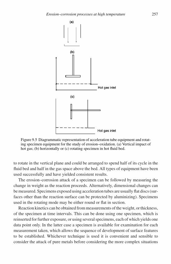
Erosion–corrosion processes at high temperature 257
Figure 9.5 Diagrammatic representation of acceleration tube equipment and rotat-ing specimen equipment for the study of erosion–oxidation. (a) Vertical impact ofhot gas; (b) horizontally or (c) rotating specimen in hot fluid bed.
to rotate in the vertical plane and could be arranged to spend half of its cycle in thefluid bed and half in the gas space above the bed. All types of equipment have beenused successfully and have yielded consistent results.
The erosion–corrosion attack of a specimen can be followed by measuring thechange in weight as the reaction proceeds. Alternatively, dimensional changes canbe measured. Specimens exposed using acceleration tubes are usually flat discs (sur-faces other than the reaction surface can be protected by aluminizing). Specimensused in the rotating mode may be either round or flat in section.
Reaction kinetics can be obtained from measurements of the weight, or thickness,of the specimen at time intervals. This can be done using one specimen, which isreinserted for further exposure, or using several specimens, each of which yields onedata point only. In the latter case a specimen is available for examination for eachmeasurement taken, which allows the sequence of development of surface featuresto be established. Whichever technique is used it is convenient and sensible toconsider the attack of pure metals before considering the more complex situations
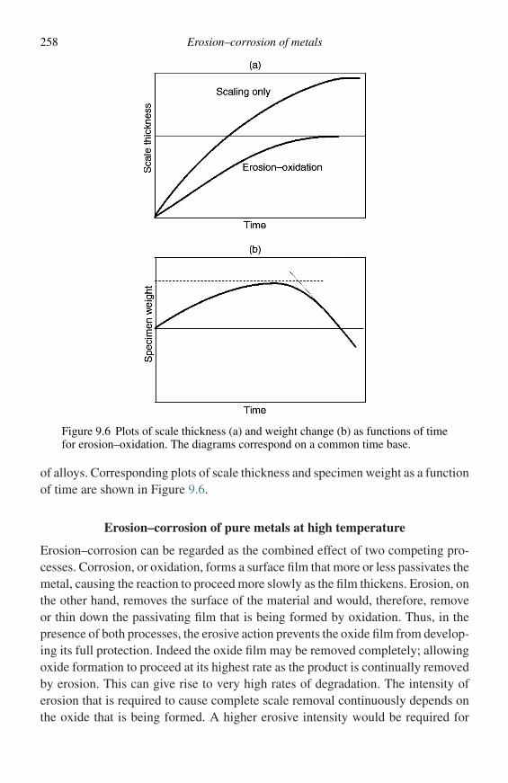
258 Erosion–corrosion of metals
Figure 9.6 Plots of scale thickness (a) and weight change (b) as functions of timefor erosion–oxidation. The diagrams correspond on a common time base.
of alloys. Corresponding plots of scale thickness and specimen weight as a functionof time are shown in Figure 9.6.
Erosion–corrosion of pure metals at high temperature
Erosion–corrosion can be regarded as the combined effect of two competing pro-cesses. Corrosion, or oxidation, forms a surface film that more or less passivates themetal, causing the reaction to proceed more slowly as the film thickens. Erosion, onthe other hand, removes the surface of the material and would, therefore, removeor thin down the passivating film that is being formed by oxidation. Thus, in thepresence of both processes, the erosive action prevents the oxide film from develop-ing its full protection. Indeed the oxide film may be removed completely; allowingoxide formation to proceed at its highest rate as the product is continually removedby erosion. This can give rise to very high rates of degradation. The intensity oferosion that is required to cause complete scale removal continuously depends onthe oxide that is being formed. A higher erosive intensity would be required for
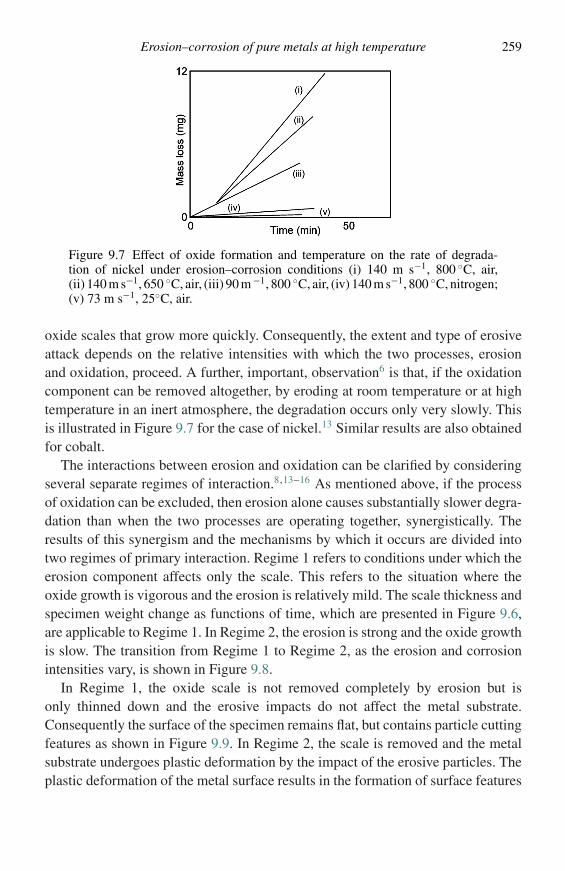
Erosion–corrosion of pure metals at high temperature 259
Figure 9.7 Effect of oxide formation and temperature on the rate of degrada-tion of nickel under erosion–corrosion conditions (i) 140 m s−1, 800 ◦C, air,(ii) 140 m s−1, 650 ◦C, air, (iii) 90 m −1, 800 ◦C, air, (iv) 140 m s−1, 800 ◦C, nitrogen;(v) 73 m s−1, 25◦C, air.
oxide scales that grow more quickly. Consequently, the extent and type of erosiveattack depends on the relative intensities with which the two processes, erosionand oxidation, proceed. A further, important, observation6 is that, if the oxidationcomponent can be removed altogether, by eroding at room temperature or at hightemperature in an inert atmosphere, the degradation occurs only very slowly. Thisis illustrated in Figure 9.7 for the case of nickel.13 Similar results are also obtainedfor cobalt.
The interactions between erosion and oxidation can be clarified by consideringseveral separate regimes of interaction.8,13–16 As mentioned above, if the processof oxidation can be excluded, then erosion alone causes substantially slower degra-dation than when the two processes are operating together, synergistically. Theresults of this synergism and the mechanisms by which it occurs are divided intotwo regimes of primary interaction. Regime 1 refers to conditions under which theerosion component affects only the scale. This refers to the situation where theoxide growth is vigorous and the erosion is relatively mild. The scale thickness andspecimen weight change as functions of time, which are presented in Figure 9.6,are applicable to Regime 1. In Regime 2, the erosion is strong and the oxide growthis slow. The transition from Regime 1 to Regime 2, as the erosion and corrosionintensities vary, is shown in Figure 9.8.
In Regime 1, the oxide scale is not removed completely by erosion but isonly thinned down and the erosive impacts do not affect the metal substrate.Consequently the surface of the specimen remains flat, but contains particle cuttingfeatures as shown in Figure 9.9. In Regime 2, the scale is removed and the metalsubstrate undergoes plastic deformation by the impact of the erosive particles. Theplastic deformation of the metal surface results in the formation of surface features
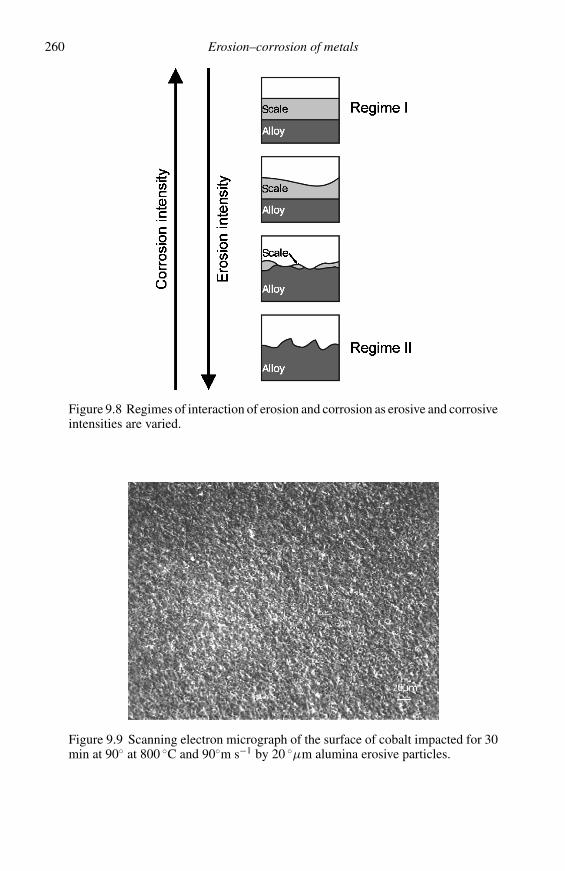
260 Erosion–corrosion of metals
Figure 9.8 Regimes of interaction of erosion and corrosion as erosive and corrosiveintensities are varied.
Figure 9.9 Scanning electron micrograph of the surface of cobalt impacted for 30min at 90◦ at 800 ◦C and 90◦m s−1 by 20 ◦µm alumina erosive particles.

Erosion–corrosion of pure metals at high temperature 261
Figure 9.10 Surface topography developed on eroding nickel in air at 800 ◦C using20 µm alumina particles: (a) impacting at 140 m s−1 at 90◦ for 30 min; and (b)impacting at 90 m s−1 at 30◦ for 30 min.
in relief that can be substantially larger than the erosive particles themselves. Thesesurface features can resemble hills and valleys at normal incidence of the erosiveflow, as shown in Figure 9.10(a), or systems of ripples at oblique incidence, Figure9.10(b).13 It is believed that the component of the erosive flow that is parallel to thesurface is responsible for the alignment of the ripples and for their slow progressionthat is observed to occur across the metal surface.17
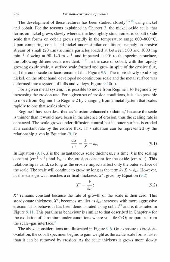
262 Erosion–corrosion of metals
The development of these features has been studied closely13–18 using nickeland cobalt. For the reasons explained in Chapter 3, the nickel oxide scale thatforms on nickel grows slowly whereas the less tightly stoichiometric cobalt oxidescale that forms on cobalt grows rapidly in the temperature range 600–800 ◦C.Upon comparing cobalt and nickel under similar conditions, namely an erosivestream of small (20 µm) alumina particles loaded at between 500 and 1000 mgmin−1, flowing at 90–140 m s−1, and impacted at 90◦ to the specimen surface,the following differences are evident.13,17 In the case of cobalt, with the rapidlygrowing oxide scale, a surface scale formed and grew in spite of the erosive flux,and the outer scale surface remained flat, Figure 9.9. The more slowly oxidizingnickel, on the other hand, developed no continuous scale and the metal surface wasdeformed into a system of hills and valleys, Figure 9.10(a).
For a given metal system, it is possible to move from Regime 1 to Regime 2 byincreasing the erosion rate. For a given set of erosion conditions, it is also possibleto move from Regime 1 to Regime 2 by changing from a metal system that scalesrapidly to one that scales slowly.
Regime 1 has been described as ‘erosion-enhanced oxidation,’ because the scaleis thinner than it would have been in the absence of erosion, thus the scaling rate isenhanced. The scale grows under diffusion control but its outer surface is erodedat a constant rate by the erosive flux. This situation can be represented by therelationship given in Equation (9.1):
dX
dt= k
X− keo. (9.1)
In Equation (9.1), X is the instantaneous scale thickness, t is time, k is the scalingconstant (cm2 s−1) and keo is the erosion constant for the oxide (cm s−1). Thisrelationship is valid, so long as the erosive impacts affect only the outer surface ofthe scale. The scale will continue to grow, so long as the term k/X > keo. However,as the scale grows it reaches a critical thickness, X∗, given by Equation (9.2),
X∗ = k
keo; (9.2)
X∗ remains constant because the rate of growth of the scale is then zero. Thissteady-state thickness, X∗, becomes smaller as keo increases with more aggressiveerosion. This behaviour has been demonstrated using cobalt19 and is illustrated inFigure 9.11. This paralinear behaviour is similar to that described in Chapter 4 forthe oxidation of chromium under conditions where volatile CrO3 evaporates fromthe scale–gas interface.20
The above considerations are illustrated in Figure 9.6. On exposure to erosion–oxidation, the cobalt specimen begins to gain weight as the oxide scale forms fasterthan it can be removed by erosion. As the scale thickens it grows more slowly
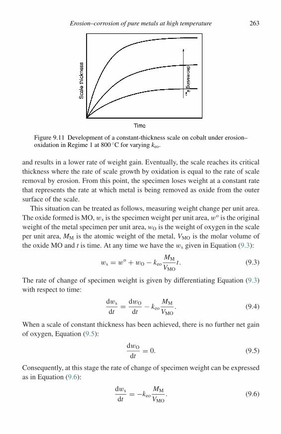
Erosion–corrosion of pure metals at high temperature 263
Figure 9.11 Development of a constant-thickness scale on cobalt under erosion–oxidation in Regime 1 at 800 ◦C for varying keo.
and results in a lower rate of weight gain. Eventually, the scale reaches its criticalthickness where the rate of scale growth by oxidation is equal to the rate of scaleremoval by erosion. From this point, the specimen loses weight at a constant ratethat represents the rate at which metal is being removed as oxide from the outersurface of the scale.
This situation can be treated as follows, measuring weight change per unit area.The oxide formed is MO, ws is the specimen weight per unit area, wo is the originalweight of the metal specimen per unit area, wO is the weight of oxygen in the scaleper unit area, MM is the atomic weight of the metal, VMO is the molar volume ofthe oxide MO and t is time. At any time we have the ws given in Equation (9.3):
ws = wo + wO − keoMM
VMOt. (9.3)
The rate of change of specimen weight is given by differentiating Equation (9.3)with respect to time:
dws
dt= dwO
dt− keo
MM
VMO. (9.4)
When a scale of constant thickness has been achieved, there is no further net gainof oxygen, Equation (9.5):
dwO
dt= 0. (9.5)
Consequently, at this stage the rate of change of specimen weight can be expressedas in Equation (9.6):
dws
dt= −keo
MM
VMO. (9.6)
264 Erosion–corrosion of metals
As the scale develops, there will also be a time when the rate of weight gain of thespecimen is zero, Equation (9.7),
dws
dt= 0, (9.7)
and, from Equation (9.4), Equation (9.8) is obtained:
dwO
dt= keo
MM
VMO. (9.8)
At this point, the rate of gain of weight as oxygen is equal to the rate of weightloss of metal as oxide. The scale continues to thin down, however, and the constantscale thickness is only achieved when Equations (9.5) and (9.6) are satisfied, asshown in Figure 9.6.
Regime 1 has been studied by several groups of workers13–17,19 and an interpre-tation of the mechanism by which the reactions in this regime proceed has beendeveloped.18,21 The basic concept in this interpretation is that the erosive impactsremove a portion of the surface of the protective scale over a ‘footprint’ caused byan individual particle impact.18 During the time between successive impacts at thesame site the scale can form more oxide and ‘heal.’ If the amount of scale formedduring healing is less than that which is removed at each impact, then the scale willthin down.
The value of the erosion constant will vary with the erosion conditions, thusunder strong erosion the actual rate of scale formation will increase as the scalethickness is held to low values. The rate of scale formation is also the rate at whichthe metal degrades by conversion to oxide.
From Equation (9.1) it can be seen that if the rates of oxide formation and erosionare equal, then the scale will remain at constant thickness, X∗, given by Equation(9.2). Clearly, the higher the value of keo, the thinner the scale will be and the fasterthe metal will degrade. Eventually, the erosion process can be made so severe thatthe behaviour pattern moves from Regime 1 to Regime 2, when the erosion beginsto deform the metal surface.
A semi-quantitative analysis of the model for Regime 1 has been given,21 asfollows. It is assumed that all particles are identical, of volume v and density ρ.They are impinged on the specimen of area A at a loading rate of M (g s−1), eachimpact produces a footprint of area a and removes material to a depth d. The timebetween impacts, t∗, for any given site can be written as in Equation (9.9):
t∗ = νρ A
Ma. (9.9)
The volume of scale removed at each impact is ad. Since the impact rate of particleson the surface is M/vρ s−1, the rate of material removal is Mad/vρ cm3 s−1. A
Erosion–corrosion of pure metals at high temperature 265
macroscopic measurement of the erosion rate gives the rate of material removal askeoA. Thus, the depth removed per impact, d, can be obtained, Equation (9.10):
d = keoAνρ
Ma= keot. (9.10)
The time between impacts can be calculated from Equation (9.9) and the depthremoved per impact, d, can be calculated from keo, previously measured for theoxide. The value obtained for d can now be compared with the thickness of oxidethat would be expected to form in the time between impacts. If d is greater thanthe oxide growth, then the scale will become thinner, by the action of erosion. Anexpression for the scale growth can be derived as follows. For the growth of theoxide we have Equations (9.11) or (9.12):
dX
dt= k
X; (9.11)
XdX = k dt ; (9.12)
the latter may be integrated indefinitely to give Equation (9.13):
X2 = 2kt∗ + C. (9.13)
At t∗ = 0, X = X∗ so that Equation (9.14) is obtained,
X2 = X∗2 + 2kt∗, (9.14)
where k is the parabolic scaling constant, X is the scale thickness after time t∗
(time between impacts) from an initial steady-state thickness, X∗, i.e., X = X∗ +d under steady state because d is formed and removed every t∗ seconds. Thus,substituting into Equation (9.14), the steady-state thickness, X∗, may be written as inEquation (9.15):
X∗ = 2kt∗ − d2
2d. (9.15)
If this value is positive, then the reaction produces a limiting scale of finite thicknessand the system is reacting in Regime 1. If the value calculated for X∗ were to benegative then this would mean that the scale is not capable of growing quicklyenough to overcome the effects of erosion and would, therefore, be reacting inRegime 2. Such values have been calculated for the cases of cobalt and nickelunder erosion–oxidation at 700 ◦C.13
The erosion rate constants for nickel oxide, NiO, and cobalt oxide, CoO, at 700◦C in a stream of 20 µm alumina particles flowing at 463 mg min−1, were deter-mined to be 9 × 10⁻⁷ and 3.5 × 10⁻⁷ cm s−1, respectively. The time betweenimpacts for this erosive flow was 10.5 s yielding values of d, the thickness removed
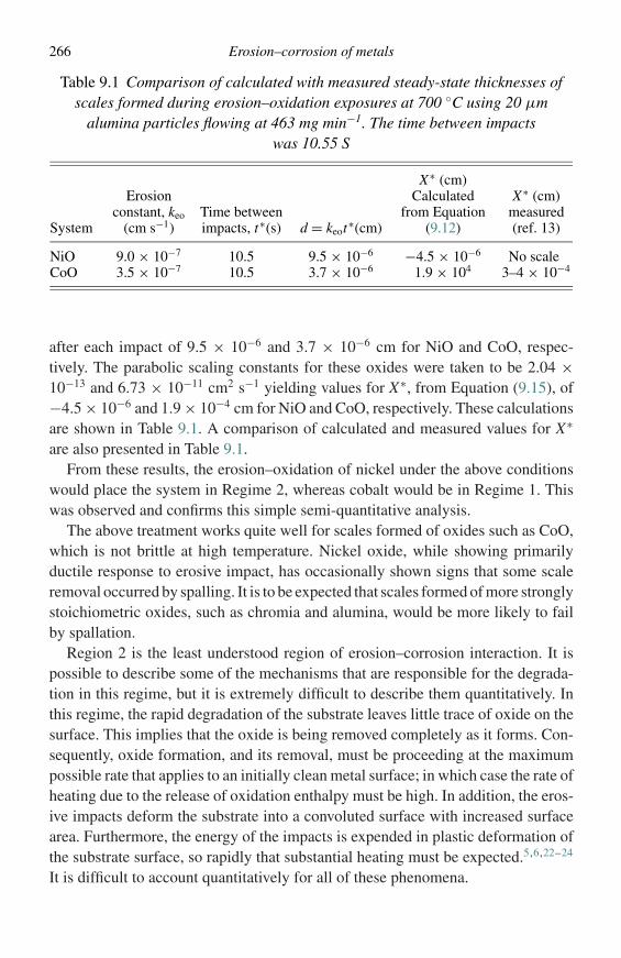
266 Erosion–corrosion of metals
Table 9.1 Comparison of calculated with measured steady-state thicknesses ofscales formed during erosion–oxidation exposures at 700 ◦C using 20 µm
alumina particles flowing at 463 mg min−1. The time between impactswas 10.55 S
System
Erosionconstant, keo
(cm s−1)Time betweenimpacts, t∗(s) d = keot∗(cm)
X∗ (cm)Calculated
from Equation(9.12)
X∗ (cm)measured(ref. 13)
NiO 9.0 × 10⁻⁷ 10.5 9.5 × 10⁻⁶ −4.5 × 10⁻⁶ No scaleCoO 3.5 × 10⁻⁷ 10.5 3.7 × 10⁻⁶ 1.9 × 10⁴ 3–4 × 10⁻⁴
after each impact of 9.5 × 10⁻⁶ and 3.7 × 10⁻⁶ cm for NiO and CoO, respec-tively. The parabolic scaling constants for these oxides were taken to be 2.04 ×10⁻¹³ and 6.73 × 10⁻¹¹ cm2 s−1 yielding values for X∗, from Equation (9.15), of−4.5 × 10⁻⁶ and 1.9 × 10⁻⁴ cm for NiO and CoO, respectively. These calculationsare shown in Table 9.1. A comparison of calculated and measured values for X∗
are also presented in Table 9.1.From these results, the erosion–oxidation of nickel under the above conditions
would place the system in Regime 2, whereas cobalt would be in Regime 1. Thiswas observed and confirms this simple semi-quantitative analysis.
The above treatment works quite well for scales formed of oxides such as CoO,which is not brittle at high temperature. Nickel oxide, while showing primarilyductile response to erosive impact, has occasionally shown signs that some scaleremoval occurred by spalling. It is to be expected that scales formed of more stronglystoichiometric oxides, such as chromia and alumina, would be more likely to failby spallation.
Region 2 is the least understood region of erosion–corrosion interaction. It ispossible to describe some of the mechanisms that are responsible for the degrada-tion in this regime, but it is extremely difficult to describe them quantitatively. Inthis regime, the rapid degradation of the substrate leaves little trace of oxide on thesurface. This implies that the oxide is being removed completely as it forms. Con-sequently, oxide formation, and its removal, must be proceeding at the maximumpossible rate that applies to an initially clean metal surface; in which case the rate ofheating due to the release of oxidation enthalpy must be high. In addition, the eros-ive impacts deform the substrate into a convoluted surface with increased surfacearea. Furthermore, the energy of the impacts is expended in plastic deformation ofthe substrate surface, so rapidly that substantial heating must be expected.5,6,22–24
It is difficult to account quantitatively for all of these phenomena.
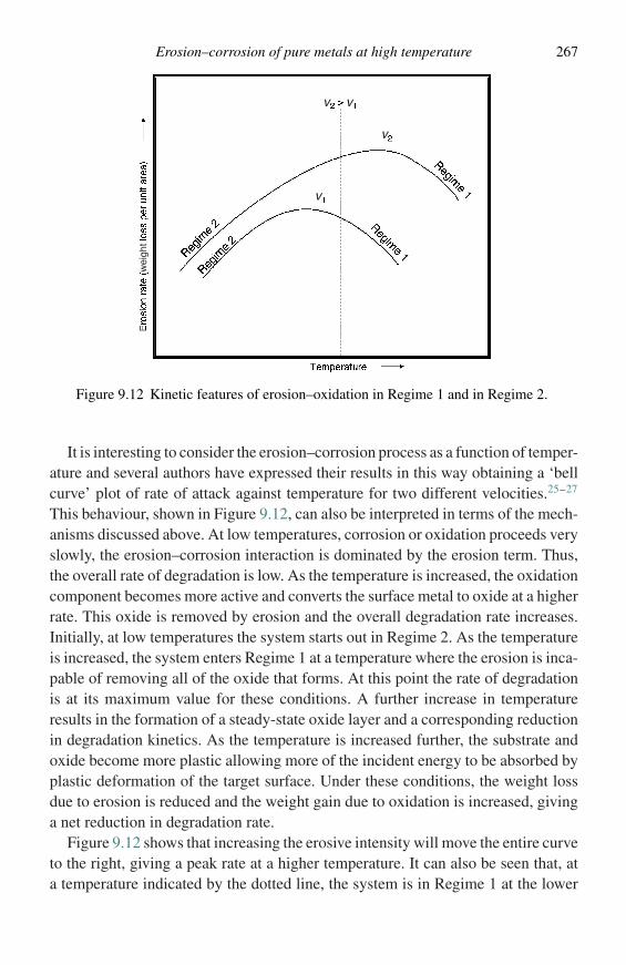
Erosion–corrosion of pure metals at high temperature 267
wei
ght
v
v
v
v
Figure 9.12 Kinetic features of erosion–oxidation in Regime 1 and in Regime 2.
It is interesting to consider the erosion–corrosion process as a function of temper-ature and several authors have expressed their results in this way obtaining a ‘bellcurve’ plot of rate of attack against temperature for two different velocities.25–27
This behaviour, shown in Figure 9.12, can also be interpreted in terms of the mech-anisms discussed above. At low temperatures, corrosion or oxidation proceeds veryslowly, the erosion–corrosion interaction is dominated by the erosion term. Thus,the overall rate of degradation is low. As the temperature is increased, the oxidationcomponent becomes more active and converts the surface metal to oxide at a higherrate. This oxide is removed by erosion and the overall degradation rate increases.Initially, at low temperatures the system starts out in Regime 2. As the temperatureis increased, the system enters Regime 1 at a temperature where the erosion is inca-pable of removing all of the oxide that forms. At this point the rate of degradationis at its maximum value for these conditions. A further increase in temperatureresults in the formation of a steady-state oxide layer and a corresponding reductionin degradation kinetics. As the temperature is increased further, the substrate andoxide become more plastic allowing more of the incident energy to be absorbed byplastic deformation of the target surface. Under these conditions, the weight lossdue to erosion is reduced and the weight gain due to oxidation is increased, givinga net reduction in degradation rate.
Figure 9.12 shows that increasing the erosive intensity will move the entire curveto the right, giving a peak rate at a higher temperature. It can also be seen that, ata temperature indicated by the dotted line, the system is in Regime 1 at the lower
268 Erosion–corrosion of metals
erosion rate, but in Regime 2 at the higher erosion rate. The increase in erosion ratecould be achieved simply by increasing the particle velocity.
Erosion–corrosion of alloys
The erosion–corrosion of alloys follows that of pure metals but there are someimportant differences.
� Several oxides may form.� Oxides formed initially may be removed and different oxides may form.� Concentration gradients may form in the alloy.� Alloys are usually stronger than pure metals and less energy may be absorbed due to
thinner deformation zones being formed.
It has been seen that most of the degradation caused by erosion–corrosion at hightemperatures is due to the formation and removal of surface oxide scale. The directremoval of metal by erosion plays a relatively minor role. Thus, alloys that formslow-growing, protective, oxide scales would be expected to degrade more slowlyunder erosion–corrosion than alloys whose scales form more rapidly. This has beenreported28 for cases where the erosive intensity was very low. However, there aretwo circumstances that are capable of defeating this expectation. The first is that,as an oxide scale is removed and reforms on an alloy, it draws the metal formingthe most protective oxide scale from the alloy, and forms a diffusion gradient in thealloy surface. In this case the concentration of the protective metal at the surfacewill fall with time and will eventually no longer be able to support formation ofthis protective oxide. This is similar to the situation with persistent spalling. Thesecond circumstance is that, under erosion, the protective oxide that forms on thealloy surface is unable to grow laterally to form complete coverage of the surface.In this case, the alloy surface is held by the erosion in a state of extended transientoxidation, when all oxides that are thermodynamically capable of forming do so.Since the major alloy partner is usually a metal such as iron or nickel that forms arapidly growing oxide, this situation is expected to result in rapid degradation rates,in spite of the presence in the alloy of elements that normally provide a passivatingoxide layer.
This type of behaviour has been observed29 for the nickel–chromium alloy sys-tem. In this work, pure nickel, Ni–20 wt% Cr and Ni-30 wt% Cr alloys were exposedto erosion–corrosion at 700 and 800 ◦C. An erosive stream, loaded at 400 mg min−1
of 20 µm alumina particles and flowing at 75 and 125 m s−1, was used to impactnormally on the specimens. Under simple oxidation in air at these temperatures, thealloys both developed protective scales of chromia and showed very low rates of
Erosion–corrosion of alloys 269
Figure 9.13 Effect of alloying with chromium on the erosion–oxidation kineticsof nickel exposed to an erosive stream at 90◦ incidence, 700 ◦C and 75 m s−1 Ni(---); Ni–30 wt% Cr (– –); Ni–20 wt% Cr(—).
attack. Under erosion–corrosion conditions however, both alloys degraded at highrates that were comparable, or even identical, to the rate at which the pure nickelwas attacked. The results are shown in Figure 9.13. Both nickel oxide and chromiawere found to exist on the eroded surface but there was no trace of the spinel. Thisshows that these oxides were being removed rapidly, since NiO and Cr2O3 werenot present for sufficient time to form spinel. These results were interpreted byproposing that the erosive stream prevents the formation of a continuous layer ofchromia by removing the oxide faster than it can spread laterally. These specimenswere described as being in a state of ‘erosion-maintained transient oxidation’. Thismechanism implies that it would be difficult for protective scales to form and persiston alloys in the presence of erosion. Consequently, the oxidation behaviour of analloy in the absence of erosion cannot be used as a guide to its behaviour undererosion–oxidation at high temperature.
270 Erosion–corrosion of metals
References
1. I. Finnie, Wear, 3 (1960), 87.2. J. G. Bitter, Wear, 6 (1963), 5.3. J. G. Bitter, Wear, 6 (1963), 169.4. G. P. Tilly, Erosion caused by impact of solid particles. In Treatise on Materials
Science and Technology, ed., C. M. P. Reese, New York, Academic Press, 1979, p.287.
5. I. Finnie and S. Vaidyanathan, ‘Initiation and propagation of hertzian ring cracks.’ InFracture Mechanics of Ceramics, eds., R. C. Bradt, D. P. H. Hasselman, and F. F.Lange, New York, Plenum Press, 1974, p. 231.
6. P. G. Shewmon, Wear, 68 (1981), 254.7. I. M. Hutchings, Wear, 35 (1975), 371.8. G. Sundararajan, Wear of Materials, Orlando, FL, ASME, 1991, p. 111.9. R. Bellman and A. V. Levy, Wear, 70 (1981), 1.
10. G. Sundararajan and P. G. Shewmon, Wear, 84 (1983), 237.11. I. M. Hutchings, Wear, 70 (1981), 269.12. A. G. Evans and T. R. Wilshaw, Acta Met., 24 (1976), 939.13. C. T. Kang, F. S. Pettit, and N. Birks, Met. Trans., A18 (1987), 1785.14. S. Hogmark, A. Hammersten, and S. Soderberg, On the combined effects of erosion
and corrosion. Proceedings of the 6th International Conference on Erosion by Liquidand Solid Impact, J. E. Field and N. S. Corney, eds., Cambridge, 1983, p. 37.
15. D. M. Rishel, N. Birks, and F. S. Pettit, Mat. Sci. Eng., A143 (1991), 197.16. G. Sundararajan, Proceedings of the Conference on Corrosion–Erosion–Wear of
Materials at High Temperature, ed. A. V. Levy, Houstan, TX, NACE, 1991, p. 11–1.17. S. L. Chang, F. S. Pettit, and N. Birks, Oxid. Met., 34 (1990), 23.18. V. J. Sethi and I. G. Wright, Proceedings of the Conference on
Corrosion–Erosion–Wear of Materials at High Temperatures, ed. A. V. Levy,Houstan, TX, NACE, 1991, p. 18-1.
19. S. L. Chang, F. S. Pettit, and N. Birks, Oxid. Met., 34 (1990), 47.20. C. S. Tedmon, J. Electrochem. Soc., 113 (1966), 766.21. N. Birks, F. S. Pettit, and B. Peterson, Mat. Sci. Forum, 251–254, (1997), 475.22. S. L. Chang, Ph.D. Thesis, University of Pittsburgh, PA, 1987.23. R. A. Doyle and A. Ball, Wear, 151 (1991), 87.24. I. M. Hutchings and A. V. Levy, Wear, 131 (1989), 105.25. M. M. Stack, F. H. Stott, and G. C. Wood, Corr. Sci., 33 (1992), 965.26. D. J. Hall and S. R. J. Saunders, High Temperature Materials for Power Engineering,
Liege, Belgium, Kluwer Academic Publishers, 1990.27. B. Q. Wang, G. Q. Geng, and A. V. Levy, Wear, 159 (1992), 233.28. A. V. Levy, Solid Particle Erosion–Corrosion of Materials, Materials Park, OH,
ASM International, 1995.29. R. J. Link, N. Birks, F. S. Pettit, and F. Dethorey, Oxid. Met., 49 (1998), 213.
10
Protective coatings
Introduction
Coatings have been used for centuries for embellishment or for protection of asubstrate that is adequate in all other ways, usually providing shape, stiffness, orstrength. The greatest use of coatings has been at room temperature by the jewellryindustry for appearance, for ceramics by enamelling to improve appearance andprovide impermeability, and by the automobile industry for corrosion protection.In these cases, a very high degree of success has been achieved.
In the use of coatings at high temperatures, the aim is either to protect the surfaceof an inexpensive, but degradable material, as in the use of coextruded tubing forheat exchangers, or to protect the surface of an alloy that has been developedfor strength but does not have sufficient intrinsic resistance to high-temperaturecorrosion. Typical applications consist of power generation using steam boilers,which are usually fired by fossil fuel; and in gas turbines, which are used for aircraftor marine propulsion, or are land based for power generation. In recent years, theuse of ceramic coatings as insulators, thermal-barrier coatings, has also becomeimportant for limiting the degradation of alloys, particularly in gas turbines. Thevarious types of coatings are described extensively in ref. 1.
This chapter is organized to give an overview of the fabrication, use, and degra-dation of the various types of coatings that are available for use in high-temperaturesystems.
Types of coating systems
Diffusion coatings
In diffusion coating, the substrate surface is enriched in an element that will providehigh-temperature corrosion resistance. Typical elements are chromium (chromiz-ing), aluminium (aluminizing), or silicon (siliconizing). The substrate is involved
271
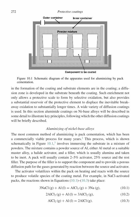
272 Protective coatings
Figure 10.1 Schematic diagram of the apparatus used for aluminizing by packcementation.
in the formation of the coating and substrate elements are in the coating; a diffu-sion zone is developed in the substrate beneath the coating. Such enrichment notonly allows a protective scale to form by selective oxidation, but also providesa substantial reservoir of the protective element to displace the inevitable break-away oxidation to substantially longer times. A wide variety of diffusion coatingsis used. In this section aluminide coatings on Ni-base alloys will be described insome detail to illustrate key principles, following which the other diffusion coatingswill be briefly described.
Aluminizing of nickel-base alloys
The most common method of aluminizing is pack cementation, which has beena commercially viable process for many years.2 This process, which is shownschematically in Figure 10.1,3 involves immersing the substrate in a mixture ofpowders. The mixture contains a powder source of Al, either Al metal or a suitablemaster alloy, a halide activator, and a filler, which is usually alumina and takento be inert. A pack will usually contain 2–5% activator, 25% source and the restfiller. The purpose of the filler is to support the component and to provide a porousdiffusion path for the gases generated by reaction between the source and activator.
The activator volatilizes within the pack on heating and reacts with the sourceto produce volatile species of the coating metal. For example, in NaCl-activatedpacks, the reactions shown in Equations (10.1)–(10.3) take place:
3NaCl (g) + Al (l) = AlCl3 (g) + 3Na (g), (10.1)
2AlCl3 (g) + Al (l) = 3AlCl2 (g), (10.2)
AlCl2 (g) + Al (l) = 2AlCl (g). (10.3)

Types of coating systems 273
The relative partial pressures of the aluminium chlorides will be determined by theactivity of Al in the source, the amount of activator used, and temperature. Thepack is usually held under a gas such as argon to minimize oxidation of the sourceand substrate.
The volatile species diffuse through the pack to the substrate surface where depo-sition reactions take place. The mixture of volatile gas species reflects the activityof aluminium that exists in the source. The component to be coated represents alow-activity sink for the aluminium so that various deposition reactions, includingthose given in Equations (10.4)–(10.8), are possible.
Disproportionation 2AlCl (g) = Al + AlCl2 (g) (10.4)
3AlCl2 (g) = Al + 2AlCl3 (g) (10.5)
Displacement AlCl2 (g) + Ni = Al + NiCl2 (g) (10.6)
Direct reduction AlCl3 (g) = Al + 3
2Cl2 (g) (10.7)
And, for activators which contain hydrogen, e.g. NH4Cl, hydrogen reduction occurs,Equation (10.8).
Hydrogen reduction AlCl3(g) + 3
2H2(g) = Al + 3HCl(g) (10.8)
(The underlined symbols refer to species in the solid substrate.) Displacement reac-tions are not significant in the aluminizing of Ni-base alloys but often predominatein processes such as chromizing of iron and steels.4
The activity of Al established at the substrate surface will be determined by theactivity of Al in the source and by the kinetics of transport of the reactive gasesthrough the pack. Both of these factors will be influenced by depletion of Al fromthe source and activator depletion, and hence by the extent to which the pack ventsgases to the surroundings. The transport kinetics during aluminizing have beenanalyzed by Levine and Caves5 and Seigle and coworkers.6–9 The activity of Alwill fix the Al concentration and, therefore, the phases, which form in the coating,as can be seen from the phase diagram in Figure 10.2. Figure 10.310 shows twotypical coatings prepared by pack aluminizing of a Ni-base superalloy. The coatingshown in Figure 10.3(a) was formed at low temperature in a high Al activity packto produce an inward-growing coating. The coating shown in Figure 10.3(b) wasformed at high temperature in a low Al activity pack to form an outward-growingcoating. The formation mechanisms of these coatings are described in detailin ref. 2. Pack cementation has several advantages over other methods of producingdiffusion coatings. One of these is that the pack serves the additional purpose ofsupporting the substrates. This prevents sagging of large parts and some commercial
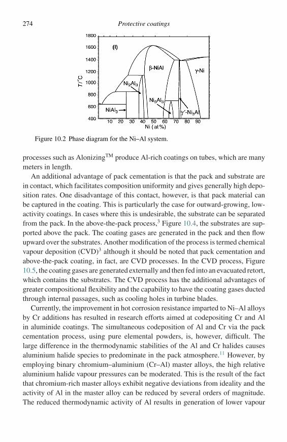
274 Protective coatings
Figure 10.2 Phase diagram for the Ni–Al system.
processes such as AlonizingTM produce Al-rich coatings on tubes, which are manymeters in length.
An additional advantage of pack cementation is that the pack and substrate arein contact, which facilitates composition uniformity and gives generally high depo-sition rates. One disadvantage of this contact, however, is that pack material canbe captured in the coating. This is particularly the case for outward-growing, low-activity coatings. In cases where this is undesirable, the substrate can be separatedfrom the pack. In the above-the-pack process,3 Figure 10.4, the substrates are sup-ported above the pack. The coating gases are generated in the pack and then flowupward over the substrates. Another modification of the process is termed chemicalvapour deposition (CVD)3 although it should be noted that pack cementation andabove-the-pack coating, in fact, are CVD processes. In the CVD process, Figure10.5, the coating gases are generated externally and then fed into an evacuated retort,which contains the substrates. The CVD process has the additional advantages ofgreater compositional flexibility and the capability to have the coating gases ductedthrough internal passages, such as cooling holes in turbine blades.
Currently, the improvement in hot corrosion resistance imparted to Ni–Al alloysby Cr additions has resulted in research efforts aimed at codepositing Cr and Alin aluminide coatings. The simultaneous codeposition of Al and Cr via the packcementation process, using pure elemental powders, is, however, difficult. Thelarge difference in the thermodynamic stabilities of the Al and Cr halides causesaluminium halide species to predominate in the pack atmosphere.11 However, byemploying binary chromium–aluminium (Cr–Al) master alloys, the high relativealuminium halide vapour pressures can be moderated. This is the result of the factthat chromium-rich master alloys exhibit negative deviations from ideality and theactivity of Al in the master alloy can be reduced by several orders of magnitude.The reduced thermodynamic activity of Al results in generation of lower vapour
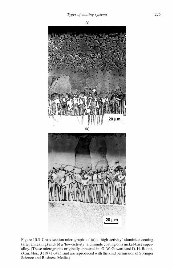
Types of coating systems 275
20 µm
(a)
20 µm
(b)
Figure 10.3 Cross-section micrographs of (a) a ‘high-activity’ aluminide coating(after annealing) and (b) a ‘low-activity’ aluminide coating on a nickel-base super-alloy. (These micrographs originally appeared in: G. W. Goward and D. H. Boone,Oxid. Met., 3 (1971), 475, and are reproduced with the kind permission of SpringerScience and Business Media.)
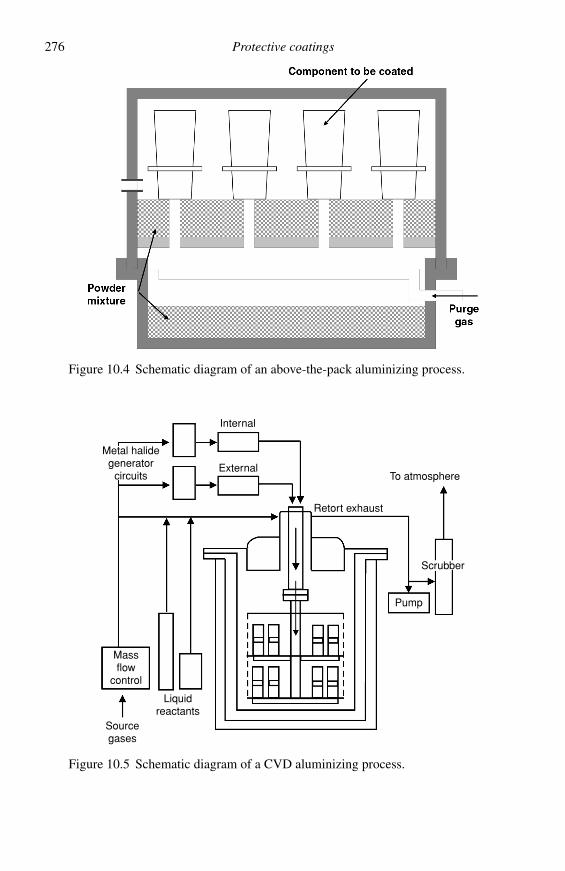
276 Protective coatings
Figure 10.4 Schematic diagram of an above-the-pack aluminizing process.
Metal halidegenerator
circuitsExternal
Internal
Retort exhaust
To atmosphere
Scrubber
Pump
Massflow
control
Liquidreactants
Sourcegases
Figure 10.5 Schematic diagram of a CVD aluminizing process.
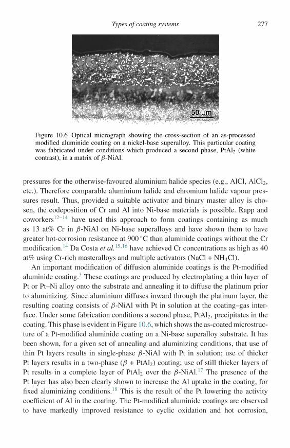
Types of coating systems 277
Figure 10.6 Optical micrograph showing the cross-section of an as-processedmodified aluminide coating on a nickel-base superalloy. This particular coatingwas fabricated under conditions which produced a second phase, PtAl2 (whitecontrast), in a matrix of β-NiAl.
pressures for the otherwise-favoured aluminium halide species (e.g., AlCl, AlCl2,etc.). Therefore comparable aluminium halide and chromium halide vapour pres-sures result. Thus, provided a suitable activator and binary master alloy is cho-sen, the codeposition of Cr and Al into Ni-base materials is possible. Rapp andcoworkers12–14 have used this approach to form coatings containing as muchas 13 at% Cr in β-NiAl on Ni-base superalloys and have shown them to havegreater hot-corrosion resistance at 900 ◦C than aluminide coatings without the Crmodification.14 Da Costa et al.15,16 have achieved Cr concentrations as high as 40at% using Cr-rich masteralloys and multiple activators (NaCl + NH4Cl).
An important modification of diffusion aluminide coatings is the Pt-modifiedaluminide coating.3 These coatings are produced by electroplating a thin layer ofPt or Pt–Ni alloy onto the substrate and annealing it to diffuse the platinum priorto aluminizing. Since aluminium diffuses inward through the platinum layer, theresulting coating consists of β-NiAl with Pt in solution at the coating–gas inter-face. Under some fabrication conditions a second phase, PtAl2, precipitates in thecoating. This phase is evident in Figure 10.6, which shows the as-coated microstruc-ture of a Pt-modified aluminide coating on a Ni-base superalloy substrate. It hasbeen shown, for a given set of annealing and aluminizing conditions, that use ofthin Pt layers results in single-phase β-NiAl with Pt in solution; use of thickerPt layers results in a two-phase (β + PtAl2) coating; use of still thicker layers ofPt results in a complete layer of PtAl2 over the β-NiAl.17 The presence of thePt layer has also been clearly shown to increase the Al uptake in the coating, forfixed aluminizing conditions.18 This is the result of the Pt lowering the activitycoefficient of Al in the coating. The Pt-modified aluminide coatings are observedto have markedly improved resistance to cyclic oxidation and hot corrosion,
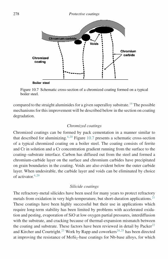
278 Protective coatings
Figure 10.7 Schematic cross-section of a chromized coating formed on a typicalboiler steel.
compared to the straight aluminides for a given superalloy substrate.19 The possiblemechanisms for this improvement will be described below in the section on coatingdegradation.
Chromized coatings
Chromized coatings can be formed by pack cementation in a manner similar tothat described for aluminizing.4,20 Figure 10.7 presents a schematic cross-sectionof a typical chromized coating on a boiler steel. The coating consists of ferriteand Cr in solution and a Cr concentration gradient running from the surface to thecoating–substrate interface. Carbon has diffused out from the steel and formed achromium-carbide layer on the surface and chromium carbides have precipitatedon grain boundaries in the coating. Voids are also evident below the outer carbidelayer. When undesirable, the carbide layer and voids can be eliminated by choiceof activator.4,20
Silicide coatings
The refractory-metal silicides have been used for many years to protect refractorymetals from oxidation in very high-temperature, but short-duration applications.21
These coatings have been highly successful but their use in applications whichrequire long-term stability has been limited by problems with accelerated oxida-tion and pesting, evaporation of SiO at low oxygen partial pressures, interdiffusionwith the substrate, and cracking because of thermal-expansion mismatch betweenthe coating and substrate. These factors have been reviewed in detail by Packer22
and Kircher and Courtright.23 Work by Rapp and coworkers24,25 has been directedat improving the resistance of MoSi2-base coatings for Nb-base alloys, for which
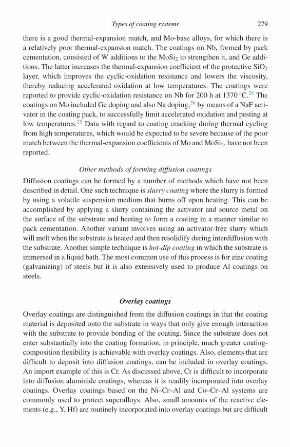
Types of coating systems 279
there is a good thermal-expansion match, and Mo-base alloys, for which there isa relatively poor thermal-expansion match. The coatings on Nb, formed by packcementation, consisted of W additions to the MoSi2 to strengthen it, and Ge addi-tions. The latter increases the thermal-expansion coefficient of the protective SiO2
layer, which improves the cyclic-oxidation resistance and lowers the viscosity,thereby reducing accelerated oxidation at low temperatures. The coatings werereported to provide cyclic-oxidation resistance on Nb for 200 h at 1370 ◦C.24 Thecoatings on Mo included Ge doping and also Na doping,26 by means of a NaF acti-vator in the coating pack, to successfully limit accelerated oxidation and pesting atlow temperatures.25 Data with regard to coating cracking during thermal cyclingfrom high temperatures, which would be expected to be severe because of the poormatch between the thermal-expansion coefficients of Mo and MoSi2, have not beenreported.
Other methods of forming diffusion coatings
Diffusion coatings can be formed by a number of methods which have not beendescribed in detail. One such technique is slurry coating where the slurry is formedby using a volatile suspension medium that burns off upon heating. This can beaccomplished by applying a slurry containing the activator and source metal onthe surface of the substrate and heating to form a coating in a manner similar topack cementation. Another variant involves using an activator-free slurry whichwill melt when the substrate is heated and then resolidify during interdiffusion withthe substrate. Another simple technique is hot-dip coating in which the substrate isimmersed in a liquid bath. The most common use of this process is for zinc coating(galvanizing) of steels but it is also extensively used to produce Al coatings onsteels.
Overlay coatings
Overlay coatings are distinguished from the diffusion coatings in that the coatingmaterial is deposited onto the substrate in ways that only give enough interactionwith the substrate to provide bonding of the coating. Since the substrate does notenter substantially into the coating formation, in principle, much greater coating-composition flexibility is achievable with overlay coatings. Also, elements that aredifficult to deposit into diffusion coatings, can be included in overlay coatings.An import example of this is Cr. As discussed above, Cr is difficult to incorporateinto diffusion aluminide coatings, whereas it is readily incorporated into overlaycoatings. Overlay coatings based on the Ni–Cr–Al and Co–Cr–Al systems arecommonly used to protect superalloys. Also, small amounts of the reactive ele-ments (e.g., Y, Hf) are routinely incorporated into overlay coatings but are difficult
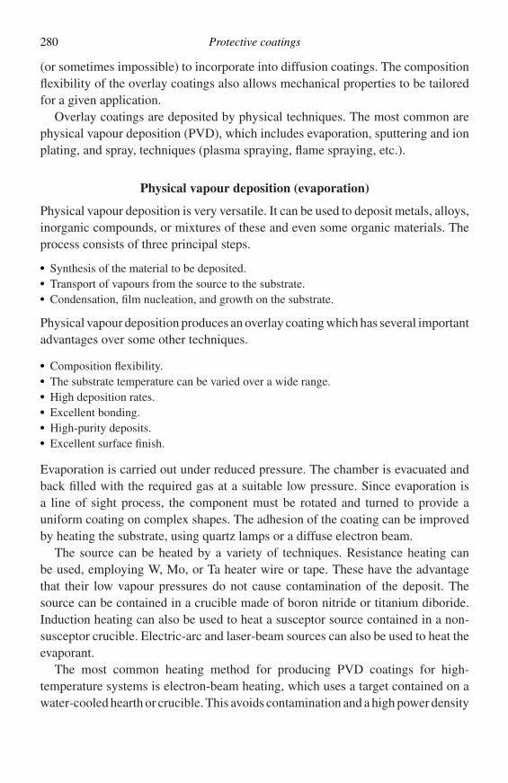
280 Protective coatings
(or sometimes impossible) to incorporate into diffusion coatings. The compositionflexibility of the overlay coatings also allows mechanical properties to be tailoredfor a given application.
Overlay coatings are deposited by physical techniques. The most common arephysical vapour deposition (PVD), which includes evaporation, sputtering and ionplating, and spray, techniques (plasma spraying, flame spraying, etc.).
Physical vapour deposition (evaporation)
Physical vapour deposition is very versatile. It can be used to deposit metals, alloys,inorganic compounds, or mixtures of these and even some organic materials. Theprocess consists of three principal steps.
� Synthesis of the material to be deposited.� Transport of vapours from the source to the substrate.� Condensation, film nucleation, and growth on the substrate.
Physical vapour deposition produces an overlay coating which has several importantadvantages over some other techniques.
� Composition flexibility.� The substrate temperature can be varied over a wide range.� High deposition rates.� Excellent bonding.� High-purity deposits.� Excellent surface finish.
Evaporation is carried out under reduced pressure. The chamber is evacuated andback filled with the required gas at a suitable low pressure. Since evaporation isa line of sight process, the component must be rotated and turned to provide auniform coating on complex shapes. The adhesion of the coating can be improvedby heating the substrate, using quartz lamps or a diffuse electron beam.
The source can be heated by a variety of techniques. Resistance heating canbe used, employing W, Mo, or Ta heater wire or tape. These have the advantagethat their low vapour pressures do not cause contamination of the deposit. Thesource can be contained in a crucible made of boron nitride or titanium diboride.Induction heating can also be used to heat a susceptor source contained in a non-susceptor crucible. Electric-arc and laser-beam sources can also be used to heat theevaporant.
The most common heating method for producing PVD coatings for high-temperature systems is electron-beam heating, which uses a target contained on awater-cooled hearth or crucible. This avoids contamination and a high power density
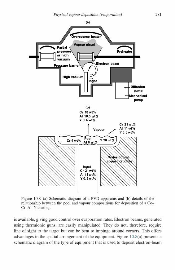
Physical vapour deposition (evaporation) 281
Figure 10.8 (a) Schematic diagram of a PVD apparatus and (b) details of therelationship between the pool and vapour compositions for deposition of a Co–Cr–Al–Y coating.
is available, giving good control over evaporation rates. Electron beams, generatedusing thermionic guns, are easily manipulated. They do not, therefore, requireline of sight to the target but can be bent to impinge around corners. This offersadvantages in the spatial arrangement of the equipment. Figure 10.8(a) presents aschematic diagram of the type of equipment that is used to deposit electron-beam
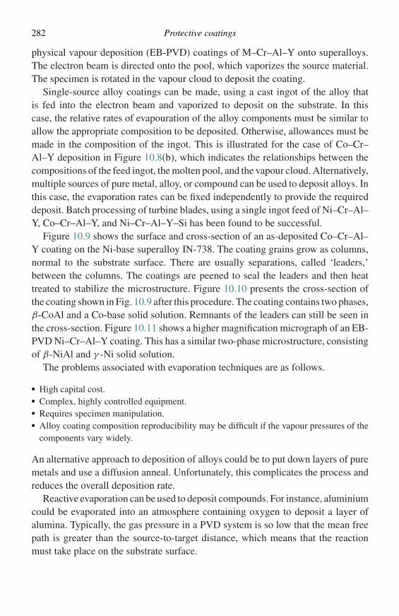
282 Protective coatings
physical vapour deposition (EB-PVD) coatings of M–Cr–Al–Y onto superalloys.The electron beam is directed onto the pool, which vaporizes the source material.The specimen is rotated in the vapour cloud to deposit the coating.
Single-source alloy coatings can be made, using a cast ingot of the alloy thatis fed into the electron beam and vaporized to deposit on the substrate. In thiscase, the relative rates of evapouration of the alloy components must be similar toallow the appropriate composition to be deposited. Otherwise, allowances must bemade in the composition of the ingot. This is illustrated for the case of Co–Cr–Al–Y deposition in Figure 10.8(b), which indicates the relationships between thecompositions of the feed ingot, the molten pool, and the vapour cloud. Alternatively,multiple sources of pure metal, alloy, or compound can be used to deposit alloys. Inthis case, the evaporation rates can be fixed independently to provide the requireddeposit. Batch processing of turbine blades, using a single ingot feed of Ni–Cr–Al–Y, Co–Cr–Al–Y, and Ni–Cr–Al–Y–Si has been found to be successful.
Figure 10.9 shows the surface and cross-section of an as-deposited Co–Cr–Al–Y coating on the Ni-base superalloy IN-738. The coating grains grow as columns,normal to the substrate surface. There are usually separations, called ‘leaders,’between the columns. The coatings are peened to seal the leaders and then heattreated to stabilize the microstructure. Figure 10.10 presents the cross-section ofthe coating shown in Fig. 10.9 after this procedure. The coating contains two phases,β-CoAl and a Co-base solid solution. Remnants of the leaders can still be seen inthe cross-section. Figure 10.11 shows a higher magnification micrograph of an EB-PVD Ni–Cr–Al–Y coating. This has a similar two-phase microstructure, consistingof β-NiAl and γ -Ni solid solution.
The problems associated with evaporation techniques are as follows.
� High capital cost.� Complex, highly controlled equipment.� Requires specimen manipulation.� Alloy coating composition reproducibility may be difficult if the vapour pressures of the
components vary widely.
An alternative approach to deposition of alloys could be to put down layers of puremetals and use a diffusion anneal. Unfortunately, this complicates the process andreduces the overall deposition rate.
Reactive evaporation can be used to deposit compounds. For instance, aluminiumcould be evaporated into an atmosphere containing oxygen to deposit a layer ofalumina. Typically, the gas pressure in a PVD system is so low that the mean freepath is greater than the source-to-target distance, which means that the reactionmust take place on the substrate surface.
Physical vapour deposition (evaporation) 283
(a)
20 µm
35 µm
(b)
Figure 10.9 (a) Scanning electron micrographs showing the surface and (b) cross-section of an EB-PVD Co–Cr–Al–Y overlay coating deposited on IN-738.
Plasma spray processes
The plasma spray technique has been used for about 30 years.27 Figure 10.12shows a simple schematic diagram of a plasma torch. Basically, a powder is fedinto the plasma, which is used as a heater, and the molten product is sprayed ontothe substrate to form just about any thickness. The coatings tend to be porous and ofpoor adhesion. The adhesion can be improved by increased surface roughness of thesubstrate, which can be produced by grit blasting. An interlayer bond coat of Ni–Al
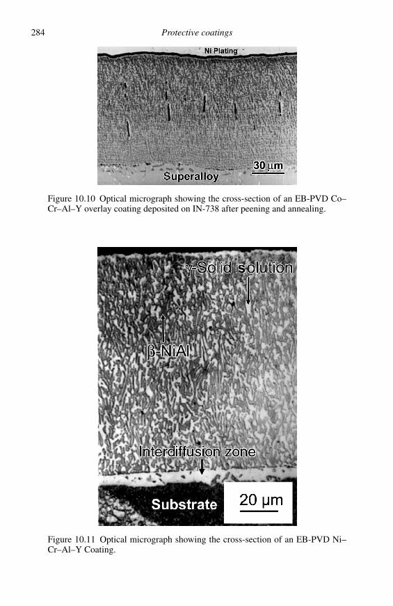
284 Protective coatings
Figure 10.10 Optical micrograph showing the cross-section of an EB-PVD Co–Cr–Al–Y overlay coating deposited on IN-738 after peening and annealing.
Figure 10.11 Optical micrograph showing the cross-section of an EB-PVD Ni–Cr–Al–Y Coating.
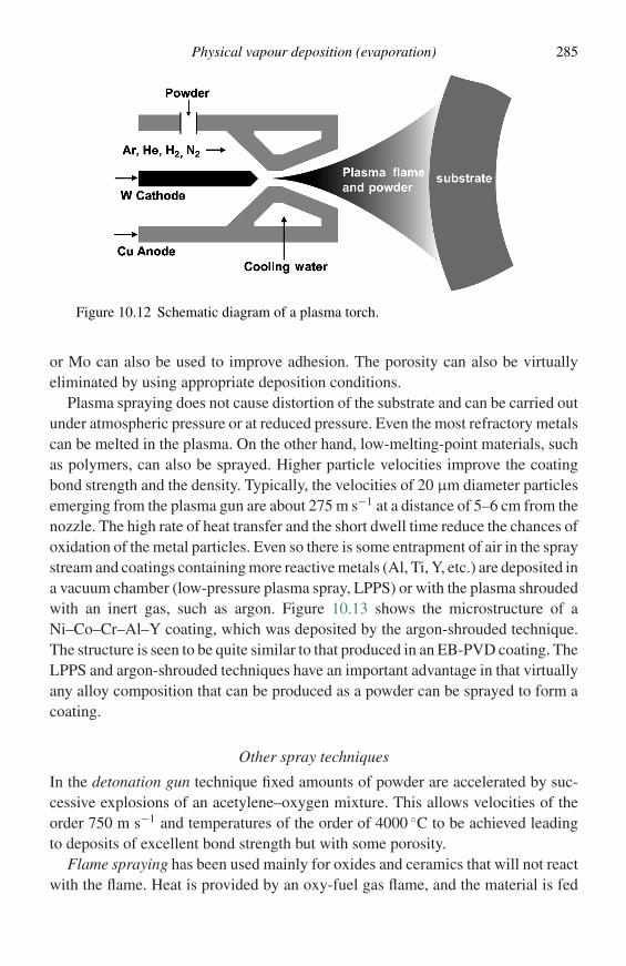
Physical vapour deposition (evaporation) 285
Figure 10.12 Schematic diagram of a plasma torch.
or Mo can also be used to improve adhesion. The porosity can also be virtuallyeliminated by using appropriate deposition conditions.
Plasma spraying does not cause distortion of the substrate and can be carried outunder atmospheric pressure or at reduced pressure. Even the most refractory metalscan be melted in the plasma. On the other hand, low-melting-point materials, suchas polymers, can also be sprayed. Higher particle velocities improve the coatingbond strength and the density. Typically, the velocities of 20 µm diameter particlesemerging from the plasma gun are about 275 m s−1 at a distance of 5–6 cm from thenozzle. The high rate of heat transfer and the short dwell time reduce the chances ofoxidation of the metal particles. Even so there is some entrapment of air in the spraystream and coatings containing more reactive metals (Al, Ti, Y, etc.) are deposited ina vacuum chamber (low-pressure plasma spray, LPPS) or with the plasma shroudedwith an inert gas, such as argon. Figure 10.13 shows the microstructure of aNi–Co–Cr–Al–Y coating, which was deposited by the argon-shrouded technique.The structure is seen to be quite similar to that produced in an EB-PVD coating. TheLPPS and argon-shrouded techniques have an important advantage in that virtuallyany alloy composition that can be produced as a powder can be sprayed to form acoating.
Other spray techniques
In the detonation gun technique fixed amounts of powder are accelerated by suc-cessive explosions of an acetylene–oxygen mixture. This allows velocities of theorder 750 m s−1 and temperatures of the order of 4000 ◦C to be achieved leadingto deposits of excellent bond strength but with some porosity.
Flame spraying has been used mainly for oxides and ceramics that will not reactwith the flame. Heat is provided by an oxy-fuel gas flame, and the material is fed
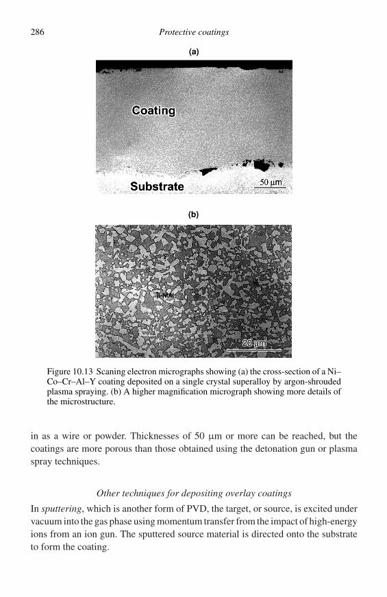
286 Protective coatings
(a)
(b)
Figure 10.13 Scaning electron micrographs showing (a) the cross-section of a Ni–Co–Cr–Al–Y coating deposited on a single crystal superalloy by argon-shroudedplasma spraying. (b) A higher magnification micrograph showing more details ofthe microstructure.
in as a wire or powder. Thicknesses of 50 µm or more can be reached, but thecoatings are more porous than those obtained using the detonation gun or plasmaspray techniques.
Other techniques for depositing overlay coatings
In sputtering, which is another form of PVD, the target, or source, is excited undervacuum into the gas phase using momentum transfer from the impact of high-energyions from an ion gun. The sputtered source material is directed onto the substrateto form the coating.
Physical vapour deposition (evaporation) 287
Cladding is perhaps the oldest form of coating. This consists of simply coveringa substrate with a protective surface layer. This is generally done mechanicallyusing roll bonding, coextrusion, or explosive cladding. Coextrusion has been usedfor applications in the electricity industry where the strength of low-grade, butinexpensive, steel tubes is supplemented with the oxidation resistance of materialssuch as stainless steel or IN-671 (50 wt% Ni–50 wt% Cr).
Thermal-barrier coatings
Thermal-barrier coatings (TBCs) are ceramic coatings which are applied to com-ponents for the purpose of insulation rather than oxidation protection. The use of aninsulating coating coupled with internal air cooling of the component, lowers thesurface temperature of the component with a corresponding decrease in the creepand oxidation rates of the component. The use of TBCs has resulted in a significantimprovement in the efficiency of gas turbines.28–30
The earliest TBCs were frit enamels which were applied to aircraft engine com-ponents in the 1950s.28 The first ceramic TBCs were applied by flame sprayingand, subsequently, by plasma spraying. The ceramic materials were alumina andzirconia (MgO- or CaO-stabilized), generally applied directly to the componentsurface. The effectiveness of these coatings was limited by the relatively highthermal conductivity of alumina and problems with destabilization of the zirconia-base materials.28 Important developments included the introduction of Ni–Cr–Al–Y bond coats and plasma-sprayed Y2O3-stabilized zirconia topcoats in the mid1970s and the development of EB-PVD to deposit the topcoat in the early 1980s.28
Plasma-sprayed TBCs have been used for many years on combustion liners but, withadvanced TBCs, vanes, and even the leading edges of blades, can now be coated.The use of TBCs can achieve temperature differentials across the coating of as muchas 175 ◦C.31
Typical systems, shown schematically in Figure 10.14, consist of a nickel-basesuperalloy substrate coated with M–Cr–Al–Y (M = Ni, Co) or a diffusion aluminidebond coat, which forms an alumina layer (thermally-grown oxide, TGO). Onto thisis deposited a yttria-stabilized zirconia (YSZ) TBC. The TBC can be deposited byair plasma spraying (APS), or EB-PVD. The EB-PVD coatings are used for themost demanding applications, such as the leading edges of airfoils. Figure 10.15presents cross-section micrographs of typical APS and EB-PVD TBCs. The APScoating consists of layers of splats with clearly visible porosity and is microcracked.This microcracking is necessary for strain tolerance. The EB-PVD coating consistsof columnar grains, which are separated by channels similar to the leaders seen inFigure 10.9 for a metallic overlay coating. These channels are responsible for theEB-PVD TBCs having a high strain tolerance.
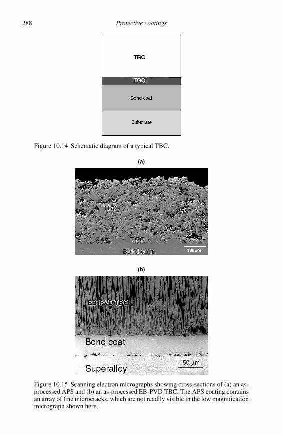
288 Protective coatings
Figure 10.14 Schematic diagram of a typical TBC.
(a)
(b)
Figure 10.15 Scanning electron micrographs showing cross-sections of (a) an as-processed APS and (b) an as-processed EB-PVD TBC. The APS coating containsan array of fine microcracks, which are not readily visible in the low magnificationmicrograph shown here.
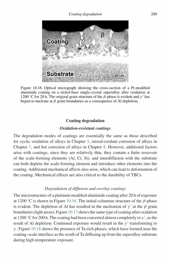
Coating degradation 289
Figure 10.16 Optical micrograph showing the cross-section of a Pt-modifiedaluminide coating on a nickel-base single-crystal superalloy after oxidation at1200 ◦C for 20 h. The original grain structure of the β-phase is evident and γ ′ hasbegun to nucleate at β grain boundaries as a consequence of Al depletion.
Coating degradation
Oxidation-resistant coatings
The degradation modes of coatings are essentially the same as those describedfor cyclic oxidation of alloys in Chapter 5, mixed-oxidant corrosion of alloys inChapter 7, and hot corrosion of alloys in Chapter 8. However, additional factorsarise with coatings; since they are relatively thin, they contain a finite reservoirof the scale-forming elements (Al, Cr, Si), and interdiffusion with the substratecan both deplete the scale-forming element and introduce other elements into thecoating. Additional mechanical affects also arise, which can lead to deformation ofthe coating. Mechanical effects are also critical to the durability of TBCs.
Degradation of diffusion and overlay coatings
The microstructure of a platinum modified aluminide coating after 20 h of exposureat 1200 ◦C is shown in Figure 10.16. The initial columnar structure of the β-phaseis evident. The depletion of Al has resulted in the nucleation of γ ′ at the β grainboundaries (light areas). Figure 10.17 shows the same type of coating after oxidationat 1200 ◦C for 200 h. The coating had been converted almost completely to γ ′, as theresult of Al depletion. Continued exposure would result in the γ ′ transforming toγ . Figure 10.18 shows the presence of Ta-rich phases, which have formed near thecoating–scale interface as the result of Ta diffusing up from the superalloy substrateduring high-temperature exposure.
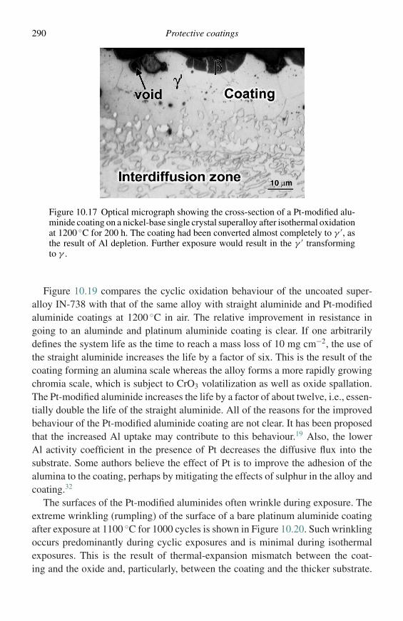
290 Protective coatings
Figure 10.17 Optical micrograph showing the cross-section of a Pt-modified alu-minide coating on a nickel-base single crystal superalloy after isothermal oxidationat 1200 ◦C for 200 h. The coating had been converted almost completely to γ ′, asthe result of Al depletion. Further exposure would result in the γ ′ transformingto γ .
Figure 10.19 compares the cyclic oxidation behaviour of the uncoated super-alloy IN-738 with that of the same alloy with straight aluminide and Pt-modifiedaluminide coatings at 1200 ◦C in air. The relative improvement in resistance ingoing to an aluminde and platinum aluminide coating is clear. If one arbitrarilydefines the system life as the time to reach a mass loss of 10 mg cm−2, the use ofthe straight aluminide increases the life by a factor of six. This is the result of thecoating forming an alumina scale whereas the alloy forms a more rapidly growingchromia scale, which is subject to CrO3 volatilization as well as oxide spallation.The Pt-modified aluminide increases the life by a factor of about twelve, i.e., essen-tially double the life of the straight aluminide. All of the reasons for the improvedbehaviour of the Pt-modified aluminide coating are not clear. It has been proposedthat the increased Al uptake may contribute to this behaviour.19 Also, the lowerAl activity coefficient in the presence of Pt decreases the diffusive flux into thesubstrate. Some authors believe the effect of Pt is to improve the adhesion of thealumina to the coating, perhaps by mitigating the effects of sulphur in the alloy andcoating.32
The surfaces of the Pt-modified aluminides often wrinkle during exposure. Theextreme wrinkling (rumpling) of the surface of a bare platinum aluminide coatingafter exposure at 1100 ◦C for 1000 cycles is shown in Figure 10.20. Such wrinklingoccurs predominantly during cyclic exposures and is minimal during isothermalexposures. This is the result of thermal-expansion mismatch between the coat-ing and the oxide and, particularly, between the coating and the thicker substrate.
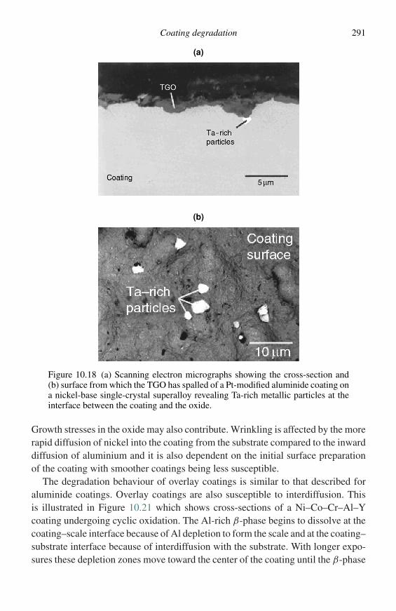
Coating degradation 291
(a)
(b)
Figure 10.18 (a) Scanning electron micrographs showing the cross-section and(b) surface from which the TGO has spalled of a Pt-modified aluminide coating ona nickel-base single-crystal superalloy revealing Ta-rich metallic particles at theinterface between the coating and the oxide.
Growth stresses in the oxide may also contribute. Wrinkling is affected by the morerapid diffusion of nickel into the coating from the substrate compared to the inwarddiffusion of aluminium and it is also dependent on the initial surface preparationof the coating with smoother coatings being less susceptible.
The degradation behaviour of overlay coatings is similar to that described foraluminide coatings. Overlay coatings are also susceptible to interdiffusion. Thisis illustrated in Figure 10.21 which shows cross-sections of a Ni–Co–Cr–Al–Ycoating undergoing cyclic oxidation. The Al-rich β-phase begins to dissolve at thecoating–scale interface because of Al depletion to form the scale and at the coating–substrate interface because of interdiffusion with the substrate. With longer expo-sures these depletion zones move toward the center of the coating until the β-phase
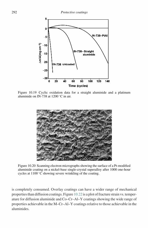
292 Protective coatings
Figure 10.19 Cyclic oxidation data for a straight aluminide and a platinumaluminide on IN-738 at 1200 ◦C in air.
Figure 10.20 Scanning electron micrographs showing the surface of a Pt-modifiedaluminide coating on a nickel-base single-crystal superalloy after 1000 one-hourcycles at 1100 ◦C showing severe wrinkling of the coating.
is completely consumed. Overlay coatings can have a wider range of mechanicalproperties than diffusion coatings. Figure 10.22 is a plot of fracture strain vs. temper-ature for diffusion aluminide and Co–Cr–Al–Y coatings showing the wide range ofproperties achievable in the M–Cr–Al–Y coatings relative to those achievable in thealuminides.
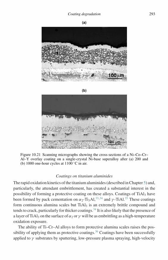
Coating degradation 293
(a)
(b)
Figure 10.21 Scanning micrographs showing the cross-sections of a Ni–Co–Cr–Al–Y overlay coating on a single-crystal Ni-base superalloy after (a) 200 and(b) 1000 one-hour cycles at 1100 ◦C in air.
Coatings on titanium aluminides
The rapid oxidation kinetics of the titanium aluminides (described in Chapter 5) and,particularly, the attendant embrittlement, has created a substantial interest in thepossibility of forming a protective coating on these alloys. Coatings of TiAl3 havebeen formed by pack cementation on α2-Ti3Al,33,34 and γ -TiAl.35 These coatingsform continuous alumina scales but TiAl3 is an extremely brittle compound andtends to crack, particularly for thicker coatings.34 It is also likely that the presence ofa layer of TiAl3 on the surface of α2 or γ will be as embrittling as a high-temperatureoxidation exposure.
The ability of Ti–Cr–Al alloys to form protective alumina scales raises the pos-sibility of applying them as protective coatings.36 Coatings have been successfullyapplied to γ substrates by sputtering, low-pressure plasma spraying, high-velocity
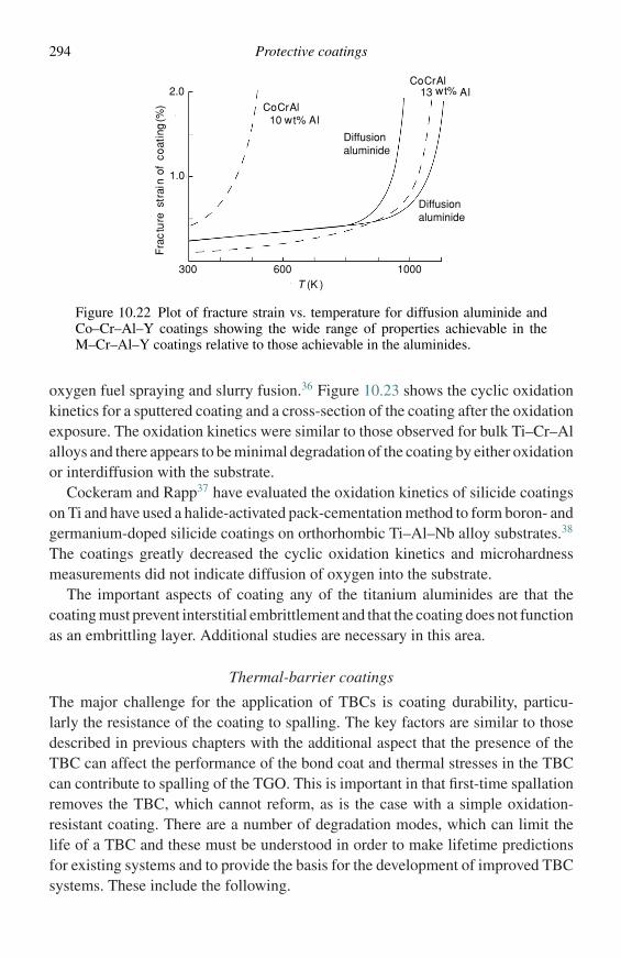
294 Protective coatings
1000600300
Diffusionaluminide
Diffusionaluminide
CoCrAl10 wt% Al
Fra
ctu
re s
trai
n of
co
atin
g (%
)
1.0
2.0 13 wt% Al
T (K )
CoCrAl
Figure 10.22 Plot of fracture strain vs. temperature for diffusion aluminide andCo–Cr–Al–Y coatings showing the wide range of properties achievable in theM–Cr–Al–Y coatings relative to those achievable in the aluminides.
oxygen fuel spraying and slurry fusion.36 Figure 10.23 shows the cyclic oxidationkinetics for a sputtered coating and a cross-section of the coating after the oxidationexposure. The oxidation kinetics were similar to those observed for bulk Ti–Cr–Alalloys and there appears to be minimal degradation of the coating by either oxidationor interdiffusion with the substrate.
Cockeram and Rapp37 have evaluated the oxidation kinetics of silicide coatingson Ti and have used a halide-activated pack-cementation method to form boron- andgermanium-doped silicide coatings on orthorhombic Ti–Al–Nb alloy substrates.38
The coatings greatly decreased the cyclic oxidation kinetics and microhardnessmeasurements did not indicate diffusion of oxygen into the substrate.
The important aspects of coating any of the titanium aluminides are that thecoating must prevent interstitial embrittlement and that the coating does not functionas an embrittling layer. Additional studies are necessary in this area.
Thermal-barrier coatings
The major challenge for the application of TBCs is coating durability, particu-larly the resistance of the coating to spalling. The key factors are similar to thosedescribed in previous chapters with the additional aspect that the presence of theTBC can affect the performance of the bond coat and thermal stresses in the TBCcan contribute to spalling of the TGO. This is important in that first-time spallationremoves the TBC, which cannot reform, as is the case with a simple oxidation-resistant coating. There are a number of degradation modes, which can limit thelife of a TBC and these must be understood in order to make lifetime predictionsfor existing systems and to provide the basis for the development of improved TBCsystems. These include the following.
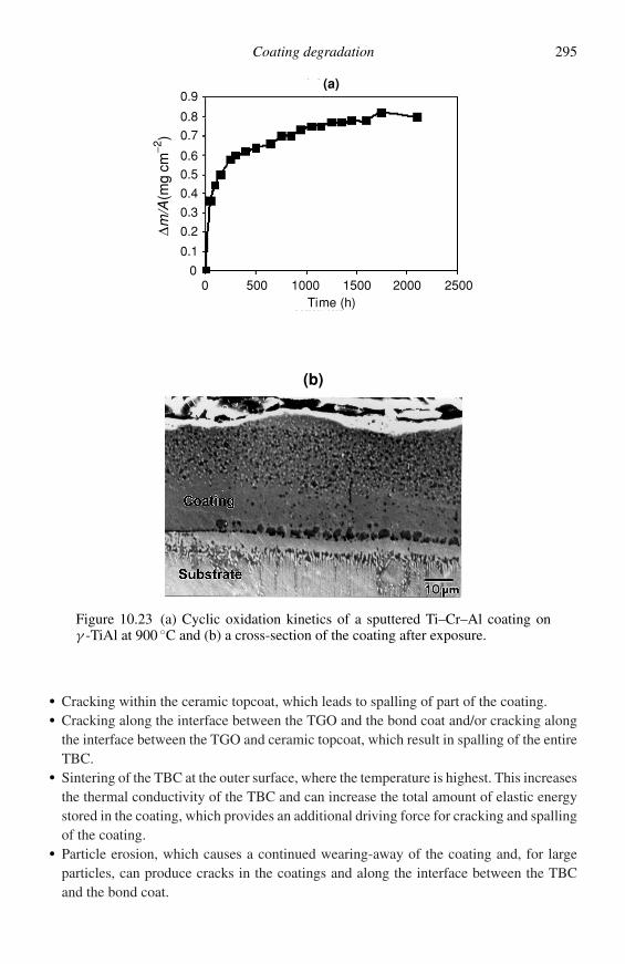
Coating degradation 295
0 500 1500 25001000 2000
(a)0.9
0.8
0.7
0.6
0.5
0.4
0.3
0.2
0.1
0
∆m/A
(mg
cm−2
)
Time (h)
(b)
Figure 10.23 (a) Cyclic oxidation kinetics of a sputtered Ti–Cr–Al coating onγ -TiAl at 900 ◦C and (b) a cross-section of the coating after exposure.
� Cracking within the ceramic topcoat, which leads to spalling of part of the coating.� Cracking along the interface between the TGO and the bond coat and/or cracking along
the interface between the TGO and ceramic topcoat, which result in spalling of the entireTBC.
� Sintering of the TBC at the outer surface, where the temperature is highest. This increasesthe thermal conductivity of the TBC and can increase the total amount of elastic energystored in the coating, which provides an additional driving force for cracking and spallingof the coating.
� Particle erosion, which causes a continued wearing-away of the coating and, for largeparticles, can produce cracks in the coatings and along the interface between the TBCand the bond coat.
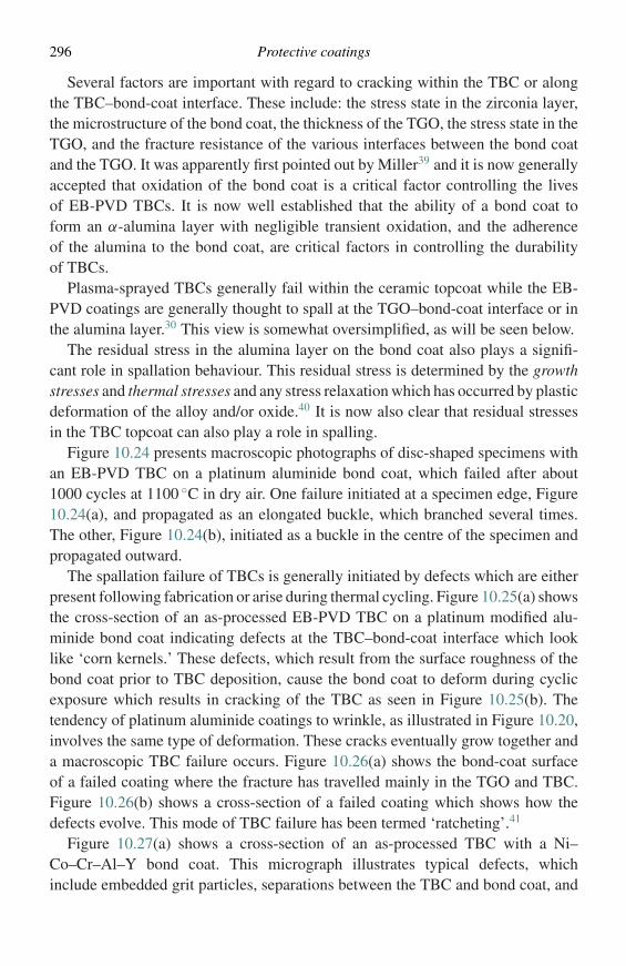
296 Protective coatings
Several factors are important with regard to cracking within the TBC or alongthe TBC–bond-coat interface. These include: the stress state in the zirconia layer,the microstructure of the bond coat, the thickness of the TGO, the stress state in theTGO, and the fracture resistance of the various interfaces between the bond coatand the TGO. It was apparently first pointed out by Miller39 and it is now generallyaccepted that oxidation of the bond coat is a critical factor controlling the livesof EB-PVD TBCs. It is now well established that the ability of a bond coat toform an α-alumina layer with negligible transient oxidation, and the adherenceof the alumina to the bond coat, are critical factors in controlling the durabilityof TBCs.
Plasma-sprayed TBCs generally fail within the ceramic topcoat while the EB-PVD coatings are generally thought to spall at the TGO–bond-coat interface or inthe alumina layer.30 This view is somewhat oversimplified, as will be seen below.
The residual stress in the alumina layer on the bond coat also plays a signifi-cant role in spallation behaviour. This residual stress is determined by the growthstresses and thermal stresses and any stress relaxation which has occurred by plasticdeformation of the alloy and/or oxide.40 It is now also clear that residual stressesin the TBC topcoat can also play a role in spalling.
Figure 10.24 presents macroscopic photographs of disc-shaped specimens withan EB-PVD TBC on a platinum aluminide bond coat, which failed after about1000 cycles at 1100 ◦C in dry air. One failure initiated at a specimen edge, Figure10.24(a), and propagated as an elongated buckle, which branched several times.The other, Figure 10.24(b), initiated as a buckle in the centre of the specimen andpropagated outward.
The spallation failure of TBCs is generally initiated by defects which are eitherpresent following fabrication or arise during thermal cycling. Figure 10.25(a) showsthe cross-section of an as-processed EB-PVD TBC on a platinum modified alu-minide bond coat indicating defects at the TBC–bond-coat interface which looklike ‘corn kernels.’ These defects, which result from the surface roughness of thebond coat prior to TBC deposition, cause the bond coat to deform during cyclicexposure which results in cracking of the TBC as seen in Figure 10.25(b). Thetendency of platinum aluminide coatings to wrinkle, as illustrated in Figure 10.20,involves the same type of deformation. These cracks eventually grow together anda macroscopic TBC failure occurs. Figure 10.26(a) shows the bond-coat surfaceof a failed coating where the fracture has travelled mainly in the TGO and TBC.Figure 10.26(b) shows a cross-section of a failed coating which shows how thedefects evolve. This mode of TBC failure has been termed ‘ratcheting’.41
Figure 10.27(a) shows a cross-section of an as-processed TBC with a Ni–Co–Cr–Al–Y bond coat. This micrograph illustrates typical defects, whichinclude embedded grit particles, separations between the TBC and bond coat, and
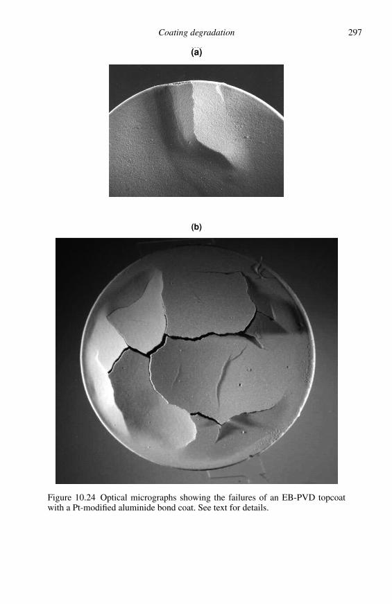
Coating degradation 297
(a)(a)
(b)
Figure 10.24 Optical micrographs showing the failures of an EB-PVD topcoatwith a Pt-modified aluminide bond coat. See text for details.
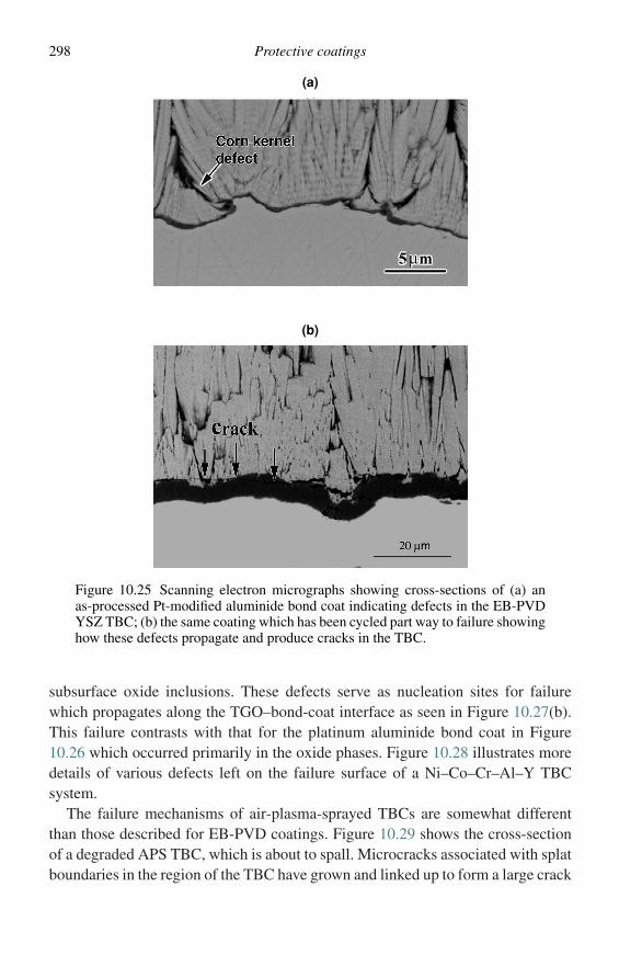
298 Protective coatings
(a)
(b)
Figure 10.25 Scanning electron micrographs showing cross-sections of (a) anas-processed Pt-modified aluminide bond coat indicating defects in the EB-PVDYSZ TBC; (b) the same coating which has been cycled part way to failure showinghow these defects propagate and produce cracks in the TBC.
subsurface oxide inclusions. These defects serve as nucleation sites for failurewhich propagates along the TGO–bond-coat interface as seen in Figure 10.27(b).This failure contrasts with that for the platinum aluminide bond coat in Figure10.26 which occurred primarily in the oxide phases. Figure 10.28 illustrates moredetails of various defects left on the failure surface of a Ni–Co–Cr–Al–Y TBCsystem.
The failure mechanisms of air-plasma-sprayed TBCs are somewhat differentthan those described for EB-PVD coatings. Figure 10.29 shows the cross-sectionof a degraded APS TBC, which is about to spall. Microcracks associated with splatboundaries in the region of the TBC have grown and linked up to form a large crack
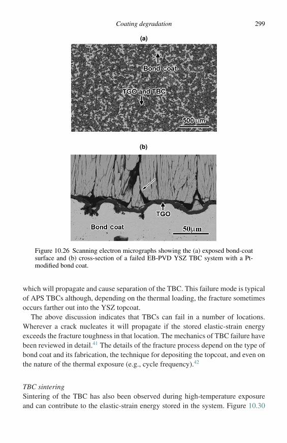
Coating degradation 299
(a)(a)
(b)
Figure 10.26 Scanning electron micrographs showing the (a) exposed bond-coatsurface and (b) cross-section of a failed EB-PVD YSZ TBC system with a Pt-modified bond coat.
which will propagate and cause separation of the TBC. This failure mode is typicalof APS TBCs although, depending on the thermal loading, the fracture sometimesoccurs farther out into the YSZ topcoat.
The above discussion indicates that TBCs can fail in a number of locations.Wherever a crack nucleates it will propagate if the stored elastic-strain energyexceeds the fracture toughness in that location. The mechanics of TBC failure havebeen reviewed in detail.41 The details of the fracture process depend on the type ofbond coat and its fabrication, the technique for depositing the topcoat, and even onthe nature of the thermal exposure (e.g., cycle frequency).42
TBC sinteringSintering of the TBC has also been observed during high-temperature exposureand can contribute to the elastic-strain energy stored in the system. Figure 10.30
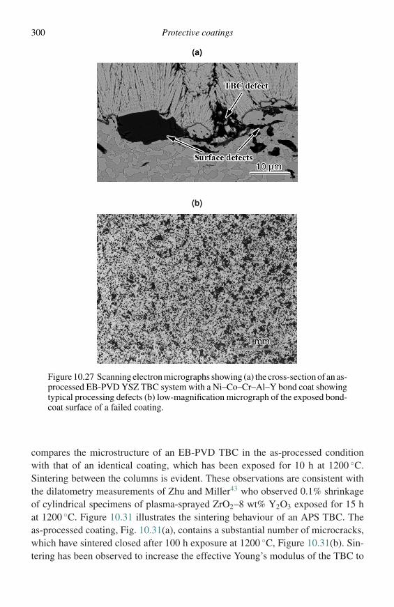
300 Protective coatings
(a)(a)
(b)
Figure 10.27 Scanning electron micrographs showing (a) the cross-section of an as-processed EB-PVD YSZ TBC system with a Ni–Co–Cr–Al–Y bond coat showingtypical processing defects (b) low-magnification micrograph of the exposed bond-coat surface of a failed coating.
compares the microstructure of an EB-PVD TBC in the as-processed conditionwith that of an identical coating, which has been exposed for 10 h at 1200 ◦C.Sintering between the columns is evident. These observations are consistent withthe dilatometry measurements of Zhu and Miller43 who observed 0.1% shrinkageof cylindrical specimens of plasma-sprayed ZrO2–8 wt% Y2O3 exposed for 15 hat 1200 ◦C. Figure 10.31 illustrates the sintering behaviour of an APS TBC. Theas-processed coating, Fig. 10.31(a), contains a substantial number of microcracks,which have sintered closed after 100 h exposure at 1200 ◦C, Figure 10.31(b). Sin-tering has been observed to increase the effective Young’s modulus of the TBC to
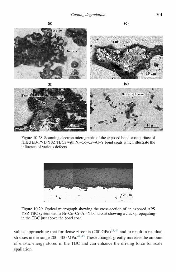
Coating degradation 301
(a)
(b)
(c)
µ
(d)
µ
Figure 10.28 Scanning electron micrographs of the exposed bond-coat surface offailed EB-PVD YSZ TBCs with Ni–Co–Cr–Al–Y bond coats which illustrate theinfluence of various defects.
125µm
Figure 10.29 Optical micrograph showing the cross-section of an exposed APSYSZ TBC system with a Ni–Co–Cr–Al–Y bond coat showing a crack propagatingin the TBC just above the bond coat.
values approaching that for dense zirconia (200 GPa)43,44 and to result in residualstresses in the range 200–400 MPa.44,45 These changes greatly increase the amountof elastic energy stored in the TBC and can enhance the driving force for scalespallation.
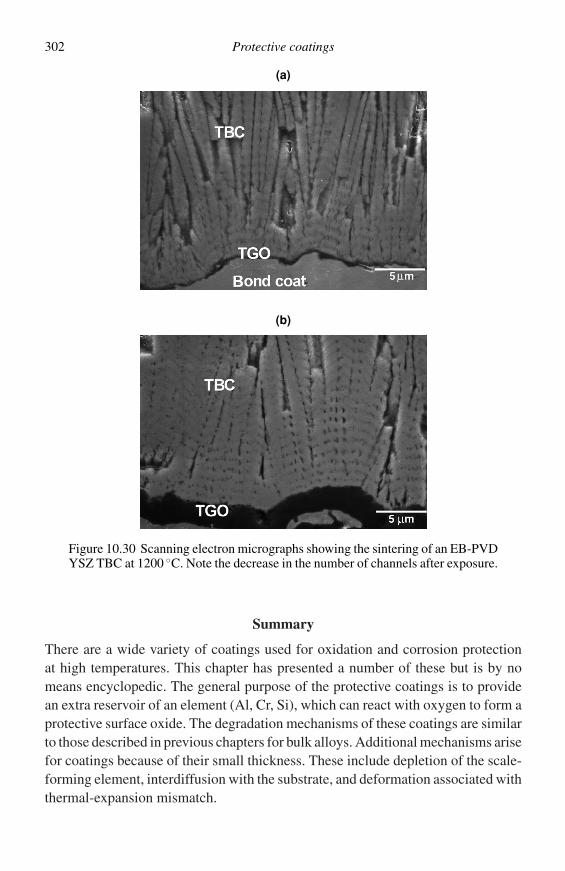
302 Protective coatings
(a)
(b)
Figure 10.30 Scanning electron micrographs showing the sintering of an EB-PVDYSZ TBC at 1200 ◦C. Note the decrease in the number of channels after exposure.
Summary
There are a wide variety of coatings used for oxidation and corrosion protectionat high temperatures. This chapter has presented a number of these but is by nomeans encyclopedic. The general purpose of the protective coatings is to providean extra reservoir of an element (Al, Cr, Si), which can react with oxygen to form aprotective surface oxide. The degradation mechanisms of these coatings are similarto those described in previous chapters for bulk alloys. Additional mechanisms arisefor coatings because of their small thickness. These include depletion of the scale-forming element, interdiffusion with the substrate, and deformation associated withthermal-expansion mismatch.
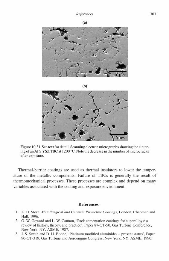
References 303
(a)
(b)
Figure 10.31 See text for detail. Scanning electron micrographs showing the sinter-ing of an APS YSZ TBC at 1200 ◦C. Note the decrease in the number of microcracksafter exposure.
Thermal-barrier coatings are used as thermal insulators to lower the temper-ature of the metallic components. Failure of TBCs is generally the result ofthermomechanical processes. These processes are complex and depend on manyvariables associated with the coating and exposure environment.
References
1. K. H. Stern, Metallurgical and Ceramic Protective Coatings, London, Chapman andHall, 1996.
2. G. W. Goward and L. W. Cannon, ‘Pack cementation coatings for superalloys: areview of history, theory, and practice’, Paper 87-GT-50, Gas Turbine Conference,New York, NY, ASME, 1987.
3. J. S. Smith and D. H. Boone, ‘Platinum modified aluminides – present status’, Paper90-GT-319, Gas Turbine and Aeroengine Congress, New York, NY, ASME, 1990.
304 Protective coatings
4. G. H. Meier, C. Cheng, R. A. Perkins, and W. Bakker, Surf. Coatings Tech., 39/40(1989), 53.
5. S. R. Levine and R. M. Caves, J. Electrochem Soc., 121 (1974), 1051.6. B. K. Gupta, A. K. Sarkhel, and L. L. Seigle, Thin Solid Films, 39 (1976), 313.7. S. Shankar and L. L. Seigle, Met. Trans., 9A (1978), 1476.8. B. K. Gupta and L. L. Seigle, Thin Solid Films, 73 (1980), 365.9. N. Kandasamy, L. L. Seigle, and F. J. Pennisi, Thin Solid Films, 84 (1981), 17.
10. G. W. Goward and D. H. Boone, Oxid. Met., 3 (1971), 475.11. S. C. Kung and R. A. Rapp, Oxid. Met., 32 (1989), 89.12. R. Bianco and R. A. Rapp, J. Electrochem. Soc., 140 (1993), 1181.13. R. Bianco and R. A. Rapp, in High Temperature Materials Chemistry-V, eds. W. B.
Johnson and R. A. Rapp, New York, NY, The Electrochemical Society, 1990, p. 211.14. R. Bianco, R. A. Rapp, and J. L. Smialek, J. Electrochem. Soc., 140 (1993), 1191.15. W. Da Costa, B. Gleeson, and D. J. Young, J. Electrochem. Soc., 141 (1994), 1464.16. W. Da Costa, B. Gleeson, and D. J. Young, J. Electrochem. Soc., 141 (1994), 2690.17. G. R. Krishna, D. K. Das, V. Singh, and S. V. Joshi, Mater. Sci. Eng., A251 (1998),
40.18. M. R. Jackson and J. R. Rairden, Met. Trans., 8A (1977), 1697.19. J. Schaeffer, G. M. Kim, G. H. Meier, and F. S. Pettit, ‘The effects of precious metals
on the oxidation and hot corrosion of coatings’. In The Role of Active Elements in theOxidation Behavior of High Temperature Metals and Alloys, ed. E. Lang,Amsterdam, Elsevier, 1989, p. 231.
20. G. H. Meier, C. Cheng, R. A. Perkins, and W. T. Bakker, Formation of chromiumdiffusion coatings on low alloy steels for use in coal conversion atmospheres. InMaterials For Coal Gasification, eds. W. T. Bakker, S. Dapkunas, and V. Hill, MetalsPark, OH, ASM International, 1988, p. 159.
21. H. Lavendel, R. A. Perkins, A. G. Elliot, and J. Ong, Investigation of modifiedsilicide coatings for refractory metal alloys with improved low pressure oxidationbehavior. Report on Air Force Contract, AFML-TR-65-344, Palo Alto, CA,Lockheed Palo Alto Research Laboratory, 1965.
22. C. M. Packer, in Oxidation of High-Temperature Intermetallics, eds. T. Grobstein andJ. Doychak, Warrendale, PA, The Mining, Metallurgy, and Materials Society, 1989,p. 235.
23. T. A. Kircher and E. L. Courtright, Mater. Sci. Eng., A155 (1992), 67.24. A. Mueller, G. Wang, R. A. Rapp, and E. L. Courtright, J. Electrochem. Soc., 139
(1992), 1266.25. B. V. Cockeram, G. Wang, and R. A. Rapp, Mater. Corr., 46 (1995), 207.26. B. V. Cockeram, G. Wang, and R. A. Rapp, Oxid. Met., 45 (1996), 77.27. R. C., Tucker, Jr., Thermal spray coatings. In Handbook of Thin Film Process
Technology, eds. S. I. Shah and D. Glocker, Bristol, IOP Publishing Ltd, 1996, p.A4.0:1.
28. R. A. Miller, Thermal barrier coatings for aircraft engines – history and directions.Proceedings of Thermal Barrier Coating Workshop, Cleveland, OH, March 27–29,1995, p. 17 (NASA CP 3812).
29. A. Maricocchi, A. Bartz, and D. Wortman, PVD TBC experience on GE aircraftengines. Proceedings of Thermal Barrier Coating Workshop, Cleveland, OH, March27–29, 1995, p. 79 (NASA CP 3312).
30. S. Bose and J. T. DeMasi-Marcin, Thermal barrier coating experience in gas turbineengines at Pratt & Whitney. Proceedings of Thermal Barrier Coating Workshop,Cleveland, OH, March 27–29, 1995, p. 63 (NASA CP 3312).
References 305
31. J. T. DeMasi-Marcin and D. K. Gupta, Surf. Coatings Tech., 68–69 (1994), 1.32. J. A. Haynes, Y. Zhang, W. Y. Lee, B. A. Pint, I. G. Wright, and K. M., Cooley,
Effects of platinum additions and sulfur impurities on the microstructure and scaleadhesion behavior of single-phase CVD aluminide bond coatings. In ElevatedTemperature Coatings, eds. J. M. Hampikian and N. B. Dahotre, Warrendale, PA,TMS, 1999, p. 51.
33. J. Subrahmanyam, J. Mater. Sci., 23 (1988), 1906.34. J. L. Smialek, M. A. Gedwill, and P. K. Brindley, Scripta met. mater., 24 (1990),
1291.35. H. Mabuchi, T. Asai, and Y. Nakayama, Scripta met., 23 (1989), 685.36. R. L. McCarron, J. C. Schaeffer, G. H. Meier, D. Berztiss, R. A. Perkins, and J.
Cullinan, Protective coatings for titanium aluminide intermetallics. In Titanium ’92,eds. F. H. Froes and I. L. Caplan, Warrendale, PA, TMS, 1993, p. 1,971.
37. B. V. Cockeram and R. A. Rapp, Met. Mater. Trans., 26A (1995), 777.38. B. V. Cockeram and R. A. Rapp, Boron-modified and germanium-doped silicide
diffusion coatings for Ti–Al–Nb, Nb–Ti–Al, Nb–Cr and Nb–base alloys. InProcessing and Design Issues in High Temperature Materials, eds. N. S. Stoloff andR. H. Jones, Warrendale, PA, Mining, Metallurgy and Meterials Society, 1996, p.391.
39. R. Miller, J. Amer. Ceram. Soc., 67 (1984), 517.40. M. J. Stiger, N. M. Yanar, M. G. Topping, F. S. Pettit, and G. H. Meier,
Z. Metallkunde, 90 (1999), 1069.41. A. G. Evans, D. R. Mumm, J. W. Hutchinson, G. H. Meier, and F. S. Pettit, Progr.
Mater. Sci., 46 (2001), 505.42. G. M. Kim, N. M. Yanar, E. N. Hewitt, F. S. Pettit, and G. H. Meier, Scripta Mater.,
46 (2002), 489.43. D. Zhu and R. A. Miller, Surf. Coatings Tech., 108–109 (1998), 114.44. C. A. Johnson, J. A. Ruud, R. Bruce, and D. Wortman, Surf. Coatings Tech., 108–109
(1998), 80.45. J. Thornton, D. Cookson, and E. Pescott, Surf. Coatings Tech., 120–121 (1999), 96.
11
Atmosphere control for the protection of metalsduring production processes
Introduction
The exposure of metals to gases at high temperatures during production processesmay be divided broadly under two headings.
(1) Reheating for subsequent working or shaping.(2) Reheating for final heat treatment, sometimes of finished components.
When reheating for subsequent working or shaping, the main concern is to heatthe components as quickly and economically as possible to the working temper-ature, within the metallurgical constraint of avoiding element redistribution andthermal cracking. In addition, it is usual to expose the metal directly to a burned-fuel atmosphere containing about 1% excess oxygen necessary to ensure completecombustion and, therefore, the most economic use of the fuel. Under these con-ditions, as there is little likelihood of operating a controlled-atmosphere policy,surface damage due to oxidation or scaling and, in the case of steels, decarburiza-tion, must be removed at a later stage in the process. Indeed, if the surface of thematerial to be reheated already has some undesirable features, it may be possibleto remove, or reduce, them by allowing some scaling to occur.
Alloys which are susceptible to surface deterioration during reheating may beprotected either by controlling the atmosphere composition to minimize, or avoid,surface deterioration or by applying a coating to protect the alloy from the atmos-phere.
Coatings are not an economic proposition in the treatment of large tonnageproduction in this way, but are applied to cause selective carburization, etc., duringsurface-hardening procedures. Alternatively, coating application is common duringservice (See Chapter 10) and is a fairly successful way to avoid short-term damageto the underlying alloy.
This chapter is concerned with the use of gaseous atmospheres to control sur-face reactions during reheating for working or heat treatment. The main application
306
Prevention or control of oxide-layer formation 307
of controlled atmospheres is in the area of heat treatment of finished, machined,components or of articles of complex shape, which cannot easily be treated subse-quently for the removal of surface damage. In this context, atmosphere control canbe considered under two headings: firstly, where the treatment is aimed simply toprevent surface reaction; and secondly, where it is designed to cause a particularsurface reaction to proceed such as carburizing or nitriding. We are concerned onlywith the former.
Prevention or control of oxide-layer formation
This is primarily a question of controlling the oxygen partial pressure of the atmos-phere to a value low enough to prevent oxidation, as described in Chapter 2. Verysimply, for a metal which undergoes oxidation according to the reaction shown inEquation (11.1),
M + 1
2O2 = MO; �Go
1, (11.1)
where MO is the lowest oxide of M, the oxygen partial pressure must be controlledso as not to exceed a value, (pO2)M−MO, Equation (11.2):
(pO2)M−MO = exp
(2�Go
1
RT
). (11.2)
Unfortunately (pO2)M−MO is a function of temperature and has lower values atlower temperatures. Thus, if an atmosphere is designed to be effective at high tem-peratures it may become oxidizing as the temperature is reduced during cooling. Asurface oxide layer may, therefore, form as the metal is cooled. Although the met-allurgical damage to the surface will be negligible, the surface may be discoloured,i.e., not bright. This condition can be overcome to some extent by rapid coolingor by changing the atmosphere to a lower oxygen partial pressure just before orduring cooling.
For alloys, it is clear that the most critical reaction must be considered whendeciding on the composition of the atmosphere to be used. For this purpose, theactivities of the alloy components must be known since, if the metal M in Equation(11.1) exists at an activity aM the corresponding equilibrium oxygen partial pressurewill be given by Equation (11.3):
(pO2)M−MO = 1
a2M
exp
(2�Go
1
RT
). (11.3)
If the metal activities in the alloy are not known, then, by assuming the solutionto be ideal, mole fractions may be used instead of activities to give a value of the
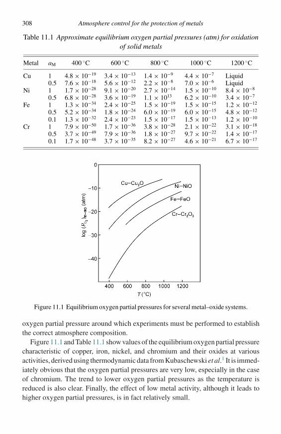
308 Atmosphere control for the protection of metals
Table 11.1 Approximate equilibrium oxygen partial pressures (atm) for oxidationof solid metals
Metal aM 400 ◦C 600 ◦C 800 ◦C 1000 ◦C 1200 ◦C
Cu 10.5
4.8 × 10⁻¹⁹
7.6 × 10−183.4 × 10⁻¹³
5.6 × 10−121.4 × 10⁻⁹
2.2 × 10−84.4 × 10−7
7.0 × 10⁻⁶LiquidLiquid
Ni 10.5
1.7 × 10⁻²⁸
6.8 × 10−289.1 × 10⁻²⁰
3.6 × 10−192.7 × 10⁻¹⁴
1.1 × 10131.5 × 10−10
6.2 × 10−108.4 × 10⁻⁸
3.4 × 10⁻⁷
Fe 10.50.1
1.3 × 10⁻³⁴
5.2 × 10⁻³⁴
1.3 × 10⁻³²
2.4 × 10⁻²⁵
1.8 × 10⁻²⁴
2.4 × 10⁻²³
1.5 × 10⁻¹⁹
6.0 × 10⁻¹⁹
1.5 × 10⁻¹⁷
1.5 × 10⁻¹⁵
6.0 × 10⁻¹⁵
1.5 × 10⁻¹³
1.2 × 10⁻¹²
4.8 × 10⁻¹²
1.2 × 10⁻¹⁰
Cr 10.50.1
7.9 × 10−50
3.7 × 10−49
1.7 × 10−48
1.7 × 10−36
7.9 × 10−36
3.7 × 10⁻³⁵
3.8 × 10⁻²⁸
1.8 × 10⁻²⁷
8.2 × 10⁻²⁷
2.1 × 10⁻²²
9.7 × 10⁻²²
4.6 × 10⁻²¹
3.1 × 10⁻¹⁸
1.4 × 10⁻¹⁷
6.7 × 10⁻¹⁷
O
Figure 11.1 Equilibrium oxygen partial pressures for several metal–oxide systems.
oxygen partial pressure around which experiments must be performed to establishthe correct atmosphere composition.
Figure 11.1 and Table 11.1 show values of the equilibrium oxygen partial pressurecharacteristic of copper, iron, nickel, and chromium and their oxides at variousactivities, derived using thermodynamic data from Kubaschewski et al.1 It is immed-iately obvious that the oxygen partial pressures are very low, especially in the caseof chromium. The trend to lower oxygen partial pressures as the temperature isreduced is also clear. Finally, the effect of low metal activity, although it leads tohigher oxygen partial pressures, is in fact relatively small.
Protective atmospheres in the laboratory 309
Provision of protective atmospheres in the laboratory
Vacuum
To carry out heat treatment in vacuum is the first, and perhaps the simplest, methodof avoiding surface oxide formation to be considered. If the vacuum is against air,as is usual, it is possible to reduce the oxygen partial pressure to values as low as10−10 or 10−11 atm. Comparing this with the values in Figure 11.1 it is seen that thisshould be effective for copper above 670 ◦C, nickel above 950 ◦C, and iron above1200 ◦C, but not at all for chromium. Due to the very low reaction rates, however,it is generally possible to extend these limits to lower temperatures depending onthe time of treatment.
With vacuum treatment there is always the possibility, especially at the highertemperatures, of the loss of volatile metals, such as manganese, from the surfaceregions of the component. For example, brass treated in this manner will undergoserious, if not total loss of zinc.
Even with modern techniques, vacua of the above levels can only be achieved inrelatively small chambers and the technique is largely restricted to laboratory use.
Gaseous atmospheres
Purified inert gases, mainly argon, can be used. However, due to the difficulty ofreducing the oxygen partial pressure below 10−6 atm, such atmospheres rely for theireffect largely on the reduced reaction rate at these reduced oxygen partial pressures.Inert atmospheres are also expensive to produce and are, therefore, largely restrictedto the laboratory.
Low oxygen partial pressures can be provided and, more importantly, controlledby using ‘redox’ gas mixtures. These mixtures consist of an oxidized and a reducedspecies, which equilibrate with oxygen, e.g., Equation (11.4),
CO (g) + 1
2O2 (g) = CO2 (g); �Go
4 = −282 200 + 86.7T J, (11.4)
from which pO2 or, more importantly, pCO2/pCO can be obtained:
pO2 =(
pCO2
pCO
)2
exp
(2�Go
4
RT
), (11.5a)
pCO2
pCO= p1/2
O2exp
(−�Go4
RT
). (11.5b)
Thus from Equation (11.5b) the ratio of carbon dioxide to carbon monoxide maybe calculated for any oxygen partial pressure and temperature.
In Figure 11.2 corresponding values of the ratio pCO2/pCO and pO2 are plottedfor the temperatures 400, 600, 800, 1000, and 1200 ◦C. The lines corresponding
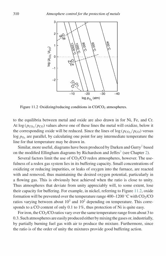
310 Atmosphere control for the protection of metals
−10 −20 −30 −40log pO2
(atm)
log
(pC
O2/p
CO
)
400°C
600°C
800°C
1000°C
12000°C
FeOFe
Cr2 O3Cr
NiONi
3
2
1
0
−1
−2
Figure 11.2 Oxidizing/reducing conditions in CO/CO2 atmospheres.
to the equilibria between metal and oxide are also drawn in for Ni, Fe, and Cr.At log (pCO2/pCO) values above one of these lines the metal will oxidize, below itthe corresponding oxide will be reduced. Since the lines of log (pCO2/pCO) versuslog pO2 are parallel, by calculating one point for any intermediate temperature theline for that temperature may be drawn in.
Similar, more useful, diagrams have been produced by Darken and Gurry2 basedon the modified Ellingham diagrams by Richardson and Jeffes3 (see Chapter 2).
Several factors limit the use of CO2/CO redox atmospheres, however. The use-fulness of a redox gas system lies in its buffering capacity. Small concentrations ofoxidizing or reducing impurities, or leaks of oxygen into the furnace, are reactedwith and removed, thus maintaining the desired oxygen potential, particularly ina flowing gas. This is obviously best achieved when the ratio is close to unity.Thus atmospheres that deviate from unity appreciably will, to some extent, losetheir capacity for buffering. For example, in nickel, referring to Figure 11.2, oxideformation will be prevented over the temperature range 400–1200 ◦C with CO2/COratios varying between about 103 and 102 depending on temperature. This corre-sponds to a CO content of only 0.1 to 1%, thus protection of Ni is quite easy.
For iron, the CO2/CO ratios vary over the same temperature range from about 3 to0.3. Such atmospheres are easily produced either by mixing the gases or, industrially,by partially burning fuel gas with air to produce the mixture. Furthermore, sincethe ratio is of the order of unity the mixtures provide good buffering action.
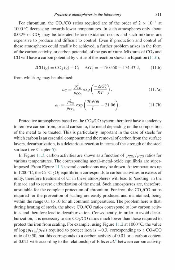
Protective atmospheres in the laboratory 311
For chromium, the CO2/CO ratios required are of the order of 2 × 10⁻⁴ at1000 ◦C decreasing towards lower temperatures. In such atmospheres only about0.02% of CO2 may be tolerated before oxidation occurs and such mixtures areexpensive to produce and difficult to control. Even if production and control ofthese atmospheres could readily be achieved, a further problem arises in the formof the carbon activity, or carbon potential, of the gas mixture. Mixtures of CO2 andCO will have a carbon potential by virtue of the reaction shown in Equation (11.6),
2CO (g) = CO2 (g) + C; �Go6 = −170 550 + 174.3T J, (11.6)
from which aC may be obtained:
aC = p2CO
pCO2
exp
(−�Go6
RT
), (11.7a)
aC = p2CO
pCO2
exp
(20 606
T− 21.06
). (11.7b)
Protective atmospheres based on the CO2/CO system therefore have a tendencyto remove carbon from, or add carbon to, the metal depending on the compositionof the metal to be treated. This is particularly important in the case of steels forwhich carbon is an essential component and the removal of carbon from the surfacelayers, decarburization, is a deleterious reaction in terms of the strength of the steelsurface (see Chapter 5).
In Figure 11.3, carbon activities are shown as a function of pCO2/pCO ratios forvarious temperatures. The corresponding metal–metal-oxide equilibria are super-imposed. From Figure 11.3 several conclusions may be drawn. At temperatures upto 1200 ◦C, the Cr–Cr2O3 equilibrium corresponds to carbon activities in excess ofunity, therefore treatment of Cr in these atmospheres will lead to ‘sooting’ in thefurnace and to severe carburization of the metal. Such atmospheres are, therefore,unsuitable for the complete protection of chromium. For iron, the CO2/CO ratiosrequired for the prevention of scaling are easily produced and maintained, beingwithin the range 0.1 to 10 for all common temperatures. The problem here is that,during heating of steels, the above CO2/CO ratios correspond to low carbon activ-ities and therefore lead to decarburization. Consequently, in order to avoid decar-burization, it is necessary to use CO2/CO ratios much lower than those required toprotect the iron from scaling. For example, using Figure 11.2 at 1000 ◦C, the valueof log (pCO2/pCO) required to protect iron is −0.3, corresponding to a CO2/COratio of 0.50, but this corresponds to a carbon activity of 0.01 or a carbon contentof 0.021 wt% according to the relationship of Ellis et al.4 between carbon activity,
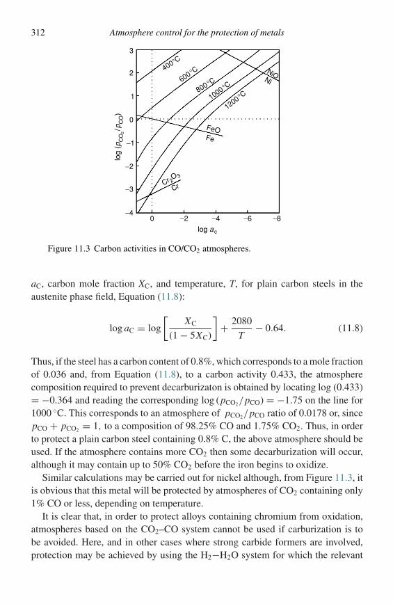
312 Atmosphere control for the protection of metals
log
(pC
O2/p
CO
)
Figure 11.3 Carbon activities in CO/CO2 atmospheres.
aC, carbon mole fraction XC, and temperature, T, for plain carbon steels in theaustenite phase field, Equation (11.8):
log aC = log
[XC
(1 − 5XC)
]+ 2080
T− 0.64. (11.8)
Thus, if the steel has a carbon content of 0.8%, which corresponds to a mole fractionof 0.036 and, from Equation (11.8), to a carbon activity 0.433, the atmospherecomposition required to prevent decarburizaton is obtained by locating log (0.433)= −0.364 and reading the corresponding log (pCO2/pCO) = −1.75 on the line for1000 ◦C. This corresponds to an atmosphere of pCO2/pCO ratio of 0.0178 or, sincepCO + pCO2 = 1, to a composition of 98.25% CO and 1.75% CO2. Thus, in orderto protect a plain carbon steel containing 0.8% C, the above atmosphere should beused. If the atmosphere contains more CO2 then some decarburization will occur,although it may contain up to 50% CO2 before the iron begins to oxidize.
Similar calculations may be carried out for nickel although, from Figure 11.3, itis obvious that this metal will be protected by atmospheres of CO2 containing only1% CO or less, depending on temperature.
It is clear that, in order to protect alloys containing chromium from oxidation,atmospheres based on the CO2–CO system cannot be used if carburization is tobe avoided. Here, and in other cases where strong carbide formers are involved,protection may be achieved by using the H2−H2O system for which the relevant
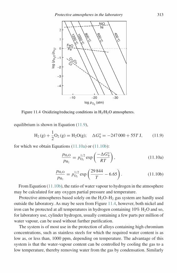
Protective atmospheres in the laboratory 313
Cr2 O3Cr
NiONi
400°C
600°C
800°C
1000°C
1200°C
FeOFe
log pO2 (atm)
log
(pH
2O/p
H2)
−10
−4
−3
−2
−1
0
1
2
−20 −30
Figure 11.4 Oxidizing/reducing conditions in H2/H2O atmospheres.
equilibrium is shown in Equation (11.9),
H2 (g) + 1
2O2 (g) = H2O(g); �Go
9 = −247 000 + 55T J, (11.9)
for which we obtain Equations (11.10a) or (11.10b):
pH2O
pH2
= p1/2O2
exp
(−�Go9
RT
), (11.10a)
pH2O
pH2
= p1/2O2
exp
(29 844
T− 6.65
). (11.10b)
From Equation (11.10b), the ratio of water vapour to hydrogen in the atmospheremay be calculated for any oxygen partial pressure and temperature.
Protective atmospheres based solely on the H2O–H2 gas system are hardly usedoutside the laboratory. As may be seen from Figure 11.4, however, both nickel andiron can be protected at all temperatures in hydrogen containing 10% H2O and so,for laboratory use, cylinder hydrogen, usually containing a few parts per million ofwater vapour, can be used without further purification.
The system is of most use in the protection of alloys containing high chromiumconcentrations, such as stainless steels for which the required water content is aslow as, or less than, 1000 ppm, depending on temperature. The advantage of thissystem is that the water-vapour content can be controlled by cooling the gas to alow temperature, thereby removing water from the gas by condensation. Similarly
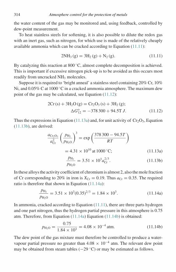
314 Atmosphere control for the protection of metals
the water content of the gas may be monitored and, using feedback, controlled bydew-point measurement.
To heat stainless steels for softening, it is also possible to dilute the redox gaswith an inert gas, such as nitrogen, for which use is made of the relatively cheaplyavailable ammonia which can be cracked according to Equation (11.11):
2NH3 (g) = 3H2 (g) + N2 (g). (11.11)
By catalyzing this reaction at 800 ◦C, almost complete decomposition is achieved.This is important if excessive nitrogen pick-up is to be avoided as this occurs mostreadily from uncracked NH3 molecules.
Suppose it is required to ‘bright anneal’ a stainless steel containing 20% Cr, 10%Ni, and 0.05% C at 1000 ◦C in a cracked ammonia atmosphere. The maximum dewpoint of the gas may be calculated, see Equation (11.12):
2Cr (s) + 3H2O (g) = Cr2O3 (s) + 3H2 (g);
�Go12 = −378 300 + 94.5T J. (11.12)
Thus the expressions in Equation (11.13a) and, for unit activity of Cr2O3, Equation(11.13b), are derived:
aCr2O3
a2Cr
(pH2
pH2O
)3
= exp
(378 300 − 94.5T
RT
)
= 4.31 × 10¹⁰ at 1000 ◦C; (11.13a)pH2
pH2O= 3.51 × 10³a2/3
Cr . (11.13b)
In these alloys the activity coefficient of chromium is almost 2, also the mole fractionof Cr corresponding to 20% in iron is XCr = 0.19. Thus aCr = 0.35. The requiredratio is therefore that shown in Equation (11.14a):
pH2
pH2O= 3.51 × 10³(0.35)2/3 = 1.84 × 10³. (11.14a)
In ammonia, cracked according to Equation (11.11), there are three parts hydrogenand one part nitrogen, thus the hydrogen partial pressure in this atmosphere is 0.75atm. Therefore, from Equation (11.14a) Equation (11.14b) is obtained:
pH2O = 0.75
1.84 × 103= 4.08 × 10⁻⁴ atm. (11.14b)
The dew point of the gas mixture must therefore be controlled to produce a water-vapour partial pressure no greater than 4.08 × 10⁻⁴ atm. The relevant dew pointmay be obtained from steam tables (−29 ◦C) or may be estimated as follows.
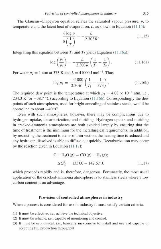
Provision of controlled atmospheres in industry 315
The Clausius–Clapeyron equation relates the saturated vapour pressure, p, totemperature and the latent heat of evaporation, L, as shown in Equation (11.15):
∂ log p
∂
(1
T
) = − L
2.303R. (11.15)
Integrating this equation between T1 and T2 yields Equation (11.16a):
log
(p1
p2
)= − L
2.303R
(1
T1− 1
T2
). (11.16a)
For water p2 = 1 atm at 373 K and L = 41000 J mol−1. Thus
log p1 = −41000
2.30R
(1
T1− 1
373
). (11.16b)
The required dew point is the temperature at which p1 = 4.08 × 10⁻⁴ atm, i.e.,234.3 K (or −38.7 ◦C) according to Equation (11.16b). Correspondingly the dewpoints of such atmospheres, used for bright annealing of stainless steels, would becontrolled to about −40 ◦C.
Even with such atmospheres, however, there may be complications due tohydrogen uptake, decarburization, and nitriding. Hydrogen uptake and nitridingin cracked-ammonia atmospheres are both avoided largely by ensuring that thetime of treatment is the minimum for the metallurgical requirements. In addition,by restricting the treatment to items of thin section, the heating time is reduced andany hydrogen dissolved is able to diffuse out quickly. Decarburization may occurby the reaction given in Equation (11.17):
C + H2O (g) = CO (g) + H2 (g);
�Go17 = 135 00 − 142.6T J. (11.17)
which proceeds rapidly and is, therefore, dangerous. Fortunately, the most usualapplication of the cracked-ammonia atmosphere is to stainless steels where a lowcarbon content is an advantage.
Provision of controlled atmospheres in industry
When a process is considered for use in industry it must satisfy certain criteria.
(1) It must be effective, i.e., achieve the technical objective.(2) It must be reliable, i.e., capable of monitoring and control.(3) It must be economical, i.e., basically inexpensive to install and use and capable of
accepting full production throughput.
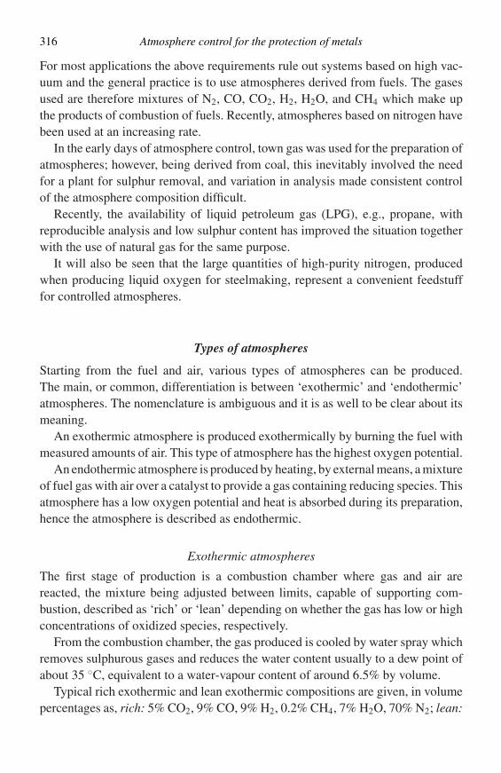
316 Atmosphere control for the protection of metals
For most applications the above requirements rule out systems based on high vac-uum and the general practice is to use atmospheres derived from fuels. The gasesused are therefore mixtures of N2, CO, CO2, H2, H2O, and CH4 which make upthe products of combustion of fuels. Recently, atmospheres based on nitrogen havebeen used at an increasing rate.
In the early days of atmosphere control, town gas was used for the preparation ofatmospheres; however, being derived from coal, this inevitably involved the needfor a plant for sulphur removal, and variation in analysis made consistent controlof the atmosphere composition difficult.
Recently, the availability of liquid petroleum gas (LPG), e.g., propane, withreproducible analysis and low sulphur content has improved the situation togetherwith the use of natural gas for the same purpose.
It will also be seen that the large quantities of high-purity nitrogen, producedwhen producing liquid oxygen for steelmaking, represent a convenient feedstufffor controlled atmospheres.
Types of atmospheres
Starting from the fuel and air, various types of atmospheres can be produced.The main, or common, differentiation is between ‘exothermic’ and ‘endothermic’atmospheres. The nomenclature is ambiguous and it is as well to be clear about itsmeaning.
An exothermic atmosphere is produced exothermically by burning the fuel withmeasured amounts of air. This type of atmosphere has the highest oxygen potential.
An endothermic atmosphere is produced by heating, by external means, a mixtureof fuel gas with air over a catalyst to provide a gas containing reducing species. Thisatmosphere has a low oxygen potential and heat is absorbed during its preparation,hence the atmosphere is described as endothermic.
Exothermic atmospheres
The first stage of production is a combustion chamber where gas and air arereacted, the mixture being adjusted between limits, capable of supporting com-bustion, described as ‘rich’ or ‘lean’ depending on whether the gas has low or highconcentrations of oxidized species, respectively.
From the combustion chamber, the gas produced is cooled by water spray whichremoves sulphurous gases and reduces the water content usually to a dew point ofabout 35 ◦C, equivalent to a water-vapour content of around 6.5% by volume.
Typical rich exothermic and lean exothermic compositions are given, in volumepercentages as, rich: 5% CO2, 9% CO, 9% H2, 0.2% CH4, 7% H2O, 70% N2; lean:
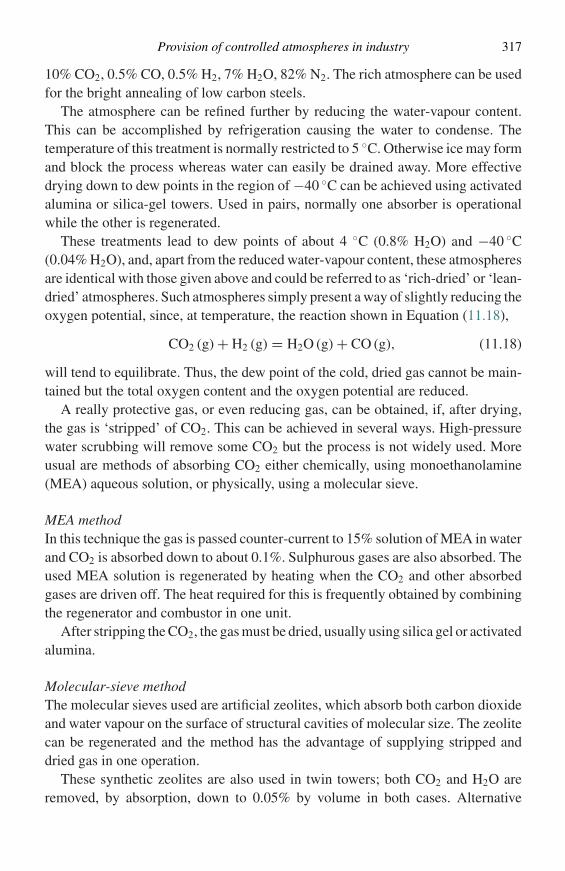
Provision of controlled atmospheres in industry 317
10% CO2, 0.5% CO, 0.5% H2, 7% H2O, 82% N2. The rich atmosphere can be usedfor the bright annealing of low carbon steels.
The atmosphere can be refined further by reducing the water-vapour content.This can be accomplished by refrigeration causing the water to condense. Thetemperature of this treatment is normally restricted to 5 ◦C. Otherwise ice may formand block the process whereas water can easily be drained away. More effectivedrying down to dew points in the region of −40 ◦C can be achieved using activatedalumina or silica-gel towers. Used in pairs, normally one absorber is operationalwhile the other is regenerated.
These treatments lead to dew points of about 4 ◦C (0.8% H2O) and −40 ◦C(0.04% H2O), and, apart from the reduced water-vapour content, these atmospheresare identical with those given above and could be referred to as ‘rich-dried’ or ‘lean-dried’ atmospheres. Such atmospheres simply present a way of slightly reducing theoxygen potential, since, at temperature, the reaction shown in Equation (11.18),
CO2 (g) + H2 (g) = H2O (g) + CO (g), (11.18)
will tend to equilibrate. Thus, the dew point of the cold, dried gas cannot be main-tained but the total oxygen content and the oxygen potential are reduced.
A really protective gas, or even reducing gas, can be obtained, if, after drying,the gas is ‘stripped’ of CO2. This can be achieved in several ways. High-pressurewater scrubbing will remove some CO2 but the process is not widely used. Moreusual are methods of absorbing CO2 either chemically, using monoethanolamine(MEA) aqueous solution, or physically, using a molecular sieve.
MEA methodIn this technique the gas is passed counter-current to 15% solution of MEA in waterand CO2 is absorbed down to about 0.1%. Sulphurous gases are also absorbed. Theused MEA solution is regenerated by heating when the CO2 and other absorbedgases are driven off. The heat required for this is frequently obtained by combiningthe regenerator and combustor in one unit.
After stripping the CO2, the gas must be dried, usually using silica gel or activatedalumina.
Molecular-sieve methodThe molecular sieves used are artificial zeolites, which absorb both carbon dioxideand water vapour on the surface of structural cavities of molecular size. The zeolitecan be regenerated and the method has the advantage of supplying stripped anddried gas in one operation.
These synthetic zeolites are also used in twin towers; both CO2 and H2O areremoved, by absorption, down to 0.05% by volume in both cases. Alternative
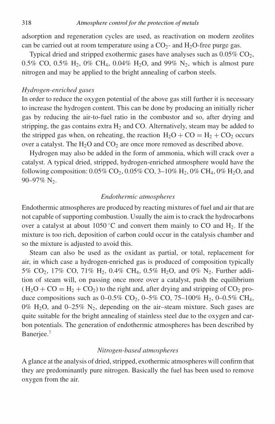
318 Atmosphere control for the protection of metals
adsorption and regeneration cycles are used, as reactivation on modern zeolitescan be carried out at room temperature using a CO2- and H2O-free purge gas.
Typical dried and stripped exothermic gases have analyses such as 0.05% CO2,0.5% CO, 0.5% H2, 0% CH4, 0.04% H2O, and 99% N2, which is almost purenitrogen and may be applied to the bright annealing of carbon steels.
Hydrogen-enriched gasesIn order to reduce the oxygen potential of the above gas still further it is necessaryto increase the hydrogen content. This can be done by producing an initially richergas by reducing the air-to-fuel ratio in the combustor and so, after drying andstripping, the gas contains extra H2 and CO. Alternatively, steam may be added tothe stripped gas when, on reheating, the reaction H2O + CO = H2 + CO2 occursover a catalyst. The H2O and CO2 are once more removed as described above.
Hydrogen may also be added in the form of ammonia, which will crack over acatalyst. A typical dried, stripped, hydrogen-enriched atmosphere would have thefollowing composition: 0.05% CO2, 0.05% CO, 3–10% H2, 0% CH4, 0% H2O, and90–97% N2.
Endothermic atmospheres
Endothermic atmospheres are produced by reacting mixtures of fuel and air that arenot capable of supporting combustion. Usually the aim is to crack the hydrocarbonsover a catalyst at about 1050 ◦C and convert them mainly to CO and H2. If themixture is too rich, deposition of carbon could occur in the catalysis chamber andso the mixture is adjusted to avoid this.
Steam can also be used as the oxidant as partial, or total, replacement forair, in which case a hydrogen-enriched gas is produced of composition typically5% CO2, 17% CO, 71% H2, 0.4% CH4, 0.5% H2O, and 0% N2. Further addi-tion of steam will, on passing once more over a catalyst, push the equilibrium( H2O + CO = H2 + CO2) to the right and, after drying and stripping of CO2 pro-duce compositions such as 0–0.5% CO2, 0–5% CO, 75–100% H2, 0–0.5% CH4,0% H2O, and 0–25% N2, depending on the air–steam mixture. Such gases arequite suitable for the bright annealing of stainless steel due to the oxygen and car-bon potentials. The generation of endothermic atmospheres has been described byBanerjee.5
Nitrogen-based atmospheres
A glance at the analysis of dried, stripped, exothermic atmospheres will confirm thatthey are predominantly pure nitrogen. Basically the fuel has been used to removeoxygen from the air.
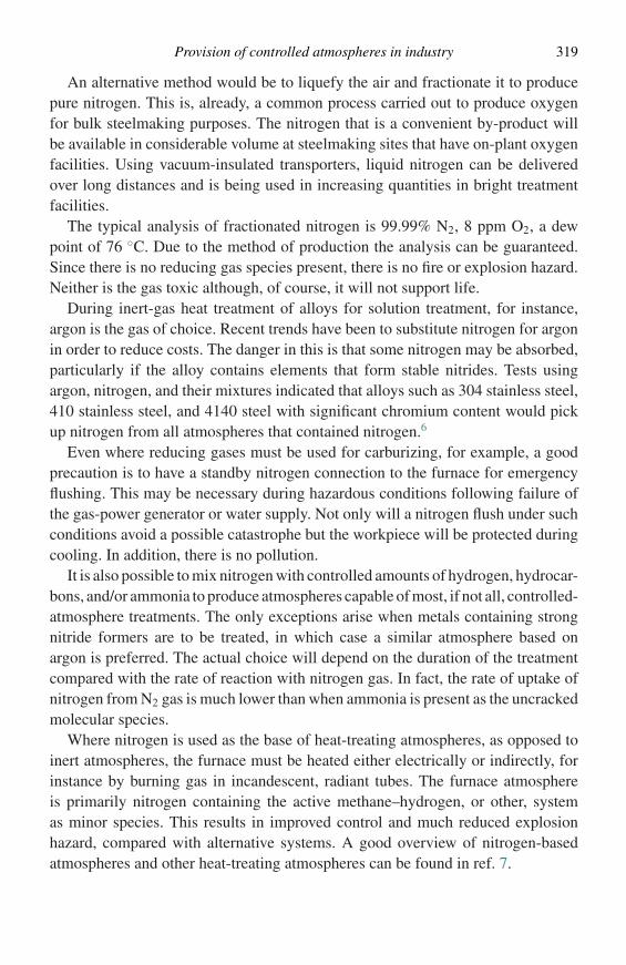
Provision of controlled atmospheres in industry 319
An alternative method would be to liquefy the air and fractionate it to producepure nitrogen. This is, already, a common process carried out to produce oxygenfor bulk steelmaking purposes. The nitrogen that is a convenient by-product willbe available in considerable volume at steelmaking sites that have on-plant oxygenfacilities. Using vacuum-insulated transporters, liquid nitrogen can be deliveredover long distances and is being used in increasing quantities in bright treatmentfacilities.
The typical analysis of fractionated nitrogen is 99.99% N2, 8 ppm O2, a dewpoint of 76 ◦C. Due to the method of production the analysis can be guaranteed.Since there is no reducing gas species present, there is no fire or explosion hazard.Neither is the gas toxic although, of course, it will not support life.
During inert-gas heat treatment of alloys for solution treatment, for instance,argon is the gas of choice. Recent trends have been to substitute nitrogen for argonin order to reduce costs. The danger in this is that some nitrogen may be absorbed,particularly if the alloy contains elements that form stable nitrides. Tests usingargon, nitrogen, and their mixtures indicated that alloys such as 304 stainless steel,410 stainless steel, and 4140 steel with significant chromium content would pickup nitrogen from all atmospheres that contained nitrogen.6
Even where reducing gases must be used for carburizing, for example, a goodprecaution is to have a standby nitrogen connection to the furnace for emergencyflushing. This may be necessary during hazardous conditions following failure ofthe gas-power generator or water supply. Not only will a nitrogen flush under suchconditions avoid a possible catastrophe but the workpiece will be protected duringcooling. In addition, there is no pollution.
It is also possible to mix nitrogen with controlled amounts of hydrogen, hydrocar-bons, and/or ammonia to produce atmospheres capable of most, if not all, controlled-atmosphere treatments. The only exceptions arise when metals containing strongnitride formers are to be treated, in which case a similar atmosphere based onargon is preferred. The actual choice will depend on the duration of the treatmentcompared with the rate of reaction with nitrogen gas. In fact, the rate of uptake ofnitrogen from N2 gas is much lower than when ammonia is present as the uncrackedmolecular species.
Where nitrogen is used as the base of heat-treating atmospheres, as opposed toinert atmospheres, the furnace must be heated either electrically or indirectly, forinstance by burning gas in incandescent, radiant tubes. The furnace atmosphereis primarily nitrogen containing the active methane–hydrogen, or other, systemas minor species. This results in improved control and much reduced explosionhazard, compared with alternative systems. A good overview of nitrogen-basedatmospheres and other heat-treating atmospheres can be found in ref. 7.
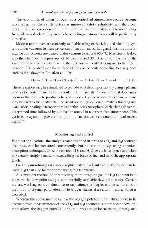
320 Atmosphere control for the protection of metals
The economics of using nitrogen as a controlled-atmosphere source becomemore attractive when such factors as improved safety, reliability, and therefore,productivity are considered.8 Furthermore, the present tendency is to move awayfrom oil towards electricity, in which case nitrogen atmospheres will be particularlyattractive.
Modern techniques are currently available using carburizing and nitriding sys-tems under vacuum. In these processes of vacuum carburizing and plasma carburiz-ing, the components are heated under vacuum to around 950 ◦C. Methane is leakedinto the chamber to a pressure of between 3 and 30 mbar to add carbon to thesystem. In the absence of a plasma, the methane will only decompose to the extentof about 3%, probably on the surface of the components according to a sequencesuch as that shown in Equation (11.19):
CH4 → CH3 + H → CH2 + 2H → CH + 3H → C + 4H. (11.19)
These reactions may be stimulated to provide 80% decomposition by using a plasmaprocess to excite the methane molecule. In this case, the molecular breakdown mayoccur in the plasma to produce charged species. Hydrocarbons other than methanemay be used as the feedstock. The usual operating sequence involves flushing andevacuation, heating to temperature under the inert atmosphere, carburizing for a pre-determined time followed by a diffusion anneal in a carbon-free atmosphere. Thiscycle is designed to provide the optimum surface carbon content and carburizeddepth.9–11
Monitoring and control
For most applications, the analysis can be defined in terms of CO2 and H2O contentand these can be measured conveniently, but not continuously, using chemicalabsorption techniques. Once the correct CO2 and H2O levels have been establishedit is usually simply a matter of controlling the feeds of fuel and air to the appropriatelevels.
For CO2 monitoring on a more sophisticated level, infra-red absorption can beused; H2O can also be monitored using this technique.
A convenient method of continuously monitoring the gas for H2O content is tomeasure the dew point using a commercially available dew-point meter. Certainmeters, working on a conductance or capacitance principle, can be set to controlthe input, or drying, parameters, or to trigger alarms if a certain limiting value isexceeded.
Whereas the above methods allow the oxygen potential of an atmosphere to bededuced from measurements of the CO2 and H2O contents, a more recent develop-ment allows the oxygen potential, or partial pressure, to be measured directly and
Heating methods 321
Figure 11.5 Schematic diagram of an electrochemical cell for monitoring oxygenpartial pressures.
continuously. This technique is based on the use of a high-temperature galvaniccell. The instrument is simply a tube of zirconia stabilized with CaO or Y2O3.Within the tube a known (reference) oxygen partial pressure is imposed either byflushing with a gas of known oxygen potential or by using a metal–metal-oxidemixture. A platinum wire establishes contact with the inner surface of the tube.The tube is then placed in the furnace atmosphere at temperature. Since the stabi-lized zirconia has conductivity for oxygen ions only, the galvanic cell illustrated inFigure 11.5 is established. The free-energy change for the cell reaction is given byEquation (11.20):
�G = RT ln
(p′
O2
p′′O2
). (11.20)
Consequently the emf of the cell is given by Equation (11.21),
E = RT
4Fln
(p′′
O2
p′O2
), (11.21)
where F is Faraday’s constant. In practice, the reference electrode could be con-trolled by flushing air or by establishing a reference oxygen partial pressure by amixture of a suitable metal and its oxide, such as Ni and NiO. Clearly the emf ofsuch a cell can be indicated continuously and also used for feedback to correct thefeed settings of fuel and air.
Difficulties encountered include thermal shock requiring relatively slow heating-and cooling-rates, although if mounted permanently in the furnace these should beachieved. It is important to mount the cell in a position that is exposed to the sametemperature and gas composition as the working volume of the furnace to avoidunrepresentative readings. In addition, the cell will only indicate the equilibriumoxygen partial pressure, regardless of whether or not the atmosphere has equili-brated. This is because the gas will equilibrate locally on the platinum contact ofthe cell.
Heating methods
It is clear that an independent source of heating is essential. Electrical heating isclean, controllable, and simple. Alternatively, gas can be burned within incandescent
322 Atmosphere control for the protection of metals
tubes built into the furnace walls heating by radiation. With atmospheres of highcarbon potential, the possibility of carburizing the electrical heating elements mustalso be considered and suitable shielding arranged.
References
1. O. Kubaschewski, E. H. Evans, and C. B. Alcock, Metallurgical Thermochemistry,Oxford, Pergamon Press, 1967.
2. L. S. Darken and R. W. Gurry, Physical Chemistry of Metals, New York,McGraw-Hill, 1953.
3. F. D. Richardson and J. H. E. Jeffes, J. Iron Steel Inst., 160 (1948), 261.4. T. Ellis, S. Davidson, and C. Bodworth, J. Iron Steel Inst., 201 (1963), 582.5. S. N. Banerjee, Adv. Mater. Proc., 153 (June) (1998), 84SS.6. J. Conybear, Adv. Mater. Proc., 153 (June) (1998), 53.7. P. Johnson, ‘Furnace Atmospheres’. In ASM Handbook, 10th edn, Metals Park, OH,
ASM International, 1991, vol. 4, p. 542.8. R. G. Bowes, Heat Treatment Met., 4, (1975), 117.9. F. Preisser, K. Loser, G. Schmitt, and R. Seeman, ALD Vacuum Technologies
Information, East Windsor, CT.10. F. Schnatbaum and A. Medber, ALD Vacuum Technologies Information, East
Windsor, CT.11. M. H. Jacobs, T. J. Law, and F. Ribet, Surf. Eng., 1 (1985), 105.
Further reading
L. H. Fairbank and L. G. W. Palethorpe, ‘Heat treatment of Metals,’ ISI Special Report.No. 95, London, ISD 1966, p. 57.
R. V. Cutts and H. Dan, Proceedings of the Institute of Iron and Steel Wire ManufacturersConference, Harrogate, March 1972, paper 7.
Appendix A
Solution to Fick’s second law for a semi-infinite solid
Consider an alloy A–B which has B being removed from the surface, e.g., byevaporation. Initially the concentration of B (expressed as mole fraction) will beuniform at N o
B, as indicated in Figure A1(a). If the surface concentration is fixedat a constant value N (S)
B , the concentration profile of B will appear as that in FigureA1(b). For a constant interdiffusion coefficient in the alloy, Fick’s second lawmay be written for this case as in Equation (A1), where D is the interdiffusioncoefficient:
∂ NB
∂ t= D
∂ 2 NB
∂ x2. (A1)
The solution to this equation, following Gaskell,1 can be accomplished by letting
Z = x
2√
Dtso that we obtain Equations (A2) and (A3):
∂ Z
∂ x= 1
2√
Dt, (A2)
∂ Z
∂ t= −x
4√
Dt3. (A3)
Thus, the expressions in Equations (A4) and (A5) are derived:
∂ NB
∂ t= dNB
dZ
∂ Z
∂ t= −x
4√
Dt3
dNB
dZ, (A4)
∂ 2 NB
∂x2= ∂
∂x
[dNB
dZ
∂ Z
∂x
]= d2 NB
dZ2
(∂ Z
∂x
)2
= 1
4Dt
d2 NB
dZ2. (A5)
Substitution of Equations (A4) and (A5) into Equation (A1) yields Equation (A6):
−x/4√
Dt3
dNB
dZ= /
D1/
4/Dt
d2 NB
dZ2. (A6)
323
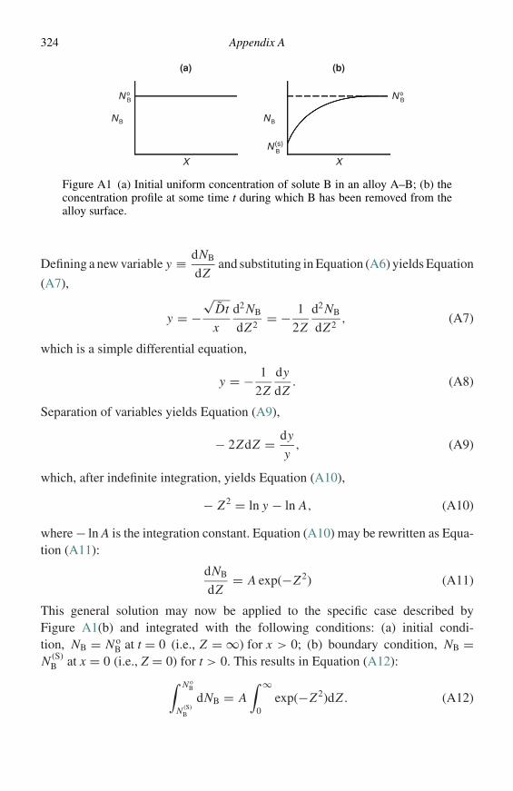
324 Appendix A
N oB N o
B
NB(s)
NB NB
X X
(a) (b)
Figure A1 (a) Initial uniform concentration of solute B in an alloy A–B; (b) theconcentration profile at some time t during which B has been removed from thealloy surface.
Defining a new variable y ≡ dNB
dZand substituting in Equation (A6) yields Equation
(A7),
y = −√
Dt
x
d2 NB
dZ2= − 1
2Z
d2 NB
dZ2, (A7)
which is a simple differential equation,
y = − 1
2Z
dy
dZ. (A8)
Separation of variables yields Equation (A9),
− 2ZdZ = dy
y, (A9)
which, after indefinite integration, yields Equation (A10),
− Z2 = ln y − ln A, (A10)
where − ln A is the integration constant. Equation (A10) may be rewritten as Equa-tion (A11):
dNB
dZ= A exp(−Z2) (A11)
This general solution may now be applied to the specific case described byFigure A1(b) and integrated with the following conditions: (a) initial condi-tion, NB = N o
B at t = 0 (i.e., Z = ∞) for x > 0; (b) boundary condition, NB =N (S)
B at x = 0 (i.e., Z = 0) for t > 0. This results in Equation (A12):∫ N oB
N (S)B
dNB = A∫ ∞
0exp(−Z2)dZ . (A12)
Appendix A 325
The integral on the right-hand side of Equation (A12) is a standard integral withthe value
√π
2 which identifies the constant A as expressed in Equation (A13):
A = 2√π
(N o
B − N (S)B
). (A13)
Substitution of Equation (A13) into Equation (A11) allows integration of Equation(A11) to solve for the concentration profile at any time t > 0:
∫ NB
N oB
dNB =2
(N o
B − N (S)B
)√
π
∫ Z
∞exp(−Z2)dZ . (A14)
Integrating the left-hand side and reversing the limits on the right results inEquation (A15),
NB − N oB = −2
(N o
B − N (S)B
)√
π
∫ ∞
Zexp(−Z2)dZ
= −(N o
B − N (S)B
)erfc(Z ), (A15)
where erfc(Z) is the complementary error function of Z. Reversing the order ofterms to remove the negative sign yields Equation (A16):
NB − N oB
N SB − N o
B
= erfc(Z). (A16)
This may be rearranged to Equations (A17) or (A18),
NB − N (S)B
N oB − N (S)
B
= 1 − NB − N oB
N (S)B − N o
B
= 1 − erfc(Z); (A17)
NB − N (S)B
N oB − N (S)
B
= erf(Z). (A18)
where erf(Z) is the error function of Z which may be found in standard mathematicaltables. Thus, the particular solution for the conditions describing Figure A1 is givenin Equation (A19):
NB = N (S)B + (
N oB − N (S)
B
)erf
(x
2√
Dt
). (A19)
This is a specific case of the general solution to Fick’s second law for diffusion intoor out of a semi-infinite solid, which may be written as in Equation (A20),
NB = A1 + B1 erf
(x
2√
Dt
)(A20)

326 Appendix A
where A1 and B1 are constants which are determined by the initial and boundaryconditions on the particular problem.
Reference
1. D. R. Gaskell, An Introduction to Transport Phenomena in Materials Engineering,New York, Macmillan Publishing Co., 1992, ch. 10.
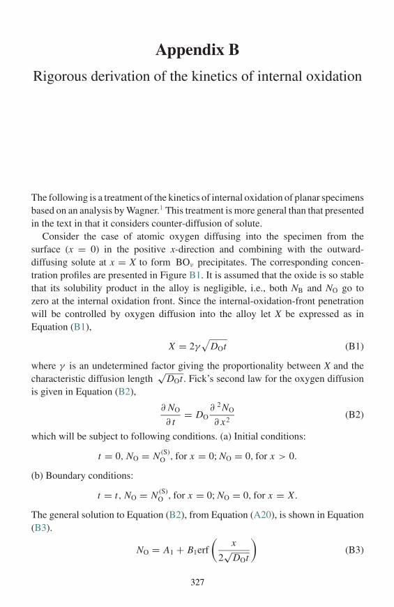
Appendix B
Rigorous derivation of the kinetics of internal oxidation
The following is a treatment of the kinetics of internal oxidation of planar specimensbased on an analysis by Wagner.1 This treatment is more general than that presentedin the text in that it considers counter-diffusion of solute.
Consider the case of atomic oxygen diffusing into the specimen from thesurface (x = 0) in the positive x-direction and combining with the outward-diffusing solute at x = X to form BOν precipitates. The corresponding concen-tration profiles are presented in Figure B1. It is assumed that the oxide is so stablethat its solubility product in the alloy is negligible, i.e., both NB and NO go tozero at the internal oxidation front. Since the internal-oxidation-front penetrationwill be controlled by oxygen diffusion into the alloy let X be expressed as inEquation (B1),
X = 2γ√
DOt (B1)
where γ is an undetermined factor giving the proportionality between X and thecharacteristic diffusion length
√DOt . Fick’s second law for the oxygen diffusion
is given in Equation (B2),
∂ NO
∂ t= DO
∂ 2 NO
∂ x2(B2)
which will be subject to following conditions. (a) Initial conditions:
t = 0, NO = N (S)O , for x = 0; NO = 0, for x > 0.
(b) Boundary conditions:
t = t, NO = N (S)O , for x = 0; NO = 0, for x = X.
The general solution to Equation (B2), from Equation (A20), is shown in Equation(B3).
NO = A1 + B1erf
(x
2√
DOt
)(B3)
327
328 Appendix B
NB(o)
NB
NO
O2
X
NO = NB = 0
A–BA + BOν
Figure B1 Concentration profiles for internal oxidation of A–B.
Solution for A1 and B1 using the boundary conditions yields Equation (B4):
NO = N (S)O
1 −
erf
(x
2√
DOt
)erf(γ )
(B4)
Fick’s second law for the solute diffusion is given in Equation (B5),
∂ NB
∂ t= DB
∂ 2 NB
∂ x2(B5)
subject to the following conditions. (a) Initial conditions:
t = 0, NB = 0, for x < 0; NB = N (o)B , for x > 0.
(b) Boundary conditions:
t = t, NB = 0, for x = X ; NB = N (o)B , for x = ∞.
The general solution to Equation (B5) is given in Equation (B6):
NB = A2 + B2erf
(x
2√
DBt
). (B6)
Solution for A2 and B2 using the boundary conditions yields Equation (B7),
NB = N (o)B −
N (o)B
[1 − erf
(x
2√
DBt
)]erfc(�1/2γ )
, (B7)
Appendix B 329
where � ≡ DO/DB. The internal oxidation kinetics (i.e., γ ) are obtained fromwriting a flux balance at x = X:
limε→0
(−DO
∂ NO
∂ x
)x=X−ε
= ν
(DB
∂ NB
∂ x
)x=X+ε
. (B8)
Differentiating Equation (B4) yields Equation (B9a) or (B9b):(∂ NO
∂ x
)x = X
= N (S)O
/Z
erf(γ )√
π
1/Z
√DOt
exp
( −X2
4DOt
); (B9a)
(∂ NO
∂ x
)x=X
= N (S)O
erf(γ )
1√π
1√DOt
exp(−γ 2
). (B9b)
Differentiating Equation (B7) yields Equations (B10a) or (B10b):(∂ NB
∂x
)x=X
= N (o)B
erfc(�1/2γ )
2�√π
1
2� √DBt
exp
( −X2
4DBt
); (B10a)
(∂ NB
∂x
)x=X
= N (o)B
erfc(�1/2γ )
1√π
1√DBt
exp(−�γ 2). (B10b)
Substitution of Equations (B9b) and (B10b) into the flux balance, Equation (B8),yields Equation (B11a),
−DON (S)
O
erf(γ )√�π√
DOtexp(−γ 2)
= νDBN (o)
B
erfc(�1/2γ√�π )
√DBt
exp(−�γ 2). (B11a)
which may be rearranged to Equation (B11b) or (B11c):
N (S)O
N (o)B
= ν DB
DO
erf(γ )
erfc(�1/2γ )
exp(−�γ 2)
exp(−γ 2)
(DO
DB
)1/2
, (B11b)
N (S)O
N (o)B
= ν
�1/2
erf(γ )
erfc(�1/2γ )
exp(γ 2)
exp(�γ 2
) . (B11c)
Equation (B11c) may be solved numerically for any condition but can be solvedanalytically for two important limiting cases.
Case 1: Negligible counterdiffusion of solute
A situation is often encountered in which solute diffusion is very slow relative tothat of oxygen, and the oxygen solubility is small relative to the solute content of
330 Appendix B
the alloy, i.e.DB
DO� N (S)
O
N oB
� 1, for which γ � 1 and γ �1/2 � 1. This allows the
simplifications of terms in Equation (B11c), shown in Equations (B12)–(B14):
erf(γ ) = 2√π
γ, (B12)
exp(γ 2) = 1 + γ 2 ≈ 1, (B13)
erfc(γ �1/2
) = 2√π
exp(−γ 2�
)2γ �1/2
. (B14)
Insertion of Equations (B12–B14) in Equation (B11) yields Equation (B15a),
N (S)O
N (o)B
= ν
�1/2
(2√πγ)
(1 + γ 2)
2√π
exp(−γ 2�)2γ �1/2 exp(�γ 2)
, (B15a)
which simplifies to Equation (B15b) or (B15c):
N (S)O
N (o)B
= 2ν γ 2; (B15b)
γ =(
N (S)O
2ν N (o)B
)1/2
. (B15c)
Substitution of Equation (B15c) into Equation (B1) gives the front penetration at agiven time as shown in Equation (B16):
X =[
2N (S)O DO
ν N (o)B
t
]1/2
. (B16)
This is the same result obtained using the quasi-steady-state approximationEquation (5.9).
Case 2: Significant counterdiffusion of solute
For cases where the solute counterdiffusion becomes important, the approximationsγ � 1 and γ �1/2 � 1 become valid, and we obtain the expressions given inEquations (B17)–(B19):
erf(γ ) = 2√π
γ, (B17)
erfc(γ �1/2) = 1 − 2√π
γ �1/2 ≈ 1, (B18)
exp(γ 2) ≈ exp(γ 2�) ≈ 1. (B19)
Appendix B 331
Substitution of these equations into Equation (B11c) yields Equations (B20a) and(B20b):
N (S)O
N (o)B
= ν
�1/2
2√πγ
1
(1
1
), (B20a)
γ =√
π�1/2 N (S)O
2ν N (o)B
. (B20b)
A more general treatment of the internal oxidation kinetics has been presented byBohm and Kahlweit2 who modified Wagner’s analysis to include a finite solubilityproduct of the oxide in the alloy matrix. The key differences in this case are thatNB and NO do not go to zero at the reaction front and the concentration of oxygenmaintains finite values into the alloy ahead of the front. The case of oxides withlarge solubility products has been treated by Laflamme and Morral.3
Morral4 has criticized the Wagner analysis and argued that concentration profilessuch as that shown in Figure B1 violate principles of local equilibrium and thatsolute enrichment in the zone of internal oxidation is not possible for the case ofzero solubility product. Analysis of this issue is beyond the scope of this bookbut it should be remarked that many experimental observations are consistent withconclusions based on Wagner’s model.
References
1. C. Wagner, Z. Elektrochem., 63 (1959), 772.2. G. Bohm and M. Kahlweit, Acta met., 12 (1964), 641.3. G. R. Laflamme and J. E. Morral, Acta met., 26 (1978), 1791.4. J. E. Morral, Mater. High Temp., 20 (2003), 275.
Appendix C
Effects of impurities on oxide defect structures
This aspect of the theory of defect structures of non-stoichiometric compoundsis usually covered in the main text of books on high-temperature oxidation. Thesubject of doping is interesting for its own sake, and it is vitally important forthe study of the physical chemistry and electrochemistry of ionic compounds.In the case of an introduction to high-temperature oxidation our opinion is that, sincethe control of oxidation rates by controlling the ionic and electronic transport prop-erties of oxides by impurity solution is not generally used as a technique for thedevelopment of oxidation-resistant alloys, this subject should be dealt with in anappendix. This allows it to be covered adequately without over-emphasizing itsimportance.
In the following discussion ZnO will be used as a typical n-type oxide and NiOas a typical p-type oxide.
Negative (n-type) oxides
The native defect structure of an oxide involving excess cations on interstitial siteswith electrons in the conduction band may be represented as in Equations (C1)and (C2):
ZnO = Zn.i + e′ + 1
2O2 (g), (C1)
ZnO = Zn..i + 2e′ + 1
2O2 (g). (C2)
To represent the addition of a more positive cation to the ZnO lattice, con-sider Al2O3 as the dopant oxide. The solution of Al2O3 in ZnO may occur intwo ways.
(a) The Al3+ ions occupy normal Zn2+-ion lattice sites. Since only two corresponding anionlattice sites are available for the three oxide ions, one must be discharged releasing
332
Appendix C 333
oxygen to the atmosphere and putting two electrons in the conduction band accordingto Equation (C3):
Al2O3 = 2Al.Zn + 2e′ + 2OXO + 1
2O2 (g). (C3)
(b) The introduction of extra electrons to the conduction band upsets the equilibriumbetween them and interstitial zinc ions according to Equations (C1) and (C2). Thus,Al2O3 also dissolves in a manner allowing some interstitial zinc ions to be eliminatedaccording to Equations (C4) or (C5):
Al2O3 + Zn..i = 2Al.Zn + 3OX
O + ZnXZn, (C4)
Al2O3 + Zn.i = 2Al.Zn + e′ + 3OX
O + ZnXZn. (C5)
The overall result of doping ZnO with Al2O3, i.e., the oxide of a higher cationiccharge, is to decrease the concentration of cation interstitials and to increase theconcentration of conduction-band electrons, thus reducing the cationic conductivityand increasing the electronic conductivity. Such an effect would decrease the oxidegrowth rate on an alloy on which such an oxide could form.
To represent the addition of a less positive ion onto the ZnO lattice consider thesolution of lithium oxide, Li2O. This may also occur in two ways.
(a) The two Li+ ions occupy normal Zn2+ cationic sites but only one anion site is occupied.The second anion site is filled by taking O2 from the atmosphere and withdrawingelectrons from the conduction band in order to ionize it:
Li2O + 2e′ + 1
2O2 (g) = 2Li′Zn + 2OX
O. (C6)
(b) Since the removal of conduction-band electrons upsets the equilibrium conditions ofEquations (C1) and (C2), an accompanying mechanism would be for two Li+ ions todisplace a Zn2+ ion from an existing cation site and for oxygen to be evolved accordingto Equations (C7a) or (C7b):
Li2O + 2ZnXZn = 2Li′Zn + 2Zn.
i + 1
2O2 (g), (C7a)
Li2O + 2ZnXZn = 2Li′Zn + OX
O + 2Zn.i. (C7b)
This occurs together with the mechanism of Equation (C6) so as to maintain theequilibrium between conduction-band electrons and interstitial zinc ions.
The net result is to increase the concentration of interstitial zinc ions and reducethe concentration of conduction-band electrons, thus increasing the cationic con-ductivity and reducing the electronic conductivity. Such doping should, therefore,lead to increased oxidation rates.
Similar doping reactions can also occur when the n-type conduction behaviourarises through the existence of anion vacancies such as Equation (C8):
MO = V..O + 2e′ + 1
2O2 (g) + MX
M. (C8)
334 Appendix C
The corresponding doping reactions with Al2O3 would be those shown in Equations(C9) and (C10):
Al2O3 + V..O = 2Al.M + 3OX
O, (C9)
Al2O3 = 2Al.M + 2e′ + 2OXO + 1
2O2 (g). (C10)
The doping reactions with Li2O would be those shown in Equations (C11) and(C12):
Li2O + 2e′ + 1
2O2 (g) = 2Li′M + 2OX
O, (C11)
Li2O = 2Li′M + V..O + OX
O. (C12)
Positive (p-type) oxides
The intrinsic defect structure involving cation vacancies and electron holes can beexpressed, using NiO as an example, as in Equation (C13):
1
2O2 (g) = OX
O + V′′Ni + 2h.. (C13)
The consequences of dissolving cations of higher (e.g., Al3+) and lower (e.g.,Li+) valence than nickel may be considered similarly to the cases of n-type oxidesas follows.
Dissolution of Al2O3 may be achieved in two ways which occur together topreserve the equilibrium of Equation (C13).
(a) Two Al3+ ions occupy normal nickel sites and extra oxygen from Al2O3 is evolved asoxygen gas and contributes two electrons, which neutralize two electron holes:
Al2O3 + 2h. = 2Al.Ni + 2OXO + 1
2O2 (g). (C14)
(b) The two Al3 + ions occupy normal nickel-ion sites and the three oxide-ions can occupynormal oxide-ion sites, thus creating a nickel-ion vacancy, Equation (C15):
Al2O3 = 2Al.Ni + V′′Ni + 3OX
O. (C15)
Thus the dissolution of higher-valence cations into a cation-deficit p-type oxide,such as NiO, leads to creation of more cation vacancies and reduction of the con-centration of electron holes, thus increasing the cation conductivity and decreasingthe electronic conductivity. The net effect would be to increase the oxidation rate,at least in the case where lattice diffusion controls the rate.
The effects of dissolving a cation of lower valence follow similar lines, e.g.,using Li2O one has the following possibilities.
Appendix C 335
(a) The two Li+ ions occupy normal nickel sites, an oxygen atom is ionized from the gasphase to fill the second anion site, and two electron holes are created, Equation (C16):
Li2O + 1
2O2 (g) = 2Li′Ni + 2h. + 2OX
O. (C16)
(b) One of the two Li+ ions occupies a nickel vacancy, Equation (C17):
Li2O + V′′Ni = 2Li′Ni + OX
O. (C17)
The net result is that nickel vacancies are consumed and electron holes areproduced to maintain equilibrium in Equation (C13). Thus the cation conductivityis reduced and electronic conductivity is increased. A corresponding reduction inoxidation rate would be expected.
It is also possible to produce p-type behaviour by having interstitial excess anionsaccording to Equation (C18),
1
2O2(g) = O′′
i + 2h, (C18)
although the number of examples are limited because of the large strain energyassociated with moving a large oxide ion into an interstitial position.
The corresponding dissolution mechanism for Al2O3 and Li2O in a p-type oxideMO with excess anions would be as follows, in order to maintain equilibrium inEquation (C18).
(a) The Al2O3 dissolution could proceed as shown in Equations (C19) and (C20):
Al2O3 = 2Al.M + 2OXO + O′′
i , (C19)
Al2O3 + 2h. = 2Al.M + 2OXO + 1
2O2 (g). (C20)
This will result in increased oxide-ion interstitials and higher ionic conductivity,together with lower concentrations of electron holes and lower electronic conductivity.
(b) The Li2O dissolution could proceed as in Equations (C21) and (C22):
Li2O + O′′i = 2Li′M + 2OX
O, (C21)
Li2O + 1
2O2 (g) = 2Li′M + 2h. + 2OX
O. (C22)
This will produce lower interstitial anion concentrations with correspondinglyreduced ionic conductivity, together with increased electron-hole concentration andassociated increased electronic conductivity.

Index
above-the-pack aluminizing 274accelerated oxidation 132acidic fluxing 213, 225–237activator 272active oxidation 96activity 17activity vs. composition diagram 20Ag–In alloys 114Ag–Zn–Al alloys 115Al2O3 63, 82, 123, 137alkali metals 142alloy depletion 118alloy-induced acidic fluxing 225–230alumina-forming alloys 122–126aluminium oxidation 82aluminizing of nickel-base alloys
272–278APS TBC 287, 298argon-shrouded plasma spraying 151–158Auger electron spectroscopy 14Auger electrons 11automatic recording balance 7
backscattered electrons 11, 12basic fluxing 213, 215–225, 237bond coat 287Bragg’s law 13breakaway oxidation 180buckling 92, 93, 137, 143, 296burner rig 250
carbon penetration through oxides 180carburization 171–172, 320catastrophic oxidation 149–151chemical potentials, equality of 19chemical vapour deposition (CVD) 274chromia-forming alloys 116–122chromium oxidation 94, 137chromized coatings 278cladding 286Clausius–Clapeyron equation 315coating degradation 289–301coating–substrate interdiffusion 289, 291
cobalt oxidation 56–59, 61, 86–87Co–Cr alloys 121Co–Cr–Al alloys 126Co–Cr–Al–Y coating 282common tangent construction 19copper oxidation 59–60, 87Cr2O3 63, 137CrO2(OH)2 182CrO3 evaporation 90–92Cu–Zn–Al alloys 115cyclic oxidation 140
decarburization depth 152, 155decarburization of steels 151–158, 311degradation of oxidation-resistant coatings 289–294degradation of Pt-modified aluminide coatings 289degradation of thermal-barrier coatings 294–301detonation gun 285dew point 314, 320diffusion coatings 271–279dilute gases 67–68doping effect on oxidation 332doping of n-type oxides 332–334doping of p-type oxides 334–335duplex sulphide–oxide scales 189, 190–195
EB-PVD TBC 287, 296electron-beam physical vapour deposition (EB-PVD)
282Ellingham diagrams 22–24, 310endothermic atmosphere 316, 318epitaxial stresses 135equilibrium constant 18erosion of materials 253–255erosion–corrosion 255–269
of alloys 268–269of pure metals 258–268regimes 260
erosion-enhanced oxidation 262erosion-maintained transient oxidation 269error function 325, 327etching 10exothermic atmosphere 316–318
336
Index 337
Fe–Cr alloys 119–121Fe–Cr–Al alloys 126, 137Fe–Cu alloys 127–128Fe–Mo–Al alloys 168Fe–Si Alloys 126Fick’s second law 323, 327flame spraying 285free energy vs. composition diagram 19Frenkel defects 40
galvanizing 279gas phase-induced acidic fluxing 230–237gaseous metal chlorides 243graded seal 144growth stresses 76, 92–93, 133, 134–138,
296
H2–H2O–HCl corrosion 201hafnium oxidation 98hot corrosion 24, 30, 151
degradation sequence 207–210initiation stage of 207, 210–212propagation stage of 209, 212–249sequential propagation modes of 230test methods 250
hot-dip coating 279hot shortness 128
intermetallic compounds, oxidation 129–132internal oxidation 101, 104–115, 135, 198,
240internal oxidation kinetics 105–108, 327–331internal oxide morphology 108–111internal sulphidation 198, 199, 240internal/external oxidation transition 111–115interstitial 42, 43, 44, 55–56, 80inward-growing aluminide coating 273ionically conducting scales 169iron oxidation 65–66, 83–86isothermal stability diagrams 27–33
Kroger–Vink notation 43
leaders 282lean exothermic atmosphere 316linear law 3, 4, 63–66, 98, 150logarithmic law 3, 4, 69–72low-pressure plasma spray (LPPS) 285
marker experiments 78, 167metal dusting 172–173metal–carbon reactions 171–173metal–halogen reactions 169–171metal–nitrogen reactions 173–174metal–sulphide eutectics 165metal–sulphur oxygen systems 183–202metal–sulphur reactions 163–168metastable alumina 123, 124Mo5Si3 130molybdenum oxidation 93MoO3 132, 149
MoSi2 130, 132mounting 9multilayer scale growth 83–90
NaCl effects on hot corrosion 243–244Na2SO4, composition of 211Na–S–O stability diagram 212, 217Nb2Al 130NbAl3 130Nb–Zr alloys 128NiAl 123Ni3Al 123Ni–Al alloys 122–124nickel oxidation 61, 62–63, 78–80Ni–Co alloys 128–129Ni–Co–Cr–Al–Y bond coat 296Ni–Co–Cr–Al–Y coating 285Ni–Cr alloys 116–119Ni–Cr–Al alloys 124–126Ni–Cr–Al–Y coating 282Ni–Mo–Al alloys 168niobium oxidation 98–99, 142Ni–S–O eutectic 194nitrogen-based atmospheres 318–320non-stoichiometric ionic compounds 42–48n-type semiconductors 42–46, 80nucleation 108
Ostwald ripening 105outward-growing aluminide coating 273overlay coatings 279–287oxidation of steels 151–158oxide adherence 144oxide cracking 142oxide growth direction 144oxide maps 124oxide pegs 144oxide solubilities in Na2SO4 213oxide spalling 142, 181, 182oxide vaporization 13–14oxygen probe 321
pack cementation 272, 293parabolic law 3, 4, 49, 167parabolic rate constant 62
conversions of 72–73paralinear oxidation 91, 128, 262permeability 107pesting 132phase diagram
of Fe–C 153of Fe–Cr–O 120of Fe–O 83of Ni–Al 274of Na2SO4–CoSO4 234of Na2SO4–MgSO4 234of Na2SO4–NiSO4 234
photoelectrons 11photostimulated luminescence spectroscopy 142physical vapour deposition 280–282Pilling–Bedworth ratio 134, 142
338 Index
plasma-spray coating 283–285plasma torch 285platinum aluminide bond coat 296platinum oxidation 94point defect stresses 136polishing 10proton defects 182Pt-modified aluminide coating 277Pt–Ni alloys 102–103p-type semiconductors 46–48, 78PVD apparatus 281
Raman spectroscopy 142Rapp–Goto criterion 214, 219, 225, 230rarefied atmospheres 66–67ratcheting 296rational rate constant 72, 166reaction path 186reactive-element effect 144–148reactive-element segregation 144recrystallization 136redox gas mixtures 309redox systems 176residual stress 141, 296response to stress 142Rhines–Wolf mechanism 137rhodium oxidation 94rich exothermic atmosphere 316
scanning electron microscope 9, 12–13Schottky defects 40second law of thermodynamics 17–18secondary electrons 11, 12secondary gettering 115, 126secondary-ion mass spectroscopy 14–15selective oxidation 3, 111, 115, 117, 181selective sulphidation 168short-circuit (grain-boundary) diffusion 63, 79, 93,
137silica-forming alloys 126–127silicide coatings 278silicon oxidation 95–97SiO2 132slurry coating 279specimen geometry effects on stress 137spring balance 5sputtering 286stability diagram, Fe–S–O 192stoichiometric ionic compounds 40–41stress generation 133stress measurement 140–142
stresses in oxides 133–148sulphur gettering 145–147sulphur-induced hot corrosion 237–242sulphur penetration through oxides 195–197sulphur segregation 146
tantalum oxidation 99TBC sintering 299thermal-barrier coating (TBC) 287, 288thermal-expansion coefficient 138, 140thermal stresses 133, 138–140, 296thermally grown oxide (TGO) 287thermodynamic diagrams 18–33Ti–Cr–Al coatings 293tilting technique 141titanium aluminides 131, 293titanium oxidation 97transient oxidation 117, 124, 132, 147transmission electron microscope 13–14tungsten oxidation 93Type I hot corrosion 209, 210, 225, 238,
249Type II hot corrosion 209, 210, 233, 249
unstable interface 103
vacancy 43, 45, 46, 48, 49, 56, 79vacancy injection 136vacancy sinks 144vanadium effects on hot corrosion 246–249vapour species diagrams 24–27voids 136volatile metal halides 169volatile species 90–97volatile species diagram
of Cr–O system 26of Mo–O system 94of Si–O system 95of W–O system 94
Wagner’s model for oxide growth 51water-vapour effects on oxidation 181–182wedging mechanism 143WO3 150wrinkling (rumpling) of coatings 290, 292
X-ray diffraction 9, 13, 141X-ray photoelectron spectroscopy 14
zinc oxidation 55, 80–81zirconium oxidation 98