bis working papers - bank for international settlements · bis working papers are written by...
TRANSCRIPT
BIS Working Papers No 691
Effectiveness of unconventional monetary policies in a low interest rate environment by Andrew Filardo and Jouchi Nakajima
Monetary and Economic Department
January 2018
JEL classification: E43, E44, E52, E58.
Keywords: lending rate, quantitative easing, time-varying parameter VAR model, unconventional monetary policy.

BIS Working Papers are written by members of the Monetary and Economic Department of the Bank for International Settlements, and from time to time by other economists, and are published by the Bank. The papers are on subjects of topical interest and are technical in character. The views expressed in them are those of their authors and not necessarily the views of the BIS.
This publication is available on the BIS website (www.bis.org).
© Bank for International Settlements 2018. All rights reserved. Brief excerpts may be reproduced or translated provided the source is stated.
ISSN 1020-0959 (print) ISSN 1682-7678 (online)
1
Effectiveness of unconventional monetary policies in a low interest rate environment†
Andrew Filardo* and Jouchi Nakajima*
Abstract Have unconventional monetary policies (UMPs) become less effective at stimulating economies in persistently low interest rate environments? This paper examines that question with a time-varying parameter VAR for the United States, the United Kingdom, the euro area and Japan. One advantage of our approach is the ability to measure an economy’s evolving interest rate sensitivity during the post-GFC macroeconomy. Another advantage is the ability to capture time variation in the “natural”, or steady state, rate of interest, which allows us to separate interest rate movements that are associated with changes in the stance of monetary policy from those that are not.
We find that UMPs became less effective in the post-GFC period, but not for the reasons typically given. The explanation is nuanced and emerges from careful assessment of the various links in the monetary transmission mechanism. First, our results are consistent with past event studies showing less “bang for the buck” over time from UMPs, ie the diminished impact over time of a given central bank balance sheet change on interest rates. Second, the effect of UMPs on lending rates is slower than on sovereign yields but eventually lending rates and sovereign yields move in tandem. Third, somewhat surprisingly, we find little evidence of a change in the interest sensitivity of the economy once we control for changes in the “natural” rate of interest. Fourth, and most important, our estimates suggest that changes in “natural” rate estimates co-move with unexpected changes in UMPs, contrary to conventional natural rate theory. Taken at face value, this suggests that measured “natural” rates will increase as central banks normalise policy and raise the risk of central banks falling behind the curve. Conceptually, signalling and safe asset mechanisms may account for these findings.
JEL classification: E43, E44, E52, E58.
Keywords: lending rate, quantitative easing, time-varying parameter VAR model, unconventional monetary policy.
† We would like to thank Tobias Adrian, Carlo Altavilla, Claudio Borio, Fabio Canova, Dietrich
Domanski, Matthew Higgins, Boris Hofmann, Jonathan Kearns, Marco Lombardi, Elmar Mertens, Phurichai Rungcharoenkitkul, Pierre Siklos, Nathan Sussman, Mike West, Ji Zhang and seminar participants at the Bank of England, European Central Bank, Duke University, Federal Reserve Bank of New York, the Hong Kong Monetary Authority-Federal Reserve Bank of Atlanta-Federal Reserve System Board of Governors conference on “Unconventional Monetary Policy: Lessons Learned”, the International Monetary Fund, Norges Bank, the Vienna University of Economics and Business, the 10th International Conference on Computational and Financial Econometrics and the Bank for International Settlements for their insightful comments. We also thank Bilyana Bogdanova and Matthias Loerch for their excellent research assistance. All errors are ours.
* Bank for International Settlements.
2
1. Introduction
The Great Financial Crisis (GFC) ushered in a new chapter in the history of central banking. Major central banks in advanced economies addressed the GFC challenges by first cutting policy rates sharply and, when the room for manoeuvre closed, resorting to a range of unconventional monetary policies (UMPs) that exploited the financial firepower of central bank balance sheets. The lacklustre recovery that followed has naturally raised questions about the effectiveness of these new tools.1 Did the economy become less interest rate-sensitive in the aftermath of the GFC or did the new tools prove to be less effective after stress in financial markets faded?
The extant research on effectiveness has reached mixed conclusions. Some microeconomic studies find evidence suggesting an impaired bank lending channel in a low interest rate environment. The flattening of the yield curve and the general reluctance to introduce negative retail deposit rates squeezes net interest margins (eg Borio et al (2015), EIOPA (2014)). But the impact on bank profitability is less clear. Even though shrinking margins hit the bottom line, lower rates improve asset quality. Indeed, central banks which implemented negative policy rates have seen bank equity valuations rise along with profitability.
Macroeconomic studies have also delivered a range of estimated UMP impacts. For example, Panizza and Wyplosz (2016) document diminishing policy rate effectiveness over time for the major advanced economies but little decline in the effectiveness of UMPs. Bech et al (2014) also report that monetary policy is less effective in periods following a financial crisis, while Dahlhaus (2014) notes the beneficial effects of monetary policy during periods of high financial stress.
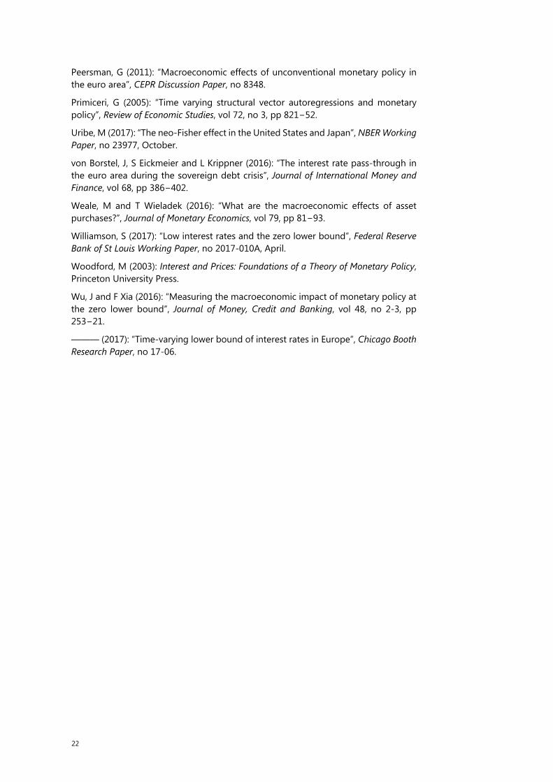
Our study can be seen as trying to bridge this divide by investigating the time-varying strength of the key links in the monetary transmission mechanism, starting from the implementation of UMPs. It stresses the sequence of links from UMPs to sovereign yields to bank lending rates and ultimately to output growth and inflation. In contrast to earlier empirical macro research on the effectiveness of UMPs, we add a link through the bank lending rate. This is motivated in large part by the observation that bank lending rates did not move in lock-step with sovereign yields during the UMP period (Graph 1), thereby suggesting that the pass-through to bank lending rates was gradual. In this sense, our paper is closest to new research by Albertazzi et al (2016), Altavilla et al (2016a) and Von Borstel et al (2016).2
From a modelling perspective, our paper captures the dynamics of the UMP transmission mechanism with a Bayesian time-varying parameter VAR (TVP-VAR) approach. One advantage is that this approach allows us to separate the UMP pass-through into movements in the short-term “natural” rate of interest and into the deviations around this rate. This lets us test whether the cross-country experiences with UMPs are more consistent with the interest sensitivity hypothesis or the policy ineffectiveness hypothesis. One major challenge is data requirements to estimate the two components over a relatively short period of time. To conserve degrees of freedom, we identify monetary policy shocks in a first step of our analysis using an event study approach in the spirit of Kuttner (2004): the UMP shocks are measured
1 Many studies have investigated the effectiveness of the UMP. See Borio and Zabai (2016), Haldane
et al (2016) and Lombardi and Siklos (2017) for recent surveys.
2 Also see Weale and Wieladek (2016), Kapetanios et al (2012), Baumeister and Benati (2013), Kimura and Nakajima (2016), Gambacorta, Hofmann and Peersman (2014), Chen et al (2012), Panniza and Wyplosz (2016), Gambacorta, Illes and Lombardi (2014) and Illes et al (2015).
3
as a change in sovereign bond yields at the time of significant UMP announcements (also see Chen et al (2016, 2017), BIS (2016, Chapter IV)).
We find evidence supporting the hypothesis that the economy did not become less interest-sensitive in the aftermath of the GFC, once changes in the “natural” rate of interest are taken into account. This conclusion is based on impulse response analysis and posterior odds tests of the two hypotheses (ie interest insensitivity versus policy ineffectiveness). In particular, our evidence indicates that the stimulative impact of UMPs via sovereign yields on bank lending rates changed little in the aftermath of the GFC when compared with the pre-GFC period.
To reconcile this evidence with the lacklustre global recovery, we note that estimates of the time-varying “natural”, or steady state, interest rate co-move systematically with UMP shocks. This blunts the cyclical impact of UMPs.3 In addition, the sensitivity of “natural” rate estimates to unexpected changes in UMPs is inconsistent with conventional natural rate theory. What might account for this unexpected sensitivity? We argue that the systematic decline in the estimated “natural” rate of interest to UMP shocks can be explained by a (distorted) signalling or scarcity of safe asset effect.
However, it should be noted that the link in the transmission mechanism from the central bank balance sheet to sovereign yields, since UMPs were first introduced, appears to have weakened over time. Larger and larger balance sheet programmes were needed to push sovereign yields down by a given amount. To the extent that financial market surprises are an important part of the monetary transmission mechanism, the declining “bang for the buck” indicates a weakening of the central bank balance sheet instrument of monetary policy over time.
Overall, by incorporating the UMP monetary policy transmission link through bank lending rates in our analysis, we conclude that UMPs had a declining impact on economies over time. Taken at face value, the results suggest that the attractiveness of using UMPs in the future would have to include an assessment of their time-varying impacts. Naturally, any complete assessment would also have to factor in the unintended costs of UMPs, as documented elsewhere. Looking forward, our results suggest that the normalisation of balance sheet policies could be accompanied by an increase in the conventionally estimated “natural” rate, which if not taken into account would increase the risk that central banks will find themselves falling behind the curve.
The rest of the paper is organised as follows. Section 2 highlights key links in the monetary transmission mechanism to be investigated, including some baseline UMP pass-through estimates to market rates using a fixed parameter VAR model for the United States, the United Kingdom, the euro area and Japan. Section 3 describes our TVP-VAR econometric methodology. Section 4 reports the results from the TVP-VAR model. Section 5 discusses the monetary policy implications of the finding. Section 6 concludes.
3 Note, as the steady state rate declines, a given decline in market rates has a smaller intertemporal
impact. Wealth effects from distributional channels would nonetheless still operate, at least in theory. Hence monetary policy would be less stimulative for a given change in the policy rate or, at the effective lower bound, for a given change in the so-called shadow policy rate.
4
2. The pass-through of UMPs via bank lending rates
2.1 Links in the monetary transmission mechanism
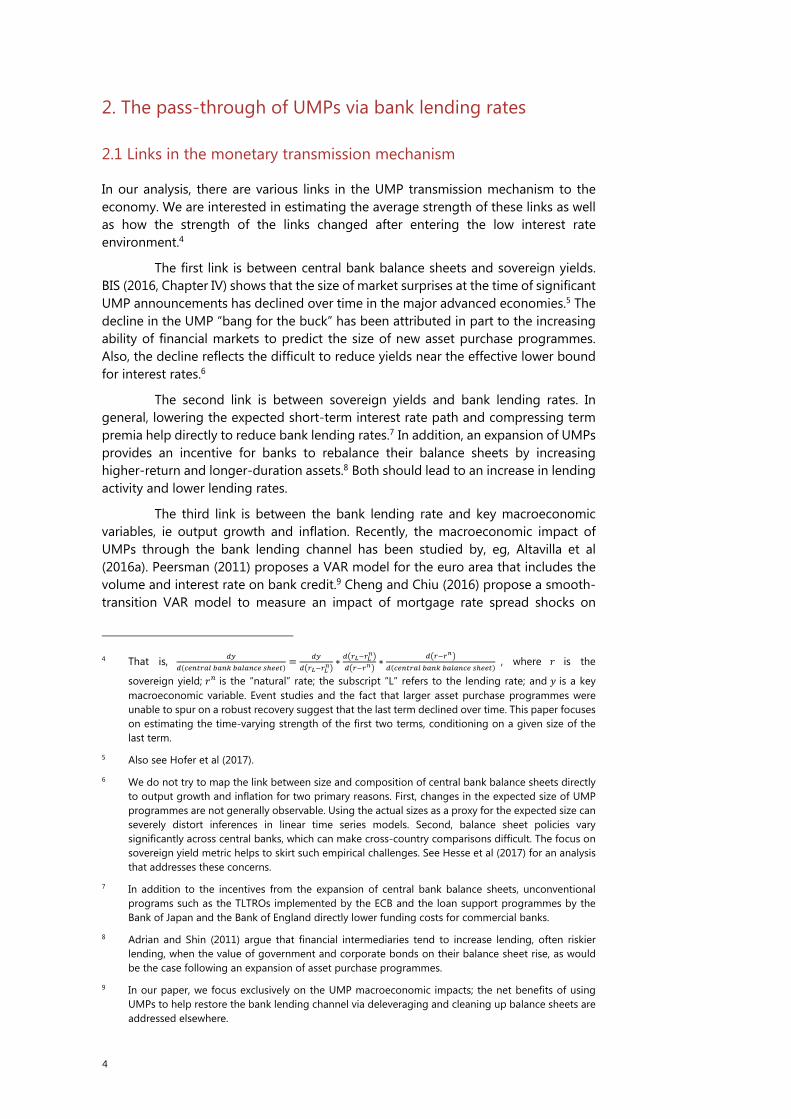
In our analysis, there are various links in the UMP transmission mechanism to the economy. We are interested in estimating the average strength of these links as well as how the strength of the links changed after entering the low interest rate environment.4
The first link is between central bank balance sheets and sovereign yields. BIS (2016, Chapter IV) shows that the size of market surprises at the time of significant UMP announcements has declined over time in the major advanced economies.5 The decline in the UMP “bang for the buck” has been attributed in part to the increasing ability of financial markets to predict the size of new asset purchase programmes. Also, the decline reflects the difficult to reduce yields near the effective lower bound for interest rates.6
The second link is between sovereign yields and bank lending rates. In general, lowering the expected short-term interest rate path and compressing term premia help directly to reduce bank lending rates.7 In addition, an expansion of UMPs provides an incentive for banks to rebalance their balance sheets by increasing higher-return and longer-duration assets.8 Both should lead to an increase in lending activity and lower lending rates.
The third link is between the bank lending rate and key macroeconomic variables, ie output growth and inflation. Recently, the macroeconomic impact of UMPs through the bank lending channel has been studied by, eg, Altavilla et al (2016a). Peersman (2011) proposes a VAR model for the euro area that includes the volume and interest rate on bank credit.9 Cheng and Chiu (2016) propose a smooth-transition VAR model to measure an impact of mortgage rate spread shocks on
4 That is, ( ) = ∗ ∗ ( ) , where is the
sovereign yield; is the “natural” rate; the subscript “L” refers to the lending rate; and is a key macroeconomic variable. Event studies and the fact that larger asset purchase programmes were unable to spur on a robust recovery suggest that the last term declined over time. This paper focuses on estimating the time-varying strength of the first two terms, conditioning on a given size of the last term.
5 Also see Hofer et al (2017).
6 We do not try to map the link between size and composition of central bank balance sheets directly to output growth and inflation for two primary reasons. First, changes in the expected size of UMP programmes are not generally observable. Using the actual sizes as a proxy for the expected size can severely distort inferences in linear time series models. Second, balance sheet policies vary significantly across central banks, which can make cross-country comparisons difficult. The focus on sovereign yield metric helps to skirt such empirical challenges. See Hesse et al (2017) for an analysis that addresses these concerns.
7 In addition to the incentives from the expansion of central bank balance sheets, unconventional programs such as the TLTROs implemented by the ECB and the loan support programmes by the Bank of Japan and the Bank of England directly lower funding costs for commercial banks.
8 Adrian and Shin (2011) argue that financial intermediaries tend to increase lending, often riskier lending, when the value of government and corporate bonds on their balance sheet rise, as would be the case following an expansion of asset purchase programmes.
9 In our paper, we focus exclusively on the UMP macroeconomic impacts; the net benefits of using UMPs to help restore the bank lending channel via deleveraging and cleaning up balance sheets are addressed elsewhere.
5
macroeconomic variables in the United States, differentiating between the impact during recessions and expansions.
The paper’s main contribution is its focus on the empirical strength in the major advanced economies of the second and third links in the low interest rate environment. The focus on the lending rate links in the monetary transmission mechanism sheds some new light on the way UMPs influenced the economy.
2.2 Baseline UMP pass-through estimates to market interest rates
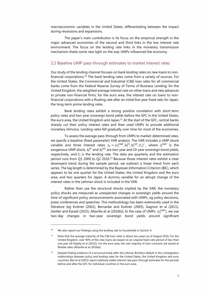
Our study of the lending channel focuses on bank lending rates on new loans to non-financial corporations.10 The bank lending rates come from a variety of sources. For the United States, the Commercial and Industrial (C&I) loan rates for all commercial banks come from the Federal Reserve Survey of Terms of Business Lending; for the United Kingdom, the weighted average interest rate on other loans and new advances to private non-financial firms; for the euro area, the interest rate on loans to non-financial corporations with a floating rate after an initial five-year fixed rate; for Japan, the long-term prime lending rates.
Bank lending rates exhibit a strong positive correlation with short-term policy rates and two-year sovereign bond yields before the GFC in the United States, the euro area, the United Kingdom and Japan.11 At the start of the GFC, central banks sharply cut their policy interest rates and then used UMPs to provide additional monetary stimulus. Lending rates fell gradually over time for most of the economies.
To assess the average pass-through from UMPs to market-determined rates, we specify a baseline (fixed parameter) VAR analysis. The VAR includes a UMP shock variable and three interest rates: = ( , , , ℓ )′ , where is the exogenous UMP shock, and are two-year and 10-year sovereign bond yields, respectively, and ℓ is the lending rate. The data are quarterly and the estimation period runs from Q1 2000 to Q2 2016.12 Because those interest rates exhibit a clear downward trend during the sample period, we subtract a linear trend from each series. The lag length is determined by the Bayesian Information Criterion (BIC), which appears to be one quarter for the United States, the United Kingdom and the euro area, and two quarters for Japan. A dummy variable for an abrupt change of the interest rates in the Lehman shock is included in the VAR.
Rather than use the structural shocks implied by the VAR, the monetary policy shocks are measured as unexpected changes in sovereign yields around the time of significant policy announcements associated with UMPs, eg policy decisions, press conferences and speeches. This methodology has been extensively used in the literature (eg Kuttner (2001), Bernanke and Kuttner (2005), Gagnon et al (2011), Gertler and Karadi (2015), Altavilla et al (2016b)). In the case of UMPs ( ), we use two-day changes in two-year sovereign bond yields around significant
10 We also report our findings using the lending rate to households in Section 4.
11 Note that the average maturity of the C&I loan rates is about two years as of August 2016. For the United Kingdom, over 90% of the new loans are based on an original fixed-rate period of less than one year (Al-Dejaily et al (2012)). For the euro area, the vast majority of loan contracts are issued at flexible rates (Altavilla et al (2016a)).
12 Despite finding evidence of a structural break after the Lehman Brothers default in the cointegration relationships between policy and lending rates for the United States, the United Kingdom and euro countries, Illes et al (2015) report relatively stable interest rate pass-through estimates for the periods before and after the GFC for individual countries in the euro area.

6
announcement dates. Note that this UMP shock is zero before 2007 for the United States, the United Kingdom and the euro area (see Appendix 1).
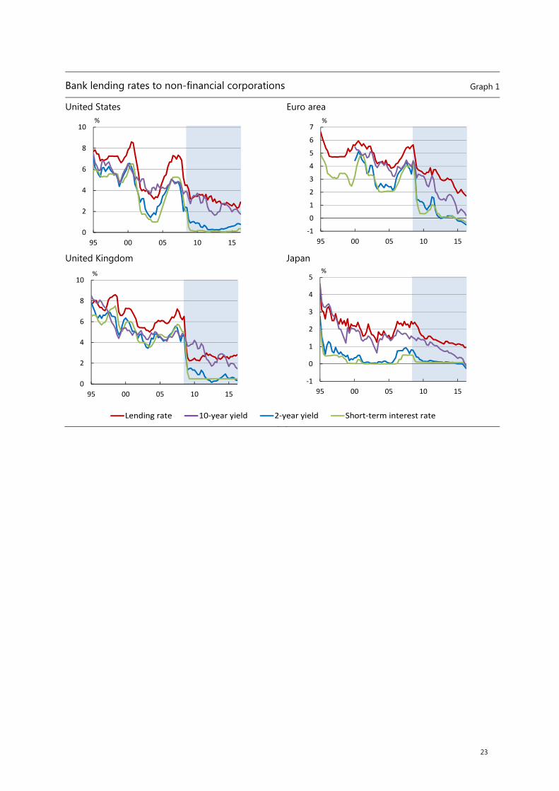
Graph 2 shows the impulse responses of interest rates to a UMP shock; the UMP shock is normalised to be equivalent to a 10 basis point decline in the two-year sovereign yield. The impulse responses show a clear interest-rate pass-through to lending rates during the UMP period. A UMP shock leads to a roughly 0–30 bp decline in market-determined interest rates. For the United States, the United Kingdom and Japan, the lending rates decline more slowly than the sovereign bond yields do, and reach a trough within four quarters. The same pattern of the lending rate responses is observed for the euro area, with the response of sovereign bond yields being more gradual than in other countries. At the trough, the lending rate declines by 30–40 bp following the 10 bp UMP shock, which is a deeper decline than that seen in the sovereign bond yields.13, 14
3. Time-varying parameter VAR framework
3.1. Model
Building on the approach of Primiceri (2005), Giannone et al (2008), Koop et al (2009), and Baumeister and Peersman (2013), we extend the standard TVP-VAR model by adding a set of exogenous UMPs shocks. For a ( × 1) vector of macroeconomic variables , our TVP-VAR model takes the following form:
= + + + , ~ (0, Ω ), where is the ( × 1) vector of time-varying intercept; is the ( × ) matrix of time-varying coefficients for lag variables; is the scalar of exogenous UMP shocks; is the ( × 1) vector of coefficients; and is the ( × 1) vector of reduced-form residuals. The ( × ) covariance matrix of the residuals, Ω , is time-varying and decomposed as Ω = ( )′, where is the diagonal matrix with variances of structural shocks lined in its diagonals; and is the lower-triangular matrix with all the diagonals equal to one, ie a time-varying version of the standard Cholesky-type shock identification strategy. The structural shocks, denoted by , are estimated from the transformation, = , where ~ (0, ).
The exogeneity assumption of the UMP shock, , is key to reducing the dimensionality of the econometrics problem. The coefficient measures a
13 Consistent with our baseline results, ECB (2017) notes that lending rates in major euro area countries
declined more than market steady state rates in the aftermath of the 2014 announcement of the credit easing policy. The decline was interpreted as evidence of an effective interest rate pass-through. Our findings are also consistent with other studies that document significant interest rate pass-through to lending rates during the UMP period. The confidence interval for the euro area in our result is quite large partly because we use the averaged euro area lending rate despite a large diversity of the lending rate among euro area countries. A complemental analysis using the German lending rate provides a narrower confidence interval and higher pass-through than the baseline result based on the euro area average.
14 Because nominal interest rates hit zero during most of the UMP period, non-linear dynamics may result, which could significantly bias the impulse response estimated with the linear VAR system. We address this possibility in the next section by imposing parameter restrictions implied by the effective lower bound.
7
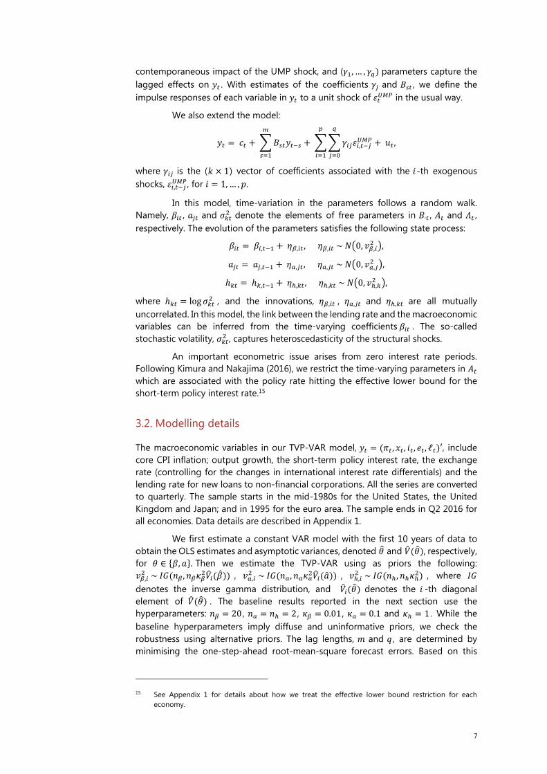
contemporaneous impact of the UMP shock, and ( , … , ) parameters capture the lagged effects on . With estimates of the coefficients and , we define the impulse responses of each variable in to a unit shock of in the usual way.
We also extend the model:
= + + , + , where is the ( × 1) vector of coefficients associated with the -th exogenous shocks, , , for = 1,… , .
In this model, time-variation in the parameters follows a random walk. Namely, , and denote the elements of free parameters in ∙ , and , respectively. The evolution of the parameters satisfies the following state process: = , + , , , ~ 0, , , = , + , , , ~ 0, , , ℎ = ℎ , + , , , ~ 0, , , where ℎ = log , and the innovations, , , , and , are all mutually uncorrelated. In this model, the link between the lending rate and the macroeconomic variables can be inferred from the time-varying coefficients . The so-called stochastic volatility, , captures heteroscedasticity of the structural shocks.
An important econometric issue arises from zero interest rate periods. Following Kimura and Nakajima (2016), we restrict the time-varying parameters in which are associated with the policy rate hitting the effective lower bound for the short-term policy interest rate.15
3.2. Modelling details
The macroeconomic variables in our TVP-VAR model, = ( , , , , ℓ )′, include core CPI inflation; output growth, the short-term policy interest rate, the exchange rate (controlling for the changes in international interest rate differentials) and the lending rate for new loans to non-financial corporations. All the series are converted to quarterly. The sample starts in the mid-1980s for the United States, the United Kingdom and Japan; and in 1995 for the euro area. The sample ends in Q2 2016 for all economies. Data details are described in Appendix 1.
We first estimate a constant VAR model with the first 10 years of data to obtain the OLS estimates and asymptotic variances, denoted and ( ), respectively, for ∈ { , }. Then we estimate the TVP-VAR using as priors the following: , ~ ( , ( )) , , ~ ( , ( )) , , ~ ( , ) , where denotes the inverse gamma distribution, and ( ) denotes the -th diagonal element of ( ) . The baseline results reported in the next section use the hyperparameters: = 20 , = = 2 , = 0.01 , = 0.1 and = 1 . While the baseline hyperparameters imply diffuse and uninformative priors, we check the robustness using alternative priors. The lag lengths, and , are determined by minimising the one-step-ahead root-mean-square forecast errors. Based on this
15 See Appendix 1 for details about how we treat the effective lower bound restriction for each
economy.

8
metric, = 1 for all the economies, and = 2 for the United States, = 1 for the United Kingdom, = 4 for the euro area, and = 2 for Japan.
We use Markov chain Monte Carlo (MCMC) methods to estimate the model following Primiceri (2005) and Nakajima (2011), modified to account for the exogenous monetary policy shocks (ie the additional parameters (sampled with linear regressions) associated with the UMP shocks). The model is estimated with 50,000 iterations after a burn-in period of 10,000. The reported impulse responses are the estimated posterior means, along with 50% confidence intervals.
One drawback of our TVP-VAR analysis with a relatively small sample is that the coefficients are assumed to be constant over time. This assumption reduces the risks of overfitting the data. To test for the reasonableness of this assumption, we segment the UMP announcements for the United States and Japan into subsets, { , } , and test for the time-variation in the coefficients, .
4. Empirical results
4.1. Cross-country evidence
This section reports cross-country evidence on the UMP transmission mechanism for the United States, Japan, the euro area and the United Kingdom using the TVP-VAR model. The stimulative UMP shock used in the impulse responses is normalised to be equivalent to a 10 basis point decline in the two-year sovereign yield. The shapes of the impulse responses are time-varying; hence we label the responses by date corresponding to the value of the estimated parameters of the TVP-VAR for that date.16
4.1.1 United States
For the United States, the long experience with UMPs and the many UMP announcements allow us to divide the UMP period into two subperiods. Specifically, we define the subperiods as (1) LSAP1 and LSAP2 and (2) MEP and LSAP3. Correspondingly, we define the period-specific UMP shocks to be and and the associated coefficients, , for = 1 and 2. Based on our baseline results, we use the UMP shocks from two-year yields for , and from 10-year yields for . This choice reflects the near-zero two-year yields in the second subperiod.
Graph 3(a) presents the impulse responses of the lending rates to UMP shocks for the two highlighted dates.17 The responses are little changed across time, even when we allow for different . 18 The initial impact is about 10 bp and subsequently declines to 30 bp at its trough after two quarters. The shape of the response is similar to that in Altavilla et al (2016a), and the size of the response is
16 The impulse response is computed using the temporal snapshot of time-varying parameters as local
approximation and does not take expectations for future variation in parameters into account.
17 The impulse response includes a decline of the time-varying intercept following the UMP shock. We regress the UMP shocks on the estimated time-varying intercept and compute its response to a –10 bp UMP shock.
18 Note that the response of the lending rate in the initial quarter of the shock is time-invariant, ie the same at the two different dates within each subperiod because the coefficient, , associated with the UMP shock was assumed to be constant.
9
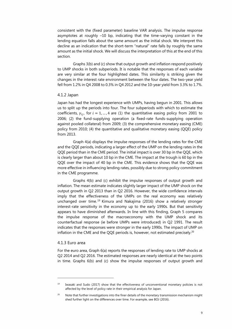
consistent with the (fixed parameter) baseline VAR analysis. The impulse response asymptotes at roughly –10 bp, indicating that the time-varying constant in the lending equation falls about the same amount as the initial shock. We interpret this decline as an indication that the short-term “natural” rate falls by roughly the same amount as the initial shock. We will discuss the interpretation of this at the end of this section.
Graphs 3(b) and (c) show that output growth and inflation respond positively to UMP shocks in both subperiods. It is notable that the responses of each variable are very similar at the four highlighted dates. This similarity is striking given the changes in the interest rate environment between the four dates. The two-year yield fell from 1.2% in Q4 2008 to 0.3% in Q4 2012 and the 10-year yield from 3.3% to 1.7%.
4.1.2 Japan
Japan has had the longest experience with UMPs, having begun in 2001. This allows us to split up the periods into four. The four subperiods with which to estimate the coefficients, , for = 1,… , 4 are (1) the quantitative easing policy from 2001 to 2006; (2) the fund-supplying operation (a fixed-rate funds-supplying operation against pooled collateral) from 2009; (3) the comprehensive monetary easing (CME) policy from 2010; (4) the quantitative and qualitative monetary easing (QQE) policy from 2013.
Graph 4(a) displays the impulse responses of the lending rates for the CME and the QQE periods, indicating a larger effect of the UMP on the lending rates in the QQE period than in the CME period. The initial impact is over 30 bp in the QQE, which is clearly larger than about 10 bp in the CME. The impact at the trough is 60 bp in the QQE over the impact of 40 bp in the CME. This evidence shows that the QQE was more effective in influencing lending rates, possibly due to strong policy commitment in the CME programme.
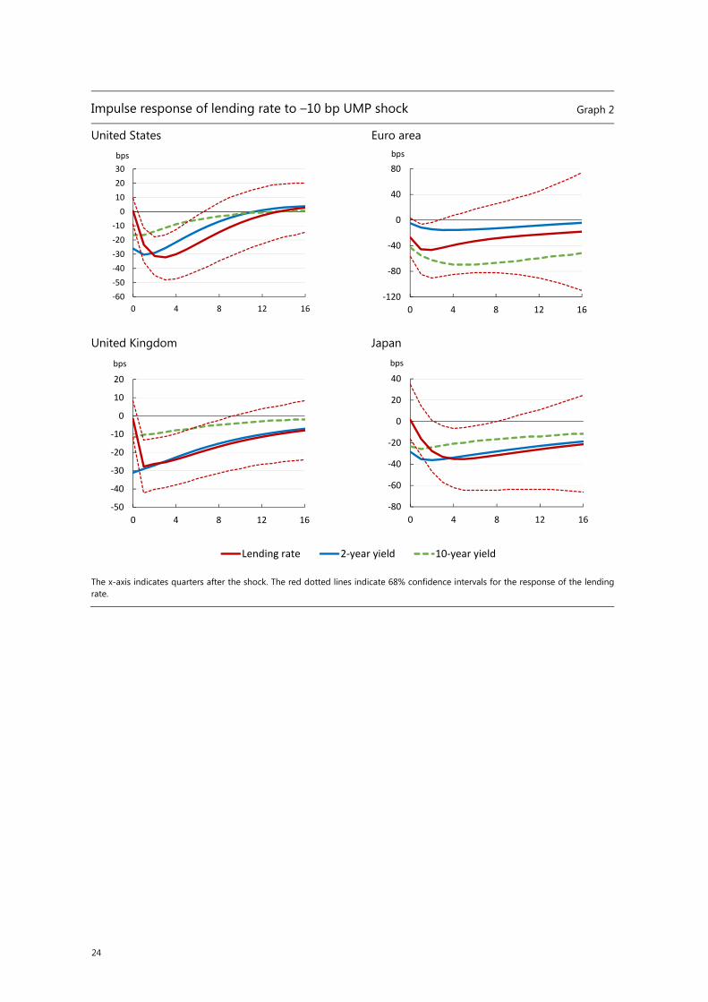
Graphs 4(b) and (c) exhibit the impulse responses of output growth and inflation. The mean estimate indicates slightly larger impact of the UMP shock on the output growth in Q2 2013 than in Q2 2016. However, the wide confidence intervals imply that the effectiveness of the UMPs on the real economy was relatively unchanged over time. 19 Kimura and Nakajima (2016) show a relatively stronger interest-rate sensitivity in the economy up to the early 1990s. But that sensitivity appears to have diminished afterwards. In line with this finding, Graph 5 compares the impulse response of the macroeconomy with the UMP shock and its counterfactual response (ie before UMPs were introduced) in Q2 1991. The result indicates that the responses were stronger in the early 1990s. The impact of UMP on inflation in the CME and the QQE periods is, however, not estimated precisely.20
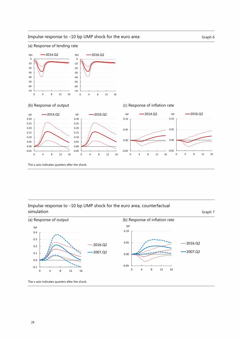
4.1.3 Euro area
For the euro area, Graph 6(a) reports the responses of lending rate to UMP shocks at Q2 2014 and Q2 2016. The estimated responses are nearly identical at the two points in time. Graphs 6(b) and (c) show the impulse responses of output growth and
19 Iwasaki and Sudo (2017) show that the effectiveness of unconventional monetary policies is not
affected by the level of policy rate in their empirical analysis for Japan.
20 Note that further investigations into the finer details of the monetary transmission mechanism might shed further light on the differences over time. For example, see BOJ (2016).
10
inflation to the UMP shock. Both variables respond positively, although the response of the inflation rate is much more gradual.
Graph 7 compares the impulse response of the macroeconomic variables for Q2 2016 and Q2 2007, when the sovereign yield curve was much higher. The counterfactual response on output growth for Q2 2007 differs little from that nine years later, despite the changes in the economy pre- and post-crisis. However, inflation appears much more muted and consistent with evidence of a flattening of the Phillips curve found in other studies.
4.1.2 United Kingdom
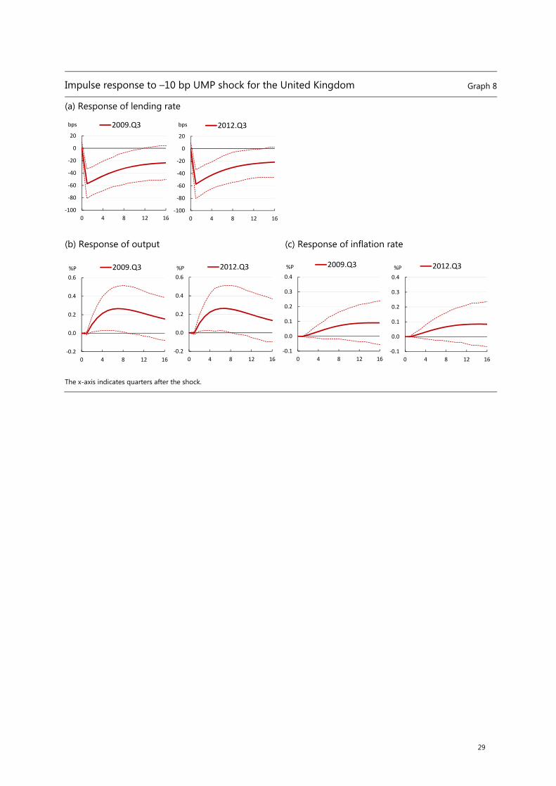
Graph 8(a) shows the impulse responses of the UK lending rate to a –10 bp UMP shock in Q3 2009 and Q3 2012. The 60 bp decline in the first quarter after the initial shock is similar at the two highlighted dates. While the depth of the impact looks large, at six times larger than the shock, it is consistent with the baseline model results. For the macroeconomic variables in Graphs 8(b) and (c), output growth and inflation respond positively to the UMP shock, which is consistent with studies by Kapitanios et al (2012), Weale and Wieladek (2016), and Haldane et al (2016). The key finding is quite similar responses of the macroeconomy across the selected times. In Q3 2012, the two-year yield was 0.2% and the 10-year yield 1.7%, which were close to historical lows in recent decades.
4.2. Declining interest rate sensitivity of the economy or declining effectiveness of monetary policy?
Our results raise the question of whether (A) the interest rate sensitivity of the economy was stable and the declining interest rates were offset by declines in the short-term “natural” rate of interest, or (B) the economy’s interest rate sensitivity declined but policy was less effective in a low interest rate environment. To assess the empirical relevance of these competing hypotheses, we let the data speak using the Bayesian posterior odds methods.
Bayesian posterior odds methods are well designed to answer this empirical question about these two hypotheses. One advantage of these methods is that we can compare both non-nested models in a statistical horse race. The posterior odds of the Model (A) over Model (B) are computed as
, = : ) : ) = : ) ( ): ) ( ) = ∏ ( | ) ( )∏ ( | ) ( ) where ∙ : ) is the posterior probability of the model, ( | ∙) is the marginal likelihood of the model and ( ∙) is the prior model probability. We compute the odds for the period after the GFC.
We use our TVP-VAR model to characterise each hypothesis. For hypothesis (A), we let the “natural” rate vary over time; this is captured with a TVP-VAR model using a time-varying “natural” rate of interest calibrated to match the HP-filtered

11
lending rate series.21 For hypothesis (B), we fix the level of the “natural” rate at the start of the crisis.
The posterior odds are striking: 23.9 for the United States; 15.8 for the euro area; 36.4 for Japan; and 10.9 for the United Kingdom. This result indicates that our cross-country data statistically support hypothesis (A) over (B), ie the data support the view that the economy did not become less interest sensitive during the GFC, but rather that monetary policy became less effective because of the decline in the “natural” rate. The interpretation of and possible explanations for this finding are discussed in Section 5.
4.3. Robustness
The estimation results in the analysis with the lending rate to non-financial corporations are fairly similar across countries, indicating that the effectiveness of the UMP on the macroeconomy did not appear to diminish in the low interest rate environment. Robustness tests with respect to the choice of the lending rate, prior parameter sensitivity and frequency of the unconventional monetary policy shocks confirm our findings. The following subsections describe our findings.
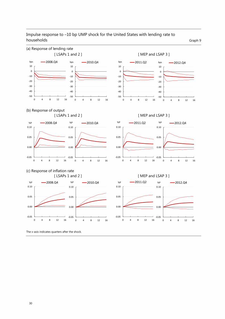
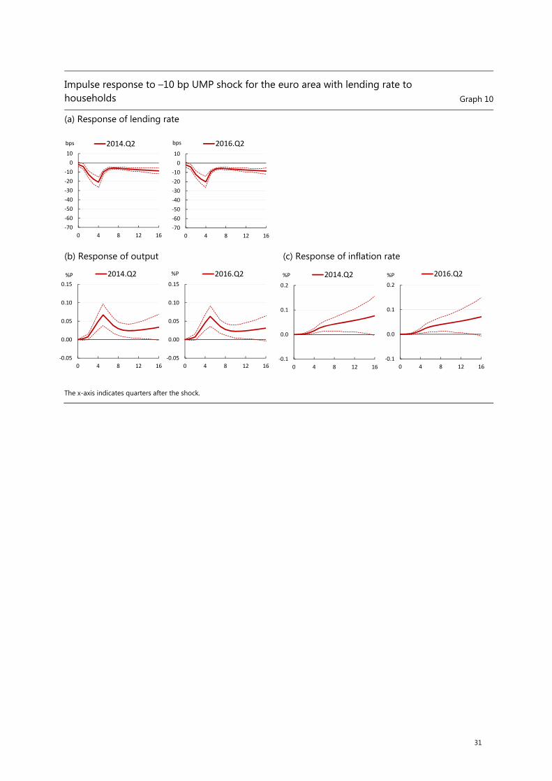
4.3.1. Using lending rates for households
Lending rates to non-financial corporation and households are highly correlated but may nonetheless evolve differently in response to UMP shocks. We use mortgage rates for the euro area and the United Kingdom. For the United States, we calculate an implied lending rate to households by dividing household debt service payments by the total amount of household debt. Real GDP growth is used instead of the quarterly growth in industrial production. Lacking a long time series of mortgage rates for Japan, we exclude Japan from this robustness check.
Graphs 9–11 display the estimated impulse responses of the household lending rates and of the macroeconomic variables to UMP shocks. The lending rates significantly decline in all countries, which implies a significant interest rate pass-through of UMP shocks to household lending rates. For the macroeconomic variables, confidence intervals of the impulse response are larger than those in the analysis with corporate lending rates. Despite these differences, UMP effectiveness does not appear to diminish over time.
4.3.2. Sensitivity of results to alternative prior hyperparameters
TVP-VAR model results can be sensitive to the choice of the prior hyperparameters that govern the variances of random-walk process. To assess this possibility, we estimate the model for all combinations of the hyperparameters, ∈ {0.01, 0.05, 0.1}, ∈ {0.1, 1}, and ∈ {1, 10}. Despite a modest decline in the mean estimate of the impulse response from the lending rate to the macroeconomic variables for some of the combinations, the qualitative findings do not fundamentally change.
21 Alternative specifications for the “natural” rate process that account for future parameter variation,
and hence feedbacks through an expectations channel, could improve the fit (see eg Johannsen and Mertens (2016)).
12
4.3.3. Higher-frequency data to identify the UMP shock
One can argue that such UMP shocks obtained from daily data may be noisy measures of the policy action. To address this concern, we rerun the US analysis using high-frequency, intra-day financial data to identify a monetary policy shock. In particular, we use the unconventional monetary policy shocks constructed by Ferrari et al (2017): the difference between the average sovereign bond yields 20 to five minutes before the announcement and the average five to 20 minutes after the announcement, for the same set of US UMP announcement dates. The overall picture is unaltered.
4.3.4. Using shadow rates
Related to the previous robustness check, one caveat in our approach is the limited number of non-zero UMP shocks in our data set. An alternative approach to identify the UMP shocks during the effective lower bound period is the use of shadow rates instead of the short-term policy rate. We employ the shadow rates estimated by Wu and Xia (2016, 2017) in our data set for the United States and the euro area, and rerun the TVP-VAR model where the UMP shock is identified based on the standard lower-triangular Choleski decomposition. Estimated impulse responses to the UMP shock show a smaller impact on the lending rate, output and inflation rate compared with our baseline UMP shocks, probably because the shadow rate captures not only the UMP shock but also various factors in financial market. Despite this difference, it is noteworthy that the impulse responses do not diminish over time.
5. Discussion
Focusing on the lending rate links in the monetary transmission mechanism sheds new light on the transmission mechanism of UMPs. Our findings place greater prominence on the pass-through of UMPs to lending rates than on shadow rates. Lending rates arguably play a more important role because these rates are the ones seen by the private sector. As such, they determine private sector incentives and hence outcomes.22
Our baseline model (ie a constant parameter VAR model) indicates a delayed pass-through from sovereign yields to lending rates, suggesting a lagged economic impact. In Graph 2, the lending rate impulse responses rise gradually compared to the more rapid responses of sovereign yields to UMP shocks: the gap between the lending rate and two-year yield widens on impact of the UMP shock, ie the two-year sovereign yield initially falls by nearly 30 bp but lending rates only fall 10 bp. After two quarters, the lending rate catches up with the sovereign yields and then both move in tandem.
In the TVP-VAR model, we find a similar hump-shaped response of lending rates. In contrast to the baseline model, the TVP-VAR does not impose quick mean reversion of the rates and yields to their respective unconditional means. This more flexible model captures the very persistent impact of UMP shocks on yields and rates.
22 In a different context, Blinder (1999) emphasised that monetary policy works by influencing the
interest rates and asset prices that matter to private decision-makers, ie lending rates and equity prices, for example. This is not to dismiss the importance of the link between UMPs and sovereign yields, but the pass-through to private sector lending rates is, in a sense, even more important owing to the fact that sovereign yields and bank lending rates do not appear to move in lock-step.

13
In Graph 3, an initial 10 bp shock to the lending rate is associated with a systematic, semi-permanent reduction in the lending rate of roughly the same size. Statistically, this effect is captured with the time-varying intercept in the lending rate equation. We interpret this as a very persistent decline in the lending rate as being consistent with previous studies which labeled the very persistent decline in the interest rate as evidence of a decline in the natural rate (ie in the absence of further shocks, the level to which the rate would gravitate over the medium term).23
Our evidence of a “natural” rate decline in response to a UMP shock deserves some explanation.24 In theory, time variation in the natural rate can reflect a number of real factors. For example, an exogenous increase in private sector domestic demand or a more expansionary fiscal policy would increase the natural rate.25 In other words, in theory, the natural rate moves around over time. A more fundamental question is whether it would be expected to change in response to a UMP shock. While there is nothing ruling out time-variation in the natural rate, theory suggests that the natural rate does not shift in response to monetary policy shocks.
If so, then an important question arises: what economic phenomenon might we be capturing? There are at least two possible explanations which could help to account for the correlation between the “natural” rate and UMP shocks in our sample; they are not mutually exclusive. The first is an “information” story along the lines of Morris and Shin (2002). In a time of extreme uncertainty about the economy, the private sector may naturally put considerable weight on a central bank’s assessment of the “natural” rate. In the case of persistently low inflation despite cuts in the policy rate, the central bank may conjecture that the natural rate had fallen. However, the central bank may not have an accurate estimate of the natural rate and simply communicate its best guess. In a self-reinforcing way, the private sector and the central bank may then convince themselves that this best guess is an unbiased estimate of the natural rate even when it is not. This dynamic might be particular relevant when a central bank intensifies its UMP efforts after receiving the corroborating market feedback. Of course, if the central bank is not in possession of more accurate information about the natural rate than the private sector, the information inferred by markets could prove unreliable and distorting.
The second explanation is a “scarce safe asset” story along the lines of Caballero et al (2016). The safe asset mechanism may help to explain a decline in the short-term “natural” rate at the time of UMP shocks. An increase in large-scale asset purchases removes safe assets from the marketplace.26 In this case, the premium on
23 One possibility is that the intercept reflects a permanent reduction in the term premia and not just
the expected steady state interest rate. The use of the two-year yield when defining the monetary policy shocks mitigates this misdiagnosis risk. Recent research has also been consistent with the notion that UMPs have had a larger impact on expected future interest rates than on the term premium.
24 It is an open question whether the monetary policy can affect the natural rate of interest. Laubach and Williams (2003), for example, assume that the natural rate is driven by the real economy. They do not include a role for signalling or a scarce asset friction in their model.
25 For discussions of the conventional determinants of time-variation in the natural rate, see Woodford (2003), Barsky et al (2014) and Holston et al (2017). Note also that Hakkio and Smith (2017) argue that, all else the same, UMPs resulting in a reduction in term premia should increase the natural rate. This mechanism may be at work but is inconsistent with the overall empirical results from our model.
26 In some respects the conventional safe asset story is incomplete. Taking account of how central banks implement monetary policy, the purchase of safe assets from the public results in the swapping of safe sovereign assets for safe reserves (ie assets) of the central bank. However, assuming banks cannot write safe securities pledged against these reserves, the general safe asset result holds.
14
safe assets would rise and the sovereign yields would decline in a very persistent fashion, assuming that the central bank balance sheet is expected to remain bloated for an extended period of time.27 This explanation finds some support from recent research showing that financial market real rates have diverged significantly from real returns on the aggregate capital stock (also see Marx et al (2017)); such a divergence suggests that central bank UMPs can distort financial market prices and expectations in a way disconnected from physical returns on capital.
Other possible explanations of this UMP-”natural” rate co-movement would contradict our findings. For example, if stimulative UMPs reduced the financing costs of the government, governments would have more room for manoeuver to increase fiscal stimulus. This would tend to increase the natural rate, not reduce it. Likewise, if the implied commitment of the central bank to “low for long” were to spark enthusiasm (eg animal spirits) and hence brighten prospects for a robust recovery, the “natural” rate would tend to rise.28
Regardless of the explanation, a lower perceived “natural” rate has implications for the stimulative power of UMPs. A reduction in the perceived “natural” rate would reduce the impact of UMPs, all else the same. Why? Consider a standard first-order condition of a standard representative consumer’s problem. If the interest rate faced by economic agents were to move in tandem with the perceived “natural”, or steady state, rate, the consumption path would remain relatively unchanged. In other words, the stimulative impact of monetary policy depends on the gap between the market rates faced by the private sector and the (perceived) “natural” rate (Graph 12, left-hand panel). The positive co-movement of policy interest rates and the “natural” rate blunts the effectiveness of monetary policy.29
What do these findings imply for the normalisation of central bank balance sheets? Central bank balance sheet normalisation is expected to go hand-in-hand with an increase in sovereign yields and lending rates. Under the information and safe asset explanations, the “natural” rate would retrace its path during a normalisation and therefore sap the strength of the policy rate rise.
Graph 12 (right-hand panel) illustrates the difference in the policy implications between the conventional approach and ours. The conventional approach implies a roughly unchanged path for the estimated “natural” rate, denoted by the light blue dashed line.30 Our findings imply a rising path, implied by the dark
27 Williamson (2017) notes that, in a neo-Fisherian model of monetary policy with collateral constraints
of the type of Caballero et al (2016), the purchase of government bonds lowers the real rate permanently as the collateral constraint tightens. Also see Uribe (2017) for further implications of neo-Fisherian monetary policy dynamics. He argues that “interest-rate increases that are perceived to be permanent cause a temporary decline in real rates with inflation adjusting faster than the nominal interest rate to a higher permanent level”, implying a rapid increase in inflation to target without adverse consequences for aggregate activity.
28 Note also that Hakkio and Smith (2017) argue that, all else the same, UMPs resulting in a reduction in term premia should increase the natural rate. This mechanism may be at work but is inconsistent with the overall empirical results from our model.
29 Highly accommodative monetary policy (via very low policy rates and large-scale asset purchase programmes) can led to a gradual decline in the natural rate that would not be picked up with our empirical exercise. The decline is thought to result from hysteresis of various types. Recent research has focused on the implications of zombie firms. See eg Adalet McGowan et al (2017), Caballero et al (2008), Forbes (2015) and Obstfeld and Duval (2018) for a discussion of low interest rate environments and zombie firms.
30 Conventional models (eg Laubach and Williams (2003)) typically characterise the natural rate as random walk, ie the best forecast of the “natural” rate estimate is today’s estimate.
15
blue dotted line. This difference raises the possibility that a tight stance relative to the conventionally estimated benchmark would represent a continuation of the very accommodative policy relative to the path implied by our findings. In this case, underestimating the size of the “natural” rate reversal could result in central banks finding themselves unwittingly falling behind the curve.
Two notes of caution should be kept in mind. First, some might question the reliability of the correlations in the paper due to the unprecedented nature of the monetary policy environment. True, monetary authorities are navigating in an unprecedented nominal policy environment. Nominal policy rates have never been so persistently low. But low real interest rates have remained well within the range of historical experience. For illustrative purposes, Graph 13 shows the real rate gaps for the United States and Canada. The current level of the real rate gap for both countries has gravitated toward the lower edge of the grey band since 1990. If we evaluate the series back to the 1960s, the current level of the real rate gap is well within the one-standard-deviation band shown in the graph. Thus, in terms of capturing the monetary transmission mechanism, the real interest rate environment does not look extreme, suggesting that our empirical design may not suffer from acute biases vis-à-vis conventional Lucas critique concerns.
Second, the implications of central bank balance sheet normalisation mentioned above are based on the assumption of symmetry – that is, the impacts in the build-up will reverse in the normalisation. However, recent announcements from the Federal Reserve indicate an intention to de-link the rate normalisation from the balance sheet normalisation. During the balance sheet build-up, the two policy tools were closely linked. The ability to de-link the policy tools in the normalisation is more likely if the original UMP impacts were largely of a signalling nature. If the link was through the portfolio rebalancing channel, the ability to de-link the policy tools would be more difficult.
6. Concluding remarks
We find that unconventional monetary policies were effective in providing some stimulus to economies at the perceived lower bound for policy rates. The responsiveness of the economy to private sector interest rates remained remarkably stable in our sample. However, it must also be noted that the overall effectiveness fell for two key reasons. First, the “bang for the buck” of central bank balance sheet stimulus declined over time. Larger and larger programmes were necessary to achieve a given change in sovereign yields. Second, the “natural” rate tended to decline with (unexpected) expansionary unconventional monetary policies. This suggests that monetary policy decisions have influenced the perceived “natural” rate, contrary to what is implied by the conventional wisdom. This correlation may also help to explain why monetary policy appears to have had been less stimulative than expected in the past decade, and may indicate that monetary policy could prove to be more stimulative than expected during the normalisation with no change in the conventional wisdom.
This study highlights the importance of a better understanding of the mechanisms at work. Such knowledge could help in assessing the future use of central bank balance sheet tools. Of course, their attractiveness also depends on the costs they impose on the economy. A reliance on balance sheet tools can, for example, result in resource misallocations, disruptive risk-taking behaviour and political

16
economy challenges. These costs, among others, would have to be weighed against the benefits when considering the appropriate role for central bank balance sheets in the new normal era as well as in future crisis periods.
Having said this, various caveats should be highlighted. The empirical results in the paper admittedly have to be interpreted with particular care. The data sample is relatively short, making it difficult to draw definitive inferences about the effectiveness of unconventional monetary policies on the macroeconomy. And, as is typically the case, time-varying models tend to be less accurate at the end of samples. All this suggests that we need to be careful when evaluating the macro evidence and we need to corroborate any findings with the micro evidence. In addition, some unique features of the new regulatory and monetary policy environment may raise questions about how far the policies implemented in the past decade can continue to be as effective in the future. Such issues are left for future research.
17
Appendix 1 Data description
This appendix describes the choice of the variables used in our model: core CPI inflation ( ), output growth ( ), short-term policy interest rate ( ), the exchange rate ( ), the lending rate (ℓ ) and the UMP shock ( ).
A.1.1. United States
: CPI for all items less food and energy, year-on-year rate of change. : total industrial production excluding construction, seasonally adjusted, quarter-on-quarter change; or real GDP, quarterly growth rate. : effective federal funds rate. ℓ : Commercial and Industrial (C&I) loan rates for all commercial banks from the Federal Reserve Survey of Terms of Business Lending. This survey estimates the terms of loans extended during the first full business week in the middle month of each quarter. For the robustness check, the 30-year fixed mortgage rate is used.
: the UMP shocks cover a series of large-scale asset purchase programs (LSAP 1 to 3) starting in Q4 2008 and the maturity extension program (MEP). We divide these policies to the following two periods: (1) the LSAP1 and LSAP2 and (2) MEP and LSAP3; and assign the monetary policy shocks of policy announcements to
and . The last non-zero observation in is Q4 2012. The estimation period spans from Q3 1986 to Q2 2016. The effective lower bound restriction is imposed once the federal funds rate range hit zero to 25 bp.
A.1.2. United Kingdom
: CPI all items index, year-on-year rate of change. Because the core CPI available for shorter periods, the headline CPI is used for the United Kingdom. : industrial production for all industry excluding construction, seasonally adjusted, quarter-on-quarter change; or real GDP, quarterly growth rate. : official bank rate. ℓ : the weighted average interest rate on other loans and new advances to private non-financial firms and the mortgage rate, obtained from Bank of England. : the UMP shocks cover the first and second quantitative easing programmes starting in Q1 2009 with the last policy announcement in Q3 2012. The estimation period spans from Q1 1983 to Q2 2016. The effective lower bound restriction is imposed once the bank rate hit 50 bp.
A.1.3. Euro area
: HICP for all items excluding energy and food, year-on-year rate of change. : total industrial production excluding construction, seasonally adjusted, quarter-on-quarter change; or real GDP, quarterly growth rate. : the Euro Overnight Index Average (EONIA). Before 1999, the German money-market overnight interest rate is used. ℓ : interest rates on loans to non-financial corporations with a floating rate and an initial period of fixation of the interest rate (IRF) period of over five years, obtained from the MFI Interest Rate Statistics. Before 1999, the German bank discount rate of commercial bills is used. For the robustness check, interest rates on loans to households for house purchase with a floating rate and an IRF period over one year is used. We take weighted average of the rates across the countries by the PPP value of GDP.
18
: the UMP shocks cover a series of asset purchase programmes (APPs) from Q2 2009. The last observation of policy announcements in our sample is in Q1 2016. The estimation period spans from Q1 1995 to Q2 2016. The effective lower bound restriction is imposed once the deposit facility rate hit zero.
A.1.4. Japan
: CPI excluding fresh food, adjusted to remove the effect of the increase in the consumption tax. : industrial production, seasonally adjusted, quarter-on-quarter change; or real GDP, quarterly growth rate. : overnight call rate, ℓ : long-term prime lending rates, obtained from the Bank of Japan. Because this is the reference rate, another lending rate, average contract interest rates on loans and discounts are better alternative in line with the lending rates for other countries in our analysis. However, because the latter rates are only available for shorter periods, we use the former rates. :the Bank of Japan implemented a series of UMPs from 2001, which is divided into the following four periods in our analysis. (1) the first quantitative easing policy from Q1 2001 to Q2 2006; (2) the fund-supplying operation (a fixed-rate funds-supplying operation against pooled collateral) from Q4 2009 to Q3 2010; (3) the comprehensive monetary easing (CME) policy from Q4 2010 to Q1 2013; (4) the quantitative and qualitative monetary easing (QQE) policy from Q2 2013. We assign the monetary policy shocks of policy announcement during each period to , for = 1,… , 4. The last observation of policy announcements in is Q1 2016. The estimation period spans from Q1 1984 to Q2 2016. The effective lower bound restriction is imposed once the overnight call/deposit rate is equal or below 25 bp.
A.1.5. Exchange rates
The real exchange rate is constructed with the nominal exchange rate, and domestic and foreign price indices. For economies other than the United States, we use the nominal exchange rate against the US dollar, domestic and US headline CPI. For the United States, we construct a trade-weighted index for the foreign variables. We select the first six largest trading partners of the United States by their export volumes and take weighted averages of USD-cross nominal exchange rates and headline CPIs of those economies. Regarding the domestic and foreign interest rates, and ∗, we use three-month interest rates to match their maturity with the quarter-on-quarter change in the exchange rate in the left hand side of regression. We construct the trade-weighted interest rates as the foreign interest rate for the United States in the same manner as the real exchange rate above.
We compute the exchange rate variable used in our VAR analysis, by regressing the interest rate differentials on a change in the real exchange rate denoted by ∆ : ∆ = + ( − ∗) + , where and ∗ are domestic and foreign interest rates, respectively. The resulting estimated residual denoted by is the change in the nominal exchange rate that is orthogonal to changes in domestic and foreign interest rates, which we use as the exchange rate variable, namely, = .31
31 This choice reflects the empirical properties of exchange rates found in various papers (eg Engel
(1996), Jordà and Taylor (2012) and Boudoukh et al (2016)).
19
References
Adalet McGowan, M, D Andrews and V Millot (2017): “The walking dead?: zombie firms and productivity performance in OECD countries”, OECD Economics Department Working Papers, no 1372.
Adrian, T and H S Shin (2011): “Financial intermediary balance sheet management”, Annual Review of Financial Economics, vol 3, no 1, pp 289−307.
Albertazzi, U, A Nobili and F Signoretti (2016): “The bank lending channel of conventional and unconventional monetary policy”, Bank of Italy Working Papers, no 1094.
Al-Dejaily, M, J Murphy and A Tibrewal (2012): “Distribution of balances from effective interest rate data”, Bank of England Monetary and Financial Statistics.
Altavilla, C, F Canova and M Ciccarelli (2016a): “Mending the broken link: heterogeneous bank lending and monetary policy pass-through”, CEPR Discussion Papers, no DP11584.
Altavilla, C, D Giannone and M Lenza (2016b): “The financial and macroeconomic effects of OMT announcements”, International Journal of Central Banking, vol 12, no 3, pp 29−57.
Bank for International Settlements (2016): 86th Annual Report, June.
Bank of Japan (2016): “Comprehensive assessment: developments in economic activity and prices as well as policy effects since the introduction of quantitative and qualitative monetary easing (QQE): the background”, September 2016.
Barsky, R, A Justiniano and L Melosi (2014): “The natural rate of interest and its usefulness for monetary policy,” American Economic Review: Papers & Proceedings, vol 104, no 5, pp 37–43.
Baumeister, C and L Benati (2013): “Unconventional monetary policy and the great recession: estimating the macroeconomic effects of a spread compression at the zero lower bound”, International Journal of Central Banking, vol 9, no 2, pp 165−212.
Baumeister, C and G Peersman (2013): “Time-varying effects of oil supply shocks on the US economy”, American Economic Journal: Macroeconomics, vol 5, no 4, pp 1−28.
Bech, M, L Gambacorta and E Kharroubi (2014): “Monetary policy in a downturn: are financial crises special?”, International Finance, vol 17, no 1, pp 99−119.
Bernanke, B and K Kuttner (2005): “What explains the stock market’s reaction to Federal Reserve policy?”, Journal of Finance, vol 60, no 3, pp 1221−57.
Blinder, A (1999): Central banking in theory and practice, MIT Press.
Borio, C, L Gambacorta and B Hofmann (2015): “The influence of monetary policy on bank profitability”, BIS Working Papers, no 514.
Borio, C and A Zabai (2016): “Unconventional monetary policies: a re-appraisal”, BIS Working Papers, no 570.
Boudoukh, J, M Richardson and R Whitelaw (2016): “New evidence on the forward premium puzzle”, Journal of Financial and Quantitative Analysis, vol 51, no 3, pp 875−97.
Caballero, R, E Farhi and P-O Gourinchas (2016): “Safe asset scarcity and aggregate demand”, American Economic Review, vol 106, no 5, pp 513−8.
20
Caballero, R, T Hoshi and A Kashyap (2008): “Zombie lending and depressed restructuring in Japan”, American Economic Review, vol 98, no 5, pp 1943−77.
Chen, H, V Cúrdia and A Ferrero (2012): “The macroeconomic effects of large-scale asset purchase programmes”, Economic Journal, vol 122, no 564, pp F289−F315.
Chen, Q, A Filardo, D He and F Zhu (2016): “Financial crisis, US unconventional monetary policy and international spillovers”, Journal of International Money and Finance, vol 67, pp 62−81.
——— (2017): “Domestic and cross-border impact of US monetary policy at the zero lower bound”, forthcoming.
Cheng, C and C Chiu (2016): “Nonlinearities of mortgage spreads over the business cycles”, Bank of England Staff Working Paper, no 634.
Dahlhaus, T (2014): “Monetary policy transmission during financial crises: an empirical analysis”, Bank of Canada Working Papers, no 2014-12.
Engel, C (1996): “The forward discount anomaly and the risk premium: a survey of recent evidence”, Journal of Empirical Finance, vol 3, no 2, pp 123−92.
European Central Bank (2017): “MFI lending rates: pass-through in the time of non-standard monetary policy”, Economic Bulletin, Article 1, January.
European Insurance and Occupational Pensions Authority (2014): Low interest rate environment stock taking exercise 2014, EIOPA-BoS-14/103.
Ferrari, M, J Kearns and A Schrimpf (2015): “Monetary policy’s rising FX impact in the era of ultra-low rates”, BIS Working Papers, no 626.
Forbes, K (2015): “Low interest rates: King Midas’ golden touch?”, speech at the Institute of Economic Affairs, London, 24 February.
Gagnon, J, M Raskin, J Remache and B Sack (2011): “The financial market effects of the Federal Reserve’s large-scale asset purchases”, International Journal of Central Banking, vol 7, no 1, pp 3−43.
Gambacorta, L, B Hofmann and G Peersman (2014): “The effectiveness of unconventional monetary policy at the zero lower bound: a cross-country analysis”, Journal of Money, Credit and Banking, vol 46, no 4, pp 615−42.
Gambacorta, L, A Illes and M Lombardi (2014): “Has the transmission of policy rates to lending rates been impaired by the Global Financial Crisis?”, BIS Working Papers, no 477.
Gertler, M and P Karadi (2015): “Monetary policy surprises, credit costs, and economic activity”, American Economic Journal: Macroeconomics, vol 7, no 1, pp 44−76.
Giannone, D, M Lenza and L Reichlin (2008): “Explaining the great moderation: it is not the shocks”, Journal of the European Economic Association, vol 6, no 2-3, pp 621−33.
Hakkio, C and A Smith (2017): “Bond premiums and the natural real rate of interest”, Economic Review, Federal Reserve Bank of Kansas City, first quarter, pp 5–40.
Haldane, A, M Roberts-Sklar, C Young and T Wieladek (2016): “QE: the story so far”, Bank of England Staff Working Paper, no 624.
Hesse, H, B Hofmann and J Weber (2017): “The macroeconomic effects of asset purchases revisited”, BIS Working Papers, forthcoming.

21
Hofer, H, K Schlepper, A Schrimpf and R Riordan (2017): “Scarcity effects of QE: A transaction-level analysis in the Bund market”, unpublished BIS Working Paper, January.
Holston, K, T Laubach and J Williams (2017): “Measuring the natural rate of interest: international trends and determinants”, Journal of International Economics, forthcoming.
Illes, A, M Lombardi and P Mizen (2015): “Why did bank lending rates diverge from policy rates after the financial crisis?”, BIS Working Papers, no 486.
Iwasaki, Y and N Sudo (2017): “Myths and observations on unconventional monetary policy: takeaways from post-bubble Japan”, Bank of Japan Working Paper Series, no 17-E-11.
Johannsen, B and E Mertens (2016): “A time series model of interest rates with the effective lower bound”, FEDS Working Paper, no 2016-033.
Jordà, Ò and A Taylor (2012): “The carry trade and fundamentals: nothing to fear but FEER itself”, Journal of International Economics, vol 88, no 1, pp 74−90.
Kapetanios, G, H Mumtaz, I Stevens and K Theodoridis (2012): “Assessing the economy-wide effects of quantitative easing”, Economic Journal, vol 122, no 564, pp F316−F347.
Kimura, T and J Nakajima (2016): “Identifying conventional and unconventional monetary policy shocks: A latent threshold approach”, B.E. Journal of Macroeconomics, vol 16, no 1, pp 277−300.
Koop, G, R Leon-Gonzalez and R Strachan (2009): “On the evolution of the monetary policy transmission mechanism”, Journal of Economic Dynamics and Control, vol 33, no 4, pp 997−1017.
Kuttner, K (2001): “Monetary policy surprises and interest rates: evidence from the Fed funds futures market”, Journal of Monetary Economics, vol 47, no 3, pp 523−44.
Laubach, T and J Williams (2003): “Measuring the natural rate of interest”, Review of Economics and Statistics, vol 85, no 4, pp 1063−70.
Lombardi, D and P Siklos (2017): “A survey of the international evidence and lessons learned about unconventional monetary policies: is a ‘new normal’ in our future?”, unpublished CIGI working paper, December.
Marx, M, B Mojon and F Velde (2017): “Why have interest rates fallen far below the return on capital”, Banque de France Working Paper, no 630, May.
Morris, S and H Shin (2002): “The social value of public information,” American Economic Review, vol 92, pp 1521−34.
Nakajima, J (2011): “Time-varying parameter VAR model with stochastic volatility: an overview of methodology and empirical applications”, Monetary and Economic Studies, vol 29, pp 107−42.
Obstfeld, M and R Duval (2018): “Tight monetary policy is not the answer to weak productivity growth”, VoxEU, 10 January.
Panizza, U and C Wyplosz (2016): “The folk theorem of decreasing effectiveness of monetary policy: what do the data say?”, prepared for the IMF 17th Jacques Polak Annual Research Conference.
22
Peersman, G (2011): “Macroeconomic effects of unconventional monetary policy in the euro area”, CEPR Discussion Paper, no 8348.
Primiceri, G (2005): “Time varying structural vector autoregressions and monetary policy”, Review of Economic Studies, vol 72, no 3, pp 821−52.
Uribe, M (2017): “The neo-Fisher effect in the United States and Japan”, NBER Working Paper, no 23977, October.
von Borstel, J, S Eickmeier and L Krippner (2016): “The interest rate pass-through in the euro area during the sovereign debt crisis”, Journal of International Money and Finance, vol 68, pp 386−402.
Weale, M and T Wieladek (2016): “What are the macroeconomic effects of asset purchases?”, Journal of Monetary Economics, vol 79, pp 81−93.
Williamson, S (2017): “Low interest rates and the zero lower bound”, Federal Reserve Bank of St Louis Working Paper, no 2017-010A, April.
Woodford, M (2003): Interest and Prices: Foundations of a Theory of Monetary Policy, Princeton University Press.
Wu, J and F Xia (2016): “Measuring the macroeconomic impact of monetary policy at the zero lower bound”, Journal of Money, Credit and Banking, vol 48, no 2-3, pp 253−21.
——— (2017): “Time-varying lower bound of interest rates in Europe”, Chicago Booth Research Paper, no 17-06.
23
Bank lending rates to non-financial corporations Graph 1
United States Euro area
United Kingdom Japan
-1
0
1
2
3
4
5
95 00 05 10 15
%
0
2
4
6
8
10
95 00 05 10 15
%
-1
0
1
2
3
4
5
6
7
95 00 05 10 15
%
0
2
4
6
8
10
95 00 05 10 15
%
Lending rate 10-year yield 2-year yield Short-term interest rate
24
Impulse response of lending rate to –10 bp UMP shock Graph 2
United States Euro area
United Kingdom Japan
The x-axis indicates quarters after the shock. The red dotted lines indicate 68% confidence intervals for the response of the lending rate.
-50
-40
-30
-20
-10
0
10
20
0 4 8 12 16
bps
Lending rate 2-year yield 10-year yield
-60-50-40-30-20-10
0102030
0 4 8 12 16
bps
-80
-60
-40
-20
0
20
40
0 4 8 12 16
bps
-120
-80
-40
0
40
80
0 4 8 12 16
bps

25
-50
-40
-30
-20
-10
0
10
0 4 8 12 16
2011.Q2bps
-50
-40
-30
-20
-10
0
10
0 4 8 12 16
2012.Q4bps
Impulse response to –10 bp UMP shock for the United States Graph 3
(a) Response of lending rate [ LSAPs 1 and 2 ] [ MEP and LSAP 3 ]
(b) Response of output [ LSAPs 1 and 2 ] [ MEP and LSAP 3 ]
(c) Response of inflation rate [ LSAPs 1 and 2 ] [ MEP and LSAP 3 ] The x-axis indicates quarters after the shock.
-0.05
0.00
0.05
0.10
0.15
0 4 8 12 16
2011.Q2%P
-0.05
0.00
0.05
0.10
0.15
0 4 8 12 16
2012.Q4%P
-50
-40
-30
-20
-10
0
10
0 4 8 12 16
2008.Q4bps
-50
-40
-30
-20
-10
0
10
0 4 8 12 16
2010.Q4bps
-0.1
0.0
0.1
0.2
0.3
0 4 8 12 16
2008.Q4%P
-0.1
0.0
0.1
0.2
0.3
0 4 8 12 16
2010.Q4%P
-0.05
0.00
0.05
0.10
0.15
0 4 8 12 16
2008.Q4%P
-0.05
0.00
0.05
0.10
0.15
0 4 8 12 16
2010.Q4%P
-0.1
0.0
0.1
0.2
0.3
0 4 8 12 16
2011.Q2%P
-0.1
0.0
0.1
0.2
0.3
0 4 8 12 16
2012.Q4%P

26
Impulse response to –10 bp UMP shock for Japan Graph 4
(a) Response of lending rate [ CME ] [ QQE ]
(b) Response of output [ CME ] [ QQE ]
(c) Response of inflation rate [ CME ] [ QQE ] The x-axis indicates quarters after the shock.
-0.6-0.4-0.20.00.20.40.60.81.0
0 4 8 12 16
2013.Q2%P
-0.6-0.4-0.20.00.20.40.60.81.0
0 4 8 12 16
2016.Q2%P
-100
-80
-60
-40
-20
0
20
40
0 4 8 12 16
2013.Q2bps
-100
-80
-60
-40
-20
0
20
40
0 4 8 12 16
2016.Q2bps
-100
-80
-60
-40
-20
0
20
40
0 4 8 12 16
2010.Q4bps
-100
-80
-60
-40
-20
0
20
40
0 4 8 12 16
2012.Q4bps
-0.6-0.4-0.20.00.20.40.60.81.0
0 4 8 12 16
2010.Q4%P
-0.6-0.4-0.20.00.20.40.60.81.0
0 4 8 12 16
2012.Q4%P
-0.15
-0.10
-0.05
0.00
0.05
0.10
0.15
0 4 8 12 16
2010.Q4%P
-0.15
-0.10
-0.05
0.00
0.05
0.10
0.15
0 4 8 12 16
2012.Q4%P
-0.15
-0.10
-0.05
0.00
0.05
0.10
0.15
0 4 8 12 16
2013.Q2%P
-0.15
-0.10
-0.05
0.00
0.05
0.10
0.15
0 4 8 12 16
2016.Q2%P
27
Impulse response to –10 bp UMP shock for the Japan, counterfactual simulation Graph 5
(a) Response of output (b) Response of inflation rate
The x-axis indicates quarters after the shock.
-0.5
0.0
0.5
1.0
1.5
0 4 8 12 16
2016.Q2
1991.Q2
%P
-0.2
-0.1
0.0
0.1
0.2
0 4 8 12 16
2016.Q2
1991.Q2
%P
28
Impulse response to –10 bp UMP shock for the euro area Graph 6
(a) Response of lending rate
(b) Response of output (c) Response of inflation rate
The x-axis indicates quarters after the shock.
Impulse response to –10 bp UMP shock for the euro area, counterfactual simulation Graph 7
(a) Response of output (b) Response of inflation rate
The x-axis indicates quarters after the shock.
-70
-60
-50
-40
-30
-20
-10
0
0 4 8 12 16
2014.Q2bps
-70
-60
-50
-40
-30
-20
-10
0
0 4 8 12 16
2016.Q2bps
-0.05
0.00
0.05
0.10
0.15
0.20
0.25
0.30
0 4 8 12 16
2014.Q2%P
-0.05
0.00
0.05
0.10
0.15
0.20
0.25
0.30
0 4 8 12 16
2016.Q2%P
-0.05
0.00
0.05
0.10
0 4 8 12 16
2014.Q2%P
-0.05
0.00
0.05
0.10
0 4 8 12 16
2016.Q2%P
-0.1
0.0
0.1
0.2
0.3
0.4
0 4 8 12 16
2016.Q2
2007.Q2
%P
-0.05
0.00
0.05
0.10
0 4 8 12 16
2016.Q2
2007.Q2
%P
29
Impulse response to –10 bp UMP shock for the United Kingdom Graph 8
(a) Response of lending rate
(b) Response of output (c) Response of inflation rate
The x-axis indicates quarters after the shock.
-100
-80
-60
-40
-20
0
20
0 4 8 12 16
2009.Q3bps
-100
-80
-60
-40
-20
0
20
0 4 8 12 16
2012.Q3bps
-0.2
0.0
0.2
0.4
0.6
0 4 8 12 16
2009.Q3%P
-0.2
0.0
0.2
0.4
0.6
0 4 8 12 16
2012.Q3%P
-0.1
0.0
0.1
0.2
0.3
0.4
0 4 8 12 16
2009.Q3%P
-0.1
0.0
0.1
0.2
0.3
0.4
0 4 8 12 16
2012.Q3%P
30
Impulse response to –10 bp UMP shock for the United States with lending rate to households Graph 9
(a) Response of lending rate [ LSAPs 1 and 2 ] [ MEP and LSAP 3 ]
(b) Response of output [ LSAPs 1 and 2 ] [ MEP and LSAP 3 ]
(c) Response of inflation rate [ LSAPs 1 and 2 ] [ MEP and LSAP 3 ] The x-axis indicates quarters after the shock.
-50
-40
-30
-20
-10
0
10
0 4 8 12 16
2011.Q2bps
-50
-40
-30
-20
-10
0
10
0 4 8 12 16
2012.Q4bps
-50
-40
-30
-20
-10
0
10
0 4 8 12 16
2008.Q4bps
-50
-40
-30
-20
-10
0
10
0 4 8 12 16
2010.Q4bps
-0.05
0.00
0.05
0.10
0 4 8 12 16
2008.Q4%P
-0.05
0.00
0.05
0.10
0 4 8 12 16
2010.Q4%P
-0.05
0.00
0.05
0.10
0 4 8 12 16
2008.Q4%P
-0.05
0.00
0.05
0.10
0 4 8 12 16
2010.Q4%P
-0.05
0.00
0.05
0.10
0 4 8 12 16
2011.Q2%P
-0.05
0.00
0.05
0.10
0 4 8 12 16
2012.Q4%P
-0.05
0.00
0.05
0.10
0 4 8 12 16
2011.Q2%P
-0.05
0.00
0.05
0.10
0 4 8 12 16
2012.Q4%P
31
Impulse response to –10 bp UMP shock for the euro area with lending rate to households Graph 10
(a) Response of lending rate
(b) Response of output (c) Response of inflation rate
The x-axis indicates quarters after the shock.
-70-60-50-40-30-20-10
010
0 4 8 12 16
2014.Q2bps
-70-60-50-40-30-20-10
010
0 4 8 12 16
2016.Q2bps
-0.05
0.00
0.05
0.10
0.15
0 4 8 12 16
2014.Q2%P
-0.05
0.00
0.05
0.10
0.15
0 4 8 12 16
2016.Q2%P
-0.1
0.0
0.1
0.2
0 4 8 12 16
2014.Q2%P
-0.1
0.0
0.1
0.2
0 4 8 12 16
2016.Q2%P

32
Impulse response to –10 bp UMP shock for the United Kingdom with lending rate to households Graph 11
(a) Response of lending rate
(b) Response of output (c) Response of inflation rate
The x-axis indicates quarters after the shock.
-100
-80
-60
-40
-20
0
20
0 4 8 12 16
2009.Q3bps
-100
-80
-60
-40
-20
0
20
0 4 8 12 16
2012.Q3bps
-0.2
0.0
0.2
0.4
0.6
0 4 8 12 16
2009.Q3%P
-0.2
0.0
0.2
0.4
0.6
0 4 8 12 16
2012.Q3%P
-0.1
0.0
0.1
0.2
0.3
0.4
0 4 8 12 16
2009.Q3%P
-0.1
0.0
0.1
0.2
0.3
0.4
0 4 8 12 16
2012.Q3%P
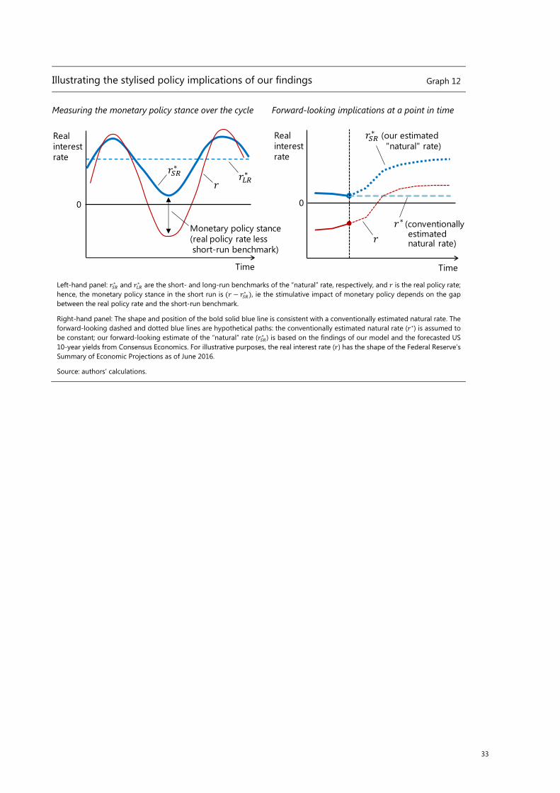
33
Illustrating the stylised policy implications of our findings Graph 12
Measuring the monetary policy stance over the cycle Forward-looking implications at a point in time
Left-hand panel: ∗ and ∗ are the short- and long-run benchmarks of the “natural” rate, respectively, and is the real policy rate; hence, the monetary policy stance in the short run is ( − ∗ ), ie the stimulative impact of monetary policy depends on the gap between the real policy rate and the short-run benchmark.
Right-hand panel: The shape and position of the bold solid blue line is consistent with a conventionally estimated natural rate. The forward-looking dashed and dotted blue lines are hypothetical paths: the conventionally estimated natural rate ( ∗) is assumed to be constant; our forward-looking estimate of the “natural” rate ( ∗ ) is based on the findings of our model and the forecasted US 10-year yields from Consensus Economics. For illustrative purposes, the real interest rate ( ) has the shape of the Federal Reserve’s Summary of Economic Projections as of June 2016.
Source: authors’ calculations.
∗ (our estimated
∗ (conventionallyestimated
"natural" rate)
Time
0
natural rate)
∗∗
Monetary policy stance(real policy rate lessshort-run benchmark)
0
Time
Realinterestrate
Realinterestrate

34
Real rate gap Graph 13
(a) United States (b) Canada
The shadow area indicates ±1 standard deviation from the historical mean of the time series. For the natural rate of interest, we use estimates by Holston et al (2017).
-8
-6
-4
-2
0
2
4
6
8
1960 65 70 75 80 85 90 95 2000 05 10 15
%
-10-8-6-4-202468
1960 65 70 75 80 85 90 95 2000 05 10 15
%
Previous volumes in this series
No Title Author
690 January 2018
Nonlinear State and Shock Dependence of Exchange Rate Pass-through on Prices
Hernán Rincón-Castro and Norberto Rodríguez-Niño
689 January 2018
Estimating unknown arbitrage costs: evidence from a three-regime threshold vector error correction model
Kristyna Ters and Jörg Urban
688 January 2018
Global Factors and Trend Inflation Gunes Kamber and Benjamin Wong
687 January 2018
Searching for Yield Abroad: Risk-Taking through Foreign Investment in U.S. Bonds
John Ammer, Stijn Claessens, Alexandra Tabova and Caleb Wroblewski
686 January 2018
Determinants of bank profitability in emerging markets
Emanuel Kohlscheen, Andrés Murcia Pabón and Julieta Contreras
685 December 2017
Why so low for so long? A long-term view of real interest rates
Claudio Borio, Piti Disyatat, Mikael Juselius and Phurichai Rungcharoenkitkul
684 December 2017
Triffin: dilemma or myth? Michael D Bordo and Robert N McCauley
683 December 2017
Can macroprudential measures make crossborder lending more resilient?
Előd Takáts and Judit Temesvary
682 December 2017
Bank business models: popularity and performance
Rungporn Roengpitya, Nikola Tarashev, Kostas Tsatsaronis and Alan Villegas
681 December 2017
Corporate leverage in EMEs: Did the global financial crisis change the determinants?
Snehal S Herwadkar
680 December 2017
The Macroeconomic Effects of Asset Purchases Revisited
Henning Hesse, Boris Hofmann and James Weber
679 December 2017
Syndicated loans and CDS positioning Iñaki Aldasoro and Andreas Barth
All volumes are available on our website www.bis.org.