bits wase computergraphics session 13 14

Session 13 and 14Visible Surface Detection Algorithms:

Object Space Based, Image Space Based and List Priority Based : Chapter 15

Course Delivery by

Dr. K. Satyanarayan Reddy

Text Book

Computer Graphics: Principles and Practice in C, 2nd edition Pearson Education.

By James D. Foley, A. Van Dam, S.K. Feiner, and J.F. Hughes

Visible Surface DeterminationVisible Line or Visible Surface Determination: Given a set of 3D

objects and a viewing specification, then to determine which lines or

surfaces of the objects are visible, either from the center of

projection (for perspective projections) or along the direction of

projection (for parallel projections), so that only the visible lines or

surfaces can be displayed.

This process is known as Visible Line or Visible Surface

determination, or HIDDEN-LINE or Hidden-Surface Elimination.

ln Visible Line Determination, the lines are assumed to be the edges of

opaque surfaces that may obscure the edges of other surfaces farther

from the viewer.

In general, this process is referred to as the Visible Surface

Determination.

February 1, 2014 BITS WASE Computer Graphics: Course Delivery By Dr. K. Satyanarayan Reddy 2

The first approach determines which of n objects is visible at each pixel in the image.

The pseudocode for this approach looks like this;

for (each pixel in the image)

{

determine the object closest to the viewer i.e. pierced by the projectorthrough the pixel;

draw the pixel in the appropriate color;

}

The second approach is to compare objects directly with each other, eliminating entireobjects or portions of them that are not visible.

Expressed in pseudocode, this becomes

for (each object in the world)

{

determine those parts of the object whose view is unobstructed

by other parts of it or any other object;

draw those parts in the appropriate color;

}


Visible Surface Determination cont’d….

FUNCTIONS OF TWO VARIABLES One of the most common uses of computer graphics is to plot Single

Valued continuous functions of two variables, such as

y = f(x, z).

These functions define surfaces like that shown in Fig. l5.l(a). They

present an interesting special case of the Hidden Surface Problem,

for which especially fast solutions are possible.


Consider the ‘ ‘silhouette boundary" of the polylines drawn thus far on the view plane,

shown as thick lines in Fig. 15.2. When a new polyline is drawn, it should be

visible only where its projection rises above the top or dips below the bottom of

the old silhouette.

Since each new polyline has a constant z that is farther than that of any of the

preceding polylines, it cannot pierce any part of the surface already drawn.

Therefore, to determine what parts are to be drawn, the current polyline’s projected y

values need only to be compared with those of the corresponding part of the

surface’s silhouette computed thus far.

When only enough information is encoded to represent a minimum and maximum

silhouette y for each x, the algorithm is known as an horizon line algorithm.


FUNCTIONS OF TWO VARIABLES cont’d….

One way to represent this silhouette, implemented by Wright, uses two ID arrays, YMIN and YMAX, to hold the minimum

and maximum projected y values for a finite set of projected x values.

These are image-precision data structures because they have a finite number of entries.

YMIN and YMAX are initialized with y values that are, respectively, above and below all the projected y values of the

surface.

When a new polyline is drawn, the projected y values of each pair of adjacent vertices are compared with the values at the

corresponding locations in the silhouette arrays.

As shown in Fig. l5.3, a vertex whose value is above that in the corresponding position in YMAX (A , B, G) or below that

in YMIN (E, F) is visible; otherwise. it is invisible (C, D).

If both vertices are invisible, then the line segment is wholly invisible (CD) and the silhouette arrays remain unchanged.



Finally, considering the case of a partially visible line, in which both vertices are not visible with regard to the same

silhouette array. Although this typically means that one of the vertices is visible and the other is invisible (BC, DE), it

may be the case that both vertices are visible, one above YMAX and the other below YMIN (FG). Interpolated y

values can be compared with those at the intervening locations in the silhouette arrays to determine the point(s) of

intersection. The line should not be visible at those places where an interpolated y value falls inside the silhouette.

Only the visible parts of the line segment outside the silhouette should be drawn, and the silhouette array should be

updated, as shown in Fig. 15.3.

When the two adjacent silhouette elements are found between which the line changes visibility, the line can be intersected

with the line defined by the x and y values of those elements to determine an endpoint for a line-drawing algorithm.



Suppose polylines of constant x need to be drawn , instead of polylines of constant z,

to produce the view shown in Fig. 15.5.

In this case, the polyline of constant x closest to the observer does not form an edge of

the surface. It is the seventh (the most nearly vertical) polyline from the left. To

render the surface correctly, Polylines to the right of the closest one must be

rendered from left to right, and those to the left of the closest one from right to left.

In both cases, polylines are rendered in front-to-back order relative to the observer.



The image-precision algorithm can be easily extended to plot lines of constant x as well as of constant z, as

shown in Fig. 15.6.

Superimposing the correctly plotted polylines of constant x and polylines of constant z does not allow lines

from each set to hide those in the other, as shown in Fig. 15.7.

The correct solution can be obtained by interleaving the processing of the two sets of polylines. The set of

those polylines that are most nearly parallel to the view plane (e.g., those of constant z) is processed in

the same order as before.

After each polyline of constant z is processed, the segments of each polyline of constant x between the just-

processed polyline of z and the next polyline of z are drawn.

The line segments of x must be drawn using the same copy of the silhouette data structure as was used for

drawing the polylines of constant z. In addition, they too must be processed in front-to-back order.



Figure 15.8(a) shows lines of constant x as processed in the correct

order, from left to right in this case.

The lines of constant x in Fig. l5.8(b) have been processed in the

opposite, incorrect order, from right to left.

The incorrect drawing order causes problems. because each successive

line is shadowed in the YMAX array by the lines drawn previously.



TECHNIQUES FOR EFFICIENT VISIBLE SURFACE ALGORITHMS

To minimize the time that it takes to create a picture, Visible Surface Algorithms mustbe organized so that costly operations are performed as efficiently and asinfrequently as possible.

Coherence: It is defined as the degree to which parts of an environment or itsprojection exhibit local similarities.

Environments typically contain objects whose properties vary smoothly from onepart to another.

In fact, it is the less frequent discontinuities in properties (such as depth, color andtexture) and the effects which are produced in pictures, allowing distinctionbetween objects.

Different kinds of Coherence have been identified which are listed here:

1. Face Coherence

2. Edge Coherence

3. Implied Edge Coherence

4. Scanline Coherence

5. Area Coherence and

6. Depth Coherence

7. Frame Coherence.


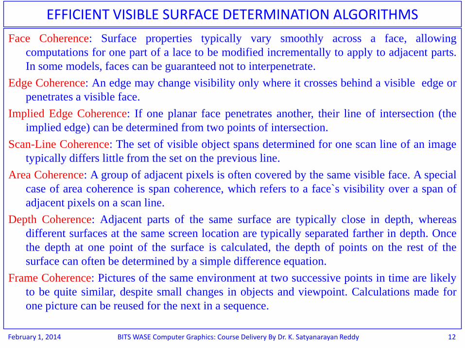
Face Coherence: Surface properties typically vary smoothly across a face, allowing

computations for one part of a lace to be modified incrementally to apply to adjacent parts.

In some models, faces can be guaranteed not to interpenetrate.

Edge Coherence: An edge may change visibility only where it crosses behind a visible edge or

penetrates a visible face.

Implied Edge Coherence: If one planar face penetrates another, their line of intersection (the

implied edge) can be determined from two points of intersection.

Scan-Line Coherence: The set of visible object spans determined for one scan line of an image

typically differs little from the set on the previous line.

Area Coherence: A group of adjacent pixels is often covered by the same visible face. A special

case of area coherence is span coherence, which refers to a face`s visibility over a span of

adjacent pixels on a scan line.

Depth Coherence: Adjacent parts of the same surface are typically close in depth, whereas

different surfaces at the same screen location are typically separated farther in depth. Once

the depth at one point of the surface is calculated, the depth of points on the rest of the

surface can often be determined by a simple difference equation.

Frame Coherence: Pictures of the same environment at two successive points in time are likely

to be quite similar, despite small changes in objects and viewpoint. Calculations made for

one picture can be reused for the next in a sequence.


EFFICIENT VISIBLE SURFACE DETERMINATION ALGORITHMS

The Perspective TransformationVisible Surface Determination clearly must be done in a 3D space prior to the

projection into 2D which destroys the depth information needed for depth

comparisons.

Given points Pl = (x1, yl, zl) and P2 = (x2, y2, z2), then for a perspective projection,

four divisions must be performed to determine whether

xl / zl = x2 / z2 and yl / zl = y2 / z2, in which case the points are on the same projector, as

shown in Fig. 15.10.

Moreover, if Pl is later compared against some point P3 = (x3, y3, z3), then two more

divisions are required.


Unnecessary divisions can be avoided by first transforming a 3D object into the 3D screen

coordinate system, so that the parallel projection of the transformed object is the same as the

perspective projection of the un-transformed object.

Then the test for one point obscuring another is the same as for parallel projections. This

perspective transformation distorts the objects and moves the center of projection to infinity

on the positive z axis, making the projectors parallel.

Figure 15.11 shows the effect of this transformation on the perspective view volume;


The Perspective Transformation cont’d….

Fig. 15. 12 shows how a cube is distorted by the transformation.



The division, which accomplishes the foreshortening, is done just once perpoint, rather than each time TWO points are compared. The matrix fromEq. (6.48)

transforms the normalized perspective view volume into the rectangularparallelepiped bounded by

Clipping can be done against the normalized truncated-pyramid view volumebefore the matrix M (defined above) is applied, but then the clipped resultsmust be multiplied by M.

An alternative is to incorporate M into the perspective normalizingtransformation Nper so that just a single matrix multiplication is needed, andthen to clip in homogeneous coordinates prior to the division.

If the results of this multiplication is (X, Y, Z, W), then, for W > 0, theclipping limits become



These limits are derived from Eq. (15,2)

by replacing x, y, and z by X/W, Y/W,

and Z/W respectively, to reflect the fact

that x, y and z in Eq. (15.2) result from

division by W.

After clipping, and dividing by W (xp, yp,

zp) is obtained.



Extents and Bounding VolumesScreen extents, to avoid unnecessary clipping, are also commonly used to avoid

unnecessary comparisons between objects or their projections.

Figure 15.13 shows two objects (3D polygons), their projections, and the upright

rectangular screen extents surrounding the projections.

The objects are assumed to have been transformed by the perspective transformation

matrix M (of Section 15.2.2).

Therefore, for polygons, orthographic projection onto the (x, y) plane is done trivially

by ignoring each vertex’s z coordinate.

In Fig. 15.13, the extents do not overlap, so the projections do not need to be tested for

overlap with one another.


If the extents overlap, one of two casts occurs, as shown in Fig. 15.14

either the projections also overlap, as in part (a), or they do not, as in

part (b).

In both cases, more comparisons must be performed to determine

whether the projections overlap in part (b), the comparisons will

establish that the two projections really do not intersect; in a sense,

the overlap of the extents was a false alarm.

Extent testing thus provides a service similar to that of trivial reject

testing in clipping.


Extents and Bounding Volumes cont’d….

There

Rectangular-extent testing is also known as bounding-box testing.

Extents can be used to surround the objects themselves rather than

their projections: in this case, the extents become solids and are also

known as bounding volumes.

Alternatively, extents can be used to bound a single dimension, in order

to determine, say, whether or not two objects overlap in z.

Figure 15.15 shows the use of extents in such a case; here, an extent is

the infinite volume bounded by the minimum and maximum z values

for each object.



There is no overlap in z ifZmax2 < Zmin1 OR Zmax1< Zmin2 ………….(15.4)

Comparing against minimum and maximumbounds in one or more dimensions is also knownas mimnax testing.

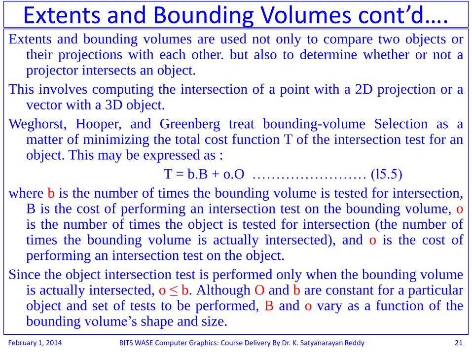
Extents and bounding volumes are used not only to compare two objects ortheir projections with each other. but also to determine whether or not aprojector intersects an object.

This involves computing the intersection of a point with a 2D projection or avector with a 3D object.

Weghorst, Hooper, and Greenberg treat bounding-volume Selection as amatter of minimizing the total cost function T of the intersection test for anobject. This may be expressed as :

T = b.B + o.O …………………… (l5.5)

where b is the number of times the bounding volume is tested for intersection,B is the cost of performing an intersection test on the bounding volume, ois the number of times the object is tested for intersection (the number oftimes the bounding volume is actually intersected), and o is the cost ofperforming an intersection test on the object.

Since the object intersection test is performed only when the bounding volumeis actually intersected, o ≤ b. Although O and b are constant for a particularobject and set of tests to be performed, B and o vary as a function of thebounding volume’s shape and size.



A “Tighter" bounding volume, which minimizes o, is typically associated with a

greater B.

A bounding volume’s effectiveness may also depend on an object’s orientation or the

kind of objects with which that object will be intersected.

Compare the two bounding volumes for the wagon wheel shown below in Fig. 15.16;

if the object is to be intersected with projectors perpendicular to the (x, y) plane,

then the tighter bounding volume is the sphere.



Back-Face Culling If an object is approximated by a solid polyhedron, then its polygonal faces completely enclose

its volume.

Assume that all the polygons have been defined such that their surface normals point out of

their polyhedron.

If none of the polyhedrons interior is exposed by the front clipping plane, then those polygons

whose surface normals point away from the observer lie on a part of the polyhedron whose

visibility is completely blocked by other closer polygons, as shown in Fig. l5.l7.

Such invisible back-facing polygons can be eliminated from further processing, a technique

known as back-face culling. By analogy, those polygons that are not back-facing are often

called front-facing.


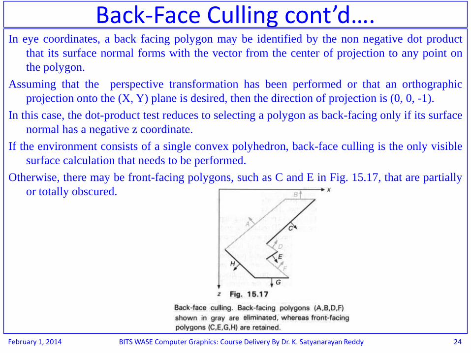
In eye coordinates, a back facing polygon may be identified by the non negative dot product

that its surface normal forms with the vector from the center of projection to any point on

the polygon.

Assuming that the perspective transformation has been performed or that an orthographic

projection onto the (X, Y) plane is desired, then the direction of projection is (0, 0, -1).

In this case, the dot-product test reduces to selecting a polygon as back-facing only if its surface

normal has a negative z coordinate.

If the environment consists of a single convex polyhedron, back-face culling is the only visible

surface calculation that needs to be performed.

Otherwise, there may be front-facing polygons, such as C and E in Fig. 15.17, that are partially

or totally obscured.


Back-Face Culling cont’d….

The Back Face Culling is an object-precision technique that requires time

linear in the number of polygons.

Sublinear performance can be Obtained by preprocessing the objects to be

displayed.

e.g.: Consider a cube centered about the origin of its own object coordinate

system, with its faces perpendicular to the coordinate system`s axes.

From any viewpoint outside the cube, at most three of its faces are

visible.

Furthermore, each Octant of the cubes coordinate system is associated

with a specific set of three potentially visible faces.

Therefore, the position of the viewpoint relative to the cubes coordinate

system can be used to select one of the eight sets of three potentially

visible faces.

For objects with a relatively small number of faces, a table may be made up

in advance to allow visible-surface determination without processing all

the object’s faces for each change of viewpoint.February 1, 2014 BITS WASE Computer Graphics: Course Delivery By Dr. K. Satyanarayan Reddy 25

Back-Face Culling cont’d….

Spatial PartitioningSpatial Partitioning (also known as Spatial Subdivision) allows one to

break down a large problem into a number of smaller ones.

The basic approach is to assign objects or their projections to spatially

coherent groups as a preprocessing step.

e.g.: The projection plane can be divided with a coarse, regular 2D

rectangular grid and determine in which grid spaces each object’s

projection lies.

Projections need to be compared for overlap with only those other

projections that fall within their grid boxes.

Spatial partitioning can be used to impose a regular 3D grid on the

objects in the environment. The process of determining which

objects intersect with a projector can then be sped up by first

determining which partitions the projector intersects, and then testing

only the objects lying within those partitions.


If the objects being depicted are unequally distributed

in space, it may be more efficient to use Adaptive

Partitioning, in which the size of each partition

varies.

One approach to adaptive partitioning is to subdivide

space recursively until some termination criterion is

fulfilled for each partition.

e.g.: Subdivision may stop when there are fewer than

some maximum number of objects in a partition.

The Quadtree, Octree, and BSP-Tree data structures

are particularly attractive for this purpose.


Spatial Partitioning cont’d….

HierarchyHierarchies can be useful for relating the structure and motion of different objects.

A nested hierarchical model, in which each child is considered part of its parent, can also be

used to restrict the number of object comparisons needed by a visible-surface algorithm.

An object on one level of the hierarchy can serve as an extent for its children if they are

entirely contained within it, as shown in Fig. 15.18.

In this case, if two objects in the hierarchy fail to intersect, the lower-level objects of one do

not need to be tested for intersection with those of the other.

Similarly, only if a projector is found to penetrate an object in the hierarchy then it must be

tested against the object‘s children.

This use of hierarchy is an important instance of object coherence.


ALGORITHMS FOR VISIBLE LINE DETERMINATION

Roberts's Algorithm : It requires that each edge be part of the face

of a convex polyhedron. First, back face culling is used to

remove all edges shared by a pair of a polyhedron’s back-facing

polygons.

Next, each remaining edge is compared with each polyhedron that

might obscure it.

Robert’s visibility test is performed with a parametric version of

the projector from the eye to a point on the edge being tested.

This method uses a linear-programming approach to solve for

those values of the line equation that cause the projector to pass

through a polyhedron, resulting in the invisibility of the

endpoint.

The projector passes through a polyhedron if it contains some

point that is inside all the polyhedron`s front faces.February 1, 2014 BITS WASE Computer Graphics: Course Delivery By Dr. K. Satyanarayan Reddy 29

Appel's Algorithm Appel defines the quantitative invisibility of a point on a line as the number of front-facing polygons that obscure that

point.

When a line passes behind at front-facing polygon, its quantitative invisibility is incremented by 1; when it passes out from

behind that polygon, its quantitative invisibility is decremented by l.

A line is visible only when its quantitative invisibility is 0. Line AB in Fig. 15. 19 is annotated with the quantitative

invisibility of each of its segments.

If interpenetrating polygons are not allowed. a line’s quantitative invisibility changes only when it passes behind what

Appel calls a contour line.

A contour line is either an edge shared by a front-facing and a back-facing polygon, or the unshared edge of a front-facing

polygon that is not part of a closed polyhedron.

An edge shared by two front-facing polygons causes no change in visibility and therefore is not a contour line.

In Fig. 15.19, edges AB. CD, DF, and KL are contour lines, whereas edges CE, EF, and JK are not.


The algorithm first computes the quantitative invisibility of a "seed" vertex ofan object by determining the number of front-facing polygons that hide it.

This can be done by a brute-force computation of all front-facing polygonswhose intersection with the projector to the seed vertex is closer than is theseed vertex itself.

The algorithm then takes advantage of edge coherence by propagating thisvalue along the edges emanating from the point, incrementing ordecrementing the value at each point at which an edge passes behind acontour line.

Only sections of edges whose quantitative invisibility is zero are drawn. Wheneach line’s other endpoint is reached, the quantitative invisibility associatedwith that endpoint becomes the initial quantitative invisibility of all linesemanating in turn from it.

One or more lines emanating from the vertex may be hidden by one or morefront-facing polygons sharing the vertex.

e.g.: In Fig. 15.19, edge JK has a quantitative invisibility of 0, while edge KLhas a quantitative invisibility of l because it is hidden by the object’s topface.

This change in quantitative invisibility at a vertex can be taken into account bytesting the edge against the front-facing polygons that share the vertex.


Appel's Algorithm cont’d….

Haloed Lines Appel, Rohlf, and Stein describe an algorithm for rendering haloed lines, as shown in Fig. 15.20.

Each line is surrounded on both sides by a halo that obscure those parts of lines passing behind it. This

algorithm, unlike those discussed previously, does not require each line to be part of an opaque

polygonal face.

Lines that pass behind others are obscured only around their intersection on the view plane.

The algorithm intersects each line with those passing in front of it, keeps track of those sections that are

obscured by halos, and draws the visible sections of each line after the intersections have been

calculated.

lf the halos are wider than the spacing between lines, then an effect similar to conventional hidden-line

elimination is achieved, except that a line’s halo extends outside a polygon of which it may be an edge.


THE z-BUFFER ALGORITHM The z-buffer or depth-buffer image-precision algorithm, developed by

Catmull, is one of the simplest visible-surface algorithms to implement in

either software or hardware.

It requires that we have available not only a Frame Buffer F in which color

values are stored, but also a z-buffer Z, with the same number of entries, in

which a z-value is stored for each pixel.

The z-buffer is initialized to zero, representing the z-value at the back

clipping plane, and the frame buffer is initialized to the background color.

The largest value that can be stored in the z-buffer represents the z of the front

clipping plane.

Polygons are scan-converted into the frame buffer in arbitrary order. During

the scan-conversion process, if the polygon point being scan-converted at

(x, y) is no farther from the viewer than is the point whose color and depth

are currently in the buffers, then the new point’s color and depth replace

the old values.

The pseudocode for the z-buffer algorithm is shown in Fig. l5.2l.



THE z-BUFFER ALGORITHM cont’d….

The WritePixel andReadPixel proceduresare supplemented hereby WriteZ and ReadZprocedures that writeand read the z-buffer.

No presorting is necessary and no object-object comparisons are required.

The entire process is no more than a search over each set of pairs {Zi(x ,y), Fi(x, y)} for fixed x and y, to find the

largest Zi.

The z-buffer and the frame buffer record the information associated with the largest z encountered so far for each

(x, y). Thus, polygons appear on the screen in the order in which they are processed. Each polygon may be

scan-converted one scan line at a time into the buffers. Figure 15.22 shows the addition of two polygons to an

image. Each pixel‘s shade is shown by its color; its z is shown as a number.



The calculation of z for each point on a scan line can be simplified

by exploiting the fact that a polygon is planar.

Normally to calculate z, the plane equation A.x + By + Cz + D =

U would have to be solved for the variable z

Now, if at (x, y) Eq. (15.6) evaluates to z1, then at (x + Δx, y) the

value of z is

Only one subtraction is needed to calculate z(x + 1, y) given z(x,

y), since the quotient A/C is constant and Δx = 1.

A similar incremental calculation can be performed to determine

the first value of z on the next scan line, decrementing by B/C

for each Δ y.



Alternatively, if the surface has not been determined or if the polygon is

not planar, z(x, y) can be determined by interpolating the z

coordinates of the polygon‘s vertices along pairs of edges, and then

across each scan line, as shown in Fig. 15.23. Incremental

calculations can be used here.

Note: the color at a pixel does not need to be computed if the

conditional determining the pixe1’s visibility is not satisfied.

Therefore, if the shading computation is time consuming, additional

efficiency can be gained by performing a rough front-to-back depth

sort of the objects to display the closest objects first.

The z-buffer algorithm does not require that objects be polygons.

Indeed, one of its most powerful attractions is that it can be used to

render any object if a shade and a z-value can be determined for each

point in its projection; no explicit intersection algorithms need to be

written.



The z-buffer algorithm performs radix sorts in x and y, requiring nocomparisons, and its z sort takes only one comparison per pixel for eachpolygon containing that pixel.

The time taken by the visible-surface calculations tends to be independent ofthe number of polygons in the objects because, on the average, the numberof pixels covered by each polygon decreases as the number of polygons inthe view volume increases.

Therefore, the average size of each set of pairs being searched tends to remainfixed.

Although the z-buffer algorithm requires a large amount of space for the z-buffer, it is easy to implement.

If memory is at a premium, the image can be scan-converted in strips, so thatonly enough z-buffer for the strip being processed is required, at theexpense of performing multiple passes through the objects.

Because of the z-buffer’s simplicity and the lack of additional data structures,decreasing memory costs have inspired a number of hardware andfirmware implementations of the z-buffer.

Because the z-buffer algorithm operates in Image Precision, however, it issubject to aliasing.



Advantages of z-Buffer: Even after the image has been

rendered, the z-buffer can still be used to advantage.

Since it is the only data structure used by the visible-surface

algorithm proper, it can be saved along with the image and

used later to merge in other objects whose z can be

computed.

The algorithm can also be coded so as to leave the z-buffer

contents unmodified when rendering selected objects.

If the z-buffer is masked off this way, then a single object can

be written into a separate set of overlay planes with hidden

surfaces properly removed (if the object is a single-valued

function of x and y) and then erased without affecting the

contents of the z-buffer.February 1, 2014 BITS WASE Computer Graphics: Course Delivery By Dr. K. Satyanarayan Reddy 39


Thus, a simple object, such as a ruled grid, can

be moved about the image in x, y, and z. to

serve as a "3D cursor" that obscures and is

obscured by the objects in the environment.

Cutaway views can be created by making the z-

buffer and frame-buffer writes contingent on

whether the z value is behind a cutting plane.

If the objects being displayed have a single z

value for each (x, y), then the z-buffer contents

can also be used to compute area and volume.



LIST-PRIORITY ALGORITHMSList-priority algorithms determine a visibility ordering for objects ensuring that a correct

picture results if the objects are rendered in that order. For example, if no object

overlaps another in 2, then the objects need only to sorted by increasing z, and to

render them in that order.

Farther objects are obscured by closer ones as pixels from the closer polygons overwrite

those of the more distant ones.

If objects overlap in z, we may still be able to determine a correct order, as in Fig. l5.24(a).

If objects cyclically overlap each other, as Fig. 15.24(b) and (c). or penetrate each

other, then there is no correct order. In these cases, it will be necessary to split one or

more objects to make a linear order possible.


List—priority algorithms are hybrids that combine both

object—precision and image- precision operations.

Depth comparisons and object splitting are done with object

precision. Only scan conversion, which relies on the ability

of the graphics device to overwrite the pixels of previously

drawn objects. is done with image precision.

Because the list of sorted objects is created with object

precision, however, it can be redisplayed correctly at any

resolution.

The sorting need not be on z, some objects may be split that

neither cyclically overlap nor penetrate others, and the

splitting may even be done independent of the viewer's

position.February 1, 2014 BITS WASE Computer Graphics: Course Delivery By Dr. K. Satyanarayan Reddy 42

LIST-PRIORITY ALGORITHMS cont’d….

The Depth-Sort (Painter’s) AlgorithmThe basic idea of the depth-sort algorithm, developed by

Newell, Newell, and Sancha, is to paint the polygons

into the frame buffer in order of decreasing distance

from the viewpoint.

Three conceptual steps are performed;

l. Sort all polygons according to the smallest (farthest) z

coordinate of each

2. Resolve any ambiguities this may cause when the

polygon’s z extents overlap, splitting polygons if

necessary

3. Scan convert each polygon in ascending order of

smallest z coordinate (i.e., back to front).February 1, 2014 BITS WASE Computer Graphics: Course Delivery By Dr. K. Satyanarayan Reddy 43

This simplified version of the depth-sort algorithm is often known

as the Painters algorithm, in reference to how a painter might

paint closer objects over more distant ones.

Environments whose objects each exist in a plane of constant z,

such as those of VLSI layout, cartography, and window

management, are said to be 2Q-D and can be correctly handled

with the painters algorithm.

The painter’s algorithm may be applied to a scene in which each

polygon is not embedded in a plane of constant z by sorting the

polygons by their minimum z coordinate or by the z coordinate

of their centroid, ignoring step 2.

Although scenes can be constructed for which this approach

works, it does not in general produce a correct ordering.


The Depth-Sort (Painter’s) Algorithm cont’d….

Figure 15.24 above shows some of the types of ambiguities

that must be resolved as part of step 2. How is this done?

Let the polygon currently at the far end of the sorted list of

polygons be called P. Before this polygon is scan-

converted into the frame buffer, it must be tested against

each polygon Q whose z extent overlaps the z extent of

P, to prove that P cannot obscure Q and that P can

therefore be written before Q.

Up to five tests are performed, in order of increasing

complexity. As soon as one succeeds, P has been shown

not to obscure Q and the next polygon Q overlapping P

in z is tested.



If all such polygons pass, then P is scan-converted and the next polygon on the list becomes the new P. The five

tests are

l. Do the polygons` x extents not overlap'?

2. Do the polygons’ y extents not overlap?

3. Is P entirely on the opposite side of Q’s plane from the viewpoint? (This is not the case in Fig. l5.24(a). but

is true for Fig. 15.25.)

4. Is Q entirety on the same side of P‘s plane as the viewpoint? (This is not the case in Fig. l5.24(a), but is

true for Fig. l5.26.)

5. Do the projections of the polygons onto the (x. y) plane not overlap'? (This can be determined by

comparing the edges of one polygon to the edges of the other.)

If all five tests fail. assuming for the moment that P actually obscures Q, and therefore test whether Q can be scan-

converted before P. Tests 1, 2, and 5 do not need to be repeated, but new versions of tests 3 and 4 are used,

with the polygons reversed:

3'. Is Q entirely on the opposite side of P’s plane from the viewpoint'?

4'.Is P entirely on the same side of Q'; plane as the viewpoint?



Binary Space-Partitioning TreesThe Binary Space Partitioning (BSP) tree algorithm, developed by Fuchs, Kedem, and Naylor,

is an extremely efficient method for calculating the visibility relationships among a static

group of 3D polygons as seen from an arbitrary viewpoint.

It trades off an initial time and space intensive preprocessing step against a linear display

algorithm that is executed whenever a new viewing specification is desired.

Thus, the algorithm is well suited for applications in which the viewpoint changes, but the

objects do not.

The BSP tree algorithm is based on the work of Schumacker, who noted that environments can

be viewed as being composed of clusters (collections of faces), as shown in Fig. l5.28(a).


If a plane can be found that wholly separates one set of clusters fromanother. then clusters that are on the same side of the plane as theeyepoint can obscure, but cannot be obscured by, clusters on theother side.

Each of these sets of clusters can be recursively subdivided if suitableseparating planes can be found. As shown in Fig. l5.28(b), thispartitioning of the environment can be represented by a binary treerooted at the first partitioning plane chosen.

The tree's internal nodes are the partitioning planes; its leaves areregions in space. Each region is associated with a unique order inwhich clusters can obscure one another if the viewpoint is located inthat region.

Determining the region in which the eyepoint lies involves descendingthe tree from the root and choosing the left or right child of aninternal node by comparing the viewpoint with the plane at thatnode.


Binary Space-Partitioning Trees cont’d….

Schumacker selects the faces in a cluster so that a priority ordering can be assigned to each face

independent of the viewpoint, as shown in Fig. 15.29.

After back-face culling has been performed relative to the viewpoint, a face with a lower

priority number obscures a face with a higher number wherever the faces' projections

intersect.

For any pixel, the correct face to display is the highest-priority (lowest-numbered) face in the

highest-priority cluster whose projection covers the pixel. Schumacker used special

hardware to determine the front most Face at each pixel.

It is based on the observation that a polygon will be scan-converted correctly, if all polygons on

the other side of it from the viewer are scan-converted first, then it, and then all polygons on

the same side of it as the viewer.



The algorithm makes it easy to determine a correct order for scan conversion

by building a binary tree of polygons, the BSP tree.

The BSP trees root is a polygon selected from those to be displayed; the

algorithm works correctly no matter which is picked.

The root polygon is used to partition the environment into two half-spaces.

One half—space contains all remaining polygons in front of the root polygon,

relative to its surface normal; the other contains all polygons behind the

root polygon.

Any polygon lying on both sides of the root polygon’s plane is split by the

plane and its front and back pieces are assigned to the appropriate half

space.

One polygon each from the root polygon ’s from and back half space become

its front and back children, and each child is recursively used to divide the

remaining polygons in its half space in the same fashion.

The algorithm terminates when each node contains only a single polygon.

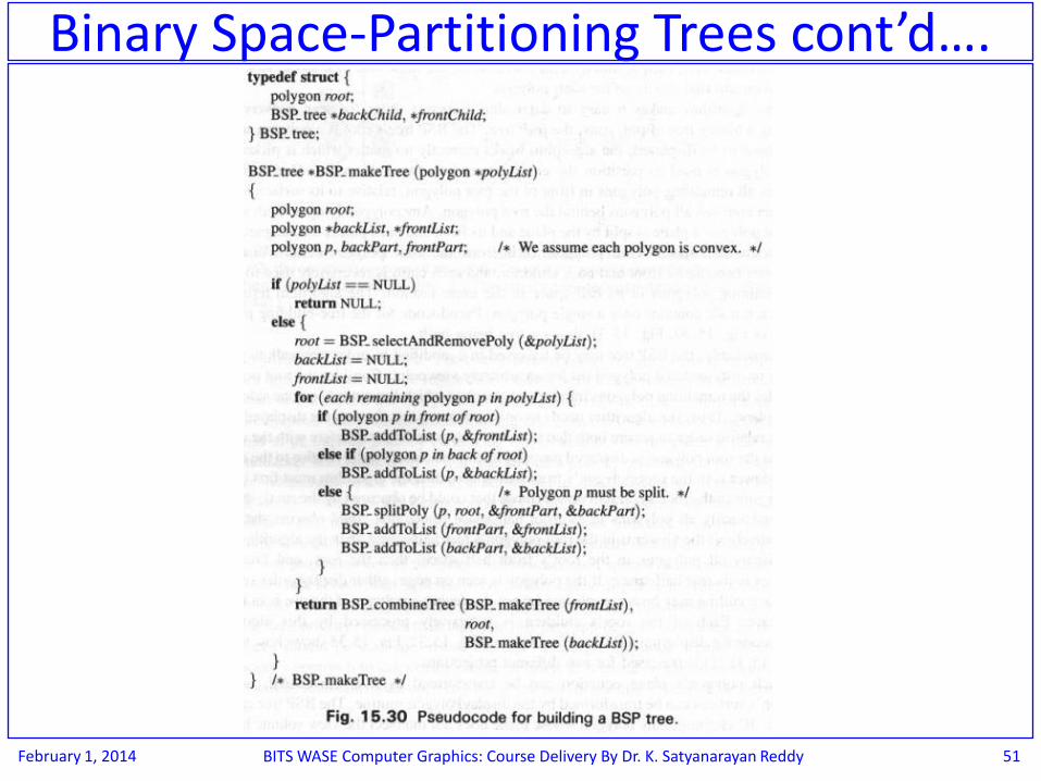
Pseudocode for the tree-building phase is shown in Fig. 15.30;



Fig. 15.31 shows a tree being built.



THANK YOU


bits wase computergraphics session 13 14

Documents