black-box modeling and attitude control of a quadcopterabstract in this thesis, black-box models...

Master of Science Thesis in Electrical Engineering

Department of Electrical Engineering, Linköping University, 2016

Black-Box Modeling and

Attitude Control of a

Quadcopter

Ingrid Kugelberg

Master of Science Thesis in Electrical EngineeringBlack-Box Modeling and Attitude Control of a Quadcopter

Ingrid KugelbergLiTH-ISY-EX–16/4927–SE

Supervisor: Jonas Linderisy, Linköping University

Henrik JonsonSaab Dynamics AB

Examiner: Martin Enqvistisy, Linköping University

Division of Automatic Control

Department of Electrical Engineering

Linköping University

SE-581 83 Linköping, Sweden

Copyright © 2016 Ingrid Kugelberg

To my parents.

AbstractIn this thesis, black-box models describing the quadcopter system dynamics forattitude control have been estimated using closed-loop data. A quadcopter is anaturally unstable multiple input multiple output (MIMO) system and is there-fore an interesting platform to test and evaluate ideas in system identificationand control theory on. The estimated attitude models have been shown to ex-plain the output signals well enough during simulations to properly tune a PIDcontroller for outdoor flight purposes.

With data collected in closed loop during outdoor flights, knowledge aboutthe controller and IMU measurements, three decoupled models have been esti-mated for the angles and angular rates in roll, pitch and yaw. The models for rolland pitch have been forced to have the same model structure and orders sincethis reflects the geometry of the quadcopter. The models have been validated bysimulating the closed-loop system where they could explain the output signalswell.

The estimated models have then been used to design attitude controllers tostabilize the quadcopter around the hovering state. Three PID controllers havebeen implemented on the quadcopter and evaluated in simulation before beingtested during both indoor and outdoor flights. The controllers have been shownto stabilize the quadcopter with good reference tracking. However, the perfor-mance of the pitch controller could be improved further as there have been smalloscillations present that may indicate a stronger correlation between the roll andpitch channels than assumed.

v

AcknowledgmentsFirst of all, I would like to thank my amazing family, for always being there forme, supporting my decisions and for believing in me.

I would also like to thank my examiner Martin Enqvist and my supervisorJonas Linder from Linköping University for engaging in stimulating discussions,for their support and inspiration.

Finally, I would like to thank Torbjörn Crona, Henrik Jonson, Carl Nordheimand Anders Peterson for giving me the opportunity to write my thesis at SaabDynamics AB, and for all the support and help.

This thesis is dedicated to my parents.

Linköping, February 2016Ingrid Kugelberg

vii

Contents

Notation xi

1 Introduction 11.1 Background . . . . . . . . . . . . . . . . . . . . . . . . . . . . . . . 11.2 Problem Formulation . . . . . . . . . . . . . . . . . . . . . . . . . . 11.3 Goals . . . . . . . . . . . . . . . . . . . . . . . . . . . . . . . . . . . 21.4 Limitations . . . . . . . . . . . . . . . . . . . . . . . . . . . . . . . . 21.5 Thesis Outline . . . . . . . . . . . . . . . . . . . . . . . . . . . . . . 3

2 The Quadcopter Platform 52.1 Hardware . . . . . . . . . . . . . . . . . . . . . . . . . . . . . . . . . 52.2 Software . . . . . . . . . . . . . . . . . . . . . . . . . . . . . . . . . 6

2.2.1 Navigation . . . . . . . . . . . . . . . . . . . . . . . . . . . . 72.2.2 Guidance and Control . . . . . . . . . . . . . . . . . . . . . 7

2.3 Quadcopter Modeling . . . . . . . . . . . . . . . . . . . . . . . . . . 10

3 Model Estimation 153.1 System Identification . . . . . . . . . . . . . . . . . . . . . . . . . . 153.2 Closed-loop System Identification . . . . . . . . . . . . . . . . . . . 173.3 Data Collection . . . . . . . . . . . . . . . . . . . . . . . . . . . . . 183.4 Estimated Attitude Models . . . . . . . . . . . . . . . . . . . . . . . 18

3.4.1 Roll and Pitch . . . . . . . . . . . . . . . . . . . . . . . . . . 193.4.2 Yaw . . . . . . . . . . . . . . . . . . . . . . . . . . . . . . . . 29

4 Control Design 334.1 Feedback Control . . . . . . . . . . . . . . . . . . . . . . . . . . . . 334.2 Implementation Aspects . . . . . . . . . . . . . . . . . . . . . . . . 354.3 Attitude Controller . . . . . . . . . . . . . . . . . . . . . . . . . . . 36

4.3.1 Roll Controller . . . . . . . . . . . . . . . . . . . . . . . . . 374.3.2 Pitch Controller . . . . . . . . . . . . . . . . . . . . . . . . . 404.3.3 Yaw Controller . . . . . . . . . . . . . . . . . . . . . . . . . . 43

4.4 Simulation . . . . . . . . . . . . . . . . . . . . . . . . . . . . . . . . 464.5 Outdoor and Indoor Flights . . . . . . . . . . . . . . . . . . . . . . 48

ix

x Contents

5 Conclusions and Future Work 535.1 Conclusions . . . . . . . . . . . . . . . . . . . . . . . . . . . . . . . 535.2 Future Work . . . . . . . . . . . . . . . . . . . . . . . . . . . . . . . 54

Bibliography 55

Notation

Abbreviations

Abbreviation Meaning

gc Guidance and control software unitnav Navigation software unitpid Proportional, integral, derivative (controller)

Rigid-body Generalized Positions

Variable Description

x Longitudinal position relative the inertial framey Lateral position relative the inertial framez Vertical position relative the inertial frame� Roll angle relative the inertial frame✓ Pitch angle relative the inertial frame Yaw angle relative the inertial frame

Rigid-body Generalized Velocities

Variable Description

u Linear velocity in x-axis of the body-fixed framev Linear velocity in y-axis of the body-fixed framew Linear velocity in z-axis of the body-fixed framep Roll rate, angular velocity around the x-axis of the

body-fixed frameq Pitch rate, angular velocity around the y-axis of the

body-fixed framer Yaw rate, angular velocity around the z-axis of the

body-fixed frame

xi

1Introduction

This is the report of a performed at Saab Dynamics in Linköping, Sweden. Thischapter aims to give the reader an overview and introduction to this investigatedproblem. The background, goals and limitations of the thesis are discussed. Fur-thermore, the methods used to carry out the master’s thesis and related work arepresented. Finally, a brief overview of the disposition of the report is given.

1.1 Background

The use of unmanned areal vehicles (UAVs), or drones, has many interestingapplications. Beyond the uses within military applications, UAVs can performsearch and rescue operations in hazardous environments, surveillance and in-spections of hard to reach places (Waharte and Trigoni, 2010; Nikolic et al., 2013).UAVs can even be used for acrobatic aerial footage in the filmmaking industry orin the future for home delivery of purchased goods (Zhang et al., 2014).

One type of an UAV is a multicopter that is equipped with a control system.This is an agile, flying platform that can be modified in size and capabilities forwhatever application the designer has in mind. A multicopter is the designationof a rotorcraft with more than two rotors and a quadcopter is the designation forthe special case of four rotors.

1.2 Problem Formulation

There has been a lot of research conducted to study quadcopters (Yungao et al.,2011; Gupte et al., 2012; Nagarjuna and Suresh, 2015; Cutler, 2012; Mustapaet al., 2014). Data-based modeling or system identification is an interesting butdi�cult task and there are many aspects to consider for how it should be done.

1

2 1 Introduction

A quadcopter is a naturally unstable multiple input multiple output (MIMO)system. Moreover, since the data collection for the system identification will bemade outdoors during flight, and not in a testbench, this unstable system willrequire feedback. The platform will be equipped with initial stabilizing PID con-trollers to make the quadcopter airworthy.

During data collection it is important to excite the system to obtain data thatis informative enough in order to successfully perform system identification (Bel-tramini et al., 2011). It is assumed that the pilot conducting the experiments isnot an experienced quadcopter acrobatics pilot which means that the complexityand approaches of the test flights cannot be designed as arbitrarily as desired.

A common approach when performing system identification is to use a grey-box model, which means to use a physical model of the system but to let someparameters be estimated through experiments (Li, 2014). The second alternativeis to use a black-box model which does not take any physical constraints intoconsideration and only relies on data from test flights to create a predictive math-ematical model of the system (Ljung, 2001; Panizza et al., 2015).

After a model of the system has been estimated, a controller should be de-signed and implemented to replace the PID controllers that were implementedon the platform initially. In order to handle wind and other disturbances, thecontroller design has to be robust towards these disturbances and towards modelerrors.

1.3 Goals

The main objectives for this master’s thesis was to perform system identificationof a quadcopter and to design and implement a controller. The final estimatedmodel of the system should be a foundation for future work on the platform. Thecontroller should be designed to control the di↵erent dynamics of the quadcopterwhile in the hovering state and close to hovering.

1.4 Limitations

All hardware components and configurations was provided for by Saab Dynam-ics. There was no time spent working on the hardware in this thesis project.

The data collection was performed outdoors where high-speed flights couldbe conducted and the necessary precautions could be taken into consideration.Since the wind caused minor problems the data collection was performed whenthere was as little wind as possible. There was a human pilot conducting theexperiments and this imposed a limitation since an arbitrary input could not beused.

1.5 Thesis Outline 3

1.5 Thesis OutlineThis thesis is divided into five chapters and is organized as follows. Chapter 2presents the setup of the quadcopter platform, describing the hardware and soft-ware solutions, and a physical model of the quadcopter is also derived there.The next chapter, Chapter 3, treats some system identification theory and theapproaches taken and the resulting attitude models.

In Chapter 4, control theory and implementation aspects are presented, fol-lowed by the controller design and a discussion regarding the results from boththe simulations and the outdoor flights. Finally, in Chapter 5 some final conclu-sions are presented and future work on the platform is discussed.

2The Quadcopter Platform

A quadcopter is a naturally unstable platform. By changing the relative speed ofthe rotors, motion in roll, pitch and yaw can be achieved, creating lateral and lon-gitudinal thrust. Quadcopters are relatively cheap and come in all sizes makingthem a suitable platform for research.

This chapter treats the quadcopter platform that was used for this thesis. Itis explained which hardware it is built of and which software solutions that wereused. As previously mentioned in Section 1.4, the platform was provided by SaabDynamics AB. Therefore, this chapter only aims at giving the reader an overviewof the system. Finally, a physical model of the quadcopter will be presented.

2.1 Hardware

The complete setup weighs about 680 grams. The specific quadcopter used forthis master’s thesis can be seen in Figure 2.1. The frame is an QAV250 Mini FPV,seen in Figure 2.2, and it is assumed to be rigid. It is designed for hobby users,with plenty of space along the center line to allow for additional equipment to beattached, for example, a camera, and o↵ers plenty of flexibility for the assembler.As can be seen in Figure 2.1, the quadcopter has four propellers and one motorto control each of them. The motors used are the FX2206-13 2000kv, which arebrushless motors. The propellers used on the platform are the GEMFAN 5X3.Each motor is controlled by an electronic speed controller (ESC). The ESC re-ceives a command from the quadcopter control unit and delivers the requiredpower to its motor. The ESCs used on the platform are the Luminier Mini 20A.They are small in size but they can deliver high power and are recommendedfor this frame. To supply the quadcopter with power, the battery Lumenier 1300

mAh 35c Lipo Battery (XT60) is used. Its small size allows it to fit on the quad-copter frame and, for this specific setup, the battery o↵ers about 5 minutes of

5

6 2 The Quadcopter Platform

Figure 2.1: A photo of the quadcopter platform used. The quadcopter has

four propellers. Each one has a motor and an electric speed controller (ESC).

The ESC and all other electronics are attached along the lateral center line of

the quadcopter. There is also additional free space left on the frame, allow-

ing for an action camera to be attached in the future.

flight time. The transmitter used here is the FrSky Taranis X9D Plus. The unitfeatures a multicolored display and vibration alerts. In line with the industrystandard, it has the throttle/rudder stick to the left and the elevator/aileron stickto the right. The receiver used is a FrSky X8R, which is very small and light andtherefore suitable in this application. Finally, the flight controller consists of anArduino Micro, a Raspberry Pi, a pulse width modulation (PWM) module and aninertial measurement unit (IMU).

Figure 2.2: A photo of the quadcopter frame used, the QAV250 Mini FPV.The frame is made by Luminier. It is designed to support powerful motors

and has an integrated power distribution board for the ESCs and flight elec-

tronics.

2.2 Software 7

2.2 Software

In this section, the software solutions used on the platformwill be explained. Theflight controller is the main software component and the setup is illustrated inFigure 2.3.

The Raspberry Pi has the Guidance and Control unit (GC), the Navigationunit (NAV) and three daemons; the Receiver daemon, the PWM daemon andthe Logger daemon. The Receiver daemon stores the latest control commandreceived from the transmitter and, upon request from the GC, sends it to the GCalong with a flag. The flag indicates whether or not the control command is new,or the same as the previous command. This allows for good debugging propertiesof the flight controller.

The communication from the IMU to the Raspberry Pi and the communica-tion from the receiver to the Arduino and to the Raspberry Pi is done via Univer-sal Asynchronous Receiver/Transmitter (UART). All communication on the Rasp-berry Pi is via the User Data Protocol (UDP) and therefore is the PWM daemonnecessary in order to change protocol from UDP to Inter-Integrated Circuit (I2C),which the PWMmodule needs as input. The communication from the PWMmod-ule to the ESCs is done with analog PWM signals. The Logger daemon receivesand stores data from the GC.

Figure 2.3: An illustration of how the flight controller is set up. The dashed

line shows the flight controller setup and the dark grey box shows the soft-

ware components on the Raspberry Pi. The components communicating

with the flight controller are outside the dashed line.


Table 2.1: Stated accuracy of the navigation solution.

Navigation Solution AccuracyRoll Angle 0.1 degPitch Angle 0.1 degYaw Angle 1 degAngular Velocity 5.7 deg/s

2.2.1 NavigationThe Navigation unit (NAV) receives inputs from the IMU and sends out naviga-tion information to the GC. The inputs are processed on the Raspberry Pi and thesoftware is based on a discrete Extended Kalman Filter (EKF) for state estimation.The precision of the NAV can be seen in Table 2.1. The NAV is provided for bySaab Dynamics.

2.2.2 Guidance and ControlThe Guidance and Control unit (GC) is the main unit of the flight controller andone of the most important parts of the quadcopter. The GC receives navigation in-formation from the NAV and a steering input from the receiver. The GC uses thisinformation to compute a controller output for each of the four motors accordingto some control algorithm. Initially, the GC will use stabilizing PID controllers tomake the quadcopter airworthy but these will later be replaced with controllersdesigned using the estimated models.

One iteration of the flight controller loop will start when the GC receives amessage from the NAV. The process is illustrated in Figure 2.4. The goal is tominimize the controller latency as much possibly. Therefore, the GC will thencompute a controller output, according to the information stored in the Receiverdaemon, and send the controller output to the PWM daemon. These two stepsare the critical and determines the latency of the controller. Once these stepsare finished, data will be sent to the Logger daemon. The iteration will end withthe GC reading from the Receiver daemon, instead of doing this prior to theother steps. Finally, the GC stays idle for some time. However, this results in asmall delay of the pilot’s commands of about 10 ms but it was considered to beunnoticeable for the pilot.

2.3 Quadcopter Modeling 9

Figure 2.4: An illustration of the flow of the GC. The process begins when a

new NAV message is received. The time delay of the controller is dependent

on the first two steps of the sprint, when the controller computes and sends

the control output. The data is then logged, a new steering input is fetched

from the receiver and finally, the GC stays idle.

2.3 Quadcopter Modeling

In this section, a model of a quadcopter is presented. The model

⌘ = J(⌘)⌫ (2.1)

MRB⌫ + CRB(⌫)⌫ = ⌧ (2.2)

from Thornton and Marion (2004), presents a physical model for a rigid-body,where the vector

⌘ =hx y z � ✓

iT(2.3)

is the position and orientation of the quadcopter in the inertial frame and

⌫ =hu v w p q r

iT(2.4)

is the linear velocities and angular velocities of the quadcopter in the body-fixedframe, and

J(⌘) ="R(⌘) 03⇥303⇥3 T (⌘)

#(2.5)

is a transformation matrix of the orientation and position of the body frame withrespect to the inertial frame. Finally,MRB is the rigid-body inertia matrix, CRB(⌫)represents the centripetal and Coriolis terms and ⌧ is the generalized forces andtorques, all of which are expressed in the body-fixed frame.

The matrix in (2.5) is a transformation matrix with the rotation matrix

R(⌘) =

266666664

c c✓ �s c� + c s✓s� s s� + c c�s✓s c✓ c c� + s s✓s� �c s� + s c�s✓�s✓ c✓s� c✓c�

377777775

(2.6)


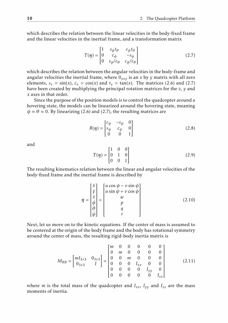
which describes the relation between the linear velocities in the body-fixed frameand the linear velocities in the inertial frame, and a transformation matrix

T (⌘) =

266666664

1 s� t✓ c� t✓0 c� �s�0 s�/c✓ c�/c✓

377777775

(2.7)

which describes the relation between the angular velocities in the body-frame andangular velocities the inertial frame, where 0x⇥y is an x by y matrix with all zeroelements, sx = sin(x), cx = cos(x) and tx = tan(x). The matrices (2.6) and (2.7)have been created by multiplying the principal rotation matrices for the z, y andx axes in that order.

Since the purpose of the positionmodels is to control the quadcopter around ahovering state, the models can be linearized around the hovering state, meaning� ⇡ ✓ ⇡ 0. By linearizing (2.6) and (2.7), the resulting matrices are

R(⌘) =

26666664

c �s 0s c 00 0 1

37777775 (2.8)

and

T (⌘) =

26666664

1 0 00 1 00 0 1

37777775 (2.9)

The resulting kinematics relation between the linear and angular velocities of thebody-fixed frame and the inertial frame is described by

⌘ =

266666666666666666664

xyz�✓

377777777777777777775

=

266666666666666666664

u cos � v sin u sin + v cos

wpqr

377777777777777777775

(2.10)

Next, let us move on to the kinetic equations. If the center of mass is assumed tobe centered at the origin of the body frame and the body has rotational symmetryaround the center of mass, the resulting rigid-body inertia matrix is

MRB ="mI3⇥3 03⇥303⇥3 I

#=

266666666666666666664

m 0 0 0 0 00 m 0 0 0 00 0 m 0 0 00 0 0 Ixx 0 00 0 0 0 Iyy 00 0 0 0 0 Izz

377777777777777777775

(2.11)

where m is the total mass of the quadcopter and Ixx, Iyy and Izz are the massmoments of inertia.


The centripetal and Coriolis terms are represented by the matrix

CRB(⌫)⌫ =

266666666666666666664

0 0 0 0 mw �mv0 0 0 �mw 0 mu0 0 0 mv �mu 00 0 0 0 Izz r �Iyyq0 0 0 �Izz r 0 Ixxp0 0 0 Iyyq �Ixxp 0

377777777777777777775

266666666666666666664

uvwpqr

377777777777777777775

(2.12)

In the hovering case, it can be assumed that all the linear velocities and all theangular velocities, except for r, are equal to zero. By linearizing (2.12) aroundu ⇡ v ⇡ w ⇡ p ⇡ q ⇡ 0, the resulting matrix is

CRB(⌫) =

266666666666666666664

0 �mr 0 0 0 0mr 0 0 0 0 00 0 0 0 0 00 0 0 0 (Izz � Iyy)r 00 0 0 (Ixx � Izz)r 0 00 0 0 0 0 0

377777777777777777775

(2.13)

which replaces (2.12) in (2.2).The generalized forces ⌧ can be divided into three components

⌧ = ⌧gravitational + ⌧damping + ⌧actuators = G(⌘) + D(⌫) + ⌧c(u) (2.14)

where G(⌘) is the gravitational component, D(⌫) is the damping component,⌧c(u) is the forces generated by the actuators and u is the input vector to themotors. The gravitational component is acting in the inertial z-direction. Bytranslating the force to the body frame, the resulting force is described by

G(⌘) =

266666666666666666664

�mg sin ✓mg cos ✓ sin�mg cos ✓ cos�

000

377777777777777777775

(2.15)

Since the hovering case is studied here, the angles � and ✓ are small and thesmall angle approximation can be used, where sin x ⇡ x and cos x ⇡ 1. This gives

G(⌘) =

266666666666666666664

�mg✓mg�mg000

377777777777777777775

(2.16)


The damping component is the linear matrix

D(⌫) = D0⌫ =

266666666666666666664

D0,uuD0,vvD0,wwD0,ppD0,qqD0,r r

377777777777777777775

(2.17)

where D0 are the linear damping coe�cients. The forces and torques generatedby the actuators are assumed to be linear in the input, hence

⌧c(u) = Ku =

266666666666666666664

00

KthrottleuthrottleKrolluroll

KpitchupitchKyawuyaw

377777777777777777775

(2.18)

where Kthrottle is the coe�cient of the force a↵ecting the velocity w is the z-direction and Kroll, Kpitch and Kyaw are the coe�cients of the torques about thebody-fixed coordinate axes. The resulting kinetic equations are

266666666666666666664

uvwpqr

377777777777777777775

=

266666666666666666664

(�mrv � mg✓)/m(mru + mg�)/m

(mg + Kthrottleuthrottle)/m((Izz � Iyy)qr + D0,pp + Krolluroll)/Ixx

((Ixx � Izz)pr + D0,qq + Kpitchupitch)/Iyy(D0,r r + Kyawuyaw)/Izz

377777777777777777775

(2.19)

The complete system dynamics of the quadcopter is given by (2.19) and (2.10).The four motors on the quadcopter are set up as in Figure 2.5. The controller

outputs, i.e. uthrottle, uroll, upitch and uyaw, are linear combinations of the fourmotor signals according to

266666666664

uthrottleurollupitchuyaw

377777777775=

14

266666666664

1 1 1 1�1 �1 1 11 �1 �1 1�1 1 �1 1

377777777775

266666666664

M1M2M3M4

377777777775

(2.20)

where M1, M2, M3 and M4 are the motor signals. This gives266666666664

M1M2M3M4

377777777775=

266666666664

1 �1 1 �11 �1 �1 11 1 �1 �11 1 1 1

377777777775

266666666664

uthrottleurollupitchuyaw

377777777775

(2.21)

which is how the controller outputs are mapped to the motors. The motor signalsare in a range of 0 to 1, which corresponds to the minimum and maximum signalpower that the ESCs can receive.


Figure 2.5: An illustration of the rotational directions of the four motors

on the quadcopter seen from above. Motors 1 and 3 are rotating clockwise

and motors 2 and 4 are rotating counterclockwise. The x-axis is pointing

forward.

3Model Estimation

The field of system identification concerns how to estimate a model of a systembased on observed input-output data and, in some cases, prior knowledge aboutthe system. Two types of models are common when talking about system identifi-cation. A grey-box model is based on a physical model of the system, for instance,the quadcopter model described in Section 2.3. But since not all of the systemcharacteristics are entirely known, some parameters of the model are estimatedfrom experimental data. The second type of model is a black-box model. Unlikethe grey-box model, the black-box model requires no prior modeling of the sys-tem. This is a purely mathematical model and it can be estimated with manydi↵erent approaches. This thesis will only cover black-box models.

First, some system identification theory will be covered, as well as the chosenmethod, and the di�culties with closed-loop estimation will be discussed. Fi-nally, the data collection will be explained and the estimated models for attitudewill be presented and discussed. The methods used for system identification inthis thesis are based on Glad and Ljung (1995) and Ljung (1999).

3.1 System Identification

To estimate a model of a system, experimental data in the form of datasets areneeded. A dataset ZN is assumed to consist of N data points where the input andthe output are measured and possibly some other signal. ZN is defined as

ZN = (y(k), u(k), o(k))Nk=1 (3.1)

where y(k) is the output, u(k) is the input and o(k) contains all other measuredsignals.

A model of the system can be estimated using a linear model structure, such

15

16 3 Model Estimation

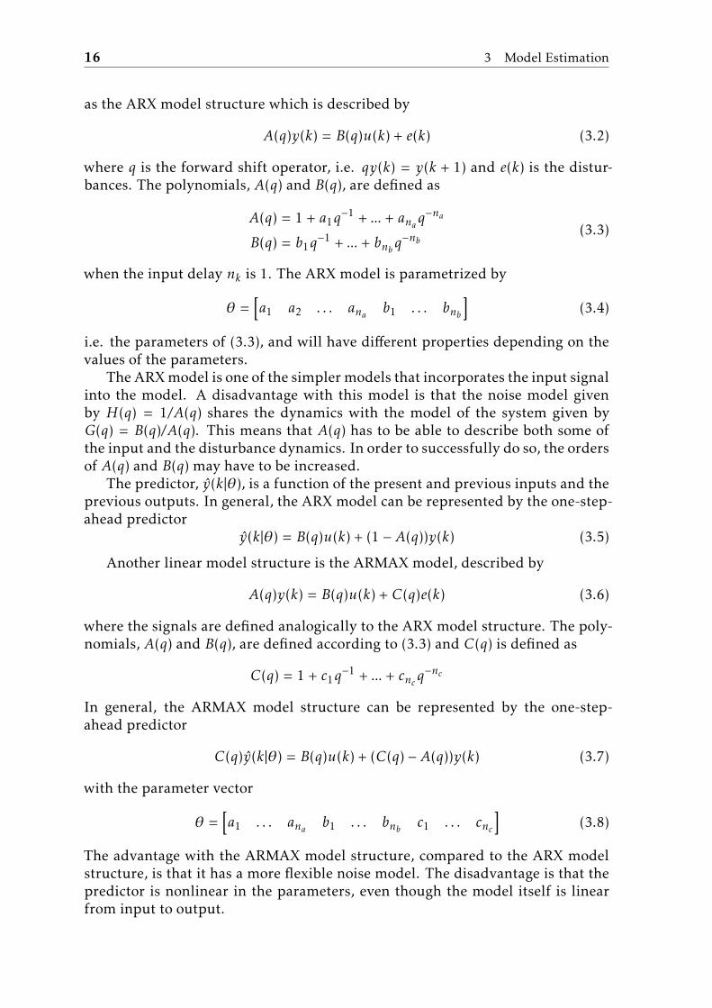
as the ARX model structure which is described by

A(q)y(k) = B(q)u(k) + e(k) (3.2)

where q is the forward shift operator, i.e. qy(k) = y(k + 1) and e(k) is the distur-bances. The polynomials, A(q) and B(q), are defined as

A(q) = 1 + a1q�1 + ... + anaq

�na

B(q) = b1q�1 + ... + bnb q

�nb(3.3)

when the input delay nk is 1. The ARX model is parametrized by

✓ =ha1 a2 . . . ana b1 . . . bnb

i(3.4)

i.e. the parameters of (3.3), and will have di↵erent properties depending on thevalues of the parameters.

The ARXmodel is one of the simplermodels that incorporates the input signalinto the model. A disadvantage with this model is that the noise model givenby H(q) = 1/A(q) shares the dynamics with the model of the system given byG(q) = B(q)/A(q). This means that A(q) has to be able to describe both some ofthe input and the disturbance dynamics. In order to successfully do so, the ordersof A(q) and B(q) may have to be increased.

The predictor, y(k|✓), is a function of the present and previous inputs and theprevious outputs. In general, the ARX model can be represented by the one-step-ahead predictor

y(k|✓) = B(q)u(k) + (1 � A(q))y(k) (3.5)

Another linear model structure is the ARMAX model, described by

A(q)y(k) = B(q)u(k) + C(q)e(k) (3.6)

where the signals are defined analogically to the ARX model structure. The poly-nomials, A(q) and B(q), are defined according to (3.3) and C(q) is defined as

C(q) = 1 + c1q�1 + ... + cnc q

�nc

In general, the ARMAX model structure can be represented by the one-step-ahead predictor

C(q)y(k|✓) = B(q)u(k) + (C(q) � A(q))y(k) (3.7)

with the parameter vector

✓ =ha1 . . . ana b1 . . . bnb c1 . . . cnc

i(3.8)

The advantage with the ARMAX model structure, compared to the ARX modelstructure, is that it has a more flexible noise model. The disadvantage is that thepredictor is nonlinear in the parameters, even though the model itself is linearfrom input to output.

3.2 Closed-loop System Identification 17

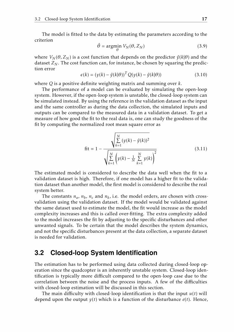
The model is fitted to the data by estimating the parameters according to thecriterion

✓ = argmin✓

VN (✓, ZN ) (3.9)

where VN (✓, ZN ) is a cost function that depends on the predictor y(k|✓) and thedataset ZN . The cost function can, for instance, be chosen by squaring the predic-tion error

✏(k) = (y(k) � y(k|✓))T Q(y(k) � y(k|✓)) (3.10)

where Q is a positive definite weighting matrix and summing over k.The performance of a model can be evaluated by simulating the open-loop

system. However, if the open-loop system is unstable, the closed-loop system canbe simulated instead. By using the reference in the validation dataset as the inputand the same controller as during the data collection, the simulated inputs andoutputs can be compared to the measured data in a validation dataset. To get ameasure of how good the fit to the real data is, one can study the goodness of thefit by computing the normalized root mean square error as

fit = 1 �

sNPk=1

(y(k) � y(k))2

sNPk=1

y(k) � 1

N

NPk=1

y(k)!2

(3.11)

The estimated model is considered to describe the data well when the fit to avalidation dataset is high. Therefore, if one model has a higher fit to the valida-tion dataset than another model, the first model is considered to describe the realsystem better.

The constants na, nb, nc and nk , i.e. the model orders, are chosen with cross-validation using the validation dataset. If the model would be validated againstthe same dataset used to estimate the model, the fit would increase as the modelcomplexity increases and this is called over-fitting. The extra complexity addedto the model increases the fit by adjusting to the specific disturbances and otherunwanted signals. To be certain that the model describes the system dynamics,and not the specific disturbances present at the data collection, a separate datasetis needed for validation.

3.2 Closed-loop System IdentificationThe estimation has to be performed using data collected during closed-loop op-eration since the quadcopter is an inherently unstable system. Closed-loop iden-tification is typically more di�cult compared to the open-loop case due to thecorrelation between the noise and the process inputs. A few of the di�cultieswith closed-loop estimation will be discussed in this section.

The main di�culty with closed-loop identification is that the input u(t) willdepend upon the output y(t) which is a function of the disturbance e(t). Hence,


there is a dependence between the input and the disturbance. This correlationcan lead to a bias in the parameter estimates. However, the bias can be keptsmall if the noise model is flexible enough or if the signal-to-noise ratio is high(Forssell and Ljung, 1999).

There exist several approaches to estimate models from closed-loop data. Oneof these methods is the direct method. In the direct method, a prediction-errorsystem identification method is applied directly as if there was no correlationbetween the input u(t) and the disturbance e(t). It can be seen as the naturalapproach to closed-loop identification but it requires the noise-model to be suf-ficiently rich in order to get consistent estimates. The direct method requires noknowledge about the feedback of the system, no special algorithms or softwareare needed and unstable systems can be handled as long as the output predictoris stable. Since this thesis is focused on estimation of a model of a quadcopter andnot the system identification methods, the direct method will be used straightfor-wardly.

3.3 Data Collection

The data collection was performed outdoors in conditions where the wind wasnot too strong but noticeable. Since the data had to be collected during flight,some sort of controller had to be implemented initially in order for the pilot tobe able to manually control the quadcopter without crashing.

Three PID controllers were implemented on the quadcopter. Two PD con-trollers in roll and pitch and a P controller in yaw. These controllers were tunedto have as weak feedback as possible with low values for the controller parame-ters KP and KD . The data was then collected in a couple of shorter flights, eachlasting about 20-60 s with a sampling time of 0.01s.

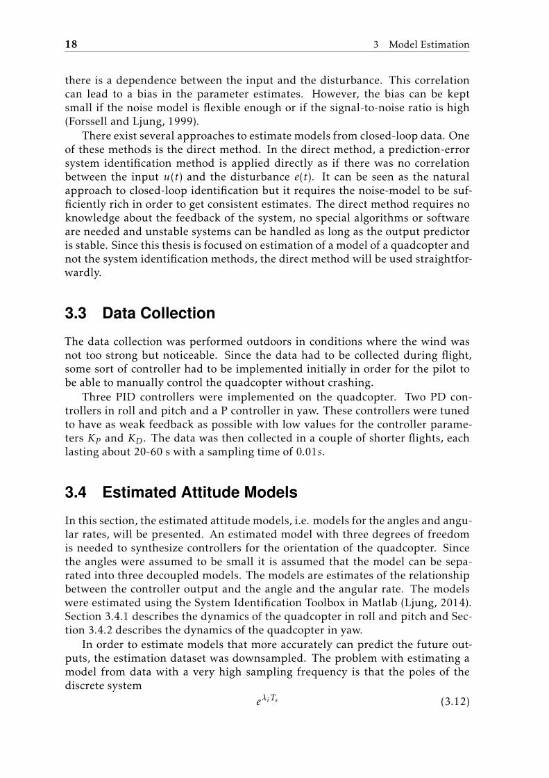
3.4 Estimated Attitude Models

In this section, the estimated attitude models, i.e. models for the angles and angu-lar rates, will be presented. An estimated model with three degrees of freedomis needed to synthesize controllers for the orientation of the quadcopter. Sincethe angles were assumed to be small it is assumed that the model can be sepa-rated into three decoupled models. The models are estimates of the relationshipbetween the controller output and the angle and the angular rate. The modelswere estimated using the System Identification Toolbox in Matlab (Ljung, 2014).Section 3.4.1 describes the dynamics of the quadcopter in roll and pitch and Sec-tion 3.4.2 describes the dynamics of the quadcopter in yaw.

In order to estimate models that more accurately can predict the future out-puts, the estimation dataset was downsampled. The problem with estimating amodel from data with a very high sampling frequency is that the poles of thediscrete system

e�i Ts (3.12)

3.4 Estimated Attitude Models 19

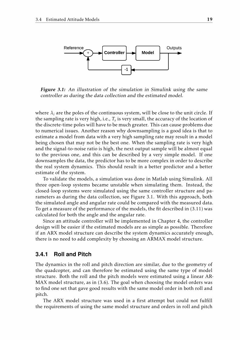
Figure 3.1: An illustration of the simulation in Simulink using the same

controller as during the data collection and the estimated model.

where �i are the poles of the continuous system, will be close to the unit circle. Ifthe sampling rate is very high, i.e., Ts is very small, the accuracy of the location ofthe discrete-time poles will have to be much greater. This can cause problems dueto numerical issues. Another reason why downsampling is a good idea is that toestimate a model from data with a very high sampling rate may result in a modelbeing chosen that may not be the best one. When the sampling rate is very highand the signal-to-noise ratio is high, the next output sample will be almost equalto the previous one, and this can be described by a very simple model. If onedownsamples the data, the predictor has to be more complex in order to describethe real system dynamics. This should result in a better predictor and a betterestimate of the system.

To validate the models, a simulation was done in Matlab using Simulink. Allthree open-loop systems became unstable when simulating them. Instead, theclosed-loop systems were simulated using the same controller structure and pa-rameters as during the data collection, see Figure 3.1. With this approach, boththe simulated angle and angular rate could be compared with the measured data.To get a measure of the performance of the models, the fit described in (3.11) wascalculated for both the angle and the angular rate.

Since an attitude controller will be implemented in Chapter 4, the controllerdesign will be easier if the estimated models are as simple as possible. Thereforeif an ARX model structure can describe the system dynamics accurately enough,there is no need to add complexity by choosing an ARMAX model structure.

3.4.1 Roll and Pitch

The dynamics in the roll and pitch direction are similar, due to the geometry ofthe quadcopter, and can therefore be estimated using the same type of modelstructure. Both the roll and the pitch models were estimated using a linear AR-MAX model structure, as in (3.6). The goal when choosing the model orders wasto find one set that gave good results with the same model order in both roll andpitch.

The ARX model structure was used in a first attempt but could not fulfillthe requirements of using the same model structure and orders in roll and pitch


680 690 700 710 720−1

−0.5

0

0.5

1Angle

680 690 700 710 720−4

−2

0

2

4Angular Rate

675 680 685 690 695 700 705 710 715 720−0.05

0

0.05Control Signal

Roll

Time (seconds)

Am

plit

ud

e

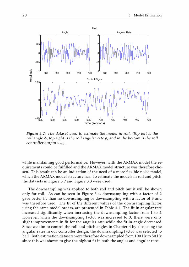
Figure 3.2: The dataset used to estimate the model in roll. Top left is the

roll angle �, top right is the roll angular rate p, and in the bottom is the roll

controller output uroll

.

while maintaining good performance. However, with the ARMAX model the re-quirements could be fulfilled and the ARMAXmodel structure was therefore cho-sen. This result can be an indication of the need of a more flexible noise model,which the ARMAX model structure has. To estimate the models in roll and pitch,the datasets in Figure 3.2 and Figure 3.3 were used.

The downsampling was applied to both roll and pitch but it will be shownonly for roll. As can be seen in Figure 3.4, downsampling with a factor of 2gave better fit than no downsampling or downsampling with a factor of 3 andwas therefore used. The fit of the di↵erent values of the downsampling factor,using the same model orders, are presented in Table 3.1. The fit in angular rateincreased significantly when increasing the downsampling factor from 1 to 2.However, when the downsampling factor was increased to 3, there were onlyslight improvements in fit for the angular rate while the fit in angle decreased.Since we aim to control the roll and pitch angles in Chapter 4 by also using theangular rates in our controller design, the downsampling factor was selected tobe 2. Both estimation datasets were therefore downsampled from 100Hz to 50Hzsince this was shown to give the highest fit in both the angles and angular rates.


680 690 700 710 720−1

−0.5

0

0.5

1Angle

680 690 700 710 720−3

−2

−1

0

1

2

3Angular Rate

675 680 685 690 695 700 705 710 715 720−0.06

−0.04

−0.02

0

0.02

0.04Control Signal

Pitch

Time (seconds)

Am

plit

ud

e

Figure 3.3: The dataset used to estimate the model in pitch. Top left is the

pitch angle ✓, top right is the pitch angular rate q, and in the bottom is the

pitch controller output upitch

.

Table 3.1: The fit of the roll model to the validation data for di↵erent valuesof the downsampling factor on the estimation dataset.

Factor Fit of � Fit of p1 0.4250 0.03372 0.5000 0.47453 0.5139 0.4697

The model orders

na ="3 44 4

#, nb =

"22

#, nc =

"11

#and nk =

"11

#(3.13)

were proven to be the best for both the roll and the pitch model. The model forroll is

A�(z)y�(t) = �A2(z)yp(t) + B�(z)u(t) + C�(z)e�(t)

Ap(z)yp(t) = �A1(z)y�(t) + Bp(z)u(t) + Cp(z)ep(t)(3.14)


500 1000 1500 2000 2500 3000 3500−0.1

0

0.1

0.2

Time (ms)

Angle

(ra

d)

500 1000 1500 2000 2500 3000 3500

−0.5

0

0.5

Time (ms)

Angula

r R

ate

(ra

d/s

)

500 1000 1500 2000 2500 3000 3500

−0.02

0

0.02

0.04

Time (ms)

Contr

ol S

ignal (

−)

Figure 3.4: A plot of the error between the simulated data using the esti-

mated model and the measured signals. Black represents the simulated data

from a model estimated using a downsampling factor of 1 on the estimation

dataset, blue a downsampling factor of 2 and green a downsampling factor

of 3.

where y�(t) is the roll angle, yp(t) is the roll angular rate, the polynomials are ofthe form

Ax(z) = a0 + a1z�1 + a2z

�2 + a3z�3 + a4z

�4 (3.15)

Bx(z) = b1z�1 + b2z

�2 (3.16)

andCx(z) = c0 + c1z

�1 (3.17)

The estimated parameters are given in Tables 3.2 and 3.3,Using this model, the simulation result for the validation data is shown in Fig-

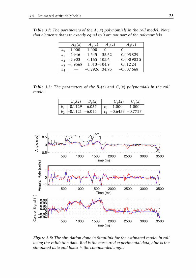
ure 3.5. In this simulation, the fit was 0.5000 for y�(t) and 0.4745 for yp(t). Ascan be seen, the simulated signals follow the measured signals very well. How-ever, in roll angle there is a clear error between the commanded reference andboth the measured and simulated angles. This error is mainly the result of a poorcontroller but also of a disturbance present during the data collection. The con-troller did not have enough gain to accurately follow the reference and the sidewind enlarged the error even more.


Table 3.2: The parameters of the Ax(z) polynomials in the roll model. Note

that elements that are exactly equal to 0 are not part of the polynomials.

A�(z) Ap(z) A1(z) A2(z)a0 1.000 1.000 0 0a1 �2.946 �1.545 �35.62 �0.003 829a2 2.903 �0.165 105.6 �0.000 982 5a3 �0.9568 1.013�104.9 0.012 24a4 — �0.2926 34.95 �0.007 668

Table 3.3: The parameters of the Bx(z) and Cx(z) polynomials in the roll

model.

B�(z) Bp(z) C�(z) Cp(z)b1 0.1129 6.037 c0 1.000 1.000b2 �0.1121 �6.015 c1 �0.6433 �0.7727

500 1000 1500 2000 2500 3000 3500−0.5

0

0.5

Time (ms)

Angle

(ra

d)

500 1000 1500 2000 2500 3000 3500−1

0

1

Time (ms)

Angula

r R

ate

(ra

d/s

)

500 1000 1500 2000 2500 3000 3500−0.04−0.02

00.020.040.060.08

Time (ms)

Contr

ol S

ignal (

−)

Figure 3.5: The simulation done in Simulink for the estimated model in roll

using the validation data. Red is the measured experimental data, blue is the

simulated data and black is the commanded angle.


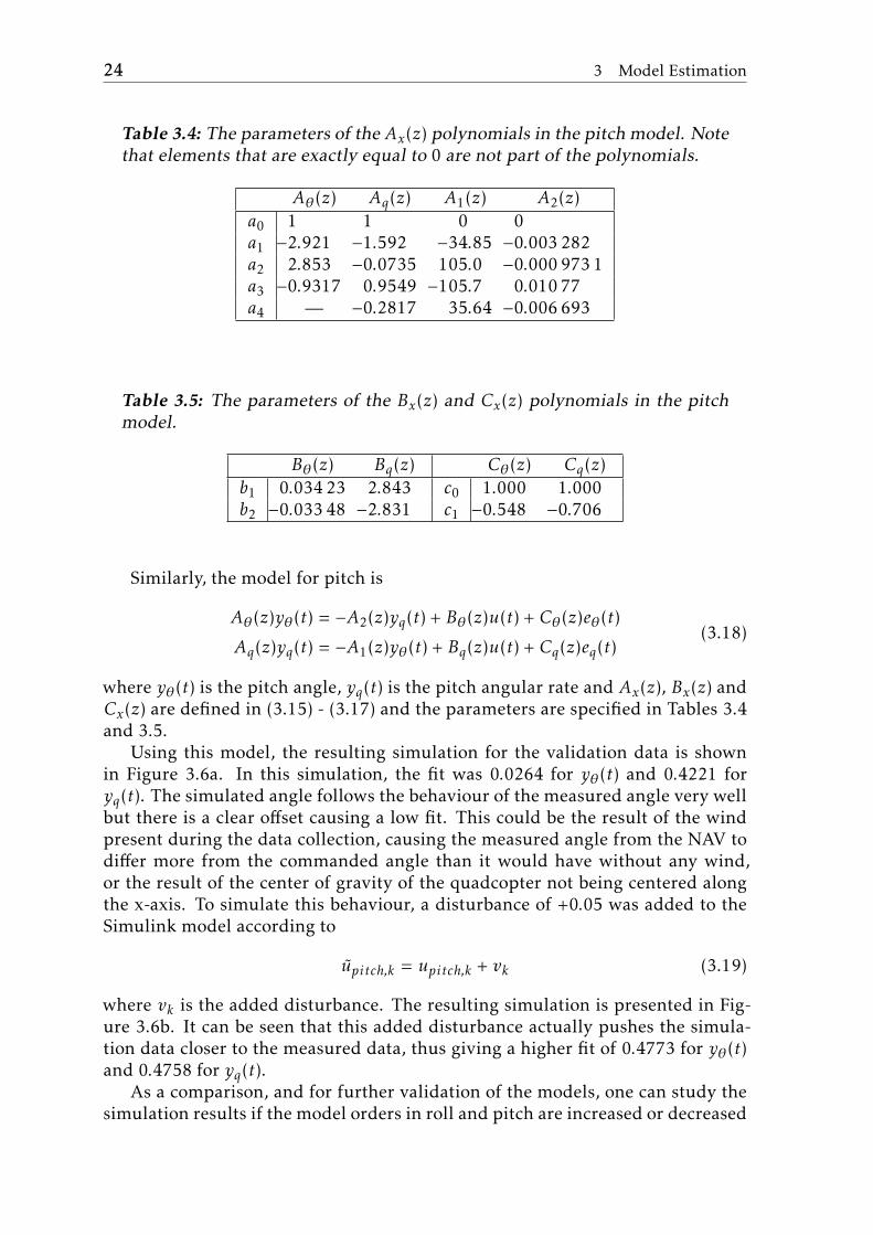
Table 3.4: The parameters of the Ax(z) polynomials in the pitch model. Note


A✓(z) Aq(z) A1(z) A2(z)a0 1 1 0 0a1 �2.921 �1.592 �34.85 �0.003 282a2 2.853 �0.0735 105.0 �0.000 973 1a3 �0.9317 0.9549 �105.7 0.010 77a4 — �0.2817 35.64 �0.006 693

Table 3.5: The parameters of the Bx(z) and Cx(z) polynomials in the pitch

model.

B✓(z) Bq(z) C✓(z) Cq(z)b1 0.034 23 2.843 c0 1.000 1.000b2 �0.033 48 �2.831 c1 �0.548 �0.706

Similarly, the model for pitch is

A✓(z)y✓(t) = �A2(z)yq(t) + B✓(z)u(t) + C✓(z)e✓(t)

Aq(z)yq(t) = �A1(z)y✓(t) + Bq(z)u(t) + Cq(z)eq(t)(3.18)

where y✓(t) is the pitch angle, yq(t) is the pitch angular rate and Ax(z), Bx(z) andCx(z) are defined in (3.15) - (3.17) and the parameters are specified in Tables 3.4and 3.5.

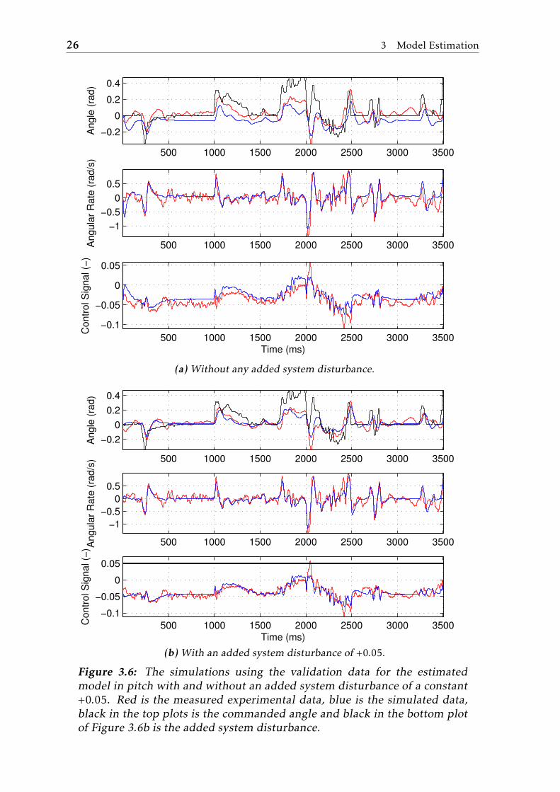
Using this model, the resulting simulation for the validation data is shownin Figure 3.6a. In this simulation, the fit was 0.0264 for y✓(t) and 0.4221 foryq(t). The simulated angle follows the behaviour of the measured angle very wellbut there is a clear o↵set causing a low fit. This could be the result of the windpresent during the data collection, causing the measured angle from the NAV todi↵er more from the commanded angle than it would have without any wind,or the result of the center of gravity of the quadcopter not being centered alongthe x-axis. To simulate this behaviour, a disturbance of +0.05 was added to theSimulink model according to

upitch,k = upitch,k + vk (3.19)

where vk is the added disturbance. The resulting simulation is presented in Fig-ure 3.6b. It can be seen that this added disturbance actually pushes the simula-tion data closer to the measured data, thus giving a higher fit of 0.4773 for y✓(t)and 0.4758 for yq(t).

As a comparison, and for further validation of the models, one can study thesimulation results if the model orders in roll and pitch are increased or decreased


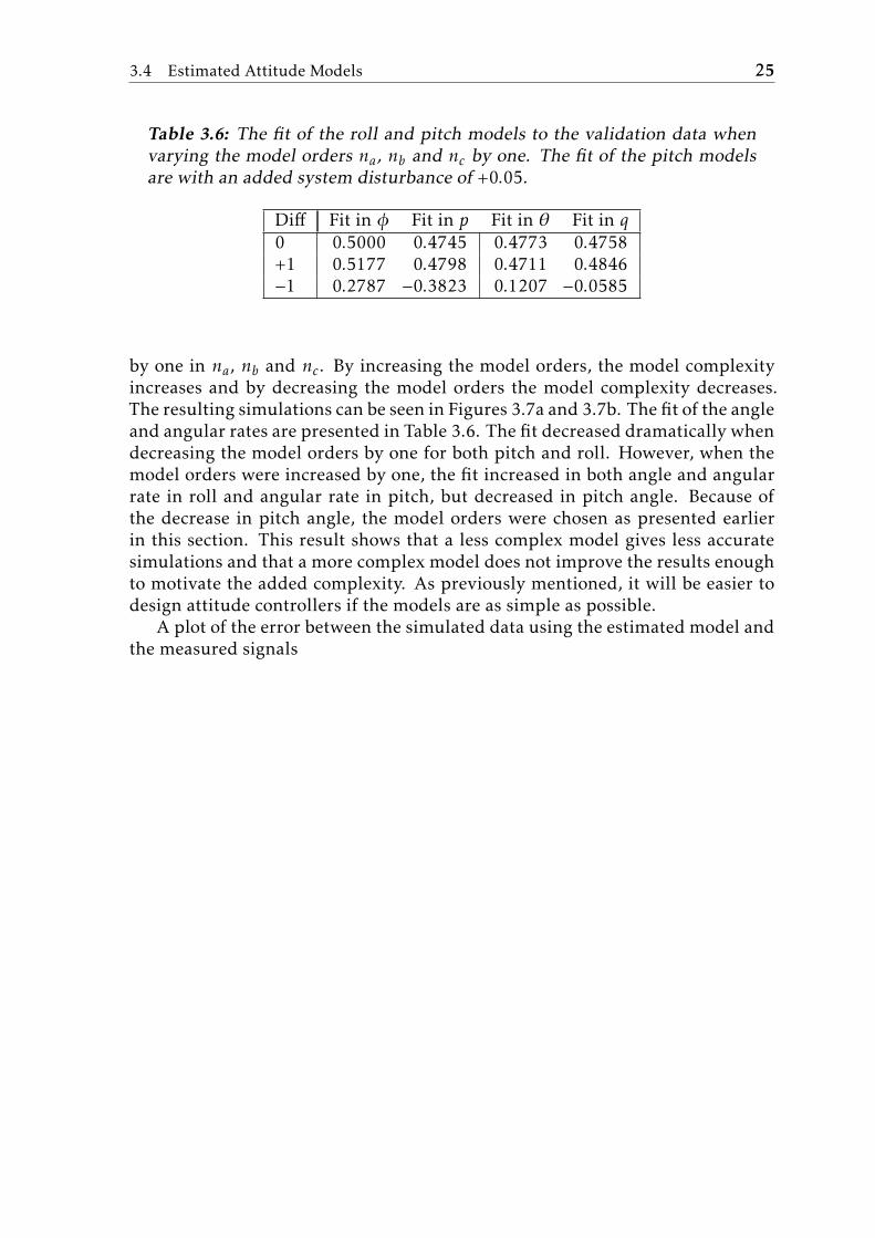
Table 3.6: The fit of the roll and pitch models to the validation data when

varying the model orders na, nb and nc by one. The fit of the pitch models

are with an added system disturbance of +0.05.

Di↵ Fit in � Fit in p Fit in ✓ Fit in q0 0.5000 0.4745 0.4773 0.4758+1 0.5177 0.4798 0.4711 0.4846�1 0.2787 �0.3823 0.1207 �0.0585

by one in na, nb and nc. By increasing the model orders, the model complexityincreases and by decreasing the model orders the model complexity decreases.The resulting simulations can be seen in Figures 3.7a and 3.7b. The fit of the angleand angular rates are presented in Table 3.6. The fit decreased dramatically whendecreasing the model orders by one for both pitch and roll. However, when themodel orders were increased by one, the fit increased in both angle and angularrate in roll and angular rate in pitch, but decreased in pitch angle. Because ofthe decrease in pitch angle, the model orders were chosen as presented earlierin this section. This result shows that a less complex model gives less accuratesimulations and that a more complex model does not improve the results enoughto motivate the added complexity. As previously mentioned, it will be easier todesign attitude controllers if the models are as simple as possible.

A plot of the error between the simulated data using the estimated model andthe measured signals


500 1000 1500 2000 2500 3000 3500

−0.2

0

0.2

0.4A

ngle

(ra

d)

500 1000 1500 2000 2500 3000 3500

−1

−0.5

0

0.5

Angula

r R

ate

(ra

d/s

)

500 1000 1500 2000 2500 3000 3500

−0.1

−0.05

0

0.05

Time (ms)

Contr

ol S

ignal (

−)

(a)Without any added system disturbance.

500 1000 1500 2000 2500 3000 3500

−0.2

0

0.2

0.4

Angle

(ra

d)

500 1000 1500 2000 2500 3000 3500

−1

−0.5

0

0.5

Angula

r R

ate

(ra

d/s

)

500 1000 1500 2000 2500 3000 3500−0.1

−0.05

0

0.05

Time (ms)

Contr

ol S

ignal (

−)

(b)With an added system disturbance of +0.05.

Figure 3.6: The simulations using the validation data for the estimated

model in pitch with and without an added system disturbance of a constant

+0.05. Red is the measured experimental data, blue is the simulated data,

black in the top plots is the commanded angle and black in the bottom plot

of Figure 3.6b is the added system disturbance.


500 1000 1500 2000 2500 3000 3500−0.2

0

0.2A

ng

le (

rad

)

500 1000 1500 2000 2500 3000 3500

−1

0

1

An

gu

lar

Ra

te (

rad

/s)

500 1000 1500 2000 2500 3000 3500

−0.05

0

0.05

Time (ms)

Co

ntr

ol S

ign

al (

−)

(a) Roll

500 1000 1500 2000 2500 3000 3500

−0.2

0

0.2

Angle

(ra

d)

500 1000 1500 2000 2500 3000 3500−1

0

1

Angula

r R

ate

(ra

d/s

)

500 1000 1500 2000 2500 3000 3500

−0.05

0

0.05

Time (ms)

Contr

ol S

ignal (

−)

(b) Pitch

Figure 3.7: A comparison of di↵erent model orders using the validation data.

The plots show the error between the simulated and the measured data.

Blue is the error when using the chosen model orders, green when the model

orders are reduced by 1 and black when the model orders are increased by 1.


3.4.2 YawThe dynamics in yaw was estimated using a linear ARX model structure. Thechoice of using an ARXmodel was due its simplicity and the ARXmodel was seento performwell. Therefore an ARMAXmodel was never tested. The experimentaldata that was used for the model estimation is shown in Figure 3.9. Since we laterin Chapter 4 aim to control the yaw angular rate, and not the angle, we will focusonly on the fit to the angular rate data.

The estimation dataset was downsampled to 33 Hz instead of 100 Hz, corre-sponding to a downsampling factor of 3. This was shown to give the highest fit ofthe angular rate. As can be seen in Figure 3.8, downsampling with a factor of 3 in-dicated better prediction results than both 2 and 4 and was therefore chosen. Thefit of the di↵erent values of the downsampling factor are presented in Table 3.7.As can be seen here, the fit in angular rate increased when increasing the down-sampling factor from 2 to 3. However, as the downsampling factor was increasedto 4 the fit in angular rate decreased slightly. Therefore, the downsampling factorwas set to be 3.

Using simulation as the validation method, the model order

na ="4 43 4

#, nb =

"21

#and nk =

"11

#(3.20)

was proven to be the best for the yaw model. The model is

A (z)y (t) = �A2(z)yr (t) + B (z)u(t) + e (t)

Ar (z)yr (t) = �A1(z)y (t) + Br (z)u(t) + er (t)(3.21)

where y (t) is the yaw angle, yr (t) is the yaw angular rate and Ax(z) and Bx(z)are polynomials, see (3.15) and (3.16), with the parameters given in Tables 3.8and 3.9.

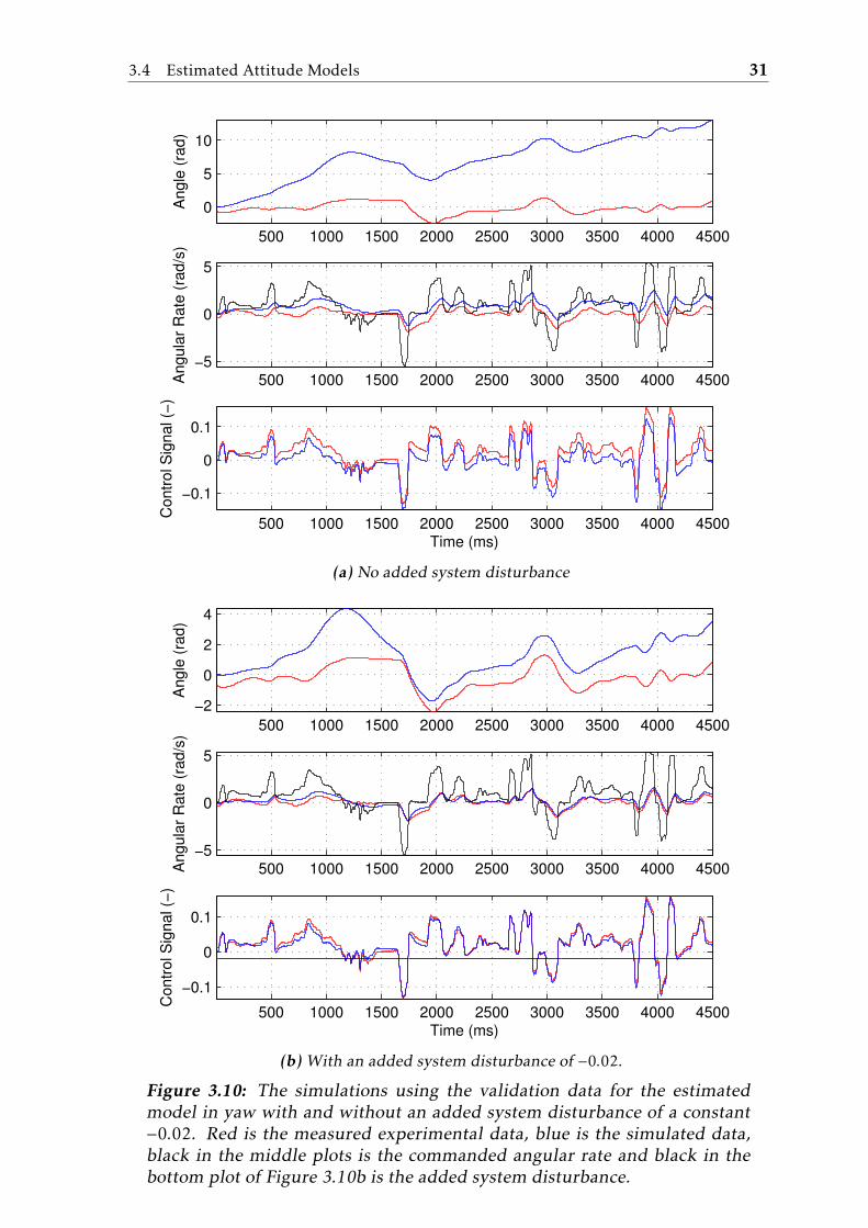
Using (3.21), the resulting simulation for validation data is shown in Fig-ure 3.10a. In this simulation, the fit was �0.4916 for yr (t). Same as when studyingthe simulation results in pitch, it can be seen in Figure 3.10a that the simulatedangular rate follows the trends of the measured angle very well but that there is aclear o↵set causing a low fit. By adding a system disturbance of a constant �0.02,according to

uyaw,k = uyaw,k + vk (3.22)

where vk is the added disturbance, the fit increased to 0.5321 for yr (t). Simulationresults with this disturbance are shown in Figure 3.10b.


500 1000 1500 2000 2500 3000 3500 4000 4500

0

2

4A

ngle

(ra

d)

500 1000 1500 2000 2500 3000 3500 4000 4500−0.5

0

0.5

Angula

r R

ate

(ra

d/s

)

500 1000 1500 2000 2500 3000 3500 4000 4500

−0.01

0

0.01

Time (ms)

Contr

ol S

ignal (

−)

Figure 3.8: A comparison of di↵erent values of the downsampling factor.

The plot shows the error between the simulated data using the estimated

model and the measured data. Black represents the error between the simu-

lated data and themeasured data when themodel is estimated using a down-

sampling factor of 2, blue a downsampling factor of 3 and green a downsam-

pling factor of 4.

Table 3.7: The fit of the yaw model to the validation data for di↵erent valuesof the downsampling factor on the estimation dataset.

Factor Fit of r2 0.65503 0.68664 0.6680


680 690 700 710 720−1

−0.5

0

0.5

1

1.5navpsi

680 690 700 710 720−1

−0.5

0

0.5

1navr

675 680 685 690 695 700 705 710 715 720−0.06

−0.04

−0.02

0

0.02

0.04

0.06uyaw

Yaw

Time (seconds)

Am

plit

ud

e

Figure 3.9: The dataset used to estimate the yaw model. Top left is the yaw

angle , top right is the yaw angular rate r and in the bottom is the yaw

controller output uyaw

.

Table 3.8: The parameters of the Ax(z) polynomials in the yaw model. Note


A (z) Ar (z) A1(z) A2(z)a0 1.000 1.000 0 0a1 �2.753 �1.743 �0.6279 �0.007 034a2 2.665 0.7582 1.188 0.009 113a3 �1.062 0.266 �0.562 �0.004 711a4 0.1504 �0.2676 — 0.002 415

Table 3.9: The parameters of the Bx(z) polynomials in the yaw model. Note


B (z) Br (z)b1 0.028 06 0.3664b2 �0.0255 0


500 1000 1500 2000 2500 3000 3500 4000 4500

0

5

10

Angle

(ra

d)

500 1000 1500 2000 2500 3000 3500 4000 4500−5

0

5

Angula

r R

ate

(ra

d/s

)

500 1000 1500 2000 2500 3000 3500 4000 4500

−0.1

0

0.1

Time (ms)

Contr

ol S

ignal (

−)

(a) No added system disturbance

500 1000 1500 2000 2500 3000 3500 4000 4500−2

0

2

4

Angle

(ra

d)

500 1000 1500 2000 2500 3000 3500 4000 4500−5

0

5

Angula

r R

ate

(ra

d/s

)

500 1000 1500 2000 2500 3000 3500 4000 4500

−0.1

0

0.1

Time (ms)

Contr

ol S

ignal (

−)

(b)With an added system disturbance of �0.02.Figure 3.10: The simulations using the validation data for the estimated

model in yaw with and without an added system disturbance of a constant

�0.02. Red is the measured experimental data, blue is the simulated data,

black in the middle plots is the commanded angular rate and black in the

bottom plot of Figure 3.10b is the added system disturbance.

4Control Design

A control system uses sensor measurements to give feedback to the inputs of thesystem in order to make corrections to achieve a desired performance. A systemthat uses feedback from sensor measurements to compute the inputs is referredto as a closed-loop system. A system that does not is referred to as an open-loopsystem.

This chapter begins with an overview of some control basics. Next, the designof the attitude controller will be explained and presented. Finally, the results andperformance of the controller will be discussed.

4.1 Feedback Control

This section will cover some linear control theory. A general control loop is il-lustrated in Figure 4.1, where G(s) is the plant, i.e. the real physical system ora set of equations describing the system dynamics and Fr (s) and Fy(s) are theparametrized linear controllers.

From Figure 4.1 the closed-loop transfer function

Gc(s) =Fr (s)G(s)

1 + Fy(s)G(s)(4.1)

describing the relationship between the reference r(t) and the output y(t) can bederived. If Fr (s) and Fy(s) are chosen to be equal then

Gc(s) =F(s)G(s)

1 + F(s)G(s)(4.2)

follows from (4.1).

33

34 4 Control Design

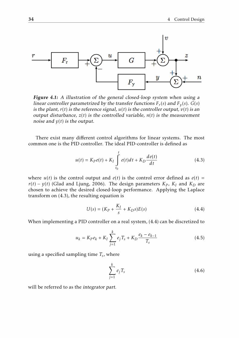
Figure 4.1: A illustration of the general closed-loop system when using a

linear controller parametrized by the transfer functions Fr (s) and Fy(s). G(s)is the plant, r(t) is the reference signal, u(t) is the controller output, v(t) is anoutput disturbance, z(t) is the controlled variable, n(t) is the measurement

noise and y(t) is the output.

There exist many di↵erent control algorithms for linear systems. The mostcommon one is the PID controller. The ideal PID-controller is defined as

u(t) = KPe(t) + KI

tZ

t0

e(t)dt + KDde(t)dt

(4.3)

where u(t) is the control output and e(t) is the control error defined as e(t) =r(t) � y(t) (Glad and Ljung, 2006). The design parameters KP , KI and KD arechosen to achieve the desired closed-loop performance. Applying the Laplacetransform on (4.3), the resulting equation is

U(s) = (KP +KI

s+ KDs)E(s) (4.4)

When implementing a PID controller on a real system, (4.4) can be discretized to

uk = KPek + KI

kX

j=1

ejTs + KDek � ek�1

Ts(4.5)

using a specified sampling time Ts, where

kX

j=1

ejTs (4.6)

will be referred to as the integrator part.

4.2 Implementation Aspects 35

4.2 Implementation AspectsTo implement the controllers on the quadcopter and to guarantee a safe flight,some practical issues had to be solved. First, conditional integration was imple-mented according to Algorithm 1 in order to avoid windup. See Åström (2006)for more information about windup and conditional integration. In Algorithm 1,Ts is the sampling time, uthrottle, uroll, upitch and uyaw are the controller outputsand iroll, ipitch and iyaw are the integrator parts in (4.6). The sum of the absolutevalues of the controller outputs are compared to 1, which is the maximum mo-tor signal an ESC can handle, see (2.21). If the sum is less than 1, the integratorparts are updated. If the sum is greater or equal to 1, the integrator parts are notupdated and stays the same as in the previous iteration. Since the sum of the con-troller outputs, and not the motor signals, are compared to 1, this algorithm issimplified. However, this solution prevents the integrator parts from increasingwhen the motors are saturated in most cases.

Next, since the motor signal that the ESCs can deliver to the motors is lim-ited, a prioritization of the controller outputs was done according to Algorithm 2,where u is a vector containing uthrottle, uroll, upitch and uyaw. According to Sec-tion 2.3 the motor signals are in the range of 0 to 1 and Algorithm 2 prioritizesthe controller outputs and prevents the controller outputs from giving negativemotor signals. For example, if uthrottle is 0.4 then according to (2.21) M1, M2, M3and M4 will all have an output contribution of 0.4 from this controller output. Ifnow uroll is set to 0.5 and upitch = uyaw = 0 then (2.21) gives the outputs to theESCs as M1 = �0.1, M2 = �0.1, M3 = 0.9 and M4 = 0.9. In this case, Algorithm 2will limit uroll and therefore preventing M1 and M2 from getting negative values.The outputs are being prioritized in the order; roll, pitch and last yaw, since thecontrol in roll and pitch are more crucial than yaw to keep the quadcopter stable.Algorithm 2 is simplified due to only taking the controller outputs, and not themotor signals, into account. However, most cases of saturation will be taken careof.

Algorithm 1 Anti Windup Solution

1: if |uthrottle| + |uroll| + |upitch| + |uyaw| < 1 then2: iroll(k + 1) = iroll(k) + Ts(rroll(k) � �(k)).3: ipitch(k + 1) = ipitch(k) + Ts(rpitch(k) � ✓(k)).4: iyaw(k + 1) = iyaw(k) + Ts(ryaw(k) � r(k)).

Algorithm 2 Output Prioritization

1: c = 0.5 � |uthrottle � 0.5|2: for i = 2 : 4 do3: u(i) = max(�c),min(u(i), c))4: c = c � |u(i)|

36 4 Control Design

Algorithm 3 Keep Integrators Deactivated During the Initial Stages of Takeo↵1: if uthrottle(k) < 0.3 then2: iroll(k + 1) = 0.3: ipitch(k + 1) = 0.4: iyaw(k + 1) = 0.

Another important implementation aspect is how to turn on and o↵ the in-tegral action during flight. Since a small error in attitude when in the startingposition will keep integrating, the integral action could potentially cause prob-lems during takeo↵. Once the quadcopter actually lifts o↵, it is possible that theintegrator parts have become very large, which could cause stability problems.To avoid this problem, one can either manually switch on the integrators duringflight, once safely o↵ the ground. This solution requires the integrator parts toalso be reset when switched on. Another solution, which is the one implementedon the quadcopter according to Algorithm 3, is to keep the integrators switchedo↵ until the throttle reaches a certain limit. This allows the integrators to func-tion as planned without needing the pilot’s action. If the throttle is greater than0.3 the integrator parts will update according to Algorithm 1, but if the throttleis less than 0.3 the integrator parts will be set to zero. While in hovering, theneeded throttle is about 0.6-0.7. This means that the throttle will rarely be lessthan 0.3 during flight. Therefore, the algorithm allows the integrators to updatenormally as soon as possible but keeps them at zero until takeo↵.

The algorithms have been implemented in Matlab and translated to C-codewith the Matlab Coder software.

4.3 Attitude Controller

In order to control the orientation of the quadcopter, an attitude controller hasbeen implemented. The attitude controller consists of three decoupled controllers,a roll controller, a pitch controller and a yaw controller, described in Sections 4.3.1,4.3.2 and 4.3.3, respectively.

To choose the parameters of the three controllers, they were simulated to-gether with the estimated models using di↵erent values on the controller param-eters. As a safety measure, to further validate the controllers, the controllerswere designed to control the estimated models as well as possible while also con-trolling three theoretical models of the real system, supplied by Saab DynamicsAB. The theoretical models are in continuous time and are presented in each sec-tion. These continuous-time models were created by trying to mimic the bodeplots of the estimated models in the frequency range of 5 to 30 rad/s. The con-trollers were then designed using both models which should make the result-ing controllers more robust against uncertainty outside the frequency range 5 to30 rad/s.

4.3 Attitude Controller 37

4.3.1 Roll ControllerFigure 4.2 illustrates the quadcopter’s attitude controller in roll. The theoreticalmodel of the roll dynamics is

y� =15000

s(s + 30)(s + 1)

yp =15000

(s + 30)(s + 1)

(4.7)

and is derived from a motor with a bandwidth of 30 rad/s, an amplification of500 from the motor signals to angular rate, a factor s + 1 corresponding to aweakly attenuated angular rate and a pure integration from angular rate to angle.Figure 4.3 compares the bode plots of the theoretical model and the estimatedmodel. As can be seen, the models share the same crossover frequency but di↵ergreatly in the lower frequencies and some in the higher. As previously mentioned,a more robust controller can be designed by also studying the theoretical model.Using both models, the roll controller was tuned manually to track the referenceusing an as small controller output as possible. The resulting controller parame-ters are presented in Table 4.1.

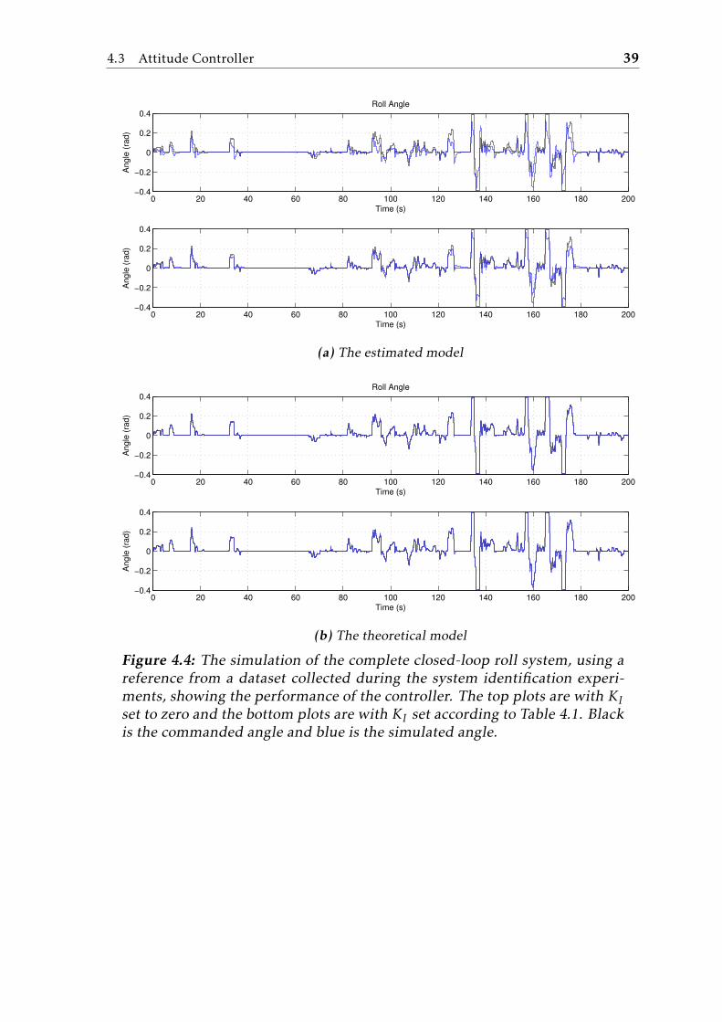
Using the chosen controller parameters, two simulations were performedwithboth models, see Figure 4.4. The first simulations were done with KI set to zero,see the top plots, and the second ones with KI set according to Table 4.1, seethe bottom plots in Figure 4.4. Both simulations are with the closed-loop systemwith the designed controller using a reference from a logged dataset. By simulat-ing the controller with and without KI set to zero, the di↵erence is apparent. Forthe estimated model, the control error is much larger when KI is set to zero andalmost not present with KI not set to zero, except for the larger roll angles wherethe error is still present. For the theoretical model, there is almost no control er-ror, even when KI is zero. It was not possible to achieve better performance withthe estimated model without causing the closed loop system with the theoreticalmodel to become unstable.

Figure 4.2: A illustration of the controller used to control the attitude in roll.

Int is an integrator and G is the quadcopter.

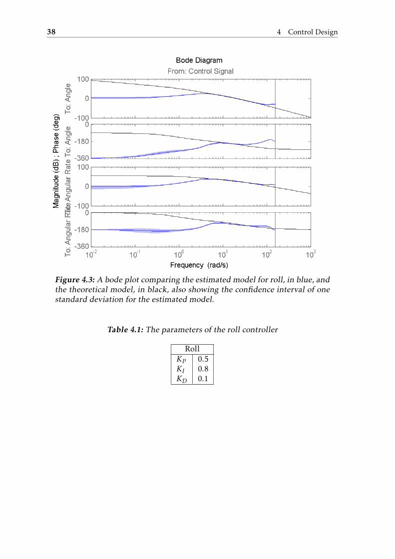
38 4 Control Design

Figure 4.3: A bode plot comparing the estimated model for roll, in blue, and

the theoretical model, in black, also showing the confidence interval of one

standard deviation for the estimated model.

Table 4.1: The parameters of the roll controller

RollKP 0.5KI 0.8KD 0.1


0 20 40 60 80 100 120 140 160 180 200−0.4

−0.2

0

0.2

0.4Roll Angle

Time (s)

An

gle

(ra

d)

0 20 40 60 80 100 120 140 160 180 200−0.4

−0.2

0

0.2

0.4

An

gle

(ra

d)

Time (s)

(a) The estimated model

0 20 40 60 80 100 120 140 160 180 200−0.4

−0.2

0

0.2

0.4Roll Angle

Time (s)

An

gle

(ra

d)

0 20 40 60 80 100 120 140 160 180 200−0.4

−0.2

0

0.2

0.4

An

gle

(ra

d)

Time (s)

(b) The theoretical model

Figure 4.4: The simulation of the complete closed-loop roll system, using a

reference from a dataset collected during the system identification experi-

ments, showing the performance of the controller. The top plots are with KIset to zero and the bottom plots are with KI set according to Table 4.1. Black

is the commanded angle and blue is the simulated angle.

40 4 Control Design

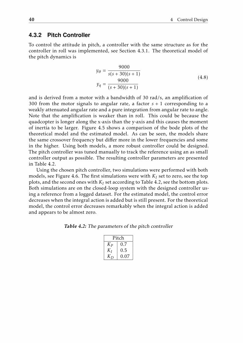
4.3.2 Pitch ControllerTo control the attitude in pitch, a controller with the same structure as for thecontroller in roll was implemented, see Section 4.3.1. The theoretical model ofthe pitch dynamics is

y✓ =9000

s(s + 30)(s + 1)

yq =9000

(s + 30)(s + 1)

(4.8)

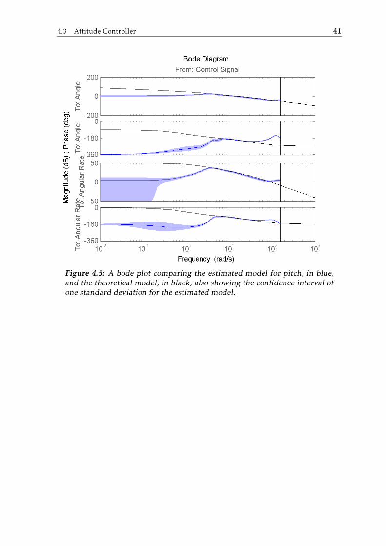
and is derived from a motor with a bandwidth of 30 rad/s, an amplification of300 from the motor signals to angular rate, a factor s + 1 corresponding to aweakly attenuated angular rate and a pure integration from angular rate to angle.Note that the amplification is weaker than in roll. This could be because thequadcopter is longer along the x-axis than the y-axis and this causes the momentof inertia to be larger. Figure 4.5 shows a comparison of the bode plots of thetheoretical model and the estimated model. As can be seen, the models sharethe same crossover frequency but di↵er more in the lower frequencies and somein the higher. Using both models, a more robust controller could be designed.The pitch controller was tuned manually to track the reference using an as smallcontroller output as possible. The resulting controller parameters are presentedin Table 4.2.

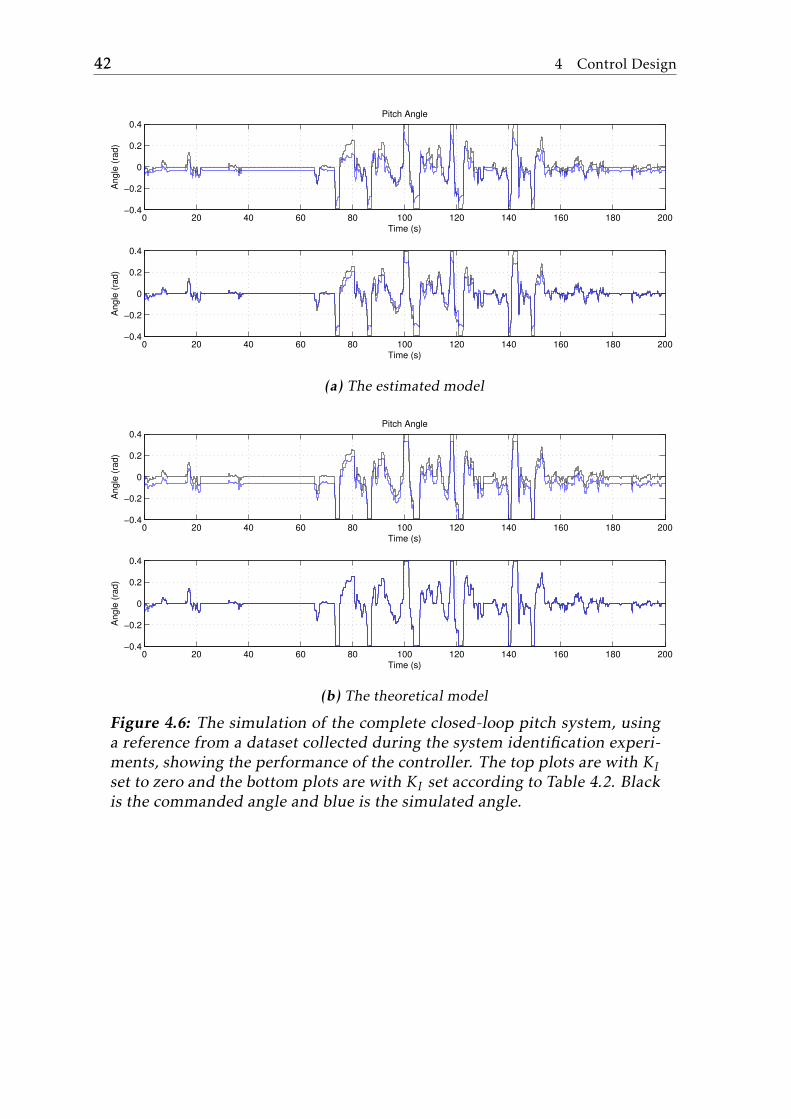
Using the chosen pitch controller, two simulations were performed with bothmodels, see Figure 4.6. The first simulations were with KI set to zero, see the topplots, and the second ones with KI set according to Table 4.2, see the bottom plots.Both simulations are on the closed-loop system with the designed controller us-ing a reference from a logged dataset. For the estimated model, the control errordecreases when the integral action is added but is still present. For the theoreticalmodel, the control error decreases remarkably when the integral action is addedand appears to be almost zero.

Table 4.2: The parameters of the pitch controller

PitchKP 0.7KI 0.5KD 0.07


Figure 4.5: A bode plot comparing the estimated model for pitch, in blue,

and the theoretical model, in black, also showing the confidence interval of

one standard deviation for the estimated model.

42 4 Control Design

0 20 40 60 80 100 120 140 160 180 200−0.4

−0.2

0

0.2

0.4Pitch Angle

Time (s)

An

gle

(ra

d)

0 20 40 60 80 100 120 140 160 180 200−0.4

−0.2

0

0.2

0.4

An

gle

(ra

d)

Time (s)


0 20 40 60 80 100 120 140 160 180 200−0.4

−0.2

0

0.2

0.4Pitch Angle

Time (s)

An

gle

(ra

d)

0 20 40 60 80 100 120 140 160 180 200−0.4

−0.2

0

0.2

0.4

An

gle

(ra

d)

Time (s)


Figure 4.6: The simulation of the complete closed-loop pitch system, using

a reference from a dataset collected during the system identification experi-




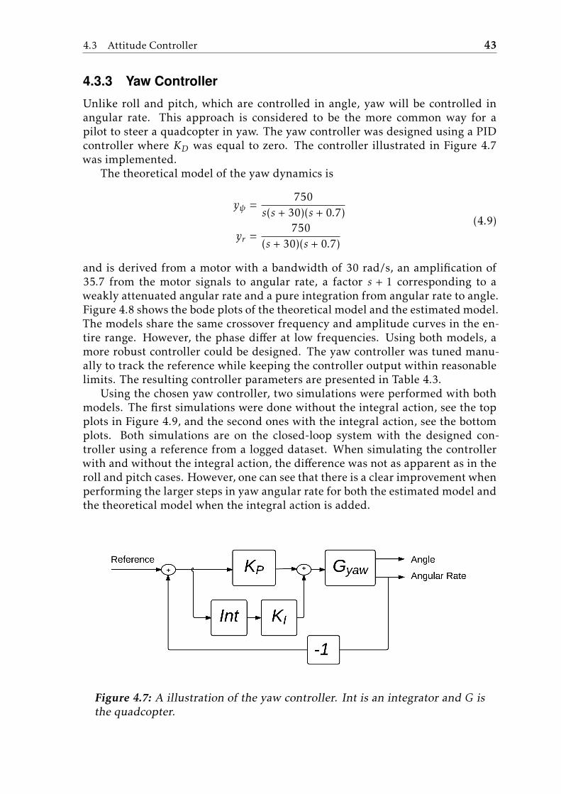
4.3.3 Yaw ControllerUnlike roll and pitch, which are controlled in angle, yaw will be controlled inangular rate. This approach is considered to be the more common way for apilot to steer a quadcopter in yaw. The yaw controller was designed using a PIDcontroller where KD was equal to zero. The controller illustrated in Figure 4.7was implemented.

The theoretical model of the yaw dynamics is

y =750

s(s + 30)(s + 0.7)

yr =750

(s + 30)(s + 0.7)

(4.9)

and is derived from a motor with a bandwidth of 30 rad/s, an amplification of35.7 from the motor signals to angular rate, a factor s + 1 corresponding to aweakly attenuated angular rate and a pure integration from angular rate to angle.Figure 4.8 shows the bode plots of the theoretical model and the estimated model.The models share the same crossover frequency and amplitude curves in the en-tire range. However, the phase di↵er at low frequencies. Using both models, amore robust controller could be designed. The yaw controller was tuned manu-ally to track the reference while keeping the controller output within reasonablelimits. The resulting controller parameters are presented in Table 4.3.

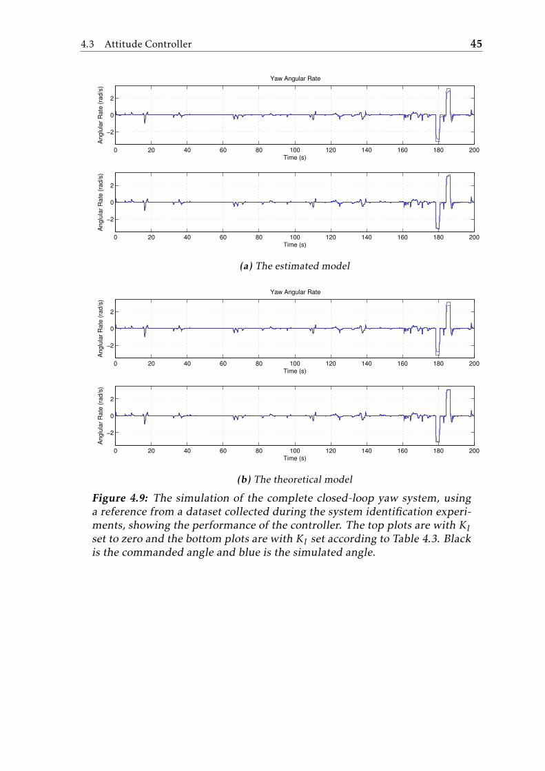
Using the chosen yaw controller, two simulations were performed with bothmodels. The first simulations were done without the integral action, see the topplots in Figure 4.9, and the second ones with the integral action, see the bottomplots. Both simulations are on the closed-loop system with the designed con-troller using a reference from a logged dataset. When simulating the controllerwith and without the integral action, the di↵erence was not as apparent as in theroll and pitch cases. However, one can see that there is a clear improvement whenperforming the larger steps in yaw angular rate for both the estimated model andthe theoretical model when the integral action is added.

Figure 4.7: A illustration of the yaw controller. Int is an integrator and G is

the quadcopter.

44 4 Control Design

Figure 4.8: A bode plot comparing the estimated model for yaw, in blue, and

the theoretical model, in black, also showing the confidence interval of one

standard deviation for the estimated model.

Table 4.3: The parameters of the yaw controller

YawKP 0.2KI 0.2


0 20 40 60 80 100 120 140 160 180 200

−2

0

2

Yaw Angular Rate

Time (s)

An

glu

lar

Ra

te (

rad

/s)

0 20 40 60 80 100 120 140 160 180 200

−2

0

2

An

glu

lar

Ra

te (

rad

/s)

Time (s)


0 20 40 60 80 100 120 140 160 180 200

−2

0

2

Yaw Angular Rate

Time (s)

An

glu

lar

Ra

te (

rad

/s)

0 20 40 60 80 100 120 140 160 180 200

−2

0

2

An

glu

lar

Ra

te (

rad

/s)

Time (s)


Figure 4.9: The simulation of the complete closed-loop yaw system, using

a reference from a dataset collected during the system identification experi-



46 4 Control Design

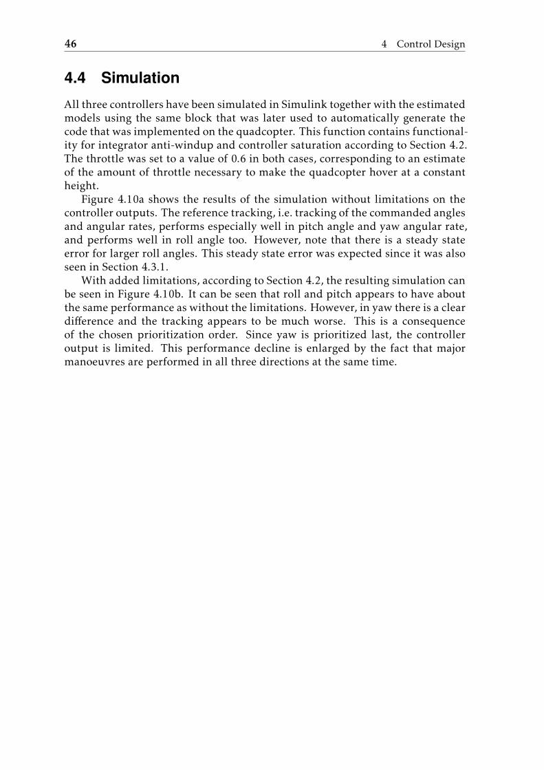
4.4 SimulationAll three controllers have been simulated in Simulink together with the estimatedmodels using the same block that was later used to automatically generate thecode that was implemented on the quadcopter. This function contains functional-ity for integrator anti-windup and controller saturation according to Section 4.2.The throttle was set to a value of 0.6 in both cases, corresponding to an estimateof the amount of throttle necessary to make the quadcopter hover at a constantheight.

Figure 4.10a shows the results of the simulation without limitations on thecontroller outputs. The reference tracking, i.e. tracking of the commanded anglesand angular rates, performs especially well in pitch angle and yaw angular rate,and performs well in roll angle too. However, note that there is a steady stateerror for larger roll angles. This steady state error was expected since it was alsoseen in Section 4.3.1.

With added limitations, according to Section 4.2, the resulting simulation canbe seen in Figure 4.10b. It can be seen that roll and pitch appears to have aboutthe same performance as without the limitations. However, in yaw there is a cleardi↵erence and the tracking appears to be much worse. This is a consequenceof the chosen prioritization order. Since yaw is prioritized last, the controlleroutput is limited. This performance decline is enlarged by the fact that majormanoeuvres are performed in all three directions at the same time.

4.4 Simulation 47

5 10 15 20 25 30 35 40 45

−0.2

0

0.2

0.4

0.6

Roll Angle

Angle

(ra

d)

5 10 15 20 25 30 35 40 45

−0.4

−0.2

0

0.2

Pitch Angle

Angle

(ra

d)

5 10 15 20 25 30 35 40 45

−5

0

5

Yaw Angular Rate

Angula

r R

ate

(ra

d/s

)

Time (s)

(a) No limit on the controller outputs

5 10 15 20 25 30 35 40 45

−0.2

0

0.2

0.4

0.6

Roll Angle

Angle

(ra

d)

5 10 15 20 25 30 35 40 45

−0.4

−0.2

0

0.2

Pitch Angle

Angle

(ra

d)

5 10 15 20 25 30 35 40 45

−5

0

5

Yaw Angular Rate

Angula

r R

ate

(ra

d/s

)

Time (s)

(b)With a limit on the sum of the controller outputs

Figure 4.10: The simulation of the three controllers together with (a) and

without (b) a limit on the sum of the controller outputs. Black is the com-

manded angles and angular rates and blue is the simulated angles and an-

gular rates.

48 4 Control Design

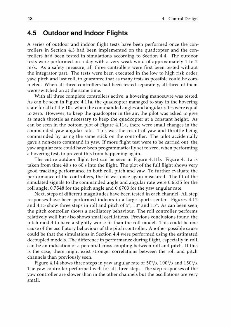
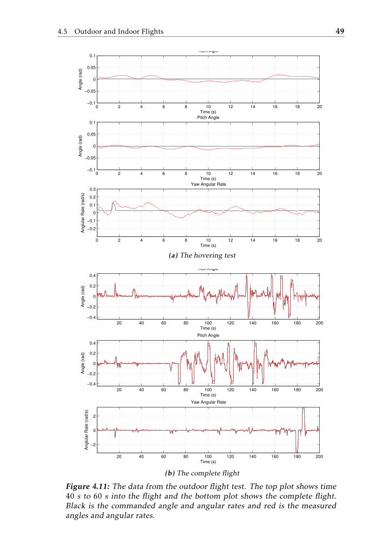
4.5 Outdoor and Indoor FlightsA series of outdoor and indoor flight tests have been performed once the con-trollers in Section 4.3 had been implemented on the quadcopter and the con-trollers had been tested in simulations according to Section 4.4. The outdoortests were performed on a day with a very weak wind of approximately 1 to 2m/s. As a safety measure, all three controllers were first been tested withoutthe integrator part. The tests were been executed in the low to high risk order,yaw, pitch and last roll, to guarantee that as many tests as possible could be com-pleted. When all three controllers had been tested separately, all three of themwere switched on at the same time.

With all three complete controllers active, a hovering manoeuvre was tested.As can be seen in Figure 4.11a, the quadcopter managed to stay in the hoveringstate for all of the 10 s when the commanded angles and angular rates were equalto zero. However, to keep the quadcopter in the air, the pilot was asked to giveas much throttle as necessary to keep the quadcopter at a constant height. Ascan be seen in the bottom plot of Figure 4.11a, there were small changes in thecommanded yaw angular rate. This was the result of yaw and throttle beingcommanded by using the same stick on the controller. The pilot accidentallygave a non-zero command in yaw. If more flight test were to be carried out, theyaw angular rate could have been programmatically set to zero, when performinga hovering test, to prevent this from happening again.

The entire outdoor flight test can be seen in Figure 4.11b. Figure 4.11a istaken from time 40 s to 60 s into the flight. The plot of the full flight shows verygood tracking performance in both roll, pitch and yaw. To further evaluate theperformance of the controllers, the fit was once again measured. The fit of thesimulated signals to the commanded angle and angular rate were 0.6535 for theroll angle, 0.7548 for the pitch angle and 0.6703 for the yaw angular rate.

Next, steps of di↵erent magnitudes have been tested in each channel. All stepresponses have been performed indoors in a large sports center. Figures 4.12and 4.13 show three steps in roll and pitch of 5°, 10° and 15°. As can been seen,the pitch controller shows a oscillatory behaviour. The roll controller performsrelatively well but also shows small oscillations. Previous conclusions found thepitch model to have a slightly worse fit than the roll model. This could be onecause of the oscillatory behaviour of the pitch controller. Another possible causecould be that the simulations in Section 4.4 were performed using the estimateddecoupled models. The di↵erence in performance during flight, especially in roll,can be an indication of a potential cross coupling between roll and pitch. If thisis the case, there might exist stronger correlations between the roll and pitchchannels than previously seen.

Figure 4.14 shows three steps in yaw angular rate of 50°/s, 100°/s and 150°/s.The yaw controller performed well for all three steps. The step responses of theyaw controller are slower than in the other channels but the oscillations are verysmall.

4.5 Outdoor and Indoor Flights 49

0 2 4 6 8 10 12 14 16 18 20−0.1

−0.05

0

0.05

0.1Roll Angle

Angle

(ra

d)

Time (s)

0 2 4 6 8 10 12 14 16 18 20−0.1

−0.05

0

0.05

0.1Pitch Angle

Angle

(ra

d)

Time (s)

0 2 4 6 8 10 12 14 16 18 20

−0.2

−0.1

0

0.1

0.2

0.3Yaw Angular Rate

Time (s)

Anglu

lar

Rate

(ra

d/s

)

(a) The hovering test

20 40 60 80 100 120 140 160 180 200

−0.4

−0.2

0

0.2

0.4

Roll Angle

Angle

(ra

d)

Time (s)

20 40 60 80 100 120 140 160 180 200

−0.4

−0.2

0

0.2

0.4

Pitch Angle

Angle

(ra

d)

Time (s)

20 40 60 80 100 120 140 160 180 200

−2

0

2

Yaw Angular Rate

Time (s)

Anglu

lar

Rate

(ra

d/s

)

(b) The complete flight

Figure 4.11: The data from the outdoor flight test. The top plot shows time

40 s to 60 s into the flight and the bottom plot shows the complete flight.

Black is the commanded angle and angular rates and red is the measured

angles and angular rates.

50 4 Control Design

0.5 1 1.5 2 2.5 30

2

4

5 degA

ngle

(deg)

0.5 1 1.5 2 2.5 3 3.5 40

5

10

10 deg

Angle

(deg)

0.5 1 1.5 2 2.5 30

5

10

15

15 deg

Angle

(deg)

Time (s)

Figure 4.12: The data from the indoor flight test where three steps in roll

were performed. Black is the commanded angle and red is the logged angle.

4.5 Outdoor and Indoor Flights 51

0.5 1 1.5 2 2.5 3 3.5 40

2

4

6

5 deg

Angle

(deg)

0.5 1 1.5 2 2.50

5

10

10 deg

Angle

(deg)

0.5 1 1.5 2 2.5 3 3.50

5

10

15

15 deg

Angle

(deg)

Time (s)

Figure 4.13: The data from the indoor flight test where three steps in pitch

were performed. Black is the commanded angle and red is the logged angle.

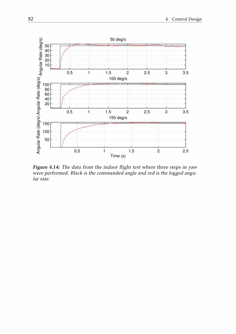
52 4 Control Design

0.5 1 1.5 2 2.5 3 3.5

1020304050

50 deg/sA

ngula

r R

ate

(deg/s

)

0.5 1 1.5 2 2.5 3 3.5

20406080

100

100 deg/s

Angula

r R

ate

(deg/s

)

0.5 1 1.5 2 2.5

50

100

150

150 deg/s

Angula

r R

ate

(deg/s

)

Time (s)

Figure 4.14: The data from the indoor flight test where three steps in yaw

were performed. Black is the commanded angle and red is the logged angu-

lar rate.

5Conclusions and Future Work

In this thesis, black-box models describing the quadcopter system dynamics forattitude control have been estimated using closed-loop data. The models haveshown good simulation performance and they can be used in simulations to prop-erly tune a PID controller for outdoor flight purposes. This chapter gives a sum-mary and a discussion regarding the results presented in Chapter 3 and Chap-ter 4. This is followed by a presentation of ideas for future development.

5.1 Conclusions

The models for the roll and pitch dynamics were forced to have the same modelstructure and orders since this reflects the geometry of the quadcopter. This ap-proach resulted in the need of an ARMAX model structure for the roll and pitchdynamics, instead of an ARX model structure. This could be an indication of theneed for a more flexible noise model. However, the yaw dynamics could be esti-mated with an ARX model structure. The simulation performance was good forall three models but slightly worse for the pitch model.

The estimation datasets were downsampled to make it easier to obtain in-formative model estimates. This resulted in higher fit for all the models. Fur-thermore, although the data collection was performed in closed-loop, the directmethod gave good results.

All three models describing the system dynamics were shown to provide accu-rate enough simulations in order to design the attitude controllers. The attitudecontrollers performed well during the test flights, and were able to control thequadcopter around the hovering state while only requiring the pilot to handle thethrottle to keep the desired altitude. The step responses from the indoor flightsshow that the performance of the roll and yaw controllers are good. However,the performance of the pitch controller could be improved further since there are

53

54 5 Conclusions and Future Work

oscillations present.To conclude, these black-box models and attitude controllers provide a good

foundation for future work on the platform. Some potential ideas are presentedin the next section.

5.2 Future WorkA first improvement would be to include sensors for measuring the longitudi-nal and lateral position as well as the height above ground, for instance, usinga global positioning system (GPS) sensor and an ultrasonic range finder. With aheight measurement, a model could be estimated to describe the throttle dynam-ics. The attitude models and the height model will together describe all of thequadcopter movements. With this complete model and the additional measure-ments, an interesting problem is to implement a position controller, in order toguarantee the quadcopter from drifting sideways and to allow it to hover, withoutany input from a pilot.

With the position controller mentioned above implemented, a second ideais to design a control algorithm to allow for fully autonomous flight, includingautonomous takeo↵ and landing. Once this functionality has been implemented,the possibilities for further development are many.

Another improvement would be to modify Algorithms 1 and 2 in Section 4.2to take the motor signals into account and not only the controller outputs. Withthis modification the performance of the attitude controllers should be improved.

The attitude controllers in this thesis were designed using simulations. An-other interesting improvement would be to use some kind of uncertainty mea-sure of the estimated model, and to use that measure in the controller design toautomate the process of designing more robust controllers when the model un-certainty is higher, and to design a more aggressive controller when the modeluncertainty is lower, according to Section 4.3. This tool would facilitate the con-troller design process and make it more automated.

The final idea is to implement a controller with additional robustness proper-ties. One could, for example, design a controller that is robust towards changesin mass or moment of inertia. With this robust controller implemented, the quad-copter could pick up and drop o↵ objects of unknown weights and shapes. Fur-thermore, it would be interesting to investigate if a less oscillatory controller canbe designed and how the pitch channel influences the roll channel.

Bibliography

Fabio Beltramini, Marco Bergamasco, and Marco Lovera. Experiment designfor MIMO model identification, with application to rotorcraft dynamics. InProceedings of 18th IFAC World Congress, pages 14392–14397, Milano, Italy,2011. Cited on page 2.

Mark Cutler. Design and control of an autonomous variable-pitch quadrotor he-licopter. Master’s thesis, Massachusetts Institute of Technology, Department ofAeronautics and Astronautics, August 2012. Cited on page 1.

Urban Forssell and Lennart Ljung. Closed-loop identification revisited. Auto-

matica, 35(7):1215–1241, July 1999. ISSN 0005-1098. Cited on page 18.

T. Glad and L. Ljung. Modeling of dynamic systems. Prentice Hall, 1995. Citedon page 15.

T. Glad and L. Ljung. Reglerteknik, Grundläggande teori. Studentlitteratur AB,4:7 edition, 2006. ISBN 9789144022758. Cited on page 34.

S. Gupte, P.I.T. Mohandas, and J.M. Conrad. A survey of quadrotor unmannedaerial vehicles. In Southeastcon, 2012 Proceedings of IEEE, pages 1–6, Orlando,FL, USA, March 2012. doi: 10.1109/SECon.2012.6196930. Cited on page 1.

Qianying Li. Grey-box system identification of a quadrotor unmanned aerialvehicle. Master’s thesis, Delft University of Technology, The Netherlands, 2014.Cited on page 2.

Lennart Ljung. System Identification: Theory for the user. PTR Prentice HallInformation and System Sciences Series., 2nd edition, 1999. Cited on page 15.

Lennart Ljung. Black-box models from input-output measurements. In Instru-

mentation and Measurement Technology Conference, 2001. IMTC 2001. Pro-

ceedings of the 18th IEEE, volume 1, pages 138–146 vol.1, May 2001. doi:10.1109/IMTC.2001.928802. Cited on page 2.

Lennart Ljung. System identification toolbox: user’s guide. MathWorks, 2014bedition, 2014. Cited on page 18.

55

56 Bibliography

Z. Mustapa, S. Saat, S.H. Husin, and N. Abas. Altitude controller design for multi-copter UAV. In Computer, Communications, and Control Technology (I4CT),

2014 International Conference on, pages 382–387, Sept 2014. doi: 10.1109/I4CT.2014.6914210. Cited on page 1.

K. Nagarjuna and G.R. Suresh. Design of e↵ective landing mechanism for fullyautonomous unmanned aerial vehicle. In Signal Processing, Communication

and Networking (ICSCN), 2015 3rd International Conference on, pages 1–6,Madras Institute of Technology, Anna University, Chennai, India, March 2015.doi: 10.1109/ICSCN.2015.7219864. Cited on page 1.

J. Nikolic, M. Burri, J. Rehder, S. Leutenegger, C. Huerzeler, and R. Siegwart. AUAV system for inspection of industrial facilities. In Aerospace Conference,

2013 IEEE, pages 1–8, March 2013. doi: 10.1109/AERO.2013.6496959. Citedon page 1.

P. Panizza, F. Riccardi, and M. Lovera. In Workshop on Advanced Control and

Navigation for Autonomous Aeroespace Vehicles, Seville, Italy, June 2015. doi:10.1016/j.ifacol.2015.08.060. Cited on page 2.

S. Thornton and J. Marion. Classical Dynamics of Particles and Systems.Brooks/Cole, Cengage Learning, 2004. ISBN 9780534408961. Cited on page9.

S. Waharte and N. Trigoni. Supporting search and rescue operations with UAVs.In Emerging Security Technologies (EST), 2010 International Conference on,pages 142–147, Sept 2010. doi: 10.1109/EST.2010.31. Cited on page 1.

Yang Yungao, Xian Bin, Yin Qiang, Li Haotao, and Zeng Wei. Current researchsituation of frameworks and control of quadrotor unmanned aerial vehicles. InControl Conference (CCC), 2011 30th Chinese, Shandong, China, 2011. Citedon page 1.

Hanlin Zhang, Sixiao Wei, Wei Yu, E. Blasch, Genshe Chen, Dan Shen, andK. Pham. Scheduling methods for unmanned aerial vehicle based delivery sys-tems. In Digital Avionics Systems Conference (DASC), 2014 IEEE/AIAA 33rd,pages 6C1–1–6C1–9, Oct 2014. doi: 10.1109/DASC.2014.6979499. Cited onpage 1.

Hägglund Tore Åström, Karl J. Advanced PID Control. ISA, 2006. Cited on page35.

black-box modeling and attitude control of a quadcopterabstract in this thesis, black-box models...

Documents