black-box optimization of noisy functions with...
TRANSCRIPT
Black-box optimization of noisy functions withunknown smoothness
Jean-Bastien Grill Michal ValkoSequeL team, INRIA Lille - Nord Europe, France
[email protected] [email protected]
Remi MunosGoogle DeepMind, UK∗
Abstract
We study the problem of black-box optimization of a function f of any dimen-sion, given function evaluations perturbed by noise. The function is assumed tobe locally smooth around one of its global optima, but this smoothness is un-known. Our contribution is an adaptive optimization algorithm, POO or paralleloptimistic optimization, that is able to deal with this setting. POO performs almostas well as the best known algorithms requiring the knowledge of the smoothness.Furthermore, POO works for a larger class of functions than what was previouslyconsidered, especially for functions that are difficult to optimize, in a very precisesense. We provide a finite-time analysis of POO’s performance, which shows thatits error after n evaluations is at most a factor of
√lnn away from the error of the
best known optimization algorithms using the knowledge of the smoothness.
1 Introduction
We treat the problem of optimizing a function f : X → R given a finite budget of n noisy evalua-tions. We consider that the cost of any of these function evaluations is high. That means, we careabout assessing the optimization performance in terms of the sample complexity, i.e., the numberof n function evaluations. This is typically the case when one needs to tune parameters for a complexsystem seen as a black-box, which performance can only be evaluated by a costly simulation. Onesuch example, is the hyper-parameter tuning where the sensitivity to perturbations is large and thederivatives of the objective function with respect to these parameters do not exist or are unknown.
Such setting fits the sequential decision-making setting under bandit feedback. In this setting, theactions are the points that lie in a domain X . At each step t, an algorithm selects an action xt ∈ Xand receives a reward rt, which is a noisy function evaluation such that rt = f(xt) + εt, where εt isa bounded noise with E [εt |xt ] = 0. After n evaluations, the algorithm outputs its best guess x(n),which can be different from xn. The performance measure we want to minimize is the value of thefunction at the returned point compared to the optimum, also referred to as simple regret,
Rn , supx∈X
f(x)− f (x (n)).
We assume there exists at least one point x? ∈ X such that f(x?) = supx∈X f(x).
The relationship with bandit settings motivated UCT [10, 8], an empirically successful heuristicthat hierarchically partitions domain X and selects the next point xt ∈ X using upper confidencebounds [1]. The empirical success of UCT on one side but the absence of performance guarantees forit on the other, incited research on similar but theoretically founded algorithms [4, 9, 12, 2, 6].
As the global optimization of the unknown function without absolutely any assumptions wouldbe a daunting needle-in-a-haystack problem, most of the algorithms assume at least a very weak
∗on the leave from SequeL team, INRIA Lille - Nord Europe, France
1

assumption that the function does not decrease faster than a known rate around one of its globaloptima. In other words, they assume a certain local smoothness property of f . This smoothnessis often expressed in the form of a semi-metric ` that quantifies this regularity [4]. Naturally, thisregularity also influences the guarantees that these algorithms are able to furnish. Many of themdefine a near-optimality dimension d or a zooming dimension. These are `-dependent quantitiesused to bound the simple regret Rn or a related notion called cumulative regret.
Our work focuses on a notion of such near-optimality dimension d that does not directly relatethe smoothness property of f to a specific metric ` but directly to the hierarchical partitioningP = Ph,i, a tree-based representation of the space used by the algorithm. Indeed, an interestingfundamental question is to determine a good characterization of the difficulty of the optimizationfor an algorithm that uses a given hierarchical partitioning of the space X as its input. The kind ofhierarchical partitioning Ph,i we consider is similar to the ones introduced in prior work: for anydepth h ≥ 0 in the tree representation, the set of cells Ph,i1≤i≤Ih form a partition of X , where Ihis the number of cells at depth h. At depth 0, the root of the tree, there is a single cell P0,1 = X . Acell Ph,i of depth h is split into several children subcells Ph+1,jj of depth h+ 1. We refer to thestandard partitioning as to one where each cell is split into regular same-sized subcells [13].
An important insight, detailed in Section 2, is that a near-optimality dimension d that is independentfrom the partitioning used by an algorithm (as defined in prior work [4, 9, 2]) does not embody theoptimization difficulty perfectly. This is easy to see, as for any f we could define a partitioning,perfectly suited for f . An example is a partitioning, that at the root splits X into x? and X \ x?,which makes the optimization trivial, whatever d is. This insight was already observed by Slivkins[14] and Bull [6], whose zooming dimension depends both on the function and the partitioning.
In this paper, we define a notion of near-optimality dimension d which measures the complexity ofthe optimization problem directly in terms of the partitioning used by an algorithm. First, we makethe following local smoothness assumption about the function, expressed in terms of the partitioningand not any metric: For a given partitioning P , we assume that there exist ν > 0 and ρ ∈ (0, 1), s.t.,
∀h ≥ 0,∀x ∈ Ph,i?h , f(x) ≥ f (x?)− νρh,where (h, i?h) is the (unique) cell of depth h containing x?. Then, we define the near-optimalitydimension d(ν, ρ) as
d(ν, ρ) , infd′ ∈ R+ : ∃C > 0,∀h ≥ 0,Nh(2νρh) ≤ Cρ−d′h
,
where for all ε > 0, Nh(ε) is the number of cells Ph,i of depth h s.t. supx∈Ph,if(x) ≥ f (x?)− ε.
Intuitively, functions with smaller d are easier to optimize and we denote (ν, ρ), for which d(ν, ρ) isthe smallest, as (ν?, ρ?). Obviously, d(ν, ρ) depends on P and f , but does not depend on any choiceof a specific metric. In Section 2, we argue that this definition of d1 encompasses the optimizationcomplexity better. We stress this is not an artifact of our analysis and previous algorithms, such asHOO [4], TaxonomyZoom [14], or HCT [2], can be shown to scale with this new notion of d.
Most of the prior bandit-based algorithms proposed for function optimization, for either determinis-tic or stochastic setting, assume that the smoothness of the optimized function is known. This is thecase of known semi-metric [4, 2] and pseudo-metric [9]. This assumption limits the application ofthese algorithms and opened a very compelling question of whether this knowledge is necessary.
Prior work responded with algorithms not requiring this knowledge. Bubeck et al. [5] provided analgorithm for optimization of Lipschitz functions without the knowledge of the Lipschitz constant.However, they have to assume that f is twice differentiable and a bound on the second order deriva-tive is known. Combes and Proutiere [7] treat unimodal f restricted to dimension one. Slivkins[14] considered a general optimization problem embedded in a taxonomy2 and provided guaranteesas a function of the quality of the taxonomy. The quality refers to the probability of reaching twocells belonging to the same branch that can have values that differ by more that half of the diameter(expressed by the true metric) of the branch. The problem is that the algorithm needs a lower boundon this quality (which can be tiny) and the performance depends inversely on this quantity. Also itassumes that the quality is strictly positive. In this paper, we do not rely on the knowledge of qualityand also consider a more general class of functions for which the quality can be 0 (Appendix E).
1we use the simplified notation d instead of d(ν, ρ) for clarity when no confusion is possible2which is similar to the hierarchical partitioning previously defined
2

0.0 0.2 0.4 0.6 0.8 1.0
x
−1.0
−0.8
−0.6
−0.4
−0.2
0.0
f(x
)
0.0 0.2 0.4 0.6 0.8 1.0
ρ
0.01
0.02
0.03
0.04
0.05
0.06
0.07
0.08
0.09
sim
ple
regr
etaf
ter
5000
eval
uatio
ns
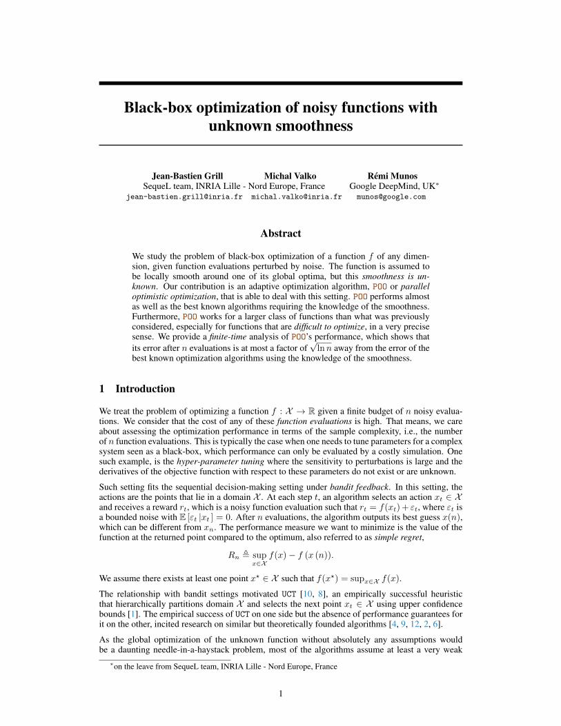
Figure 1: Difficult function f : x → s (log2 |x− 0.5|) · (√|x− 0.5| − (x− 0.5)
2) −
√|x− 0.5|
where, s(x) = 1 if the fractional part of x, that is, x − bxc, is in [0, 0.5] and s(x) = 0, if it is in(0.5, 1). Left: Oscillation between two envelopes of different smoothness leading to a nonzero d fora standard partitioning. Right: Simple regret of HOO after 5000 evaluations for different values of ρ.
Another direction has been followed by Munos [11], where in the deterministic case (the functionevaluations are not perturbed by noise), their SOO algorithm performs almost as well as the bestknown algorithms without the knowledge of the function smoothness. SOO was later extended toStoSOO [15] for the stochastic case. However StoSOO only extends SOO for a limited case of easyinstances of functions for which there exists a semi-metric under which d = 0. Also, Bull [6]provided a similar simple regret bound for ATB for a class of functions, called zooming continuousfunctions, which is related to the class of functions for which there exists a semi-metric under whichthe near-optimality dimension is d = 0. But none of the prior work considers a more general classof functions where there is no semi-metric adapted to the standard partitioning for which d = 0.
To give an example of a difficult function, consider the function in Figure 1. It possesses a lowerand upper envelope around its global optimum that are equivalent to x2 and
√x; and therefore
have different smoothness. Thus, for a standard partitioning, there is no semi-metric of the form`(x, y) = ||x − y||α for which the near-optimality dimension is d = 0, as shown by Valko et al.[15]. Other examples of nonzero near-optimality dimension are the functions that for a standardpartitioning behave differently depending on the direction, for instance f : (x, y) 7→ 1− |x| − y2.
Using a bad value for the ρ parameter can have dramatic consequences on the simple regret. InFigure 1, we show the simple regret after 5000 function evaluations for different values of ρ. For thevalues of ρ that are too low, the algorithm does not explore enough and is stuck in a local maximumwhile for values of ρ too high the algorithm wastes evaluations by exploring too much.
In this paper, we provide a new algorithm, POO, parallel optimistic optimization, which competeswith the best algorithms that assume the knowledge of the function smoothness, for a larger classof functions than was previously done. Indeed, POO handles a panoply of functions, including hardinstances, i.e., such that d > 0, like the function illustrated above. We also recover the result ofStoSOO and ATB for functions with d = 0. In particular, we bound the POO’s simple regret as
E[Rn] ≤ O(((
ln2 n)/n)1/(2+d(ν?,ρ?))
).
This result should be compared to the simple regret of the best known algorithm that uses the knowl-edge of the metric under which the function is smooth, or equivalently (ν, ρ), which is of the order ofO((lnn/n)1/(2+d)). Thus POO’s performance is at most a factor of (lnn)1/(2+d) away from that ofthe best known optimization algorithms that require the knowledge of the function smoothness. In-terestingly, this factor decreases with the complexity measure d: the harder the function to optimize,the less important it is to know its precise smoothness.
2 Background and assumptions
2.1 Hierarchical optimistic optimization
POO optimizes functions without the knowledge of their smoothness using a subroutine, an anytimealgorithm optimizing functions using the knowledge of their smoothness. In this paper, we use amodified version of HOO [4] as such subroutine. Therefore, we embark with a quick review of HOO.
HOO follows an optimistic strategy close to UCT [10], but unlike UCT, it uses proper confidencebounds to provide theoretical guarantees. HOO refines a partition of the space based on a hierarchicalpartitioning, where at each step, a yet unexplored cell (a leaf of the corresponding tree) is selected,
3

and the function is evaluated at a point within this cell. The selected path (from the root to the leaf)is the one that maximizes the minimum value Uh,i(t) among all cells of each depth, where the valueUh,i(t) of any cell Ph,i is defined as
Uh,i(t) = µh,i(t) +
√2 ln(t)
Nh,i(t)+ νρh,
where t is the number of evaluations done so far, µh,i(t) is the empirical average of all evaluationsdone within Ph,i, and Nh,i(t) is the number of them. The second term in the definition of Uh,i(t) isa Chernoff-Hoeffding type confidence interval, measuring the estimation error induced by the noise.The third term, νρh with ρ ∈ (0, 1) is, by assumption, a bound on the difference f(x?) − f(x) forany x ∈ Ph,i?h , a cell containing x?. It is this bound, where HOO relies on the knowledge of thesmoothness, because the algorithm requires the values of ν and ρ. In the next sections, we clarifythe assumptions made by HOO vs. related algorithms and point out the differences with POO.
2.2 Assumptions made in prior work
Most of previous work relies on the knowledge of a semi-metric on X such that the function is eitherlocally smooth near to one of its maxima with respect to this metric [11, 15, 2] or require a stronger,weakly-Lipschitz assumption [4, 12, 2]. Furthermore, Kleinberg et al. [9] assume the full metric.Note, that the semi-metric does not require the triangular inequality to hold. For instance, considerthe semi-metric `(x, y) = ||x − y||α on Rp with || · || being the euclidean metric. When α < 1then this semi-metric does not satisfy the triangular inequality. However, it is a metric for α ≥ 1.Therefore, using only semi-metric allows us to consider a larger class of functions.
Prior work typically requires two assumptions. The first one is on semi-metric ` and the function.An example is the weakly-Lipschitz assumption needed by Bubeck et al. [4] which requires that
∀x, y ∈ X , f(x?)− f(y) ≤ f(x?)− f(x) + max f(x?)− f(x), ` (x, y).It is a weak version of a Lipschitz condition, restricting f in particular for the values close to f(x?).
More recent results [11, 15, 2] assume only a local smoothness around one of the function maxima,
x ∈ X f(x?)− f(x) ≤ `(x?, x).
The second common assumption links the hierarchical partitioning with the semi-metric. It requiresthe partitioning to be adapted to the (semi) metric. More precisely the well-shaped assumption statesthat there exist ρ < 1 and ν1 ≥ ν2 > 0, such that for any depth h ≥ 0 and index i = 1, . . . , Ih, thesubset Ph,i is contained by and contains two open balls of radius ν1ρ
h and ν2ρh respectively, where
the balls are w.r.t. the same semi-metric used in the definition of the function smoothness.
‘Local smoothness’ is weaker than ‘weakly Lipschitz’ and therefore preferable. Algorithms requir-ing the local-smoothness assumption always sample a cell Ph,i in a special representative point and,in the stochastic case, collect several function evaluations from the same point before splitting thecell. This is not the case of HOO, which allows to sample any point inside the selected cell and toexpand each cell after one sample. This additional flexibility comes at the price of requiring thestronger weakly-Lipschitzness assumption. Nevertheless, although HOO does not wait before ex-panding a cell, it does something similar by selecting a path from the root to this leaf that maximizesthe minimum of the U -value over the cells of the path, as mentioned in Section 2.1. The fact thatHOO follows an optimistic strategy even after reaching the cell that possesses the minimal U -valuealong the path is not used in the analysis of the HOO algorithm.
Furthermore, a reason for better dependency on the smoothness in other algorithms, e.g., HCT [2],is not only algorithmic: HCT needs to assume a slightly stronger condition on the cell, i.e., that thesingle center of the two balls (one that covers and the other one that contains the cell) is actually thesame point that HCT uses for sampling. This is stronger than just assuming that there simply existsuch centers of the two balls, which are not necessarily the same points where we sample (which isthe HOO assumption). Therefore, this is in contrast with HOO that samples any point from the cell. Infact, it is straightforward to modify HOO to only sample at a representative point in each cell and onlyrequire the local-smoothness assumption. In our analysis and the algorithm, we use this modifiedversion of HOO, thereby profiting from this weaker assumption.
4

Prior work [9, 4, 11, 2, 12] often defined some ‘dimension’ d of the near-optimal space of f measuredaccording to the (semi-) metric `. For example, the so-called near-optimality dimension [4] measuresthe size of the near-optimal space Xε = x ∈ X : f(x) > f(x?)− ε in terms of packing numbers:For any c > 0, ε0 > 0, the (c, ε0)-near-optimality dimension d of f with respect to ` is defined as
infd ∈ [0,∞) : ∃C s.t. ∀ε ≤ ε0, N (Xcε, `, ε) ≤ Cε−d
, (1)
where for any subset A ⊆ X , the packing number N (A, `, ε) is the maximum number of disjointballs of radius ε contained in A.
2.3 Our assumption
Contrary to the previous approaches, we need only a single assumption. We do not introduce any(semi)-metric and instead directly relate f to the hierarchical partitioning P , defined in Section 1.Let K be the maximum number of children cells (Ph+1,jk)1≤k≤K per cell Ph,i. We remind thereader that given a global maximum x? of f , i?h denotes the index of the unique cell of depth hcontaining x?, i.e., such that x? ∈ Ph,i?h . With this notation we can state our sole assumption onboth the partitioning (Ph,i) and the function f .Assumption 1. There exists ν > 0 and ρ ∈ (0, 1) such that
∀h ≥ 0,∀x ∈ Ph,i?h , f(x) ≥ f (x?)− νρh.
The values (ν, ρ) defines a lower bound on the possible drop of f near the optimum x? accordingto the partitioning. The choice of the exponential rate νρh is made to cover a very large class offunctions, as well as to relate to results from prior work. In particular, for a standard partitioning onRp and any α, β > 0, any function f such that f(x) ∼x→x? β||x− x?||α fits this assumption. Thisis also the case for more complicated functions such as the one illustrated in Figure 1. An exampleof a function and a partitioning that does not satisfy this assumption is the function f : x 7→ 1/ lnxand a standard partitioning of [0, 1) because the function decreases too fast around x? = 0. Asobserved by Valko [15], this assumption can be weaken to hold only for values of f that are η-closeto f(x?) up to an η-dependent constant in the simple regret.
Let us note that the set of assumptions made by prior work (Section 2.2) can be reformulated usingsolely Assumption 1. For example, for any f(x) ∼x→x? β||x− x?||α, one could consider the semi-metric `(x, y) = β||x − y||α for which the corresponding near-optimality dimension defined byEquation 1 for a standard partitioning is d = 0. Yet we argue that our setting provides a more naturalway to describe the complexity of the optimization problem for a given hierarchical partitioning.
Indeed, existing algorithms, that use a hierarchical partitioning of X , like HOO, do not use the fullmetric information but instead only use the values ν and ρ, paired up with the partitioning. Hence,the precise value of the metric does not impact the algorithms’ decisions, neither their performance.What really matters, is how the hierarchical partitioning of X fits f . Indeed, this fit is what wemeasure. To reinforce this argument, notice again that any function can be trivially optimized givena perfectly adapted partitioning, for instance the one that associates x? to one child of the root.
Also, the previous analyses tried to provide performance guaranties based only on the metric and f .However, since the metric is assumed to be such that the cells of the partitioning are well shaped,the large diversity of possible metrics vanishes. Choosing such metric then comes down to choosingonly ν, ρ, and a hierarchical decomposition of X . Another way of seeing this is to remark thatprevious works make an assumption on both the function and the metric, and an other on both themetric and the partitioning. We underline that the metric is actually there just to create a link betweenthe function and the partitioning. By discarding the metric, we merge the two assumptions into asingle one and convert a topological problem into a combinatorial one, leading to easier analysis.
To proceed, we define a new near-optimality dimension. For any ν > 0 and ρ ∈ (0, 1), the near-optimality dimension d(ν, ρ) of f with respect to the partitioning P is defined as follows.Definition 1. Near-optimality dimension of f is
d(ρ) , infd′ ∈ R+ : ∃C > 0, ∀h ≥ 0, Nh(2νρh) ≤ Cρ−d′h
,
where Nh(ε) is the number of cells Ph,i of depth h such that supx∈Ph,if(x) ≥ f(x?)− ε.
5

The hierarchical decomposition of the space X is the only prior information available to the algo-rithm. The (new) near-optimality dimension is a measure of how well is this partitioning adaptedto f . More precisely, it is a measure of the size of the near-optimal set, i.e., the cells which are suchthat supx∈Ph,i
f(x) ≥ f(x?)− ε. Intuitively, this corresponds to the set of cells that any algorithmwould have to sample in order to discover the optimum.
As an example, any f such that f(x) ∼x→x? ||x− x?||α, for any α > 0, has a zero near-optimalitydimension with respect to the standard partitioning and an appropriate choice of ρ. As discussedby Valko et al. [15], any function such that the upper and lower envelopes of f near its maximum areof the same order has a near-optimality dimension of zero for a standard partitioning of [0, 1]. Anexample of a function with d > 0 for the standard partitioning is in Figure 1. Functions that behavedifferently in different dimensions have also d > 0 for the standard partitioning. Nonetheless, for asome handcrafted partitioning, it is possible to have d = 0 even for those troublesome functions.
Under our new assumption and our new definition of near-optimality dimension, one can prove thesame regret bound for HOO as Bubeck et al. [4] and the same can be done for other related algorithms.
3 The POO algorithm
3.1 Description of POO
The POO algorithm uses, as a subroutine, an optimizing algorithm that requires the knowledge ofthe function smoothness. We use HOO [4] as the base algorithm, but other algorithms, such asHCT [2], could be used as well. POO, with pseudocode in Algorithm 1, runs several HOO instancesin parallel, hence the name parallel optimistic optimization. The number of base HOO instances andother parameters are adapted to the budget of evaluations and are automatically decided on the fly.
Algorithm 1 POOParameters: K, P = Ph,i
Optional parameters: ρmax, νmax
Initialization:Dmax ← lnK/ ln (1/ρmax)n← 0 number of evaluation performedN ← 1 number of HOO instancesS ← (νmax, ρmax) set of HOO instances
while computational budget is available dowhile N ≤ 1
2Dmax ln (n/(lnn)) dofor i← 1, . . . , N do start new HOOss←
(νmax, ρmax
2N/(2i+1))
S ← S ∪ sPerform n
N function evaluation with HOO(s)Update the average reward µ[s] of HOO(s)
end forn← 2nN ← 2N
end whileensure there is enough HOOsfor s ∈ S do
Perform a function evaluation with HOO(s)Update the average reward µ[s] of HOO(s)
end forn← n+N
end whiles? ← argmaxs∈S µ[s]Output: A random point evaluated by HOO(s?)
Each instance of HOO requires two realnumbers ν and ρ. Running HOOparametrized with (ρ, ν) that are far fromthe optimal one (ν?, ρ?)
3 would cause HOOto underperform. Surprisingly, our analy-sis of this suboptimality gap reveals that itdoes not decrease too fast as we stray awayfrom (ν?, ρ?). This motivates the follow-ing observation. If we simultaneously runa slew of HOOs with different (ν, ρ)s, oneof them is going to perform decently well.
In fact, we show that to achieve good per-formance, we only require (lnn) HOO in-stances, where n is the current number offunction evaluations. Notice, that we donot require to know the total number ofrounds in advance which hints that we canhope for a naturally anytime algorithm.
The strategy of POO is quite simple: Itconsists of running N instances of HOO inparallel, that are all launched with differ-ent (ν, ρ)s. At the end of the whole pro-cess, POO selects the instance s? whichperformed the best and returns one of thepoints selected by this instance, chosenuniformly at random. Note that just us-ing a doubling trick in HOO with increasingvalues of ρ and ν is not enough to guaran-tee a good performance. Indeed, it is important to keep track of all HOO instances. Otherwise, theregret rate would suffer way too much from using the value of ρ that is too far from the optimal one.
3the parameters (ν, ρ) satisfying Assumption 1 for which d(ν, ρ) is the smallest
6

For clarity, the pseudo-code of Algorithm 1 takes ρmax and νmax as parameters but in Appendix Cwe show how to set ρmax and νmax automatically as functions of the number of evaluations, i.e.,ρmax (n), νmax (n). Furthermore, in Appendix D, we explain how to share information between theHOO instances which makes the empirical performance light-years better.
Since POO is anytime, the number of instances N(n) is time-dependent and does not need to beknown in advance. In fact, N(n) is increased alongside the execution of the algorithm. Moreprecisely, we want to ensure that
N(n) ≥ 12Dmax ln (n/ lnn) , where Dmax , (lnK)/ ln (1/ρmax) .
To keep the set of different (ν, ρ)s well distributed, the number of HOOs is not increased one by onebut instead is doubled when needed. Moreover, we also require that HOOs run in parallel, perform thesame number of function evaluations. Consequently, when we start running new instances, we firstensure to make these instances on par with already existing ones in terms of number of evaluations.
Finally, as our analysis reveals, a good choice of parameters (ρi) is not a uniform gridon [0, 1]. Instead, as suggested by our analysis, we require that 1/ ln(1/ρi) is a uniform gridon [0, 1/(ln 1/ρmax)]. As a consequence, we add HOO instances in batches such that ρi = ρmax
N/i.
3.2 Upper bound on POO’s simple regret
POO does not require the knowledge of a (ν, ρ) verifying Assumption 1 and4 yet we prove that itachieves a performance close5 to the one obtained by HOO using the best parameters (ν?, ρ?). Thisresult solves the open question of Valko et al. [15], whether the stochastic optimization of f withunknown parameters (ν, ρ) when d > 0 for the standard partitioning is possible.
Theorem 1. Let Rn be the simple regret of POO at step n. For any (ν, ρ) verifying Assumption 1such that ν ≤ νmax and ρ ≤ ρmax there exists κ such that for all n
E[Rn] ≤ κ ·((
ln2 n)/n)1/(d(ν,ρ)+2)
.
Moreover, κ = α ·Dmax(νmax/ν?)Dmax , where α is a constant independent of ρmax and νmax.
We prove Theorem 1 in the Appendix A and B. Notice that Theorem 1 holds for any ν ≤ νmax
and ρ ≤ ρmax and in particular for the parameters (ν?, ρ?) for which d(ν, ρ) is minimal as long asν? ≤ νmax and ρ? ≤ ρmax. In Appendix C, we show how to make ρmax and νmax optional.
To give some intuition on Dmax, it is easy to prove that it is the attainable upper bound on the near-optimality dimension of functions verifying Assumption 1 with ρ ≤ ρmax. Moreover, any functionof [0, 1]p, Lipschitz for the Euclidean metric, has (lnK)/ ln (1/ρ) = p for a standard partitioning.
The POO’s performance should be compared to the simple regret of HOO run with the best parame-ters ν? and ρ?, which is of order
O(
((lnn) /n)1/(d(ν?,ρ?)+2)
).
Thus POO’s performance is only a factor of O((lnn)1/(d(ν?,ρ?)+2)
) away from the optimally fittedHOO. Furthermore, our simple regret bound for POO is slightly better than the known simple regretbound for StoSOO [15] in the case when d(ν, ρ) = 0 for the same partitioning, i.e., E[Rn] =O (lnn/
√n) . With our algorithm and analysis, we generalize this bound for any value of d ≥ 0.
Note that we only give a simple regret bound for POO whereas HOO ensures a bound on both the cu-mulative and simple regret.6 Notice that since POO runs several HOOs with non-optimal values of the(ν, ρ) parameters, this algorithm explores much more than optimally fitted HOO, which dramaticallyimpacts the cumulative regret. As a consequence, our result applies to the simple regret only.
4note that several possible values of those parameters are possible for the same function5up to a logarithmic term
√lnn in the simple regret
6in fact, the bound on the simple regret is a direct consequence of the bound on the cumulative regret [3]
7

100 200 300 400 500
number of evaluations
0.06
0.08
0.10
0.12
0.14
0.16
0.18
sim
ple
regr
et
HOO, ρ = 0.0
HOO, ρ = 0.3
HOO, ρ = 0.66
HOO, ρ = 0.9
POO
4 5 6 7 8
number of evaluation (log-scaled)
−4.0
−3.5
−3.0
−2.5
−2.0
sim
ple
regr
et(lo
g-sc
aled
)
HOO, ρ = 0.0
HOO, ρ = 0.3
HOO, ρ = 0.66
HOO, ρ = 0.9
POO
Figure 2: Simple regret of POO and HOO run for different values of ρ.
4 Experiments
We ran experiments on the function plotted in Figure 1 for HOO algorithms with different values of ρand the POO7 algorithm for ρmax = 0.9. This function, as described in Section 1, has an upper andlower envelope that are not of the same order and therefore has d > 0 for a standard partitioning.
In Figure 2, we show the simple regret of the algorithms as function of the number of evaluations.In the figure on the left, we plot the simple regret after 500 evaluations. In the right one, we plotthe simple regret after 5000 evaluations in the log-log scale, in order to see the trend better. TheHOO algorithms return a random point chosen uniformly among those evaluated. POO does the samefor the best empirical instance of HOO. We compare the algorithms according to the expected simpleregret, which is the difference between the optimum and the expected value of function value at thepoint they return. We compute it as the average of the value of the function for all evaluated points.While we did not investigate possibly different heuristics, we believe that returning the deepestevaluated point would give a better empirical performance.
As expected, the HOO algorithms using values of ρ that are too low, do not explore enough andbecome quickly stuck in a local optimum. This is the case for both UCT (HOO run for ρ = 0) andHOO run for ρ = 0.3. The HOO algorithm using ρ that is too high waste their budget on exploringtoo much. This way, we empirically confirmed that the performance of the HOO algorithm is greatlyimpacted by the choice of this ρ parameter for the function we considered. In particular, at T = 500,the empirical simple regret of HOO with ρ = 0.66 was a half of the simple regret of UCT.
In our experiments, HOO with ρ = 0.66 performed the best which is a bit lower than what the theorywould suggest, since ρ? = 1/
√2 ≈ 0.7. The performance of HOO using this parameter is almost
matched by POO. This is surprising, considering the fact the POO was simultaneously running 100different HOOs. It shows that carefully sharing information between the instances of HOO, as describedand justified in Appendix D, has a major impact on empirical performance. Indeed, among the 100HOO instances, only two (on average) actually needed a fresh function evaluation, the 98 could reusethe ones performed by another HOO instance.
5 Conclusion
We introduced POO for global optimization of stochastic functions with unknown smoothness andshowed that it competes with the best known optimization algorithms that know this smoothness.This results extends the previous work of Valko et al. [15], which is only able to deal with a near-optimality dimension d = 0. POO is provably able to deal with a trove of functions for which d ≥ 0for a standard partitioning. Furthermore, we gave a new insight on several assumptions required byprior work and provided a more natural measure of the complexity of optimizing a function given ahierarchical partitioning of the space, without relying on any (semi-)metric.
Acknowledgements The research presented in this paper was supported by French Ministryof Higher Education and Research, Nord-Pas-de-Calais Regional Council, a doctoral grant ofEcole Normale Superieure in Paris, Inria and Carnegie Mellon University associated-team projectEduBand, and French National Research Agency project ExTra-Learn (n.ANR-14-CE24-0010-01).
7code available at https://sequel.lille.inria.fr/Software/POO
8

References[1] Peter Auer, Nicolo Cesa-Bianchi, and Paul Fischer. Finite-time analysis of the multiarmed
bandit problem. Machine Learning, 47(2-3):235–256, 2002.[2] Mohammad Gheshlaghi Azar, Alessandro Lazaric, and Emma Brunskill. Online stochastic op-
timization under correlated bandit feedback. In International Conference on Machine Learn-ing, 2014.
[3] Sebastien Bubeck, Remi Munos, and Gilles Stoltz. Pure exploration in finitely-armed andcontinuous-armed bandits. Theoretical Computer Science, 412(19):1832–1852, 2011.
[4] Sebastien Bubeck, Remi Munos, Gilles Stoltz, and Csaba Szepesvari. X -armed bandits. Jour-nal of Machine Learning Research, 12:1587–1627, 2011.
[5] Sebastien Bubeck, Gilles Stoltz, and Jia Yuan Yu. Lipschitz Bandits without the LipschitzConstant. In Algorithmic Learning Theory, 2011.
[6] Adam D. Bull. Adaptive-treed bandits. Bernoulli, 21(4):2289–2307, 2015.[7] Richard Combes and Alexandre Proutiere. Unimodal bandits: Regret lower bounds and opti-
mal algorithms. In International Conference on Machine Learning, 2014.[8] Pierre-Arnaud Coquelin and Remi Munos. Bandit algorithms for tree search. In Uncertainty
in Artificial Intelligence, 2007.[9] Robert Kleinberg, Aleksandrs Slivkins, and Eli Upfal. Multi-armed bandit problems in metric
spaces. In Symposium on Theory Of Computing, 2008.[10] Levente Kocsis and Csaba Szepesvari. Bandit-based Monte-Carlo planning. In European
Conference on Machine Learning, 2006.[11] Remi Munos. Optimistic optimization of deterministic functions without the knowledge of its
smoothness. In Neural Information Processing Systems, 2011.[12] Remi Munos. From bandits to Monte-Carlo tree search: The optimistic principle applied to
optimization and planning. Foundations and Trends in Machine Learning, 7(1):1–130, 2014.[13] Philippe Preux, Remi Munos, and Michal Valko. Bandits attack function optimization. In
Congress on Evolutionary Computation, 2014.[14] Aleksandrs Slivkins. Multi-armed bandits on implicit metric spaces. In Neural Information
Processing Systems, 2011.[15] Michal Valko, Alexandra Carpentier, and Remi Munos. Stochastic simultaneous optimistic
optimization. In International Conference on Machine Learning, 2013.
9

A Proof sketch of Theorem 1
In this part we give the roadmap of the proof. The full proof is in Appendix B.
First step For any choice of ρ? verifying Assumption 1 and any suboptimal ρ such that
0 < ρ? ≤ ρ < 1,
we bound the difference of near-optimality dimension,
d (ρ)− d (ρ?) ≤ lnK
(1
ln (1/ρ)− 1
ln (1/ρ?)
)and deduce that
mini:ρi≥ρ?
[d(ρi)− d(ρ?)] ≤Dmax
N·
Second step By simultaneously running a large number of HOO instances, we ensure that for allρ? ≤ ρmax, one of them uses a ρ close to ρ? and therefore suffers a low regret. On the other hand,simultaneously running a large number of HOOs has a cost, as more evaluations need to be done ateach step, one for each HOO. We optimize this tradeoff to deduce the following good choice of δ,which is the maximum distance |d (ρi)− d(ρj)|, where i and j are two consecutive HOOs.
δ = O (ln (t/ ln t)) .
Third step Using the result of the second step, we can compute the simple regret Rρn of the HOOinstance running with the parameter ρ > ρ?, which is the closest to ρ?. Note that, as POO is running,the instance it choose may change over time and so ρ depends on n.
We prove that there exists a constant α > 0 such that for all n, νmax > 0, and ρmax < 1,
Rρn ≤ α ·Dmax(νmax/ν?)Dmax
((ln2 n
)/n)1/(d(ρ)+2)
.
Fourth step At the end of the algorithm, we empirically determine which HOO performed the best.However, this best empirical instance may not be the instance running with ρ closest to the optimalunknown ρ?. Nonetheless, we prove that this error is small enough such that it only impacts thesimple regret by a constant factor.
B Full proof of Theorem 1
B.1 First step
We show that for any choice of ρ? verifying Assumption 1 and any ρ such that 0 < ρ? ≤ ρ < 1,
d (ρ)− d (ρ?) ≤ lnK
(1
ln (1/ρ)− 1
ln (1/ρ?)
)·
We start by defining Ih(ε) as the set of cells of depth h which are ε-near-optimal,
Ih (ε) ,
i : sup
x∈Ph,i
f(x) ≥ f(x?)− ε·
Nh(ε), defined in Section 1, is then equal to the cardinality of Ih(ε). Notice that if a cell (h, i) isε-near-optimal then all of its antecedents are also ε-near-optimal. Therefore, for any ε and h′ > h,the cells in Ih′(ε) are descendants of the cells in Ih(ε).
Since the number of descendants at depth h′ of a cell at depth h′ > h is bounded by Kh′−h webound the cardinality Nh(ε) of Ih′(ε),
∀ε,∀h′ > h, Nh′(ε) ≤ Kh′−hNh(ε).
10
By definition of the near-optimality dimension, we know that for any ν > 0 and ρ? ∈ (0, 1), thereexists C such that for all h,
Nh(2νρh
)≤ Cρ−d(ρ)h.
We define C(ν, ρ) as the smallest C verifying the above condition.
For any 0 < ν? < ν, 0 < ρ? < ρ < 1 and any integer h ≥ hmin , ln(ν/ν?)/ ln(1/ρ) let us defineh? as the greatest integer such that νρh < ν?ρ
h?? . From this definition, we get νρh ≥ ν?ρh?+1
? fromwhich we deduce that
h? ≥ h ·ln ρ
ln ρ?+
ln ν − ln ν?ln ρ?
− 1,
and then
h− h? ≤ h? ln ρ?
(1
ln ρ− 1
ln ρ?
)+
ln ρ? + ln ν? − ln ν
ln ρ·
Since Nh(ε) is not increasing in ε, νρh < ν?ρh?? implies
Nh(2νρh) ≤ Nh(2ν?ρh?? ).
We now put everything together to obtain
Nh(2νρh) ≤ Nh(2ν?ρh?? )
≤ Kh−h?Nh?(2ν?ρh?? )
≤ K(ln ρ?+ln ν?−ln ν)/ ln ρ+h? ln ρ?(1/ ln ρ−1/ ln ρ?)C(ν?, ρ?)ρ−d(ρ?)h??
≤ C(ν?, ρ?)K(ln ρ?+ln ν?−ln ν)/ ln ρρ
−h?[d(ρ?)+lnK(1/ ln(1/ρ)−1/ ln(1/ρ?))]? .
From νρh < ν?ρh?? and ν? < ν we get ρ−h > ρ−h?
? and therefore
Nh(2νρh) ≤ C(ν?, ρ?)K(ln ρ?+ln ν?−ln ν)/ ln ρρ−h[d(ρ?)+lnK(1/ ln(1/ρ)−1/ ln(1/ρ?))].
We just proved that there exists C such that for all h > 0
Nh(2νρh) ≤ Cρ−h[d(ρ?)+lnK(1/ ln(1/ρ)−1/ ln(1/ρ?))].
By taking
C , max(C(ν?, ρ?)K
(ln ρ?+ln ν?−ln ν)/ ln ρ,Khmin
),
we deduce by the definition of the near-optimality dimension the following bound
d(ρ) ≤ d(ρ?) + lnK
(1
ln (1/ρ)− 1
ln (1/ρ?)
)·
We can now deduce that POO should use ρi parameters that satisfy
1
ln (1/ρi),
i
N
1
ln (1/ρmax),
where N is the total number of HOO instances run and i ∈ 1, . . . , N.We now define ρ as the closest ρi to ρ? used by an existing HOO instance, such that ρi > ρ?.
ρ , arg minρi≥ρ?
[d (ρi)− d (ρ?)] .
Since we assumed that ρ? < ρmax, we know that
d(ρ)− d(ρ?) ≤Dmax
N, with Dmax , (lnK)/ ln (1/ρmax) .
11

B.2 Second step
Let us now compute the optimal number of N instances to run in parallel. We bound the logarithmof the simple regret Rν,ρt of a single HOO instance using parameters ν and ρ after this particularinstance performed t function evaluations. In particular, we bound the simple regret by a linearapproximation for ρ ∼ ρ?. In the following, β is a numerical constant coming from the analysis ofHOO [4]. For all t > 0, we have
lnRν,ρt ≤ lnβ +lnC(ν, ρ)
2 + d(ρ)− ln (t/ ln t)
2 + d(ρ)
= lnβ +lnC(ν, ρ)
2 + d(ρ)− ln (t/ ln t)
2 + d(ρ?)· 1
1 + (d (ρ)− d (ρ?)) / (2 + d (ρ?))
≤ lnβ +lnC(ν, ρ)
2 + d(ρ)− ln (t/ ln t)
2 + d(ρ?)·(
1− d(ρ)− d(ρ?)
2 + d(ρ?)
)·
After n function evaluations by POO, each instance performed at least t = bn/Nc function eval-uations. We can now bound the simple regret RPOO,ν,ρ
n of the HOO instance using ν and ρ after nevaluations performed by all the instances
lnRPOO,ν,ρn ≤ lnβ +
lnC(ν, ρ)
2 + d(ρ)+ ln
(lnbn/Ncbn/Nc
)(1
2 + d(ρ?)− Dmax/N
(2 + d(ρ?))2
)· (2)
Optimizing this upper bound for N leads to the following choice of N ,
N ∼ 12Dmax ln (n/ lnn) .
Therefore, in POO we choose to ensure N ≥ 12Dmax ln (n/ lnn).
If the time horizon was known in advance,N could be any integer. Nevertheless, since the algorithmis anytime, all the previous HOO instances have to be kept and new instances need to be added inbetween. Therefore, we restrict N to be of the form 2i, for i ∈ N.
As a consequence of this choice, N can be at most 2 times its lower bound and therefore12Dmax ln (n/ lnn) ≤ N ≤ Dmax ln (n/ lnn) .
B.3 Third step
Using our choice of N , we can bound the simple regret of the HOO instance using ρ. We proceed byseparately bounding each of the terms in Equation 2.
lnC(ν, ρ)
2 + d(ρ)≤ 1
2 + d(ρ?)lnC(ν, ρ)
≤ 1
2 + d(ρ?)ln max
(C(ν?, ρ?)K
(ln ρ?+ln ν?−ln ν)/ ln ρ,Khmin
)≤ 1
2 + d(ρ?)max
(lnC(ν?ρ?)+lnK
(ln 1/ρ?ln 1/ρ
+ln (ν/ν?)
ln 1/ρ
), ln[K ln(ν/ν?)/ ln(1/ρ)
])≤ 1
2 + d(ρ?)max
(lnC(ν?ρ?)+max
(lnK ln ρ?Dmax
N, 2
)+
lnK ln νmax
ν?
ln 1/ρ,Dmax ln
ν
ν?
)≤ γ +
Dmax
2 + d(ρ?)ln (νmax/ν?)
In the last expression, γ is a quantity independent of νmax, ρmax, and N .
We now use N ≤ Dmax ln (n/ lnn) to get
ln
(lnbn/Ncbn/Nc
)≤ ln (Dmax lnn ln (n/ lnn) /n) .
12

To bound the last term, we use 12Dmax ln (n/ lnn) ≤ N to get
− ln
(lnbn/Ncbn/Nc
)Dmax/N
(2 + d(ρ?))2≤ ln
(1
Dmax· n
lnn· 1
ln (n/ lnn)
)1
2 ln (n/ lnn)≤ 2.
We can finally bound the simple regretRPOO,ρn of the HOO instance using ρ after n function evaluations
overall. Combining the results above, we know that for all n, νmax, and ρmax,
RPOO,ρn ≤ β exp(γ + 2)
(Dmax (νmax/ν?)
Dmax (lnn) ln (n/ lnn) /n)1/(2+d(ρ))
.
We bound ln (n/ lnn) by lnn to get the following bound. There exists α that is independent of ρmaxand νmax, such that
RPOO,ρn ≤ α ·Dmax(νmax/ν?)
Dmax((
ln2 n)/n)1/(d(ρ)+2)
.
B.4 Fourth step
Let (Xi,j)i≤n,j≤N be a family of points in X evaluated by POO. We denote f(Xi,j) the noisy eval-uation at Xi,j and f(Xi,j) = E[f(Xi,j)]. We also define:
µj ,1
n
n∑i=1
f(Xi,j) µj ,1
n
n∑i=1
f(Xi,j)
j , arg max1≤j≤N
µj j , arg max1≤j≤N
µj
By Hoeffding-Azuma inequality for martingale differences, for any ∆ > 0,
P
[n∑i=1
f(Xi,j)− f(Xi,j) > n∆
]≤ exp
(−2(n∆)2
n
)·
ThereforeP[µj − µj > ∆] ≤ exp
(−2n∆2
).
As we have
∀x ≥ 0, x · exp(−2nx2
)≤ e−2
2√n
,
we can now integrate exp(−2n∆2
)over ∆ ∈ [0, 1] to get
E[µj − µj ] ≤e−2
2√n·
Now consider
E[µj − µj
]= E [µj − µj ] + E
[µj − µj
]+ E
[µj − µj
].
Notice that the first and last term are both bounded by e−2/ (2√n) and the middle term is negative.
Finally, taking a union bound over the N variables µj we get
E[µj? − µj?
]≤ e−2N√
n·
As N = o (lnn), we conclude that this additional term is negligible with respect to
(lnn ln (n/ lnn) /n)1/(2+d(ρ?))
.
13

C Increasing sequence for ρmax and νmax
Besides the number K of children for each cell, POO needs two parameters, ρmax ∈ (0, 1) andνmax > 0. Theorem 1 states that POO run with those parameters performs almost as well as thebest instance of HOO run with ν ≤ νmax and ρ ≤ ρmax, i.e., corresponding to the near-optimalitydimension mind(ν, ρ), ν ≤ νmax, ρ ≤ ρmax.Therefore, the larger the values ρmax and νmax used by POO, the wider the set of HOO instances thatwe can compete with. Nevertheless, large values of ρmax and νmax impact the performance by amultiplicative constant of order Dmaxνmax
Dmax . This tradeoff between performance and size of ourcomparison class is unfortunate but unavoidable.
In practice, as we strive for an algorithm that does not require the knowledge of the smoothnesswe may increase the values of ρmax(n) and νmax(n) with the number of evaluations n, so thatthe class of functions covered by POO gets bigger with the numerical budget. Nevertheless, theincrease should be slow enough so that we do not compromise the performance. In particular, we willrequire that νmax(n)Dmax(n) does not increase too fast. In fact, any sequence ρmax(n) convergingto 1 and νmax(n) diverging to infinity impacts the simple regret by an additive term which is thesmallest time n such that ρ? < ρmax(n) and ν? < νmax(n), i.e., the first time the assumptions areverified. A slowly increasing sequence means a smaller impact on the simple regret rate but a higheradditive term (a constant independent of n). Any sensible choice of increasing sequence ρmax(n)and νmax(n), impacting the rate by only a subpolynomial factor, is a valid choice.
Algorithm 1 is described using constant ρmax and νmax for clarity, but its implementation is easilymodifiable to deal with increasing values of these two parameters while preserving the anytime prop-erty of the algorithm, as follows. At any time, all the HOO instances must use the same νmax parame-ter. On the other hand, considering ρmax, the value ofDmax has to be increased such that the alreadyrunning HOO instances stay relevant. One way to do that is to increaseDmax asDmax(N+1)/N andrun an additional HOO instance. An alternative solution is to perform, each time when needed, thefollowing increment ρmax ← √ρmax and runN additional HOO instances with parameters ρmax
2N/i,for i ∈ 1, . . . , N.
D Information sharing among parallel runs
Since we run several instances of HOO on the same partitioning of X , we may think of sharing thesamples among them, in order to decrease the estimation error. However, this needs to be done care-fully in order to avoid adding unwanted bias in the estimation of the U values in the HOO instances.Ideally, each HOO instance would reuse all function evaluations acquired by all other instances. Un-fortunately, this solution would not easily come with theoretical guaranties, as this would reduceartificially the confidence intervals at some cells and introduce search bias.
Instead, whenever a HOO instance requires a function evaluation, we perform a look-up to find outwhether another HOO instance has already evaluated f at this point. In affirmative, then instead ofevaluating the function at this point again, we simply reuse the sample. This way, HOO instancesare not given access to samples they never asked for. However, the empirical simple regrets ofHOOs becomes correlated with each other. This is not a problem because in B.4, we do not assumethe independence between empirical means of HOOs, only the independence of rewards within eachinstance—which still holds. Therefore with this modification, our theoretical guaranties continue toapply. Note that if all the instances share all their rewards, then they are all equivalent and there isno mistake possible. Then one can show, that the worst case is when no rewards are shared and theerror due to choosing the wrong instance actually decreases when the information is shared.
Finally, we want to stress that sharing information is extremely important in practice, as our ex-periments reveal. Since the number of HOO instances can be very large8 one could expect the per-formance of POO to be pitiful. However, as the vast majority of the function evaluations are inpractice shared, POO performs almost as well as HOO fitted with the best parameters. Summing up,although the performance bound on the simple regret with this modification is the same, empiricalperformance improves tremendously.
8even though it scales only as lnn with the number of evaluations n, it does not scale well with ρmax
14

E Zero-quality functions
For any ρ ∈ (0, 1), we construct a locally Lipschitz function with a rate ρ and a constant ν = 1 thatPOO can provably optimize and its quality, as defined by Definition 2, is zero. In order to properlydefine the quality, we use the uniform distribution on [0, 1] to sample from a node of the partitioning.Definition 2 (Slivkins [14]). The quality is the largest q ∈ (0, 1) such that for each subtree vcontaining the optimum, there exist nodes u and u′ such that P(u|v) and P(u′|v) are at least q and
|f(u)− f(u′)| ≥ 12 supx,y∈v
|f(x)− f(y)|.
We construct such function f on the interval [0, 1], its maximum being attained in x? = 0 withf(0) = 0. For any x 6= 0 we define f as follows. For any h ≥ 0 we define f on
(1
2h+1 ,1
2h
]as
∀x ∈(
1
2h+1, 1 + 1/(h+ 1)
2h+1
], f(x) = −ρh,
∀x ∈(
1 + 1/(h+ 1)
2h+1, 1
2h
], f(x) = −ρ
h
3·
We also consider the standard partitioning on [0, 1].
The optimal node of depth h corresponds to the interval[0, 2−h
]. By our definition of f ,
∀x ∈[0, 2−h
], f(0)− f(x) ≤ ρh
f(0)− f(
1 + 1/(h+ 1)
2h+1
)= ρh,
from which we conclude that f is locally Lipschitz with rate ρ and therefore can be optimized byPOO with provable finite-time guarantees (Theorem 1).
Now we prove that the quality of this function is zero. Using Definition 2, we can do it by showingthat there exists no such q ∈ (0, 1), for which there could be a node v along the optimal path with uand u′ verifying P(u|v) ≥ q (and same for u′) such that
supx∈u
f(x)− supx∈u′
f(x) ≥ supx∈v
f(0)− f(x)
2· (3)
Let q be a real number from (0, 1) and consider any h > 1/q. We pick v =[0, 2−h
].
P(
x ∈ v : f(x) ≤ −ρh
2
∣∣∣∣v) =
=1
2P(
x ∈[0,
1
2h+1
]: f(x) ≤ −ρ
h
2
∣∣∣∣v)+1
2P(
x ∈[
1
2h+1,
1
2h
]: f(x) ≤ −ρ
h
2
∣∣∣∣v)=
1
2P(
x ∈[0,
1
2h+1
]: f(x) ≤ −ρ
h
2
∣∣∣∣v)+1
2(h+ 1)
≤ 1
2
∞∑k=1
1
2k(h+ k + 1)+
1
2(h+ 1)
≤ 1
h+ 1< q
Notice that if u′ verifies (3), then u′ is included inx ∈ v : f(x) ≤ −ρh/2
. Combined with the
equation above, we have that
P(u|v) ≤ P(x ∈ v : f(x) ≤ −ρh/2
∣∣v) < q,
which is a contradiction. Since this holds for any q > 0, we deduce that the quality of f is zero.Yet f is Lipschitz with rate ρ ∈ (0, 1) and therefore f can be optimized by POO.
15