black carbon concentrations and diesel vehicle emission
TRANSCRIPT
1
Black Carbon Concentrations and Diesel Vehicle Emission Factors Derived from Coefficient of Haze Measurements in California: 1967-2003
Thomas W. Kirchstetter*, Jeffery Aguiar, Shaheen Tonse, T. Novakov Environmental Energy Technologies Division, Lawrence Berkeley National Laboratory, Berkeley CA, USA David Fairley Bay Area Air Quality Management District, Research and Modeling Division, San Francisco, CA, USA Abstract
We have derived ambient black carbon (BC) concentrations and estimated emission factors
for on-road diesel vehicles from archived Coefficient of Haze (COH) data that was
routinely collected beginning in 1967 at 11 locations in the San Francisco Bay Area. COH
values are a measure of the attenuation of light by particles collected on a white filter, and
available data indicate they are proportional to BC concentrations measured using the
conventional aethalometer. Monthly averaged BC concentrations are up to five times
greater in winter than summer, and, consequently, so is the population’s exposure to BC.
The seasonal cycle in BC concentrations is similar for all Bay Area sites, most likely due
to area-wide decreased pollutant dispersion during wintertime. A strong weekly cycle is
also evident, with weekend concentrations significantly lower than weekday
concentrations, consistent with decreased diesel traffic volume on weekends. The weekly
cycle suggests that, in the Bay Area, diesel vehicle emissions are the dominant source of
BC aerosol. Despite the continuous increase in diesel fuel consumption in California,
annual Bay Area average BC concentrations decreased by a factor of ~3 from the late
1960s to the early 2000s. Based on estimated annual BC concentrations, on-road diesel
fuel consumption, and recent measurements of on-road diesel vehicle BC emissions, diesel
BC emission factors decreased by an order of magnitude over the study period. Reductions
in the BC emission factor reflect improved engine technology, emission controls and
changes in diesel fuel composition. A new BC monitoring network is needed to continue
tracking ambient BC trends because the network of COH monitors has recently been
retired. _________________________________________________________________________
Keywords: coefficient of haze, black carbon, aethalometer, particulate matter, diesel vehicle, motor vehicle emissions, air quality, air pollution trends *Corresponding author email address: [email protected] and telephone:510.486.5319
2
1. Introduction
Black carbon (BC), a product of incomplete combustion of carbonaceous fuels, is
the main sunlight-absorbing component of atmospheric aerosols. The absorption of
sunlight by BC contributes to visibility degradation in polluted atmospheres [Horvath
1993] and to anthropogenic climate forcing [Jacobson 2001, Houghton et al. 2001]. BC
also poses a public health concern because it is present in particulate matter that is small
enough to deposit in the lungs, which causes asthma and other health problems [Pope and
Dockery 2006]. BC has been used as an indicator of exposure to diesel exhaust [e.g., Fruin
et al. 2004], which has been classified as a toxic air contaminant [CARB 1998] and a
suspected carcinogen [Cal EPA 2005].
Coal and diesel are the primary BC-producing fossil fuels. BC emissions are a
function of the combustion technology in addition to the amount and type of consumed
fuels. The combustion of BC in the United States and other industrialized countries has
changed markedly over time, as discussed in Novakov et al. [2003]. In the past, inefficient
coal combustion in the domestic and industrial sectors generated most of the anthropogenic
BC emissions. In the second half of the past century, however, petroleum-based fuels
replaced coal as the principal BC source in the United States and in Western Europe.
Presently, diesel engines in the transportation sector are the main sources of BC in
urban regions in the United States and elsewhere [Bond et al. 1994], and are thus
responsible for much of the environmental impacts of BC. It is clear that diesel fuel
consumption has increased in the U.S. over the past 30+ years [Cal BOE 2007]; and over
this period air pollution abatement policies have resulted in changes to diesel technology.
However, it is difficult to say how changing diesel technology has influenced ambient BC
concentrations because most measurements of BC concentration lack long-term and
regional coverage. Vehicle emission factors could be combined with fuel consumption data
to estimate the historical contribution of diesel vehicles to atmospheric BC, but published
emission factors differ by about a factor of ten [Cooke et al. 1999; Bond et al. 2004; Ito
and Penner 2005]. Therefore, significant uncertainty accompanies estimates of ambient
concentration trends based on published emission factors and fuel consumption data,
indicating the need for additional approaches, as suggested previously [Hansen et al.
2003].
3
In lieu of direct measurements of atmospheric BC concentrations, a retrospective
analysis of BC air pollution must rely on proxy data. Novakov and Hansen [2004]
estimated atmospheric BC concentrations from “black smoke” data in the U.K. Cass et al.
[1984] estimated BC concentrations from reflectance-based tape sampler measurements in
southern California. In this study, we used archived measurements of coefficient of haze
(COH) to estimate BC concentrations. COH was one of the earliest measures of particulate
matter air pollution adopted by regulatory agencies. COH levels were monitored
throughout California beginning in the late 1960s, but most COH monitors have now been
retired.
Like modern measurement of BC made with the aethalometer [Hansen et al. 1984],
COH measurement involved drawing a known volume of air through a white filter and
periodically measuring the light (from an incandescent bulb) transmitted through the
particle-laden filter to determine the aerosol optical density [Hemeon et al. 1953]. Whereas
BC is reported in units of mass concentration (µg m-3), the COH unit was defined as the
amount of aerosol that produced an optical density of 0.01. COH values express aerosol
concentrations in terms of COH per 1000 linear feet (305 m) of sampled air. As the optical
density of urban aerosols is largely due to light-absorbing black carbon, especially in the
visible and near-infrared wavelengths used to measure COH, COH values are highly
correlated with BC concentrations simultaneously measured using filter-based optical
methods [Cass et al. 1984; Allen et al. 1999].
The present analysis focuses on the San Francisco Bay Area of California. We use
COH measurements in this region to estimate how ambient BC concentrations have
changed during the past four decades. Our analysis first considers the relationship between
COH and BC and then the trends in BC concentrations over different time scales – weekly,
seasonal and long term. This provides information about predominant BC emission
sources, the population’s exposure to combustion-derived particulate matter, and the
impact of technology changes on ambient BC concentrations and emissions. Additionally,
we estimate the 30+ yr trend in on-road diesel vehicle BC emission factors.
2. Archived COH Data
COH levels recorded at approximately 100 sites throughout California are available
4
from the California Air Resources Board [CARB, 2006]. We analyzed archived COH data
from 11 sites in the San Francisco air basin over a 37-year period (1967 to 2003). These 11
sites, listed below, reported daily average COH values on most (65-96%) of the days in
this period. COH data from other sites in this air basin with limited coverage during this
period (4-34% of daily averages available) were excluded from the analysis.
The 11 included sites under the jurisdiction of the Bay Area Air Quality
Management District (BAAQMD) were Concord (Contra Costa county), Fremont
(Alameda county), Livermore (Alameda county), Napa (Napa county), Pittsburg (Contra
Costa county), Redwood City (San Mateo county), Richmond (Contra Costa county), San
Jose (Santa Clara county), San Rafael (Marin county), Santa Rosa (Sonoma county) and
Vallejo (Solano county). A map of the San Francisco air basin is available at the
BAAQMD’s website: http://www.baaqmd.gov/dst/jurisdiction.htm.
BAAQMD’s air pollution monitoring facilities are sited following EPA guidelines
and are intended to reflect major pollutant sources. They are located in urban areas where
pollutant concentrations are influenced by emissions from traffic on local streets. None of
the sites are immediately adjacent to a freeway, but many are within a mile or two,
including those at Livermore, Redwood City, San Jose and San Rafael. Both the Redwood
City and San Rafael sites have operated 30+ years and are within a few blocks of Highway
101.
The COH monitoring procedure was not fundamentally changed over the study
period (Yamaichi and Stevenson, personal communication, 2007). The most significant
change was a switch from manual to automated data acquisition. Thus, the COH trends
discussed below should not be due to changes in sampling methodology.
3. Results and Discussion
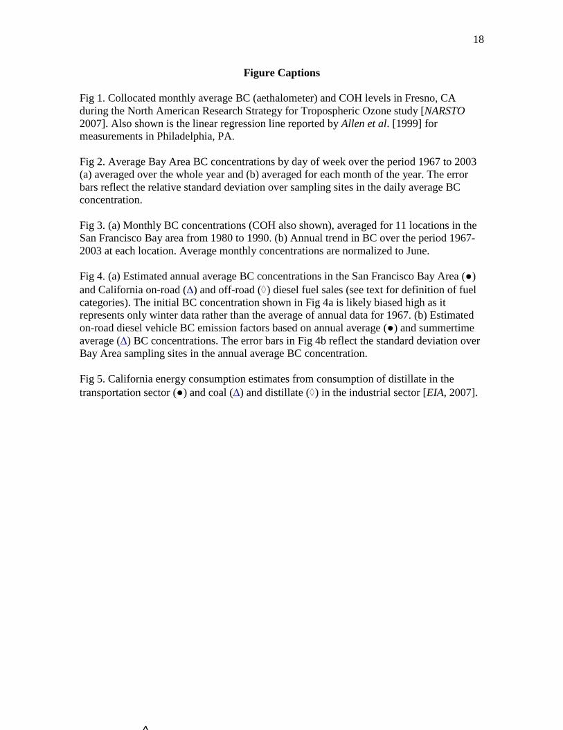
3.1 Relationship between COH and BC. The basis for using COH data to estimate
trends in BC stems from the similarity in the techniques used to measure both species, as
noted above. Allen et al. [1999] reported a strong linear relationship between COH levels
and aethalometer BC concentrations in Philadelphia during the summer of 1992: BC (µg
m-3) = 5.66•COH – 0.26 with R2 = 0.99 (where R2 is the linear correlation coefficient). As
shown in Fig 1, monthly average COH and BC measurements recorded in Fresno,
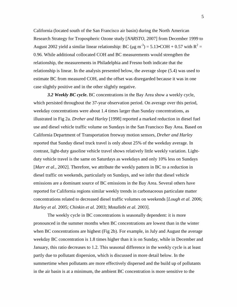
5
California (located south of the San Francisco air basin) during the North American
Research Strategy for Tropospheric Ozone study [NARSTO, 2007] from December 1999 to
August 2002 yield a similar linear relationship: BC (µg m-3) = 5.13•COH + 0.57 with R2 =
0.96. While additional collocated COH and BC measurements would strengthen the
relationship, the measurements in Philadelphia and Fresno both indicate that the
relationship is linear. In the analysis presented below, the average slope (5.4) was used to
estimate BC from measured COH, and the offset was disregarded because it was in one
case slightly positive and in the other slightly negative.
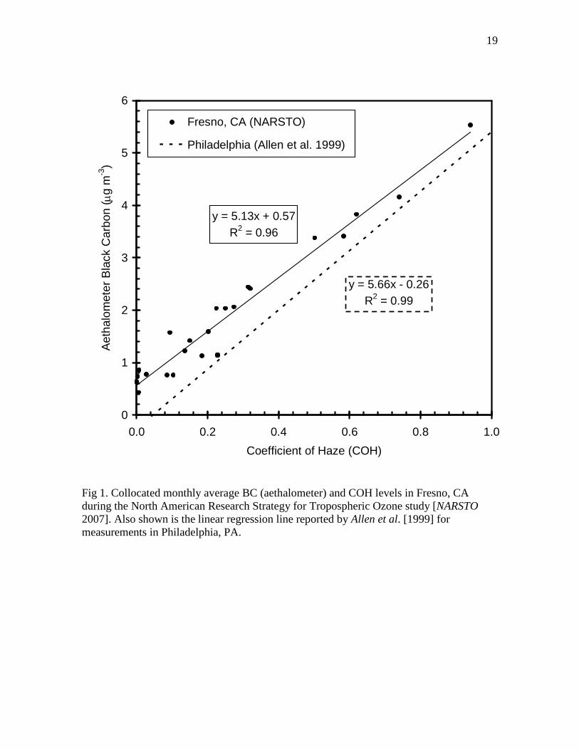
3.2 Weekly BC cycle. BC concentrations in the Bay Area show a weekly cycle,
which persisted throughout the 37-year observation period. On average over this period,
weekday concentrations were about 1.4 times larger than Sunday concentrations, as
illustrated in Fig 2a. Dreher and Harley [1998] reported a marked reduction in diesel fuel
use and diesel vehicle traffic volume on Sundays in the San Francisco Bay Area. Based on
California Department of Transportation freeway motion sensors, Dreher and Harley
reported that Sunday diesel truck travel is only about 25% of the weekday average. In
contrast, light-duty gasoline vehicle travel shows relatively little weekly variation. Light-
duty vehicle travel is the same on Saturdays as weekdays and only 10% less on Sundays
[Marr et al., 2002]. Therefore, we attribute the weekly pattern in BC to a reduction in
diesel traffic on weekends, particularly on Sundays, and we infer that diesel vehicle
emissions are a dominant source of BC emissions in the Bay Area. Several others have
reported for California regions similar weekly trends in carbonaceous particulate matter
concentrations related to decreased diesel traffic volumes on weekends [Lough et al. 2006;
Harley et al. 2005; Chinkin et al. 2003; Motallebi et al. 2003].
The weekly cycle in BC concentrations is seasonally dependent: it is more
pronounced in the summer months when BC concentrations are lowest than in the winter
when BC concentrations are highest (Fig 2b). For example, in July and August the average
weekday BC concentration is 1.8 times higher than it is on Sunday, while in December and
January, this ratio decreases to 1.2. This seasonal difference in the weekly cycle is at least
partly due to pollutant dispersion, which is discussed in more detail below. In the
summertime when pollutants are more effectively dispersed and the build up of pollutants
in the air basin is at a minimum, the ambient BC concentration is more sensitive to the
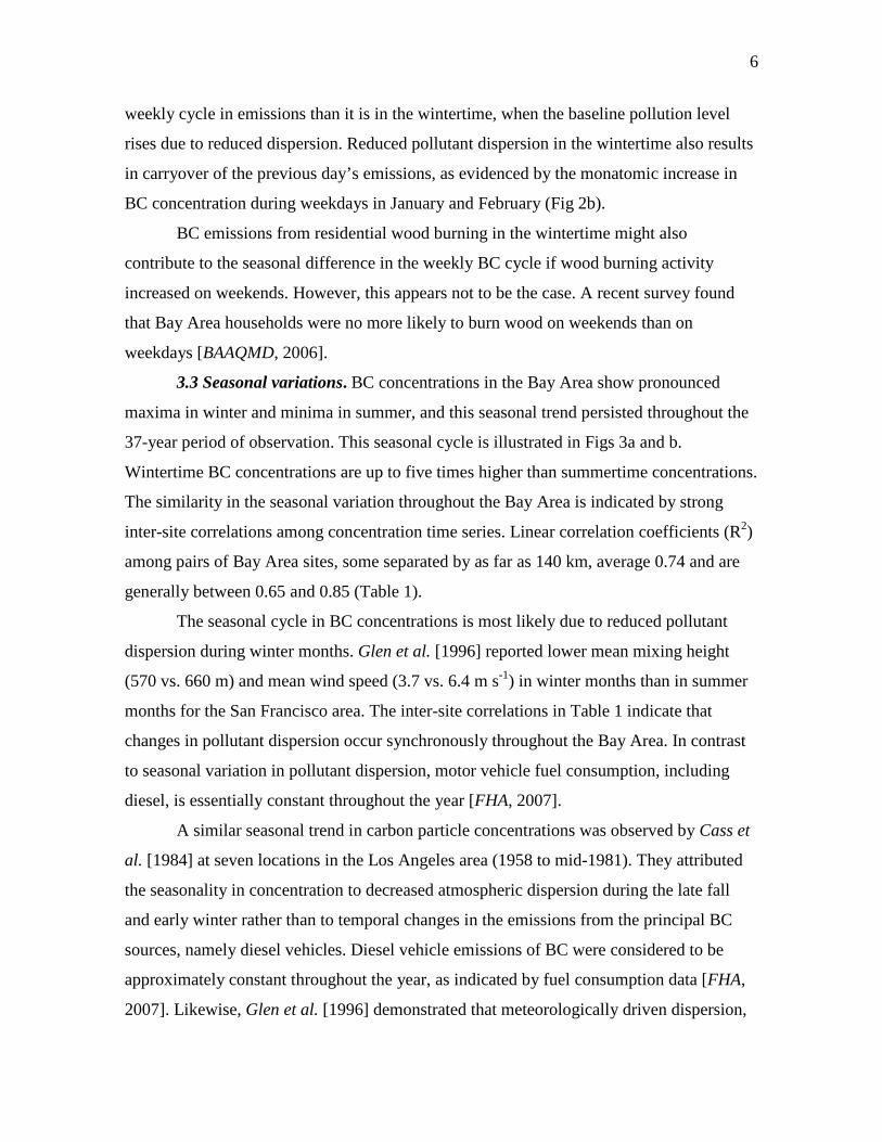
6
weekly cycle in emissions than it is in the wintertime, when the baseline pollution level
rises due to reduced dispersion. Reduced pollutant dispersion in the wintertime also results
in carryover of the previous day’s emissions, as evidenced by the monatomic increase in
BC concentration during weekdays in January and February (Fig 2b).
BC emissions from residential wood burning in the wintertime might also
contribute to the seasonal difference in the weekly BC cycle if wood burning activity
increased on weekends. However, this appears not to be the case. A recent survey found
that Bay Area households were no more likely to burn wood on weekends than on
weekdays [BAAQMD, 2006].
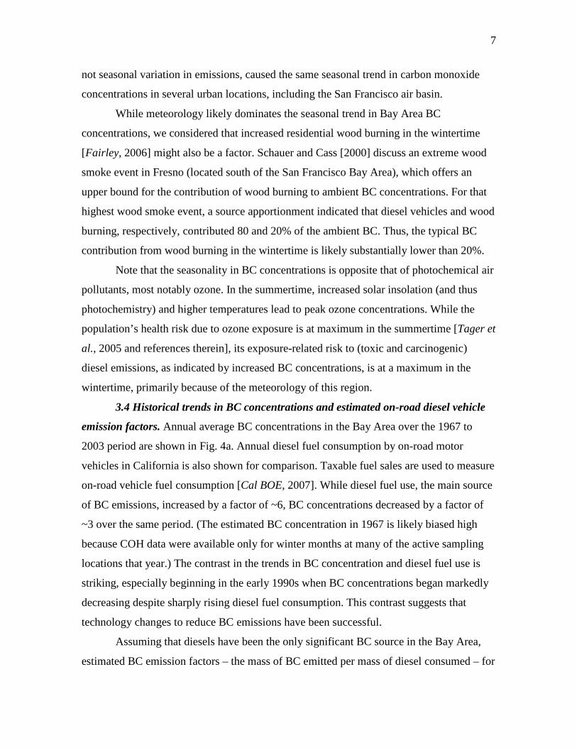
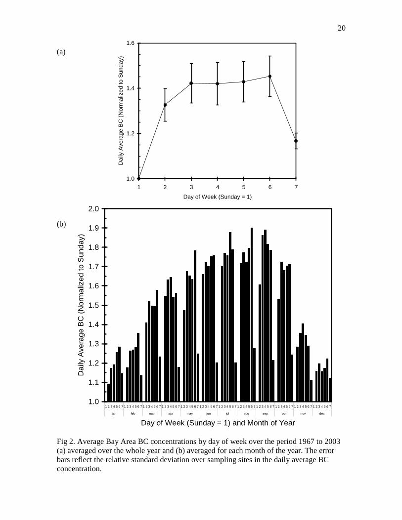
3.3 Seasonal variations. BC concentrations in the Bay Area show pronounced
maxima in winter and minima in summer, and this seasonal trend persisted throughout the
37-year period of observation. This seasonal cycle is illustrated in Figs 3a and b.
Wintertime BC concentrations are up to five times higher than summertime concentrations.
The similarity in the seasonal variation throughout the Bay Area is indicated by strong
inter-site correlations among concentration time series. Linear correlation coefficients (R2)
among pairs of Bay Area sites, some separated by as far as 140 km, average 0.74 and are
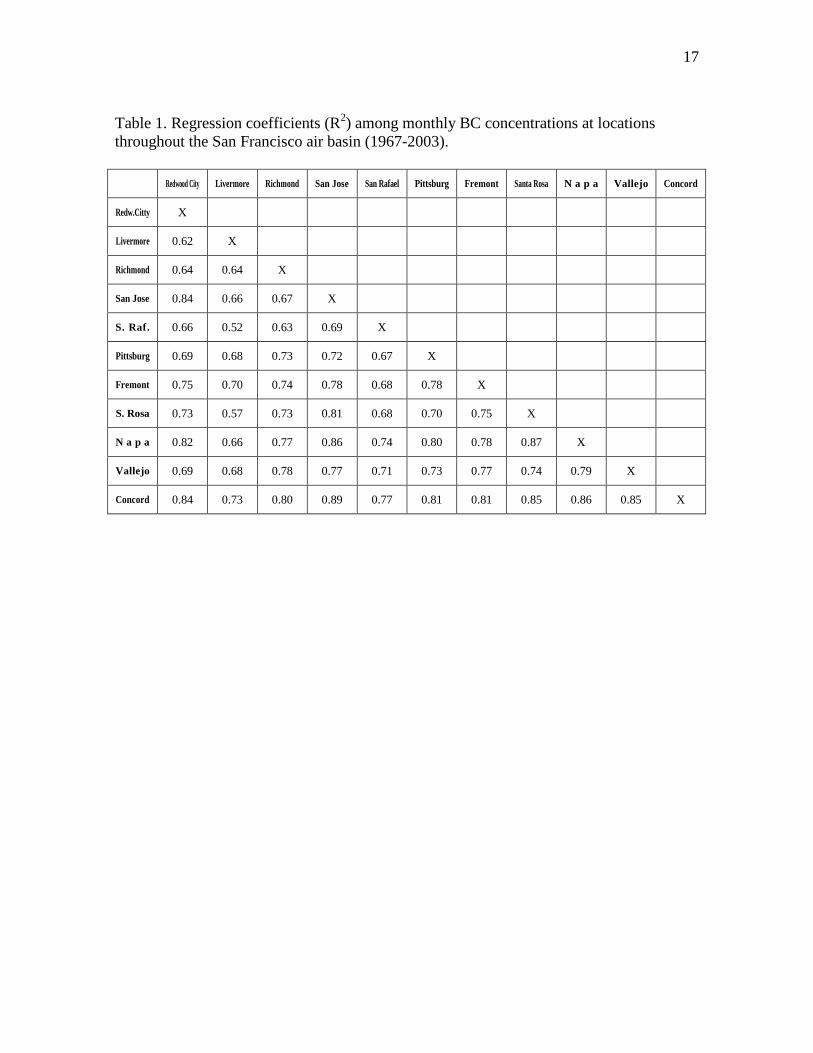
generally between 0.65 and 0.85 (Table 1).
The seasonal cycle in BC concentrations is most likely due to reduced pollutant
dispersion during winter months. Glen et al. [1996] reported lower mean mixing height
(570 vs. 660 m) and mean wind speed (3.7 vs. 6.4 m s-1) in winter months than in summer
months for the San Francisco area. The inter-site correlations in Table 1 indicate that
changes in pollutant dispersion occur synchronously throughout the Bay Area. In contrast
to seasonal variation in pollutant dispersion, motor vehicle fuel consumption, including
diesel, is essentially constant throughout the year [FHA, 2007].
A similar seasonal trend in carbon particle concentrations was observed by Cass et
al. [1984] at seven locations in the Los Angeles area (1958 to mid-1981). They attributed
the seasonality in concentration to decreased atmospheric dispersion during the late fall
and early winter rather than to temporal changes in the emissions from the principal BC
sources, namely diesel vehicles. Diesel vehicle emissions of BC were considered to be
approximately constant throughout the year, as indicated by fuel consumption data [FHA,
2007]. Likewise, Glen et al. [1996] demonstrated that meteorologically driven dispersion,
7
not seasonal variation in emissions, caused the same seasonal trend in carbon monoxide
concentrations in several urban locations, including the San Francisco air basin.
While meteorology likely dominates the seasonal trend in Bay Area BC
concentrations, we considered that increased residential wood burning in the wintertime
[Fairley, 2006] might also be a factor. Schauer and Cass [2000] discuss an extreme wood
smoke event in Fresno (located south of the San Francisco Bay Area), which offers an
upper bound for the contribution of wood burning to ambient BC concentrations. For that
highest wood smoke event, a source apportionment indicated that diesel vehicles and wood
burning, respectively, contributed 80 and 20% of the ambient BC. Thus, the typical BC
contribution from wood burning in the wintertime is likely substantially lower than 20%.
Note that the seasonality in BC concentrations is opposite that of photochemical air
pollutants, most notably ozone. In the summertime, increased solar insolation (and thus
photochemistry) and higher temperatures lead to peak ozone concentrations. While the
population’s health risk due to ozone exposure is at maximum in the summertime [Tager et
al., 2005 and references therein], its exposure-related risk to (toxic and carcinogenic)
diesel emissions, as indicated by increased BC concentrations, is at a maximum in the
wintertime, primarily because of the meteorology of this region.
3.4 Historical trends in BC concentrations and estimated on-road diesel vehicle
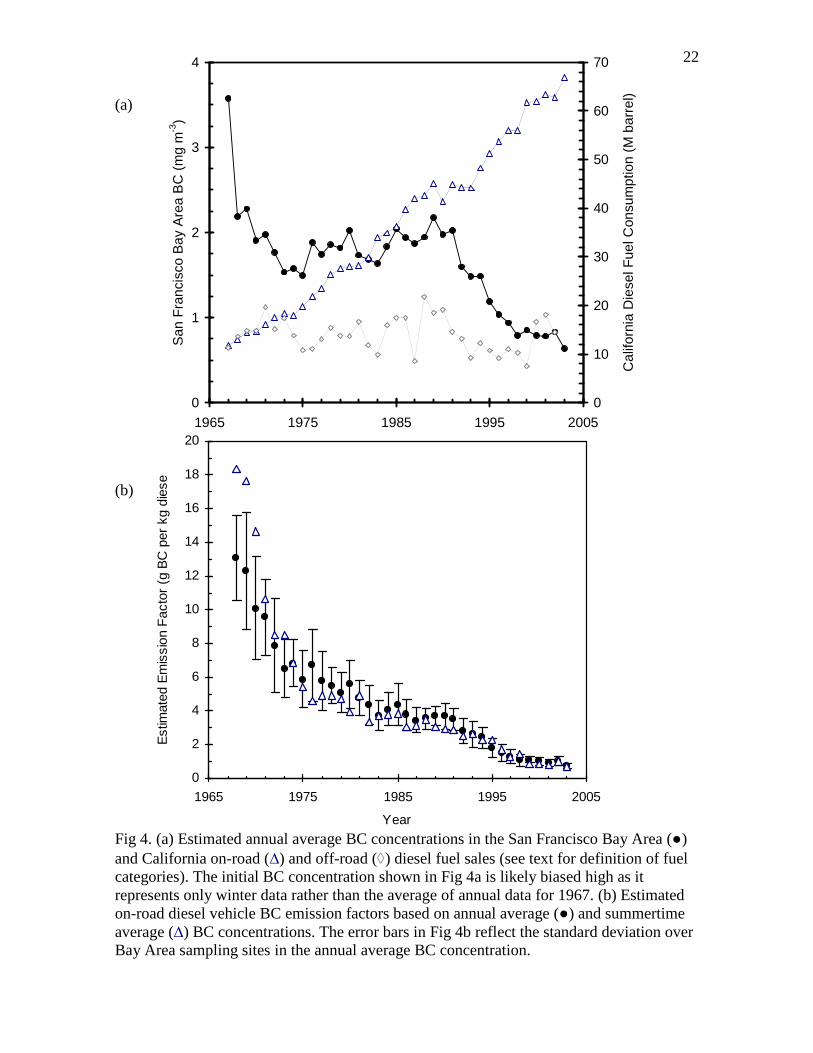
emission factors. Annual average BC concentrations in the Bay Area over the 1967 to
2003 period are shown in Fig. 4a. Annual diesel fuel consumption by on-road motor
vehicles in California is also shown for comparison. Taxable fuel sales are used to measure
on-road vehicle fuel consumption [Cal BOE, 2007]. While diesel fuel use, the main source
of BC emissions, increased by a factor of ~6, BC concentrations decreased by a factor of
~3 over the same period. (The estimated BC concentration in 1967 is likely biased high
because COH data were available only for winter months at many of the active sampling
locations that year.) The contrast in the trends in BC concentration and diesel fuel use is
striking, especially beginning in the early 1990s when BC concentrations began markedly
decreasing despite sharply rising diesel fuel consumption. This contrast suggests that
technology changes to reduce BC emissions have been successful.
Assuming that diesels have been the only significant BC source in the Bay Area,
estimated BC emission factors – the mass of BC emitted per mass of diesel consumed – for
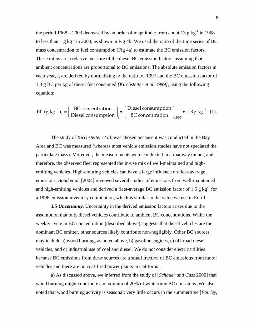
8
the period 1968 – 2003 decreased by an order of magnitude: from about 13 g kg-1 in 1968
to less than 1 g kg-1 in 2003, as shown in Fig 4b. We used the ratio of the time series of BC
mass concentration to fuel consumption (Fig 4a) to estimate the BC emission factors.
These ratios are a relative measure of the diesel BC emission factors, assuming that
ambient concentrations are proportional to BC emissions. The absolute emission factors in
each year, i, are derived by normalizing to the ratio for 1997 and the BC emission factor of
1.3 g BC per kg of diesel fuel consumed [Kirchstetter et al. 1999] , using the following
equation:
-1
ii
-1 kg g ionconcentrat BC
nconsumptio Diesel
nconsumptio Diesel
ionconcentrat BC)kg (g BC 3.1
1997
••=
(1).
The study of Kirchstetter et al. was chosen because it was conducted in the Bay
Area and BC was measured (whereas most vehicle emission studies have not speciated the
particulate mass). Moreover, the measurements were conducted in a roadway tunnel, and,
therefore, the observed fleet represented the in-use mix of well-maintained and high-
emitting vehicles. High-emitting vehicles can have a large influence on fleet-average
emissions. Bond et al. [2004] reviewed several studies of emissions from well-maintained
and high-emitting vehicles and derived a fleet-average BC emission factor of 1.5 g kg-1 for
a 1996 emission inventory compilation, which is similar to the value we use in Eqn 1.
3.5 Uncertainty. Uncertainty in the derived emission factors arises due to the
assumption that only diesel vehicles contribute to ambient BC concentrations. While the
weekly cycle in BC concentration (described above) suggests that diesel vehicles are the
dominant BC emitter, other sources likely contribute non-negligibly. Other BC sources
may include a) wood burning, as noted above, b) gasoline engines, c) off-road diesel
vehicles, and d) industrial use of coal and diesel. We do not consider electric utilities
because BC emissions from these sources are a small fraction of BC emissions from motor
vehicles and there are no coal-fired power plants in California.
a) As discussed above, we inferred from the study of [Schauer and Cass 2000] that
wood burning might contribute a maximum of 20% of wintertime BC emissions. We also
noted that wood burning activity is seasonal; very little occurs in the summertime [Fairley,
9
2006]. In order to remove uncertainty related to emissions from this source, we derived BC
emission factors using summertime BC concentrations (i.e., BC concentrations estimated
from July through August COH data). This revised estimate of BC emission factors
(shown as open triangles in Fig 4b) is very similar to the estimate based on annual BC
concentrations. Thus, emissions from wood burning do not significantly affect our derived
diesel vehicle BC emission factors.
b) The relative importance of BC emissions from gasoline-powered motor vehicles
was estimated from published emission factors. While the BC emission factor from diesel
vehicles is approximately 40 times larger than from gasoline vehicles, roughly six times
more gasoline than diesel fuel is sold in California [Kirchstetter et al. 1999]. Based on BC
emission factors, fuel use, and fuel properties reported in Kirchstetter et al., we estimate
that gasoline engines contribute about 14% of on-road BC emissions, which are not
included in our emission factor calculations. The relative importance of BC emissions from
gasoline vehicles may have been greater earlier in the study period if gasoline engines were
previously much larger BC emitters.
c) The off-road transport sector consists of off-highway vehicles, farming
equipment, rail, and ships. Over the US as a whole it contributes a significant fraction of
BC emissions. [Bond et al. 1994]. We do not expect emissions from farming equipment to
contribute substantially to the San Francisco Bay Area because the major agricultural areas
of California lie downwind of the Bay Area. Consumption of diesel fuel in California from
off-highway vehicles, rail and ships has remained relatively constant compared to on-road
diesel consumption, as shown in Fig 4a. (Due to data unavailability, off-road consumption
in Fig 4a includes off-highway vehicle consumption only after 1983.) Since off-road
diesels are subject to fewer regulations than on-road diesels, the present-day BC emission
factor of off-road diesels is likely higher than that of regulated on-road diesels and has
likely remained relatively constant compared to that of on-road diesels. Bond et al.
summarized available off-road emission factor data and reported central values ranging
from 1.2 to 3.6 gBC kg-1. If the statewide fuel trends shown in Fig 4a apply to the Bay
Area, then based on these emission factors, off-road diesels contribute appreciably to Bay
Area BC concentrations.
10
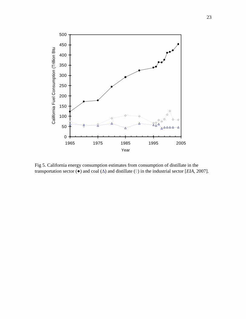
d) While estimates for the United States indicate that BC emissions from industry
are presently a small fraction of those from transportation [Bond et al. 2004], coal and
diesel fuel consumption data for California indicate that industrial BC emissions may have
been more important early in the study period [EIA, 2007]. (By comparison, residential and
commercial consumption of diesel and coal has been negligible. Energy consumption in
these sectors is primarily from natural gas, which contributes negligible amounts of BC.)
Similar to off-road diesel consumption, consumption in the industrial sector has remained
approximately constant throughout the study period, as shown in Fig 5.
In summary, in light of potentially significant BC emissions from other combustion
sources in the Bay Area, the emission factors in Fig 4b may overstate the emissions from
on-road diesels and their historical decrease. Estimating the magnitude of the uncertainty
in emission factors is not possible without additional region-specific fuel consumption
data. While it is reasonable to assume that diesel vehicle BC emissions might have had the
most influence on measured COH concentrations – because monitoring facilities are
influenced by local traffic and several were close to freeways – it is probable that the
values in Fig 4b are upper bounds of the BC emission factors from on-road diesels.
Uncertainty also arises from our assumption that the diesel fuel consumption trend
in the San Francisco Bay Area is the same as the statewide trend. Significant differences
between Bay Area and statewide diesel consumption trends would result in either an over-
or under-stated reduction the derived BC emission factors.
Last, we note that note our assumption of a constant relationship between COH and
BC (i.e., a constant conversion factor) introduces some uncertainty. We assumed a constant
relationship because the concurrent COH and BC data cover a short period of time. If the
relationship varied over the study period, the estimated BC concentrations and emission
factors would be affected. Note that whereas that the estimated BC concentrations depend
on the value of the conversion factor, the emission factors depend only on the trend in the
BC concentrations. Therefore, uncertainty in the magnitude of the conversion factor,
assuming it is constant over time, does not add to the uncertainty the derived emission
factors.
In general the assumptions discussed above become more tenuous farther back in
time and lead to greater uncertainty in the estimated BC emission factors early in early
11
study period. Conversely, the estimated BC emission factors late in the study period, and
the attribution of the decrease in BC concentrations since 1990 to cleaner diesels, probably
carry less uncertainty.
3.6 Reconciliation of estimated BC emission factors with emission regulations
and vehicle emission measurements. Three periods are evident in the changing BC
emission factors and ambient concentrations over the 1967 to 2003 period: (i) pre 1975
when a substantial decrease in emission factors and ambient concentrations occurred, (ii)
1975 – 1990, a period with a gradual decrease in emission factors and approximately level
ambient BC concentrations, and (iii) post 1990 when emission factors and ambient
concentrations again decreased markedly. These three time segments qualitatively
correspond to the following major milestones in emission control policy described by
Lloyd and Cackette [2001].
The first diesel emission controls were directed to visible smoke reduction by
national standards introduced in 1970. Diesel fuel composition, including sulfur content
reduction, changed concurrently with smoke controls. These changes roughly correspond
to the pre-1975 decreases in ambient BC concentrations and emission factors. Diesel
particulate matter emissions, of which BC is the majority, were subsequently controlled
mostly through improvements in engine design. On road heavy-duty diesel particulate
matter emission standards were first implemented in California in 1973. On-road emissions
were reduced as new vehicles replaced older more polluting vehicles. These developments
correspond to the more-gradual decreasing trend in BC emission factors between 1975 and
1990.
In addition to engine improvements through fleet turnover, emission controls and
fuel changes likely contributed to the sharp decrease in BC concentrations and emission
factors after 1990. In the 1990s, many urban transit buses were retrofitted with oxidation
catalysts to reduce PM and, consequently, BC emissions. In 1993, California limited the
sulfur content in diesel fuel to 500 ppm compared to a pre-regulation average of 2500 ppm
and limited aromatic hydrocarbon content to 10%. The data in Fig 4 indicate that BC
concentrations and emission factors decreased following the 1993 regulations. Reducing
the aromatic fuel content is expected to reduce BC emissions. The reduction in fuel sulfur
may also have reduced BC emissions because high fuel sulfur promotes soot formation.
12
Sulfur oxides produced in combustion catalyze the recombination of O and OH radicals,
reduce the degree of acetylene oxidation and thus enhance the formation of soot
precursors; see for example Smith [1981] and references therein. McKenzie et al. [2005]
showed that lowering the fuel sulfur content from 500 ppm to 50 ppm greatly reduced
emissions of polycyclic aromatic hydrocarbons (PAH) from heavy-duty diesel buses.
Although BC emissions were not measured in that study, similar reduction of BC can be
expected because PAH and BC are both products of incomplete combustion and are often
highly correlated [Westerdahl et al. 2005].
A number of vehicle emission studies corroborate technology-driven emission
improvements. Prucz et al. [2001] reported that changing diesel engine technology since
the early 1990s markedly reduced particulate matter emissions. Heavy-duty diesel vehicle
chassis dynamometer tests indicate that particulate matter emission factors trend downward
with engine model year: emission factors from 1995 and newer models were ten times less
than emissions from pre 1980 models [CRC, 2003]. The introduction of new technology by
way of fleet turnover resulted in measured decreases in on-road diesel particulate matter
and BC emissions factors of 48 and 39%, respectively, between 1997 and 2006 [Ban-Weiss
et al. 2007].
3.7 Recommended BC measurements. We restate the need for additional side-by-
side measurements of COH and BC and recommend increased routine monitoring of BC.
There are few collocated COH and BC measurements and, as noted above, more would
strengthen the relationship between COH and BC derived in this study. Routine monitoring
of BC is needed to continue tracking ambient concentrations. The COH monitoring
network in California has been retired without replacement.
Acknowledgements
This work was supported by the California Energy Commission’s Public Interest
Energy Research program, and the Director, Office of Science, Office of Biological and
Environmental Research, U.S. Department of Energy. The NARSTO aethalometer BC data
was obtained from the NASA Langley Research Center Atmospheric Science Data Center.
We thank Eric Stevenson and Stanley Yamaichi of the BAAQMD for providing helpful

13
information about COH sampling in the Bay Area. We also thank the anonymous peer
reviewer for his/her helpful comments.
14
References
Allen, G. A, J. Lawrence, and P. Koutrakis, (1999), Field validation of a semi-continuous method for aerosol black carbon (aethalometer) and temporal patterns of summertime hourly black carbon measurements in southwestern PA, Atmos. Environ. 33, 817–823.
ARB (2003), http://www.arb.ca.gov/diesel/diesel.htm BAAQMD, Bay Area Air Quality Management District (2006), Spare the air tonight study,
2005-2006 winter wood smoke season. Report conducted for BAAQMD by True North Research, Encinitas, California, available online: http://www.sparetheair.org/about/2005-winter-report.pdf.
Bond, T.C., D.G. Street, K.F. Yarber, S.M. Nelson, J._H. Woo, and Z. Klimont, A technology-based global inventory of black and organic carbon emissions from combustion, J. Geophys. Res., 109, D14203, doi: 10/1029/2003JD003697, 2004.
Cal BOE, California Board of Equalization, http://www.boe.ca.gov/annual/statindex0405.htm, Table 25A. Taxable distributions of diesel fuel and alternative fuels, effective March 2007.
Cal EPA, California Environmental Protection Agency, “Chemicals known to the state to cause cancer or reproductive toxicity,” http://www.oehha.ca.gov/prop65/prop65_list/files/P65single052005.pdf, Proposition 65 list of chemicals, effective May 2005.
CARB, California Air Resources Board, http://www.arb.ca.gov/aqd/aqdcd/aqdcd.htm, California air quality data CD, released in 2006.
CARB, California Air Resources Board, Proposed identification of diesel exhaust as a Toxic Air Contaminant. AppendixIII, PartA, ExposureAssessment. ARB, Sacramento, CA, 1998.
Cass, G.R., M. H. Conklin, J. J. Shah, J. J. Huntzicker, and E. S. Macias, (1984), Elemental carbon concentrations: Estimationof an historical data base, Atmos. Environ., 18, 153-162.
CEC, California Energy Commission (1997) Energy Watch, The CEC’s summary of energy trends in California, Volume 16, Data through December 1994. Available online, http://www.energy.ca.gov/reports/energywatch-16/.
Chinkin, LR; Coe, DL; Funk, TH; Hafner, HR; Roberts, PT; Ryan, PA; Lawson, DR. (2003) Weekday versus weekend activity patterns for ozone precursor emissions in California's South Coast Air Basin, J. Air Waste Manage. Assoc., 53, 829–843
Cooke, W. F., C. Liousse, H. Cachier, and J. Feichter (1999), Construction of a 1° × 1° fossil fuel emission data set for carbonaceous aerosol and implementation in the ECHAM4 model (1999), J. Geophys. Res., 104 (D18), 22,137–22,162.
CRC, Coordinating Research Council (2003) Statistical Analysis of CRC E-55/E-59 Phase 1 Data, Available online, http://www.crcao.com/reports/recentstudies2003/E-71CompleteReport030301.pdf
Dreher, D.B.; Harley, R.A. A Fuel-Based Inventory for Heavy-Duty Diesel Truck Emissions. J. Air & Waste Manag. Assoc., 48, 352-358, 1998.
EIA, Energy Information Administration (2007) State Energy Data 2004: Consumption, 1960-2004, California. Available online, http://www.eia.doe.gov/emeu/states/state.html?q_state_a=ca&q_state=CALIFORNIA.
15
Fairley, D., Revised Estimates of Wood Burning in the San Francisco Bay Area, Draft Report for the Bay Area Air Quality Management District, 2006.
FHA, Federal Highway Administration (2007), Monthly motor fuel reported by states, Report series is available online, http://www.fhwa.dot.gov/ohim/mmfr/dec02/index.htm.
Fruin, SA; Winer, AM; Rodes, CE, Black carbon concentrations in California vehicles and estimation of in-vehicle diesel exhaust particulate matter exposures, Atmos. Environ., 38, 4123-4133, 2004.
Glen, WG; Zelenka, MP; Graham, RC. Relating meteorological variables and trends in motor vehicle emissions to monthly urban carbon monoxide concentrations, Atmos. Environ., 30, 4225-4232, 1996.
Hansen, ADA; Rosen, H; Novakov, T. The aethalometer – an instrument for the real-time measurement of optical absorption by aerosol particles, Sci. Tot. Environ., 36, 191-196, 1984
Hansen, J.; Bond, T.; Cairns, B.; Gaeggler, H.; Liepert, B.; Novakov, T.; Schichtel, B. (2005) Carbonaceous Aerosols in the Industrial Era. EOS, 85, 241-248.
Harley, RA; Marr, LC; Lehner, JK; Giddings, SN (2005) Changes in motor vehicle emissions on diurnal to decadal timescales and effects on atmospheric composition, Environ. Sci. Technol., 39, 5356–5362.
Horvath, H. Atmospheric light absorption – a review. Atmos. Environ., 27A, 293-317, 1993
Hemeon, W.C.L., G.F. Haines, and H.M. Ide (1953), Determinationof haze and smoke concentrations by filter paper samples, Air Repair 3, 22–28.
Houghton, J. T.; Y. Ding, D. J. Griggs, M. Noguer, P. J. van der Linden, and S. Xiaosu, Climate change 2001: the scientific basis, Cambridge University Press, Cambridge, 2001.
Ito, A., and J. E. Penner (2005), Historical emissions of carbonaceous aerosols from biomass and fossil fuel burning for the period 1870–2000, Global Biogeochem. Cycles, 19, GB2028, doi:10.1029/2004GB002374.
Jacobson, M.Z. Strong radiative heating due to the mixing state of black carbon in atmospheric aerosols. Nature, 409, 695-697, 2001.
Kandlikar, M., and G. Ramachandran, (2000), The causes and consequences of particulate air pollution in urban India: A synthesis of the science, Annu. Rev. Energy Environ., 25, 629-684.
Kirchstetter, T.W., R. A. Harley, N. M. Kreisberg, M. R. Stolzenburg, and S. V. Hering, (1999), On-road measurement of the particle and nitrogen oxide emissions from light- and heavy-duty motor vehicles, Atmos. Environ., 33, 2955-2968.
Lloyd, A.C., and T. A. Cackette (2001), Diesel engines: Environmental impact and control, J. Air & Waste Manage. Assoc., 51, 809-847
Lough, GC; Schauer, JJ; Lawson, DR. (2006) Day of week trends in carbonaceous aerosol concentration in the urban atmosphere, Atmos. Environ., 40, 4137-4149.
Marr, LC; Black, DR; Harley, RA. (2002). Formation of photochemical air pollution in central California. 1. Development of a revised motor vehicle emission inventory. J. Geophys. Res., 107, doi: 10.1029/2001JD000689
McKenzie, C. H., L. Godwin, A. Ayoko, L. Morawska, Z. D. Ristovski, and E. R. Jayaratne, (2005), Effect of fuel composition and engine operating conditions on
16
polycyclic aromatic hydrocarbon emissions from a fleet of heavy-duty diesel buses, Atmos. Environ., 39, 7836–7848.
Motallebi, N; Tran, H; Croes, BE; Larsen, LC. (2003) Day-of-week patterns of particulate matter and its chemical components at selected sites in California, J. Air Waste Manage. Assoc., 53, 876–888.
NARSTO, Single wavelength aethalometer data from the EPA supersite in Fresno, California, http://eosweb.larc.nasa.gov/cgi-bin/searchTool.cgi?Dataset=NARSTO_EPA_SS_FRESNO_EC_PM25_FRACTION, effective 2007.
Novakov, T.; Hansen, JE. (2004) Black carbon emissions in the United Kingdom during the past four decades: an empirical analysis, Atm. Environ., 38, 4155–4163.
Novakov, T., V. Ramanathan, J. E. Hansen, T. W. Kirchstetter, M. Sato, J. E. Sinton, and J. A. Sathaye, (2003), Large historical changes of fossil-fuel black carbon aerosols, Geophys. Res. Letters, 30, NO. 6, 1324, doi:10.1029/2002GL016345.
NJ DEP, New Jersey Department of Environmental Protection, http://www.state.nj.us/dep/airmon/part01.pdf, 2001 air quality report, 2001 particulate summary, effective March 2007.
Pope, CA; Dockery, DW. (2006) Health effects of fine particulate air pollution: lines that connect, J. Air Waste Manage. Assoc., 56, 709-742.
Prucz, JC; Clark, NN; Gautam, M; Lyons, DW (2001), Exhaust emissions from engines of the Detroit Diesel Corporation in transit buses: a decade of trends, Environ. Sci. Tech., 35, 1755-1764.
Schauer, JJ; Cass, GR; Simoneit, BRT (2000) Source apportionment of wintertime gas-phase and particle-phase air pollutants using organic compounds as tracers, Environ. Sci. Technol., 34, 1821-1832.
Smith, O. I. (1981), Fundamentals of soot formation in flames withapplication to diesel engine particulate emissions, Prog. Energy Combust. Sci., 7, 275-291.
Tager, IB; Balmes, J; Lurmann, F; Ngo, L; Alcorn, S; Kunzli, N. Chronic exposure to ambient ozone and lung function in young adults, Epidemiology, 16, 751-759, 2006.
Westerdahl, D; Fruin, S; Sax, T; Fine, PM; Sioutas, C. Mobile platform measurements of ultrafine particles and associated pollutant concentrations on freeways and residential streets in Los Angeles, Atmos. Environ., 39, 3597-3620, 2005.
Yamaichi, S;.Stevenson, E. (2007) Personal communication with members of the Technical Services Division of the Bay Area Air Quality Management District.
17
Table 1. Regression coefficients (R2) among monthly BC concentrations at locations throughout the San Francisco air basin (1967-2003).
Redwood City Livermore Richmond San Jose San Rafael Pittsburg Fremont Santa Rosa N a p a Vallejo Concord
Redw.Citty X
Livermore 0.62 X
Richmond 0.64 0.64 X
San Jose 0.84 0.66 0.67 X
S. Raf. 0.66 0.52 0.63 0.69 X
Pittsburg 0.69 0.68 0.73 0.72 0.67 X
Fremont 0.75 0.70 0.74 0.78 0.68 0.78 X
S. Rosa 0.73 0.57 0.73 0.81 0.68 0.70 0.75 X
N a p a 0.82 0.66 0.77 0.86 0.74 0.80 0.78 0.87 X
Vallejo 0.69 0.68 0.78 0.77 0.71 0.73 0.77 0.74 0.79 X
Concord 0.84 0.73 0.80 0.89 0.77 0.81 0.81 0.85 0.86 0.85 X
18
Figure Captions Fig 1. Collocated monthly average BC (aethalometer) and COH levels in Fresno, CA during the North American Research Strategy for Tropospheric Ozone study [NARSTO 2007]. Also shown is the linear regression line reported by Allen et al. [1999] for measurements in Philadelphia, PA. Fig 2. Average Bay Area BC concentrations by day of week over the period 1967 to 2003 (a) averaged over the whole year and (b) averaged for each month of the year. The error bars reflect the relative standard deviation over sampling sites in the daily average BC concentration. Fig 3. (a) Monthly BC concentrations (COH also shown), averaged for 11 locations in the San Francisco Bay area from 1980 to 1990. (b) Annual trend in BC over the period 1967-2003 at each location. Average monthly concentrations are normalized to June. Fig 4. (a) Estimated annual average BC concentrations in the San Francisco Bay Area (●) and California on-road (∆) and off-road (◊) diesel fuel sales (see text for definition of fuel categories). The initial BC concentration shown in Fig 4a is likely biased high as it represents only winter data rather than the average of annual data for 1967. (b) Estimated on-road diesel vehicle BC emission factors based on annual average (●) and summertime average (∆) BC concentrations. The error bars in Fig 4b reflect the standard deviation over Bay Area sampling sites in the annual average BC concentration. Fig 5. California energy consumption estimates from consumption of distillate in the transportation sector (●) and coal (∆) and distillate (◊) in the industrial sector [EIA, 2007].
19
Fig 1. Collocated monthly average BC (aethalometer) and COH levels in Fresno, CA during the North American Research Strategy for Tropospheric Ozone study [NARSTO 2007]. Also shown is the linear regression line reported by Allen et al. [1999] for measurements in Philadelphia, PA.
y = 5.13x + 0.57R2 = 0.96
0
1
2
3
4
5
6
0.0 0.2 0.4 0.6 0.8 1.0
Coefficient of Haze (COH)
Aet
halo
met
er B
lack
Car
bon
( µg
m-3
)Fresno, CA (NARSTO)
Philadelphia (Allen et al. 1999)
y = 5.66x - 0.26R2 = 0.99
20
(a) (b) Fig 2. Average Bay Area BC concentrations by day of week over the period 1967 to 2003 (a) averaged over the whole year and (b) averaged for each month of the year. The error bars reflect the relative standard deviation over sampling sites in the daily average BC concentration.
1.0
1.1
1.2
1.3
1.4
1.5
1.6
1.7
1.8
1.9
2.0
1 2 3 4 5 6 7 1 2 3 4 5 6 7 1 2 3 4 5 6 7 1 2 3 4 5 6 7 1 2 3 4 5 6 7 1 2 3 4 5 6 7 1 2 3 4 5 6 7 1 2 3 4 5 6 7 1 2 3 4 5 6 7 1 2 3 4 5 6 7 1 2 3 4 5 6 7 1 2 3 4 5 6 7
jan feb mar apr may jun jul aug sep oct nov dec
Day of Week (Sunday = 1) and Month of Year
Dai
ly A
vera
ge B
C (
Nor
mal
ized
to S
unda
y)
1.0
1.2
1.4
1.6
1 2 3 4 5 6 7
Day of Week (Sunday = 1)
Dai
ly A
vera
ge B
C (
Nor
mal
ized
to S
unda
y)
21
(a) (b) Fig 3. (a) Monthly BC concentrations (COH also shown), averaged for 11 locations in the San Francisco Bay area from 1980 to 1990. (b) Annual trend in BC over the period 1967-2003 at each location. Average monthly concentrations are normalized to June.
0
1
2
3
4
5
6
Jan-80
Jan-81
Jan-82
Jan-83
Jan-84
Jan-85
Jan-86
Jan-87
Jan-88
Jan-89
BC
(µg
m-3
)
0.0
0.2
0.4
0.6
0.8
1.0
CO
H
1.0
1.5
2.0
2.5
3.0
3.5
4.0
4.5
5.0
5.5
1 2 3 4 5 6 7 8 9 10 11 12
Month of Year (1=January)
Mon
thly
Ave
rage
BC
(N
orm
aliz
ed to
Jun
e)
1.0
1.5
2.0
2.5
3.0
3.5
4.0
4.5
5.0
5.5Vallejo
Napa
Concord
Santa Rosa
San Jose
Pittsburg
Redwood City
San Rafael
Livermore
Fremont
Richmond
22
(a) (b) Fig 4. (a) Estimated annual average BC concentrations in the San Francisco Bay Area (●) and California on-road (∆) and off-road (◊) diesel fuel sales (see text for definition of fuel categories). The initial BC concentration shown in Fig 4a is likely biased high as it represents only winter data rather than the average of annual data for 1967. (b) Estimated on-road diesel vehicle BC emission factors based on annual average (●) and summertime average (∆) BC concentrations. The error bars in Fig 4b reflect the standard deviation over Bay Area sampling sites in the annual average BC concentration.
0
1
2
3
4
1965 1975 1985 1995 2005
San
Fra
ncis
co B
ay A
rea
BC
(m
g m
-3)
0
10
20
30
40
50
60
70
Cal
iforn
ia D
iese
l Fue
l Con
sum
ptio
n (M
bar
rel)
0
2
4
6
8
10
12
14
16
18
20
1965 1975 1985 1995 2005
Year
Est
imat
ed E
mis
sion
Fac
tor
(g B
C p
er k
g di
esel
)
`
23
Fig 5. California energy consumption estimates from consumption of distillate in the transportation sector (●) and coal (∆) and distillate (◊) in the industrial sector [EIA, 2007].
0
50
100
150
200
250
300
350
400
450
500
1965 1975 1985 1995 2005
Year
Ca
lifo
rnia
Fu
el C
on
sum
ptio
n (
Tril
lion
Btu
)