Perturbative quantum consistency near black-hole horizon formation

Stefan Hofmann∗ and Maximilian Koegler†

Arnold Sommerfeld Center for Theoretical Physics, Theresienstraße 37, 80333 Munchen, Germany

Florian Niedermann‡

Nordita, KTH Royal Institute of Technology and Stockholm UniversityHannes Alfvens vag 12, SE-106 91 Stockholm, Sweden

(Dated: December 13, 2021)

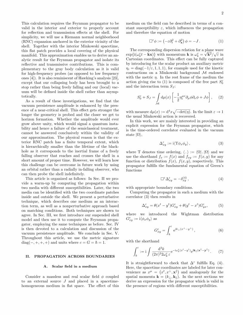
We study the prelude to black-hole formation using a suspended shell composed of physical matterthat fulfills the dominant energy condition. Here, the collapse of the shell is brought to rest whenthe formation of the horizon is imminent but has not yet occurred. As the main achievement of thiswork, we obtain the Feynman propagator which connects the interior and the exterior of the shellwithin two local coordinate patches. It is derived by drawing an analogy to the propagation of lightacross interfaces that separate regions with different susceptibilities inside a medium. As a firstapplication, we use this propagator to determine the vacuum persistence amplitude in the presenceof external sources. On timescales much shorter than the Page time, we find that the amplitudebuilds up with time yet remains consistent with perturbative unitarity.

I. INTRODUCTION

In recent years, observations have been able to testour understanding of black-holes with increasing accu-racy. For example, the gravitational wave signal froma binary black-hole merger provides us with informationabout their masses and intrinsic vibrational modes [1];similarly, the event horizon telescope [2] probes the clas-sical geometry close to the event horizon. While all ofthese observations have been compatible with the pre-diction from general relativity, deep theoretical problemsremain beyond the classical level. Most prominently, theinformation paradox arises from a semiclassical analysisof the formation and evaporation process of a black-hole.In a nutshell, it is based on the observation that an ini-tially pure quantum state that collapses into a black-holeevolves into a mixed state after the black-hole has evap-orated [3], in contradiction to a consistent, unitary timeevolution.

In this work, we study the quantum consistency of athin-shell system close to black-hole formation. To thisend, we will pursue a very conservative approach wherewe employ the standard semiclassical toolkit. This willavoid complications arising from the presence of a hori-zon, yet allow us to adiabatically probe the quantum sta-bility of the shell system while it approaches a black-holestate. In other words, we start out with a configurationthat is paradox-free and very slowly move toward horizonformation. We then ask if we can find any direct evidencefor a buildup of quantum corrections that would indi-cate the breakdown of the semiclassical approximation.This could be hinting at a nonperturbative descriptionof black-holes [4–7] as it has also been suggested throughexplicit constructions in the literature [8–19].

∗ Stefan.Hofmann@physik.uni-muenchen.de† M.Koegler@physik.uni-muenchen.de‡ Florian.Niedermann@su.se

Our proposal faces two immediate challenges. First,we have to come up with a physical model that admitsan arbitrarily slow collapse. In particular, we cannotuse standard collapse models where for typical black-holemasses the near-horizon regime as seen by a comovingobserver is passed within microscopic timescales. Second,we have to find a sufficiently simple diagnostic tool, whichenables us to probe the quantum evolution of fields onthe shell background over long enough time intervals tobe sensitive to accumulated growth effects.

We overcome the first challenge by introducing a sus-pended shell model. Here, the idea is to stabilize a mas-sive, nonrelativistic shell with surface density ρ throughits surface pressure p, which we treat as a free parame-ter. Provided the shell radius R is slightly larger thanthe Schwarzschild radius rg, explicitly R > 25rg/24, wefind that the shell can be brought to a complete stopwhile still being composed of matter fulfilling the strongand dominant energy condition. In such a static model,we can treat R as a free dial to probe different stages ofblack-hole formation.

Regarding the second challenge, we will study thepropagation of a quantum scalar field on the gravita-tional shell background. Specifically, we will calculatefor an inertial observer the persistence amplitude of theMinkowski vacuum inside the shell in the presence of anexternal source [20]. In particular, this diagnostic toolis sensitive to effects that buildup over time and couldbe missed in a standard stability perturbative analysis.1

1 In [6] and [7] a similar objective was pursued by studying seculargrowth close to Schwarzschild and Rindler horizons, respectively.Also, see [21] for a more recent work where coherent states arecollapsed into black-holes. In contrast, our work has its focus onthe Minkowski vacuum in the interior of the shell (rather than theasymptotic one) and our shell – as seen by a comoving observer –is prevented from crossing the horizon. For a specific microscopicrealization of a suspended shell in the context of string theorysee [22].

arX

iv:2

109.

0324

2v2

[he

p-th

] 9

Dec

202

1

2

This calculation requires the Feynman propagator to bevalid in the interior and exterior to properly accountfor reflection and transmission effects at the shell. Forsimplicity, we will use a Riemann normal neighborhood(RNC) expansion anchored in the exterior vicinity of theshell. Together with the interior Minkowski spacetime,this flat patch provides a local covering of the physicalmanifold. This approximation enables us to derive an an-alytic result for the Feynman propagator and isolate itsreflective and transmissive contributions. This is com-plementary to the gray body calculation as it is validfor high-frequency probes (as opposed to low frequencyones [4]). It is also reminiscent of Hawking’s analysis [23],except that our collapsing body has been brought to astop rather than being freely falling and our (local) vac-uum will be defined inside the shell rather than asymp-totically.

As a result of these investigations, we find that thevacuum persistence amplitude is enhanced by the pres-ence of a near-critical shell. This effect gets stronger thelonger the geometry is probed and the closer we get tohorizon formation. Whether the amplitude would evergrow above unity, which would signal a quantum insta-bility and hence a failure of the semiclassical treatment,cannot be answered conclusively within the validity ofour approximation. The physical reason is that the ex-terior RNC patch has a finite temporal extent, whichis hierarchically smaller than the lifetime of the black-hole as it corresponds to the inertial frame of a freelyfalling observer that reaches and crosses the shell in ashort amount of proper time. However, we will learn howthis challenge can be overcome in future work by usingan orbital rather than a radially in-falling observer, whocan then probe the shell indefinitely.

This article is organized as follows: In Sec. II we pro-vide a warm-up by computing the propagation withintwo media with different susceptibilities. Later, the twomedia can be identified with the two coordinate patchesinside and outside the shell. We present a perturbativetechnique, which describes one medium as an interac-tion term, as well as a nonperturbative approach basedon matching conditions. Both techniques are shown toagree. In Sec. III, we first introduce our suspended shellmodel and then use it to compute the Feynman propa-gator, employing the same techniques as before. Sec. IVis then devoted to a calculation and discussion of thevacuum persistence amplitude. We conclude in Sec. V.Throughout this article, we use the metric signaturediag(−,+,+,+) and units where c = G = ~ = 1.

II. PROPAGATION ACROSS BOUNDARIES

A. Scalar field in a medium

Consider a massless and real scalar field φ coupledto an external source J and placed in a spacetime-homogeneous medium in flat space. The effect of this

medium on the field can be described in terms of a con-stant susceptibility ε, which influences the propagationand therefore the equation of motion

εφ :=(−ε∂2

t + ∂2x

)φ = −J . (1)

The corresponding dispersion relation for a plane waveexpi(ωεkt− kx) with momentum k is ωεk =

√k2/√ε in

Cartesian coordinates. This effect can be fully capturedby introducing for the scalar product an auxiliary metricηε = diag(−1/ε, 1, 1, 1), for example used for the kineticcontractions on a Minkowski background M endowedwith the metric η. In the rest frame of the medium theaction giving rise to (1) is composed of the free part Sε0and the interaction term SJ :

Sε0 + SJ =

∫M

dµ(x)

[−1

2ηµνε ∂µφ∂νφ+ Jφ

], (2)

with measure dµ(x) := d4x√−det(η). In the limit ε→ 1

the usual Minkowski action is recovered.In this work, we are mainly interested in providing an

explicit expression for the Feynman propagator, whichis the time-ordered correlator evaluated in the vacuumstate |Ω〉,

∆εxy := i〈Tφxφy〉 , (3)

where T denotes time ordering, 〈 . 〉 := 〈Ω| . |Ω〉 and weuse the shorthand fx := f(x) and fxy := f(x, y) for anyfunction or distribution f(x), f(x, y), respectively. Thispropagator fulfills the fundamental equation of Green’sfunctions

ε∆εxy = −δ(4)

xy , (4)

with appropriate boundary conditions.Computing the propagator in such a medium with the

correlator (3) then results in

∆εxy = θ(xt − yt)Gεxy + θ(yt − xt)Gεyx, (5)

where we introduced the Wightman distributionGεxy := i〈φxφy〉 as

Gεxy =

∫ ε

k

eik⊥(x⊥−y⊥) , (6)

with the shorthand∫ ε

k

:= i

∫d3k

(2π)32ωεk εe−iωεk(xt−yt)eik‖(x

‖−y‖) . (7)

It is straightforward to check that ∆ε fulfills Eq. (4).Here, the spacetime coordinates are labeled for later con-venience as xµ =

(xt, x⊥,x‖

)and analogously for the

spatial momenta k = (k⊥,k‖). In the next sections wederive an expression for the propagator which is valid inthe presence of regions with different susceptibilities.

3

B. Perturbative approach

1. Different dispersion relations encoded as interaction

We first present a perturbative derivation of the prop-agator in systems with boundaries. As an instructiveexample, we consider a spacetime region with domain Sand its complement SC , characterized by the suscepti-bilities εS and ε, respectively. We can think of such asystem as a scattering object S placed in a surround-ing medium SC . The free action of a scalar field in thissystem is given by

S0 = −1

2

∫SC

dµ ηµνε ∂µφ∂νφ−1

2

∫S

dµ ηµνεS ∂µφ∂νφ . (8)

As before, the kinetic terms determine the dispersion re-lation of the scalar field within the scattering object andthe surrounding medium. However, solving the definingequation of the propagator in such a system can becomearbitrarily complicated depending on the geometry of thescattering object.

This difficulty can be circumvented by adopting the fol-lowing viewpoint. We require that the field φ propagateseverywhere according to the first kinetic term in (8); i.e.,we identify it with the free action Sε0 introduced in (2).Since this leads to an error when describing propagationwithin the scattering object, we compensate for this byadding an interaction term SI to the action. This thencorresponds to a formal (but fully equivalent) rewritingof (8); explicitly S0 = Sε0 + SI , where

SI :=

∫S

dµLI := −1

2

∫S

dµ(ηµνεS ∂µφ∂νφ− ηµνε ∂µφ∂νφ

).

(9)

Adopting this perspective, the propagator ∆ε in (5)describes the “free” propagation valid for a uniformmedium with susceptibility ε. The effect of the scatter-ing object is then encapsulated in the interaction termwith Lagrangian LI = λS (∂tφ)

2/2 and coupling con-

stant λS = εS − ε. Employing the interaction picture offield theory, the nonperturbative propagator in the pres-ence of the scattering object, valid everywhere in space,is given by

∆xy = i

⟨Tφxφy e

iλS2

∫S

dµz(∂ztφz)2⟩con

, (10)

where 〈·〉con only includes connected diagrams and as

usual limTz→∞(1+iε)

∫ Tz−Tz dzt is understood. Contrac-

tions of fields in this theory give rise to the propagator∆ε and εS only occurs through the coupling constant λS .

We note that there is a formal symmetry under theexchange of S and SC . This implies that we could haveinstead defined the “free” propagation with respect tothe region S and the effect of the medium in SC in terms

of an interaction term. In this way, ∆εS would havebeen the propagator and ε − εS the coupling constant.While this choice does not matter in the nonperturbativeevaluation (10), it is relevant when (10) is truncated atfinite order in λS .

This is demonstrated by the following example: If wetake the scattering object to cover the whole space, (10)gives rise to a geometric series that can be resummedto ∆εS . This is not surprising, since in the same waya massive propagator can be generated from the resum-mation of the mass term m2φ2 “interactions” [24]. How-ever, if one truncates at a finite order in λS , one doesnot obtain ∆εS , but a propagator which at best approx-imates ∆εS . On the other hand, if one treats the space-time region with susceptibility ε as the interacting part,the integral in (10) has no support and thus vanishes.In this way, ∆εS trivially emerges no matter how manyorders in λS we take into account. Therefore, for thisparticular system, the latter point of view is preferable.Moreover, if the difference between ε and εS is sufficientlysmall, evaluating (10) perturbatively to some order in λSis a viable approach, but fails of course if the difference istoo large. This nonperturbative regime necessarily setsin when |λS | > 1 (or even earlier, as we will see below).

2. Reflection and transmission of a boundary

Demonstrating the effects of a boundary separatingtwo media with different susceptibilities can be bestachieved for the simplest case of two half-spaces. Thescattering object has susceptibility εS and covers the up-per half-space > with spatial domain S =

x : x⊥ > 0

.

Correspondingly, the lower half-space < with domainSC =

x : x⊥ < 0

has susceptibility ε as depicted in

Fig. 1.We can expand (10) for small λS ,

∆xy = ∆εxy + λS

∫S

dµz1 ∂zt1∆εxz1∂zt1∆ε

z1y

+λ2S

∫S

dµz1dµz2 ∂zt1∆εxz1∂zt1∂zt2∆ε

z1z2∂zt2∆εz1y+O

(λ3S

).

(11)

We then use standard field theory methods to furtherevaluate these different tree-level terms. This lengthy butstraightforward calculation is detailed in Appendix A.Fixing the causal arrangement with xt > yt and settingy⊥ < 0 for simplicity, the various contributions to theresummed propagator (or equivalently to the Wightmandistribution) Gxy := ∆xy|xt>yt can be grouped in threeterms,

Gxy = (1− θx⊥)(Gεxy +GRxy

)+ θx⊥G

Txy . (12)

There is a single term Gεxy, as defined in (6), describingdirect propagation from y to x in the lower half-space <.

4

b) Transmission GT

y

xz1

y

xz1

y

x

z2x⊥

0

x‖

a) Reflection GR

>

<

εS

εy x

z1

y x

z1z2

x⊥

0

x‖

1

FIG. 1. The scattering object with susceptibility εS cover-ing the upper half-space > is shaded in gray, the lower half-space < with susceptibility ε in white. The spatial projectionsof the contributions to the reflection propagator GR and thetransmission propagator GT arising from (10) up to secondorder in λS are represented schematically in a) and b), re-spectively.

The two diagrams depicted in Fig. 1a) contribute to thereflection propagator (for x⊥ < 0)

GRxy = −∫ ε

k

eik⊥(x⊥+y⊥)R(ω) , (13)

with reflection coefficient

R(ω) =1

4ω − 1

8ω2 +O

(ω3), (14)

where for convenience we introduced a rescaled expansionparameter ω = λS(ωεk)2/k2

⊥ = λS [1+tan2(α)]/ε with theangle of incidence α defined through k2

‖ =: tan2(α)k2⊥.

The remaining terms, as shown in Fig. 1b), give rise tothe transmission propagator (for x⊥ > 0)

GTxy =

∫ ε

k

eik⊥(x⊥−y⊥)T (ω)

×[

1+i

2

(ω − ω2

4

)k⊥x

⊥− 1

8ω2k2

⊥(x⊥)2 ]

+O(ω3),

(15)

which we have factorized into x⊥ dependent and indepen-dent terms. The latter are collected in the transmissioncoefficient

T (ω) = 1− 1

4ω +

1

8ω2 +O

(ω3)

= 1−R(ω) . (16)

The x⊥ dependent terms, on the other hand, can be re-summed as an exponential, giving rise to the final expres-sion (for x⊥ > 0)

GTxy =

∫ ε

k

eiq⊥x⊥−ik⊥y

⊥T (ω) , (17)

where

q⊥(k) = sgn(k⊥)

√(εSε− 1)k2‖ +

εSεk2⊥ . (18)

The replacement k⊥ → q⊥ ensures that the dispersionrelation inherited from S holds in the upper half-plane,i.e. εSx G

Txy = 0 (whereas εxG

Rxy = 0 in the lower half-

plane).If we want to truncate the ω expansion and work with a

finite number of terms, we must guarantee the smallnessof ω by requiring λS/ε 1 and tan2(α) 1. Therefore,in the perturbative regime, only scenarios with T ≈ 1and R 1 can be consistently described. Since we arelater interested in systems where total reflection can oc-cur, a closed-form expression of this series would be de-sirable. Fortunately, for the case at hand a resummationis feasible and given by

T (ω) =

∞∑n=0

√π

(1 + n)!Γ( 12 − n)

ωn =2

1 +√

1 + ω

= 1−R(ω) , (19)

where Γ denotes the Gamma function. For the firstthree terms in the sum, the Gamma function becomes√π,−2

√π and 4

√π/3 giving the transmission coefficient

as (16).2 The closed-form expression in terms of the an-gle of incidence α is computed to be

R(α) =

√(εSε − 1

)tan2(α) + εS

ε − 1√(εSε − 1

)tan2(α) + εS

ε + 1. (20)

A few remarks are in order. First, the Feyn-man propagators describing reflection and transmis-sion can be obtained as usual by time ordering,

e.g. ∆R|Txy = θ(xt − yt)GR|Txy + θ(yt − xt)GR|Tyx . Second,

identifying the series through the first two orders couldonly be achieved due to the simplicity of the bound-ary. For example for systems with a geometrically morecomplicated boundary one has to stick to the pertur-bative expansion in (11). Third, the resummed re-flection and transmission coefficients fulfill the identityR(ω) + T (ω) = 1 and agree with the spin-averaged Fres-nel equations. They are also correct if λS/ε is large. Infact, total reflection, |R|2 → 1, does occur for εS/ε→∞

2 We have checked this result only up to second order in ω but acomplementary nonlinear derivation will consolidate it further.

5

(or λS/ε → ∞ equivalently), describing a perfect mir-ror. Alternatively, for ε > εS total reflection can also beachieved in the two cases εS/ε→ 0 and α→ ±π/2. Bothscenarios correspond to total internal reflection, whichin optical experiments is only caused by the latter limitthough, i.e. for a large enough angle of incidence α. Withall sources of total reflection in this optical example re-vealed, we can later address these as an analogy in thecontext of gravitational collapse.

In summary, spacetime regions with different disper-sion relations can be incorporated on the level of the ac-tion by introducing a bilinear interaction term with lim-ited spacetime support. A propagator describing prop-agation across boundaries is then derived by using theinteraction picture of quantum field theory.

3. Interlude: Double-slit Experiment

This procedure is not restricted to the basic setup pre-sented here but can be extended to say diffraction exper-iments. As an instructive example, the propagator forthe prominent double-slit experiment is obtained by tak-ing an infinitely thin and opaque scattering object withdomain S =

x : f(x‖) = 0 ∧ x⊥ = 0

, where f(x‖) is

the aperture, which is 1 on the intervals of the slits and0 elsewhere. The susceptibility of εS is assumed to belarge to ensure that there is no propagation through andwithin the scattering object, which is a typical assump-tion for diffraction experiments. As before, the transmis-sion propagator is obtained with (10).

The support of the integral in (10) can be convenientlyimplemented through δ(z⊥)[1−f(x‖)]. Written this way,the first term describes an opaque scattering object with-out holes and thus the transmission vanishes. The sec-ond term, however, contributes to transmission but con-strains the intermediate points z in (10) to lie withinthe aperture F =

z : f(z‖) = 1 ∧ z⊥ = 0

. Thus, the

dynamics are dictated by the propagation of the fieldsfrom the lower half-space through the aperture to the up-per half-space in accordance with Fraunhofer diffraction.The transmission propagator then becomes (for x⊥ > 0)

∆Txy = ε

∫F

dµz1 ∂zt1∆εxz1∂zt1∆ε

z1y . (21)

As before, the exact treatment with resummation is pos-sible due to simplifying approximations. In the next sec-tion, we follow an approach that does not rely on resum-mation and can still provide a nonperturbative result.

C. Nonperturbative approach

1. Matching conditions across boundaries

For the case of a boundary separating two half-spaceswith different susceptibilities, as depicted in Fig. 1, an

exact solution of the tree-level Feynman propagator ∆xy

was found by expanding and resumming the interactionexponential in the correlator (10). Here, we present a dif-ferent approach which does not rely on a perturbative ex-pansion. To this end, we use Eq. (16) and Eq. (13) as anansatz with a priori arbitrary coefficients T (k) and R(k),which are then fixed by matching conditions across theboundary. To be specific, continuity of φ and its nor-mal derivative nµ∂µφ implies that ∆xy and nµ∂µ∆xy arecontinuous across the boundary. Here, we introduced theboundary normal vector n = ∂x⊥ .

With the source in the lower half-space <, i.e. fory⊥ < 0, there are two contributions to φ|x⊥<0: one corre-sponding to direct propagation between source and detec-tor described in terms of ∆ε, and one due to the reflectionoff the boundary described in terms of ∆R. Combiningboth, the full propagator defined exclusively in region <becomes ∆< := ∆ε + ∆R. Using (6) and (13), we find(assuming again xt > yt)

G<xy =

∫ ε

k

[eik⊥(x⊥−y⊥) − e−ik⊥(x⊥+y⊥)R(k)

]. (22)

Correspondingly, in region > there is only one contribu-tion for the resulting field configuration due to the trans-mission part (17). Thus, the propagator for region >reads

G>xy =

∫ ε

k

eiq⊥x⊥−ik⊥y

⊥ T (k) , (23)

where q⊥(k‖, k⊥) is given in (18).With the propagators of the two half-spaces the bound-

ary conditions explicitly translate to

limx⊥ 0

G<xy = limx⊥ 0

G>xy , (24a)

limx⊥ 0

∂x⊥G<xy = lim

x⊥ 0∂x⊥G

>xy . (24b)

Inserting the Green functions (22) and (23), we obtain

1−R(k) = T (k) , k⊥ + k⊥R(k) = q⊥T (k) . (25)

Solving for the reflection and transmission coefficient re-sults in

R(k) =q⊥ − k⊥k⊥ + q⊥

, T (k) =2k⊥

k⊥ + q⊥, (26)

which can be shown to agree with the perturbativelyfound coefficients (19) and (20) by using the momen-tum relation (18). Taking Eq. (16) and Eq. (13) as anansatz together with the boundary conditions (24) there-fore constitutes an alternative for deriving exact prop-agators across boundaries. Since the feasibility of thisapproach heavily depends on the shape and motion ofthe boundary, the perturbative method can always serveas a fallback for systems more complicated than the twohalf-space system.

6

2. Conservation of charge density current

To further consolidate our formalism, we study thecharge flux across the boundary. For this purpose,we compare the current of a complex scalar fieldjµ[φ] = i (φ∗∂µφ− ∂µφ∗φ) on both sides of the bound-ary and use the continuity of the normal deriva-tive of j across the boundary. For the system oftwo half-spaces we discussed above, this amounts toηµνε nµjν [φ<]

∣∣z⊥ 0

= ηµνεS nµjν [φ>]∣∣z⊥ 0

. As an ex-

ample, we couple the scalar field to the external sourceJ(k) ∝ δ(3)(k − k), generating a monochromatic plane

wave with spatial momentum k, and compute the re-sulting scalar field in the respective half-space with

φ<|>x =

∫dµy ∆

<|>xy Jy. Normalizing the initial current

to 1, the reflected and transmitted part lead to the fol-lowing equality:

1 =∣∣∣R(k⊥)

∣∣∣2 +Re[q⊥(k⊥)

]k⊥

∣∣∣T (k⊥)∣∣∣2 . (27)

Inserting the reflection and transmission coefficientin (26), we see this relation is indeed fulfilled. Thisshows that the propagators in (22) and (23) are com-patible with a conserved charge flux across the boundary.Physically, the first term on the rhs., |R|2, corresponds tothe current’s fraction that is being reflected, and the sec-ond term, Re(q⊥)|T |2/k⊥, to the transmitted part. Wewill refer to these observables as the “reflectance” and“transmittance”, respectively.

Having established a perturbative and a nonpertur-bative technique to calculate propagators across bound-aries, we can apply these to a gravitational system withboundaries in the next section.

III. PROPAGATION ACROSS SHELLS

A. Gravitational setting

1. Schwarzschild geometry

Following Birkhoff’s theorem, any compact static grav-itational source of mass M results in a Schwarzschildspacetime for an observer sufficiently far away [25]. Theline element of this geometry in spherical Schwarzschildcoordinates (tS , r, ϑ, ϕ) is given by

ds2 = −f(r) dt2S + f−1(r) dr2 + r2dΩ2 , (28)

where f(r) = 1 − rg/r with the Schwarzschild radius

rg = 2M and dΩ2 = dϑ2 + sin2(ϑ) dϕ2. By constructionthe exterior region r > rg is static relative to the corre-

sponding observer field uS = f−1/2∂tS (suppressing the rdependence of f). The trajectories of the Schwarzschildobserver are the integral curves γ of uS . The geodesicequation yields γ = rg/2r

2 ∂r, which is the accelerationan observer must sustain to stay at rest.

I+

I−

H

Singularitya)

I+

I−

b)

1

FIG. 2. Schematic Penrose diagram for the collapsing shell ina) with the Minkowski metric inside the shell depicted as thegray area. The exterior geometry is Schwarzschild with thehorizon H at r = rg and singularity at the end of the collapse.Additionally, one constant radius R > rg is indicated by adashed line. In b) the Penrose diagram for a fixed shell of saidradius R is sketched again with the Minkowski metric inside(gray area) and Schwarzschild outside (white area) which doesnot possess a horizon.

It is often convenient to anchor coordinates to a specificfamily of freely falling observers. Since (28) exhibits a co-ordinate singularity at r = rg, we choose an observer forwhich the line element remains finite at r = rg. Specifi-cally, we consider a freely falling observer with eigentimeτ and velocity u that is at rest for r → ∞. Introducingits radial position R(τ) and demanding g(u, u) = −1, we

derive its velocity as u(R) = f−1(R)∂tS −√

1− f(R)∂r,where the sign in the radial component has been chosenin accordance with an in-falling observer. The dual vec-tor field can be written as u?(R) = −grad[tP (tS , r)]|r=Rwith tP (tS , r) = tS +

∫ r0

dr′u?r(r′). Rewriting the line

element (28) by using dtS = dtP − u?r(r)dr yields theSchwarzschild geometry in Painleve-Gullstrand coordi-nates (tP , r, ϑ, ϕ),

ds2 = −f dt2P + 2√

1− fdtPdr + dr2 + r2dΩ2 . (29)

In these coordinates the Schwarzschild geometry is man-ifestly regular at r = rg and the velocity of the freely

falling observer is given by u(R) = ∂tP −√

1− f(R)∂r.

2. Shell geometry

Historically, black-hole formation was first studied fora collapsing dust cloud, where dust refers to the lack ofinteractions between the particles within the cloud exceptof gravity [26]. Since most applications do not dependon the details of the collapsing star model such as in[27, 28], a convenient alternative is to consider the systemof a collapsing shell. This system possesses a Minkowski

7

spacetime inside and Schwarzschild geometry outside asdepicted in Fig. 2a). To be precise, the full line elementis

ds2 =

−(dxt)2 + dr2 + r2dΩ2 =: ds2

<, r < R

−f(r) dt2S + f−1(r) dr2 + r2dΩ2 =: ds2>. r > R

(30)

The time coordinate is not continuous across the shell,i.e., the Minkowski time coordinate xt in the interior ofthe shell is different from tP and tS in (28) and (29).We derive their relation in Appendix B by matching theexterior line element ds2

> and the interior line elementds2< across the shell and find in accordance with [29]

dtS(dxt)2

=

√f(R) + R2

f(R)√

1 + R2, (31)

where R = dR/dτ . Here, τ is the proper time of the shellwith intrinsic geometry

ds2Shell = −dτ2 +R(τ)2dΩ2 . (32)

A junction condition follows from Einstein’s field equa-tions across the shell as discussed in Appendix B. It re-lates the discontinuity across the shell of the extrinsiccurvature tensor to the shell-localized energy-momentumtensor, Sµν . Here, we model Sµν as a perfect fluidwith energy density ρ and surface pressure p, explicitlySµν = diag(−ρ, p, p). This leads to the following set ofequations,

ρ =

√1 + R2 −

√f(R) + R2

4πR, p = − R

2Rρ− ρ . (33)

If we commit to a particular matter model by fixing theequation of state parameter, the above equation will de-termine all three functions ρ(τ), p(τ) and the shell trajec-tory R(τ) up to initial conditions. In this work, however,we follow a different path. We first demand a particulartrajectory R(τ) and then check whether it can be real-ized in terms of physical matter that fulfills the standardenergy conditions. The simplest example, which will alsobe our main working model, corresponds to a shell at rest– or a suspended shell – with R = 0. For R > rg thisspacetime does not possess a horizon as can be seen inthe Penrose diagram in Fig. 2b). In this case, we have

ρ =1−

√f(R)

4πR, p =

2R(

1−√f(R)

)− rg

16π√f(R)R2

. (34)

While for sufficiently large radii R all energy conditionsare fulfilled; for R ≤ 25rg/24, on the other hand, thedominant energy condition ρ ≥ |p| is violated. Sincethis condition guarantees subluminal flow within the per-fect fluid, such a shell cannot be stabilized in terms of astandard matter model (at least, this would require some

more exotic microscopic model giving rise to an equationof state parameter greater than 1). In the limit R→ rg,the pressure even diverges, which tells us that an infiniteforce would be needed to hold the shell in place. There-fore, a fixed shell is a fully consistent geometry only forR > 25rg/24. For R ≤ 25rg/24, on the other hand,nonstandard matter is needed, which, at the latest, be-comes unphysical very close to horizon formation wherep→∞. A different question concerns the stability of thesetup under general metric perturbations, which mightfurther tighten the constraint on R.

For completeness, we also consider the scenario ofa shell that follows the trajectory of the freely fallingPainleve-Gullstrand observer with R = −

√1− f(R).

Inserting this velocity in (33), we find

ρ =

√f+(R)− 1

4πR, p =

1

8πR

(1 +

rg − 2Rf+(R)

2R√f+(R)

),

(35)

with f+(R) = 1 + rg/R. In contrast to our suspendedshell model, both quantities are regular and finite beforeand during horizon crossing at R = rg. Furthermore,the strong and dominant energy conditions are fulfilledthroughout the entire collapse, which makes this modeluniversally applicable. The pressure is always negative,which compared to a dust shell with p = 0 leads to aquicker collapse. This should be contrasted with the sus-pended shell for which a positive pressure was needed tostabilize it. In any event, in the following, we will de-termine the Feynman propagator exclusively for the casewhere the shell is at rest, i.e. R = 0.

B. Perturbative approach

Our starting point is the theory of a scalar field in thesuspended shell background (30)

S = −1

2

∫<

d4x√−det(η) ηµν∂µφ∂νφ

− 1

2

∫>

d4x√−det(g>) gµν> ∂µφ∂νφ . (36)

We will see that the effect of a curved background on thepropagation of a scalar field, like for the optical case, canbe captured in terms of a spacetime-dependent interac-tion term. To that end, we define the undisturbed prop-agation with respect to the Minkowski spacetime insidethe resting shell. This choice also defines the vacuum ofour local scattering experiment. The corresponding freeaction is that of a massless scalar field on a Minkowskibackground integrated over all of space,

S0 = −1

2

∫dµ(x) ηµν∂µφ∂νφ , (37)

with Minkowski measure dµ(x) = d4x√−det(η).

To construct the interaction term, we express the

8

Schwarzschild geometry (28) in terms of the time inside

the shell xt(tS) through (31) and set R = 0. This yields

ds2> = − f(r)

f(R)(dxt)2 + f−1(r) dr2 + r2dΩ2 , (38)

where the subscript > indicates that r ≥ R.Like in Sec. II B, we treat the difference between the

action in the exterior and the “Minkowski action” in (37)as an interaction term with support only in the exterior.The full action becomes S = S0 + Sint, with

Sint :=1

2

∫>

dµ gµνI ∂µφ∂νφ , (39)

where we introduced the auxiliary interaction metric,which is only defined in the exterior and reads

gµνI :=

√det(g>)

det(η)gµν> − ηµν . (40)

Note that, as in the optical scenario, it is not a gen-uine metric, because it does not satisfy the Einstein fieldequations nor does it transform like a second rank ten-sor. To reiterate our previous point, this is merely atrivial rewriting of the action of a free scalar field livingon the background of a shell at rest. For the perturbativeexpansion to work, we introduce

λ =rgR 1 (41)

as our smallness parameter. This approximation preventsus from examining a shell radius that is too close to rg.This will be relaxed later when we work nonperturba-tively in λ in Sec. III C. We further assume that the prop-agator will be evaluated close to the shell within a cubicbox of edge length `0 R. This suggests introducingCartesian coordinates anchored at the shell,

(x⊥,x‖) = (r −R, rϑ cos(ϕ), rϑ sin(ϕ)) , (42)

where (|x⊥|, |x‖|) < (`0/2, `0/2), and we used thatϑ < `0/(2R) 1. We can then use x⊥ = x⊥/R as asecond smallness parameter. To be precise, we will em-ploy a double expansion scheme where λ x⊥ 1.Going in (40) up to order λx⊥, we find

gI(x) ' λ

2diag

[−(

1− 2x⊥ +3λ

4+ 2(x⊥)2 − 3λx⊥

),

− 1− 2x⊥ − λ

4− 2(x⊥)2 + λx⊥, 1 +

3λ

4, 1 +

3λ

4

], (43)

which is valid up to corrections of order λ2. Comparingthis with the interaction metric in (9) shows that thereis no perfect one-to-one correspondence between the op-tical setup and the suspended shell case. In particular,all diagonal elements are now nonvanishing and both thett and ⊥⊥ components picked up an explicit spatial de-pendence.

The Feynman propagator can be calculated as we didin Sec. II B by expanding the closed-form expression

∆xy = i

⟨Tφxφy e

− i2

∫S

dµz(gµνI )z∂zµφz∂zνφz+B⟩con

, (44)

where we added the boundary term

B = − i

2

∫dµz (φnµ<∇µφ− φnµ>∇µφ) , (45)

with dµz denoting the (Minkowski) shell surface elementand the outward-pointing shell normal vectors obtainedfrom (A.19) for the suspended shell, i.e. R = 0,

nµ>(R) =

(0,√g⊥⊥> , 0, 0

), (46a)

nµ<(R) = (0, 1, 0, 0) . (46b)

As opposed to the optical investigation, B contributesin general to the amplitude because the interacting termprobes the direction perpendicular to the shell denotedby ∂z⊥ .

At linear order in λ (corresponding to linear order ingI), we obtain

∆xy = ∆ηxy −

∫dµz (gµνI )z∂zµ∆η

xz∂zν∆ηzy

− 1

2

∫dµz

√ (g⊥⊥> )zf(R)

− 1

[∆ηxz∂z⊥∆η

zy + ∆ηzy∂z⊥∆η

xz

],

(47)

where ∆ηxy is the Feynman propagator in Minkowski

space. There is one new subtlety involved. Theintermediate integration

∫dµz still extends to infin-

ity which seems to invalidate our approximation that|(z⊥, z‖)| R. This, however, is not a problem provided|xt−yt| `0 and |(x⊥−y⊥,x‖−y‖)| `0 as the causalstructure of the theory then implies that

∫dµy∆xyJy is

not probing the space outside the box of size `0. In otherwords, contributions to (47) where |(z⊥, z‖)| > `0 do notcontribute.3 This requires the allowed sources to be alllocalized inside the box with sufficiently short temporalsupport.

3 Strictly speaking, Feynman propagation is not localized on thelight cone and hence probes spacetime arbitrarily far away. Thesecontributions are however strongly suppressed for the separationof scales considered here. Alternatively, we could have intro-duced a cutoff for the configuration space integration and demon-strated that observables do not depend on it as long as the aboveconditions are fulfilled.

9

We now follow the steps (A.1) to (A.14) in order toderive an expression for the reflection propagator [usingthe same decomposition as in (12)]:

GRxy = i

∫ ∞0

dz⊥∫k

gµνI kµkν2 (k⊥ + iε)

e−ik⊥(x⊥+y⊥)+2iz⊥(k⊥+iε)

− i

2

∫k

[ √g⊥⊥>√f(R)

− 1

]e−ik⊥(x⊥+y⊥) . (48)

The spatial dependence of the interacting metricin (48) needs to be specified for the z⊥ integration. In thenext section, we will straightforwardly substitute (43).Here instead, we will use a RNC construction anchoredoutside the shell, as shown in Fig. 3a). RNC approximatethe spacetime locally around a reference point r = r? andare introduced in detail in Appendix C. At leading order,the corresponding metric is

(0)ds2> = −f(r?) dt2S + f−1(r?) dr2 + r2dΩ2 . (49)

If we were to use RNC, this metric simply becomes aMinkowski spacetime as explained in Appendix C. Tak-ing the RNC or the Schwarzschild coordinates in (49)would correspond to a noncontinuous coordinate-slicingacross the shell. Instead, we will use (31) (for R = 0)alongside (42), which leads to

ds2< = −(dxt)2 + (dx⊥)2 + (dx‖)2 , (50a)

(0)ds2> = −f(r?)

f(R)(dxt)2 +

1

f(r?)(dx⊥)2 + (dx‖)2 , (50b)

where now the same coordinates are used in the interior(x⊥ < 0) and in the exterior (x⊥ > 0).

Crucially, the interior and exterior coordinate patchesare not continuous over the shell at x⊥ = 0, but are abipartite cover of the underlying smooth manifold, withthe discontinuity containing information about the exte-rior geometry.4 In principle, this cover can be extendedto any number of RNC patches, provided they all over-lap. The size of each patch, i.e. the spacetime volumewithin which it is a good approximation of the underly-ing manifold, is discussed in the Appendix C. If a moreaccurate description of the external geometry is desired,more RNC patches can be glued together and/or higherorder contributions to the RNC expansion can be consid-ered, increasing the size of the individual patches.

4 A simple but intuitive analogy is provided by a continuously dif-ferentiable function approximated by a piecewise constant butnoncontinuous function. In our case, we approximate the mani-fold locally using only two “pieces”.

a)

Ox

OyM4 ds2<

RNC (0)ds2>S ds2>

1

b)

Exterior

Interior

x⊥

R

x‖

Ox

Oy

M4

RNC

1

FIG. 3. a) Spherical suspended shell with a RNC patchconstructed at Ox with a Schwarzschild background in theexterior and Minkowski spacetime in the interior with shiftedorigin at Oy. b) Zoomed-in situation with the shell as aboundary at R with negligible curvature analogous to the twohalf-space system of the optical system in Fig. 1.

This RNC construction amounts to replacing gI(z) andg>(z) in (48) by gI(r?) and g>(r?), i.e., the exterior met-ric is evaluated at the reference point and thus loses itsspatial dependence. As a result, g⊥⊥> |R = f(r?) 6= f(R)and the boundary contribution in the second row of (48)is nonvanishing. Moreover, the z⊥ integration becomestrivial as it only depends on the plane waves. We obtainfor the reflection propagator (evaluated inside)

GRxy = −∫k

eik⊥(x⊥+y⊥)R(k) , (51)

together with the reflection coefficient

R(k) =λx?

4

[1 + tan2(α)

]. (52)

Recall that the smallness parameters λ = rg/R 1,x? = x?/R 1 with x? = r? −R and the angle of inci-dence is tan2(α) = k2

‖/k2⊥. We see that the reflectance

increases as the shell approaches the horizon formation.Compared to the optical example, the exterior curvatureacts like a medium with radially decreasing susceptibility.This optical analogy is also supported by the observationthat R increases with the angle of incidence. Physically,this makes sense since we are insensitive to curvature ef-fects on very small scales. The previous condition thatx⊥/R 1 (and |x‖|/R 1) is the condition (Rk⊥) 1(and (Rk‖) 1) in momentum space. The above expres-sion is thus valid for sufficiently large frequencies withωkR > ωkrg 1 and hence complementary to the gray-body calculation, which makes a statement about thelow-frequency range with ωkrg 1 [4].

10

C. Nonperturbative approach

We have seen that the perturbative approach is notvalid close to horizon formation since there λ → 1.Therefore, we now consider the nonperturbative match-ing introduced in Sec. II C to derive the reflection andtransmission propagators relating both sides of the shell.

As before, we work in the system depicted in fig. 3b)and use the RNC construction (50b). In contrast to theprevious section, λ is not assumed to be small. Placing asource in the interior, we make an ansatz for the respec-tive propagators inside (x⊥ < 0) and outside (x⊥ > 0)the shell,

G<xy =

∫k

[eik⊥(x⊥−y⊥) − e−ik⊥(x⊥+y⊥)R(k)

], (53a)

G>xy =

∫k

ei(q⊥x⊥/√f(r?)−k⊥y⊥) T (k) , (53b)

where xt > yt was assumed and the factor 1/√f(r?) in

(53b) was introduced for later convenience. Here, G<xyis the flat space expression (22) with ε = 1 and G>xygeneralizes (23) to the exterior shell geometry. The mo-mentum q⊥ is then fixed by the requirement xG>xy = 0,explicitly

q⊥(k) = sgn(k⊥)

√(f(R)

f(r?)− 1

)k2‖ +

f(R)

f(r?)k2⊥ . (54)

For an arbitrarily large shell with R→∞ while keepingr? > R, this reduces to q⊥ = k⊥ since the curvature dif-ference between the interior and exterior geometry van-ishes in this limit. Moreover, for R → rg and r? > R,the right-hand side vanishes in the normal incidence sce-nario. In the optical system, this corresponded to a totalinternal reflection. Here it is the manifestation of theevent horizon.

The coefficients R and T follow from the covariantversion of the matching conditions (24) which are givenby

limx⊥R

G<xy = limx⊥R

G>xy , (55a)

limx⊥R

nµ<∇xµG<xy = limx⊥R

nµ>∇xµG>xy , (55b)

where nµ< = (0, 1, 0, 0) and nµ> = (0,√f(r?), 0, 0) are

the interior and exterior normal vectors (46). By substi-tuting the Green functions (53a) and (53b), one obtainsanalogously to the optical case

1−R(k) = T (k) , k⊥ + k⊥R(k) = q⊥T (k) , (56)

which can be readily solved for R and T ,

R(k) =q⊥ − k⊥k⊥ + q⊥

, T (k) =2k⊥

k⊥ + q⊥. (57)

Following the procedure in Sec. II C 2, these coefficientsobey charge conservation and recover the expression asin Eq. (27) with the momentum q⊥ defined in (54).

In Sec. III B, the perturbative analysis was performedfor a suspended shell with a radius sufficiently largerthan rg and a normal neighborhood with expansion pointclose to the shell, i.e. λ = rg/R 1 and x? = x?/R 1with x? = r? − R. Expanding the reflection coefficientup to second order in these smallness parameters yields

R(k) =λx?

4

[1 + tan2(α)

] (1− x? + λ

), (58)

where we neglected terms of order λ3, λx3? and λ2x2

?. Theleading order terms indeed agree with (52) obtained inthe perturbative approach. We note that including theboundary term in Eq. (44) was crucial for finding thisagreement.

The reflection coefficient in (58) depends sensitively onthe exact position of the expansion point x? of the normalneighborhood. If it were chosen too small, the reflectancewould be underestimated because the curvature in theexterior region would not be probed sufficiently. On theother hand, if x? were too large, the reflection could beoverestimated. We now propose a procedure to find anoptimal choice for x?: We determine a more accurate yetperturbative expression for a reflection propagator thatis not reliant on a RNC construction. To that end, weevaluate (44) using the interaction metric (43) and matchthe result with the one using the RNC expansion whichin turn fixes the expansion point x?. We derive the prop-agator at next-to-leading order by following Appendix A.As we have to take into account the spatial dependence ofthe interaction metric, the computation changes slightly:the z⊥ integration is nontrivial (but solvable), the bound-ary contribution in (48) vanishes as g⊥⊥> |R = f(R) andthe derivative in (A.11) now also acts on the transmis-sion coefficient. Taking this into account, the reflectioncoefficient amounts to

RS(k) = −λ8

(tan2(α)

Rk⊥

(i +

1

Rk⊥+ iλ

)− λ+

3iλ

2Rk⊥

),

(59)

where analogous to (58) we neglected terms of or-der λ3, λ/(Rk⊥)3 and λ2/(Rk⊥)2.

Note that the reflection propagator with the RNC con-struction and the one without the RNC construction dif-fer only in their reflection coefficient R and RS , definedin Eq. (58) and Eq. (59), respectively. We match themfor tan(α) 1, which will be of particular interest to uslater. Solving for the expansion point, then yields

x? =1

4(2− λ)λ+

1

2(λ− 1)λ tan2(α) +O

(λ3, tan4(α)

).

(60)

In the next section, we take the nonperturbative re-flection propagator with expansion point (60) to inves-tigate quantum field theoretical properties of the sus-pended shell system.

11

IV. APPLICATIONS

Using the tools developed in the previous section, wecan now study the quantum consistency of a thin-shellsystem. Specifically, we ask what happens in a commu-nication experiment across the surface of a shell near theformation of a black-hole at rg and whether the (pertur-bative) probabilistic interpretation of QFT is preservedin such a system.

A. Communication experiment

The approach outlined in the previous section was non-perturbative in the interaction parameter λ and thus hasthe advantage of also capturing the case where the shell isclose (and slightly beyond) horizon formation at R ≈ rg.We can therefore use the reflection coefficient R as a di-agnostic probe for a communication experiment aroundhorizon formation.

We consider the case where the detector is placed out-side at r? > rg and the source inside the shell. Wethen study the system for different radii R. As we haveseen before, any energy or charge transfer across the shellceases when the transmittance Re(q⊥)|T |2/k⊥ → 0. Asa result of the continuity condition in (27), this also im-plies that the reflectance |R|2 → 1. In other words, thereis no communication between the shell’s inside and out-side possible. Due to (57), a sufficient condition for thisto happen is q⊥ = 0. This defines a critical value of λ,which to leading order reads

λc = 1− x? tan2(α) +O(x2?) , (61)

where x? needs to be substituted with the generalizedversion of (60) valid for α 6= 0 (i.e. away from the normalincidence limit). First we consider the case of normalincidence with α = 0 depicted as the solid line in Fig. 4.Here the critical value evaluates to λc = 1, which cor-responds to the point of horizon crossing (as it shouldof course). This demonstrates that our optical approachreflects the causal structure of the underlying spacetime:Communication ceases at the latest at horizon crossing.For α 6= 0, this happens even earlier for values λ < 1 asdemonstrated in (61) and by the dashed line in Fig. 4 forthe choice α = π/6. This can be understood as follows.If the propagation is not in radial direction a particle isless efficient at evading the gravitational pull of the shell.In the case of α = π/6, the critical point λc < 24/25 andtherefore falls within the range where the shell can befully stabilized in terms of physical matter.

Moreover, the transition of the reflection coefficient tounity is continuous, as opposed to a jump at rg, whichwould otherwise indicate a drastic change in the observ-ables during the formation of a black-hole, which wouldcontradict the equivalence principle.

Comparing the reflection coefficient (57) with that ob-tained in the optical model (26), we find that for the

1 1.5

0

1

R/rg

|R|2

11

FIG. 4. Reflectance from the inside of the shell accordingto Eq. (57) for the suspended shell model with radius R andRNC expansion in the exterior region, anchored at (60). Thesolid line is for a mode at normal incidence, i.e. α = 0, forwhich the reflectance reaches unity at R = rg (or λ = 1equivalently). The dashed line is for the case α = π/6, forwhich total reflection occurs at a larger radius R > rg. In thelatter case, this occurs in a range where the fixed shell systemcan be trusted with R > 25rg/24, indicated by the shadedarea.

suspended shell the analog of total internal reflection inoptics occurs once λ < λc. This corresponds to a situ-ation where the momentum q⊥ in (54) turns imaginary,which in turn leads to an exponential damping of themodes outside the shell. In contrast to the optical sce-nario, this is not due to different susceptibilities, but tothe curvature in the exterior of the shell.

As discussed in Sec. III A 2, a shell suspended too closeto rg is unphysical. The consideration for R ≤ 25rg/24 istherefore of more formal interest. A similar study wherethe collapse is maximally slowed down but horizon for-mation not avoided is left for future work. What we cando instead is to consistently investigate the regime inwhich the shell is close to forming a black-hole. Our sim-ple communication experiment then illustrates that theboundary propagator approach is fully compatible withthe conventional expectation obtained by studying thecausal structure of a shell spacetime.

B. Interior vacuum persistence amplitude

As a first means of studying the quantum consistencyof a suspended shell background, we use the vacuum per-sistence amplitude as a diagnostic tool. It indicates byhow much the vacuum state is destabilized in the pres-ence of an external source J . This calculation serves asa direct application of the propagator found in the pre-vious section. We will use the local vacuum |0〉 associ-ated with an inertial observer within the shell. To make

12

this construction explicit we use the Minkowski line ele-ment (50a) inside the shell to construct the local quantumfield,

φ(x) =

∫d3k√

(2π)32ωk

(eikµx

µ

ak + e−ikµxµ

a†k

), (62)

where kµxµ = −ωkxt + k⊥x⊥ + k‖x‖, with creation op-

erator a†k and annihilation operator ak defining the lo-cal vacuum through ak|0〉 = 0. We start with an ini-tial Minkowski vacuum state |0i〉 = |0〉 and calculate theprobability with which it evolves into the final vacuumstate |0f 〉 = |0〉 while the external source J is turned onand off again. The transition amplitude is [20]

〈0f |0i〉0J = e−i2

∫dµxdµy Jx∆xyJy , (63)

where we normalized to the amplitude in the absenceof the source 〈0f |0i〉0, i.e. 〈0f |0i〉0J := 〈0f |0i〉J/〈0f |0i〉0.Since we place the external source J inside the shell, Eq.(63) encodes only nontrivial information about the ex-ternal geometry through the propagator ∆. An exter-nal source J radiates and thus occupies the system withparticles that were not present in the initial state. Asa result, the transition probability decreases, which is ameasure of the amount of particle production, explicitly

|〈0f |0i〉0J |2 ≤ 1 . (64)

On the other hand, |〈0f |0i〉0J |2 > 1 would signal an incon-sistency and be at odds with the probabilistic interpre-tation of QFT. Therefore, the calculation of |〈0f |0i〉0J |2is an important consistency check. In particular, a vi-olation of (64) would call into question the validity ofthe semiclassical approximation, according to which thebackground is treated purely classically.

To investigate the transition amplitude (63) for thesuspended shell system, we use the nonperturbative re-flection propagator (53a) with coefficient (57). Since thispropagator was found by applying different approxima-tion methods, we have to choose an external source thattakes all these approximations into account consistently.As discussed in detail in the Appendix C, a specific choiceof an external source that meets these criteria is one thatis spatially pointlike, located at xJ , but smeared in timethrough a Gaussian profile with standard deviation σt,i.e. Jx ∝ δ(3)(x− xJ) exp

[−(xt)2/(2σ2

t )]. In momentum

space this leads to

J(k) =1√2π

eikxJ e−(ωk−〈ωk〉)

2

2 σ2t , (65)

where we introduced the mean 〈ωk〉, which needs to besufficiently large to ensure that infrared divergences canbe ignored. σt and 〈ωk〉 are both constrained by the va-lidity of the approximations used. Specifically, we chooseσt/rg = 0.08 1 and 〈ωk〉rg = 4rg/(σt) 1 (whichis also compatible with the RNC expansion as argued inAppendix C).

1 1.5

0.1

0.3

0.5

R/rg

|〈0f|0

i〉0 J|2

σt = 0.05rg

σt = 0.08rg

11

FIG. 5. Vacuum persistence amplitude (63) for the Minkowskivacuum for a temporally smeared-out point source (65) insidea shell of constant radius R. The two dashed lines are the con-tributions, which are insensitive to the shell and its externalgeometry and serve as a reference for the Minkowski contribu-tions. The solid lines and the gray bands take into account thereflection from the exterior geometry. We choose the distancebetween the source and the shell 0.005rg for the central solidlines and 0 for the upper and 0.01rg for the lower boundaryof the dark shaded regions. The RNC expansion is anchoredat (60) for α = 0 and the source parameters are σt = 0.08rgand 〈ωk〉 = 4/σt for the upper plot and σt = 0.05rg for thelower plot. All parameters are chosen in accordance with thevalidity discussion in the Appendix C. The shaded area inthe background indicates the radii R > 25rg/24 for which theshell can be stabilized with respect to standard matter.

Taking these considerations into account, we can com-pute the probability |〈0f |0i〉0J |2 with Eq. (63) for an ex-ternal source located in the interior close to the shell.To be precise, for our numerical example we consider asource distance to the shell between 0 and 0.01rg. Theresult as a function of the shell radius R/rg (or 1/λequivalently) and the distance between the shell and thesource is shown in Fig. 5. We can make several im-mediate observations: First, the probability in absenceof the shell, shown as the dashed lines, tends towardsunity for large σt. This corresponds to a source which isturned on and off adiabatically in Minkowski space, forwhich no particle production is expected. Second, thedeviation from the Minkowski result becomes significant(but not singular) as R = rg is approached. We inter-pret this as a change in the vacuum structure inducedby the onset of black-hole formation. Third, the rele-vance of the reflection contribution decreases the fartherthe source is placed away from the surface. This reflectsthe spatial falloff of the propagator, making the effect ofthe boundary less pronounced when it is farther away.Fourth, the vacuum persistence amplitude is smooth andalways smaller than unity. Therefore, in this setup, theprobabilistic interpretation of QFT is preserved and no

13

pathologies arise. However, what we can also observe inFig. 5 is that the longer the external source is turned on,i.e. the larger σt is, the larger the vacuum persistenceamplitude becomes. Importantly, this effect is more pro-nounced the closer we are to black-hole formation. Thisraises the question as to whether this enhancement leadsto any pathological behavior in the limit where σt is com-parable with the lifetime of the black-hole [4]. We believethat this long-term behavior can be studied using Ferminormal coordinates (FNC) which a priori do not sufferfrom the same temporal restriction [30] as the RNC con-struction.

V. DISCUSSION AND OUTLOOK

We started out studying propagation within and acrossmedia of different susceptibility. This extensive analysisallowed us to recover known results from geometrical op-tics in the language of Green’s functions, validating ourapproach. In particular, we presented two independentcomputations of the Feynman propagator, one being per-turbative in the difference of susceptibilities and the otherone nonperturbative.

In a next step, we set up our suspended shell model.To that end, we calculated the surface pressure needed tostabilize a thin shell at radius R by using Israel’s junctionconditions and inferred a lower bound on R by demand-ing that the shell matter fulfills the dominant and strongenergy condition. We then approximated the geometryin terms of two distinct RNC patches providing a localcovering of the interior and exterior geometry sufficientlyclose to the shell. We could then formally map this ge-ometry to our previously discussed two optically activemedia. Again, we used both the perturbative and non-perturbative approach to derive an explicit expression forthe reflective and transmissive part of the Green’s func-tion.

As a first sanity check of our computation, we con-firmed that no on-shell signal can leave the shell inte-rior once it crosses its own horizon, which manifests it-self through a reflection coefficient that approaches unity.For larger radii, where the shell can be stabilized in termsof physical matter, signals can leave the shell as the trans-mission is turned on and the reflection turned off con-tinuously. This is caused by the decrease in curvatureoutside the shell (which we capture at leading order byour two-patch covering).

After these preliminary considerations, we calculatedthe vacuum persistence amplitude inside the shell. Itprovides a measure of the vacuum stability in the pres-ence of an external source. We found that the amplitudeas compared to the pure Minkowski case, i.e. withouta shell, receives an enhancement when the source is lo-cated close enough to the shell. This effect becomes morepronounced if the source is turned on for a longer timeand/or when the shell moves closer to horizon crossing.Despite this effect, the amplitude never exceeds unity in

agreement with a unitary time evolution. However, thereis an important caveat as we could only probe the geome-try on microscopic timescales due to the limited temporalextend of the exterior Minkowski patch. In other words,the enhancement effect we observed has the potential toturn into a pathology on long enough timescales. We be-lieve that we can get around this limitation by using aFNC construction related to an orbital observer outsidethe shell. While we want to study this generalization inour future work, the present article lies out the technicaland methodological groundwork needed to do so.

This will enable us to study two main questions in ourfuture work:

• Does the persistence amplitude of the suspendedshell vacuum respect the unitarity bound inEq. (64) on arbitrary long timescales?

• Is horizon formation in a retarded shell model,where the collapse is maximally slowed down, semi-classically consistent?

Our approach admits many other sophistications andextensions which merit further exploration. For exam-ple, calculating the expectation value of the energy-momentum tensor in the shell vacuum will provide acomplementary picture closer to previous analyses in theliterature (see for example [6]). Moreover, turning onself-interactions (rather than external sources) is anotherway of testing the robustness of our results under modelalterations. Improving the approximation of the exte-rior geometry is another priority. This can happen intwo straightforward ways by either including more RNCpatches or going to higher order in the RNC expansion,which would both extend the covering of the exteriormanifold. Finally, there is the question of how Hawk-ing radiation manifests itself in this framework. At thisstage, we only speculate that it can be related to the fi-nite penetration depth we observed in the case of totalreflection when R < rg and the radial momentum turnsimaginary leading to a nonvanishing yet exponentiallydamped support of the mode functions outside the shell.

Appendix

A. Second order perturbative calculation

Here, we evaluate in detail the first and second orderterm in the expansion (11). We begin with the first ordercontribution

∆(1)xy := λS

∫S

dµz ∂zt∆εxz∂zt∆

εzy . (A.1)

After inserting the Feynman propagators we have

λS

∫S

dµz

∫d4k

(2π)4

d4q

(2π)4

k0q0 eiq(x−z)eik(z−y)

(ηµνε qµqν − iε)(ηµνε kµkν − iε),

(A.2)

14

where we introduced the iε prescription with ε in order todistinguish it from the susceptibility ε. The limit ε → 0outside the momentum integrals is understood. Perform-ing the zt and z‖ integration yields delta distributions,which in turn collapse the corresponding q0 and q‖ inte-gration,

λS

∫ ∞0

dz⊥∫

d4k

(2π)4

dq⊥2π

eik‖(x‖−y‖)

× k20 e−ik0(xt−yt)e−iz⊥(q⊥−k⊥)eiq⊥x

⊥−ik⊥y⊥

(−εk20 + k2

‖ + q2⊥ − iε)(−εk2

0 + k2‖ + k2

⊥ − iε). (A.3)

There are in total four poles in the complex k0 plane. Weassume xt > yt and thus only pick up two of them in thelower half-plane,

iλS

∫ ∞0

dz⊥∫

d3k

(2π)3

dq⊥2π

eik‖(x‖−y‖)eiq⊥(x⊥−z⊥)

× ωεke−iωεk(xt−yt) − ωεqe−iωεq(xt−yt)

2ε(k⊥ − q⊥)(k⊥ + q⊥)eik⊥(z⊥−y⊥) , (A.4)

with definition ωεq :=√k2‖ + q2

⊥/√ε. Next, we ap-

ply for convenience the Sokhotski-Plemelj theorem,P [1/(k⊥ ± q⊥)] = 1/(k⊥ ± q⊥ + iε) + iπδ(k⊥ ± q⊥), withthe limit ε→ 0 understood. The delta distributions yieldvanishing contributions, since the two terms in the nu-merator cancel when k⊥ = ∓q⊥; explicitly,

iλS

∫ ∞0

dz⊥∫

d3k

(2π)3

dq⊥2π

eik‖(x‖−y‖)eiq⊥(x⊥−z⊥)

× ωεke−iωεk(xt−yt) − ωεqe−iωεq(xt−yt)

2ε(k⊥ − q⊥ + iε)(k⊥ + q⊥ + iε)eik⊥(z⊥−y⊥) . (A.5)

The term proportional to ωεq introduces the polesk⊥ = q⊥ − iε and k⊥ = −q⊥ − iε in the lower com-plex k⊥ half-plane. This term evaluates to zero sincez⊥ > 0 > y⊥. The term proportional to ωεk, on the otherhand, yields a nonvanishing contribution closing the q⊥integration contour in the lower (for x⊥ < z⊥) or upperhalf-plane (for x⊥ > z⊥),

iλS

∫ ∞0

dz⊥∫ ε

k

(ωεk)2

2 (k⊥ + iε)

[θx⊥z⊥e

ik⊥(x⊥−y⊥)

− θz⊥x⊥e−ik⊥(x⊥+y⊥)+2iz⊥(k⊥+iε)]. (A.6)

Finally, the z⊥ integration results in

∆(1)xy

∣∣∣xt>yt

= −∫ ε

k

ω

4

[θx⊥e

ik⊥(x⊥−y⊥)(1− 2ix⊥k⊥

)+ θ−x⊥e

−ik⊥(x⊥+y⊥)], (A.7)

which yields together with θx⊥∆εxy the expressions in (13)

and (15) evaluated at order λS .

We are now ready to compute the second order termin (11),

∆(2)xy :=λ2

S

∫S

dµz1dµz2 ∂zt1∆εxz1∂zt1∂zt2∆ε

z1z2∂zt2∆εz2y .

(A.8)

In order to simplify calculations, we express the linear

transmission propagator ∆T (1)xy := ∆

(1)xy |x⊥>0 as a four

momentum integral,

∆T (1)xy =

∫d4k

(2π)4

eik(x−y)

(ηµνε kµkν − iε)X(k0, k⊥, x

⊥) , (A.9)

with

X(k0, k⊥, x⊥) := −λsk2

0

1− 2ix⊥ (k⊥ + iε)

4 (k⊥ + iε)2 . (A.10)

It is easy to check that for xt > yt this recovers the termin (A.7) proportional to θx⊥ when performing the k0 inte-gration. There is also a second contribution, only presentfor xt < yt and hence not contributing in (A.4), which isnow crucial for the calculation of the second order. Wecan now solve higher orders iteratively. Substituting backinto (A.8) and keeping in mind that z⊥1 > 0 yields

∆(2)xy = λS

∫S

dµz ∂zt∆εxz∂zt∆

T (1)zy . (A.11)

The next steps can be performed like in (A.3) and(A.4), providing us with a generalized version of (A.5)(again assuming xt > yt),

iλS

∫ ∞0

dz⊥∫

d3k

(2π)3

dq⊥2π

eik‖(x‖−y‖)eiq⊥(x⊥−z⊥)

×ωεke−iωεk(xt−yt)X(ωεk, k⊥, z

⊥)− (ωεk → ωεq)

2ε(k⊥ − q⊥ + iε)(k⊥ + q⊥ + iε)eik⊥(z⊥−y⊥).

(A.12)

The term proportional to ωεq introduces three poles in thelower half of the complex k⊥ plane. They yield a vanish-ing contribution because the integration contour needsto be closed in the upper half-plane as z⊥ > y⊥. Theterm proportional to ωεk, by contrast, has the same polestructure as the corresponding term in (A.5), resultingin a nonvanishing contribution:

iλS

∫ ∞0

dz⊥∫ ε

k

(ωεk)2X(ωεk, k⊥, z⊥)

2 (k⊥ + iε)

[θx⊥z⊥e

ik⊥(x⊥−y⊥)

− θz⊥x⊥e−ik⊥(x⊥+y⊥)+2iz⊥(k⊥+iε)]. (A.13)

Substituting (A.10) allows us to perform the z⊥ integra-tion. After separating terms proportional to θ(x⊥) and

15

θ(−x⊥), we have

∆(2)xy

∣∣∣xt>yt

=∫ ε

k

ω2

8

[θx⊥e

ik⊥(x⊥−y⊥)(

1− 2ik⊥x⊥ − (x⊥)2k2

⊥)

+ θ−x⊥e−ik⊥(x⊥+y⊥)

], (A.14)

which results in the second order contribution to (13) and(15). Higher orders can then be calculated iteratively byagain separating out the transmission part from (A.14)and using it as an input for the subsequent order.

B. Junction conditions

Here, we work out the junction conditions for a col-lapsing shell. In Sec. a we apply Israel’s formalism interms of extrinsic curvature [29]. In Sec. b we take adistributional approach.

a. Extrinsic curvature

We consider a collapsing shell with trajectory R(τ).The geometry outside the shell is parametrized throughSchwarzschild coordinates xµ> = (tS , r, ϑ, ϕ) with lineelement (28) and inside through spherical Minkowskicoordinates xµ< = (xt, r, ϑ, ϕ). Denoting the coordi-nates on the shell as xµ = (τ, ϑ, ϕ), the embeddingof the shell is given by Fµ> = (tS(τ), R(τ), ϑ, ϕ) andFµ< = (xt(τ), R(τ), ϑ, ϕ). The induced metric on the shellis then given as the pullback

gµν =∂Fα∂xµ

∂F β∂xν

gαβ = diag(−1, R2(τ), R2(τ) sin2(ϑ)

),

(A.15)

where ∈ >,< distinguishes the cases where the met-ric is induced from the outside or inside, respectively.The equality of both expressions then ensures the con-tinuity of the line element. It corresponds to the firstjunction condition and relates the time inside with thetime outside:

dtSdxt

=

√f(R) + R2

f(R)√

1 + R2, (A.16)

where R = dR/dτ .The second junction condition states that a jump J

across the shell in the extrinsic curvature K only occursif there is an energy-momentum tensor T µν induced onthe boundary, explicitly

J(Kµν

)− δµν J (K) = −8πT µν . (A.17)

Unlike a dust cloud, the shell has a distributional char-acter, and we expect a nonvanishing jump of K acrossthe shell. The extrinsic curvature is

Kµν =1

2Lnhµν = hαµh

βν∇αnβ , (A.18)

where we introduced the tensor hµν = gµν−nµnν and theshell normal vector nµ ∝ ∂µ(r−R) obeying gµνnµnν = 1.Evaluated at the surface of the shell the normal vectorinferred from the outside geometry becomes

n>µ (R) =

−R,√f(R) + R2

f(R), 0, 0

, (A.19)

while the normal vector from inside n<µ follows by for-mally replacing f(R) with 1 in the expression of n>µ .Since the normal vector can also be expressed asn>µ = (−R, tS , 0, 0), it is evident that it is orthogonal

to the 4-velocity of the shell uµ> = (tS , R, 0, 0).As an ansatz for the shell’s energy-momentum tensor

we take a perfect fluid with energy density ρ and pressurep. Calculating the extrinsic curvature and substitutingit back into the junction condition (A.17) then uniquelydetermines for every shell trajectory R(t) the required en-ergy density and pressure. Specifically, if we evaluate theττ component of (A.17), we find the energy density (33).The pressure equation can be derived from the spatialcomponents, or by computing the conservation equation∇ν T µν = 0. Choosing the latter, the corresponding pres-sure is expressed in terms of the energy density as (33)in agreement with [31].

b. Distributional description

Alternatively, spacetimes with boundaries can conve-niently be described distributional. In order to recall theconcepts, we choose a simplified example first. Consider asubspace of the real numbers Ω ⊂ R and name the func-tion of interest f ∈ C1(Ω) together with test functionsϕ ∈ C∞0 (Ω) with support supp(ϕ) ⊂ K = [−c, c] ⊂ Ω.We denote the convolution as

[f ′]ϕ =

∫R

dτf ′(τ)ϕ(τ) = −∫K

dτf(τ)ϕ′(τ) , (A.20)

where we integrated by parts in the second step andused the support properties of ϕ. Let us now take outone single point τB ∈ (−c, c) with f ∈ C1(R\τB)and introduce a jump jB in f around this point withlimλ→0 (f(τB + λ)− f(τB − λ)) = jB. In this case westart with

[f ]′ϕ := − limλ→0

(∫ τB−λ

−c+

∫ c

τB+λ

)dτf(τ)ϕ′(τ) . (A.21)

Since ϕ is continuous across τB and vanishes at ±c theboundary terms that arise when integrating by parts

16

yield jBϕ(τB). Thus, we find

[f ]′ϕ = [f ′]ϕ+ jBϕ(τB) . (A.22)

In a 4-dim spacetime manifold M, a hypersurface canbe a 3-dim submanifold that is either timelike, space-like or lightlike. Let ζ = (xα) = (x0, x1, x2, x3) denotea coordinate system in spacetime with appropriate do-main. A particular timelike or spacelike hypersurfaceB can be endowed with a coordinate representation byputting a restriction on the coordinates f(ζ) = 0, or bygiving parametric equations of the form ζ = ζ(σ) whereσ denotes a coordinate system in B. Locally, the value off changes only in the direction perpendicular to B andthus grad(f) ⊥ B. A unit normal n can be introducedby g(n, n) = κ with κ = +1 for B timelike and κ = −1for B spacelike. Demanding ∇nf > 0 we can thus writen = κ grad(f)/|g(df, df)|1/2.

Let σ = (ya) = (y1, y2, y3) denote a particular coordi-nate system in B. Then as usual ea := ∂a =: eαa∂α. Theline element in σ is ds2|B = gαβdxαdxβ =: habdy

adyb

with induced metric h of the hypersurface. A measureon B can be introduced as follows: In the specified co-ordinate neighborhood dΣ := |det(h)|1/2d3y is called asurface element. The combination ndΣ is the directedsurface element that by definition points in the directionof increasing f .

LetR be an open submanifold ofM, then a congruenceof geodesics C(R) is a family of curves such that througheach point p ∈ R there passes precisely one curve in thisfamily. These geodesics are parametrized with τ suchthat ∀p ∈ R∃! γ ∈ C(R) : ∃ τp ∈ R, τp ≥ τB : γ(τp) = p.

Now consider a hypersurface B that partitions a mani-foldM into two regions R> and R< with metric tensorsg> and g<, respectively. The corresponding generalizedmetric tensor on (M,B) is given by g = χ>g

> + χ<g<

with support function χ>(p) = 1 : p ∈ R> and χ>(p) = 0otherwise. Also, we defined the complement χ< = χC>.On this partitioned manifold we define a generalizedLevi-Civita connection D and generalized tensor fields.With these we define the generalized Riemannian curva-ture tensor of (M,B) through the usual formula

R(X,Y )Z = D[X,Y ]Z − [DX , DY ]Z , (A.23)

with generalized vector fields X,Y and Z on (M,B). Thecrucial difference to the usual Riemann tensor is that

DXDY Z = χ>(DXDY Z)> + χ<(DXDY Z)<

+X(χ>)JB(DY Z) , (A.24)

with jump function JB(DY Z) = (DY Z)> − (DY Z)<

on B. As a consequence, R 6= ξ>R> + χ<R<; instead, itincludes jump terms too:

R(X,Y )Z = χ>(R(X,Y )Z)> + χ<(R(X,Y )Z)<

− [X(χ>)JB(DY Z)− Y (χ<)JB(DXZ)] . (A.25)

Suppose that B is pierced by a congruence of geodesicsorthogonal to it with n denoting the corresponding nor-mal vector field on B. Then with the Riemann tensor we

can substitute the Ricci tensor Ric and derive the jumpfunction

JB[Ric(X,Y )] = JB [g(DP‖Xn, Y )] δτB , (A.26)

where P ‖ projects to the parallel part of X to B. There-fore, extending the Einstein equation to hold for the cor-responding distribution valued tensors a jump functionfor the Ricci tensor and scalar can only be caused by adistributional valued energy-momentum tensor on B.

As examples we take the suspended shell inSchwarzschild coordinates and the collapsing shell withvelocity dR/dτ = −

√1− f(R) in Painleve-Gullstrand

coordinates. Computing the jump functions of the Riccitensor (A.26) for the former with normal vector at the

shell nµS(R) = (0,√f(R), 0, 0) results in

JB[g(D∂τnS , ∂τ )]δτB =rg

2R2√f(R)

,

JB[g(D∂ϑnS , ∂ϑ)]δτB =

√f(R)− 1

R, (A.27)

where the ϑϑ component in the second line equals the ϕϕcomponent. Substituting these jumps together with theirtraces in the Einstein field equations results in a shell asperfect fluid with energy density and pressure (34).

Taking the collapsing shell in Painleve-Gullstrand co-ordinates the normal vector becomes nµP (R) = (0, 1, 0, 0).Then the jump for the Ricci tensor (A.26) becomes forthe collapsing shell

JB[g(D∂τnP , ∂τ )]δτB =rg

2R2√f+(R)

,

JB[g(D∂ϑnP , ∂ϑ)]δτB =1−

√f+(R)

R. (A.28)

Inserting this into the Einstein field equations results ina collapsing shell with energy density and pressure (35).

C. Normal Coordinate Systems

According to the principle of relativity, the gravita-tional and inertial masses are equal. As a consequence,an observer cannot distinguish whether they are acceler-ating or subjected to a homogeneous gravitational field.Therefore, for an arbitrarily curved background, locallyin a small neighborhood where the gravitational field issufficiently homogeneous, the metric is flat in the coordi-nates associated with a free-falling observer at rest. Forlarger neighborhoods where the Minkowski metric is in-sufficient, one can Taylor expand the inhomogeneity ofthe gravitational field, leading to correction terms.

One coordinate manifestation of this procedure is theRNC, which can be derived as follows. Given the coor-dinate velocity va of the observer in a background met-ric g expressed in the global coordinates xa, we find lo-cally the vielbein eaµ satisfying the relations eat = va and

17

gabeaαebβ = ηαβ . With this vielbein, we can now construct

the RNC metric series in the usual coordinates ξα [32]:

gαβ(ξ) = ηαβ +1

3Rαµνβξ

µξν +O(ξ3), (A.29)

with the Riemann tensor evaluated at the origin ξα = 0.If one chooses the spacetime points for an experimentsufficiently close to the origin, the higher order terms inξα are negligible and it is sufficient to use the Minkowskipatch. On the other hand, if one moves away from theorigin the error increases. In the following, we will there-fore provide an error analysis for the systems we investi-gate in Sec. IV.

As already pointed out, the truncation of the metricof a normal coordinate system at an adiabatic order re-stricts the spacetime region in which this metric can betrusted. The size and structure of this region has beenstudied in detail in [30]. We are interested in consider-ing only the Minkowski contribution, i.e. the first term in(A.29). The minimum Schwarzschild radius that can bedescribed in this patch around the expansion radius r? isgiven by Eq. (30) in [30] and reads

rmin = r?

(1− 3√

2

√δ +

15

4δ

) 23

, (A.30)

where δ is the maximal error resulting from neglectingthe terms of adiabatic order 2 and 3. For the desiredexpansion point in (60), the maximal radius for the ex-pansion point is r? = 5/4R for R → rg. If we requirethat the Minkowski patch reaches the suspended shell ofradius rmin = R, we obtain the upper bound δ ≈ 5×10−2

with Eq. (A.30), which constitutes an acceptable error.As explained in the main text, the mismatch that causesthis error is entirely due to the overestimation of the met-ric in the half of the RNC patch between the expansionpoint and the shell, and is compensated to some extentby the other half of the patch where the metric is under-estimated.

Starting from a RNC patch, one can obtain a propa-gator that respects the metric up to a desired adiabaticorder by performing an expansion for large momenta [33].This propagator can be conveniently calculated with (44)by considering the interaction Lagrangian as the differ-ence between the kinetic term of the field in the RNCbackground and the kinetic term in Minkowski. The re-sulting series is not trustworthy for finite adiabatic orderif the momenta are too small or equivalently the wave-length is too large, i.e. on the order of the curvature

length scale. This can be taken care of by introducingan infrared energy cutoff ωIR. If we require that theerror due to neglecting the contribution of the next-to-leading order only affects the result by a maximum of 1percent near r?, the cutoff value must be chosen to beωIR ≈ 4

√rg/2/(r?)

3/2.

Because of this cutoff, any infrared-sensitive observ-able is strongly dependent on the exact value of ωIR. Insystems with external sources J , however, we can chooseJ such that the contribution of infrared physics is neg-ligible. To be specific, if we assume a Gaussian depen-dence in energy space for the source as in (65), we mustchoose the standard deviation σt and the mean 〈ωk〉 ac-cordingly. Moreover, for a given choice of σt, we mustalso ensure that the temporal validity of the system un-der consideration is large enough: The temporal valid-ity of a RNC patch according to Eq. (29) of [30] de-pends on the mass of the black-hole. Taking δ = 10−2

as before, a Minkowski patch anchored at r? holds for

|xt| . tmax(R) = 0.16 r3/2?

√f(R)/[rgf(r?)]. In Sec. IV B

we use the same source (65) for different values of R.Since tmax increases monotonically for R > rg, we choosethe most restrictive setting for which the suspended shellis viable, i.e. R → 25rg/24. Therefore, taking r? asin (60), we obtain σt = tmax(25rg/24)/2 ≈ 0.08rg and〈ωk〉 = 4/σt to account for the cutoff ωIR. For astro-physical black-holes with a mass range from 1 to 1011 so-lar masses, the maximum temporal validity ranges fromtmax = 1µs to tmax = 40 h in SI units.

Once the time restriction of the external source is fixed,only its spatial restriction remains to be determined. InSec. IV B we choose a point source located inside theshell at xJ . Since we have approximated the surface ofthe shell to be flat, the source needs to be placed suf-ficiently close to the surface. Assuming that the errorin approximating the shell surface as flat is of the orderof 10−2, this restricts the distance between the shell andthe source R − x⊥J < 0.1R in agreement with the choicemade in our VPA analysis in Sec. IV B.

ACKNOWLEDGMENTS

It is a great pleasure to thank Cecilia Giavoni, MarcSchneider and Martin S. Sloth for inspiring and valuablecomments and suggestions.

[1] B. Abbott et al. (LIGO Scientific, Virgo), Phys. Rev.Lett. 116, 061102 (2016), arXiv:1602.03837 [gr-qc].

[2] K. Akiyama et al. (Event Horizon Telescope), Astrophys.J. 875, L1 (2019), arXiv:1906.11238 [astro-ph.GA].

[3] S. Hawking, Phys. Rev. D 14, 2460 (1976).

[4] D. N. Page, Phys. Rev. D 13, 198 (1976).[5] S. B. Giddings, Phys. Rev. D 76, 064027 (2007),

arXiv:hep-th/0703116.[6] E. T. Akhmedov, H. Godazgar, and F. K. Popov, Phys.

Rev. D 93, 024029 (2016), arXiv:1508.07500 [hep-th].

18

[7] C. Burgess, J. Hainge, G. Kaplanek, and M. Rummel,JHEP 10, 122, arXiv:1806.11415 [hep-th].

[8] O. Lunin and S. D. Mathur, Nucl. Phys. B 623, 342(2002), arXiv:hep-th/0109154.

[9] P. O. Mazur and E. Mottola, (2001), arXiv:gr-qc/0109035.

[10] O. Lunin and S. D. Mathur, Phys. Rev. Lett. 88, 211303(2002), arXiv:hep-th/0202072.

[11] G. Dvali and C. Gomez, Fortsch. Phys. 61, 742 (2013),arXiv:1112.3359 [hep-th].

[12] G. Dvali and C. Gomez, (2012), arXiv:1212.0765 [hep-th].

[13] A. Almheiri, D. Marolf, J. Polchinski, and J. Sully, JHEP02, 062, arXiv:1207.3123 [hep-th].

[14] S. Hofmann and T. Rug, Nucl. Phys. B 902, 302 (2016),arXiv:1403.3224 [hep-th].

[15] L. Gruending, S. Hofmann, S. Muller, and T. Rug, JHEP05, 047, arXiv:1407.1051 [hep-th].

[16] R. Bousso, Black hole entropy and the Bekenstein bound(2020) pp. 139–158, arXiv:1810.01880 [hep-th].

[17] A. Almheiri, T. Hartman, J. Maldacena, E. Shaghoulian,and A. Tajdini, JHEP 05, 013, arXiv:1911.12333 [hep-th].

[18] G. Penington, S. H. Shenker, D. Stanford, and Z. Yang,(2019), arXiv:1911.11977 [hep-th].

[19] G. Dvali, L. Eisemann, M. Michel, and S. Zell, Phys. Rev.

D 102, 103523 (2020), arXiv:2006.00011 [hep-th].[20] J. Schwinger, Phys. Rev. 91, 728 (1953).[21] B. Berczi, P. M. Saffin, and S.-Y. Zhou, Phys. Rev. D

104, L041703 (2021), arXiv:2010.10142 [gr-qc].[22] U. H. Danielsson, G. Dibitetto, and S. Giri, JHEP 10,

171, arXiv:1705.10172 [hep-th].[23] S. Hawking, Commun. Math. Phys. 43, 199 (1975), [Er-

ratum: Commun.Math.Phys. 46, 206 (1976)].[24] M. D. Schwartz, Quantum Field Theory and the Standard

Model (Cambridge University Press, 2014).[25] G. D. Birkhoff, Relativity and Modern Physics, Vol.

23008297 (Harvard University Press, 1923) pp. 273–276.[26] J. R. Oppenheimer and H. Snyder, Phys. Rev. 56, 455

(1939).[27] R. Penrose, Phys. Rev. Lett. 14, 57 (1965).[28] S. W. Hawking, Communications in mathematical

physics 43, 199 (1975).[29] W. Israel, Nuovo Cim. B 44, 1 (1966), [Erratum: Nuovo

Cim.B 48, 463 (1967)].[30] B. Hoegl, S. Hofmann, and M. Koegler, Phys. Rev. D

102, 084065 (2020), arXiv:2007.15717 [gr-qc].[31] S. H. Mazharimousavi, M. Halilsoy, and S. N. H. Amen,

International Journal of Modern Physics D 26, 1750158(2017), https://doi.org/10.1142/S0218271817501589.

[32] A. Z. Petrov, Einstein Spaces (Pergamon Press, 1969).[33] T. S. Bunch and L. Parker, Phys. Rev. D 20, 2499 (1979).