black-litterman, exotic beta, and varying efficient ... · the first section demonstrates using...
TRANSCRIPT
Black-Litterman, Exotic Beta, and Varying Efficient Portfolios: An Integrated Approach
Ricky Alyn Cooper
Illinois Institute of Technology
Chicago, IL
565 W Adams Ave
Chicago, IL 60661
Email: [email protected]
Phone: 773-315-1046
Marat Molyboga
Efficient Capital Management
4355 Weaver Parkway
Warrenville, IL 60555
Email: [email protected]
Phone: 630-657-6842
Georgiy Molyboga
Kiev University
72b Mayakovskogo 9,
Kiev, 02232, Ukraine
Email: [email protected]
February 2016
Abstract
This paper brings together Black-Litterman optimization, exotic betas, and varying
efficient starting portfolios into one complete, symbiotic framework. The approach is unique
because these techniques are often viewed as alternatives, and not as complements to each
other. The paper is comprised of two main sections.
The first section demonstrates using exotic beta as a prior alpha model in the Black-
Litterman optimization. This approach benefits investors who already utilize the classic Black-
Litterman approach and appreciate advances in the exotic beta research, and those who focus
on practical implementation of exotic betas. The second section explores the risk parity
portfolio as the efficient starting portfolio for Black-Litterman optimization on both theoretical
and practical grounds. This paper demonstrates that risk parity is a highly effective starting
point in many situations. The integrated methodology discussed is robust, flexible, and easily
implemented, which means that a wide range of investors can benefit from this study.
Introduction
The Black–Litterman model has contributed to the field of quantitative portfolio
management by elegantly applying Bayesian statistics to marry two seemingly contradictory
ideas—the efficiency of the market portfolio and the efficacy of alpha modeling. However, the
practical implementation of their model is often difficult because it relies on expert opinions,
which are often hard to obtain and of uncertain quality, and the capitalization weights of the
market portfolio, which are not always available. Furthermore, the market portfolio is assumed
to be nearly efficient. This last assumption has been questioned often over the last two
decades.
Exotic beta is a well-established concept emanating from a large body of research that
presents a ready-made set of prior beliefs for people who trust the established literature more
than a privately built model. This paper explores two aspects of Black-Litterman and exotic
beta. First, we consider the likelihood that exotic beta will improve the performance of an index
portfolio inside a Black-Litterman framework. Second, we consider using the Black-Litterman
framework to derive an implementation portfolio for exotic beta. Our conclusion is that this
combination is effective on both counts.
Furthermore, this paper introduces Bayesian Risk Parity, an extension to the Black–
Litterman model that begins with exotic betas as a substitute to scarce and costly expert
opinions and then relaxes the requirement that the starting portfolio must be the market
portfolio by utilizing risk parity, which does not rely on capitalization weights and evidence
shows may be more efficient than a capitalization weighted market proxy in some situations.
Bayesian Risk Parity unifies the Black–Litterman algorithm, exotic betas, and risk parity into a
single flexible framework that combines benefits of the three approaches. This framework
captures the power of the Black-Litterman methodology in situations where capitalization
weights are unavailable as in the case of hedge funds and commodities. Furthermore, the
methodology allows benefiting from advances in exotic beta research without having to
replicate exotic beta portfolios. The net result of this research is that a wide range of
investment professionals, including the portfolio manager interested in applying exotic betas,
the fund of funds manager or commodity trading advisor interested in applying Black-
Litterman, and anyone interested in extending their tool set of allocation techniques, should
find these results appealing.
The paper unfolds as follows. First, the paper demonstrates the manner in which exotic
betas may be integrated with the Black-Litterman framework using a simple 10 stock example
with the exotic beta of low volatility. Second, the paper illustrates the difference between
starting Black-Litterman with a risk parity portfolio and starting it with a capitalization based
portfolio using the same 10 stock example. Finally, the last part of the paper demonstrates
how Black-Litterman, risk parity, and exotic beta can be integrated within the Bayesian Risk
Parity framework using a three asset class example of stocks, bonds and commodities, which is
particularly interesting because capitalization weights are not available. For this example, cross
sectional momentum is chosen as the exotic beta.
Black-Litterman Optimization
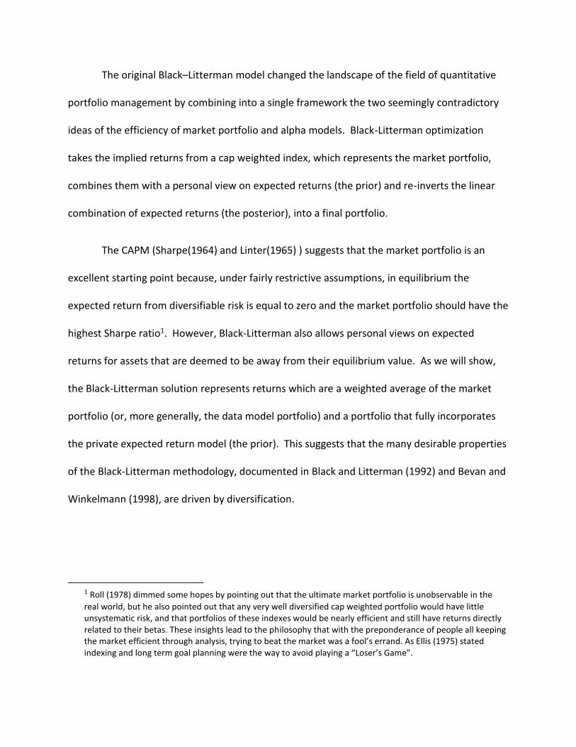
The original Black–Litterman model changed the landscape of the field of quantitative
portfolio management by combining into a single framework the two seemingly contradictory
ideas of the efficiency of market portfolio and alpha models. Black-Litterman optimization
takes the implied returns from a cap weighted index, which represents the market portfolio,
combines them with a personal view on expected returns (the prior) and re-inverts the linear
combination of expected returns (the posterior), into a final portfolio.
The CAPM (Sharpe(1964) and Linter(1965) ) suggests that the market portfolio is an
excellent starting point because, under fairly restrictive assumptions, in equilibrium the
expected return from diversifiable risk is equal to zero and the market portfolio should have the
highest Sharpe ratio1. However, Black-Litterman also allows personal views on expected
returns for assets that are deemed to be away from their equilibrium value. As we will show,
the Black-Litterman solution represents returns which are a weighted average of the market
portfolio (or, more generally, the data model portfolio) and a portfolio that fully incorporates
the private expected return model (the prior). This suggests that the many desirable properties
of the Black-Litterman methodology, documented in Black and Litterman (1992) and Bevan and
Winkelmann (1998), are driven by diversification.
1 Roll (1978) dimmed some hopes by pointing out that the ultimate market portfolio is unobservable in the
real world, but he also pointed out that any very well diversified cap weighted portfolio would have little unsystematic risk, and that portfolios of these indexes would be nearly efficient and still have returns directly related to their betas. These insights lead to the philosophy that with the preponderance of people all keeping the market efficient through analysis, trying to beat the market was a fool’s errand. As Ellis (1975) stated indexing and long term goal planning were the way to avoid playing a “Loser’s Game”.
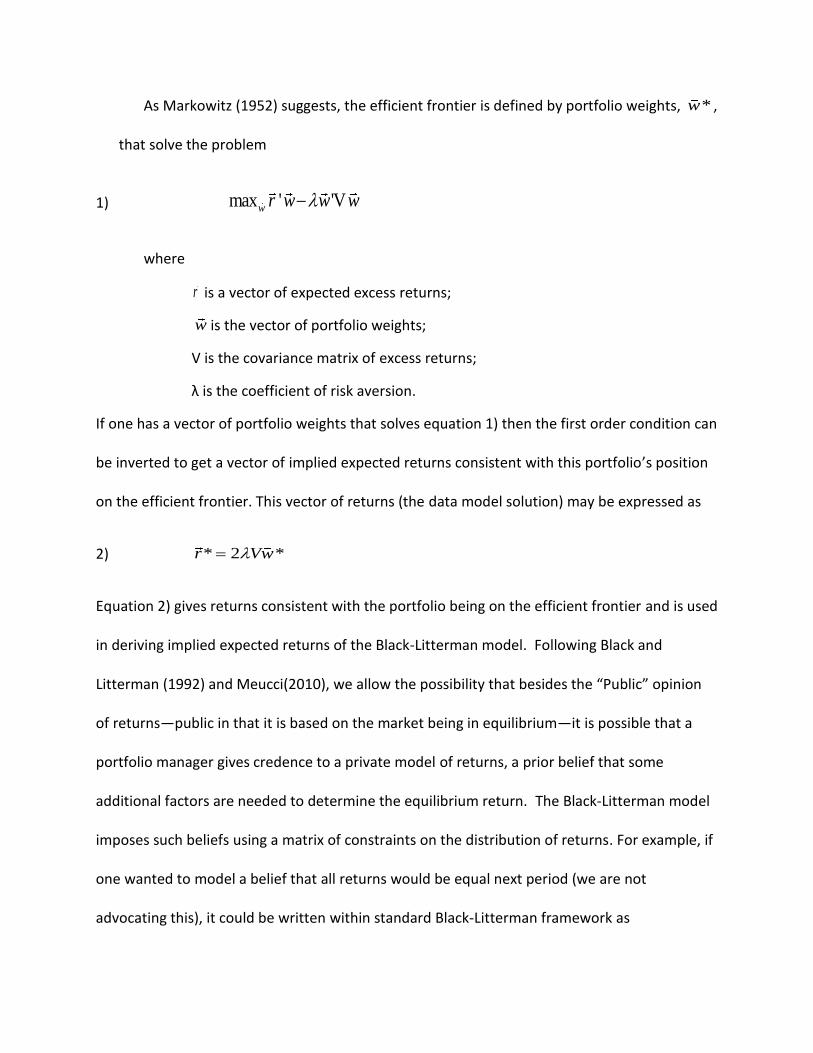
As Markowitz (1952) suggests, the efficient frontier is defined by portfolio weights, *w ,
that solve the problem
1) max ' 'Vw r w w w
where
r is a vector of expected excess returns;
w is the vector of portfolio weights;
V is the covariance matrix of excess returns;
λ is the coefficient of risk aversion.
If one has a vector of portfolio weights that solves equation 1) then the first order condition can
be inverted to get a vector of implied expected returns consistent with this portfolio’s position
on the efficient frontier. This vector of returns (the data model solution) may be expressed as
2) * 2 *r Vw
Equation 2) gives returns consistent with the portfolio being on the efficient frontier and is used
in deriving implied expected returns of the Black-Litterman model. Following Black and
Litterman (1992) and Meucci(2010), we allow the possibility that besides the “Public” opinion
of returns—public in that it is based on the market being in equilibrium—it is possible that a
portfolio manager gives credence to a private model of returns, a prior belief that some
additional factors are needed to determine the equilibrium return. The Black-Litterman model
imposes such beliefs using a matrix of constraints on the distribution of returns. For example, if
one wanted to model a belief that all returns would be equal next period (we are not
advocating this), it could be written within standard Black-Litterman framework as
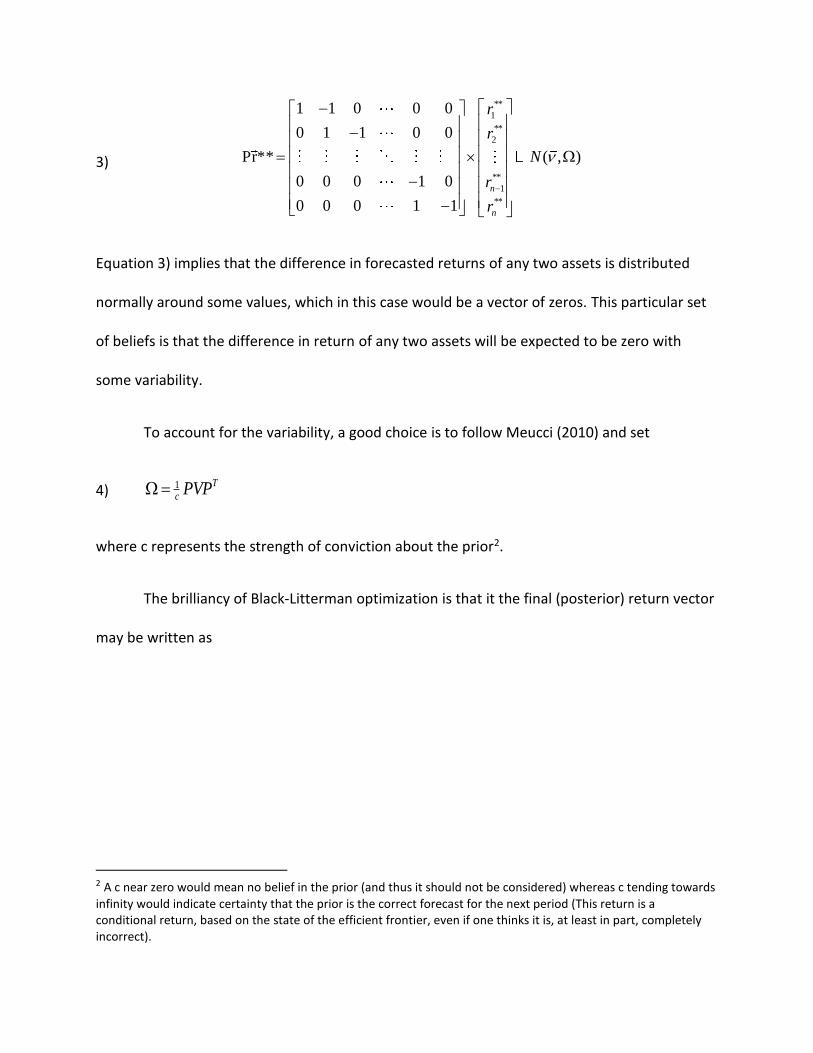
3)
**
1
**
2
**
1
**
1 1 0 0 0
0 1 1 0 0
Pr** ( , )
0 0 0 1 0
0 0 0 1 1
n
n
r
r
N
r
r
Equation 3) implies that the difference in forecasted returns of any two assets is distributed
normally around some values, which in this case would be a vector of zeros. This particular set
of beliefs is that the difference in return of any two assets will be expected to be zero with
some variability.
To account for the variability, a good choice is to follow Meucci (2010) and set
4) 1 T
cPVP
where c represents the strength of conviction about the prior2.
The brilliancy of Black-Litterman optimization is that it the final (posterior) return vector
may be written as
2 A c near zero would mean no belief in the prior (and thus it should not be considered) whereas c tending towards
infinity would indicate certainty that the prior is the correct forecast for the next period (This return is a conditional return, based on the state of the efficient frontier, even if one thinks it is, at least in part, completely incorrect).
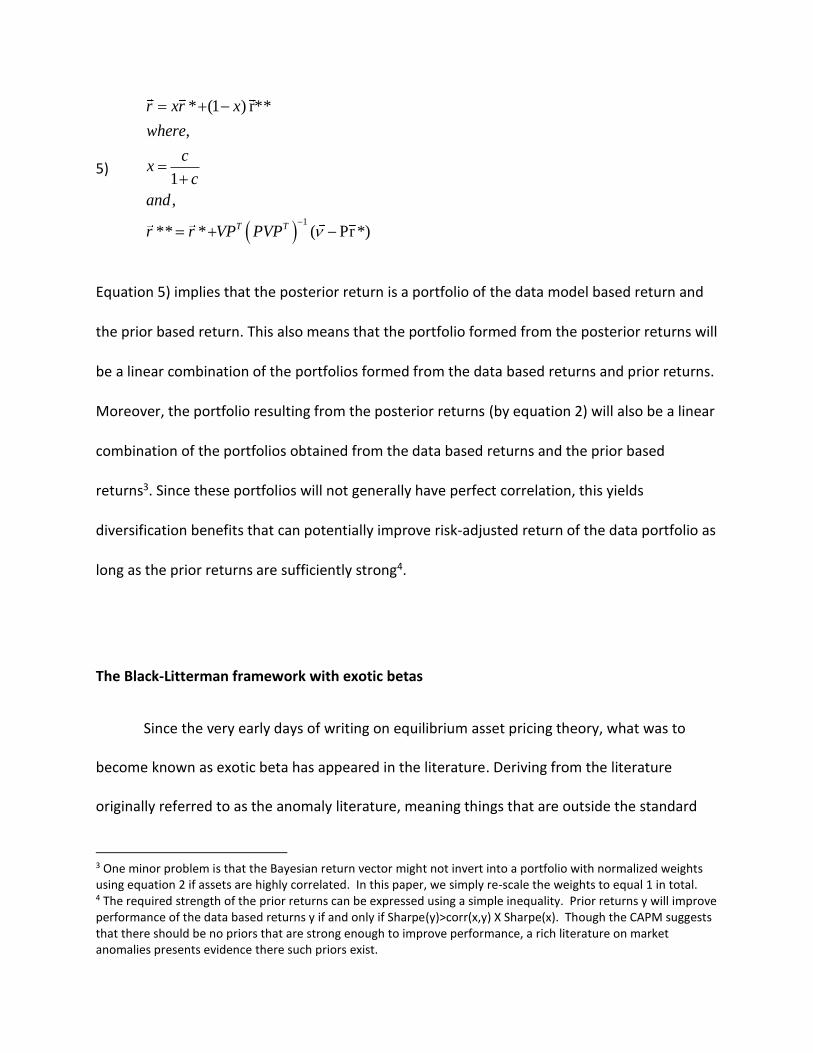
5)
1
* (1 ) r**
,
1
,
** * ( Pr *)T T
r xr x
where
cx
c
and
r r VP PVP
Equation 5) implies that the posterior return is a portfolio of the data model based return and
the prior based return. This also means that the portfolio formed from the posterior returns will
be a linear combination of the portfolios formed from the data based returns and prior returns.
Moreover, the portfolio resulting from the posterior returns (by equation 2) will also be a linear
combination of the portfolios obtained from the data based returns and the prior based
returns3. Since these portfolios will not generally have perfect correlation, this yields
diversification benefits that can potentially improve risk-adjusted return of the data portfolio as
long as the prior returns are sufficiently strong4.
The Black-Litterman framework with exotic betas
Since the very early days of writing on equilibrium asset pricing theory, what was to
become known as exotic beta has appeared in the literature. Deriving from the literature
originally referred to as the anomaly literature, meaning things that are outside the standard
3 One minor problem is that the Bayesian return vector might not invert into a portfolio with normalized weights using equation 2 if assets are highly correlated. In this paper, we simply re-scale the weights to equal 1 in total. 4 The required strength of the prior returns can be expressed using a simple inequality. Prior returns y will improve performance of the data based returns y if and only if Sharpe(y)>corr(x,y) X Sharpe(x). Though the CAPM suggests that there should be no priors that are strong enough to improve performance, a rich literature on market anomalies presents evidence there such priors exist.
canon of CAPM orthodoxy, these non-CAPM risk factors began to really take Shape with Fama
and French (1984) and later with Carhart et.al (1997). Carhart et. al. (2014) explores the notion
of exotic beta rather fully and comes to conclusions that exotic beta is a powerful portfolio
management tool. Carhart et. al (2014) define exotic betas as exposures to risk factors that are
uncorrelated with global equity markets and have positive expected returns. This definition
suggests that exotic betas are perfect candidates for prior opinions that can be effectively
incorporated within the Black-Litterman framework as long as they can be described through a
formula that is similar to equation 3).
On the one hand, exotic betas seem to invalidate the Black-Litterman framework that
assumes that market portfolio is nearly efficient. If CAPM were true, the market portfolio
would account for all systematic risk and no prior return vector (due to exotic beta, or
otherwise) would be needed. So, when one is using a Black-Litterman framework, the starting
index portfolio may be thought of as approximately on the efficient frontier but there is some
inefficiency (or weighted group of inefficiencies) that can be added to the market returns to
make more accurate asset return forecasts.
Another interpretation of this is that the Black-Litterman approach can be thought of as
a mixture model where one believes there is a 1/(1+c) chance that the market is efficient by
itself and the implied expectations are correct, and a c/(1+c) chance that a different set of
return expectations is the efficient portfolio. The mixture of the two results in hybrid forecasts
of asset returns that are part market portfolio return and an exotic beta return. Of course,
many methods of applying exotic betas are possible but the additional benefit of this method is
that it provides a distinctly different approach to extracting returns from exotic betas from the
ones documented in the literature.
<Table 1>
To make this discussion more concrete Table 1 gives descriptive of 10 DOW Jones
Industrial stocks from the period January 1995 to May 2015, whose returns are observed
monthly. The choice of ten as the number of stocks studied was to make covariance estimation
a trivial issue that would not interfere with the main points of the paper.5
We illustrate how to incorporate exotic betas in the Black-Litterman framework by
starting with a capitalization weighted portfolio of the ten stocks and using the low volatility
anomaly, described in Jagannathan and Ma (2003), as an example of an exotic beta. In this case
the future expected Sharpe ratio is considered to be an inverse function of previous volatility.
An easy way to represent this prior within the current framework is to say that for any pair of
assets, the expected difference in their Sharpe ratios going forward, is a percent of the trailing
difference in their inverse volatility.
Specifically, this prior return, consistent with the low volatility anomaly, may be written
for all assets as
5 There is no consensus as to the optimal estimation method for larger covariance matrices, but a number of approaches have been introduced. Wolf and Ledoit (2004) suggest shrinking a sample covariance matrix, Jagannathan and Ma (2003) consider using daily returns and factor models in addition to shrinkage, Pafka, Potters and Kondor (2004) argue for applying filtering based on the random matrix theory. The issue of estimating covariance matrix is outside of the scope of this paper. For this particular small problem covariance estimates relay on a simple 60 month sample.
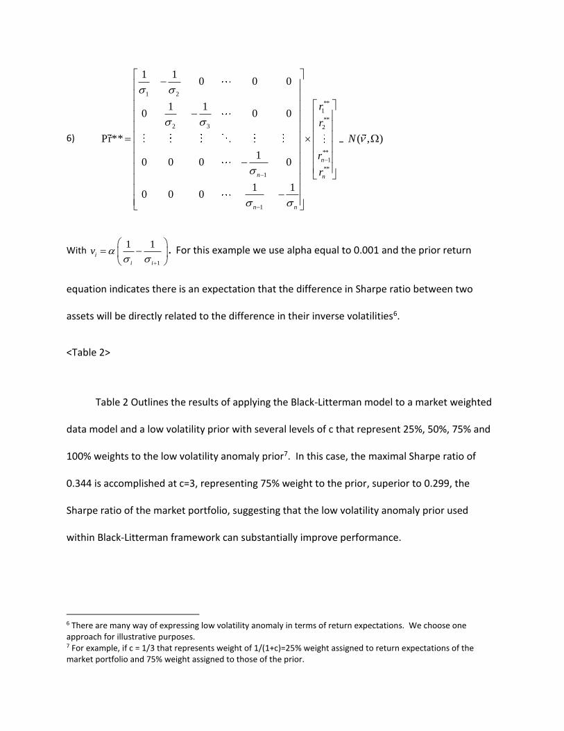
6)
1 2
**
1
**2 3 2
**
1
**1
1
1 10 0 0
1 10 0 0
Pr** ( , )
10 0 0 0
1 10 0 0
n
n n
n n
r
r
N
r
r
With 1
1 1i
i i
v
. For this example we use alpha equal to 0.001 and the prior return
equation indicates there is an expectation that the difference in Sharpe ratio between two
assets will be directly related to the difference in their inverse volatilities6.
<Table 2>
Table 2 Outlines the results of applying the Black-Litterman model to a market weighted
data model and a low volatility prior with several levels of c that represent 25%, 50%, 75% and
100% weights to the low volatility anomaly prior7. In this case, the maximal Sharpe ratio of
0.344 is accomplished at c=3, representing 75% weight to the prior, superior to 0.299, the
Sharpe ratio of the market portfolio, suggesting that the low volatility anomaly prior used
within Black-Litterman framework can substantially improve performance.
6 There are many way of expressing low volatility anomaly in terms of return expectations. We choose one approach for illustrative purposes. 7 For example, if c = 1/3 that represents weight of 1/(1+c)=25% weight assigned to return expectations of the market portfolio and 75% weight assigned to those of the prior.
Another interesting result is posed by the experiment in Table 3. Table 3 compares
performance of the standard implementation of the low volatility anomaly and our
implementation that is based on the Black-Litterman framework. The standard implementation
ranks stocks based on their in-sample volatility and then buys the bottom quintile of stocks
(low-volatility stocks) and sells short the top quintile of stocks (high-volatility stocks). Portfolio
weights are inversely proportional to historical inverse volatilities. The Bayesian prior approach
purchases the Black-Litterman portfolio with c=∞ (100% weight to the low volatility anomaly
prior) and sells short the market portfolio. The Bayesian prior approach measures the
incremental benefit of utilizing the low volatility prior within Black-Litterman framework.
<Table 3>
The Sharpe ratio of the Bayesian prior approach is equal to 0.14 which is more than twice
0.06, the Sharpe ratio of the standard implementation of the low volatility anomaly. Though
the relative performance of the two implementations of low volatility anomaly (or any exotic
beta in general) can be sensitive to the time period, portfolio constituents and choice of
parameters, the Bayesian prior approach substantially expands the toolbox of exotic beta
strategies with potentially significant performance implications for investors.
Carhart et al (2014) suggest that utilizing a limited version of Black-Litterman with exotic
betas as portfolio constituents is unlikely to diminish its power. We have extended this result
by showing that the standard Black-Litterman implementation can be combined with exotic
betas by using them as priors, achieving multiple useful results. In the next sections we
challenge the assumption of market efficiency and using market as the starting point in the
Black-Litterman portfolio. Though the topic of market efficiency has been discussed in the
literature, this paper is the first one to investigate its implications for Black-Litterman
optimization and suggest a version of Black-Litterman optimization that extends its application
to many new investment situations.
The Market Portfolio, the Risk Parity Portfolio, and Efficiency
While the CAPM suggests that a capitalization-weighted market portfolio should have
the highest Sharpe ratio, there are situations in which the market portfolio is either suboptimal,
or even inappropriate. For example, fund of hedge funds allocation decisions, and decisions
involving futures contracts generally, do not readily admit capitalization calculations which
makes capitalization-weighted market portfolio unattainable. Moreover, Asness et al (2012)
suggests that the market portfolio is not efficient and instead argue that the risk parity portfolio
approach which equalizes contribution to portfolio risk from each constituent is more efficient
due to leverage aversion8. Qian (2006) provides a comprehensive analysis of risk-parity
portfolios. Also, we have outlined the technical details of the risk parity approach in the
Appendix.
8 The authors argue that leverage aversion changes the predictions of modern portfolio theory because investors without access to leverage are unable to benefit from higher risk-adjusted returns of safer (low beta or low volatility) assets. Risk parity portfolios overweight safer assets relative to the market portfolio and benefit from their higher risk-adjusted returns after applying leverage.
Since capitalization weights are available in the 10 stock Dow Jones example, we can
easily compare performance of the capitalization-weighted market portfolio and Risk Parity.
Table 4 reports out-of-sample performance of the two portfolios.
<Table 4>
The Risk Parity portfolio delivers Sharpe ratio of 0.45 which is higher than 0.30, the
Sharpe ratio of the market portfolio. We need to be careful about drawing conclusions about
efficiency of risk parity from this simple example. Anderson et al (2012) argue that empirical
studies that make claims about the efficiency of risk parity might be very sensitive to the time
period studied and the transaction costs assumed. Our simple example also is not immune to
their criticism.
To summarize, there is reason to believe that at least sometimes an equal risk weighted
index portfolio may be more efficient than a capitalization weighted portfolio. Also, there are
times when capitalization weights are unavailable. In either of these situations the risk parity
portfolio makes a good candidate for the data based starting point in the Black-Litterman
framework9.
Bayesian Risk Parity
9 Although some people may find the notion that the equal risk portfolio is possibly efficient to be strange, even less likely diversified portfolios have been shown to be efficient in some cases. DeMiguel et al. (2009) maintain that for their universe the equal weighted (1/N) portfolio was more efficient than more conventional alternatives.
The importance of the Black-Litterman framework is that it provides a way of mixing
market data based returns with prior beliefs about returns that are not priced properly by the
market. A key thing to realize is that reversing the first order condition in the Markowitz model
is theoretically permissible to any portfolio on the efficient frontier. That is, the efficient
frontier is defined by the solution to equation 1) and efficient portfolios are given as the
solutions of the first order condition by equation 2) with the choice of lambda determining the
exact portfolio. And, as previously noted, the exact lambda chosen, and thus exactly which
efficient portfolio is used, is not important to the Black-Litterman solution. However, it is
important to note that the use of the capitalization weighted portfolio as the starting point is
based on a theoretical assumption, not a mathematical necessity. It is an assumption that the
market is an efficient portfolio, and may therefore be used, or that the capitalization weighted
portfolio may be used in the case of a market subset optimization.
Having established in the previous section that the risk parity can be considered a
reasonable efficient portfolio, it can be used as a starting point for Black-Litterman optimization
in calculation of implied expected returns. One interesting thing brought out in the Appendix is
that the risk parity portfolio simply says that each assets contribution to total risk should be
made equal. This does not mean that each asset should have the same Sharpe ratio or same
expected return. Therefore, provided one believes that the risk parity portfolio is efficient (at
least approximately) there is no logical problem with using it as a starting point10 to obtain a
10 The starting point of the Black-Litterman portfolio can be any index portfolio that is efficient. Both market and risk parity portfolio are indices. Market portfolio is capitalization-weighted and risk parity is risk-weighted.
vector of data model returns11 with the same benefit of utilizing priors based on exotic betas12.
We define Bayesian Risk Parity as the generalized version of Black-Litterman optimization that
uses risk parity as the starting point and exotic betas as priors.
Two Examples of Bayesian Risk Parity
We illustrate the Bayesian Risk Parity approach by considering two simple examples
with investments in three major asset classes—stocks, bonds, and commodities. The data for
these experiments covers the period from March 1976 through May 2015, and consists of the
MSCI World Index as a proxy for the stock market, the Barclay US Aggregate Government Index
to represents the bond market, and the S&P Goldman Sachs Commodity Index to represents
commodities. We use the three-month Treasury bill secondary market rate as proxy of the risk
free rate. Inclusion of commodities is particularly interesting because they don’t have
capitalization weights and, therefore, capitalization-weighted market portfolio is
unattainable13.
Table 5 presents some relevant descriptive statistics of the data. One interesting
statistic is that over this time period the three asset classes have performed very differently
11 Moreover, a fund of hedge fund manager that believes that the hedge funds in the portfolio have approximately the same risk-adjusted return can improve upon risk-parity approach by imposing that belief within Bayesian Risk Parity approach. 12 The same example of 10 DJ stocks with low volatility anomaly but with risk parity used as the original portfolio, we observe an improvement of Sharpe over the classic risk parity but that improvement is not as substantial as in the case of market portfolio. 13 Portfolio allocations that involve hedge funds are another example of limitation of capitalization-weighted approach.
with commodities performing worst with the Sharpe ratio of -0.04 and bonds performing best
with the Sharpe ratio of 0.51.
<Table 5>
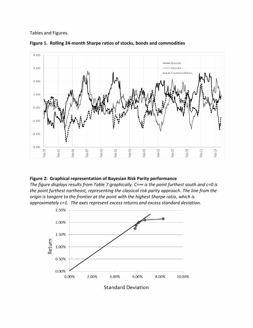
However, the relative performance of the three asset classes is very inconsistent across
time. Figure 1 displays rolling 24 month Sharpe of the three assets.14
<Figure 1>
Absolute and relative performance is inconsistent across time with the range of Sharpe ratios
between around -2.5 and almost 3.
The first step of Bayesian Risk Parity is calculating risk parity weights and corresponding
implied expected excess returns using equation 2. The second steps involves imposing beliefs.
We consider two examples that can have broad applications to many investors. The first
example considers momentum as an exotic beta that is robust across most asset classes as
documented in Asness et al (2013). The second example considers an equal Sharpe ratio prior.
Bayesian Risk Parity with Momentum
Momentum is a pervasive anomaly that has been extensively documented in the
literature. We express belief in momentum in Sharpe ratios using equation 6 with the same
14 For this section we choose to use a rolling 24 month’s sample estimates for all covariance and variance estimates. With only three assets, a longer period is not required.
matrix P and vector 1
1
i ii
i i
R Rv
. We set alpha equal to .05 which represents the belief
that the difference in future Sharpe ratios of any two assets is expected to equal 5% of the most
recent Sharpe ratios. In this simple example we use a time window of 24 months to estimate
recent Sharpe ratios. As before, we use the same levels of c that represent 25%, 50%, 75% and
100% weights to the exotic beta belief. The results of this experiment are presented in Table 6.
<Table 6>
In this case, the maximal Sharpe ratio of 0.35 occurs at c=3, representing 75% weight to
the prior, superior to 0.253, the Sharpe ratio of the risk-parity portfolio, suggesting that the
momentum in risk-adjusted return prior used within Black-Litterman framework can improve
performance.
Bayesian Risk Parity with equal Sharpe
Though belief in equal Sharpe ratios is unrelated to exotic beta, it is also an interesting
case to study. There is a sizable group of investors who hold that belief about diversified asset
classes. Also there are fund of (hedge) funds managers who impose very high requirements for
their hedge funds, reflected in rigorous due diligence steps, resulting in approximately the same
Sharpe expectations across hedge funds in the portfolio. Finally, it is illustrative to show how
even a fairly weak prior performs in the Black-Litterman framework.
Table 5 shows that commodities have substantially underperformed stocks and bonds
over the time period of this study. However, other studies such as Gorton and Rouwenhorst
(2006) argue that an equally-weighted index of commodity futures monthly returns should
deliver Sharpe ratio comparable to that of equities. The equal Sharpe belief can be expressed
using equation 6) with the mean vector set to zero.
<Table 7>
Table 7 reports results of the out-of-sample performance. The maximal Sharpe ratio of
0.316 is corresponds to c=1, representing 50% weight to the prior, superior to 0.253, the Sharpe
ratio of the risk-parity portfolio. This suggests that the prior of equal Sharpe used within Black-
Litterman framework can add value.
The Bayesian approach allows for combinations of data and prior that reach Sharpe
ratios not obtainable through either approach alone. The exact nature of this improvement is
apparent in Figure 2. Figure 2 presents the data of Table 7 in graphical form, and once again
demonstrates the diversifying power of Black-Litterman even in the face of a rather weak prior.
<Figure 2>
The curve, reminiscent of a Markowitz frontier, reiterates the benefits of diversification
produced by the Bayesian Risk Parity method. The straight line from the origin to the
combination line of strategic outcomes shows that the maximum obtainable Sharpe ratio is at
approximately c=1 for this particular combination of strategies and assets over this particular
period. While it is true that this diversification benefit would occur with almost any prior, there
are of, of course, better opportunities the better the prior actually is.
Conclusion
In this paper we demonstrate that using exotic beta as a prior alpha model in the
Black-Litterman optimization is attractive to investors who already utilize the classic Black-
Litterman approach and seek to incorporate advances in the exotic beta research, and those
who focus on practical implementation of exotic betas. The reason for this behavior is the
diversification of alpha sources benefits an investor, whether he or she wishes a portfolio that is
mainly efficient portfolio based, mainly exotic beta based, or the one that maximizes Sharpe
ratio.
Additionally, we introduce Bayesian Risk Parity, an extension to the Black–Litterman
model that incorporates exotic betas as substitutes to scarce and costly expert opinions and
relaxes the assumption of market efficiency by utilizing risk parity that does not rely on
capitalization weights and tends to be more efficient than the market portfolio. The framework
captures the power of Black-Litterman optimization in situations when capitalization weights
are unavailable as in the case of hedge funds and commodities. The methodology leverages
advances in exotic beta research without having to replicate exotic beta portfolios directly.
Bayesian Risk Parity symbiotically unifies the Black–Litterman optimization, exotic betas, and
risk parity into a single flexible framework that combines the various strengths of the three
approaches to improve investors’ portfolios. These results allow a large number of investment
professionals to place new tools into their investment tool box, without throwing out
everything they might have been previously using.
Appendix
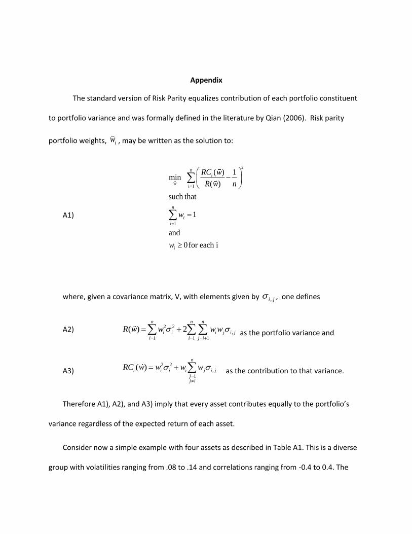
The standard version of Risk Parity equalizes contribution of each portfolio constituent
to portfolio variance and was formally defined in the literature by Qian (2006). Risk parity
portfolio weights, iw , may be written as the solution to:
A1)
2n
wi 1
1
( ) 1min
( )
such that
1
and
0for each i
i
n
i
i
i
RC w
R w n
w
w
where, given a covariance matrix, V, with elements given by ,i j , one defines
A2) 2 2
,
1 1 1
( ) 2n n n
i i i j i j
i i j i
R w w w w
as the portfolio variance and
A3) 2 2
,
1
( )n
i i i i j i j
jj i
RC w w w w
as the contribution to that variance.
Therefore A1), A2), and A3) imply that every asset contributes equally to the portfolio’s
variance regardless of the expected return of each asset.
Consider now a simple example with four assets as described in Table A1. This is a diverse
group with volatilities ranging from .08 to .14 and correlations ranging from -0.4 to 0.4. The
weights given range from a low or 15.3% for asset A to 28.5% percent for asset C. The weights
sum to 100% and the assets each contributes 25% to the total volatility as defined in equations
A1), A2), and A3).
<Table A1>
Continuing with the assets from Table A1, and assuming the risk aversion parameter, λ,
equals one, Table A2 gives implied expectations for the four assets described above. It is useful
to note that by the reverse optimization measure risk parity does not assume equal risk-
adjusted returns among assets, as is a popular misconception among some practitioners. In
this case, the ratio of the implied Sharpe of asset A is about 1.6 times bigger than that of asset
C.
<Table A2>
References
Anderson, Robert, Stephen Bianchi, and Lisa Goldberg. 2012. “Will My Risk Parity Strategy Outperform?” Financial Analysts Journal 68, 75-93.
Asness, Clifford, Andrea Frazzini, and Lasse Pedersen. 2012. “Leverage Aversion and Risk Parity.” Financial Analysts Journal 68, 47-59.
Asness, Clifford, Tobias Moskowitz, and Lasse Pedersen. 2013. “Value and Momentum Everywhere.” Journal of Finance 68, 929-985.
Black, Fischer, and Robert Litterman. 1992. “Global portfolio optimization”, Financial Analysts Journal 48, 28-43.
Beven, Andrew, and Kurt Winkelmann. 2004. “Using the Black-Litterman Global Asset Allocation Model: Three Years of Practical Experience. ” Goldman Sachs white paper.
Carhart, Mark, Ul-Wing Cheah, Giorgio De Santis, Harry Farrell, and Robert Litterman. 2014. “Exotic Betas Revisited. ” Financial Analysts Journal 70, 24-52.
DiMiguel, Victor, Lorenzo Garlappi, and Raman Uppal. 2009. “Optimal Versus Naïve Diversification: How Inefficient is the 1/N Portfolio Strategy.” Review of Financial Studies 22, 1915-1953.
Ellis, Charles. 1975. “The Loser’s Game.” Financial Analysts Journal 31(4), 19-26.
Gorton, Gary, and K. Gert Rouwenhorst. 2006. “Facts and Fantasies about Commodity Futures.” Financial Analysts Journal 62, 47-68.
Jagannathan, Ravi, and Tongshu Ma. 2004. “Risk Reduction in Large Portfolios: Why Imposing the Wrong Constraints help.” Journal of Finance 58, 1651-1684.
Ledoit, Olivier, and Michael Wolf. 2004. “Honey, I Shrunk the Sample Covariance Matrix.” Journal of Portfolio Management 30, 110-119. Markowitz, Harry. 1952. “Portfolio Selection.” Journal of Finance 7, 77-91.
Meucci, Attilio. 2010. “The Black-Litterman Approach: Original Model and Extensions.” The Encyclopedia of Quantitative Finance (R. Cont, editor), 196-199, Wiley, New York.
Pafka, Szilard, Marc Potters, and Imre Kondor. 2004. “Exponential weighting and random-matrix-theory-based filtering of financial covariance matrices for portfolio optimization.” available at http://arxiv.org/pdf/cond-mat/0402573.pdf.
Roll, Richard. 1978. “Ambiguity When Performance is Measured by the Securities Market Line.” Journal of Finance 33, 1051-1069.

Qian, Edward. 2006. “On the financial interpretation of risk contribution: risk budgets do add up.” Journal of Investment Management 4, 41-51.
Yang, Zhongjin, Keli Han, Marat Molyboga, and Georgiy Molyboga. 2015. “A simple approach to evaluating the stability of optimal portfolios.” Journal of Investing (forthcoming).
Tables and Figures.
Figure 1. Rolling 24-month Sharpe ratios of stocks, bonds and commodities
Figure 2: Graphical representation of Bayesian Risk Parity performance The figure displays results from Table 7 graphically. C=∞ is the point furthest south and c=0 is the point furthest northeast, representing the classical risk parity approach. The line from the origin is tangent to the frontier at the point with the highest Sharpe ratio, which is approximately c=1. The axes represent excess returns and excess standard deviation.
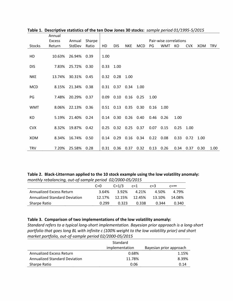
Table 1. Descriptive statistics of the ten Dow Jones 30 stocks: sample period 01/1995-5/2015
Annual Excess Annual Sharpe Pair-wise correlations
Stocks Return StdDev Ratio HD DIS NKE MCD PG WMT KO CVX XOM TRV
HD 10.63% 26.94% 0.39
1.00
DIS 7.83% 25.72% 0.30
0.33
1.00
NKE 13.74% 30.31% 0.45
0.32
0.28
1.00
MCD 8.15% 21.34% 0.38
0.31
0.37
0.34
1.00
PG 7.48% 20.29% 0.37
0.09
0.10
0.16
0.25
1.00
WMT 8.06% 22.13% 0.36
0.51
0.13
0.35
0.30
0.16
1.00
KO 5.19% 21.40% 0.24
0.14
0.30
0.26
0.40
0.46
0.26
1.00
CVX 8.32% 19.87% 0.42
0.25
0.32
0.25
0.37
0.07
0.15
0.25
1.00
XOM 8.34% 16.74% 0.50
0.14
0.29
0.16
0.34
0.22
0.08
0.33
0.72
1.00
TRV 7.20% 25.58% 0.28
0.31
0.36
0.37
0.32
0.13
0.26
0.34
0.37
0.30
1.00
Table 2. Black-Litterman applied to the 10 stock example using the low volatility anomaly: monthly rebalancing, out-of-sample period 02/2000-05/2015
C=0 C=1/3 c=1 c=3 c=∞
Annualized Excess Return 3.64% 3.92% 4.21% 4.50% 4.79%
Annualized Standard Deviation 12.17% 12.15% 12.45% 13.10% 14.08%
Sharpe Ratio 0.299 0.323 0.338 0.344 0.340
Table 3. Comparison of two implementations of the low volatility anomaly: Standard refers to a typical long-short implementation. Bayesian prior approach is a long-short portfolio that goes long BL with infinite c (100% weight to the low volatility prior) and short market portfolio, out-of-sample period 02/2000-05/2015
Standard implementation Bayesian prior approach
Annualized Excess Return 0.68% 1.15%
Annualized Standard Deviation 11.78% 8.39%
Sharpe Ratio 0.06 0.14
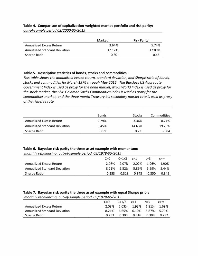
Table 4. Comparison of capitalization-weighted market portfolio and risk parity: out-of-sample period 02/2000-05/2015
Market Risk Parity
Annualized Excess Return 3.64% 5.74%
Annualized Standard Deviation 12.17% 12.89%
Sharpe Ratio 0.30 0.45
Table 5. Descriptive statistics of bonds, stocks and commodities. This table shows the annualized excess return, standard deviation, and Sharpe ratio of bonds, stocks and commodities for March 1976 through May 2015. The Barclays US Aggregate Government Index is used as proxy for the bond market, MSCI World Index is used as proxy for the stock market, the S&P Goldman Sachs Commodities Index is used as proxy for the commodities market, and the three month Treasury bill secondary market rate is used as proxy of the risk-free rate.
Bonds Stocks Commodities
Annualized Excess Return 2.79% 3.36% -0.71%
Annualized Standard Deviation 5.45% 14.63% 19.26%
Sharpe Ratio 0.51 0.23 -0.04
Table 6. Bayesian risk parity the three asset example with momentum: monthly rebalancing, out-of-sample period 03/1978-05/2015
C=0 C=1/3 c=1 c=3 c=∞
Annualized Excess Return 2.08% 2.07% 2.02% 1.96% 1.90%
Annualized Standard Deviation 8.21% 6.52% 5.89% 5.59% 5.44%
Sharpe Ratio 0.253 0.318 0.343 0.350 0.349
Table 7. Bayesian risk parity the three asset example with equal Sharpe prior: monthly rebalancing, out-of-sample period 03/1978-05/2015
C=0 C=1/3 c=1 c=3 c=∞
Annualized Excess Return 2.08% 2.03% 1.93% 1.81% 1.69% Annualized Standard Deviation 8.21% 6.65% 6.10% 5.87% 5.79% Sharpe Ratio 0.253 0.305 0.316 0.308 0.292
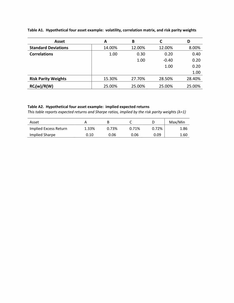
Table A1. Hypothetical four asset example: volatility, correlation matrix, and risk parity weights
Asset A B C D
Standard Deviations 14.00% 12.00% 12.00% 8.00%
Correlations 1.00 0.30 0.20 0.40
1.00 -0.40 0.20
1.00 0.20
1.00
Risk Parity Weights 15.30% 27.70% 28.50% 28.40%
RCi(w)/R(W) 25.00% 25.00% 25.00% 25.00%
Table A2. Hypothetical four asset example: implied expected returns This table reports expected returns and Sharpe ratios, implied by the risk parity weights (λ=1)
Asset A B C D Max/Min
Implied Excess Return 1.33% 0.73% 0.71% 0.72% 1.86
Implied Sharpe 0.10 0.06 0.06 0.09 1.60