blackmax final
TRANSCRIPT

8/3/2019 BlackMax Final
http://slidepdf.com/reader/full/blackmax-final 1/29
BlackMax: A black-hole event generator with rotation, recoil, split branes, and brane tension
De-Chang Dai,1 Glenn Starkman,1 Dejan Stojkovic,2 Cigdem Issever,3 Eram Rizvi,4 and Jeff Tseng3
1Case Western Reserve University, Cleveland, Ohio 44106-7079, USA2 Department of Physics, SUNY at Buffalo, Buffalo, New York 14260-1500, USA
3University of Oxford, Oxford, United Kingdom4Queen Mary, University of London, London, United Kingdom
(Received 26 November 2007; published 15 April 2008)
We present a comprehensive black-hole event generator, BlackMax, which simulates the experimentalsignatures of microscopic and Planckian black-hole production and evolution at the LHC in the context of
brane world models with low-scale quantum gravity. The generator is based on phenomenologically
realistic models free of serious problems that plague low-scale gravity, thus offering more realistic
predictions for hadron-hadron colliders. The generator includes all of the black-hole gray-body factors
known to date and incorporates the effects of black-hole rotation, splitting between the fermions, nonzero
brane tension, and black-hole recoil due to Hawking radiation (although not all simultaneously). The
generator can be interfaced with HERWIG and PYTHIA. The main code can be downloaded from http://
www-pnp.physics.ox.ac.uk/~issever/BlackMax/blackmax.html.
DOI: 10.1103/PhysRevD.77.076007 PACS numbers: 04.50.Gh, 04.70.Dy
I. INTRODUCTIONModels with TeV-scale quantum gravity [1–4] offer very
rich collider phenomenology. Most of them assume the
existence of a three-plus-one-dimensional hypersurface,
which is referred as ‘‘the brane,’’ where standard model
particles are confined, while only gravity and possibly
other particles that carry no gauge quantum numbers,
such as right-handed neutrinos can propagate in the full
space, the so-called ‘‘bulk.’’ Under certain assumptions,
this setup allows the fundamental quantum-gravity energy
scale, M , to be close to the electroweak scale. The ob-
served weakness of gravity compared to other forces on the
brane (i.e. in the laboratory) is a consequence of the large
volume of the bulk which dilutes the strength of gravity.In the context of these models of TeV-scale quantum
gravity, probably the most exciting new physics is the
production of micro-black-holes in near-future accelera-
tors like the Large Hadron Collider (LHC) [5]. According
to the ‘‘hoop conjecture’’ [6], if the impact parameter of
two colliding particles is less than 2 times the gravitational
radius, rh, corresponding to their center-of-mass energy
(ECM), a black hole with a mass of the order of ECM and
horizon radius, rh, will form. Typically, this gravitational
radius is approximately ECM=M 2. Thus, when particles
collide at center-of-mass energies above M , the probabil-
ity of black-hole formation is high.
Strictly speaking, there exists no complete calculation
(including radiation during the process of formation and
backreaction) which proves that a black hole really forms.
It may happen that a true event horizon and singularity
never forms, and that Hawking (or rather Hawking-like)
radiation is never quite thermal. In [7], this question was
analyzed in detail from a point of view of an asymptotic
observer, who is in the context of the LHC the most
relevant observer. It was shown that, though such observers
never observe the formation of an event horizon even in the
full quantum treatment, they do register pre-Hawkingquantum radiation that takes away energy from a collaps-
ing system. Pre-Hawking radiation is nonthermal and be-
comes thermal only in the limit when the horizon is
formed. Since a collapsing system has only a finite amount
of energy, it disappears before the horizon is seen to be
formed. While these results have important implications
for theoretical issues like the information loss paradox, in a
practical sense very little will change. The characteristic
time for gravitational collapse in the context of collisions
of particles at the LHC is very short. This implies that pre-
Hawking radiation will be quickly experimentally indis-
tinguishable from Hawking radiation calculated for a real
black hole. Also, calculations in [7] indicate that the char-acteristic time in which a collapsing system loses all of its
energy is very similar to a lifetime of a real black hole.
Thus, one may proceed with a standard theory of black
holes.
Once a black hole is formed, it is believed to decay via
Hawking radiation. This Hawking radiation will consist of
two parts: radiation of standard model particles into the
brane and radiation of gravitons and any other bulk modes
into the bulk. The relative probability for the emission of
each particle type is given by the gray-body factor for that
mode. This gray-body factor depends on the properties of
the particle (charge, spin, mass, momentum), of the black
hole (mass, spin, charge) and, in the context of TeV-scale
quantum gravity, on environmental properties—the num-
ber of extra dimensions, the location of the black hole
relative to the brane (or branes), etc. In order to properly
describe the experimental signatures of black-hole produc-
tion and decay, one must therefore calculate the gray-body
factors for all of the relevant degrees of freedom.
There are several black-hole event generators available
in the literature [8] based on particular, simplified models
PHYSICAL REVIEW D 77, 076007 (2008)
1550-7998=2008=77(7)=076007(29) 076007-1 © 2008 The American Physical Society

8/3/2019 BlackMax Final
http://slidepdf.com/reader/full/blackmax-final 2/29
of low-scale quantum gravity and incorporating limited
aspects of micro-black-hole physics. Unfortunately, low-
scale gravity is plagued with many phenomenological
challenges like fast proton decay, large n n oscillations,
flavor-changing neutral currents, and large mixing between
leptons [9,10]. For a realistic understanding of the experi-
mental signature of black-hole production and decay, one
needs calculations based on phenomenologically viable
gravity models, and incorporating all necessary aspectsof the production and evolution of the black holes.
One low-scale gravity model in which the above-
mentioned phenomenological challenges can be addressed
is the split-fermion model [11]. In this model, the standard
model fields are confined to a ‘‘thick brane,’’ much thicker
than M ÿ1 . Within this thick brane, quarks and leptons are
stuck on different three-dimensional slices (or on different
branes), which are separated by much more than M ÿ1 . This
separation causes an exponential suppression of all direct
couplings between quarks and leptons, because of expo-
nentially small overlaps between their wave functions. The
proton decay rate will be safely suppressed if the spatial
separation between quarks and leptons is greater by a
factor of at least 10 than the widths of their wave functions.
Since B � 2 processes, like n n oscillations, are mediated
by operators of the type uddudd, suppressing them re-
quires a further splitting between up-type and down-type
quarks. Since the experimental limits on B � 2 operators
are much less stringent than those on B � 1 operators,
the u- and d-type quarks need only be separated by a few
times the width of their wave functions [11].
Current black-hole generators assume that the black
holes that are formed are Schwarzschild-like. However,
most of the black holes that would be formed at the LHC
would be highly rotating, due to the nonzero impact pa-rameter of the colliding partons. Because of the existence
of an ergosphere (a region between the infinite redshift
surface and the event horizon), a rotating black hole ex-
hibits superradiance: some modes of radiation get ampli-
fied compared to others. The effect of superradiance [12] is
strongly spin dependent, with emission of higher-spin
particles strongly favored. In particular, the emission of
gravitons is enhanced over lower-spin standard model
particles. Since graviton emission appears in detectors as
missing energy, the effects of black-hole rotation cannot be
ignored. Similarly, black holes may be formed with non-
zero gauge charge, or acquire charge during their decay.
This again may alter the decay properties of the black holeand should be included.
Another effect neglected in other generators is the recoil
of the black hole. A small black hole attached to a brane in
a higher-dimensional space emitting quanta into the bulk
could leave the brane as a result of a recoil.1 In this case,
visible black-hole radiation would cease. Alternately, in a
split-brane model, as a black hole traverses the thick brane
the standard model particles that it is able to emit will
change depending on which fermionic branes are nearby.
It is also the case that virtually all the work in this field
has been done for the idealized case where the brane
tension is negligible. However, one generically expects
the brane tension to be of the order of the fundamental
energy scale, being determined by the vacuum energycontributions of brane-localized matter fields [13]. As
shown in [14], finite brane tension modifies the standard
gray-body factors.
Finally, it has been suggested [15] that more common
than the formation and evaporation of black holes will be
gravitational scattering of parton pairs into a two-body
final state. We include this possibility.
Here we present a comprehensive black-hole event gen-
erator, BlackMax, that takes into account practically all of
the above-mentioned issues (although not necessarily si-multaneously), and includes almost all the necessary gray-
body factors.2 Preliminary studies show how the signatures
of black-hole production and decay change when oneincludes splitting between the fermions, black-hole rota-
tion, positive brane tension, and black-hole recoil. Future
papers will explore the implications of these changes in
greater detail.
In Sec. II and III we discuss the production of black
holes and the gray-body factors, respectively. The evapo-
ration process and final burst of the black holes is discussed
in Sec. IV and V. Sections VI and describe the input and
output of the generator. Section VII shows some character-
istic distributions of black holes for different extra-
dimension scenarios. The reference list is extensive, re-
flecting the great interest in the topic [5,6,8–10,13–104],
but by no means complete.
II. BLACK-HOLE PRODUCTION
We assume that the fundamental quantum-gravity en-
ergy scale M is not too far above the electroweak scale.
Consider two particles colliding with a center-of-mass
energy ECM. They will also have an angular momentum
J in their center-of-mass (CM) frame. By the hoop con-
jecture, if the impact parameter, b, between the two collid-
ing particles is smaller than the diameter of the horizon of a
(d� 1)-dimensional black hole (where d is the total num-ber of spacelike dimensions) of mass M
�ECM and angu-
lar momentum J ,
b < 2rh�d;M;J � ; (1)
then a black hole with rh will form. The cross section for
this process is approximately equal to the interaction area
�2rh�2.
1If the black hole carries gauge charge, it will be prevented
from leaving the brane.
2The calculation of the graviton gray-body factor for a rotating
black hole has not been achieved.
DE-CHANG DAI et al. PHYSICAL REVIEW D 77, 076007 (2008)
076007-2
8/3/2019 BlackMax Final
http://slidepdf.com/reader/full/blackmax-final 3/29
In Boyer-Lindquist coordinates, the metric for a (d� 1)-
dimensional rotating black hole (with angular momentum
parallel to the !̂ in the rest frame of the black hole) is
ds2 �
1 ÿ r4ÿd
�r; �dt2
ÿ sin2
r2 � a2
�sin2
r4ÿd
�r;
�d2
� 2asin2r4ÿd
�r; � dtdÿ �r; �
dr2
ÿ �r; �d2 ÿ r2cos2ddÿ3 ; (2)
where is a parameter related to mass of the black hole,
while
� r2 � a2cos2 (3)
and
� r2 � a2 ÿr4ÿd: (4)
The mass of the black hole is
M � �dÿ 1� Adÿ1
16Gd
; (5)
and
J � 2Ma
dÿ 1(6)
is its angular momentum. Here,
Adÿ1 �2 d=2
ÿ�d=2� (7)
is the hypersurface area of a (d
ÿ1)-dimensional unit
sphere. The higher-dimensional gravitational constant Gd
is defined as
Gd � dÿ4
4M dÿ1?
: (8)
The horizon occurs when � 0. That is at a radius
given implicitly by
r�d�h �
1� �a=r�d�h �2
1=�dÿ2� � r�d�s�1 � �a=r�d�h �2�1=�dÿ2� :
(9)
Here
r�d�s 1=�dÿ2� (10)
is the Schwarzschild radius of a (d� 1)-dimensional black
hole, i.e. the horizon radius of a nonrotating black hole.
Equation (10) can be rewritten as
r�d�s �ECM ;d;M � � k�d�M ÿ1 �ECM=M �1=�dÿ2� ; (11)
where
k�d�
2dÿ3 �dÿ6�=2 ÿ�d=2�dÿ 1
1=�dÿ2�
: (12)
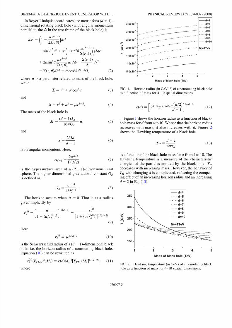
Figure 1 shows the horizon radius as a function of black-
hole mass for d from 4 to 10. We see that the horizon radius
increases with mass; it also increases with d. Figure 2
shows the Hawking temperature of a black hole
T H �dÿ 2
4rh(13)
as a function of the black-hole mass for d from 4 to 10. The
Hawking temperature is a measure of the characteristic
energies of the particles emitted by the black hole. T H decreases with increasing mass. However, the behavior of
T H with changing d is complicated, reflecting the compet-ing effect of an increasing horizon radius and an increasing
dÿ 2 in Eq. (13).
FIG. 1. Horizon radius (in GeVÿ1) of a nonrotating black hole
as a function of mass for 4–10 spatial dimensions.
FIG. 2. Hawking temperature (in GeV) of a nonrotating black
hole as a function of mass for 4–10 spatial dimensions.
BlackMax: A BLACK-HOLE EVENT GENERATOR WITH . . . PHYSICAL REVIEW D 77, 076007 (2008)
076007-3

8/3/2019 BlackMax Final
http://slidepdf.com/reader/full/blackmax-final 4/29
For the model with nonzero-tension brane, the radius of
the black hole is defined as
r�t�h � rs
B1=3 ; (14)
with B the deficit-angle parameter which is inverse pro-
portional to the tension of the brane.
Figure 3 shows the horizon radius as a function of black-
hole mass for the model with nonzero-tension brane. As the
deficit-angle parameter increases, the size of the black hole
increases.
Figure 4 shows the Hawking temperature of a black hole
for the model with nonzero-tension brane. The Hawking
temperature decreases as the deficit-angle decreases.Figure 5 shows the horizon radius as a function of black-
hole mass for a rotating black hole. The angular momen-
tum decreases the size of the horizon and increases the
Hawking temperature (see Figs. 5 and 6).If two highly relativistic particles collide with center-of-
mass energy ECM, and impact parameter b, then their
angular momentum in the center-of-mass frame before
the collision is Lin � bECM=2. Suppose for now that the
black hole that is formed retains all this energy and angular
momentum. Then the mass and angular momentum of the
black hole will be M in � ECM and J in � Lin. A black hole
will form if
b < bmax 2r�d�h �ECM ; bmaxECM=2�: (15)
We see that bmax is a function of both ECM and the number
of extra dimensions.
FIG. 3. Horizon radius (in GeVÿ1) of a black hole as a function
of mass for different B in d � 5 spatial dimensions.
FIG. 4. Hawking temperature (in GeV) of a black hole as a
function of mass for different B in d � 5 spatial dimensions.
FIG. 5. Horizon radius (in GeVÿ1) of a rotating black hole as a
function of mass for different angular momentum in d � 5spatial dimensions. Angular momentum J is in unit of @.
FIG. 6. Hawking temperature (in GeV) of a rotating black hole
as a function of mass for different angular momentum in d � 5spatial dimensions. Angular momentum J is in unit of @.
DE-CHANG DAI et al. PHYSICAL REVIEW D 77, 076007 (2008)
076007-4
8/3/2019 BlackMax Final
http://slidepdf.com/reader/full/blackmax-final 5/29
We can rewrite condition (15) as
bmax�ECM;d� � 2r�d�s �ECM�
�1 � �dÿ12�2�1=�dÿ2� : (16)
There is one exception to this condition. In the case
where we are including the effects of the brane tension,
the metric (and hence gray-body factors) for a rotating
black hole are not known. In this case we consider onlynonrotating black holes. Therefore, for branes with tension
btensionmax �ECM ; d� � 2r�d�s �ECM�: (17)
Also, for branes with tension only the d � 5 metric is
known.
At the LHC, each proton will have E � 7 TeV in the
CM frame. Therefore, the total proton-proton center-of-
mass energy will be���s
p � 14 TeV. However, it is not the
protons that collide to make the black holes, but the partons
of which the protons are made. If two partons have energy
vE and uEv
, much greater than their respective masses, then
the parton-parton collision will have
s0 � jpi � p jj2 �v�E;E� � u
v�E;ÿE�
2� 4uE2
� us: (18)
We define a quantity Q0
Q0 � ECM �����s0
p � �����
usp
: (19)
The center-of-mass energy for the two colliding partons
will be�����us
p , as will be the 4-momentum transfer Q02. The
largest impact parameter between the two partons that can
form a black hole with this mass will therefore be
bmax� �����usp ; d�, as given by Eq. (16).The total proton-proton cross section for black-hole
production is therefore
pp!BH �s; d;M ?� �Z 1M 2?=s
duZ 1u
dv
v �bmax�
�����us
p ; d��2
Xij
f i�v;Q0� f j�u=v;Q0�: (20)
Here f i�v;Q0� is the ith parton-distribution function.
Loosely this is the expected number of partons of type iand momentum vE to be found in the proton in a collision
at momentum transfer Q0.In [15], it is argued that strong gravity effects at energies
close to the Planck scale will lead to an increase in the 2 !2 cross section via the exchange of Planckian ‘‘black
holes’’ (by which any quantum-gravity effect or resonance
is meant). Final states with high multiplicities are predicted
to be suppressed. Although the intermediate state is created
in the strong gravity regime, it is not a conventional micro-scopic black hole. The state is not stable. Thermal
Hawking radiation does not take place. Especially since
inelastic collisions increase the energy loss, the threshold
for creating stable black holes shifts to even higher values.
Thus 2 ! 2 scattering may be the most important signal in
the LHC instead of black holes evaporating via Hawking
radiation. One should find that the cross section for two-
body final states suddenly jumps to a larger value, as the
energy reaches the quantum-gravity scale. We calculate the
cross section of two-body final states by replacingb2max in
Eq. (20) with
bmax�����s0p >M min�2 r2
sP2 ; (21)
where
P2 � eÿhN iX2
i�0
hN iii!
(22)
hN i �
4k�d�dÿ 1
M BH
M
�dÿ1�=�dÿ2�(23)
�Pcigiÿi �3�ÿ�3�
P ci f ii �4�ÿ�4�(24)
ÿi �1
4r2
Z i�!�!2d!
e!=T 1
Z !2d!
e!=T 1
ÿ1(25)
i �1
4r2
Z i�!�!3d!
e!=T 1
Z !3d!
e!=T 1
ÿ1: (26)
Here ci is the number of internal degrees of freedom of
particle species i, gi � 1 and f i � 1 for bosons, and gi �3=4 and f i � 7=8 for fermions [26].
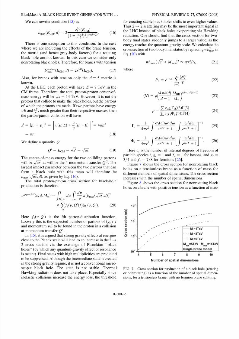
Figure 7 shows the cross section for nonrotating black
holes on a tensionless brane as a function of mass fordifferent numbers of spatial dimensions. The cross section
increases with the number of spatial dimensions.Figure 8 shows the cross section for nonrotating black
holes on a brane with positive tension as a function of mass
FIG. 7. Cross section for production of a black hole (rotating
or nonrotating) as a function of the number of spatial dimen-
sions, for a tensionless brane, with no fermion brane splitting.
BlackMax: A BLACK-HOLE EVENT GENERATOR WITH . . . PHYSICAL REVIEW D 77, 076007 (2008)
076007-5

8/3/2019 BlackMax Final
http://slidepdf.com/reader/full/blackmax-final 6/29
for various deficit-angle parameter, B. The cross section
increases as the tension increases (as B decreases).Figure 9 shows the cross section for nonrotating black
holes as a function of the number of split-fermion space
dimensions, ns. When a pair of partons are separated in the
extra dimensions they must approach more closely in the
ordinary dimensions in order to form a black hole. Thus,
the effective cross section for black-hole formation in
collisions is decreased. This effect becomes more severe
as ns increases because the partons are more likely to be
more widely separated in the extra dimensions, therefore
the cross section decreases with increasing ns.Figure 10 shows the cross section as a function of the
chosen minimum black-hole mass. The parton-distribution
functions strongly suppress the events with high black-holemasses.
Figure 11 shows the cross section for the two-body final-
state scenario as a function of the number of spatial di-
mensions, for M min � M � 1 TeV, M min � M �3 TeV, and M min � M � 5 TeV. It increases with the
number of spatial dimensions.
Black-hole formation in BlackMax
Within BlackMax, the probability of creating a black
hole of center-of-mass energy�����us
p , in the collision of two
protons of center-of-mass-energy ���sp
, is given by
FIG. 9. Cross section for production of a nonrotating black
hole as a function of the number of fermion brane-splitting
dimensions for d � 10.
FIG. 10. Cross section for formation of a black hole (rotating
or nonrotating) as a function of the minimum mass of black hole,
for a zero-tension brane, with no fermion brane splitting. The
vertical lines are the error bars.
FIG. 11. Cross section for the two-body final-state scenario as
a function of number of spatial dimensions where M min �M �1 TeV, M min �M � 3 TeV, and M min � 5 TeV.
FIG. 8. Cross section for production of a nonrotating black
hole as a function of the deficit-angle parameter for d � 5 and
ns � 2.
DE-CHANG DAI et al. PHYSICAL REVIEW D 77, 076007 (2008)
076007-6
8/3/2019 BlackMax Final
http://slidepdf.com/reader/full/blackmax-final 7/29
P�Q0� �Z 1u
dv
v
Xij
f i�v;Q0� f ju
v ;Q0
: (27)
According to the theory, there will be some minimum
mass for a black hole. We expect M min M , but leave
M min M as a free parameter. Therefore, a black hole
will only form if u > �M min=Q�2. The type of partons from
which a black hole is formed determines the gauge charges
of the black hole. Clearly, the probability to create a black hole in the collision of any two particular partons i and jwith energies (momenta) vE and uE
v is given by
P
vE;
uE
v;i ; j
� f i�v;Q0� f j�u=v;Q0�: (28)
The energies and types of the two colliding partons
determine their momenta and affect their locations within
the ordinary and extra dimensions. For protons moving in
the z-direction, we arbitrarily put one of the partons at the
origin and locate the second parton randomly within a disk
in the xy-plane of radius bmax�ECM �
�����us
p ; d�.
We must, however, also take into account that the par-
tons will be separated in the extra dimensions as well. Eachparton type is given awave function in the extra dimension.
For fermions, these wave functions are parametrized by
their centers and widths which are input parameters(cf. Fig. 14). In the split-fermion case, the centers of these
wave functions may be widely separated; but even in the
nonsplit case, the wave functions have nonzero widths. For
gauge bosons, the wave functions are taken to be constant
across the (thick) brane.
The output from the generator (described in greater de-
tail below) includes the energies, momenta, and types of
partons that yielded black holes. The locations in time and
space of the black holes are also output.
The formation of the black hole is a very nonlinear andcomplicated process. We assume that, before settling down
to a stationary phase, a black hole loses some fraction of its
energy, linear, and angular momentum. We parametrize
these losses by three parameters: 1 ÿ f E, 1 ÿ f P, and 1ÿ f L. Thus the black-hole initial state that we actually evolve
is characterized by
E � Ein f E; Pz � Pzin f P; J 0 � Lin f L; (29)
where Ein, Pzin, and Lin are initial energy, momentum, and
angular momentum of colliding partons, while f E, f P, and
f L are the fractions of the initial energy, momentum, and
angular momentum that are retained by the stationary
black hole. We expect that most of the energy lost in the
nonlinear regime is radiated in the form of gravitational
waves and thus represents missing energy. Yoshino and
Rychkov [43] have calculated the energy losses by numeri-
cal simulation of collisions. Their results will be incorpo-
rated in a future upgrade of BlackMax.
For a small black hole, the numerical value for the
angular momentum is of the order of several @. In that
range of values, angular momentum is quantized.
Therefore a black hole cannot have arbitrary values of
angular momentum. We keep the actual angular momen-
tum of the black hole, J , to be the nearest half-integer, i.e.
2J � �2J 0 � 12�.
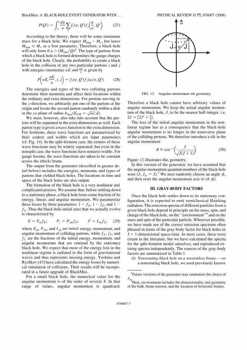
The loss of the initial angular momentum in the non-linear regime has as a consequence that the black-hole
angular momentum is no longer in the transverse plane
of the colliding protons. We therefore introduce a tilt in the
angular momentum
cosÿ1
J ������������������
J �J � 1�p : (30)
Figure 12 illustrates this geometry.
In this version of the generator, we have assumed that
the angular-momentum quantum numbers of the black hole
were (J , J m � J ).3 We next randomly choose an angle ,
and then reset the angular-momentum axis to
�;
�.
III. GRAY-BODY FACTORS
Once the black hole settles down to its stationary con-
figuration, it is expected to emit semiclassical Hawking
radiation. The emission spectra of different particles from a
given black hole depend in principle on the mass, spin, and
charge of the black hole, on the ‘‘environment’’4 and on the
mass and spin of the particular particle. Wherever possible,
we have made use of the correct emission spectrum often
phrased in terms of the gray-body factor for black holes in
3� 1-dimensional space-time. In most cases, these were
extant in the literature, but we have calculated the spectra
for the split-fermion model ourselves, and reproduced ex-isting spectra independently. The sources of the gray-body
factors are summarized in Table I.
(i) Nonrotating black hole on a tensionless brane.—or
a nonrotating black hole, we used previously known
Jm Jθ
ω
FIG. 12. Angular-momentum tilt geometry.
3Future versions of the generator may randomize the choice of
J m.4Here, environment includes the dimensionality and geometry
of the bulk, brane tension, and the location of fermionic branes.
BlackMax: A BLACK-HOLE EVENT GENERATOR WITH . . . PHYSICAL REVIEW D 77, 076007 (2008)
076007-7

8/3/2019 BlackMax Final
http://slidepdf.com/reader/full/blackmax-final 8/29
gray-body factors for spin 0, 1=2, and 1 fields in the
brane, and for spin 2 fields (i.e. gravitons) in the
bulk.
(ii) Rotating black hole on a tensionless brane.—For
rotating black holes, we used known gray-body fac-
tors for spin 0, 1=2, and 1 fields on the brane. The
correct emission spectrum for spin 2 bulk fields is not
yet known for rotating black holes; we currently do
not allow for the emission of bulk gravitons fromrotating black holes. As discussed below, this re-
mains a serious shortcoming of current micro-
black-hole phenomenology, since superradiance
might be expected to significantly increase graviton
emission from rotating black holes, and thus increase
the missing energy in a detector .
(iii) Nonrotating black holes on a tensionless brane with
fermion brane splitting.—In the split-fermion mod-
els, gauge fields can propagate through the bulk as
well as on the brane, so we have calculated gray-
body factors for spin 0 and 1 fields propagating
through the bulk, but only for a nonrotating black
hole for the split-fermion model. These are shown inFigs. 50–61.
(iv) Nonrotating black holes on a nonzero tension
brane.—The bulk gray-body factors for a brane
with nonzero tension are affected by nonzero tension
because of the modified bulk geometry (deficit
angle). We have calculated gray-body factors for
spin 0, 1, and 2 fields propagating through the
bulk, again only for the nonrotating black hole for
a brane with nonzero tension and d � 5.
(v) Two-particle final states.—We use the same gray-
body factors as a nonrotating black hole to calculate
the cross section of two-particle final states (exclud-
ing gravitons).
In all cases, the relevant emission spectra are loaded into
a data base as described in the Appendix.
IV. BLACK-HOLE EVOLUTION
The Hawking radiation spectra are calculated for the
black hole at rest in the center-of-mass frame of the collid-
ing partons. The spectra are then transformed to the labo-
ratory frame as needed. In all cases we have not (yet) taken
the charge of the black hole into account in calculating the
emission spectrum, but have included phenomenological
factors to account for it as explained below.
The degrees of freedom of the standard model particles
are given in Table II. Using the calculated Hawking spec-
trum and the number of degrees of freedom per particle, we
determine the expected radiated flux of each type of par-
ticle as a function of black-hole and environmental prop-erties. For each particle type i, we assign to it a specific
energy, @!i with a probability determined by that particle’s
emission spectrum. (The particle ‘‘types’’ are listed in
Table II.)
Assume a black hole with mass M bh emits a massless
particle with energy @!i. The remaining black hole will
have energy and momentum like
�M bh ÿ @!i ;ÿ@!i�: (31)
Here we ignore the other dimensions. We use a classical
model to simulate the events. The mass of the remaining
black hole should remain positive. So from Eq. (31) one
gets
@!i <M bh=2: (32)
Combining this with the observation that energy of a
TABLE I. Literature sources for particle emission spectra.
Type of particle Type of black hole Brane model References
Standard model particles Nonrotating Unsplit; tensionless [17,18]
Gravitons Nonrotating Split/unsplit; tensionless [16]
Standard model particles Nonrotating Split/unsplit; with tension [14]
Gravitons Nonrotating Split/unsplit; with tension [14]
Scalars and gauge bosons Nonrotating Split; tensionless Figs. 50–61
Fermions Rotating Unsplit; tensionless [22,23]
Gauge bosons Rotating Unsplit; tensionless [21,23]
Scalar fields Rotating Unsplit; tensionless [17,19,20,23]
TABLE II. Degrees of freedom of standard model particles
which are emitted from a black hole. For gravitons, the table
shows 1, because the appropriate growth in the number of
degrees of freedom is included explicitly in the graviton emis-
sion spectrum. ns is the number of extra dimensions in which
vector and scalar fields can propagate.
Particle type d0 d1=2 d1 d2
Quarks 0 6 0 0
Charged leptons 0 2 0 0
Neutrinos 0 2 0 0
Photons or gluons 0 0 2 � ns 0
Z 0 1 0 2 � ns 0
W � and W ÿ 2 0 2�2 � ns� 0
Higgs boson 1 0 0 0
Graviton 0 0 0 1
DE-CHANG DAI et al. PHYSICAL REVIEW D 77, 076007 (2008)
076007-8
8/3/2019 BlackMax Final
http://slidepdf.com/reader/full/blackmax-final 9/29
particle is larger than its mass leads us to require that
M i < @!i: (33)
We next need to determine whether that particle with
that energy is actually emitted within one generator time
step t. The time step itself is an input parameter
(cf. Fig. 14). We choose a random number N r from the
interval [0, 1]. Given LFi, the total number flux of particles
of type i, and N i, the number of degrees of freedom of thatparticle type, the particle will be emitted if
LFiN it > N r: (34)
In the single-brane model, LFi is derived from the power
spectrum of the Hawking radiation. In the split-fermion
model, we include a suppression factor for fermions. The
factor depends on the overlap between the particular fer-
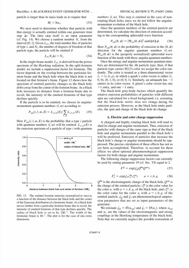
mion brane and the black hole when the black hole is notlocated on that fermion’s brane. Figure 13 shows how the
spectrum of emitted particles changes as the black hole
drifts away from the center of the fermion brane. As a black
hole increases its distance from a fermion brane due to
recoil, the intensity of the emitted fermions of that typedeclines quickly.
If the particle is to be emitted, we choose its angular-
momentum quantum numbers �l; m� according to
Pem�i;l ;m;E� � Li;l;m�E�=Xl0 ;m0
Li;l0 ;m0 �E�: (35)
Here Pem�i;l;m;E� is the probability that a type i particle
with quantum numbers �l; m� will be emitted. Li;l;m�E� is
the emission spectrum of a particle of type i with quantum
numbers �l; m�. This step is omitted in the case of non-
rotating black holes since we do not follow the angular-
momentum evolution of the black hole.
Once the quantum numbers of the emitted particle are
determined, we calculate the direction of emission accord-
ing to the corresponding spheroidal wave function:
Pem�;� � jlm�;�j2 sin: (36)
Here Pem�;� is the probability of emission in the �;�direction for the angular quantum numbers �‘;m�.lm�;� is the (properly normalized) spheroidal wavefunction of the mode with those angular quantum numbers.
Once the energy and angular-momentum quantum num-
bers are determined for the ith particle type, then, if that
particle type carries SU(3) color we assign the color ran-
domly. The color is treated as a three-dimensional vector
~ ci � �r;b;g�, in which a quark’s color-vector is either (1,
0, 0), (0, 1, 0), or (0, 0, 1). Similarly, an antiquark has ÿ1entries in its color-vector. A gluon’s color-vector has one
�1 entry, and one ÿ1 entry.
The black-hole gray-body factors which quantify the
relative emission probabilities of particles with differentspin are calculated for a fixed background, i.e. assuming
that the black-hole metric does not change during the
emission process. However, as the black hole emits parti-
cles, the spin and charge of the black hole do change.
A. Electric and color charge suppression
A charged and highly rotating black hole will tend to
shed its charge and angular momentum. Thus, emission of
particles with charges of the same sign as that of the black
hole and angular momentum parallel to the black hole’s
will be preferred. Emission of particles that increase the
black hole’s charge or angular momentum should be sup-pressed. The precise calculation of these effects has not as
yet been accomplished. Therefore, to account for these
effects we allow optional phenomenological suppression
factors for both charge and angular momentum.
The following charge-suppression factors can currently
be used by setting parameter 19 (cf. Sec. VI) equal to 2.
F Q � exp� QQbhQem� (37)
F 3a � exp� 3cbha c
ema � a � r;b;g: (38)
Qbh is the electromagnetic charge of the black hole, Qem is
the charge of the emitted particle; cbha is the color value for
the color a, with a � r;b;g, of the black hole, and cema , is
the color value for the color a, with a � r;b;g, of the
emitted particle. Q and 3 are phenomenological suppres-
sion parameters that are set as input parameters of the
generator.
We estimate Q � O�em� and 3 � O�s�, where em
and s are the values of the electromagnetic and strong
couplings at the Hawking temperature of the black hole.
Note that we currently neglect the possible restoration of
FIG. 13. The emitted fermion intensity (normalized to one) as
a function of the distance between the black hole and the center
of the Gaussian distribution of a fermionic brane. As a black hole
moves farther from a particular fermion brane due to recoil, the
intensity of emitted fermions of that type declines quickly. The
radius of black hole is set to be 2M ÿ1 . The width of the
fermionic brane is M ÿ1 . The plot is for the case of one extra
dimension.
BlackMax: A BLACK-HOLE EVENT GENERATOR WITH . . . PHYSICAL REVIEW D 77, 076007 (2008)
076007-9
8/3/2019 BlackMax Final
http://slidepdf.com/reader/full/blackmax-final 10/29
the electroweak symmetry in the vicinity of the black hole
when its Hawking temperature is above the electroweak
scale. Clearly, since em ’ 10ÿ2, we do not expect elec-
tromagnetic (or more correctly) electroweak charge sup-
pression to be a significant effect. However, since
s�1 TeV� ’ 0:1, color suppression may well play a role
in the evolution of the black hole.
Once we have determined the type of particle to be
emitted by the black hole, we draw a random number N rbetween 0 and 1 from a uniform distribution. If N r >F Q
then the emission process is allowed to occur, if N r <F Q
then the emission process is aborted. We repeat the same
procedure for color suppression factor, F 3a. Thus, particle
emission which decreases the magnitude of the charge or
color of the black hole is unsuppressed; this suppression
prevents the black hole from acquiring a large charge/
color, and gives preference to particle emission which
reduces the charge/color of the black hole.
B. Movement of the black hole during evaporation
We choose the direction of the momentum of the emittedparticle (P̂e) according to Eq. (36) in the center-of-mass
frame and then transform the energy and momentum to
their laboratory frame values @!0 and ~ P0e. The black-hole
properties (energy, momentum, mass, colors, and charge)
are then accordingly updated for the next time step:
E�t� t� � E�t� ÿ @!0 (39)
~ P�t� t� � ~ P�t� ÿ ~ P0e (40)
M �t� t� � ���������������������������������������������������E�t� t�2 ÿ ~ P�t� t�2q (41)
~ c bh�t� t� � ~ cbh�t� ÿ ci (42)
Qbh�t� t� � Qbh�t� ÿQi: (43)
Here ~ cbh is the color 3-vector of the black hole and can
have arbitrary integer entries.
Because of the recoil from the emitted particle, the black
hole will acquire a velocity ~ v and move to a position ~ x:
~ v�t� � ~ P�t�=E (44)
~ x
�t
�t
� �~ x
�t
� �~ v
�t
�t: (45)
Since fermions are constrained to live on the 3�1-dimensional regular brane, the recoil from fermions is
not important. Only the emission of vector fields, scalar
fields, and gravitons gives a black-hole momentum in extra
dimension. Once a black hole gains momentum in extra
dimension, it is able to leave the regular brane if it carries
no gauge charge. In the split-fermion case, it can move
within the minibulk even if it carries gauge charge. In the
case of rotating black holes, because the gray-body factor
for gravitons is not yet known, graviton emission is turned
off in the generator and the black holes experience no bulk
recoil.
Recoil can in principle change the radiation spectrum of
the black hole in two ways. First, the spectrum will not be
perfectly thermal or spherically symmetric in the labora-
tory frame, but rather boosted due to the motion of the
black hole. However, as we shall see, the black hole never
becomes highly relativistic, so the recoil does not signifi-cantly affect the shape of the spectrum.
As the lifetime of a small black hole is relatively short,and its recoil velocity nonrelativistic, it does not move far
from its point of creation. However, even a recoil of the
order of 1 fundamental length M ÿ1 in the bulk direction
could dislocate the black hole from the brane.5 In single-
brane models this would result in apparent missing energy
for an observer located on the brane able to detect only
standard model particles. In the split-fermion model, as the
black hole moves off or on particular fermion branes, thedecay channels open to it will change.
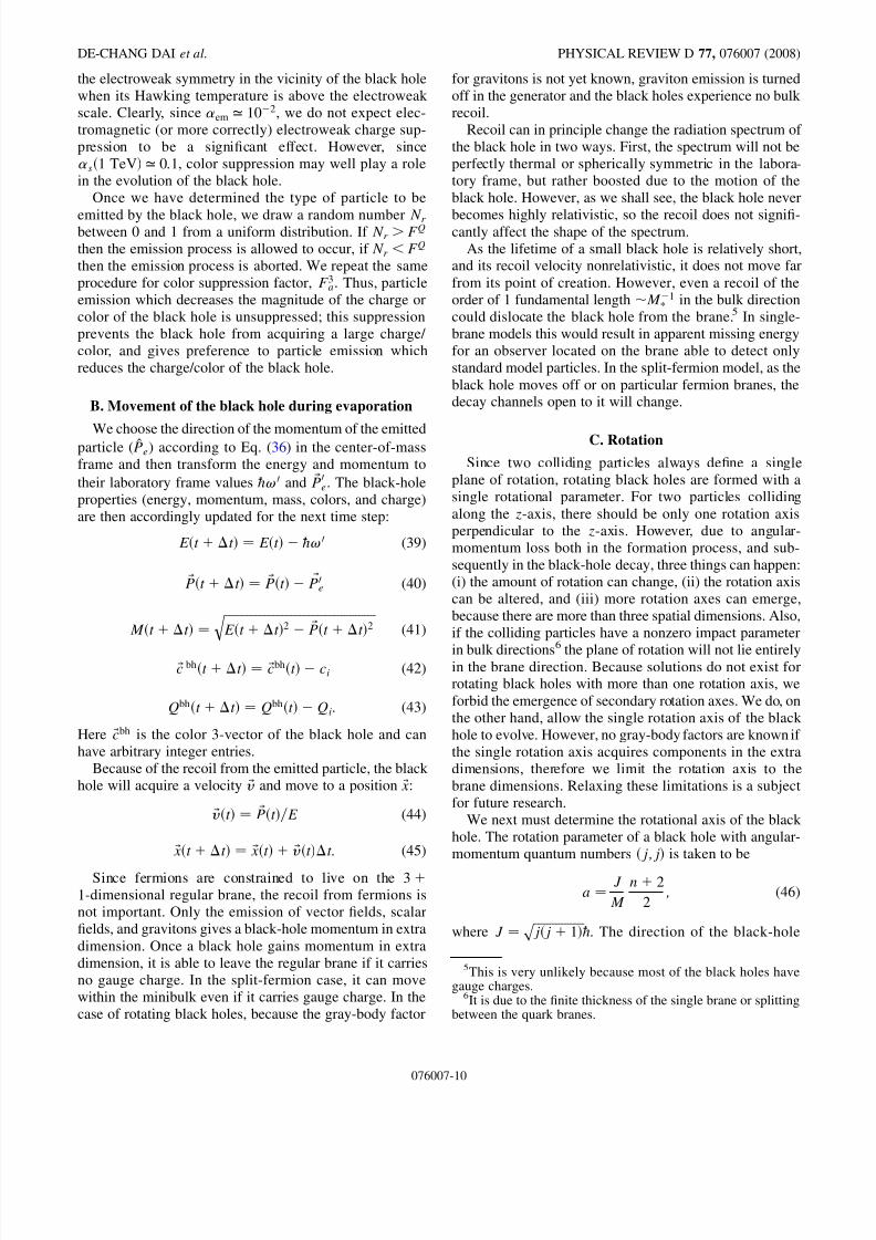
C. Rotation
Since two colliding particles always define a single
plane of rotation, rotating black holes are formed with a
single rotational parameter. For two particles colliding
along the z-axis, there should be only one rotation axis
perpendicular to the z-axis. However, due to angular-
momentum loss both in the formation process, and sub-
sequently in the black-hole decay, three things can happen:
(i) the amount of rotation can change, (ii) the rotation axis
can be altered, and (iii) more rotation axes can emerge,
because there are more than three spatial dimensions. Also,
if the colliding particles have a nonzero impact parameter
in bulk directions6
the plane of rotation will not lie entirelyin the brane direction. Because solutions do not exist forrotating black holes with more than one rotation axis, we
forbid the emergence of secondary rotation axes. We do, on
the other hand, allow the single rotation axis of the black
hole to evolve. However, no gray-body factors are known if
the single rotation axis acquires components in the extra
dimensions, therefore we limit the rotation axis to the
brane dimensions. Relaxing these limitations is a subject
for future research.
We next must determine the rotational axis of the black
hole. The rotation parameter of a black hole with angular-
momentum quantum numbers
� j;j
�is taken to be
a � J
M
n� 2
2; (46)
where J � ����������������� j� j� 1�p
@. The direction of the black-hole
5This is very unlikely because most of the black holes have
gauge charges.6It is due to the finite thickness of the single brane or splitting
between the quark branes.
DE-CHANG DAI et al. PHYSICAL REVIEW D 77, 076007 (2008)
076007-10
8/3/2019 BlackMax Final
http://slidepdf.com/reader/full/blackmax-final 11/29
angular momentum is taken to be
~ J � j@!̂� ��� jp
@l̂? ; (47)
where l̂? is a unit vector in the plane perpendicular to !̂.
We chose the direction of l̂? randomly.
When the black hole emits a particle with angular-
momentum quantum numbers �l; m�, there are several pos-
sible final states in which the black hole can end up. We use
Clebsch-Gordan coefficients to find the probability of each
state:
j j;ji �Xj jÿlj
j0 j�lC� j;j; l;m;j0 ; jÿm�jl; mij j0 ; jÿmi: (48)
We use jC� j;j; l;m;j0 ; jÿm�j2 as the probability that
the new angular-momentum quantum numbers of the black
hole will be � j0 ; jÿm�. From angular-momentum conser-
vation ~ J � ~ L� ~ J 0, we can calculate the tilt angle of the
black-hole rotation axis as
cos � j� j�
1� �
j0� j0�
1� ÿ
l�l�
1�2
������������������������������������ j� j� 1� j0� j0 � 1�p : (49)
We randomly choose a direction with the tilt angle as a
new rotation axis and change quantum numbers to � j0 ; j0�.In calculating the gray-body factors, the black hole is
always treated as a fixed unchanging background. The
power spectrum of emitted particles can be calculated from
dE
dt�Xl;m
j Al;mj2!
exp��!ÿm�=T H � 1
d!
2 : (50)
Here l and m are angular-momentum quantum numbers. !is the energy of the emitted particle. is defined by
� a�1� a2�rh
: (51)
The exponential factor in the denominator of (50) causes
the black hole to prefer to emit high angular-momentum
particles. However, since the TeV black holes are quantum
black holes, the gray-body factors should really depend on
both the initial and final black-hole parameters. The cal-
culation of the gray-body spectra on a fixed background
can cause some problems. In particular, in the current case,
the angular momentum of the emitted particle (as indeed
the energy) may well be comparable to that of the black
hole itself. There should be a suppression of particle emis-
sion processes in which the black-hole final state is very
different from the initial state. We therefore introduce a
new phenomenological suppression factor, parameter 17,
to reduce the probability of emission events in which the
angular momentum of the black hole changes by a large
amount.
If parameter 17 is equal to 1 (cf. Sec. VI), we do not take
into account the suppression of decays which increase the
angular momentum of the black hole. If we are using
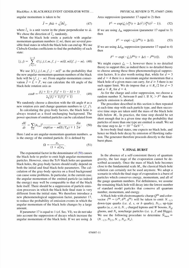
Area suppression (parameter 17 equal to 2) then
F L � exp� L�rbhh �t� t�2=rbh
h �t�2 ÿ 1��: (52)
If we are using J bh suppression (parameter 17 equal to 3)
then
F L � exp�ÿ LjJ bh�t� t�j�: (53)
If we are using J bh suppression (parameter 17 equal to 4)then
F L � exp�ÿ LjJ bh�t� t� ÿ J bh�t�j�: (54)
We might expect L 1, however there is no detailed
theory to support this; as indeed there is no detailed theory
to choose among these three phenomenological suppres-
sion factors. It is also worth noting that, while for d � 3and d � 4 there is a maximum angular momentum that a
black hole of a given mass can carry, for d 5 there is no
such upper limit. We do impose that a Rs=2 for d � 3and a Rs for d � 4.
As for the charge and color suppression, we choose arandom number N r between 0 and 1. If N r >F L then the
particle emission is aborted.
The procedure described in this section is then repeated
at each time step with each particle type, and then succes-
sive time steps are taken until the mass of the black hole
falls below M . In practice, the time step should be set
short enough that in a given time step the probability that
particles of more than one type are emitted is small. We set
the time step to t � 10ÿ5 GeVÿ1.In two-body final states, one expects no black hole, and
hence no black-hole decay by emission of Hawking radia-
tion. The generator therefore proceeds directly to the final-
burst phase.
V. FINAL BURST
In the absence of a self-consistent theory of quantum
gravity, the last stage of the evaporation cannot be de-
scribed accurately. Once the mass of black hole becomes
close to the fundamental scale M , the classical black-hole
solution can certainly not be used anymore. We adopt a
scenario in which the final stage of evaporation is a burst of
particles which conserves energy, momentum, and all of
the gauge quantum numbers. For definiteness, we assume
the remaining black hole will decay into the lowest number
of standard model particles that conserve all quantumnumber, momentum, and energy.
A black hole with electromagnetic chargeQbh and color-
vector ~ cbh � �rbh ; bbh ; gbh� will be taken to emit N ÿ1=3
down-type quarks (i.e. d, s, or b quarks), N 2=3 up-type
quarks (u, c, or t), N ÿ1 charged leptons and W bosons, N gl
gluons, and N n noncharge particles (i.e. , Z and Higgs).
We use the following procedure to determine ~ N burst �N ÿ1=3 ; N 2=3 ; N ÿ1 ; N gl ; N n�.
BlackMax: A BLACK-HOLE EVENT GENERATOR WITH . . . PHYSICAL REVIEW D 77, 076007 (2008)
076007-11

8/3/2019 BlackMax Final
http://slidepdf.com/reader/full/blackmax-final 12/29
Step 1: preliminary solution:
(i) Search all possible solutions with N n � 0.
(ii) Choose the minimum number of particles as prelimi-
nary solution.
Step 2: Actual charged/colored emitted particle count:
(i) The preliminary ~ N burst�N ÿ1=3 ;N 2=3 ;N ÿ1 ;N gl ;N n�having now been determined. If the minimum num-
ber of solution is less than 2, we then add N n to keep
the total number equal to 2. Later we choose one of them randomly according to the degrees of freedom
of each particle.
(ii) After obtaining the number of emitted particles, we
randomly assign their energies and momenta, subject
to the constraint that the total energy and momentum
equal that of the final black-hole state. We currently
neglect any bulk components of the final black-hole
momentum.
VI. INPUT AND OUTPUT
The input parameters for the generator are read from the
file parameter.txt, see Fig. 14:
(1) Numberofsimulations: sets the total number
of black-hole events to be simulated;
(2) Centerof massenergyofprotons: sets the
center-of-mass energy of the colliding protons in
GeV;(3) Mph: sets the fundamental quantum-gravity scale
(M ) in GeV;
(4) Chooseacase: defines the extra-dimension model
to be simulated:
(a) 1: nonrotating black holes on a tensionless
brane with possibility of fermion splitting,
(b) 2: nonrotating black holes on a brane with
nonzero positive tension,
FIG. 14. Parameter.txt is the input file containing the parameters that one can change. The words in parentheses are the parameters
that are used in the paper.
DE-CHANG DAI et al. PHYSICAL REVIEW D 77, 076007 (2008)
076007-12
8/3/2019 BlackMax Final
http://slidepdf.com/reader/full/blackmax-final 13/29
(c) 3: rotating black holes on a tensionless branewith d � 5,
(d) 4: two-particle final-state scenario;
(5) numberofextradimensions: sets the number
of extra dimensions; this must equal 2 for brane with
tension (Chooseacase � 2);
(6) numberofsplittingdimensions: sets the
number of extra split-fermion dimensions
(Chooseacase � 1);
(7) extradimensionsize: sets the size of the mini-
bulk 7 in units of 1=TeV (Chooseacase � 1);
(8) tension: sets the deficit-angle parameter B[13,14] (Choose
a
case
�2);
(9) chooseapdffile: defines which of the different
CTEQ6 parton-distribution functions (PDF) to use;
(10) Minimum mass: sets the minimum mass M min in
GeV of the initial black holes;
(11) fixtimestep: If equal to 1, then code uses the
next parameter to determine the time interval be-tween events; if equal to 2 then code tries to opti-
mize the time step, keeping the probability of
emitting a particle in any given time step below
10%.
(12) timestep: defines the time interval t in GeVÿ1
which the generator will use for the black-hole
evolution;
(13) Masslossfactor: sets the loss factor 0 for the
energy of the initial black hole, as defined in
Eq. (29);
(14) momentumlossfactor: defines the loss factor
0 f p
1 for the momentum of initial black holes
as defined in Eq. (29);
(15) Angular momentumlossfactor: sets the loss
factor 0 f L 1 for the angular momentum of
initial black holes is defined in Eq. (29);
(16) Seed: sets the seed for the random-number genera-
tor (9 digit positive integer);
(17) Lsuppression: chooses the model for suppress-
ing the accumulation of large black-hole angular
momenta during the evolution phase of the black
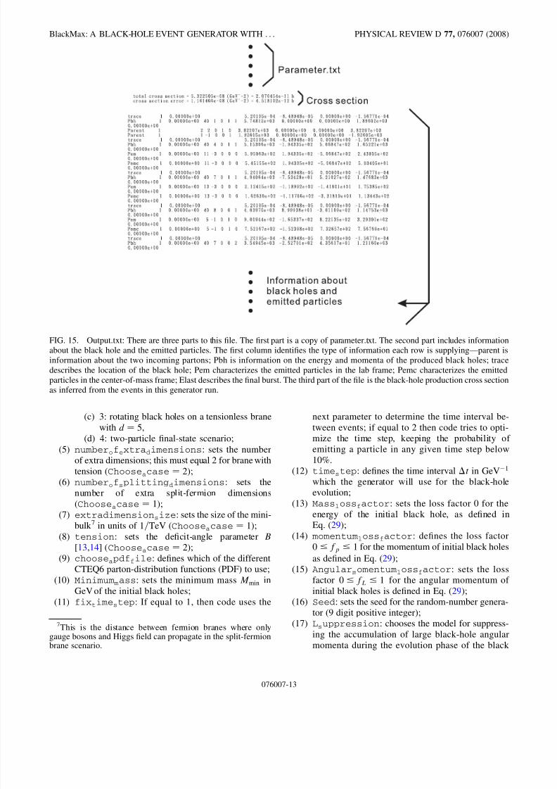
FIG. 15. Output.txt: There are three parts to this file. The first part is a copy of parameter.txt. The second part includes information
about the black hole and the emitted particles. The first column identifies the type of information each row is supplying—parent is
information about the two incoming partons; Pbh is information on the energy and momenta of the produced black holes; trace
describes the location of the black hole; Pem characterizes the emitted particles in the lab frame; Pemc characterizes the emitted
particles in the center-of-mass frame; Elast describes the final burst. The third part of the file is the black-hole production cross section
as inferred from the events in this generator run.
7This is the distance between fermion branes where only
gauge bosons and Higgs field can propagate in the split-fermionbrane scenario.
BlackMax: A BLACK-HOLE EVENT GENERATOR WITH . . . PHYSICAL REVIEW D 77, 076007 (2008)
076007-13
8/3/2019 BlackMax Final
http://slidepdf.com/reader/full/blackmax-final 14/29
holes [cf. discussion surrounding Eqs. (52)–(54)];
(a) 1: no suppression;
(b) 2: Area suppression;
(c) 3: J bh suppression;(d) 4: J suppression;
(18) angular momentumsuppressionfactor: de-
fines the phenomenological angular-momentum
suppression factor, L [cf. discussion surrounding
Eq. (52)–(54)];
(19) chargesuppression: turns the suppression of
accumulation of large black-hole electromagnetic
and color charge during the black-hole evolution
process on or off [cf. discussion surrounding
Eq. (37)]
(a) 0: charge suppression turned off;
(b) 1: charge suppression turned on;
(20) chargesuppressionfactor: sets the electro-magnetic charge-suppression factor, Q, in (37);
(21) colorsuppressionfactor: sets the color
charge-suppression factor, 3 in (37);
21–94 (odd entries): the widths of fermion wave functions
(in M ÿ1 units); and (even entries:) centers of fermion wave
functions (in M ÿ1 units) in split-brane models, represented
as 9-dimensional vectors (for nonsplit models, set all en-
tries to 0).
When the code terminates, the file output.txt (Fig. 15)
with all the relevant information (i.e. input parameters,
cross section) is output to the working directory. This file
contains also different segments of information about the
generation of black holes which are labeled at the begin-
ning of each line with an ID word (Parent, Pbh, trace, Pem,
Pemc, or Elast):
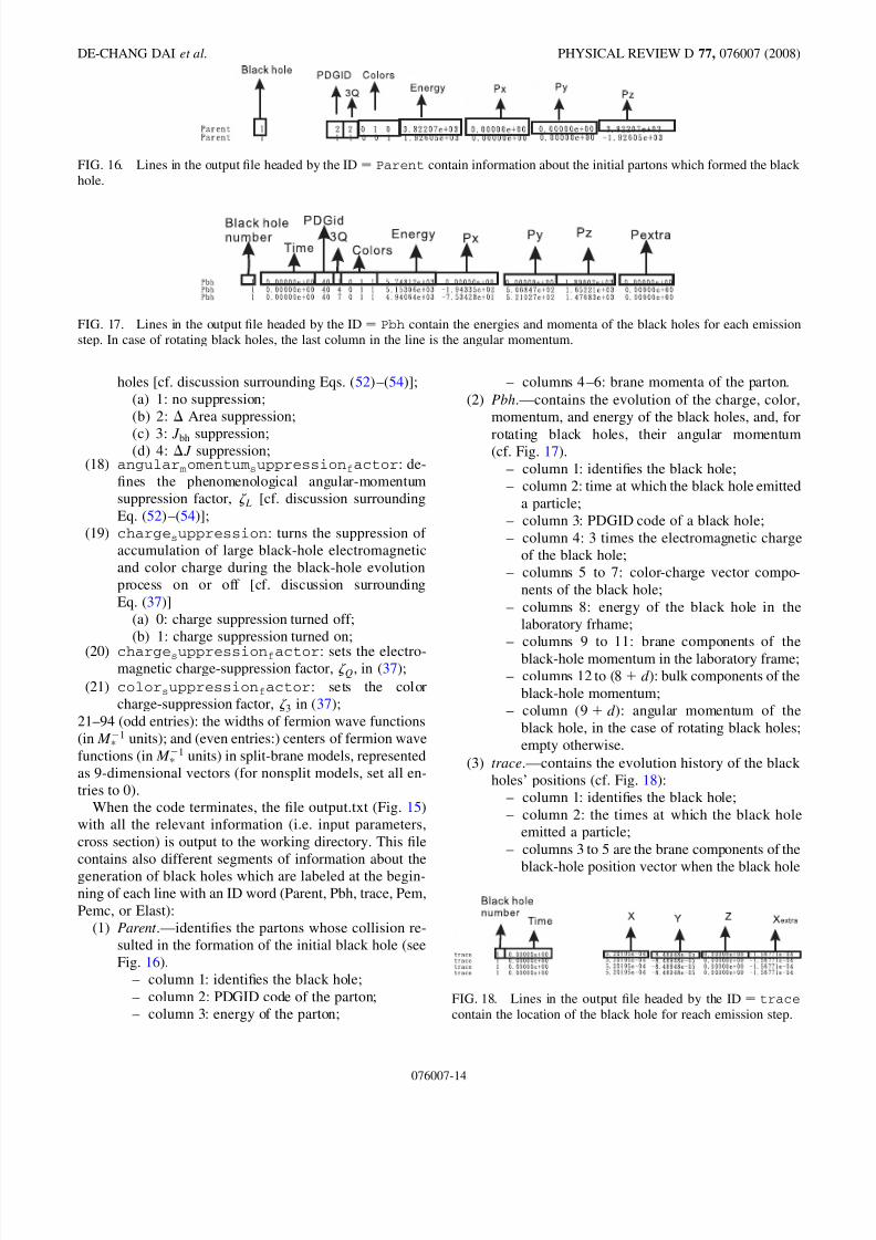
(1) Parent .—identifies the partons whose collision re-
sulted in the formation of the initial black hole (see
Fig. 16).
– column 1: identifies the black hole;
– column 2: PDGID code of the parton;
– column 3: energy of the parton;
– columns 4–6: brane momenta of the parton.
(2) Pbh.—contains the evolution of the charge, color,
momentum, and energy of the black holes, and, for
rotating black holes, their angular momentum(cf. Fig. 17).
– column 1: identifies the black hole;
– column 2: time at which the black hole emitted
a particle;
– column 3: PDGID code of a black hole;
– column 4: 3 times the electromagnetic charge
of the black hole;
– columns 5 to 7: color-charge vector compo-
nents of the black hole;
– columns 8: energy of the black hole in the
laboratory frhame;
– columns 9 to 11: brane components of the
black-hole momentum in the laboratory frame;
– columns 12 to (8 � d): bulk components of the
black-hole momentum;
– column (9 � d): angular momentum of the
black hole, in the case of rotating black holes;
empty otherwise.
(3) trace.—contains the evolution history of the black
holes’ positions (cf. Fig. 18):
– column 1: identifies the black hole;
– column 2: the times at which the black hole
emitted a particle;
– columns 3 to 5 are the brane components of the
black-hole position vector when the black hole
FIG. 16. Lines in the output file headed by the ID � Parent contain information about the initial partons which formed the black
hole.
FIG. 17. Lines in the output file headed by the ID � Pbh contain the energies and momenta of the black holes for each emission
step. In case of rotating black holes, the last column in the line is the angular momentum.
FIG. 18. Lines in the output file headed by the ID � tracecontain the location of the black hole for reach emission step.
DE-CHANG DAI et al. PHYSICAL REVIEW D 77, 076007 (2008)
076007-14
8/3/2019 BlackMax Final
http://slidepdf.com/reader/full/blackmax-final 15/29
emitted a particle;
– columns 6 to (2� d): the bulk components of the black-hole position vector, when the black
hole emitted a particle.
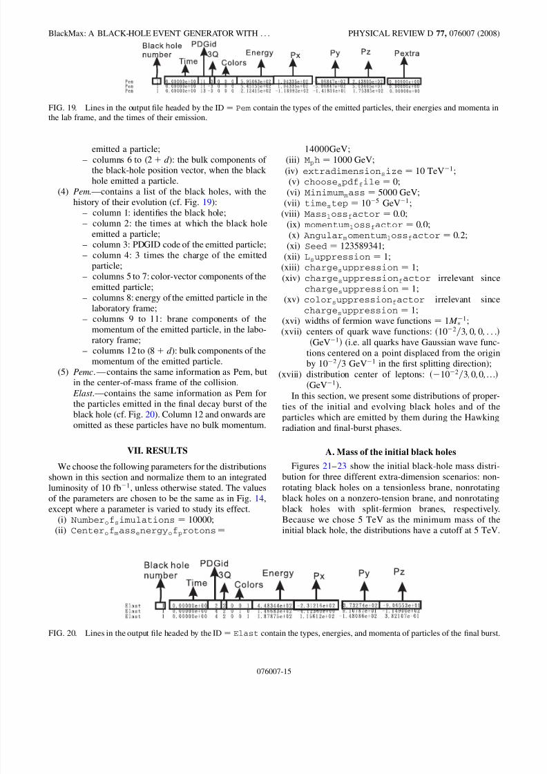
(4) Pem.—contains a list of the black holes, with the
history of their evolution (cf. Fig. 19):
– column 1: identifies the black hole;
– column 2: the times at which the black hole
emitted a particle;
– column 3: PDGID code of the emitted particle;
– column 4: 3 times the charge of the emitted
particle;
– columns 5 to 7: color-vector components of the
emitted particle;
– columns 8: energy of the emitted particle in the
laboratory frame;
– columns 9 to 11: brane components of the
momentum of the emitted particle, in the labo-
ratory frame;
– columns 12 to (8� d): bulk components of the
momentum of the emitted particle.
(5) Pemc.—contains the same information as Pem, but
in the center-of-mass frame of the collision.
Elast .—contains the same information as Pem for
the particles emitted in the final decay burst of theblack hole (cf. Fig. 20). Column 12 and onwards are
omitted as these particles have no bulk momentum.
VII. RESULTS
We choose the following parameters for the distributions
shown in this section and normalize them to an integrated
luminosity of 10 fbÿ1, unless otherwise stated. The values
of the parameters are chosen to be the same as in Fig. 14,
except where a parameter is varied to study its effect.
(i) Numberofsimulations � 10000;
(ii) Centerof massenergyofprotons�
14000GeV;
(iii) Mph � 1000 GeV;
(iv) extradimensionsize � 10 TeVÿ1;
(v) chooseapdffile � 0;
(vi) Minimum mass � 5000 GeV;
(vii) timestep � 10ÿ5 GeVÿ1;
(viii) Masslossfactor � 0:0;
(ix) momentumlossfactor � 0:0;
(x) Angular momentumlossfactor � 0:2;
(xi) Seed � 123589341;
(xii) Lsuppression � 1;
(xiii) chargesuppression � 1;(xiv) chargesuppressionfactor irrelevant since
chargesuppression � 1;
(xv) colorsuppressionfactor irrelevant since
chargesuppression � 1;
(xvi) widths of fermion wave functions � 1M ÿ1 ;
(xvii) centers of quark wave functions: �10ÿ2=3 ; 0 ; 0 ; . . .��GeVÿ1� (i.e. all quarks have Gaussian wave func-
tions centered on a point displaced from the origin
by 10ÿ2=3 GeVÿ1 in the first splitting direction);
(xviii) distribution center of leptons: �ÿ10ÿ2=3 ;0 ;0 ;. . .��GeVÿ1�.
In this section, we present some distributions of proper-
ties of the initial and evolving black holes and of theparticles which are emitted by them during the Hawking
radiation and final-burst phases.
A. Mass of the initial black holes
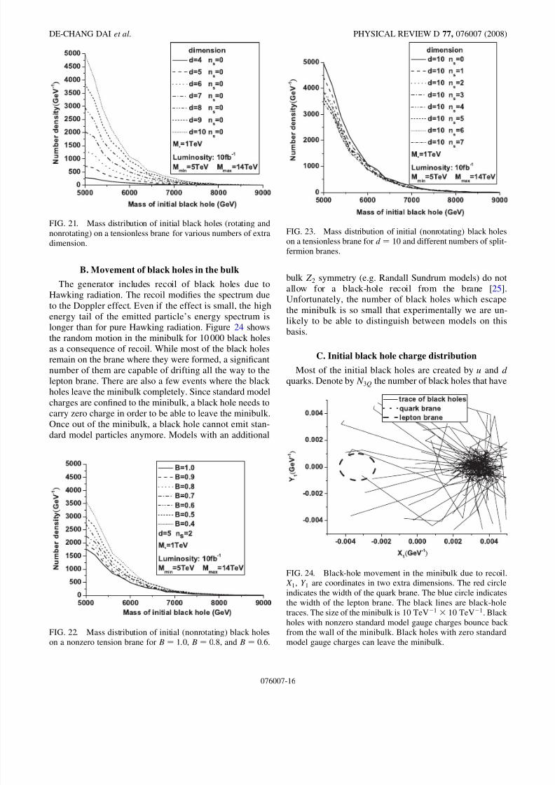
Figures 21–23 show the initial black-hole mass distri-
bution for three different extra-dimension scenarios: non-
rotating black holes on a tensionless brane, nonrotating
black holes on a nonzero-tension brane, and nonrotating
black holes with split-fermion branes, respectively.
Because we chose 5 TeV as the minimum mass of the
initial black hole, the distributions have a cutoff at 5 TeV.
FIG. 19. Lines in the output file headed by the ID � Pem contain the types of the emitted particles, their energies and momenta in
the lab frame, and the times of their emission.
FIG. 20. Lines in the output file headed by the ID � Elast contain the types, energies, and momenta of particles of the final burst.
BlackMax: A BLACK-HOLE EVENT GENERATOR WITH . . . PHYSICAL REVIEW D 77, 076007 (2008)
076007-15
8/3/2019 BlackMax Final
http://slidepdf.com/reader/full/blackmax-final 16/29
B. Movement of black holes in the bulk
The generator includes recoil of black holes due to
Hawking radiation. The recoil modifies the spectrum due
to the Doppler effect. Even if the effect is small, the high
energy tail of the emitted particle’s energy spectrum is
longer than for pure Hawking radiation. Figure 24 shows
the random motion in the minibulk for 10 000 black holes
as a consequence of recoil. While most of the black holes
remain on the brane where they were formed, a significant
number of them are capable of drifting all the way to the
lepton brane. There are also a few events where the black
holes leave the minibulk completely. Since standard model
charges are confined to the minibulk, a black hole needs to
carry zero charge in order to be able to leave the minibulk.Once out of the minibulk, a black hole cannot emit stan-
dard model particles anymore. Models with an additional
bulk Z 2 symmetry (e.g. Randall Sundrum models) do notallow for a black-hole recoil from the brane [25].Unfortunately, the number of black holes which escape
the minibulk is so small that experimentally we are un-
likely to be able to distinguish between models on this
basis.
C. Initial black hole charge distribution
Most of the initial black holes are created by u and dquarks. Denote by N 3Q the number of black holes that have
FIG. 23. Mass distribution of initial (nonrotating) black holes
on a tensionless brane for d � 10 and different numbers of split-
fermion branes.
FIG. 22. Mass distribution of initial (nonrotating) black holes
on a nonzero tension brane for B � 1:0, B � 0:8, and B � 0:6.
FIG. 21. Mass distribution of initial black holes (rotating and
nonrotating) on a tensionless brane for various numbers of extra
dimension.
FIG. 24. Black-hole movement in the minibulk due to recoil.
X 1, Y 1 are coordinates in two extra dimensions. The red circle
indicates the width of the quark brane. The blue circle indicates
the width of the lepton brane. The black lines are black-hole
traces. The size of the minibulk is 10 TeVÿ1 10 TeVÿ1. Black
holes with nonzero standard model gauge charges bounce back
from the wall of the minibulk. Black holes with zero standard
model gauge charges can leave the minibulk.
DE-CHANG DAI et al. PHYSICAL REVIEW D 77, 076007 (2008)
076007-16
8/3/2019 BlackMax Final
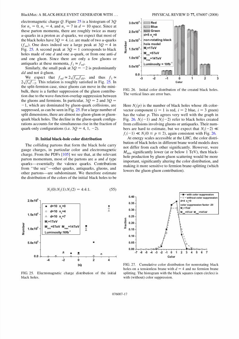
http://slidepdf.com/reader/full/blackmax-final 17/29
electromagnetic charge Q. Figure 25 is a histogram of 3Qfor ns � 0, ns � 4, and ns � 7 in d � 10 space. Since at
these parton momenta, there are roughly twice as many
u-quarks in a proton as d-quarks, we expect that most of
the black holes have 3Q � 4. i.e. are made of two u-quarks
( f uu). One does indeed see a large peak at 3Q � 4 in
Fig. 25. A second peak at 3Q � 1 corresponds to black
holes made of one d and one u-quark, or from one anti-d
and one gluon. Since there are only a few gluons orantiquarks at these momenta, f 1 ’ f ud.
Similarly, the small peak at 3Q � ÿ2 is predominantly
dd and not u-gluon.
We expect that f ud ’ 2�������������� f uu f ddp
, and thus f 1 ’2������������� f 4 f ÿ2
p . This relation is roughly satisfied in Fig. 25. In
the split-fermion case, since gluons can move in the mini-
bulk, there is a further suppression of the gluon contribu-
tion due to the wave-function-overlap suppression between
the gluons and fermions. In particular, 3Q � 2 and 3Q �ÿ1, which are dominated by gluon-quark collisions, aresuppressed, as can be seen in Fig. 25. For a large number of
split dimensions, there are almost no gluon-gluon or gluon-
quark black holes. The decline in the gluon-quark configu-rations accounts for the simultaneous rise in the fraction of
quark-only configurations (i.e. 3Q � 4, 1, ÿ2).
D. Initial black-hole color distribution
The colliding partons that form the black hole carry
gauge charges, in particular color and electromagnetic
charge. From the PDFs [105] we see that, at the relevant
parton momentum, most of the partons are u and d type
quarks—essentially the valence quarks. Contributions
from ‘‘the sea’’—other quarks, antiquarks, gluons, and
other partons—are subdominant. We therefore estimate
the distribution of the colors of the initial black holes to be
N i�0�:N i�1�:N i�2� � 4:4:1: (55)
Here N i�p� is the number of black holes whose ith color-
vector component (i � 1 is red, i � 2 blue, i � 3 green)
has the value p. This agrees very well with the graph in
Fig. 26. N i�ÿ1� and N i�ÿ2� refer to black holes createdfrom collisions involving gluons or antiquarks. Their num-
bers are hard to estimate, but we expect that N i�ÿ2� f i�ÿ1� N i�0 p 2�, again consistent with Fig. 26.
At energy scales accessible at the LHC, the color distri-
bution of black holes in different brane world models does
not differ from each other significantly. However, were
M min significantly lower (at or below 1 TeV), then black-
hole production by gluon-gluon scattering would be more
important, significantly altering the color distribution, and
making it more sensitive to fermion brane-splitting (which
lowers the gluon-gluon contribution).
FIG. 25. Electromagnetic charge distribution of the initial
black holes.
FIG. 26. Initial color distribution of the created black holes.
The vertical lines are error bars.
FIG. 27. Cumulative color distribution for nonrotating black
holes on a tensionless brane with d � 4 and no fermion brane
splitting. The histogram with the black squares (open circles) is
with (without) color suppression.
BlackMax: A BLACK-HOLE EVENT GENERATOR WITH . . . PHYSICAL REVIEW D 77, 076007 (2008)
076007-17
8/3/2019 BlackMax Final
http://slidepdf.com/reader/full/blackmax-final 18/29
E. Evolution of black-hole color and charge during the
Hawking radiation phase
Figure 27 shows the color distribution of the black holes
which they accumulate during the evaporation phase. From
Eq. (55), the expected average initial color of the black holes is 2=3. Since the colors of emitted particles are
assigned randomly, we expect the cumulative color distri-
bution (CCD) to be symmetric around 2=3 and peaked at
the value. This is indeed what we find.The width of the CCD depends on the total number of
particles emitted by the black hole during its evaporation
phase.
As discussed above, we allow for the possibility of
suppressing particle emission which increases the charge,
color, or angular momentum of the black hole excessively
[cf. discussion around Eqs. (37) and (52)–(54)]. Figure 27
shows also the cumulative black-hole color distribution
where we suppressed the accumulation of large color
charges during the evaporation phase. In order to amplify
the effect of color suppression, we have set f 3 � 20 instead
of the expected f 3’
0:1. We see that the number of black
holes with a color charge larger than 1 is decreased.
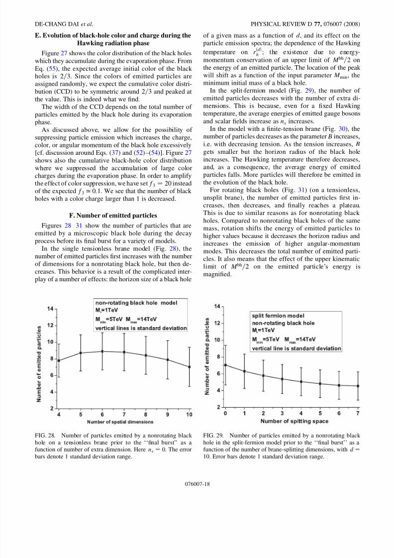
F. Number of emitted particles
Figures 28–31 show the number of particles that are
emitted by a microscopic black hole during the decay
process before its final burst for a variety of models.
In the single tensionless brane model (Fig. 28), the
number of emitted particles first increases with the number
of dimensions for a nonrotating black hole, but then de-
creases. This behavior is a result of the complicated inter-
play of a number of effects: the horizon size of a black hole
of a given mass as a function of d, and its effect on the
particle emission spectra; the dependence of the Hawking
temperature on r�d�h ; the existence due to energy-
momentum conservation of an upper limit of M bh=2 on
the energy of an emitted particle. The location of the peak
will shift as a function of the input parameter M min, the
minimum initial mass of a black hole.
In the split-fermion model (Fig. 29), the number of
emitted particles decreases with the number of extra di-mensions. This is because, even for a fixed Hawking
temperature, the average energies of emitted gauge bosons
and scalar fields increase as ns increases.
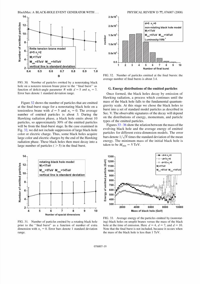
In the model with a finite-tension brane (Fig. 30), thenumber of particles decreases as the parameter B increases,
i.e. with decreasing tension. As the tension increases, Bgets smaller but the horizon radius of the black hole
increases. The Hawking temperature therefore decreases,
and, as a consequence, the average energy of emitted
particles falls. More particles will therefore be emitted in
the evolution of the black hole.
For rotating black holes (Fig. 31) (on a tensionless,
unsplit brane), the number of emitted particles first in-creases, then decreases, and finally reaches a plateau.
This is due to similar reasons as for nonrotating black
holes. Compared to nonrotating black holes of the same
mass, rotation shifts the energy of emitted particles to
higher values because it decreases the horizon radius and
increases the emission of higher angular-momentum
modes. This decreases the total number of emitted parti-
cles. It also means that the effect of the upper kinematic
limit of M bh=2 on the emitted particle’s energy is
magnified.
FIG. 28. Number of particles emitted by a nonrotating black
hole on a tensionless brane prior to the ‘‘final burst’’ as a
function of number of extra dimension. Here ns � 0. The error
bars denote 1 standard deviation range.
FIG. 29. Number of particles emitted by a nonrotating black
hole in the split-fermion model prior to the ‘‘final burst’’ as a
function of the number of brane-splitting dimensions, with d �10. Error bars denote 1 standard deviation range.
DE-CHANG DAI et al. PHYSICAL REVIEW D 77, 076007 (2008)
076007-18
8/3/2019 BlackMax Final
http://slidepdf.com/reader/full/blackmax-final 19/29
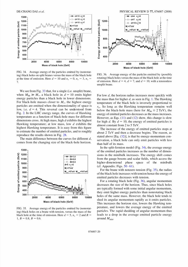
Figure 32 shows the number of particles that are emitted
at the final-burst stage for a nonrotating black hole on a
tensionless brane with d � 5 and ns � 0. The average
number of emitted particles is about 3. During the
Hawking radiation phase, a black hole emits about 10
particles, so approximately 30% of the emitted particles
will be from the final-burst stage. In the case examined in
Fig. 32, we did not include suppression of large black-hole
color or electric charge. Thus, some black holes acquire
large color and electric charges by the end of the Hawking
radiation phase. These black holes then must decay into a
large number of particles ( > 5) in the final burst.
G. Energy distributions of the emitted particles
Once formed, the black holes decay by emission of
Hawking radiation, a process which continues until the
mass of the black hole falls to the fundamental quantum-
gravity scale. At this stage we chose the black holes to
burst into a set of standard model particles as described in
Sec. V. The observable signatures of the decay will depend
on the distributions of energy, momentum, and particle
types of the emitted particles.
Figures 33–36 show the relation between the mass of the
evolving black hole and the average energy of emitted
particles for different extra-dimension models. The error
bars denote 1=����N
p times the standard deviation of the mean
energy. The minimum mass of the initial black hole is
taken to be M min � 5 TeV.
FIG. 31. Number of particles emitted by a rotating black hole
prior to the ‘‘final burst’’ as a function of number of extra
dimension with ns � 0. Error bars denote 1 standard deviation
range.
FIG. 32. Number of particles emitted at the final bursts: the
average number of final bursts is about 3.4.
FIG. 30. Number of particles emitted by a nonrotating black
hole on a nonzero tension brane prior to the ‘‘final burst’’ as
function of deficit-angle parameter B with d � 5 and ns � 2.
Error bars denote 1 standard deviation range.
FIG. 33. Average energy of the particles emitted by (nonrotat-
ing) black holes on unsplit branes versus the mass of the black
hole at the time of emission. Here d � 4, d � 7, and d � 10.
Note that the final burst is not included, because it occurs when
the mass of the black hole is less than 1 TeV.
BlackMax: A BLACK-HOLE EVENT GENERATOR WITH . . . PHYSICAL REVIEW D 77, 076007 (2008)
076007-19
8/3/2019 BlackMax Final
http://slidepdf.com/reader/full/blackmax-final 20/29
We see from Fig. 33 that, for a single (i.e. unsplit) brane,
when M bh M , a black hole in d � 10 emits higherenergy particles than a black hole in lower dimensions.
For black-hole masses closer to M , the highest energy
particles are emitted when the dimensionality of space is
low, i.e. d � 4. This reversal can be understood from
Fig. 2. In the LHC energy range, the curves of Hawking
temperature as a function of black-hole mass for different
dimensions cross. At high mass, high d exhibits the highest
Hawking temperature; at low mass, low d exhibits the
highest Hawking temperature. It is easy from this figure
to estimate the number of emitted particles, and to roughly
reproduce the results shown in Fig. 28.
The main difference between the curves for different d,
comes from the changing size of the black-hole horizon.
For low d, the horizon radius increases more quickly with
the mass than for higher d, as seen in Fig. 1. The Hawking
temperature of the black hole is inversely proportional to
rh. So long as the Hawking temperature remains well
below the black-hole mass (here for M bh * 2 TeV), the
energy of emitted particles decreases as the mass increases.
However, as Eqs. (11) and (12) show, this change is slow
for high d. By d � 10, the energy of emitted particles is
almost constant from 2 to 5 TeV.
The increase of the energy of emitted particles stops at
about 2 TeV and then a decrease begins. The reason, as
stated above [Eq. (32)], is that by energy-momentum con-
servation, a black hole can only emit particles with lessthan half of its mass.
In the split-fermion model (Fig. 34), the average energy
of the emitted particles increases as the number of dimen-
sions in the minibulk increases. The energy shift comes
from the gauge bosons and scalar fields, which access the
higher-dimensional phase space of the minibulk
(cf. Appendix: Figs. 50–61).For the brane with nonzero tension (Fig. 35), the radius
of the black hole increases with tension hence the energy of
emitted particles decreases with tension.
For a rotating black hole (Fig. 36), angular momentum
decreases the size of the horizon. Thus, since black holes
are typically formed with some initial angular momentum,
they emit higher energy particles than nonrotating black
holes of the same mass. However, the black hole tends to
shed its angular momentum rapidly as it emits particles.
This increases the horizon size, lowers the Hawking tem-
perature, and lowers the average energy of the emitted
particles. The rapid shedding of angular momentum thus
leads to a drop in the average emitted particle energy
around M min.
FIG. 36. Average energy of the particles emitted by (possibly
rotating) black holes versus the mass of the black hole at the time
of emission. Here d � 4, d � 7, and d � 10, with a tensionless
unsplit brane.
FIG. 34. Average energy of the particles emitted by (nonrotat-
ing) black holes on split branes versus the mass of the black hole
at the time of emission. Here d � 10 and ns � 0, ns � 3, ns �7.
FIG. 35. Average energy of the particles emitted by (nonrotat-
ing) black holes on a brane with tension, versus the mass of the
black hole at the time of emission. Here d � 5, ns � 2 and B �1, B � 0:8, B � 0:6.
DE-CHANG DAI et al. PHYSICAL REVIEW D 77, 076007 (2008)
076007-20
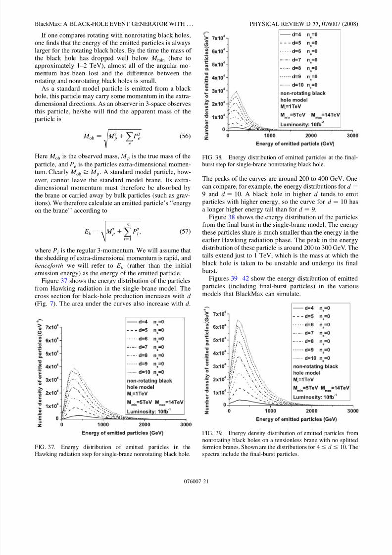
8/3/2019 BlackMax Final
http://slidepdf.com/reader/full/blackmax-final 21/29
If one compares rotating with nonrotating black holes,
one finds that the energy of the emitted particles is always
larger for the rotating black holes. By the time the mass of
the black hole has dropped well below M min (here to
approximately 1–2 TeV), almost all of the angular mo-
mentum has been lost and the difference between the
rotating and nonrotating black holes is small.
As a standard model particle is emitted from a black
hole, this particle may carry some momentum in the extra-dimensional directions. As an observer in 3-space observes
this particle, he/she will find the apparent mass of the
particle is
M ob ��������������������������M 2p �
Xe
P2e
s: (56)
Here M ob is the observed mass, M p is the true mass of the
particle, and Pe is the particles extra-dimensional momen-
tum. Clearly M ob M p. A standard model particle, how-
ever, cannot leave the standard model brane. Its extra-
dimensional momentum must therefore be absorbed by
the brane or carried away by bulk particles (such as grav-itons). We therefore calculate an emitted particle’s ‘‘energyon the brane’’ according to
Eb ���������������������������M 2p �
X3
i�1
P2i
vuut ; (57)
where Pi is the regular 3-momentum. We will assume that
the shedding of extra-dimensional momentum is rapid, and
henceforth we will refer to Eb (rather than the initial
emission energy) as the energy of the emitted particle.
Figure 37 shows the energy distribution of the particles
from Hawking radiation in the single-brane model. Thecross section for black-hole production increases with d(Fig. 7). The area under the curves also increase with d.
The peaks of the curves are around 200 to 400 GeV. One
can compare, for example, the energy distributions for d
�9 and d � 10. A black hole in higher d tends to emitparticles with higher energy, so the curve for d � 10 has
a longer higher energy tail than for d � 9.
Figure 38 shows the energy distribution of the particles
from the final burst in the single-brane model. The energy
these particles share is much smaller than the energy in the
earlier Hawking radiation phase. The peak in the energy
distribution of these particle is around 200 to 300 GeV. The
tails extend just to 1 TeV, which is the mass at which the
black hole is taken to be unstable and undergo its final
burst.
Figures 39–42 show the energy distribution of emitted
particles (including final-burst particles) in the various
models that BlackMax can simulate.
FIG. 37. Energy distribution of emitted particles in the
Hawking radiation step for single-brane nonrotating black hole.
FIG. 38. Energy distribution of emitted particles at the final-
burst step for single-brane nonrotating black hole.
FIG. 39. Energy density distribution of emitted particles from
nonrotating black holes on a tensionless brane with no splitted
fermion branes. Shown are the distributions for 4 d 10. The
spectra include the final-burst particles.
BlackMax: A BLACK-HOLE EVENT GENERATOR WITH . . . PHYSICAL REVIEW D 77, 076007 (2008)
076007-21

8/3/2019 BlackMax Final
http://slidepdf.com/reader/full/blackmax-final 22/29
Figure 39 shows the energy distribution in the single-
brane model. The cross section of black hole increases with
d (Fig. 7). The area under the curves also increases with d.
The peaks of the curves are around 200 GeV to 400. Again
comparing d � 9 and d � 10, a black hole in higher dtends to emit particles with higher energy, so the curve for
d � 10 has a longer high energy tail than for d � 9.
Figure 40 illustrates the split-fermion model. In this
figure, we keep the total number of dimensions d fixed
but change the dimensionality ns of the minibulk. This
affects the spectra of only the gauge boson and scalar
fields, as only their propagation is affected by the mini-
bulk’s dimensionality. (Gravitons propagate in the fullbulk; other standard model particles propagate only on
the brane.) As explained above, these spectra will shift to
higher energies as the number of splitting dimensions is
increased. One can see that the curve in ns � 7 has the
longest high energy tail.
Figure 41 illustrates the brane with tension model. The
energies of the emitted particles shift to lower energy as Bdecreases.
The energy distribution of emitted particles for rotating
black holes (Fig. 42) has the same general characteristics
as the distribution for nonrotating black holes. Angular
momentum causes a black hole to tend to emit higher
energy particles than a nonrotating black hole. The curves
have longer higher energy tails than the nonrotating black
holes.
Figure 43 shows the energy distribution of emitted par-ticles from two-body final-states scenario. The energy of
FIG. 41. Energy distribution of emitted particles for nonrotat-
ing black holes on a nonzero tension brane with B � 1, B � 0:8,
and B � 0:6. The spectra include the final-burst particles.
FIG. 42. Energy distribution of emitted particles for rotating
black holes for 4 d 10.FIG. 40. Energy density distribution of emitted particles from
nonrotating black holes on a tensionless brane with fermion
brane splitting. Shown are the distributions for d � 10 and 0 ns 7. The spectra include the final-burst particles.
FIG. 43. Energy distribution of emitted particles for two-body
final states.
DE-CHANG DAI et al. PHYSICAL REVIEW D 77, 076007 (2008)
076007-22

8/3/2019 BlackMax Final
http://slidepdf.com/reader/full/blackmax-final 23/29
the emitted particles is about the half of the incoming
partons.
In Fig. 44 we show the energy distribution of different
types of particles in the d � 5 single-brane model. The
area of each curve is dependent on the degree of freedom of
each particle and its power spectrum. One can compare the
ratio of the same type of particles. For example, the area of
gluons should be 8 times as large as the area of photons. It
is roughly the same as what the figure shows.
H. Pseudorapidity distributions of the emitted particles
Figures 45– 48 show the pseudorapidity distributions of
the emitted particles for different extra-dimension
scenarios.
Most of black holes are made of two u quarks and have
charge 3=4. For the shown figures, we did not include
FIG. 44. Energy distribution of each particle type in the d � 5single-brane model.
FIG. 46. Pseudorapidity distribution of quarks and antiquarks
for nonrotating black holes on a tensionless brane with and
without the final-burst particles; d � 5.
FIG. 45. Pseudorapidity distribution of charge leptons and
antileptons for nonrotating black holes on a tensionless brane
with and without the final-burst particles; d � 5.
FIG. 47. Pseudorapidity distribution of charged leptons andantileptons for rotating black holes, on a tensionless brane,
with and without the final-burst particles. Here d � 5.
FIG. 48. Pseudorapidity distribution of quarks and antiquarks
for rotating black holes, on a tensionless brane, with and without
the final-burst particles. Here d � 5.
BlackMax: A BLACK-HOLE EVENT GENERATOR WITH . . . PHYSICAL REVIEW D 77, 076007 (2008)
076007-23
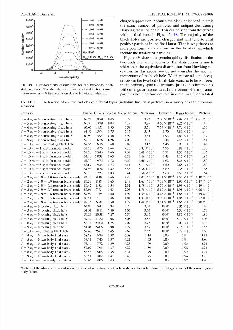
8/3/2019 BlackMax Final
http://slidepdf.com/reader/full/blackmax-final 24/29
charge suppression, because the black holes tend to emit
the same number of particles and antiparticles during
Hawking radiation phase. This can be seen from the curves
without final burst in Figs. 45–48. The majority of the
black holes are positive charged and will tend to emit
positive particles in the final burst. That is why there are
more positrons than electrons for the distributions which
include the final-burst particles.
Figure 49 shows the pseudorapidity distribution in thetwo-body final-state scenario. The distribution is much
wider than the equivalent distribution from Hawking ra-
diation. In this model we do not consider the angular
momentum of the black hole. We therefore take the decay
process in the two-body final-state scenario to be isotropic
in the ordinary spatial directions, just as in other models
without angular momentum. In the center-of-mass frame,
particles are therefore emitted in directions uncorrelated
FIG. 49. Pseudorapidity distribution for the two-body final-
state scenario. The distribution in 2-body final states is much
flatter near � 0 than emission due to Hawking radiation.
TABLE III. The fraction of emitted particles of different types (including final-burst particles) in a variety of extra-dimension
scenarios.
Scenario Quarks Gluons Leptons Gauge bosons Neutrinos Gravitons Higgs bosons Photons
d � 4 ns � 0 nonrotating black hole 68.21 10.79 9.45 5.72 3.87 2:00 10ÿ1 8:99 10ÿ1 8:61 10ÿ1
d � 5 ns � 0 nonrotating black hole 65.37 13.29 9.04 6.12 3.76 4:60 10ÿ1 8:26 10ÿ1 1.13
d � 6 ns � 0 nonrotating black hole 63.63 14.51 8.93 6.58 3.51 7:59 10ÿ1 7:76 10ÿ1 1.30
d � 7 ns � 0 nonrotating black hole 61.25 15.94 8.75 7.17 3.45 1.20 7:89 10ÿ1 1.44
d � 8 ns � 0 nonrotating black hole 60.99 15.94 8.56 6.99 3.35 1.93 7:63 10ÿ1 1.47
d � 9 ns � 0 nonrotating black hole 59.40 16.26 8.26 7.08 3.26 3.48 7:45 10ÿ1 1.51
d � 10 ns � 0 nonrotating black hole 57.56 16.15 7.68 6.82 3.17 6.46 6:97 10ÿ1 1.46
d � 10 ns � 1 split fermions model 61.58 19.76 1.64 7.30 3:83 10ÿ1 6.95 5:88 10ÿ1 1.80
d � 10 ns � 2 split fermions model 61.28 20.40 1.66 7.09 3:49 10ÿ1 6.91 4:56 10ÿ1 1.86
d � 10 ns � 3 split fermions model 62.10 20.33 1.65 6.76 4:46 10ÿ1 6.43 4:15 10ÿ1 1.87
d � 10 ns � 4 split fermions model 62.70 19.76 1.72 6.60 4:66 10ÿ1 6.62 3:28 10ÿ1 1.80
d � 10 ns � 5 split fermions model 63.67 19.34 1.73 6.14 5:17 10ÿ1 6.50 2:65 10ÿ1 1.83
d � 10 ns � 6 split fermions model 64.96 18.24 1.82 5.85 5:56 10ÿ1 6.69 2:35 10ÿ1 1.65
d � 10 ns � 7 split fermions model 66.38 17.23 1.83 5.44 5:50 10ÿ1 6.68 2:51 10ÿ1 1.64d � 2 ns � 2 B � 1:0 tension brane model 84.13 9.39 1.66 2.80 2:02 10ÿ1 9:23 10ÿ1 2:51 10ÿ1 6:30 10ÿ1
d � 2 ns � 2 B � 0:9 tension brane model 85.33 8.88 1.65 2.49 1:63 10ÿ1 7:55 10ÿ1 1:90 10ÿ1 5:47 10ÿ1
d � 2 ns � 2 B � 0:8 tension brane model 86.42 8.32 1.54 2.32 1:79 10ÿ1 5:70 10ÿ1 1:99 10ÿ1 4:49 10ÿ1
d � 2 ns � 2 B � 0:7 tension brane model 87.06 7.93 1.63 2.08 1:75 10ÿ1 5:19 10ÿ1 1:98 10ÿ1 4:00 10ÿ1
d � 2 ns � 2 B � 0:6 tension brane model 87.92 7.39 1.60 1.94 1:59 10ÿ1 4:46 10ÿ1 1:88 10ÿ1 3:59 10ÿ1
d � 2 ns � 2 B � 0:5 tension brane model 88.51 7.11 1.46 1.84 1:33 10ÿ1 3:96 10ÿ1 1:86 10ÿ1 3:67 10ÿ1
d � 2 ns � 2 B � 0:4 tension brane model 89.16 6.58 1.58 1.72 1:49 10ÿ1 3:54 10ÿ1 1:66 10ÿ1 2:90 10ÿ1
d � 4 ns � 0 rotating black hole 64.82 15.41 7.94 6.25 3.50 0.00a 6:06 10ÿ1 1.48
d � 5 ns � 0 rotating black hole 61.38 18.11 7.89 7.06 3.30 0.00a 5:56 10ÿ1 1.70
d � 6 ns � 0 rotating black hole 59.21 20.38 7.27 7.59 3.08 0.00a 5:85 10ÿ1 1.89
d � 7 ns � 0 rotating black hole 57.52 21.82 7.08 8.08 2.87 0.00a 5:77 10ÿ1 2.05
d � 8 ns � 0 rotating black hole 54.41 24.02 6.75 9.09 2.77 0.00a 6:07 10ÿ1 2.36
d � 9 ns � 0 rotating black hole 51.88 24.05 7.98 9.27 3.55 0.00a 7:15 10ÿ1 2.55
d � 10 ns � 0 rotating black hole 52.43 25.67 6.45 9.62 2.52 0.00a
6:79 10ÿ1 2.63d � 4 ns � 0 two-body final states 58.88 16.89 1.38 6.08 11.14 0.00 1.91 3.71
d � 5 ns � 0 two-body final states 57.71 17.46 1.37 6.22 11.53 0.00 1.91 3.80
d � 6 ns � 0 two-body final states 57.16 17.72 1.39 6.27 11.59 0.00 1.93 3.94
d � 7 ns � 0 two-body final states 57.02 17.91 1.37 6.22 11.59 0.00 1.98 3.91
d � 8 ns � 0 two-body final states 56.58 18.08 1.35 6.31 11.79 0.00 1.92 3.97
d � 9 ns � 0 two-body final states 56.51 18.02 1.41 6.40 11.75 0.00 1.96 3.95
d � 10 ns � 0 two-body final states 56.66 18.06 1.43 6.28 11.74 0.00 1.92 3.90
aNote that the absence of gravitons in the case of a rotating black hole is due exclusively to our current ignorance of the correct gray-
body factor.
DE-CHANG DAI et al. PHYSICAL REVIEW D 77, 076007 (2008)
076007-24

8/3/2019 BlackMax Final
http://slidepdf.com/reader/full/blackmax-final 25/29
with the beam direction. Nevertheless, because the thresh-
old energy of the two-body final-state model is much lower
than that of other models, the intermediate state tends to
have a higher velocity down the beam-pipe. The decay
products are therefore emitted with larger pseudorapidity.
In truth, one may expect that the intermediate state of the
two-body final-state scenario has non-negligible angular
momentum. However, since the intermediate state is not a
real black hole, it is unclear exactly what role the angularmomentum of the intermediate state plays.
In the final-state scenario, the momenta of the two
emitted particles are correlated with the initial parton
momenta, and hence the pseudorapidity distribution of
the emitted particles reflects that of the initial partons.
The ratio of the number of events for pseudorapidity
between 0 and 0.5 divided by that for pseudorapidity
between 0.5 and 1 is about 1.1. This is much higher than
the asymptotic QCD value of 0.6, as predicted by [15,106].
If the ratio is found not to equal 0.6, then this would suggestnew physics beyond the standard model.
I. Emitted particle types
Table III shows, for a variety of representative extra-
dimension scenarios, the fraction of emitted particles
which are of each possible type—quarks, gluons,
(charged) leptons, (weak) gauge bosons, neutrinos, grav-
itons, Higgs bosons, and photons. One notable feature is
that the intensity of gravitons relative to other particles
increases with the number of extra dimensions. Note that
the absence of gravitons in the case of a rotating black hole
is not physical, but rather reflects our ignorance of the
correct gray-body factor.
VIII. CONCLUSIONHitherto, black-hole generators for the large-extra-
dimension searches at the LHC have made many simplify-
ing assumptions regarding the model of both our three-
dimensional space and the extra-dimensional space, and
simplifying assumptions regarding the properties of the
black holes that are produced. In this paper we have dis-
cussed a new generator for black holes at the LHC,
BlackMax, which removes many of these assumptions.
With regard to the extra-dimensional model it allows for
brane tension, and brane splitting. With regard to the black
hole, it allows for black-hole rotation, charge (both elec-
tromagnetic and color), and bulk recoil. It also introduces
the possibility of a two-body final state that is not a black
hole.
Although BlackMax represents a major step forward,
there remain important deficiencies that will need to be
addressed in the future. BlackMax continues to insist on a
flat geometry for the bulk space, whereas there is consid-
erable interest in a warped geometry [2] or in a compacthyperbolic geometry [3]. While BlackMax allows for
black-hole rotation, the absence of either an analytic or a
numerical gray-body factor for the graviton in more than
three space dimensions for rotating black holes is a serious
shortcoming that can be expected to materially change the
signature of black-hole decay for rotating black holes.
Other issues include how to properly account for the likely
suppression of decays that cause a black hole to acquire
very ‘‘large’’ color, charge, or angular momentum (as
opposed to the somewhat contrived phenomenological ap-
proach currently taken). These are but a few of the funda-mental issues that remain to be clarified.
Despite these (and no doubt other) shortcomings, weexpect that BlackMax will allow for a much improved
understanding of the signatures of black holes at the
LHC. Work in progress focuses on using BlackMax to
explore the consequences for the ATLAS experiment of
more realistic black-hole and extra-dimension models.
ACKNOWLEDGMENTS
We thank Nicholas Brett for discussions in the early
stages of this paper. We thank Daisuke Ida, Kin-ya Oda,
and Seong Chan Park for providing some of the spectra of rotating black holes. D. C. D., D.S., and G.D. S. thank
Oxford’s Atlas group for its hospitality at various stages
of this project. D.C. D., D.S., and G. D.S. have been
supported in part by a grant from the U.S. DOE; G. D. S.
was supported in part by the John Simon Guggenheim
Memorial Foundation and by Oxford’s Beecroft Institute
for Particle Astrophysics and Cosmology.
APPENDIX: PARTICLE EMISSION SPECTRA
Nowadays gray-body factors can be found in many
papers. We collect the relevant papers in Table I. We follow
these papers to calculate energy power spectra in ourdatabase except for the split-fermions model (although
we independently confirm the results as well). We perform
an original calculation of the spectra of gauge bosons and
scalar fields in the split-fermions model as a function of the
FIG. 50. Spectra of scalar fields in d � 5 space.
BlackMax: A BLACK-HOLE EVENT GENERATOR WITH . . . PHYSICAL REVIEW D 77, 076007 (2008)
076007-25

8/3/2019 BlackMax Final
http://slidepdf.com/reader/full/blackmax-final 26/29
FIG. 51. Spectra of scalar fields in d � 6 space.
FIG. 53. Spectra of scalar fields in d � 8 space.
FIG. 52. Spectra of scalar fields in d � 7 space.
FIG. 54. Spectra of scalar fields in d � 9 space.
FIG. 56. Spectra of gauge bosons in d � 5 space.
FIG. 55. Spectra of scalar fields in d � 10 space.
DE-CHANG DAI et al. PHYSICAL REVIEW D 77, 076007 (2008)
076007-26

8/3/2019 BlackMax Final
http://slidepdf.com/reader/full/blackmax-final 27/29
number of dimensions ns in which the fermion branes are
split. These are shown in Figs. 50–61.
Anyone who has a better spectrum can upgrade our
database. For example, we only calculate the spectra up
to the l � 9 mode.
FIG. 57. Spectra of gauge bosons in d � 6 space.
FIG. 58. Spectra of gauge bosons in d � 7 space.
FIG. 59. Spectra of gauge bosons in d � 8 space.
FIG. 60. Spectra of gauge bosons in d � 9 space.
FIG. 61. Spectra of gauge bosons in d � 10 space.
BlackMax: A BLACK-HOLE EVENT GENERATOR WITH . . . PHYSICAL REVIEW D 77, 076007 (2008)
076007-27
8/3/2019 BlackMax Final
http://slidepdf.com/reader/full/blackmax-final 28/29
[1] Nima Arkani-Hamed, Savas Dimopoulos, and G.R. Dvali,
Phys. Rev. D 59, 086004 (1999); Ignatios Antoniadis,
Nima Arkani-Hamed, Savas Dimopoulos, and G.R.
Dvali, Phys. Lett. B 436, 257 (1998); Nima Arkani-Hamed, Savas Dimopoulos, and G. R. Dvali, Phys. Lett.
B 429, 263 (1998).
[2] Lisa Randall and Raman Sundrum, Phys. Rev. Lett. 83,
4690 (1999).
[3] N. Kaloper, J. March-Russell, G. D. Starkman, and M.
Trodden, Phys. Rev. Lett. 85, 928 (2000); G.D. Starkman,
D. Stojkovic, and M. Trodden, Phys. Rev. Lett. 87, 231303
(2001); Phys. Rev. D 63, 103511 (2001).
[4] I. Antoniadis, Phys. Lett. B 246, 377 (1990); K.R. Dienes,
E. Dudas, and T. Gherghetta, Phys. Lett. B 436, 55 (1998).
[5] T. Banks and W. Fischler, arXiv:hep-th/9906038; S.
Dimopoulos and G. Landsberg, Phys. Rev. Lett. 87,
161602 (2001); S. B. Giddings and S. Thomas, Phys.
Rev. D 65, 056010 (2002).[6] K.S. Thorne, in Magic Without Magic, edited by JR.
Klauder (Freeman, San Francisco, 1972), pp. 231–258;
D. Ida and K.-i. Nakao, Phys. Rev. D 66, 064026 (2002);
H. Yoshino and Y. Nambu, Phys. Rev. D 66, 065004
(2002).
[7] T. Vachaspati, D. Stojkovic, and L.M. Krauss, Phys. Rev.
D 76, 024005 (2007); T. Vachaspati and D. Stojkovic,
arXiv:gr-qc/0701096.
[8] TRUENOIR: Savas Dimopoulos and Greg L. Landsberg,
Phys. Rev. Lett. 87, 161602 (2001); CHARYBDIS: C. M.
Harris, P. Richardson, and B. R. Webber, J. High Energy
Phys. 08 (2003) 033; Catfish: M. Cavaglia, R. Godang, L.
Cremaldi, and D. Summers, arXiv:hep-ph/0609001.
[9] D. C. Dai, G. D. Starkman, and D. Stojkovic, Phys. Rev. D73, 104037 (2006); D. Stojkovic, G. D. Starkman, and
D. C. Dai, Phys. Rev. Lett. 96, 041303 (2006).
[10] D. Stojkovic, F. C. Adams, and G. D. Starkman, Int. J.
Mod. Phys. D 14, 2293 (2005); C. Bambi, A. D. Dolgov,
and K. Freese, Nucl. Phys. B763, 91 (2007); J. Cosmol.
Astropart. Phys. 04 (2007) 005.
[11] N. Arkani-Hamed and M. Schmaltz, Phys. Rev. D 61,
033005 (2000).
[12] Ya. B. Zel’dovich, Pis’ma Zh. Eksp. Teor. Fiz. 12, 443
(1970); JETP Lett. 14, 180 (1971); Sov. Phys. JETP 35,
1085 (1972); C. W. Misner, Phys. Rev. Lett. 28, 994
(1972); V. P. Frolov and D. Stojkovic, Phys. Rev. D 67,
084004 (2003); 68, 064011 (2003).
[13] Nemanja Kaloper and Derrick Kiley, J. High Energy Phys.03 (2006) 077.
[14] De-Chang Dai, Nemanja Kaloper, Glenn D. Starkman, and
Dejan Stojkovic, Phys. Rev. D 75, 024043 (2007).
[15] Patrick Meade and Lisa Randall, arXiv:0708.3017.
[16] Vitor Cardoso, Marco Cavaglia, and Leonardo Gualtieri, J.
High Energy Phys. 02 (2006) 021.
[17] Christopher Michael Harris, Ph.D. thesis, Christ’s College,
University of Cambridge [arXiv:hep-ph/0502005].
[18] Chris M. Harris and Panagiota Kanti, J. High Energy Phys.
10 (2003) 014.
[19] G. Duffy, C. Harris, P. Kanti, and E. Winstanley, J. High
Energy Phys. 09 (2005) 049.
[20] C. M. Harris and P. Kanti, Phys. Lett. B 633, 106 (2006).[21] M. Casals, P. Kanti, and E. Winstanley, J. High Energy
Phys. 02 (2006) 051.
[22] M. Casals, S.R. Dolan, P. Kanti, and E. Winstanley, J.
High Energy Phys. 03 (2007) 019.
[23] Daisuke Ida, Kin-ya Oda, and Seong Chan Park, Phys.
Rev. D 73, 124022 (2006).
[24] S. Creek, O. Efthimiou, P. Kanti, and K. Tamvakis, Phys.
Rev. D 75, 084043 (2007); Phys. Lett. B 594, 363 (2004);
T. Harmark, J. Natario, and R. Schiappa, arXiv:0708.0017.
[25] D. Stojkovic, Phys. Rev. Lett. 94, 011603 (2005).
[26] Luis A. Anchordoqui, Jonathan L. Feng, Haim Goldberg,
and Alfred D. Shapere, Phys. Lett. B 594, 363 (2004).
[27] V. Frolov and D. Stojkovic, Phys. Rev. Lett. 89, 151302
(2002); Phys. Rev. D 66, 084002 (2002); D. Stojkovic,Phys. Rev. Lett. 94, 011603 (2005).
[28] D. Stojkovic, J. High Energy Phys. 09 (2004) 061.
[29] D. Ida, K. Oda, and S. C. Park, Phys. Rev. D 67, 064025
(2003); 69, 049901(E) (2004).
[30] A. Flachi, O. Pujolas, M. Sasaki, and T. Tanaka,
arXiv:hep-th/0601174; A. Flachi and T. Tanaka, Phys.
Rev. Lett. 95, 161302 (2005).
[31] T.G. Rizzo, Classical Quantum Gravity 23, 4263 (2006);
arXiv:hep-ph/0510420; J. High Energy Phys. 01 (2005)
028.
[32] D. K. Park, Classical Quantum Gravity 23, 4101 (2006);
Phys. Lett. B 633, 613 (2006).
[33] M. Casals, P. Kanti, and E. Winstanley, J. High Energy
Phys. 02 (2006) 051.[34] R. da Rocha and C.H. Coimbra-Araujo, J. Cosmol.
Astropart. Phys. 12 (2005) 009.
[35] A. S. Cornell, W. Naylor, and M. Sasaki, J. High Energy
Phys. 02 (2006) 012;
[36] J. Grain, A. Barrau, and P. Kanti, Phys. Rev. D 72, 104016
(2005).
[37] H. Yoshino, T. Shiromizu, and M. Shibata, Phys. Rev. D
72, 084020 (2005).
[38] G. Duffy, C. Harris, P. Kanti, and E. Winstanley, J. High
Energy Phys. 09 (2005) 049.
[39] E. Jung and D. K. Park, Nucl. Phys. B731, 171 (2005).
[40] L. Lonnblad, M. Sjodahl, and T. Akesson, J. High Energy
Phys. 09 (2005) 019.
[41] J. I. Illana, M. Masip, and D. Meloni, Phys. Rev. D 72,024003 (2005).
[42] E. Jung, S. Kim, and D. K. Park, Phys. Lett. B 619, 347
(2005); 614, 78 (2005).
[43] H. Yoshino and V. S. Rychkov, Phys. Rev. D 71, 104028
(2005).
[44] A. S. Majumdar and N. Mukherjee, Int. J. Mod. Phys. D
14, 1095 (2005); Mod. Phys. Lett. A 20, 2487 (2005).
[45] A. Perez-Lorenzana, arXiv:hep-ph/0503177.
[46] D. Ida, K. Oda, and S. C. Park, Phys. Rev. D 71, 124039
DE-CHANG DAI et al. PHYSICAL REVIEW D 77, 076007 (2008)
076007-28
8/3/2019 BlackMax Final
http://slidepdf.com/reader/full/blackmax-final 29/29
(2005); Phys. Rev. D 73, 124022 (2006).
[47] V. P. Frolov, D. V. Fursaev, and D. Stojkovic, Classical
Quantum Gravity 21, 3483 (2004); J. High Energy Phys.
06 (2004) 057.
[48] A. N. Aliev and A. E. Gumrukcuoglu, Phys. Rev. D 71,
104027 (2005); A. N. Aliev, Mod. Phys. Lett. A 21, 751
(2006); A. N. Aliev and V. P. Frolov, Phys. Rev. D 69,
084022 (2004).
[49] P. Kanti, J. Grain, and A. Barrau, Phys. Rev. D 71, 104002
(2005); P. Kanti and K. Tamvakis, Phys. Rev. D 65,084010 (2002); P. Kanti and J. March-Russell, Phys.
Rev. D 67, 104019 (2003); P. Kanti, Int. J. Mod. Phys.
A 19, 4899 (2004).
[50] H. Yoshino and Y. Nambu, Phys. Rev. D 70, 084036
(2004).
[51] E. F. Eiroa, Braz. J. Phys. 35, 1113 (2005); Phys. Rev. D
71, 083010 (2005).
[52] P. S. Apostolopoulos, N. Brouzakis, E. N. Saridakis, and
N. Tetradis, Phys. Rev. D 72, 044013 (2005).
[53] S. Creek, O. Efthimiou, P. Kanti, and K. Tamvakis, Phys.
Lett. B 635, 39 (2006).
[54] D. Stojkovic, Phys. Rev. D 67, 045012 (2003).
[55] E. Berti, V. Cardoso, and M. Casals, Phys. Rev. D 73,
024013 (2006).[56] M. Vasudevan and K.A. Stevens, Phys. Rev. D 72, 124008
(2005).
[57] B.M. N. Carter and I.P. Neupane, Phys. Rev. D 72,
043534 (2005).
[58] L. Lonnblad, M. Sjodahl, and T. Akesson, J. High Energy
Phys. 09 (2005) 019.
[59] V. Frolov, M. Snajdr, and D. Stojkovic, Phys. Rev. D 68,
044002 (2003).
[60] M. Nozawa and K. Maeda, Phys. Rev. D 71, 084028
(2005).
[61] C. M. Harris, arXiv:hep-ph/0502005.
[62] Y. Morisawa and D. Ida, Phys. Rev. D 71, 044022 (2005).
[63] V. Cardoso, O.J. C. Dias, and J.P. S. Lemos, Phys. Rev. D
67, 064026 (2003); V. Cardoso, O.J.C. Dias, J.L.Hovdebo, and R. C. Myers, Phys. Rev. D 73, 064031
(2006).
[64] A. Cafarella, C. Coriano, and T.N. Tomaras, AIP Conf.
Proc. 756, 457 (2005).
[65] A. Chamblin, F. Cooper, and G. C. Nayak, Phys. Rev. D
70, 075018 (2004); 69, 065010 (2004).
[66] D. Ida, Y. Uchida, and Y. Morisawa, Phys. Rev. D 67,
084019 (2003).
[67] E. J. Ahn and M. Cavaglia, Phys. Rev. D 73, 042002
(2006).
[68] M. Cavaglia and S. Das, Classical Quantum Gravity 21,
4511 (2004); M. Cavaglia, S. Das, and R. Maartens,
Classical Quantum Gravity 20, L205 (2003).
[69] V. Cardoso, M. Cavaglia, and L. Gualtieri, J. High EnergyPhys. 02 (2006) 021.
[70] L. A. Anchordoqui, J. L. Feng, H. Goldberg, and A. D.
Shapere, Phys. Lett. B 594, 363 (2004); L. Anchordoqui
and H. Goldberg, Phys. Rev. D 67, 064010 (2003); L.
Anchordoqui, T. Han, D. Hooper, and S. Sarkar, Astropart.
Phys. 25, 14 (2006).
[71] A. Casanova and E. Spallucci, Classical Quantum Gravity
23, R45 (2006).
[72] J. E. Aman and N. Pidokrajt, Phys. Rev. D 73, 024017
(2006).
[73] U. Harbach and M. Bleicher, arXiv:hep-ph/0601121.
[74] B. Koch, M. Bleicher, and S. Hossenfelder, J. High Energy
Phys. 10 (2005) 053; S. Hossenfelder, Phys. Lett. B 598,
92 (2004).
[75] M. Fairbairn, arXiv:hep-ph/0509191.
[76] G.L. Alberghi, R. Casadio, D. Galli, D. Gregori, A.
Tronconi, and V. Vagnoni, arXiv:hep-ph/0601243.
[77] P. Davis, Classical Quantum Gravity 23, 3607 (2006); P.
Krtous and J. Podolsky, Classical Quantum Gravity 23,1603 (2006).
[78] K. A. Bronnikov, S. A. Kononogov, and V. N. Melnikov,
Gen. Relativ. Gravit. 38, 1215 (2006).
[79] B. Koch, M. Bleicher, and H. Stoecker, J. Phys. G 34,
S535 (2007).
[80] S. Chen, B. Wang, and R.K. Su, Phys. Lett. B 647, 282
(2007).
[81] H. T. Cho, A.S. Cornell, J. Doukas, and W. Naylor, Phys.
Rev. D 75, 104005 (2007).
[82] L.h. Liu, B. Wang, and G. h. Yang, Phys. Rev. D 76,
064014 (2007).
[83] B. Koch, arXiv:0707.4644.
[84] H. Stoecker, J. Phys. G 32, S429 (2006).
[85] B. Betz, M. Bleicher, U. Harbach, T. Humanic, B. Koch,and H. Stoecker, J. Phys. G 32, S429 (2006).
[86] A. N. Aliev, Phys. Rev. D 75, 084041 (2007).
[87] T. G. Rizzo, Phys. Lett. B 647, 43 (2007).
[88] D. M. Gingrich, Int. J. Mod. Phys. A 21, 6653 (2006); J.
High Energy Phys. 11 (2007) 064.
[89] E. Abdalla, C.B. M. Chirenti, and A. Saa, J. High Energy
Phys. 10 (2007) 086.
[90] G. L. Landsberg, J. Phys. G 32, R337 (2006).
[91] H. Yoshino and R.B. Mann, Phys. Rev. D 74, 044003
(2006).
[92] Y. i. Takamizu, H. Kudoh, and K. i. Maeda, Phys. Rev. D
75, 061304 (2007).
[93] R. da Rocha and C.H. Coimbra-Araujo, Phys. Rev. D 74,
055006 (2006).[94] S. Creek, R. Gregory, P. Kanti, and B. Mistry, Classical
Quantum Gravity 23, 6633 (2006).
[95] A. Perez-Lorenzana, J. Phys. Conf. Ser. 18, 224 (2005).
[96] A. Lopez-Ortega, Gen. Relativ. Gravit. 39, 1011 (2007).
[97] H. K. Kunduri, J. Lucietti, and H. S. Reall, Phys. Rev. D
74, 084021 (2006).
[98] H. T. Cho, A.S. Cornell, J. Doukas, and W. Naylor, Phys.
Rev. D 75, 104005 (2007).
[99] S. B. Giddings, AIP Conf. Proc. 957, 69 (2007).
[100] S. Creek, O. Efthimiou, P. Kanti, and K. Tamvakis, Phys.
Lett. B 656, 102 (2007).
[101] S. Chen, B. Wang, and R.K. Su, Phys. Rev. D 77, 024039
(2008).
[102] A. Barrau, J. Grain, and C. Weydert, Phys. Rev. D 76,087503 (2007).
[103] U. A. al-Binni and G. Siopsis, Phys. Rev. D76, 104031
(2007).
[104] D. Kiley, Phys. Rev. D 76, 126002 (2007).
[105] J. Pumplin et al., J. High Energy Phys. 07 (2002) 012; D.
Stump et al., J. High Energy Phys. 10 (2003) 046.
[106] B. Abbott et al. (D0 Collaboration), Phys. Rev. Lett. 82,
2457 (1999).
BlackMax: A BLACK-HOLE EVENT GENERATOR WITH . . . PHYSICAL REVIEW D 77, 076007 (2008)