blasting design using fracture toughness and image ... fragmentation using the kuz-ram model, an...
TRANSCRIPT

Blasting Design Using Fracture Toughness and Image Analysis
of the Bench Face and Muckpile
Kwangmin Kim
Thesis submitted to the Faculty of the Virginia Polytechnic Institute and State University in partial fulfillment of the requirements for the degree of
Master of Science
In
Mining and Minerals Engineering
Committee Members:
Dr. Erik C. Westman, Chair
Dr. Mario G. Karfakis Dr. Tom Novak
July 21, 2006 Blacksburg, Virginia
Keywords: Fracture toughness, Blasting, Image analysis

Blasting Design Using Fracture Toughness and Image Analysis of the Bench Face and Muckpile
Kwangmin Kim
Abstract
Few studies of blasting exist because of difficulties in obtaining reliable fragmentation data
or even obtaining consistent blasting results. Many researchers have attempted to predict
blast fragmentation using the Kuz-Ram model, an empirical fragmentation model suggested
by Cunningham.
The purpose of this study is to develop an empirical model to relate specific explosives
energy (ESE) to blasting fragmentation reduction ratio (RR) and rock fracture toughness
(KIC).
The reduction ratio was obtained by analyzing the bench face block size distribution and
the muck fragment size distribution using image analysis. The fracture toughness was
determined using the Edge Notched Disk Wedge Splitting test.
Blasting data from twelve (12) blasts at four (4) different quarries were analyzed. Based on
this data set, an empirical relationship, ESE=11.7 RR801.202 KIC
4.14 has been developed. Using
this relationship, based on the predicted blasting energy input for a desired eighty-percent
passing (P80) muckpile fragment size the burden and spacing may be determined.

ACKNOWLEDGEMENT
First and foremost I would like to express my sincere appreciation to my advisor Dr. Erik C.
Westman and co-advisor Dr. Mario G. Karfakis for their guidance, and encouragement. In
spite of their busy schedule, their participation was precious. Their suggestion on this work
was valuable and helpful. I would also like to thank to my committee member, Dr. Tom
Novak.
My parents Youngduck Kim, and Guinam Bae, and my wife, Yundeok Kim, their support,
trust, and sacrifice made a big portion of this thesis.
iii

TABLE OF CONTENTS
Page
Abstract ............................................................................................................................ⅱ
Acknowledgement............................................................................................................ⅲ
Table of Contents.............................................................................................................ⅳ
List of Figures....................................................................................................................ⅶ
List of Tables ..................................................................................................................... xi
Chapter 1 - Introduction...................................................................................................1
1.1 Statement of the Problem ...........................................................................................1
1.2 Proposed Solution....................................................................................................2
Chapter 2 – Literature review ..........................................................................................4
2.1 Image analysis .........................................................................................................4
The Reduction Ratio (RR) in blasting............................................................................4
2.1.1 Image analysis programs ....................................................................................5
The IPACS system........................................................................................................5
TUCIPS system ............................................................................................................5
FRAGSCAN .................................................................................................................6
WipFrag system ...........................................................................................................6
SPLIT system ...............................................................................................................6
2.1.2 The errors associated with image processing systems........................................7
2.2 Fracture toughness...................................................................................................8
Single Particle Breakage Testing ................................................................................10
2.3 Blasting fragmentation prediction .........................................................................12
2.3.1 Kuz-Ram model................................................................................................12
The mean size of the fragments formed by blasted rock............................................13
Cunningham ..............................................................................................................14
Limitation of the Kuz-Ram.........................................................................................16
2.3.2 Larsson’s model................................................................................................16
iv

2.3.3 The SVEDEFO (Swedish Detonic Research Foundation) model ....................17
Chapter 3 – Experiment..................................................................................................19
3.1 Image sampling and analysis from a quarry blast .................................................19
3.1.1 Image sampling ................................................................................................20
The image sampling on a bench face ........................................................................21
The image sampling from a muckpile after blasting .................................................22
3.1.2 Image analysis using SPLIT.............................................................................23
The image analysis on a bench face ..........................................................................24
The image analysis on a muckpile.............................................................................25
The size distribution curves from a bench face and a muckpile ................................27
F50 and the mean in-situ block size ..........................................................................28
3.2 Calculation of KIC..................................................................................................29
3.3 Blasting specific explosives energy.......................................................................31
3.4 The main issues in SPLIT for the research............................................................32
An average size and P50 in SPLIT ..............................................................................32
Larger or smaller image..............................................................................................32
Fines ............................................................................................................................33
The selection of the fines percent adjustment in a muckpile .......................................33
Chapter 4 – Data analysis ...............................................................................................34
4.1 The equation model ...............................................................................................35
4.1.1 Specific explosives energy, KIC and RR80 ........................................................36
RR50 and RR80 ............................................................................................................38
4.1.2 Specific explosives energy, KIC and RR20 ...........................................................39
4.1.3 P50 and P80.........................................................................................................42
Chapter 5 – Discussion of results ...................................................................................46
5.1 Improvements revealed by the research ................................................................46
5.2 The bench face structure and the blasting design for desired consistent results ...48
5.3 P80 for the optimal blasting in a quarry ................................................................48
5.4 Generalized blasting model ...................................................................................49
v

5.5 Application for the simulation model....................................................................50
Chapter 6 – Conclusion and future work ......................................................................53
6.1 Research summary.................................................................................................53
6.2 Conclusion.............................................................................................................56
Application ..................................................................................................................57
6.3 Limitation in the research and future work ...........................................................59
Muckpile image sampling ............................................................................................59
Data .............................................................................................................................59
P80...............................................................................................................................59
P50 and P80 ................................................................................................................60
P20 and fines ...............................................................................................................60
References ........................................................................................................................61
Appendix A. Image Analysis of the Bench Face ...........................................................65
Appendix B. Image Analysis of the Muckpile ...............................................................90
Appendix C. Rock Tests (Brazillian, Tilt, and KIC Test) ...........................................115
Appendix D. Summarized Blasting Pattern and ESE..................................................124
vi

LIST OF FIGURES
Figure 1.1 Blasting in Pittsboro...........................................................................................2
Figure 2.1 The Reduction Ratio in a crusher.......................................................................4
Figure 2.2 Image of the muckpile and delineated image using the Split software..............8
Figure 3.1 The released rock from in-situ block of the bench in Warrenton, VA.............19
Figure 3.2 The bench face image in Pittsboro ...................................................................20
Figure 3.3 The bench face image from Bosung quarry .....................................................21
Figure 3.4 The muckpile image from Bosung quarry .......................................................22
Figure 3.5 The analyzed bench face image of Bosung quarry in SPLIT...........................25
Figure 3.6 The muckpile image and analyzed image in SPLIT ........................................26
Figure 3.7 The size distribution curves from the bench face and muckpile......................27
Figure 3.8 Test set-up for END wedge test .......................................................................29
Figure 4.1 The accuracy between predicted ESE and ESE with given RR80 and KIC ..........37
Figure 4.2 Predicted ESE for RR80 and given KIC ..............................................................38
Figure 4.3 RR50 and RR80 ..................................................................................................39
Figure 4.4 Accuracy between predicted ESE and ESE with given RR20 and KIC ................41
Figure 4.5 Liberated versus broken rock in the Pittsboro blast .........................................41
Figure 4.6 The accuracy between predicted P50 and P50.................................................45
Figure 5.1 Simulation using Visual Basic.Net program....................................................52
Figure A.1 Bosung1, the bench face image.......................................................................66
Figure A.2 Bosung1, the analyzed image..........................................................................66
Figure A.3 Bosung1, the size distribution of the bench face.............................................67
Figure A.4 Bosung2, the bench face image.......................................................................68
Figure A.5 Bosung2, the analyzed image..........................................................................68
Figure A.6 Bosung2, the size distribution of the bench face.............................................69
Figure A.7 Bosung3, the bench face image.......................................................................70
Figure A.8 Bosung3, the analyzed image..........................................................................70
Figure A.9 Bosung3, the size distribution of the bench face.............................................71
vii

Figure A.10 Bosung4, the bench face image.....................................................................72
Figure A.11 Bosung4, the analyzed image........................................................................72
Figure A.12 Bosung4, the size distribution of the bench face...........................................73
Figure A.13 Bosung5, the bench face image.....................................................................74
Figure A.14 Bosung5, the analyzed image........................................................................74
Figure A.15 Bosung5, the size distribution of the bench face...........................................75
Figure A.16 Pittsboro, the bench face image ....................................................................76
Figure A.17 Pittsboro, the analyzed image .......................................................................76
Figure A.18 Pittsboro, the size distribution of the bench face ..........................................77
Figure A.19 Boxley, the bench face image .......................................................................78
Figure A.20 Boxley, the analyzed image ..........................................................................78
Figure A.21 Boxley, the size distribution of the bench face .............................................79
Figure A.22 Sanyang1, the bench face image ...................................................................80
Figure A.23 Sanyang1, the analyzed image ......................................................................80
Figure A.24 Sanyang1, the size distribution of the bench face .........................................81
Figure A.25 Sanyang2, the bench face image ...................................................................82
Figure A.26 Sanyang2, the analyzed image ......................................................................82
Figure A.27 Sanyang2, the size distribution of the bench face .........................................83
Figure A.28 Sanyang3, the bench face image ...................................................................84
Figure A.29 Sanyang3, the analyzed image ......................................................................84
Figure A.30 Sanyang3, the size distribution of the bench face .........................................85
Figure A.31 Sanyang4, the bench face image ...................................................................86
Figure A.32 Sanyang4, the analyzed image ......................................................................86
Figure A.33 Sanyang4, the size distribution of the bench face .........................................87
Figure A.34 Sanyang5, the bench face image ...................................................................88
Figure A.35 Sanyang5, the analyzed image ......................................................................88
Figure A.36 Sanyang5, the size distribution of the bench face .........................................89
Figure B.1 Bosung1, the muckpile image .........................................................................91
Figure B.2 Bosung1, the analyzed image ..........................................................................91
viii

Figure B.3 Bosung1, the size distribution of the muckpile ...............................................92
Figure B.4 Bosung2, the muckpile image .........................................................................93
Figure B.5 Bosung2, the analyzed image ..........................................................................93
Figure B.6 Bosung2, the size distribution of the muckpile ...............................................94
Figure B.7 Bosung3, the muckpile image .........................................................................95
Figure B.8 Bosung3, the analyzed image ..........................................................................95
Figure B.9 Bosung3, the size distribution of the muckpile ...............................................96
Figure B.10 Bosung4, the muckpile image .......................................................................97
Figure B.11 Bosung4, the analyzed image ........................................................................97
Figure B.12 Bosung4, the size distribution of the muckpile .............................................98
Figure B.13 Bosung5, the muckpile image .......................................................................99
Figure B.14 Bosung5, the analyzed image ........................................................................99
Figure B.15 Bosung5, the size distribution of the muckpile ...........................................100
Figure B.16 Pittsboro, the muckpile image .....................................................................101
Figure B.17 Pittsboro, the analyzed image......................................................................101
Figure B.18 Pittsboro, the size distribution of the muckpile ...........................................102
Figure B.19 Boxley, the muckpile image........................................................................103
Figure B.20 Boxley, the analyzed image.........................................................................103
Figure B.21 Boxley, the size distribution of the muckpile..............................................104
Figure B.22 Sanyang1, the muckpile image....................................................................105
Figure B.23 Sanyang1, the analyzed image ....................................................................105
Figure B.24 Sanyang1, the size distribution of the muckpile..........................................106
Figure B.25 Sanyang2, the muckpile image....................................................................107
Figure B.26 Sanyang2, the analyzed image ....................................................................107
Figure B.27 Sanyang2, the size distribution of the muckpile..........................................108
Figure B.28 Sanyang3, the muckpile image....................................................................109
Figure B.29 Sanyang3, the analyzed image ....................................................................109
Figure B.30 Sanyang3, the size distribution of the muckpile..........................................110
Figure B.31 Sanyang4, the muckpile image....................................................................111
ix

Figure B.32 Sanyang4, the analyzed image ....................................................................111
Figure B.33 Sanyang4, the size distribution of the muckpile..........................................112
Figure B.34 Sanyang5, the muckpile image....................................................................113
Figure B.35 Sanyang5, the analyzed image ....................................................................113
Figure B.36 Sanyang5, the size distribution of the muckpile..........................................114
x
LIST OF TABLES
Table 3.1 The data from the size distribution curve of the bench face and muckpile.......28
Table 3.2 The data from the bench face and the manually measured block size ..............28
Table 3.3 Values ofφ andµ of four quarries rock............................................................30
Table 3.4 Fracture toughness, KIC, tensile strength, tσ , and specific gravity...................31
Table 3.5 Blasting pattern and ESE in Pittsboro blasting ...................................................32
Table 4.1 The obtained data of blasting ............................................................................35
Table 4.2 ESE with given KIC and RR80 .............................................................................36
Table 4.3 ESE with given KIC and RR20 .............................................................................40
Table 4.4 P50 and P80 in Bosung and Sanyang................................................................44
Table 6.1 Fracture toughness, KIC, and Tensile strength, tσ ............................................53
Table 6.2 Blasting data from image analysis, END test, and the blasting pattern ............54
Table C.1 Bosung, Mode I fracture toughness, KIC ........................................................116
Table C.2 Bosung, Size check for KIC validity................................................................116
Table C.3 Bosung, Brazilian Test....................................................................................117
Table C.4 Bosung, Tilt test..............................................................................................117
Table C.5 Sanyang, Mode I fracture toughness, KIC .......................................................118
Table C.6 Sanyang, Size check for KIC validity ..............................................................118
Table C.7 Sanyang, Brazilian Test ..................................................................................119
Table C.8 Sanyang, Tilt test ............................................................................................119
Table C.9 Boxley, Mode I fracture toughness, KIC .........................................................120
Table C.10 Boxley, Size check for KIC validity ..............................................................120
Table C.11 Boxley, Brazilian Test ..................................................................................121
Table C.12 Boxley, Tilt test ............................................................................................121
Table C.13 Pittsboro, Mode I fracture toughness, KIC ....................................................122
Table C.14 Pittsboro, Size check for KIC validity ...........................................................122
Table C.15 Pittsboro, Brazilian Test ...............................................................................123
xi

Table C.16 Pittsboro, Tilt test..........................................................................................123
Table D.1 Summarized blasting pattern and ESE.............................................................125
xii

Chapter 1 Introduction
1.1 Statement of the Problem
The United States National Materials Advisory Board estimates that improving the energy
efficiency of comminution processes using a practical approach could result in energy
savings of over twenty (20) billion kilowatt-hours per year. Practical savings in the
comminution process, especially blasting, is one of the most important steps (Adel, 2004).
Few studies of blasting exist because of the difficulty in obtaining reliable fragmentation
data, and getting consistent results is difficult. Furthermore, although blasting engineers
differ with regards to desired results, all blasting designs rely on the experience of these
engineers. Excessive fines or oversized fragments are examples of what to avoid. Blasting
has historically been regarded as a stand-alone operation and is usually reported as a single
cost in most analyses.
Blasting engineers widely use the Kuz-Ram model to predict the rock size distribution
arising from blasting. Many researchers have attempted to predict blast fragmentation using
the Kuz-Ram model, which is based on empirical studies of fragmentation.
The model has two primary parameters: the characteristic size, derived from blasting
parameters using the model of Kuznetsov (Kuznetsov, 1973), and a uniformity index, based
on geometric parameters of the drilling and blast design. The size distribution curve is
determined by these two parameters. However, this original Kuz-Ram fragmentation model
is limited in its application and erroneously assumes a fifty percent (50%) passing size as
the average adjusted size in the Rosin-Rammler model (Spathis, 2004 and Chung &
Katsabanis, 2000). In addition, even though the fracturing of rock, as well as of other
materials, is usually due to tensile failure, no current blasting model considers tensile
1

strength. For example, the Kuz-Ram model considers the Uniaxial Compressive Strength
(UCS) and the Young’s Modulus (E).
Figure 1.1 Blasting in Pittsboro
In-situ block size is an important aspect of any blasting model and design because many
pieces of blasted rock are released from the in-situ block, as shown in Figure 1.1. Currently
in-situ block size is still obtained by manually estimating the bench face because there is no
instrument for measuring a whole bench face to obtain easily and cheaply an in-situ block
size.
1.2 Proposed Solution
The purpose of this study is to develop a new empirical model in order to obtain the proper
burden and spacing for target fragment size, P80 (the desired eighty percent [80%] passing
size) in the muckpile and to predict a size distribution curve from the muckpile after a
bench blasting.
A blasting fragmentation model of the same form as the model proposed by Donovan’s for
energy prediction in the comminution is considered, the proposed model is as follow.
c
SE aE ICb K RR =
2

Where:
- ESE is specific explosives energy (wh/ton).
- RR is the reduction ration based on % passing.
- KIC is Mode I fracture toughness value (Mpa*m1/2).
- a,b, and c are constant.
The blasting reduction ratio (RR) is obtained by determining the in-situ block size on the
bench face and the blasting muckpile fragment size using image analysis. The fracture
toughness, KIC, is determined using the Edge Notched Disk Wedge Splitting test (END) on
samples prepared from post blast rock blocks.
3

Chapter 2 Literature Review
The proposed equation, , is used to develop a new empirical blasting
fragmentation model. To obtain the reduction ratio (RR) data, the bench face and the
muckpile have been analyzed using an image analysis program. The fracture toughness,
K
cSE aE IC
b K RR =
IC, represents the rock properties. In addition, blasting fragmentation prediction model,
Kuz-Ram, is used for the application of this new empirical model. Thus, image analysis,
fracture toughness and blasting fragmentation prediction models will be introduced in this
chapter.
2.1 Image analysis
Image analysis on the bench face and muckpile was conducted to get the reduction ratio
(RR).
The Reduction Ratio (RR) in blasting
In a crusher, the concept of the reduction ratio, RR, is the feed size over the product size
ratio, and the reduction ratio in blasting is very similar. The feed size is represented by the
bench block size and the product size is represented by the muckpile fragment size. Figure
2.1 shows the reduction ratio in a crusher.
C
F
P
eed
rusher
roduct
Figure 2.1 The Reduction Ratio in a crusher
4

For example, the new concept of RR50 in blasting is shown in the following equation.
blastingafter sizeproduct Theblasting before size feed The
analysis image muckpile thefrom size passing 50%
analysis image facebench thefrom size passing 50%
P50F50 RR 50
=
=
=
Reduction factors for 20% and 80% passing can also be determined in the same way.
2.1.1 Image analysis programs
Recent fragmentation assessment techniques using image processing program allow rapid
and accurate blast fragmentation size distribution assessments.
There are a number of different image-processing programs, and the following describes
some of the commonly used programs.
The IPACS system
The IPACS has the software functions: grabbing scaling, image enhancing, grey level
image segmentation, shape analysis (merging and splitting) and processing parameters. The
host computer for this image system is an industrial PC, and this system is well suited for
industrial purposes. Processing speed and accuracy are good, and the system is conducted
automatically with a video input picture (Dahlhielm, 1996).
TUCIPS system
TUCIPS (Technical University Clausthal Image Processing System) has been developed to
measure blast fragmentation at Technical University Clausthal (Germany). This system
involves general algorithms of image processing and a specially created algorithm for
5

muckpile image analysis. There is just five percent (5%) deviation in the practical test with
this program, so this system is suitable for practical use (Havermann and Vogt, 1996).
FRAGSCAN
FRAGSCAN measures the size distribution of blasted rock from the dumper or the
conveyer belt due to camera and mathematic morphology techniques. The equipment is
composed of a camera, an Image acquisition card, a control data card, a computer type PC,
a light. Conversion from surface to volume distribution is possible by using a spherical
model and the operating system is fully automatic. This tool provides reliable, consistent
results for industrial usage because extensive experimentation has provided satisfying
results (Schleifer and Tessier, 1996).
WipFrag system
Using digital image analysis of rock photographs and videotape images with granulometry
system, grain size distribution may be obtained by WipFrag. Photographic images are
digitized by using WipFrag from slides, prints or negatives, using a desktop copy stand. In
order to overcome size limitations inherent with a single image, WipFrag has the function
for zoom-merge analysis. Therefore, combined analysis of images taken at different scales
of observation may be analyzed. In addition, Using Edge Detection Variables (EDV),
fragment boundaries are analyzed efficiently, and manual editing can improve edge
detection (Maerz, Palangio, and Franklin, 1996)
SPLIT System
SPLIT is operated from eight bit grayscale images of rock fragments, and was developed
from the University of Arizona to figure out size distribution of rock fragment. There are
two kinds of SPLIT programs; one is used on the conveyor belt and its automatic and
continuous program, and the other is a manual program which uses the saved images.
However, the same algorithm is used in both programs (Ozdemir, Kahriman, Karadogan,
and Tuncer, 2003).
6

2.1.2 The errors associated with image processing systems
It is extremely hard to obtain accurate estimates of rock fragmentation after blasting.
Following are the main reasons for error in using image analysis programs (Liu and Tran,
1996).
(1) Image analysis can only process what can be seen with the eye.
Image analysis programs cannot take into account the internal rock, so the sampling
strategies should be carefully considered.
(2) Analyzed particle size can be over-divided or combined.
That means larger particles can be divided into smaller particles and smaller particles can
be grouped into larger particles. This is a common problem in all image-processing
programs. Therefore, manual editing is required.
(3) Fine particles can be underestimated especially, from a muckpile after blasting.
There is no good answer to avoid these problems. In order to reduce these errors, sampling
strategies should be carefully selected and flexibility of system configurations as well as the
change of materials is important.
When rock size uniformity is high and thickness of layer is low, the image-processing
program is useful and efficient. However, if the uniformity of rock size is low and thickness
of layer is significant, the user should be especially careful accepting the results of image
analysis (Cunningham, 1996). Figure 2.2 shows an example of an analyzed muckpile image
using the SPLIT system.
7

Figure 2.2 Image of the muckpile and delineated image using the Split software
2.2 Fracture toughness
Fracture toughness of rock is an important index property for comminution. Using this
index, crushing equipment may be properly sized to meet specific needs without over sizing
equipment and increasing capital equipment costs. To determine the index of fracture,
toughness samples are loaded so that stress is concentrated on the tip of a crack.
The stress intensity factor for Mode I, KI is a measure of the stress field at a loaded crack
tip with mode I type (Tada, Paris, and Irwin, 2000). When this value reaches a point of
catastrophic growth, it is said to have reached KIC. The value of KIC means Mode I fracture
toughness and refers to an index of dissipated energy that was required to propagate a crack
to a point of catastrophic growth (ISRM, 1998).
The value of KIC is affected by temperature, loading rate, and the thickness of the member,
so the fracture toughness can be the property of the material.
The following laboratory tests may be conducted to determine the value of KIC.
• Chevron Bend [(ISRM, 1998) and (Sun and Ouchterlony, 1986)]
• Short Rod [(ISRM, 1998) and (Sun and Ouchterlony, 1986)]
• Cracked Chevron Notched Brazilian Disc (Wang, 1998)
8

• Single Edge Notched Bend (Fenghui, 2000)
• Compact Tension (Sun and Ouchterlony, 1986)
• Semi Circular Bend (Chong and Kuruppu, 1984)
• Flattened Brazilian Disc Specimen (Wang and Wu, 2004)
The Chevron Notched Short Rod and Chevron Notched Round Bar in Bending was
suggested as a fracture toughness test by the International Society of Rock Mechanics
(ISRM).
These methods are all variants of the same technique. A sample is prepared to a certain
specification and then has a notch cut into the sample. The sample is then loaded in such a
way that a crack is propagated from the notch. From the load applied and the geometry of
the sample KIC can be calculated. The main disadvantage to these methods of finding KIC is
that they have very intense sample preparation procedures and the loading apparatus is
complex. Another difficulty encountered with these methods is the means of measuring the
dilatation of the notch prior to crack growth. Therefore, another method for fracture
toughness testing of rocks is necessary and a relatively easier test, END test, has been
proposed by Donovan and Karfakis (Donovan and Karfakis, 2004).
The relatively easier test proposed by Donovan uses an edge notched disk (END) sample
loaded on a wedge of set geometry. The sample is loaded uniaxially until failure. The peak
load and friction coefficient are used into following equation to determine the fracture
toughness:
( ) taDaDa
aD
IC1.
)(966528.01
355715.02
cot1
2tan1
*
2tan22
2 2/12/3 ⎟⎟⎠
⎞−
+⎜⎜⎝
⎛
−⋅⎟⎟⎟⎟
⎠
⎞
⎜⎜⎜⎜
⎝
⎛
⎟⎠⎞
⎜⎝⎛+
⎟⎠⎞
⎜⎝⎛−
⎟⎠⎞
⎜⎝⎛
Ρ⋅⋅=Κ
αµ
αµ
αν (2.1)
9

Where:
KIC = The critical stress intensity factor (MPa*m1/2)
Pv = The applied peak load (N)
α = The wedge angle (11o)
µ = Friction coefficient (tanφ )
a = The notch length (m)
D = Specimen diameter (m)
T = Thickness of disc (m)
A new fracture toughness test, the Edge Notched Disk Wedge Splitting test, was developed
and verified to permit rapid and easy assessment of the fracture toughness of a rock.
In addition, Donovan’s work has shown that fracture toughness is related more strongly to
the specific comminution energy than any other material property tested. As a result, a
method for predicting the specific comminution energy, Ec, required to reduce a rock
particle to a given size based on fracture toughness, KIC, was proposed (Donavan and
Karfakis, 2004).
Single Particle Breakage Testing
Bearman and Donovan (Bearman, 1989 and Donovan, 2004) have shown that a strong
correlation exists between the fracture toughness of a material and the power consumption
of a laboratory crusher used to crush the material, indicating that fracture toughness may
have practical application in the evaluation of blast fragmentation.
Single particle breakage test is to achieve crushing energy and product size distribution data
regarding the rocks, and these data will be compared with the fracture toughness of those
rocks. HECT system, the Allis-Chalmers High Energy Crushing Test, is used for single
particle breakage tests. Using HECT system, crushing force and actuator displacement can
be obtained as well as the net energy for rock crushing. Additionally, HECT can simulate
10

all crusher operating conditions, a wide range of crusher sets, speeds, and throws (Allis-
Chalmers, 1985 and Donovan, 2003).
Using HECT system, Donovan applied this KIC value to the prediction of jaw crusher
power consumption in 2003. From this application, there is a strong relationship between
rock fracture toughness, KIC and specific comminution energy, EC, and this correlation was
used to achieve an empirical model for the jaw crusher power consumption prediction as
the change of reduction ratio. As result, the predicted EC and actual EC were in agreement.
The following is one of the Donovan’s EC model.
([ ] ICc KRRE 511.0511.0 +−= )5.11 <≤ RR
[ ] ICc KRRE 425.0215.0= ( ) 5.1≥RR [ ]tkwh / (2.2)
Where, EC is the specific comminution energy given in terms of kilowatt-hours per metric
ton, and reduction ratio (RR) is the particle size divided by the closed side set.
Because the relationship between Ec and KIC is based on only several rocks and two
reduction ratios in Donovan’s test, Equation 2.2 is limited. However, the results of
Donovan’s experiment indicate a strong and proportional relationship between fracture
toughness and specific comminution energy. In addition, fracture toughness was shown to
be related to specific comminution energy more strongly than any other material property
tested, including tensile strength (Donovan, 2003).
Donovan’s test shows the possibility that fracture toughness can be used for practical
applications to predict blast fragmentation. In addition, KIC value can replace the other rock
properties; uniaxial compressive strength (UCS) and young’s modulus (E) which are used
in Kuz-Ram, the empirical comminution energy prediction model in blasting.
11
2.3 Blasting fragmentation prediction
Assessment of the blast performance is critical for optimal blasting, and the size
distribution of the blasted material is essential to determine the degree of fragmentation.
However, fragmentation is influenced by both controllable and uncontrollable parameters:
rock properties, the geometry of rock, and blasting patterns, and the optimal size
distribution of the blasted material depends on the mining objective. Optimal blasting is a
very complex and difficult issue. Furthermore, there is no method or equation which can
predict the blast fragmentation exactly because of varying desired blasting fragmentation
and numerous controlling parameters involved in the process.
Many researchers have recently developed models and computerized simulations.
Following are some of the widely accepted models (Jimeno and Carcedo, 1995).
2.3.1 Kuz-Ram model
Kuz-Ram is the combination of Kuznetsov and Rosin-Rammler equation, and an empirical
fragmentation model. Since its introduction by Cunningham, the Kuz-Ram model has been
used by many mining engineers to predict rock fragmentation arising from blasting, and
many researchers have attempted to improve the Kuz-Ram fragmentation prediction model
(Cunningham, 1983 and 1987).
The model has two main factors;
The characteristic size (XC): It was derived by the Kuznetsov model (Kuznetsov, 1973).
The uniformity index (N): It is based on geometric parameters of the drilling and blast
design.
The size distribution of the muckpile rock after blasting is determined by these two main
factors. However, this original Kuz-Ram fragmentation model has the limitation of
application and a high margin of error (Spathis, 2004).
12

The mean size of the fragments formed by blasted rock
The distribution function, an analytical representation of the fragment size composition of
blasted rock, has been suggested by Rosin-Rammler model (Lilly, 1986), (Chung and
Katsabanis, 2000), and (Kuznetsov, 1973).
⎥⎥⎦
⎤
⎢⎢⎣
⎡⎟⎟⎠
⎞⎜⎜⎝
⎛−−=−=Φ
N
xX xxR0
)()( exp11 (2.3)
Where:
)( XΦ is the distribution function (the total relative volume of fraction not longer than x).
X0 is the Characteristic Size.
N is the Uniformity Index.
R(x) is the fraction of material retained on screen.
Using the Rosin-Rammler equation, the formula for the mean fragment size was suggested
with given rock volume and needed explosives by Kuznetsov (Kuznetsov, 1973).
Q QVA X 1/6
4/50 ⎟⎠
⎞⎜⎝
⎛>=< (2.4)
Where:
<X> is the mean fragment diameter (cm).
V0 is the volume of blasted rock per hole (m3).
Q is the weight of explosives of TNT equivalent explosives per hole (kg).
A is rock factor:
A=7 The medium hard rocks, f =8~10.
A=10 The hard but highly fissured rocks, f=10~14.
A=13 Very hard and weakly fissured rocks, f=12~16.
f is the Protodyakonov factor.
13

An equivalent quantity of any explosives, Qe related to TNT is calculated by Equation 2.5
because TNT is not currently used in blasting as a standard explosive (Clark, 1987).
⎟⎠⎞
⎜⎝⎛=1090
ee
EQQ (2.5)
Where:
Ee is the absolute weight strength of the explosives (cal/g).
The factor 1090 is the absolute weight strength of TNT.
Cunningham
Cunningham used the Rosin-Rammler model for blasting analysis (Equation 2.3). If the
characteristic size (X0) and the uniformity index (N) are known, then the size distribution
will be obtained from Equation 2.3, Cunningham suggested following formula for
determining uniformity exponent (Cunningham, 1987).
1.0)or 1.1(1.012/1142.2
1.05.0
×⎟⎟⎠
⎞⎜⎜⎝
⎛+
+−
⎟⎠⎞
⎜⎝⎛ −⎟
⎠⎞
⎜⎝⎛ +⎟⎠⎞
⎜⎝⎛ −=
HL
LLLL
BWBS
DBN
CB
CB (2.6)
Where:
D is the hole diameter (mm)
B is the burden (m)
W is the standard deviation of drilling accuracy (m)
S is the spacing (m)
LB in the bottom charge length (m)
LC is the column charge length (m)
L is the total charge length (m)
H is the Bench height (m)
14

The factor “1.1 or 1.0” means that if a staggered drilling pattern is employed, then ‘N’ will
be increased by 10% (1.1).
Usually ‘N’ varies between 0.8 and 2.2. High values indicate uniform sizing, but low values
indicate non-uniform sizing, high proportion of fines and the oversize. Therefore, ‘N’
higher values and a staggered pattern is preferred for uniform sizing.
If the burden of hole diameter is decreased, drilling accuracy is increased, the charge length
of bench height is increased, and spacing of burden is increased, then the uniformity index
is increased (Cunningham, 1983). This relationship may be derived by Equation 2.6.
In addition, the characteristic size, XC was suggested by adjusting Rosin-Rammler
(Equation 2.3).
⎟⎟
⎠
⎞
⎜⎜
⎝
⎛⎟⎟⎠
⎞⎜⎜⎝
⎛−=
N
CXXExpR
If X is the average size ( X ), then the value of R is 0.5 (50% passing) as following;
⎟⎟
⎠
⎞
⎜⎜
⎝
⎛⎟⎟⎠
⎞⎜⎜⎝
⎛−=
N
CXXExp5.0
Thus, NCXX /1)693.0(
= (2.7)
Cunningham suggested the Kuz-Ram model as demonstrate in Equation 2.7. The effect of
the uniformity index and the characteristic size on fragmentation distribution is such that
the characteristic size fixes the specific size in the size distribution curve, and the
uniformity index determines the shape of size distribution curves by having this
characteristic size.
15

Limitation of the Kuz-Ram
Cunningham assumed that the fifty percent (50%) passing size as the average size during
adjusting Rosin-Rammler model in Equation 2.7. The fifty percent (50%) passing size is
not the same as the average size of the fragments in the muckpile (Spathis, 2004).
Therefore, Equation 2.7 is modified by simply using the fifty percent (50%) passing size
(X50) instead of the average size ( X ).
NCXX /1
50
)693.0(= (2.8)
In addition, the Kuz-Ram model has limits; the S/B ratio should not exceed two (2),
initiation and timing should be arranged to avoid misfires and cut-offs, the calculated
relative weight strength should be closed with yielded explosives energy, and the jointing
of the ground should be assessed carefully.
Kuz-Ram model is merely focused on the prediction of size distribution after blasting in the
muckpile. However, blasting engineers want to know the proper blasting pattern for optimal
blasting at any given blasting site and situation. Therefore, more practical usage of Kuz-
Ram model will be examined in this study using empirical specific explosives energy
prediction model.
2.3.2 Larsson’s model
In 1973, Larsson has proposed the equation for K50, 50% passing size. Namely, assessment
of blast fragmentation, 50% passing size, is predicted by using the model. The Equation 2.9
shows that model (Jimeno and Carcedo, 1995).
(2.9) )82.0)/ln(*18.1)/ln(*145.0ln*58.0(50 ' −−−×= cCEBSBeSK
16

Where:
B is the Burden (m)
S is the Spacing (m)
CE is the Specific charge (kg/m3)
C is the Rock constant
S’ is the Blastability constant
The blastability constant, S’ considers the rock structure and heterogeneity.
S’ = 0.60 Very jointed and fissured rock
S’ = 0.50 Normal rock with hair cracks
S’ = 0.45 Relatively homogeneous rock
S’ = 0.40 Homogeneous rock
The rock constant, C, has a similar concept with the powder factor, and usually has a value
between 0.3 and 0.5 kg/m3.
2.3.3 The SVEDEFO (Swedish Detonic Research Foundation) model
SVEDEFO adds terms about the effect of bench height and stemming length from Larson’s
model. Following is the SVEDEFO model (Jimeno and Carcedo, 1995).
82.0
2 ln18.125.1
ln29.05.2
50 67.41'−
⎥⎦⎤
⎢⎣⎡−
×⎥⎥⎦
⎤
⎢⎢⎣
⎡⎟⎠⎞
⎜⎝⎛+×= c
CEsBe
LTSK (2.10)
Where:
B is the Burden (m).
S is the Spacing (m).
CE is the Specific charge (kg/m3).
C is the Rock constant.
S’ is the Blastability constant.
T is the stemming length (m).
17
L is the depth of blast hole (m).
Although the exact prediction of the blast fragmentation is not possible, three of the widely
accepted blasting fragmentation prediction models were introduced in this chapter.
The purpose of this study is to develop a new empirical model. However, Kuz-Ram model
will be incorporated in the development of the empirical blasting model. Since the Kuz-
Ram model allows the prediction of the blasting fragmentation size distribution.
18

Chapter 3 Experiment
Experimental data were collected from four quarries, two in South Korea and two in the
United States. The “Bosung” and “Sanyang” quarry are located in Ul-san and Jin-hae,
South Korea respectively, and the “Pittsboro” and “Boxley” quarry are located in North
Carolina and Virginia, USA. From these four quarries, data from twelve blasts were
obtained. For each quarry blast, image sampling and analysis were conducted to obtain the
data for the reduction ratio from the bench face and the muckpile. Fracture toughness, KIC,
was obtained by using the END test on samples prepared from rock blocks.
3.1 Image Sampling and Analysis From a Quarry Blast
Figure 3.1 shows the importance of determining in-situ block size in the blasting. Many
blocks on the bench face are just released from in-situ block by the blasting energy.
Figure 3.1 The released rock from in-situ block of the bench in Warrenton,VA
Although an in-situ block size is an important factor in the blasting model, the in-situ block
size has typically been estimated by observation of rock mass and structural mapping
analysis both manually and partially.
19
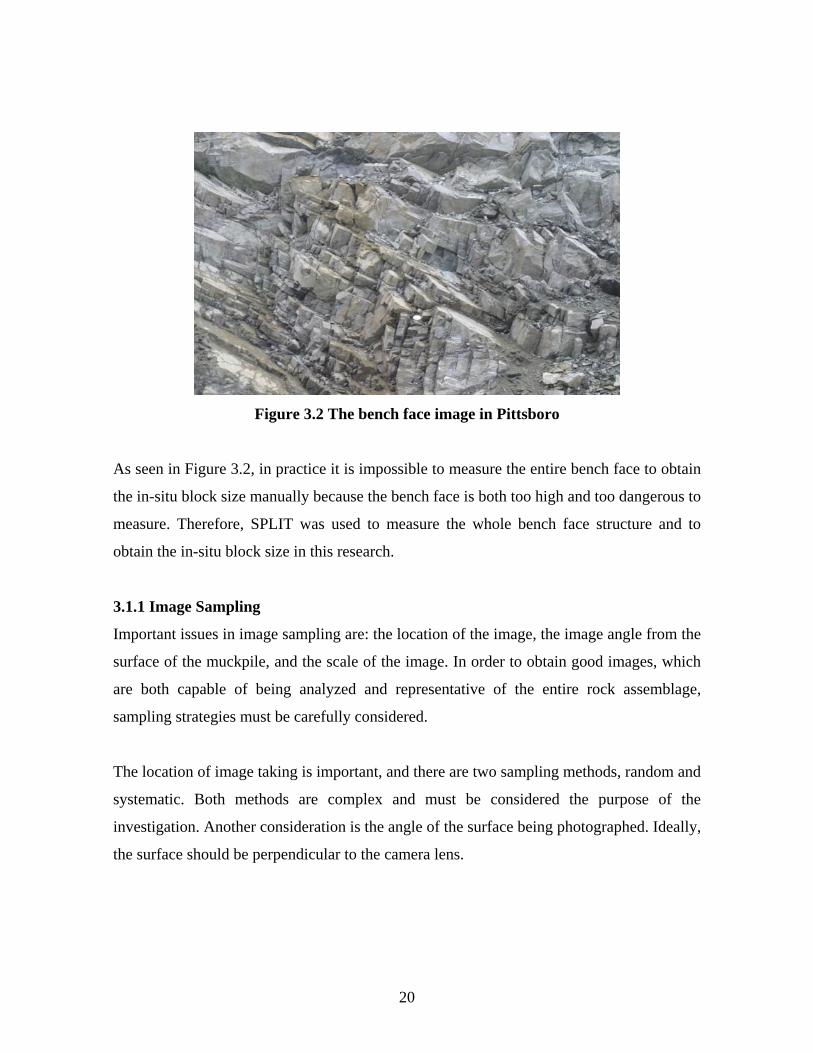
Figure 3.2 The bench face image in Pittsboro
As seen in Figure 3.2, in practice it is impossible to measure the entire bench face to obtain
the in-situ block size manually because the bench face is both too high and too dangerous to
measure. Therefore, SPLIT was used to measure the whole bench face structure and to
obtain the in-situ block size in this research.
3.1.1 Image Sampling
Important issues in image sampling are: the location of the image, the image angle from the
surface of the muckpile, and the scale of the image. In order to obtain good images, which
are both capable of being analyzed and representative of the entire rock assemblage,
sampling strategies must be carefully considered.
The location of image taking is important, and there are two sampling methods, random and
systematic. Both methods are complex and must be considered the purpose of the
investigation. Another consideration is the angle of the surface being photographed. Ideally,
the surface should be perpendicular to the camera lens.
20

Consistent sampling from image to image is the main strategy in this research and one of
the most important factors in the sampling strategy. Analyzed data show large variations
from image to image, but as a whole, the data demonstrate consistency. In a muckpile after
blasting, merely remaining consistent in sampling may not be sufficient to show the real
size distribution. This strategy saves time in sampling and is convenient for the blasting
engineer to make a site-specific model for quarry blasting.
The Image Sampling on a Bench Face
To consider the whole bench face, the in-situ block size on a bench face will be obtained by
using SPLIT program.
A digital camera was used to get the image of the bench face, which will be used in SPLIT.
The maximum size image that can be processed using SPLIT is 1680*1400 pixels, so the
maximum size image needs to be considered during sampling images because image
editing may be required in SPLIT, and a larger image may not be opened in SPLIT without
such editing.
Figure 3.3 The bench face image from Bosung quarry
21

Image samples were obtained during charging explosives after drilling for blasting.
Approximately five to seven (5-7) pictures were taken at each blasting, and three to five (3-
5) appropriate pictures for analyzing in SPLIT were chosen. Figure 3.3 is an example of
image sample. An article of known dimensions, a scale material, must be in the picture in
order to provide scale. A white plate was used as a scale material on the bench face. The
same scale material must be used from image to image for analyzing all pictures in SPLIT
regarding each blasting. Also, the number of scale materials should be the same from image
to image for analysis. Typically, only one scale material was used for the bench face image
analysis in this research.
The Image Sampling From a Muckpile After Blasting
Fragmentation assessment can be achieved by analyzing scaled photographs taken of the
muckpile. The digital camera should be held such that the long axis of the photograph is
vertical. The image should be taken with the camera lens perpendicular to the muckpile
surface (JKMRC, 1996).
Figure 3.4 The muckpile image from Bosung quarry
To provide scale in the photograph, a tennis ball was used. If the slope of a pile needs to be
shown, then two scale materials can be used as shown in Figure 3.4. These materials should
22

neither be placed randomly on the muckpile nor in a horizontal line across the muckpile. In
addition, the same number of scale materials should be used from sample to sample in the
same blasting site to analyze together in SPLIT.
As previously mentioned, the maximum image size is 1680*1400 pixels. If the size is too
large to be analyzed in SPLIT, then image editing is required.
A more representative sample may be obtained by photographing the material being loaded
into a truck or as a truckload is being dumped because the outside surface of a muckpile
before digging cannot represent the material within the pile. That means obtaining images
of the entire exposed surface of the pile to avoid biased results, however it takes longer to
acquire these images.
The main focus of sampling of muckpile images in this research is consistency rather than
representation. Therefore, the image samples after blasting were obtained directly from the
muckpile and five to seven images of the muckpile were captured and analyzed at each
blasting. To show as much of the muckpile as possible, each image sample was obtained at
the different part of a muckpile and overlapping images were avoided.
Safety is tantamount during sampling images from a muckpile. Scale material was thrown
to the dangerous site and the zoom function of a digital camera was used for sampling
purposes. It is especially dangerous near the bench face after blasting.
3.1.2 Image Analysis Using SPLIT
SPLIT, image analysis program, will be used for analyzing a bench face and a muckpile.
The block structure of bench in a quarry before blasting may be obtained by analyzing the
bench face, and the result of blasting will be estimated by using SPLIT on the muckpile.
23

Imgae analysis on a bench face
Consistency is the primary focus in the initial trial of the image analysis program used on
the bench face to obtain information regarding the in-situ block size.
Following is the important and specific setting at the step of Editing and Compute Size in
SPLIT for analyzing the bench face.
1. Only the scale material should be edited.
2. Zero percent (0%) of percent fines adjustment.
3. Rosin-Rammler was used for fines distribution.
Bench face images were not edited much in this study. Only the scale material and the other
parts of image except the bench face were edited. Therefore, the part of the bench face
image was not edited except for the actual scale material. If the bench face image is edited,
then the editing image is not sufficient because the crack on the bench face is often very
difficult to see. Although non-edited images analysis cannot reflect the real size distribution
of the block on the bench faces and contains errors, non-edited images revealed more
consistent analysis result than edited ones.
On the bench face, the fines are not considered because the bench face image analysis is for
obtaining information regarding the in-situ block size. Therefore the setting for fines
adjustment is zero percent (0%).
For the prediction of fines in SPLIT, there are three options - Schuhmann, Rosin-Rammler,
and best-fit. Any prediction model may be used, but the same model should be used from
image to image. The Rosin-Rammler model was chosen for this research.
At the step of Graphs and Outputs, this setting depends on the user. The setting of graphing
is “Cumulative”, and size axis and percent axis is “Linear” in this research. Figure 3.5
shows the bench face image analysis in SPLIT.
24

Figure 3.5 The analyzed bench face image of Bosung quarry in SPLIT
Image Analysis on a Muckpile
At the step of Editing and Compute Size in SPLIT, the important settings are as follows.
1. Fifty (50%) of percent fines adjustment (Medium).
2. Rosin-Rammler was used for fines distribution.
25

Usually one or two scale materials were used on the muckpile. If the angle of muckpile
surface needs to be considered then two scale materials were used. Of course, the number
of scale materials depends on the sampling situation.
Muckpile image analysis has the following limitations regarding fines estimation, so the
percent fines adjustment was set to “Medium.” The percent fines adjustment percentage
may be changed to twenty (20%), forty (40%), or sixty percent (60%), but the percentage
should be consistent from image to image. In this research, fifty percent (50%) was chosen
as the percent fines adjustment because this is the usual setting for muckpile image analysis
in SPLIT. Figure 3.6 shows the muckpile image and analyzed image in SPLIT.
Figure 3.6 The muckpile image and analyzed image in SPLIT
In addition, Rosin-Rammler model was used for prediction of fines. Users may choose the
prediction model. The situation is the same with the bench face image analysis.
Consistency of the model choice should be kept from image to image.
The setting of graphing is “Cumulative”, and size axis and percent axis is “Linear” at the
step of Graphs and Outputs in this research. This setting also depends on the user(s).
26

The Size Distribution Curves from a Bench face and a Muckpile
As the result of image analysis, two kinds of cumulative size distribution curve were
obtained from a bench face and a muckpile at each location.
Figure 3.7 The size distribution curves from the bench face (left) and muckpile (right)
Figure 3.7 shows size distribution curves. The left chart represents the result of the bench
face image analysis, and the right chart is the result of the muckpile image analysis.
From these size distribution curves, the data in Table 3.1 were obtained. These data are
analyzed, and will be used for making an empirical equation model. The unit in the table is
represented in millimeters. Prefix “F” and “P” before the % passing sizes represent bench
face and muckpile respectively.
27

Table 3.1 The data from the size distribution curve of the bench face and muckpile
F20 F50 F80 P20 P50 P80 Bosung1 165 410 810 46 255 493 Bosung2 245 586 937 23 214 428 Bosung3 196 420 821 91 226 431 Bosung4 158 285 467 72 209 335 Bosung5 178 330 551 93 252 499 Pittsboro 158 281 483 40 100 187 Boxley 514 929 1512 69 161 304 Sanyang1 102 192 334 55 179 350 Sanyang2 102 196 382 88 192 290 Sanyang3 114 211 360 24 89 199 Sanyang4 50 91 149 21 82 163 Sanyang5 81 164 309 31 144 265
F20, F50, and F80 in Table 3.1 are from the size distribution curve of a bench face. F20
means the twenty percent (20%) passing size in the size distribution curve of a bench face,
and F50 and F80 are the same as F20.
P20, P50, and P80 are similar with F20, F50, and F80. These are twenty (20%), fifty (50%),
and eighty percent (80%) passing size in the size distribution curve of the muckpile.
F50 and the Mean In-situ Block Size
The reason for the bench face analysis using SPLIT is to obtain information about the block
size. In Pitttsboro blasting, the mean in-situ block size was measured manually, and the size
is 0.2 meters. In Table 3.2, the scale of F50 (or F20) and the mean in-situ block size is
similar. Although more research will be needed, it shows the possibility that F50 may be
used as a new index of mean in-situ block size. In addition, reasonable results of data
analysis were shown with these data in Chapter 4.
Table 3.2 The data from the bench face, and the manually measured block size in Pittsboro
Location F20 F50 F80 Mean in-situ block Pittsboro 158 281 483 200
28
3.2 Calculation of KIC
Standardized experimental testing has not been developed to determine the fracture
toughness of rock. The critical value of stress intensity factor, KIC, may be determined
experimentally in different ways. Most methods involve intense sample preparation and
are then loaded under very specific conditions.
Donovan proposed a relatively easier test (Donovan and Karfakis, 2004). This test uses an
edge notched disk (END) sample loaded on a wedge of set geometry. The sample is then
loaded uniaxially until failure.
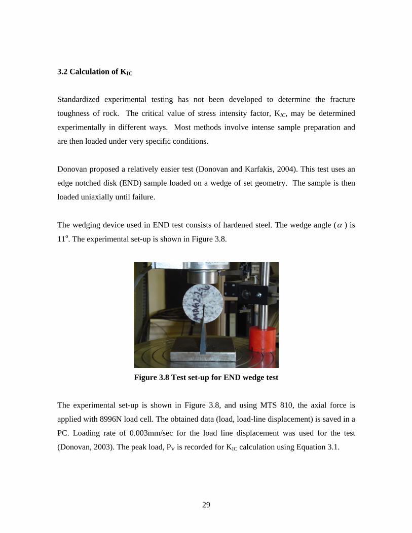
The wedging device used in END test consists of hardened steel. The wedge angle (α ) is
11o. The experimental set-up is shown in Figure 3.8.
Figure 3.8 Test set-up for END wedge test
The experimental set-up is shown in Figure 3.8, and using MTS 810, the axial force is
applied with 8996N load cell. The obtained data (load, load-line displacement) is saved in a
PC. Loading rate of 0.003mm/sec for the load line displacement was used for the test
(Donovan, 2003). The peak load, PV is recorded for KIC calculation using Equation 3.1.
29

( ) taDaDa
aD
IC1.
)(966528.01
355715.02
cot1
2tan1
*
2tan22
2 2/12/3 ⎟⎟⎠
⎞−
+⎜⎜⎝
⎛
−⋅⎟⎟⎟⎟
⎠
⎞
⎜⎜⎜⎜
⎝
⎛
⎟⎠⎞
⎜⎝⎛+
⎟⎠⎞
⎜⎝⎛−
⎟⎠⎞
⎜⎝⎛
Ρ⋅⋅=Κ
αµ
αµ
αν (3.1)
Where: Pv = the applied peak load
α = the wedge angle
µ = friction coefficient
a = the notch length
D = specimen diameter
The peak load and friction coefficient are used in Equation 3.1 to determine the fracture
toughness.
The sample properties and geometric values used in this study were taken from experiments.
The angle of wedge is eleven degrees (11o). A tilt test was used to determine friction
coefficient ( µ ) on hardened steel. The sliding angle is φ and tanφ is equal to µ . The
friction coefficients for the four quarry rocks are given in Table 3.3.
Table 3.3 Values of φ andµ of four quarries rock
Friction Coefficient (µ )
Rock Type φ (degree) µ
Pittsboro 24.0± 1.11 0.445 Boxley 24.8± 3.03 0.462 Bosung 30.1± 2.14 0.580 Sanyang 27.2± 1.67 0.514
Table 3.4 shows mode I fracture toughness, tensile strength, and specific gravity values for
the rocks in the four quarries.
30

Table 3.4 Fracture toughness, KIC, Tensile strength, tσ , and Specific Gravity
Location KIC(MPa*m^0.5) tσ (MPa) Specific Gravity (t/m3)
Pittsboro 1.539± 0.100 16.94± 1.92 2.69 0.06 ±
Boxley 1.724± 0.193 17.45± 2.57 2.73 0.01 ±
Bosung 1.889± 0.398 22.48± 4.70 2.58 0.05 ±
Sanyang 1.230± 0.216 14.72± 1.23 2.49 0.07 ±
3.3 Blasting specific explosives energy
Specific energy for fragmentation is the explosive or mechanical energy required to
fragment a unit of volume or mass of rock (Rustan, 1998). The Specific Explosives Energy
(ESE) in this research represents the blasting energy required to fragment a unit of mass of
rock. Therefore the unit is “wh/tonne”. This value is affected by a blasting pattern
(explosives amount, bench height, burden, spacing, hole diameter, rock specific gravity,
and the type of explosives), consequently ESE can be assumed to represent the blasting
pattern and can be determined using Equation 3.2.
S.G.(ton)SpacingBurdenHeighthole(wh)per Energy Explosives×××
=SEE (3.2)
Explosives energy per hole is affected by the diameter of the hole, bench height, and type
of explosives. The explosives amount per hole was estimated as the average explosives
amount per hole in this research.
Powder factor is the quantity of explosives used per unit of rock blasted (Kg/ton or Kg/m3).
An accurate prediction of powder factor in blasting is needed for optimal blasting to reduce
operation costs (drilling, blasting, loading, haulage and crushing). Powder factor is one of
the most important tools used to design the blasts (Jimeno and Carcedo, 1995). Since ESE is
conceptually same with powder factor, ESE prediction will be evaluated for optimal blasting
31

pattern by using an empirical equation model in this study. Blasting pattern for Pittsboro
and Specific Explosives Energy (ESE) are tabulated in Table 3.5.
Table 3.5 Blasting pattern and ESE in Pittsboro blasting
Blasting pattern and ESE Pittsboro Unit
Bench Height 19.8 m Burden 4.57 m Spacing 4.57 m
Rock Specific Gravity 2.69 t/m^3 Hole diameter 165 mm
Explosives Hydromite4400
Explosives amount per hole 429 kg Explosives energy per gram 863 Kcal/Kg
Explosives energy per hole 431 Kwh Specific Explosives Energy (Ese) 387 wh/tonne
3.4 The Main Issues in SPLIT for the Research (Norton, B., 2005)
There are various issues in the use of SPLIT. The concepts, P50, fines, the fines percent
adjustment in a muckpile, and the size of images, were considered as described below.
An Average Size and P50 in SPLIT
The P50 is not necessarily the average size, but is fifty-percent (50%) passing size by
weight. That means the P50 is not the mean size in terms of dimension. It is the mean size
by weight. Half of the volume or weight is less than this size particle. It is assumed the
particles have all the same density, so the terms of volume and weight can be used
interchangeably.
Larger or Smaller Image
When the muckpile was evaluated, the smaller image would definitely be more efficient
because it is smaller and closer to the size of the material. A larger image would be less
32

efficient as it takes longer to edit. However, a larger image provides more particles for the
sample, so there is a tradeoff. When the bench face was evaluated, the small and large
images showed similar results of image analysis. Once again, the main focus is keeping
scale consistent from image to image.
Fines
Smaller particles are hidden under the larger particles and are not visible. The resolution of
the image is such that the software can only measure down to a certain point. Therefore the
empirical model, either Rosin-Rammler or Schumann, below the point of the size
distribution curve, predicts the size distribution. The curve color is a little changed at that
point from that at which the size distribution is predicted by the empirical model in SPLIT.
The Selection of the Fines Percent Adjustment in a Muckpile
The key is not to change the setting from sample to sample. The default setting is fifty
percent (50%) and this is what many people use ninety-nine percent (99%) of the time
when analyzing muckpile images. This is because we do not have sieve results and we want
to be able to compare curves knowing the same setting was used to generate them. The
evaluation of images from a blast muckpile is particularly difficult due to its size, depth and
internal variations.
To obtain information of the in-situ block size on the bench face, the default setting is zero
percent (0%) because fines analysis on the bench face are not needed for this study, and the
key is keeping the setting consistent from image to image.
33

Chapter 4 – Data Analysis
Donovan has developed a model to predict the specific comminution energy, EC, in jaw
crushers using the HECT system. Following is one of the Donovan’s models (Donovan and
Karfakis, 2004).
([ ] ICc KRRE 511.0511.0 +−= )5.11 <≤ RR
[ ] ICc KRRE 425.0215.0= ( ) 5.1≥RR [ ]tkwh /
The unit of Ec is kilowatt-hours per metric ton and reduction ratio is defined as the particle
size divided by the closed side set of a jaw crusher.
Conceptually ESE and Donovan’s EC are similar with each other. Thus, the prediction
model, , is assumed, and data analysis is performed using this proposed
equation.
cSE aE IC
b K RR =
For the assessment of rock blasting, four factors should be considered (Cunningham, 1987)
and (JKMRC, 1996).
(1) Rock density
(2) Mechanical strength (UCS)
(3) Elastic properties (Young’s modulus)
(4) Structure (In-situ block size)
Mechanical strength is related with the Uniaxial Compressive Strength (UCS), and UCS
has been used as mechanical strength in usual blasting model. However, the Uniaxial
Tensile Strength (UTS), measured by the Brazilian test, has a better correlation with rock
fracturing. Especially, fracture toughness has a strong relationship with the tensile strength
of rock, and further, a good correlation with energy consumption for rock fragmentation in
a crusher (Donovan, 2003). Thus, the rock properties, mechanical strength and elastic
34

modulus, will be replaced by the KIC, fracture toughness, in the empirical blasting model in
this study.
Assumed energy prediction equation form contains following meanings:
- ESE is affected by a blasting pattern (Bench height, burden, spacing, hole diameter, and
explosives amount) and rock density, so ESE will represent a blasting pattern in the model.
- RR reflects both whole benches face structure (In-situ block size, F) and the desired
fragment size (P) after blasting.
- KIC represents rock properties for prediction of explosives energy consumption.
Therefore, assumed equation form contains the necessary factors for assessment of rock
fragmentation and includes target fragment size, P80.
4.1 The Equation Model
Table 4.1 summarizes the blasting and rock property data from twelve blasts in the four
quarries. The bench face and the muckpile information are represented by “F” and “P”
respectively. The data in Table 4.1 is analyzed using the proposed equation,
. cSE aE IC
b K RR =
Table 4.1 The obtained data of blasting
ESE KIC F20 F50 F80 P20 P50 P80 RR20 RR50 RR80
Bosung1 103 1.539 165 410 810 46 255 493 3.6 1.6 1.6 Bosung2 103 1.539 245 586 937 23 214 428 10.8 2.7 2.2 Bosung3 107 1.539 196 420 821 91 226 431 2.2 1.9 1.9 Bosung4 107 1.539 158 285 467 72 209 335 2.2 1.4 1.4 Bosung5 110 1.539 178 330 551 93 252 499 1.9 1.3 1.1 Pittsboro 387 1.724 158 281 483 40 100 187 4.0 2.8 2.6
Boxley 268 1.230 514 929 1512 69 161 304 7.4 5.8 5.0 Sanyang1 268 1.889 102 192 334 55 179 350 1.8 1.1 1.0 Sanyang2 292 1.889 102 196 382 88 192 290 1.2 1.0 1.3 Sanyang3 336 1.889 114 211 360 24 89 199 4.8 2.4 1.8 Sanyang4 222 1.889 50 91 149 21 82 163 2.4 1.1 0.9 Sanyang5 210 1.889 81 164 309 31 144 265 2.6 1.1 1.2
35

4.1.1 Specific Explosives Energy, KIC and RR80
Following data in the table shows that ESE is correlated with RR80 and KIC value.
Table 4.2 ESE with given KIC and RR80
Location ESE(Wh/tonne) KIC(Mpa*m1/2) RR80
Bosung1 103 1.539 1.6 Bosung2 103 1.539 2.2 Bosung3 107 1.539 1.9 Bosung4 107 1.539 1.4 Bosung5 110 1.539 1.1 Pittsboro 387 1.724 2.6 Boxley 268 1.230 5.0 Sanyang2 292 1.889 1.3 Sanyang3 336 1.889 1.8 Sanyang5 210 1.889 1.2
In Bosung and Sanyang quarries, each blasting location was close to the other, so the rock
property, KIC value was assumed to be the same within the same quarry blasting in this
study. Therefore, although END test was just conducted for KIC value from Bosung1 and
Sanyang1 blasting, the other blasted rock in Sanyang and Bosung were assumed as the
same with Bosung1 and Sanyang1 at each.
There is the reduction ratio for 80% passing for blast 1 and 4 at the Sanyang quarry, but
consequently the data was omitted from the analysis. The reason is that although explosives
energy was given, breakage was not realized and the entire blasting energy was consumed
to release the block on the bench.
In Table 4.2, regression analysis in EXCEL and SAS was fit to the proposed model, and
both programs gave the same result.
ESE= 11.7 RR801.202 KIC
4.14 (4.1)
Where:
ESE is specific explosives energy (wh/ton).
36

RR80 is the reduction ratio based on 80% passing.
KIC is the Mode I fracture toughness of rock.
Figure 4.1 shows the accuracy between predicted specific explosives energy using Equation
4.1 and actual specific explosives energy with the given RR80 and KIC
050
100150200250300350400450
0 1 2 3 4 5 6 7 8 9 10 11
Blasting
Ese (wh/ton) Actual Ese
Predicted Ese
Figure 4.1 The accuracy between predicted ESE and ESE with given RR80 and KIC
Since there are just ten (10) blasting data, statistically there is not enough data to make the
equation model. However, predicted ESE is in agreement with ESE as seen in Figure 4.1. The
plot of Equation 4.1 with respect to KIC is shown in Figure 4.2.
37

0
100
200
300
400
500
600
700
800
1 1.2 1.4 1.6 1.8 2 2.2 2.4 2.6 2.8 3
RR80
Energy (wh/ton)
Kic=1.0
Kic=1.2
Kic=1.3
Kic=1.4
Kic=1.5
Kic=1.6
Kic=1.7
Kic=1.8
Kic=1.9
Kic=2.0
Figure 4.2 Predicted ESE for RR80 and given KIC
Figure 4.2 means that:
- ESE and RR80 are in proportion. That means larger RR80 needs more specific explosives
energy to fragment.
- ESE and KIC are also in proportion, thus the rock having larger KIC is required more
specific explosives energy for breakage.
Larger RR means more breakage, and the rock having larger KIC is harder to fragment.
Therefore, these relationships based on Equation 4.1 are reasonable.
RR50 and RR80
It is interesting that RR50 and RR80 have similar values in Table 4.2. Therefore, the
relationship among ESE, KIC and RR50 is similar with RR80’s. Figure 4.3 shows the
similarity between RR50 and RR80.
38

RR50 and RR80
0.0
0.5
1.0
1.5
2.0
2.5
3.0
0.0 0.5 1.0 1.5 2.0 2.5 3.0
RR50
RR80
Figure 4.3 RR50 and RR80
The equation is also similar with Equation 4.1, which is about RR80.
ESE = 15.0 RR500.86 KIC
4.02 (4.2)
Thus, the relationship between ESE and RR50 is in proportion, and the relationship between
ESE and KIC is also in proportion. That means more explosives energy is required for more
breakage (larger RR50) and harder rock (larger KIC).
4.1.2 Specific Explosives Energy, KIC and RR20
Table 4.3 shows the data for analyzing the relationship between RR20 and ESE with given
rock fracture toughness, KIC.
39

Table 4.3 ESE with given KIC and RR20
Location ESE(Wh/tonne) KIC(Mpa*m1/2) RR20
Bosung1 103 1.539 3.6 Bosung2 103 1.539 10.8 Bosung3 107 1.539 2.2 Bosung4 107 1.539 2.2 Bosung5 110 1.539 1.9 Pittsboro 387 1.724 4.0 Boxley 268 1.230 7.4 Sanyang1 268 1.889 1.8 Sanyang2 292 1.889 1.2 Sanyang3 336 1.889 4.8 Sanyang4 222 1.889 2.4 Sanyang5 210 1.889 2.6
Using regression of EXCEL and SAS program, data analysis has been tried, and the
equation was obtained.
ESE=49.0 RR200.20 KIC
2.19 (4.3)
Where:
- RR20 is the reduction ratio based on 20% passing.
However, the relationship was not in good agreement as seen in Figure 4.4, and the points
of the accuracy graph were just scattered.
40

0
50
100
150
200
250
300
350
400
450
0 50 100 150 200 250 300
Pred.Ese (Wh/ton)
E (Wh/ton)
Figure 4.4 Accuracy between predicted ESE and ESE with given RR20 and KIC
The reason is that:
- SPLIT, image analysis program has the limitation of estimating fines in the muckpile.
Usually P20 is near fines size in the distribution curve of muckpile image analysis.
- Muckpile image sampling has just done from the surface of a muckpile. However, as seen
in Figure 4.5 upper part rock of the muckpile is just liberated from the bench, and the lower
part rock is broken (JKMRC, 1996).
Figure 4.5 Liberated versus broken rock in the Pittsboro blast (JKMRC, 1996)
41

The lower part of the muckpile should be investigated to determine fines or small sizes of
rock distribution in the muckpile. Thus, a sieving test is needed to analyze RR20 or P20 in
the muckpile, or image sampling may be done from a hauling truck, although it will take
considerable time.
- Blasting data are too short to investigate the real relationship and to determine some
models.
The sampling method and analysis tool in these blastings is not good enough to obtain fines
in this research.
Although predicted ESE is not in agreement with given RR20 and KIC, the result is
reasonable because there is the limitation of SPLIT usage and image sampling method in
this research. The disagreement of relationships among RR20, KIC, and ESE is rather
reasonable.
4.1.3 P50 and P80
The two factors, P50 and P80 are in proportion as the change of uniformity index, N from
Rosin-Rammler model.
808.0ln5.0ln50
/1
PPN
⎟⎠⎞
⎜⎝⎛= (4.4)
Where:
P50: 50 % passing size from the size distribution curve in a muckpile after blasting
P80: 80% passing size from the size distribution curve in a muckpile after blasting
N: The Uniformity index from Kuznetsov (Kuznetsov, 1973)
The Equation 4.4 can be derived from the following Rosin-Rammler equation.
n
Cxx
eR )(−=
42

Where:
R is the fraction of material retained on screen
X is the screen size
XC is characteristic size, constant
N is uniformity index, constant
Thus, P50 is n
CxP
e )50(5.0 −= , and P80 is n
CxP
e )80(8.0 −= in Rosin-Rammler model.
If natural logarithm is used in the both above equations, then both equations will be as
following:
ln 0.5 = - (P50/XC)N and ln 0.8 = - (P80/XC)N
Thus, NC
NC
XPXP
)/80()/50(
8.0ln5.0ln
−−
=
Then, 808.0ln5.0ln50
/1
PPN
⎟⎠⎞
⎜⎝⎛=
Cunningham suggested Equation 4.5 to determine uniformity index as following
(Cunningham, 1983 and 1987).
1.0)or 1.1(1.012/1142.2
1.05.0
×⎟⎟⎠
⎞⎜⎜⎝
⎛+
+−
⎟⎠⎞
⎜⎝⎛ −⎟
⎠⎞
⎜⎝⎛ +⎟⎠⎞
⎜⎝⎛ −=
HL
LLLL
BWBS
DBN
CB
CB (4.5)
Where:
D is the hole diameter in mm,
B is the burden in m,
W is the standard deviation of drilling accuracy in m,
S is the spacing in m,
43

LB in the bottom charge length in m,
LC is the column charge length in m,
L is the total charge length in m,
H is the Bench height in m.
If a staggered blasting pattern was employed, then the uniformity index will be increased
by ten percent (10%).
In the quarry blasting with similar bench height and hole diameter, the change of total
charge length, L, and the standard deviation of drilling accuracy, W, is limited.
Therefore, the range of (log0.5/log0.8)1/N is just (+/-) 0.1 as (+/-) 2 meters change burden
and spacing with the same bench height and hole diameter in the blasting pattern from
Equation 4.4 and 4.5.
Derived Equation 4.4 shows that the relationship between P50 and P80 will be in
proportion in quarries blasting which have the similar bench height and hole diameter.
Bosung (1,2,3,4) and Sanyang blasting (4,5) have similar bench height, 11m, and hole
diameter, 76mm. Table 4.4 is the blasting data of P50 and P80 in Bosung and Sanyang
quarry.
Table 4.4 P50 and P80 in Bosung and Sanyang
Location P50(mm) P80(mm)Bosung 1 255 493 Bosung 2 214 428 Bosung 3 226 431 Bosung 4 209 335 Sanyang 4 82 163 Sanyang 5 144 265
The data of “P50 and P80” from Table 4.4 was analyzed using EXCEL regression, and the
following relationship was obtained.
P50=0.5P80 (4.6)
44

Where:
P50: 50 % passing size from the size distribution curve in a muckpile after blasting
P80: 80% passing size from the size distribution curve in a muckpile after blasting
Figure 4.6 shows the accuracy of predicted P50 using Equation 4.6.
0
50
100
150
200
250
300
0 50 100 150 200 250 300
Pred. P50(mm)
P50(mm)
Figure 4.6 The accuracy between predicted P50 and P50
If there is the same bench height and hole diameter at the blasting sites, then P50 may be
predicted with P80 from blasting to blasting. Although data is insufficient to determine the
actual relationship between P50 and P80, there should be a proportional relationship
between P50 and P80 in blasting with the same bench height and hole diameter because it is
both theoretically and practically reasonable.
Again, to make a site-specific empirical blasting model, this relationship between P50 and
P80 is useful because the bench height and hole diameter is usually similar or the same
within each quarry.
45

Chapter 5 Discussion of Results
5.1 Improvements Revealed by the Research
1. SPLIT was used successfully to examine the bench face.
Using SPLIT on the bench face was effective and produced reasonably consistent results.
F50 in SPLIT on the bench face can be a new index as the mean in-situ block size. Actually,
the manually measured mean in-situ block size and F50 in SPLIT on the bench face share
the similar scale in the Pittsboro quarry.
2. The Kuz-Ram model was adapted as a practical means for predicting size distribution in
the muckpile.
In the Kuz-Ram model, the average size of rock in the muckpile and the size distribution
curve were predicted using given factors in the blasting site. However, in this research,
because the products (P80) were what we wanted, the desired P80 was taken for granted,
and P50 predicted by the empirical model; proper burden and spacing were predicted by
using the empirical model with the given blasting factors. In addition, the size distribution
curve in the muckpile was predicted with P50 and proper burden & spacing based on the
given factors. P80, the eighty percent (80%) passing size, was assumed to be the optimum
size desired by most model users and the representative size of the muckpile.
3. An attempt was made to use Mode I fracture toughness as the rock property in the
blasting model instead of UCS (Uniaxial Compressive Strength) and E (Young’s modulus)
in Kuz-Ram.
Although tensile strength has a strong correlation with rock breakage, only UCS and E are
used in Kuz-Ram. In our study Mode I fracture toughness was used in the blasting model
because tensile strength has strong relationship with KIC.
46

Mode I is the most commonly encountered mode of crack deformation in rock blasting
applications. However, although the relationship between KIC and the size distribution of
blasting result could be determined, the data was insufficient to figure out the correlation.
Additional sieving tests seemed reasonable and justifiable. In addition we discovered that
KIC may especially correlate with fines and the small size of rock in the muckpile's whole
size distribution. However, further research is needed regarding these issues because the
data is insufficient to make a final determination and an image analysis program has the
disadvantage of underestimation of fines in the muckpile.
4. Although this model is not specific to any blasting area because of the shortage of
blasting data, it may be adapted by blasting engineers to particular mines for the purpose of
making a site-specific model.
The empirical model was derived step by step as follows:
• Collect blasting image data (the bench face and the muckpile image)
and rock sample after blasting.
• Conduct the END test with sampled rock.
• Analyze collected data using image analysis.
• Conduct regression using SAS or EXCEL with suggested equation form.
• Adjust the empirical equations for specific blasting sites.
• Use this adjusted empirical equation model in the simulation model based on
Visual Basic. NET program.
Thus, it would seem that an organized blasting design with the desired consistent result,
P80, may be possible.
47

5.2 The Bench Face Structure and the Blasting Design for Desired Consistent Results
Optimized blasting in mining is a complex issue because the entire detailed process must be
considered. Optimized blasting is different at each blasting site because there are different
crushers, drilling machines, hauling machines, and bench height considerations. However,
whether or not blasting is optimized, organized blasting for consistent results based on a
simple and flexible blasting model will greatly reduce energy waste.
If there is a given bench height and diameter of the drilling hole at the blasting site, then
burden and spacing are two of the most important factors in the blasting model because
these factors are easy to manipulate, whereas other factors are more difficult to control.
Therefore, application of the model has been focused on obtaining proper burden and
spacing to obtain the desired blasting result by using the site-specific blasting equation
model consistently.
To obtain consistent blasting results, one of the greatest obstacles in a given blasting site is
accurate determination of changes in the bench face structure. Although the rock properties,
bench height, and hole diameter are the same from blasting to blasting in a given blasting
site, the bench face structure is almost always changed during each blasting.
In this research, the change of bench face structure was measured easily and quickly using
the image-processing program. As with the change of the bench face structure (size ‘F’),
the burden and spacing in a blasting pattern were likewise adjusted for each blasting site.
5.3 P80 for the Optimal Blasting in a Quarry (Kojovic, 2006)
Practically, for a typical quarry, waste is below 0.005m, the desired final product size
ranging from 0.005 to 0.025m. That means everything above 0.025m has to be reduced.
This is typically done via blasting followed by multi-stage crushing. The amount of
48

blasting will clearly impact the amount of crushing required, so the trick is to find the
optimum level of blasting to maximize the yield of 0.005~0.025m product, at the lowest
overall cost (of drilling, blasting, and crushing, including the cost of energy, liners and
maintenance). Too much blasting can lead to too many fines, which may well reduce the
amount of crushing required at the expense of lowering the overall yield. Too little initial
crushing might require more crushing later in the process, which means more electrical
energy and more wear and tear on the equipment, with the result that costs go up once again.
Ideally, each quarry will maintain an optimum balance between the blasting and crushing
required to achieve the best possible outcome. Because rock conditions will dictate what
these balances should be, it is not enough to target just one size (P80). However, in
practice, targeting a P80 of 0.2m in the blast might be great in terms of the reduced
crushing requirements, but the blast would have to be too energetic, resulting in too much
waste, that is to say, anything less than 0.005m. We are therefore looking for the best
balance to achieve the optimum yield and lowest overall cost. To consider blasting as an
isolated process is to ignore the possible negative impact downstream.
P80 may be just a convenient yardstick on the level of coarseness in the blasting model, but
the predicted size distribution curve was obtained by using P80, resulting in proper burden
and spacing in the research model. Thus, a closed design for optimization in a quarry
process may be obtained by manipulating the blasting design (burden, spacing, and desired
P80) in the model. In the mine to mill optimization project (Virginia Tech and JKMRC
2004~2006), the optimized blasting came up with a P80 range of 0.2~0.3m. This range may
be used as the P80 size for optimized blasting in a usual quarry.
5.4 Generalized Blasting Model
A generalized blasting model is difficult to devise because rock properties and bench face
structure vary greatly, and obtaining blasting data is both expensive and time-consuming.
Actually, a generalized model may be unattainable because every blasting model must be
49

adjusted for the given blasting site. With this in mind, in constructing the present model just
twenty or thirty pieces of blasting data were used per given blasting site. This model may
be more powerful and efficient than any other blasting model within a given blasting site.
Using the method described in this thesis, will assist blasting engineers in achieving more
efficient blasting in their quarries and provide a much-needed reduction in the amounts of
energy used in the mining process.
5.5 Application for the Simulation Model
Using the obtained empirical equation models and adjusted Kuz-Ram model, the simulation
program can be made with Visual Basic.NET program.
Although the following simulation program is not truly sufficient for definitive conclusion,
this practical trial will be useful for making a site-specific blasting model simulation for
blasting engineers.
1. Given Factors in the model *Blasting pattern - H,D : Bench height(m)/ Hole diameter(mm) - Ex. : Explosives amount (Kg, per hole) - L : Charge length (m) - W : Drill accuracy Standard Deviation(m) *Rock properties - SG : Rock Specific Gravity (tonne/m3) - KIC : Fracture toughness (Mpa*m0.5) *The block structure on the bench face - F80 : The in-situ block size (m) *The goal of the blasting - P80 : Wanted P80 in the muckpile size distribution (m) 2. The empirical model from the data analysis using regression - ESE = 11.7 RR80
1.202 KIC4.14
- P50 = 0.5 P80 P50
50

3. The adjusted model from the empirical model
⎟⎠⎞
⎜⎝⎛
××⎟⎟⎠
⎞⎜⎜⎝
⎛××
=×HGS
ExKRR
SBIC ..
.)()(7.11
11.42.1
80
B*S
4. The uniformity index (with above burden and spacing)
1.0)or 1.1(1.012/1142.2
1.05.0
×⎟⎟⎠
⎞⎜⎜⎝
⎛+
+−
⎟⎠⎞
⎜⎝⎛ −⎟
⎠⎞
⎜⎝⎛ +⎟⎠⎞
⎜⎝⎛ −=
HL
LLLL
BWBS
DBN
CB
CB B*S
5. Characteristic size (with above P50)
NCPX /1)693.0(
50= P50
6. Percent passing(%)
))exp(1(100)1(100 N
CP X
XRP −−=−= Predicted Size Distribution
The previous flow chart shows the mechanism of the following simulation program in
Figure 5.1. Using this mechanism, the following simulation can be made.
The suggested application is to obtain the proper burden and spacing with given hole
diameter, bench height, explosives amount, and the kind of explosives as the change of the
rock and the bench structure.
Above used equation in second blank of the flow chart, ESE = 11.7 RR801.202 KIC
4.14 was
obtained from 10 blasting data analysis, but another equation, (P50) = 0.5 (P80) is just from
6 blasting data analysis, both models were derived from the different number of blasting
data. However, the above application is just for showing how to make the model practical
using an empirical equation model. In addition, especially, the given factors (explosives
51

amount, charge length, and the kind of explosives) were based on the previously
experienced blasting patterns in a given blasting site.
Figure 5.1 Simulation using Visual Basic. Net Program
The above simulation model contains the whole necessary factors for assessment of rock
fragmentation (rock density, mechanical strength, elastic properties, and structure) and
includes target fragment size, P80.
Using the above simulation program, proper burden and spacing may be predicted for
desired P80 in the muckpile. In addition, predicted size distribution curve will be obtained
using adjusted Kuz-Ram model.
Thus, proper burden and spacing may be changed and adjusted for desired size distribution
in the muckpile.
52
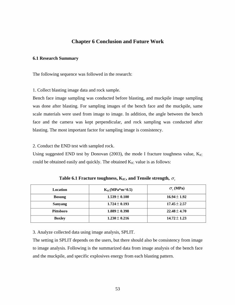
Chapter 6 Conclusion and Future Work
6.1 Research Summary
The following sequence was followed in the research:
1. Collect blasting image data and rock sample.
Bench face image sampling was conducted before blasting, and muckpile image sampling
was done after blasting. For sampling images of the bench face and the muckpile, same
scale materials were used from image to image. In addition, the angle between the bench
face and the camera was kept perpendicular, and rock sampling was conducted after
blasting. The most important factor for sampling image is consistency.
2. Conduct the END test with sampled rock.
Using suggested END test by Donovan (2003), the mode I fracture toughness value, KIC
could be obtained easily and quickly. The obtained KIC value is as follows:
Table 6.1 Fracture toughness, KIC, and Tensile strength, tσ
Location KIC(MPa*m^0.5) tσ (MPa)
Bosung 1.539± 0.100 16.94 1.92 ±
Sanyang 1.724± 0.193 17.45 2.57 ±
Pittsboro 1.889± 0.398 22.48 4.70 ±
Boxley 1.230± 0.216 14.72 1.23 ±
3. Analyze collected data using image analysis, SPLIT.
The setting in SPLIT depends on the users, but there should also be consistency from image
to image analysis. Following is the summarized data from image analysis of the bench face
and the muckpile, and specific explosives energy from each blasting pattern.
53

Table 6.2 Blasting data from image analysis, END test, and the blasting pattern
ESE KIC F20 F50 F80 P20 P50 P80 RR20 RR50 RR80
Bosung1 103 1.539 165 410 810 46 255 493 3.6 1.6 1.6 Bosung2 103 1.539 245 586 937 23 214 428 10.8 2.7 2.2 Bosung3 107 1.539 196 420 821 91 226 431 2.2 1.9 1.9 Bosung4 107 1.539 158 285 467 72 209 335 2.2 1.4 1.4 Bosung5 110 1.539 178 330 551 93 252 499 1.9 1.3 1.1 Pittsboro 387 1.724 158 281 483 40 100 187 4.0 2.8 2.6
Boxley 268 1.230 514 929 1512 69 161 304 7.4 5.8 5.0 Sanyang1 268 1.889 102 192 334 55 179 350 1.8 1.1 1.0 Sanyang2 292 1.889 102 196 382 88 192 290 1.2 1.0 1.3 Sanyang3 336 1.889 114 211 360 24 89 199 4.8 2.4 1.8 Sanyang4 222 1.889 50 91 149 21 82 163 2.4 1.1 0.9 Sanyang5 210 1.889 81 164 309 31 144 265 2.6 1.1 1.2
4. Conduct regression using SAS or EXCEL with suggested equation form.
Using the assumed equation form to predict the specific explosives energy, regression was
examined using SAS and EXCEL and the same constants were obtained. Actually, there
were about 80 kinds of analysis trials, from which the following results were selected.
ESE = 11.7 RR801.202 KIC
4.14
ESE = 15.0 RR500.86 KIC
4.02
ESE = 49.0 RR200.20 KIC
2.19
Where:
ESE is specific explosives energy (wh/ton).
RR80 is the reduction ratio based on 80% passing.
F80 is 80% passing size from the bench face image analysis (mm).
P80 is 80% passing size from the muckpile image analysis (mm).
RR20 and RR50 are same as RR80.
F50 is 50% passing size from the bench face image analysis (mm).
KIC is the Mode I fracture toughness of rock (MPa*m1/2).
In addition, the relationship between P50 and P80 was derived from the Rosin-Rammler
model.
54

808.0ln5.0ln50
/1
PPN
⎟⎠⎞
⎜⎝⎛=
P50 = 0.5 (P80)
5. Use the empirically obtained equation models for making the site-specific blasting model.
In this research, the following two equation models were selected for this application.
ESE = 11.7 RR801.202 KIC
4.14
P50 = 0.5 (P80)
6. Make the simulation model based on Visual Basic.NET program.
For convenience of usage, the language program VB.NET was used and a simulation
program was created. With this simulation program, proper burden and spacing can be
predicted for the target fragment size, P80, and P50 is predicted automatically. In addition,
the size distribution is predicted for the given blasting factors. Using this predicted size
distribution in reverse allowed us to adjust burden and spacing and target size, P80, in the
muckpile to achieve the desired size distribution.
For an example of the program usage,
1. At the given site, a blasting engineer wants to have the specific target fragment size, P80,
in the muckpile which is based on previous blasting data analysis at this site.
2. The rock properties and the bench face structure are totally different at each blast, but the
bench height and hole diameter are usually the same at each blast within the given blasting
site. Therefore, the blasting engineer uses the same blasting pattern (hole diameter, boring
depth, explosives, and explosives amount) except burden and spacing at each blast.
3. The blasting engineer conducts END wedge splitting test to obtain KIC, and uses the
image analysis program on the bench face to obtain the in-situ block size information.
55

4. The equation models, obtained by the current research, are used to get the proper burden
and spacing for the target fragment size, P80, in the muckpile.
Using this program, it is important to note that the blasting parameters, with the exception
of burden and spacing, are set equal to those used previously at the site.
6.2 Conclusion
Two main ideas were combined in this study. First, the whole bench face structure
information may be obtained by using an image-processing program, and this information
can be used for the blasting model. Secondly, mode I fracture toughness, KIC, can be used
to represent the rock properties in the blasting energy prediction model.
In the research, these two ideas were investigated to determine whether these ideas are
practical. The largest drawback in this investigation was the small amount of blasting data.
To create a new empirical blasting model and to test the new ideas in this blasting model,
twelve pieces of blasting data from four quarries was not enough.
However, if we consider that obtaining blasting data requires much time and expense, the
data, although insufficient, may be used to determine certain possibilities.
Basically, if we consider the concept of RR, ESE, and KIC, in the blasting energy prediction
model, then the following relationships are reasonable and may be hypothesized:
- ESE and RR will be in proportion.
- ESE and KIC will also be in proportion.
- The in-situ block size, F and ESE will be in inverse proportion because of leaking energy
of the explosives.
56

There follow the main empirical equation models obtained from the blasting data analyzed
in this research:
ESE = 11.7 (RR80)1.202 KIC
4.14
P50 = 0.5 (P80)
The above equations were not generalized because of the lack of data. However, the
research results are consistently reasonable, especially the findings (1) that ESE and KIC
with given RR80 are in proportion and (2) that ESE and RR are in proportion with given KIC,
and (3) that P50 and P80 are in proportion within a given bench height and hole diameter.
Using SPLIT on the bench face to get in-situ block sizes (F) was the first challenge. At each
image, the result of the SPLIT analysis reveals significant variability, but it also
demonstrated consistency on the whole, and it is a reasonable challenge because the
equation model is reasonable based on data analysis. Furthermore, in a blasting model, the
actual properties of the rock may be replaced by the rock fracture toughness, KIC to predict
the energy consumed in blasting.
Thus, although blasting data is insufficient to determine a model and verify any conclusion,
the above hypotheses are supported by twelve (12) blasting data analyses, and are both
reasonable theoretically and practical. The data shows at least the possibility that the
proposed ideas are valid.
Application
Burden and spacing are two of the most important factors in the blasting model because
these factors are easy to manipulate, whereas other factors are harder to control with given
bench height and hole diameters. Therefore, application of the model focused on getting the
proper burden, spacing for target fragment size, and, further, size distribution prediction of
the muckpile after blasting.
57

Using the above equation models, proper burden and spacing for the desired target
fragment size was obtained. The following equation is adjusted to show this:
⎟⎠⎞
⎜⎝⎛
××⎟⎟⎠
⎞⎜⎜⎝
⎛××
=×HGS
ExKRR
SBIC ..
.)()(7.11
114.4202.1
80
In the above equation, RR80 is F80/P80. Thus the desired target fragment size, P80 was
considered, and F80 was obtained from the bench face image analysis. In addition, rock
property, KIC, and the amount of explosives per given bench height were considered in this
equation. Size distribution using Kuz-Ram was predicted given this burden and spacing
automatically in the simulation program.
This simulation program is not generalized because of the shortage of data, but it is a site-
specific model program. Although it will take time and effort to determine, this kind of site-
specific model program may be more powerful than the generalized blasting fragmentation
prediction program, within a given blasting site, due to variable rock properties and
structure in the site.
Following are the characteristics of the described simulation program in this research.
- Mode I fracture toughness was used as rock property for blasting energy prediction.
- Changed bench face structure was measured easily and quickly by SPLIT at each blasting.
- Proper burden and spacing was obtained for the target fragment size, P80, in each given
blasting site, not just for the prediction of rock fragmentation, but for practical reasons
appreciated by blasting engineers.
The author hopes to show in the future uses to which the obtained empirical equation
models might be put, so the research is not completed. The suggested simulation program
merely demonstrates the capability of the obtained empirical blasting equation models to
obtain proper burden, spacing, and size distribution predictions after blasting.
58

6.3 Limitation in the Research and Future work
Muckpile image Sampling
In the muckpile image sampling, although the main sampling strategy in this research is
consistency and this method is not time consuming, the findings are statistically inadequate
accurately to represent the muckpile. To have better muckpile image samples to
characterize the entire muckpile, obtaining images from the hauling truck is better, but this
will add to the amount of time needed to perform the sampling.
DATA
In this research, there are initially three (3) givens in the empirical blasting model:
1. The use of KIC in the blasting model.
2. The use of conceptually new factors, ESE and RR.
3. The use of SPLIT for getting the in-situ block size of a bench face.
However, the empirical model consisted of just twelve (12) blasting data. More blasting
data is needed to verify the findings regarding blasting energy prediction and to suggest
additional aspects of the new empirical blasting model.
P80
To obtain consistent blasting results, the author chose the target fragment size, P80.
However, this one size, P80, alone is not enough to represent the blasting result. The
muckpile should be considered in its entirety to estimate size distribution.
However, finding P80 in the muckpile image analysis may be related with optimal blasting
results. In a usual quarry blasting, if P80 is between 0.2~0.3m, then it would be excellent.
However, the result ultimately depends on the situation present in each quarry, i.e., each
quarry’s particular variables. Additional research is needed to demonstrate this to the fullest
extent.
59

P50 and P80
In the Rosin-Rammler model, the relationship between P50 and P80 is in proportion, as
follows:
808.0ln5.0ln50
/1
PPN
⎟⎠⎞
⎜⎝⎛=
As the change of uniformity index, N, P50 is in proportion with P80. The empirical
equation model of P50 and P80 is also in proportion to the Rosin-Rammler model.
Therefore, the empirical model derived from the collected blasting data may be used in the
research model. Further research using larger amounts of blasting data is required to resolve
this issue and determine a generalized equation.
P20 and Fines
P20 in the size distribution of the muckpile was used to determine the relationship between
rock properties and fines. However, this trial failed because in general the image processing
system underestimates fines, and the available data is insufficient to provide a firm
conclusion. As a result, obtaining good data about fines is not possible using available
image processing systems. To resolve this issue, a sieving test of the muckpile must be
done after blasting, and more investigation is needed.
60

References Adel, G., Kojovic, T., Thornton, D. (2004) Mine-to-Mill Optimization of Aggregate Production-Annual report Department of Mining and Mineral Engineering,Virginia Tech and JKTech-JKMRC Commercial Division, The University of Queensland. Adel, G. (2004) Abstract of Project “Mine-to-Mill Optimization of Aggregate Production” Department of Mining and Mineral Engineering, Virginia Tech.
Allis-Chalmers. (1985) Allis-Chalmers High Energy Crushing Test System User Manual. Version 1.0 Bearman, R.A., Pine, R.J., and Wills, B.A. (1989) Use of fracture toughness testing in character the comminution potential of rock. Proceedings of MMIj/IMM Joint Symposium, Kyoto, 161~170
Chong, K.P. and Kuruppu, M.D. (1984) New Specimen for Fracture Toughness Determination of Rock and Other Materials, International Journal of Fracture, Vol. 26, pp. R59-R62. Chung, S. H. & Katsabanis, P.D. (2000) Fragmentation prediction using improved engineering formulae. International Journal of Blasting and Fragmentatioin. Clark, G. B. (1987) Principles of Rock Fragmentation John Wiley and Sons, New York, Chichester, Brisbane, Toronto, Singapore.
Cunningham, C. (1983) The Kuz-Ram Model for the Prediction of Fragmentation from Blasting, Proceedings of the international Symposium on Rock Fragmentation and Blasting, Lulea, Sweden. Cunningham, C. (1987) Fragmentation Estimations and the Kuz-Ram Model – Four years on, Proceedings of the second international Symposium on Rock Fragmentation and Blasting, Keystone, Colorado. Cunningham, C. (1996) Optical fragmentation assessment - A techanical challenge Proceeding Measurement of Blast Fragmentation, Balkema, Rotterdam Dahlhielm, S. (1996) Industrial applications of image analysis – The IPACS system Proceeding Measurement of Blast Fragmentation, Balkema, Rotterdam Donovan, J. G. (2003) Fracture Toughness Based Models for the Prediction of power consumption, product size, and capacity of jaw crushers Doctor of philosophy dissertation, Mining and Mineral Engineering, Virginia Tech, Blacksburg
61

Donovan, J. G. and Karfakis, M. G. (2004) A Fracture Toughness Based Models for the Prediction of jaw crusher power consumption American Rock Mechanics Association, Vol. 04-545 Donovan, J. G. and Karfakis, M. G. (2004) Adaptation of a simple wedge test for the rapid determination of Mode I fracture toughness and the assessment of relative fracture resistance, International Journal of Rock Mechanics & Mining Sciences, Vol. 41, pp. 695 – 701. Dowling, N.E. (1999) Mechanical behavior of materials – engineering methods for deformation, fracture, and fatigue Upper Saddle River, NJ: Prentice-Hall Fenghui, W. (2000) Prediction of intrinsic fracture toughness for brittle materials from the apparent toughness of notched-crack specimen, Journal of Materials Science, Vol. 35, pp. 2543-2546. Girdner,K.K., Kemeny, J.M., Srikant, A.& Mcgill, R. (1996) The split system for analyzing the size distribution of fragmented rock Proceeding Measurement of Blast Fragmentation, Balkema, Rotterdam. Gregory, R.D. (1979) The edge-cracked circular disc under symmetric pin loading Math Proc. Camb Phil Soc Havermann, T., Vogt W. (1996) TUCIPS- A system for the estimation of fragmentation after production blasts Proceeding Measurement of Blast Fragmentation, Balkema, Rotterdam Isida, M., Imai, R., Tsuru, H. (1979) Symmetric plane problems of arbitrarily shaped plates with an edge crack Trans Japan Soc. Mech. Eng. ISRM (1998) Suggested Methods for Determining the Fracture Toughness of Rocks, (coordinator F. Ouchterlony), International Journal of Rock Mechanics & Geomechanics Abstracts, Vol. 25, pp. 73-96. Jimeno, C. L., Jimeno E. L., Carcedo, F. J. A. (1995) Drilling and Blasting of rocks Balkema, Rotterdam,Brookfield JKMRC (1996) Open Pit Blast Design: analysis and optimization The University of Queensland. Kemeny, J., Mofya, E., Kaunda, R. and Lever, P. (2002) Improvements in Blast Fragmentation Models using digital image processing Proceedings Fragblast Vol.6, No.3-4, pp. 311-320
62
Kojovic, Toni (2006) Private communication with an expert in JKMRC Kuznetsov, V.M. (1973) The mean Diameter of the Fragments Formed by Blasting Rock, Soviet Min. Sci.. Lilly, P.A. (1986) An empirical method of assessing rock mass blastability Proceeding Large Open Pit Mining Conference, pp. 89~92. Lim, I. L., Johnston, I. W., Choi, S. K., Boland, J. N. (1994) Fracture testing of a Soft Rock With Semicircular Specimens Under Three Point Bending International Journal of Rock Mechanics, Mining Sciences, and Geomechanics Vol. 31, pp.185~197 Liu, Q., Tran, H. (1996) Comparing system- Validation of Fragscan, Wipfrag and Split Balkema, Rotterdam Maerz N. H. (1996) Image sampling techniques and requirements for automated image analysis of rock fragmentation Proceeding Measurement of Blast Fragmentation, Balkema, Rotterdam Maerz, N. H., Palangio, T. C., Franklin, J. A. (1996) WipFrag image based granulometry system Proceeding Measurement of Blast Fragmentation, Balkema, Rotterdam Murakami, Y. (1987) Stress intensity factors handbook. Pergamon Press Norton, B (2005) Private communication with an expert in SPLIT engineering Ozdemir, K., Kahriman, A., Karadogan, A., and Tuncer, G. (2003) Blasting Fragmentation Assessment and control using the split digital image analysis system International Conference on Earth Sciences and Electronics. Rustan, Agne (1998) Rock Blasting Terms and Symbols A.A. Balkema, Rotterdam, Brookfield Schleifer, J., Tessier, B. (1996) FRAGSCAN: A tool to measure fragmentation of blasted rock Proceeding Measurement of Blast Fragmentation, Balkema, Rotterdam Schmidt, R.A. (1980) A microcrack model and its significance to hydraulic fracturing and fracture toughness testing Proceedings of the 21st US Symposium on Rock Mechanics, pp.581~590 Schmidt, R.A and Rossmantihm, H.P (1983) Basics of Rock Fracture Mechanics, Rock Fracture Mechanics
63

Spathis, A.T. (2004) A Correction relating to the Analysis of the Original Kuz-Ram Model, Fragblast, Vol.8, No 4, pp 201-205. SPLIT Engineering LLC(2001) Split-desktop software manual Sun, Z. and Ouchterlony, F. (1986) Fracture toughness of stripa granite cores, International Journal of Rock Mechanics & Geomechanics Abstracts, Vol. 23, pp. 399-409. Tada, H., Paris, P.C. and Irwin, G. R. (2000) The Stress Analysis of Cracks Handbook, ASME Press, New York. Tada, H., Paris, P.C., and Irwin, G.R. (2000) The Stress Analysis of Cracks Handbook ASME Press, New York Wang, Q.Z. (1998) Stress Intensity Factors of the ISRM Suggested CCNBD Specimen Used for Mode-I Fracture Toughness Determination, International Journal of Rock Mechanics & Mining Sciences, Vol. 35, pp. 977-982. Wang, Q.Z. and Wu, L.Z. (2004) The flattened Brazilian disc specimen used for determining elastic modulus, tensile strength, and fracture toughness of brittle rocks: Experimental results, International Journal of Rock Mechanics & Mining Sciences, Vol. 41, No. 3.
64

APPENDIX A -
Image Analysis of the Bench Face
65

Figure A.1 Bosung1, the bench face image
Figure A.2 Bosung1, the analyzed image
66

Figure A.3 Bosung1, the size distribution of the bench face
67

Figure A.4 Bosung2, the bench face image
Figure A.5 Bosung2, the analyzed image
68
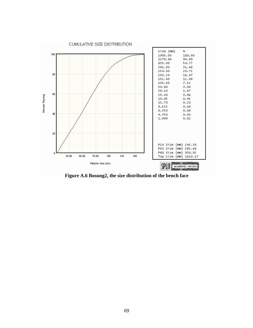
Figure A.6 Bosung2, the size distribution of the bench face
69

Figure A.7 Bosung3, the bench face image
Figure A.8 Bosung3, the analyzed image
70
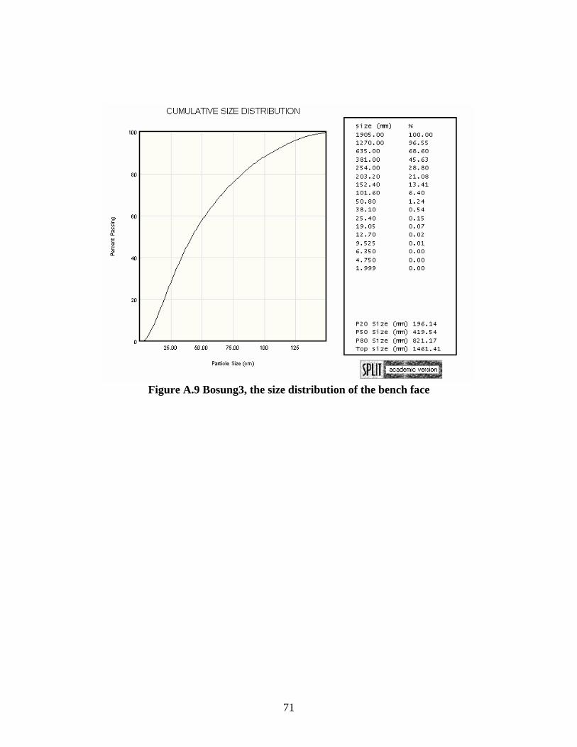
Figure A.9 Bosung3, the size distribution of the bench face
71

Figure A.10 Bosung4, the bench face image
Figure A.11 Bosung4, the analyzed image
72

Figure A.12 Bosung4, the size distribution of the bench face
73

Figure A.13 Bosung5, the bench face image
Figure A.14 Bosung5, the analyzed image
74

Figure A.15 Bosung5, the size distribution of the bench face
75

Figure A.16 Pittsboro, the bench face image
Figure A.17 Pittsboro, the analyzed image
76

Figure A.18 Pittsboro, the size distribution of the bench face
77

Figure A.19 Boxley, the bench face image
Figure A.20 Boxley, the analyzed image
78

Figure A.21 Boxley, the size distribution of the bench face
79

Figure A.22 Sanyang1, the bench face image
Figure A.23 Sanyang1, the analyzed image
80

Figure A.24 Sanyang1, the size distribution of the bench face
81

Figure A.25 Sanyang2, the bench face image
Figure A.26 Sanyang2, the analyzed image
82

Figure A.27 Sanyang2, the size distribution of the bench face
83

Figure A.28 Sanyang3, the bench face image
Figure A.29 Sanyang3, the analyzed image
84

Figure A.30 Sanyang3, the size distribution of the bench face
85

Figure A.31 Sanyang4, the bench face image
Figure A.32 Sanyang4, the analyzed image
86

Figure A.33 Sanyang4, the size distribution of the bench face
87

Figure A.34 Sanyang5, the bench face image
Figure A.35 Sanyang5, the analyzed image
88

Figure A.36 Sanyang5, the size distribution of the bench face
89

APPENDIX B -
Image Analysis of the Muckpile
90

Figure B.1 Bosung1, the muckpile image
Figure B.2 Bosung1, the analyzed image
91

Figure B.3 Bosung1, the size distribution of the muckpile
92

Figure B.4 Bosung2, the muckpile image
Figure B.5 Bosung2, the analyzed image
93

Figure B.6 Bosung2, the size distribution of the muckpile
94

Figure B.7 Bosung3, the muckpile image
Figure B.8 Bosung3, the analyzed image
95

Figure B.9 Bosung3, the size distribution of the muckpile
96

Figure B.10 Bosung4, the muckpile image
Figure B.11 Bosung4, the analyzed image
97

Figure B.12 Bosung4, the size distribution of the muckpile
98
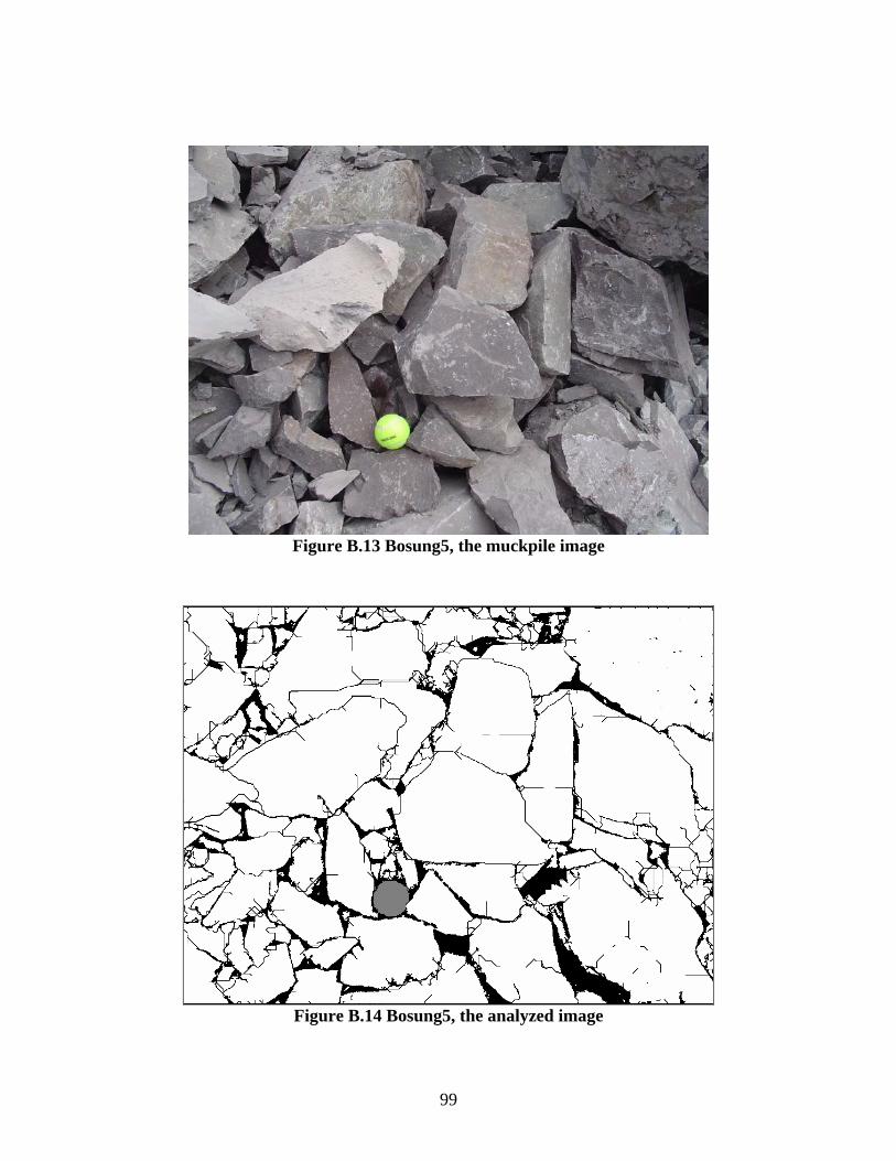
Figure B.13 Bosung5, the muckpile image
Figure B.14 Bosung5, the analyzed image
99

Figure B.15 Bosung5, the size distribution of the muckpile
100

Figure B.16 Pittsboro, the muckpile image
Figure B.17 Pittsboro, the analyzed image
101

Figure B.18 Pittsboro, the size distribution of the muckpile
102

Figure B.19 Boxley, the muckpile image
Figure B.20 Boxley, the analyzed image
103
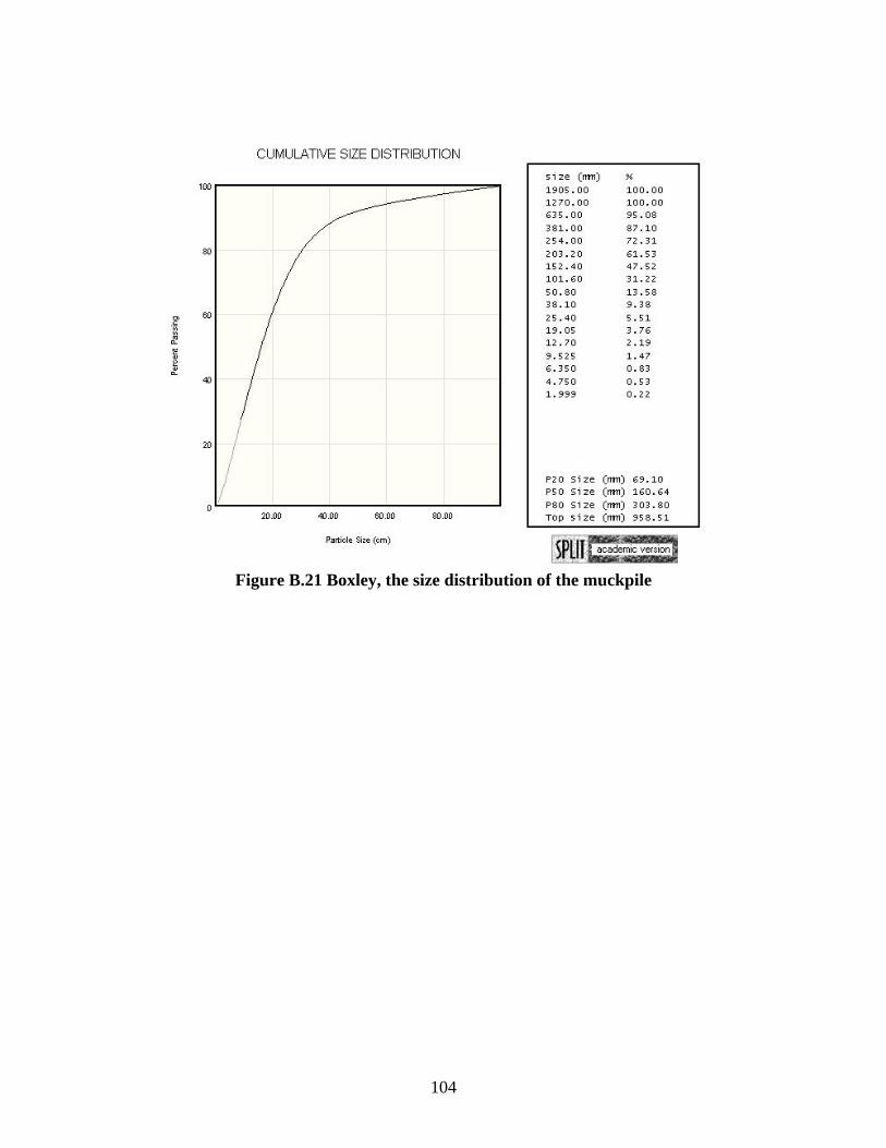
Figure B.21 Boxley, the size distribution of the muckpile
104

Figure B.22 Sanyang1, the muckpile image
Figure B.23 Sanyang1, the analyzed image
105

Figure B.24 Sanyang1, the size distribution of the muckpile
106

Figure B.25 Sanyang2, the muckpile image
Figure B.26 Sanyang2, the analyzed image
107

Figure B.27 Sanyang2, the size distribution of the muckpile
108

Figure B.28 Sanyang3, the muckpile image
Figure B.29 Sanyang3, the analyzed image
109

Figure B.30 Sanyang3, the size distribution of the muckpile
110

Figure B.31 Sanyang4, the muckpile image
Figure B.32 Sanyang4, the analyzed image
111

Figure B.33 Sanyang4, the size distribution of the muckpile
112

Figure B.34 Sanyang5, the muckpile image
Figure B.35 Sanyang5, the analyzed image
113

Figure B.36 Sanyang5, the size distribution of the muckpile
114

APPENDIX C -
Rock tests (Brazilian, Tilt, and KIC Test)
115

Table C.1 Bosung, Mode I fracture toughness, KIC
Sample # Peak Load
Crack Length Thickness Diameter
P-splitting
F-Gregory Kq
Pv, N a, m t, m D, m Psp, N m-1/2 MPa(m1/2)BS-2 1540.7 0.02263 0.02697 0.05423 1075.451 17.148 1.497BS-3 1597.7 0.02276 0.02586 0.05423 1115.247 17.292 1.628BS-4 1594.7 0.02253 0.02593 0.05423 1113.162 17.033 1.604BS-5 1874.6 0.02281 0.03048 0.05425 1308.544 17.334 1.623BS-6 1470.4 0.02258 0.02492 0.05428 1026.368 17.059 1.541BS-7 1756.5 0.02248 0.02944 0.05425 1226.106 16.961 1.552BS-8 1856.7 0.02281 0.03005 0.05423 1296.049 17.350 1.632BS-9 1551.5 0.02263 0.02858 0.05425 1083.008 17.132 1.422
BS-10 1382.7 0.02271 0.02692 0.05425 965.179 17.218 1.349BS-11 1968.5 0.02309 0.02687 0.05423 1374.090 17.675 1.959
Coefficient of Friction,µ 0.580 Wedge Angle, α 0.19198622
Tensile Strength, σt 18.85 Mpa
AVG 1.539STDEV 0.100
Table C.2 Bosung, Size Check for KIC validity Size Check
Sample # a D-a t Value Value Validity Validity Validity Validity m m m D-a, a t a D-a t Overall
BS-2 0.023 0.032 0.027 0.0158 0.0017 OK OK OK OK BS-3 0.023 0.031 0.026 0.0187 0.0020 OK OK OK OK BS-4 0.023 0.032 0.026 0.0181 0.0019 OK OK OK OK BS-5 0.023 0.031 0.030 0.0185 0.0020 OK OK OK OK BS-6 0.023 0.032 0.025 0.0167 0.0018 OK OK OK OK BS-7 0.022 0.032 0.029 0.0169 0.0018 OK OK OK OK BS-8 0.023 0.031 0.030 0.0187 0.0020 OK OK OK OK BS-9 0.023 0.032 0.029 0.0142 0.0015 OK OK OK OK BS-10 0.023 0.032 0.027 0.0128 0.0014 OK OK OK OK BS-11 0.023 0.031 0.027 0.0270 0.0029 NO OK OK NO
Average 0.023 0.032 0.028 0.0167 0.0018 OK OK OK OK
116

Table C.3 Bosung, Brazilian Test Sample ID Diameter(in) Thickness(in) Load(lbs) Tensile Strength(Mpa)
BS-1 2.134 1.040 7566 14.96 BS-2 2.132 1.008 7788 15.91 BS-3 2.133 1.033 7550 15.04 BS-4 2.139 1.076 9834 18.75 BS-5 2.133 1.067 10354 19.97 BS-7 2.130 1.035 8866 17.65 BS-8 2.140 1.012 8024 16.26
Average 16.94
S.D. 1.92
Table C.4 Bosung, Tilt test Sample angle Ave.angle
B-1 31 33 32 32.5 33 32.3 B-2 27 27 28 29 32 28.6 B-3 30 31 32 32.5 35 32.1 B-4 30 27 27 26 27 27.4 B-5 27 32 30 27 34 30
Average 30.1
Friction Coe. 0.58
117

Table C.5 Sanyang, Mode I fracture toughness, KIC
Sample # Peak Load
Crack Length Thickness Diameter
P-splitting
F-Gregory Kq
Pv, N a, m t, m D, m Psp, N m-1/2 MPa(m1/2)S-1 1421.5 0.02248 0.02634 0.05436 1106.972 16.898 1.562S-2 1520.3 0.02283 0.02598 0.05428 1183.911 17.347 1.723S-3 1154.9 0.02248 0.02705 0.05425 899.362 16.961 1.239S-4 1964.7 0.02283 0.02687 0.05425 1529.982 17.363 2.155S-5 1597.1 0.02273 0.02604 0.05428 1243.718 17.231 1.799S-6 2311.4 0.02268 0.02576 0.05428 1799.969 17.173 2.626S-7 1419.9 0.02266 0.02708 0.05425 1105.726 17.161 1.534S-8 2112.7 0.02281 0.02662 0.05428 1645.234 17.318 2.335S-9 1874.6 0.02281 0.02738 0.05431 1459.817 17.301 2.013S-10 1433.7 0.02299 0.02710 0.05428 1116.473 17.523 1.569S-11 1889.2 0.02301 0.02637 0.05425 1471.187 17.569 2.129
Coefficient of Friction,µ 0.514 Wedge Angle, α 0.19198622
Tensile Strength, σt 20.01 Mpa
AVG 1.724STDEV 0.193
Table C.6 Sanyang, Size Check for KIC validity Size Check
Sample # a D-a T Value Value Validity Validity Validity Validity m m M D-a, a t a D-a t Overall
S-1 0.022 0.032 0.026 0.0152 0.0016 OK OK OK OK S-2 0.023 0.031 0.026 0.0185 0.0020 OK OK OK OK S-3 0.022 0.032 0.027 0.0096 0.0010 OK OK OK OK S-4 0.023 0.031 0.027 0.0290 0.0031 NO OK OK NO S-5 0.023 0.032 0.026 0.0202 0.0022 OK OK OK OK S-6 0.023 0.032 0.026 0.0430 0.0046 NO NO OK NO S-7 0.023 0.032 0.027 0.0147 0.0016 OK OK OK OK S-8 0.023 0.031 0.027 0.0340 0.0037 NO NO OK NO S-9 0.023 0.031 0.027 0.0253 0.0027 NO OK OK NO
S-10 0.023 0.031 0.027 0.0154 0.0017 OK OK OK OK S-11 0.023 0.031 0.026 0.0283 0.0030 NO OK OK NO
Average 0.023 0.032 0.027 0.0186 0.0020 OK OK OK OK
118

Table C.7 Sanyang, Brazilian Test
Sample Diameter(in) Thickness(in) Load(lbs) Tensile strength(MPa) S-1 2.133 1.022 7509 15.12 S-2 2.137 0.805 8530 21.76 S-3 2.129 1.000 7404 15.26 S-4 2.131 1.021 8336 16.82 S-5 2.131 1.010 8004 16.32 S-6 2.133 1.064 8538 16.51 S-7 2.135 1.054 10416 20.32
Average 17.45
S.D. 2.57
Table C.8 Sanyang, Tilt test Sample angle Ave.angle
S-1 25 24 25 28 27 25.8 S-2 26 26 29 25 27 26.6 S-3 30 28.5 30 31 31 30.1 S-4 25 32 25 24 27 26.6 S-5 26 28 26 26 29 27
Average 27.2
Friction Coe. 0.514
119

Table C.9 Boxley, Mode I fracture toughness, KIC
Sample # Peak Load
Crack Length Thickness Diameter
P-splitting
F-Gregory Kq
Pv, N a, m t, m D, m Psp, N m-1/2 MPa(m1/2)B-1-1 889.0 0.02032 0.02449 0.05022 760.764 17.035 1.177B-1-2 621.0 0.02123 0.02390 0.05024 531.422 18.158 0.878B-1-3 1103.6 0.02156 0.02682 0.05024 944.408 18.594 1.413B-2-1 1008.8 0.02149 0.02629 0.05024 863.283 18.492 1.313B-2-2 1556.8 0.02129 0.02573 0.05024 1332.235 18.224 2.050B-3-1 1111.2 0.02118 0.02741 0.05019 950.912 18.129 1.369B-3-2 1874.0 0.02136 0.02748 0.05022 1603.680 18.343 2.321B-4-1 1306.0 0.02139 0.02507 0.05022 1117.613 18.376 1.775B-4-2 1432.0 0.02149 0.02687 0.05019 1225.438 18.530 1.826
Coefficient of Friction,µ 0.462 Wedge Angle, α 0.19198622
Tensile Strength, σt 15.95 Mpa
AVG 1.230STDEV 0.216
Table C.10 Boxley, Size Check for KIC validity Size Check
Sample # a D-a t Value Value Validity Validity Validity Validity m m m D-a, a t a D-a t Overall
B-1-1 0.020 0.030 0.024 0.0136 0.0015 OK OK OK OK B-1-2 0.021 0.029 0.024 0.0076 0.0008 OK OK OK OK B-1-3 0.022 0.029 0.027 0.0196 0.0021 OK OK OK OK B-2-1 0.021 0.029 0.026 0.0169 0.0018 OK OK OK OK B-2-2 0.021 0.029 0.026 0.0413 0.0044 NO NO OK NO B-3-1 0.021 0.029 0.027 0.0184 0.0020 OK OK OK OK B-3-2 0.021 0.029 0.027 0.0529 0.0057 NO NO OK NO B-4-1 0.021 0.029 0.025 0.0310 0.0033 NO NO OK NO B-4-2 0.021 0.029 0.027 0.0328 0.0035 NO NO OK NO
Average 0.021 0.029 0.026 0.0149 0.0016 OK OK OK OK
120

Table C.11 Boxley, Brazilian Test Sample Diameter(in) Thickness(in) Load(lbs) Tensile Strength(Mpa) B-2-5 1.977 1.057 7990 16.78 B-2-6 1.977 1.055 6034 12.70 B-2-7 1.977 0.914 6316 15.34 B-1-4 1.976 0.987 6638 14.94 B-1-5 1.975 1.070 7142 14.83 B-1-6 1.976 1.058 7257 15.24 B-3-3 1.977 1.073 6354 13.15 B-3-4 1.976 1.007 6750 14.89 B-4-3 1.975 1.135 6964 13.64 B-4-4 1.977 1.117 7898 15.70
Average 14.72
S.D. 1.23
Table C.12 Boxley, Tilt test Sample angle Ave.angle B-1-7 28 27 26 24.5 25.5 26.2 B-1-8 30.5 33 28.5 27.5 27.5 29.4 B-3-5 23.5 21 25 21.5 22.5 22.7 B-4-5 20 23.5 22.5 21.5 22 21.9 B-2-8 24.5 21.5 24.5 25 24 23.9
Average 24.8
Friction Coe. 0.462
121

Table C.13 Pittsboro, Mode I fracture toughness, KIC
Sample # Peak Load
Crack Length Thickness Diameter
P-splitting
F-Gregory Kq
Pv, N a, m t, m D, m Psp, N m-1/2 MPa(m1/2)PB-3-10 1991.0 0.02108 0.02601 0.05004 1760.324 18.108 2.670PB-3-8 2083.0 0.02083 0.02596 0.05006 1841.665 17.764 2.763PB-2-7 1035.0 0.02096 0.02713 0.05001 915.086 17.963 1.324PB-2-8 1697.6 0.02070 0.02715 0.05001 1500.917 17.640 2.143PB-1-1 1357.0 0.02045 0.02494 0.04968 1199.779 17.550 1.861PB-1-2 1991.0 0.02118 0.02789 0.05022 1760.324 18.111 2.489PB-1-3 1389.0 0.02108 0.02616 0.05019 1228.071 17.998 1.844PB-1-4 2031.0 0.02126 0.02761 0.05006 1795.690 18.322 2.586PB-3-14 1570.0 0.02042 0.02553 0.05004 1388.101 17.276 2.080PB-3-11 1113.0 0.02007 0.02499 0.05004 984.049 16.848 1.481
Coefficient of Friction,µ 0.445 Wedge Angle, α 0.19198622
Tensile Strength, σt 27.18 Mpa
AVG 1.889STDEV 0.398
Table C.14 Pittsboro, Size Check for KIC validity Size Check
Sample # a D-a t Value Value Validity Validity Validity Validity m m m D-a, a t a D-a t Overall
PB-3-10 0.021 0.029 0.026 0.0241 0.0026 NO OK OK NO PB-3-8 0.021 0.029 0.026 0.0258 0.0028 NO OK OK NO PB-2-7 0.021 0.029 0.027 0.0059 0.0006 OK OK OK OK PB-2-8 0.021 0.029 0.027 0.0155 0.0017 OK OK OK OK PB-1-1 0.020 0.029 0.025 0.0117 0.0013 OK OK OK OK PB-1-2 0.021 0.029 0.028 0.0210 0.0023 OK OK OK OK PB-1-3 0.021 0.029 0.026 0.0115 0.0012 OK OK OK OK PB-1-4 0.021 0.029 0.028 0.0226 0.0024 NO OK OK NO PB-3-14 0.020 0.030 0.026 0.0146 0.0016 OK OK OK OK PB-3-11 0.020 0.030 0.025 0.0074 0.0008 OK OK OK OK Average 0.021 0.029 0.026 0.0121 0.0013 OK OK OK OK
122

Table C.15 Pittsboro, Brazilian Test Sample ID Diameter(in) Thickness(in) Load(lbs) Tensile Strength(Mpa) PB-3-21 1.970 1.069 11760 24.51 PB-1-8 1.972 1.186 10580 19.86 PB-1-9 1.978 1.062 6904 14.43 PB-3-15 1.974 1.073 11052 22.90 PB-3-16 1.974 1.057 12318 25.91 PB-3-18 1.970 0.990 12110 27.25
Average 22.48
S.D. 4.7
Table C.16 Pittsboro, Tilt test Sample angle Ave angle PB-1-6 24 29 26 16 27 24.4 PB-3-12 23 26 24 24 22 23.8 PB-2-9 22 22 22 21 24 22.2 PB-3-13 25 22 22 26 24 23.8 PB-1-7 25 24 26 30 23 25.6 PB-2-10 25 24 24 24 25 24.4
Average 24.0
Friction Coe. 0.445
123
APPENDIX D -
Summarized Blasting pattern and ESE
124

125
Blastin
g patter
nPitt
sboro
Boxley
Bosung
1Bosu
ng2Bos
ung3B
osung4
Bosung
5Sany
ang1S
anyang
2San
yang3
Sanyan
g4San
yang5
Unit
Bench H
eight
19.815.5
411.1
11.111.1
11.15.3
14.314.3
8.410.7
11.4m
Burden
4.574.27
33
2.82.9
2.22.5
2.31.9
1.91.8
mSpa
cing4.57
5.492.9
2.93
2.92.2
2.32.1
1.92.0
1.8m
Rock Sp
ecific G
ravity
2.692.73
2.582.58
2.582.58
2.582.49
2.492.49
2.492.49
t/m^3
Hole di
ameter
165165
7676
7676
7676
7676
7676
mmExp
losives
Hydrom
ite4400
Heet30,
Austinit
eExp
losives
amoun
t per ho
le429
259.5(1
55.54,10
3.96)
2020
2020
5.742
3820
1716
kgExp
losives
energy
per gram
863863
and 912
1100
1100
1100
1100
1100
1100
1100
1100
1100
1100K
cal/Kg
Explosi
ves ene
rgy per
hole431
26625.5
925.5
925.5
925.5
97.29
53.73
48.27
25.39
21.75
20.21K
whEse
387268
103103
107107
110268
292336
222210
wh/tonn
e
Table D
.1 Summ
arized b
lasting
pattern
and Ese
New mit
e plus I
IEm
ulite 150
, New A
NFO