Blending images for texturing 3D models

Adam Baumberg

Canon Research Centre Europe The Braccans, London Road

Bracknell Berkshire, RG12 2XH

adamb@cre.canon.co.uk

Abstract

This paper describes a novel system for building seamless texture maps for a surface of arbitrary topology from real images of the object taken with a standard digital camera and uncontrolled lighting.

In our application we wish to take a sparse set of real images of a 3D object, and apply the images to an approximate surface model of the object to generate a high quality textured model. In practice the measured colour and intensity for a surface element observed in different photographic images will not agree. This is due to the interaction between real world lighting effects (such as highlights and specularities) and variations in the camera gain settings as well as registration and surface modelling errors. We describe a new automatic approach that extends a classical 2D image blending technique to a 3D surface, which produces high quality photo-realistic results at a low computational cost.

1 Introduction Our work is motivated by the desire to produce a low-cost, portable 3D scanning

system based on hand-held digital photographs. In this paper we assume that we have an approximate 3D surface model of an object and a number of photographs of the object taken from known camera positions (with known camera parameters). The key contribution of our work is a method for generating a seamlessly textured model from such data in a computationally efficient manner. We do not require any assumptions

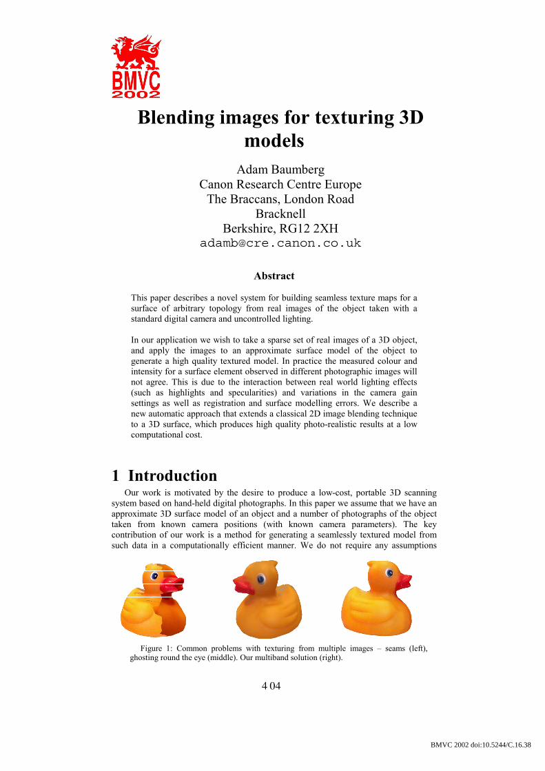
Figure 1: Comghosting round the

mon problems with texturing from multiple images – seams (left), eye (middle). Our multiband solution (right).

404

BMVC 2002 doi:10.5244/C.16.38

about scene lighting or the constancy of camera settings. Hence our method is suitable both for small objects photographed on the desktop as well as larger objects photographed in uncontrolled outdoor environments. Our method avoids the common problems associated with texturing from multiple images shown in Figure 1.

1.1 Related Work Generating 3D models from photographs has received much interest in the

Computer Vision, Photogrammetry and Computer Graphics communities. Much of the research in the Computer Vision community has focused on recovering camera parameters (position, orientation, focal length etc) and surface geometry (3D point data) for example using “structure from motion” [1] or multi-view stereo matching [2].

A common approach for blending image data for texturing is to use a triangle-based scheme [3], [4], [5]. In general these techniques rely on a regular triangular mesh model (with a fairly uniform size and shape for each triangle). Each triangle is assigned to the “best” camera by considering the viewing angle and visibility. A regrouping procedure is applied to minimize the length of the boundaries between regions assigned to different cameras. Blending is restricted to the boundary triangles and simple weighted averaging used to “blur” the seams. This simple technique is quite effective but the size of the “transition” zone between regions textured from different cameras is fixed by the size and shape of the triangles (and hence not suited to irregular meshes). The size of the transition region is crucial. If the triangles are too small the transition region is small and the seams between regions will only be slightly blurred and still visible. If the triangles are large the transition region is too large, which results in blurring away high frequency detail. This can also cause ghosting due to misregistration of the cameras and inaccuracies in the surface model.

Rocchini [4] goes some way to addressing the “ghosting” problem by performing a local triangle based registration at the region bondaries (“frontier faces”). The approach is limited by a simple linear model for local registration, which in practice will only work for a small transition zone. In fact Rocchini concludes that an “increased frontier region or multiresolution approach” is worth future investigation to “handle large chromatic variations between overlapping images” (e.g. due to uncontrolled lighting). Lensch et al [5] address the ghosting problem by optimising the camera registration parameters so as to align the projected texture data on the 3D surface. In their application the 3D surface model is assumed to be highly accurate (e.g. obtained using a hardware laser scanner) whereas we assume only a rough geometric model. Hence we would also need to optimise over the surface shape to eliminate ghosting, which would require optimisation in a very high dimensional space.

An alternative to triangle based schemes is to use per-pixel weighted filtering schemes [2], [9], [10]. For example, Pighin et al describe a system for generating 3D face models from photographs [9]. In this paper a texture blending technique is described for the restricted case of a cylindrical texture map. Cylindrical weight maps are constructed for each camera image that satisfy a number of requirements – visibility (zero weight for hidden surface points), smoothness (the weights should vary smoothly), positional certainty (oblique views have less weight), and optionally view similarity (virtual view dependence). The images are then blended by weighted averaging to produce a view-independent or view dependent texture map. (See [7], [8] for more on view-dependent texture mapping).

More recently, Bernardini et al [10] describe a system for high quality texture reconstruction from multiple 2.5D scans (acquired using a structured light stereo system). Again, a smoothly varying weight function is used to ensure a large transition zone and hence avoid seams. As in [5], an iterative image-based registration method is

405

described to ensure accurate alignment of the scans and minimise ghosting and bluring. The use of calibrated lighting conditions allows the construction of albedo and normal maps. A weighting scheme is then used to blend the albedo and normal texture data.

In our work, we aim to preserve as much image detail as possible to build very high quality view-independent textures. To do this, we have developed a new multi-band 3D “splining” approach to preserve high frequency detail in the transition regions of the surface textures. (The classical 2D image splining approach is described in [6]). We have found that using our multi-band technqiue avoids the requirement to have perfectly aligned texture data. Like Pighin [9], our approach is also based on constructing suitable weight maps. We describe a more general approach for building and utilising weight maps for a surface of arbitrary topology using a camera image-based weight map representation similar to the weighting scheme of Bernardini et al [10]. However, unlike [10] we generate a smooth weight function even for a non-smooth polygonal mesh. We also describe a more general and efficient mechanism for transfering the weight image data into an arbitrary texture domain.

1.2 Generating the input data Our texture generation module requires a 3D surface mesh model of the target object

and a set of input images taken with known camera parameters (intrinsics and extrinsics in the mesh coordinate frame). Like Niem [3] we take a number of photographs of the object we wish to model, placed on a planar calibration object. The calibration object has easily detectable markings that allow us to determine the position and orientation of the camera with respect to the object we wish to model (for details see Taylor et al [11]). A coloured backdrop is used to allow us to segment the object shape to generate a binary silhouette image.

We then approximate the shape of each silhouette with a polygon and back-project to form a 3D cone with the apex at the centre of projection of the camera. The object is constrained to lie in each cone, so we intersect the cones exactly (see Lyons et al [14]) to form an approximation to the object shape (the “visual hull”). The result is an irregular polygonal mesh that we then triangulate using standard methods. Note that there are a large number of alternative 3D reconstruction techniques that could be used as input to our texture blending scheme (e.g. using stereo [2]).

1.3 Texture representation There are many possible ways to represent the texture data for an arbitrary surface.

These range from a single cylindrical texture map (e.g. for faces [9]), to a collection of perspective views of the scene [4], [5], [7].

Our algorithm does not require any specific texture representation. We will assume the surface geometry is stored as a triangular mesh. For each triangle we also store a reference to a texture map image and the 2D texture coordinates for each vertex.

The significant point to note for all mesh-based texture map approaches is that continuity cannot be enforced everywhere. Neighbouring surface elements are not necessarily textured from neighbouring regions in the texture map. This is true even for cylindrical texture maps since the edges of the texture map are spatially separated but represent neighbouring regions on the surface.

Hence we assume that each surface triangle maps to a unique triangle in one of the texture maps but a triangle edge can map to disjoint lines in the texture maps (this is a “seam” in the texture representation). We will need to ensure that these texture representation seams are not visible in the final model by ensuring there is exact agreement on both sides of the seam.

406

triangleof area surfacetriangle projected of area∝w

We have implemented two schemes for representing the surface texture data. The first is a “box” scheme that represents the surface textures using 6 orthographic (non-perspective) “canonical” views of the model (top view, front view etc). For each triangle we texture map using the “best” view for that triangle. This is the canonical view with the highest texture resolution out of all views in which the triangle is completely visible (no occlusion). The benefits of this approach are that it is very simple and the 2D texture coordinates can be calculated implicitly from the 3D vertex data. However for an arbitrary surface we cannot guarantee that every triangle is completely visible in one of the 6 canonical views.

The second scheme is based on [16]. Each triangle is mapped to a right angle triangle and these are packed together in arbitrary positions with a few pixels of padding between the triangles. This scheme ensures that every triangle is fully represented but is not very efficient in terms of compression due to the large number of representation seams (every edge is a seam).

2 Texture “splining” in 3D In this section we describe our approach to blending the texture image data using a

new 3D splining technique.

2.1 General approach The approach we take is to process each camera image sequentially. We generate a

smooth weight function across the surface for each camera which we represent using an image-based representation in the camera image frame. The input camera image data is divided into several frequency bands and each band projected into the texture map representation along with the weight function. We blend each band in the texture map representation separately using different (pixel-wise) filters. The low frequency data is blended using a simple linear averaging filter whereas the high frequency is data with a non-linear (“maximum weight”) filter. Finally, the texture map bands are recombined to generate the final texture map.

In this manner, we avoid convoluted 3D signal processing operations and achieve a comparable result by performing signal processing operations in the camera image frame using the 2D image grid.

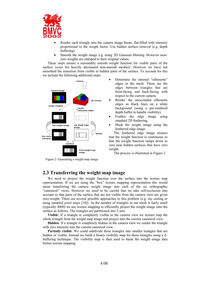
2.2 Building a camera weight function The first step in our algorithm is to build a weight function for each camera. This

weight function will be used to blend the low frequency band texture data using simple weighted averaging as well as providing the basis for the high frequency band filtering.

We adopt the requirements for a cylindrical weight map outlined by Pighin [9] for blending face images on a cylindrical texture map. We note that by construction our weight function will only be non-zero for visible parts of the surface. Hence we can represent the non-zero part of the weight function using a camera image-based representation. We build a greyscale weight image in the camera frame which is then applied to the surface using texture mapping. The weight image is constructed as follows:

• For each triangle calculate a weight factor, w, reflecting the texture resolution using

407

camera

camera image

3D surface

raw weight image

render weights

blur (zero clamped)

raw depth edge image

render silhouette edges

feather

combine

Final weight map image

• Render each triangle into the camera image frame, flat-filled with intensity proportional to the weight factor. Use hidden surface removal (e.g. depth buffering).

• Smooth the weight image e.g. using 2D Gaussian blurring. However near-zero weights are clamped to their original values.

These steps ensure a reasonably smooth weight function for visible parts of the surface (even for heavily decimated non-smooth meshes). However we have not smoothed the transition from visible to hidden parts of the surface. To account for this we include the following additional steps:

• Determine the internal “silhouette” edges in the mesh. These are the edges between triangles that are front-facing and back-facing with respect to the current camera.

• Render the unoccluded silhouette edges as black lines on a white background (using a pre-rendered depth buffer to handle visibility).

• Feather the edge image using standard 2D feathering.

• Mask the weight image using the feathered edge image.

The feathered edge image ensures that the weight function is continuous so that the weight function ramps down to zero near hidden surfaces that have zero weight.

The process is illustrated in Figure 2.

2.3 Transferring the weight map image We need to project the weight function over the surface into the texture map

representation. If we are using the “box” texture mapping representation this would mean transferring the camera weight image into each of the six orthographic “canonical” views. However we need to be careful that we take self-occlusion into account so that parts of the surface that are not visible from the camera view are given zero-weight. There are several possible approaches to this problem (e.g. ray casting or using sampled point maps [10]). As the number of triangles in our mesh is fairly small (typically 4000) we use texture mapping to efficiently project the weight image onto the surface as follows. The triangles are partitioned into 3 sets:

Visible: If a triangle is completely visible in the camera view we texture map the whole triangle from the weight map image and project into the current canonical view.

Hidden: If a triangle is completely hidden in the camera view we render the triangle with zero intensity into the current canonical view.

Partially visible: We could subdivide these triangles into smaller triangles that are hidden or visible. Instead we build a binary visibility map for these triangles using a Z-buffering technique. The visibility map is then used to mask the weight image data before texture mapping.

Figure 2: Generating a weight map image

408

2.4 Multi-band blending in 2D Burt and Adelson describe the “multiresolution spline” for blending two 2D images

whilst preserving as much detail as possible [6]. The basic idea is to decompose each image into frequency bands. A set of low-pass

filters are applied to generate a sequence of images in which the band limit is reduced from image to image. Band-pass images are then obtained by subtracting each low-pass image from the previous image in the sequence. For each frequency band the two band images (obtained from the two input images) are combined (“splined”) using an appropriate weighting function. The weighting function is constructed so that there is smooth transition region of the same size as the image features present in that frequency band. The splined bands can then be summed to generate the final blended image.

This technique allows overlapping images to be combined into a mosaic without introducing noticeable seams between the images whilst still preserving the high frequency details and avoiding noticeable “ghosting”.

2.5 Multi-band blending in 3D We wish to extend the 2D multi-band blending approach to blending images across a

surface in 3D. Ofek et al describe one approach where a variant of conventional 2D splining is described for perspective texture maps [12]. We could apply this kind of approach to the problem for the “box” texture map representation by projecting all the input camera images into each canonical view and perform 2D splining on each canonical view. In practice we have found that this gives rise to noticeable seams between adjacent triangles textured from different canonical views. By treating each canonical view independently we cannot ensure that they are consistent along triangle edges.

Spectral processing of textured surfaces has been described in [13]. A dense sampling of the surface is required and the process of selecting the sample points is computationally expensive (requiring an iterative sample repulsion scheme).

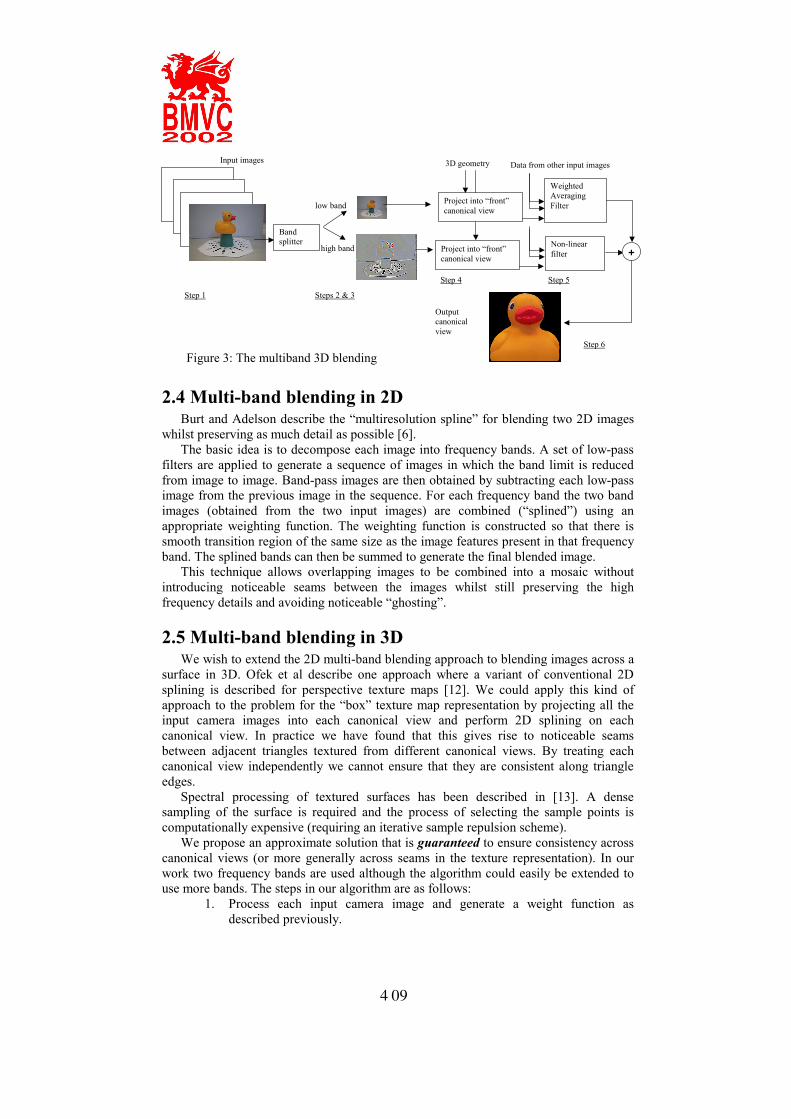
We propose an approximate solution that is guaranteed to ensure consistency across canonical views (or more generally across seams in the texture representation). In our work two frequency bands are used although the algorithm could easily be extended to use more bands. The steps in our algorithm are as follows:

1. Process each input camera image and generate a weight function as described previously.

3D geometry

Band splitter

low band

high band Project into “front”canonical view

Weighted Averaging Filter

Non-linear filter +

Input images

Output canonical view

Figure 3: The multiband 3D blending

Step 1 Steps 2 & 3

Step 4

Project into “front”canonical view

Data from other input images

Step 5

Step 6

409

2. Blur the current camera image to generate a low frequency band camera image using Gaussian blurring.

3. Subtract the original camera image and the low-frequency band image to generate a high frequency band camera image.

4. Project both bands into each canonical view (or more generally into the desired texture map representation) along with the weights.

5. Filter the low-frequency and high frequency texture data independently blending the projected data using pixel-wise operations to ensure consistency. Use a weighted average filter for the low band and a non-linear (“max weight”) filter for the high band.

6. Recombine the filtered texture map bands to generate the final texture maps.

The scheme is illustrated in figure 3. (Note that as the high frequency data is signed we visualise the image by adding a constant so that zero values appear grey).

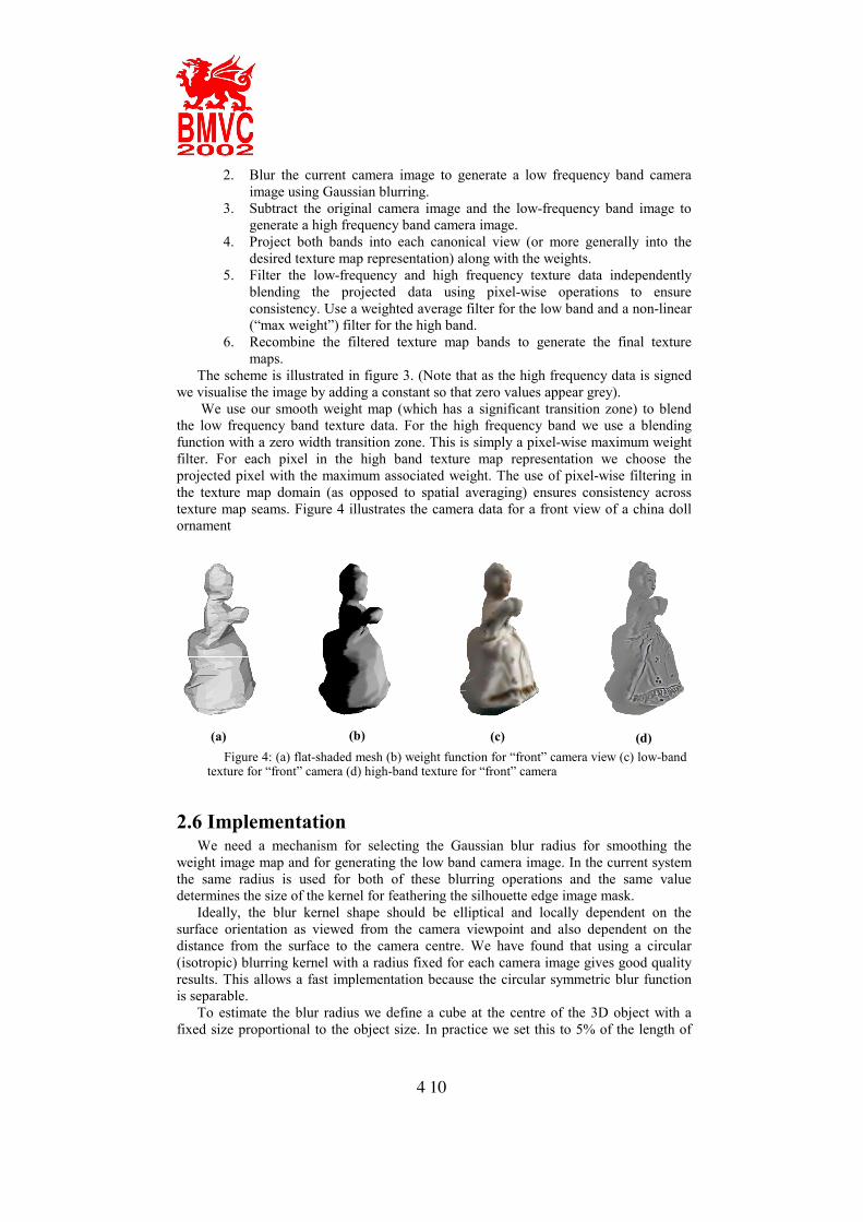
We use our smooth weight map (which has a significant transition zone) to blend the low frequency band texture data. For the high frequency band we use a blending function with a zero width transition zone. This is simply a pixel-wise maximum weight filter. For each pixel in the high band texture map representation we choose the projected pixel with the maximum associated weight. The use of pixel-wise filtering in the texture map domain (as opposed to spatial averaging) ensures consistency across texture map seams. Figure 4 illustrates the camera data for a front view of a china doll ornament

2.6 Implementation We need a mechanism for selecting the Gaussian blur radius for smoothing the

weight image map and for generating the low band camera image. In the current system the same radius is used for both of these blurring operations and the same value determines the size of the kernel for feathering the silhouette edge image mask.

Ideally, the blur kernel shape should be elliptical and locally dependent on the surface orientation as viewed from the camera viewpoint and also dependent on the distance from the surface to the camera centre. We have found that using a circular (isotropic) blurring kernel with a radius fixed for each camera image gives good quality results. This allows a fast implementation because the circular symmetric blur function is separable.

To estimate the blur radius we define a cube at the centre of the 3D object with a fixed size proportional to the object size. In practice we set this to 5% of the length of

(a) (b) (c) (d) Figure 4: (a) flat-shaded mesh (b) weight function for “front” camera view (c) low-band

texture for “front” camera (d) high-band texture for “front” camera

410

the diagonal of the object 3D bounding box. We project the cube primitive into the current camera image and determine the 2D bounding box. We use a blur radius set to the maximum dimension of this 2D bounding box. This approach gives us a value that is consistent across images with different zoom settings but assumes that there is not too much perspective distortion within a single camera view.

3 Results

3.1 Textured models In order to demonstrate our algorithm we used a “doll” test sequence of 16 images

taken of a china doll model using a conventional digital camera. The visual hull model generated contained 4,000 triangles. We also used a further “dino” test sequence of a toy dinosaur with 25 camera images and 10,000 triangles in the mesh model.

We compared the multiband technqiue with two simpler techniques that utilise the same image-based weight maps:

• Averaging – a single band is used and the texture data combined using weighted averaging.

• Best camera – for each texture map pixel the projected camera data with the highest weight is used.

Figures 5 and 6 show the textured mesh for the “china doll” and “dino” input sequences. From these images it is clear that the “averaging” approach suffers from blurring due to camera misregistration and shape modeling errors. The “best camera” method gives crisper textures but suffers from seams due to lighting inconsistencies between input camera images. However, our multiband technique gives a good compromise between these two extremes.

3.2 Performance A sequence of 3 mesh models of the china doll were used to test the dependence on

mesh complexity. The highest resolution mesh has 4000 triangles and we used conventional decimation to generate meshes with 2000 and 1000 triangles. We measured the multiba d texture blending computation time for several typical texture map resolutions (total800Mhz Pentium III p

Figure 5: doll textured using "best camera" approach (left) contains seams, "average" (middle) is slightly blurred and multiband (right) is sharp with no seams.

n

number of pixels in all texture maps). All timings were taken on a rocessor. The results are shown in Table 1.

411

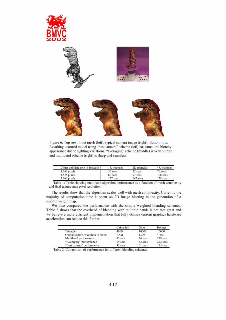
China doll data set (16 images) 1K triangles 2K triangles 4K triangles 1.0M pixels 56 secs 72 secs 76 secs 1.5M pixels 83 secs 97 secs 108 secs 2.0M pixels 127 secs 143 secs 158 secs

Table 1: Table showing multiband algorithm performance as a function of mesh complexity and final texture map pixel resolution.

The results show that the algorithm scales well with mesh complexity. Currently the majority of computation time is spent on 2D image blurring in the generation of a smooth weight map.

We also compared the performance with the simple weighted blending schemes. Table 2 shows that the overhead of blending with multiple bands is not that great and we believe a more efficient implementation that fully utilises current graphics hardware acceleration can reduce this further.

China doll Dino Helmet Triangles 4000 10000 15000 Output texture resolution in pixels 1.5M 1.2M 4.3M Multiband performance 55 secs 74 secs 279 secs “Averaging” performance 39 secs 62 secs 222 secs “Best camera” performance 32 secs 51 secs 175 secs

Table 2: Comparison of performance for different blending schemes

Figure 6: Top row: input mesh (left), typical camera image (right); Bottom row: Resulting textured model using “best camera” scheme (left) has unnatural blotchy appearance due to lighting variations, “averaging” scheme (middle) is very blurred and multiband scheme (right) is sharp and seamless.

412

4 Conclusion We have described a novel system for generating seamless high quality texture maps

from uncontrolled photographs of a surface with known approximate geometry. This system uses a new 3D splining technique that extends conventional 2D splining to the 3D problem where we also need to take account of self-occlusion and visibility issues. Like 2D splining our approach can produce noticeable artefacts where high frequency features such as lines and edges are broken up across regions textured (in the high frequency band) from different misregistered cameras. Future work will address this problem.

In our implementation we have described an efficient image-based representation for defining a smooth camera visibility function over the surface and described how this representation can be used in texture blending applications. We have demonstrated our approach with real examples and shown much improved texture quality compared with two standard techniques (e.g. see Figures 5 and 6). This improved quality does not require significant computational expense and we have shown that high quality results can be generated from 20-25 images in one or two minutes on a standard 800Mhz PC.

Future work will look at extending our approach to more than two frequency bands in a principled manner.

References

[1] R. Hartley and A. Zisserman. Multiple View Geometry in Computer Vision. Cambridge University

Press 2000. [2] Koch R., Pollefeys M. and Van Gool L., “Multi Viewpoint Stereo from Uncalibrated Sequences”,

ECCV ’98, Vol. 1, pp 55-71, Springer. [3] W. Niem. Automatic reconstruction of 3D objects using a mobile camera. Image and Vision Computing

17 (1999) pages 125-134. [4] Rocchini C., Cignoni P. and Montani C., “Multiple textures stitching and blending on 3D objects”, in

Eurographics Rendering Workshop 1999, Eurographics, June 1999 [5] Lensch H., Heidrich W. and Seidel H., “A Silhouette-Based Algorithm for Texture Registration and

Stitching”, Graphical Models Vol 63 No. 4, pp 245-262, Elsevier. [6] P. Burt and E. Adelson. A multiresolution spline with application to image mosaics ACM Transactions

on Graphics (TOG) October 1983 Volume 2 Issue 4. [7] P. Debevec, C. Taylor and J. Malik. Modeling and rendering architecture from photographs: A hybrid

geometry and image-based approach. In conference proceedings ACM SIGGRAPH 96 pages 11-20. [8] Image-based visual hulls Wojciech Matusik , Chris Buehler , Ramesh Raskar , Steven J. Gortler ,

Leonard McMillan Proceedings of the conference on Computer graphics July 2000. [9] Synthesizing realistic facial expressions from photographs Frédéric Pighin , Jamie Hecker , Dani

Lischinski , Richard Szeliski , David H. Salesin Proceedings of the 25th annual conference on Computer Graphics July 1998

[10] F. Bernardini, I. Martin and H. Rushmeier. High Quality Texture Reconstruction from Multiple Scans. IEEE Transactions on Visualization and Computer Graphics volume 7 no. 4. Oct-Dec 2001.

[11] Taylor R., Kirk R., Baumberg A., Lyons A., Davison A. “Image Processing Apparatus” Patent no. WO0139124 ( http://gb.espacenet.com/ )

[12] E. Ofek, E. Shilat and M. Werman. Multiresolution Textures from Image Sequences. IEEE Computer Graphics and Applications volume 17 no.2 pages 18-29, March 1997.

[13] I. Guskov, W. Sweldens and P. Schroder. Multiresolution Signal Processing for Meshes. In conference proceedings ACM SIGGRAPH 99 pages 325-334.

[14] Lyons A., Baumberg A. and Kotcheff A., “SAVANT: A new efficient approach to generating the visual hull”, short paper section Eurographics 2002, Saarbrücken.

[15] M. Eck, T. DeRose, T. Duchamp, H. Hoppe. Multiresolution Analysis of Arbitrary Meshes. In conference proceedings ACM SIGGRAPH 95 pages 173-182.

[16] M. Maruya. Generating a Texture Map from Object-Surface Texture Data. Computer Graphics Forum volume 14 no. 3 1995.

413