blinded assessment of treatment effects utilizing information about the randomization block length

STATISTICS IN MEDICINEStatist. Med. 2009; 28:1690–1706Published online 1 April 2009 in Wiley InterScience(www.interscience.wiley.com) DOI: 10.1002/sim.3576

Blinded assessment of treatment effects utilizing information aboutthe randomization block length

Frank Miller1, Tim Friede2 and Meinhard Kieser3,∗,†

1AstraZeneca, Sodertalje, Sweden2Warwick Medical School, The University of Warwick, U.K.

3Institute of Medical Biometry and Informatics, University of Heidelberg, Germany

SUMMARY

It is essential for the integrity of double-blind clinical trials that during the study course the individualtreatment allocations of the patients as well as the treatment effect remain unknown to any involvedperson. Recently, methods have been proposed for which it was claimed that they would allow reliableestimation of the treatment effect based on blinded data by using information about the block length of therandomization procedure. If this would hold true, it would be difficult to preserve blindness without takingfurther measures. The suggested procedures apply to continuous data. We investigate the properties of thesemethods thoroughly by repeated simulations per scenario. Furthermore, a method for blinded treatmenteffect estimation in case of binary data is proposed, and blinded tests for treatment group differences aredeveloped both for continuous and binary data. We report results of comprehensive simulation studies thatinvestigate the features of these procedures. It is shown that for sample sizes and treatment effects whichare typical in clinical trials, no reliable inference can be made on the treatment group difference whichis due to the bias and imprecision of the blinded estimates. Copyright q 2009 John Wiley & Sons, Ltd.

KEY WORDS: clinical trial; blindness; treatment effect; block randomization; trial integrity

1. INTRODUCTION

One of the most important issues in the design of clinical trials is the implementation of proceduresthat eliminate or minimize bias. Blinding and randomization are generally considered to be themost important techniques in this context [1]. While randomization eliminates bias in treatmentassignment, blinding minimizes the risk of trial personnel or patients being aware of the assignedintervention and thus from being influenced by this. Knowledge of treatment group assignment may,beside others, affect the response of the participants, influence the use of ancillary interventions of

∗Correspondence to: Meinhard Kieser, Institute of Medical Biometry and Informatics, University of Heidelberg,Im Neuenheimer Feld 305, D-69120 Heidelberg, Germany.

†E-mail: [email protected]

Received 28 July 2008Copyright q 2009 John Wiley & Sons, Ltd. Accepted 6 February 2009

BLINDED ASSESSMENT OF TREATMENT EFFECTS 1691

the investigators, or lead to a differential judgment of the outcome by the assessors [2]. But even ifindividual treatment assignments are unknown, knowledge of the size of the treatment effect duringan ongoing trial may influence the attitude of anyone involved in the trial and may thus lead to theoccurrence of bias by mechanisms as such described above. For this reason, regulatory guidelinesstrongly demand that the results of interim analyses are not disseminated to the personnel andpatients involved in a trial [1, 3]. It is therefore standard that any comparison between treatmentgroups that is performed mid-course of a trial is assigned to an independent committee whichmaintains the results strictly confidentially [4]. The only information that is disseminated beyondthe small circle of committee members is whether the trial was stopped or continued. As a furthermeasure, information on who is assigned to which treatment group is not included in the trialdatabase while the study is ongoing but is kept separately with special access rights.

Usually, general information on the implemented randomization procedure is given in theprotocol, such as the method used for random sequence generation or prognostic variables that aretaken into account in stratified randomization. Quite frequently, block randomization is appliedto minimize the risk of obtaining an undesirable sample size imbalance between the treatmentgroups. In order to prevent from the possibility of predicting the assignment of future patientsfrom guessed or known assignments of patients already allocated, it is recommended not to specifythe block length in the protocol [5]. However, trial statisticians are generally aware of the blocklengths and—as they have access to the trial database—they also know the order in which thepatients were recruited. Therefore, they are aware of which patients are in which block. It is evidentthat for extreme outcome scenarios this knowledge can be used to derive information about thetreatment effect even if the individual treatment group allocation remains blinded. For example,in the case of a binary endpoint ‘event yes/no’ where in every block either the event occurs forall patients or does not occur for any patient, it is clear that there is no difference in the treatmenteffect between the groups. The question arises, whether reliable conclusions about the treatmenteffect can be drawn from the blinded data also in more realistic situations. The message given ina recent paper by van der Meulen [6] raises hopes or fears—depending on the perspective—thatthis would be possible. In the abstract of [6] it was claimed that when randomization is done usingpermuted blocks ‘statistical inference of the treatment effects can be conducted’ before unblinding‘yielding consistent and rather precise estimates’ [6, p. 479]. In the light of the above-mentionedfact that the integrity of the trial is questioned if information about the extent of the treatmenteffect becomes known and if actions are taken based on this information during the course of atrial, this would create serious problems.

Other methods that allow a blinded estimation of the treatment effect have been proposed inthe literature before. In the framework of blinded sample size re-estimation, Gould and Shih [7]suggested a method to estimate the within-group variance of normally distributed data. This proce-dure is based on an EM algorithm and does not make use of information about the randomization.It provides not only an estimate of the within-group variance but also of the treatment effect.It was shown that this approach exhibits some major deficits and is not appropriate for sample sizere-estimation based on the blinded variance estimate [8, 9]. Waksman [10] corrected the Gould–Shih procedure such that now the resulting estimates converge to the maximum likelihood (ML)estimates. He investigated the characteristics of the resolved method in a thorough simulationstudy and found that for sample sizes and treatment effects that usually occur in clinical trials, theestimates of the treatment group difference are not accurate enough to be of practical value. Thesame conclusion was drawn by Xing and Ganju [11] for the procedure they derived by making useof the knowledge of the randomization block length. Their primary focus was the construction of a

Copyright q 2009 John Wiley & Sons, Ltd. Statist. Med. 2009; 28:1690–1706DOI: 10.1002/sim

1692 F. MILLER, T. FRIEDE AND M. KIESER

blinded variance estimator for the purpose of blinded sample size re-estimation in case of contin-uous data. They briefly mention that a blinded estimator of the treatment effect can be obtainedas a by-product, based on the difference between the pooled one-sample variance estimator for alldata and their blinded within-group variance estimator (which is a multiple of the variance of theblock means). Based on heuristic arguments and simulation results, Xing and Ganju concludedthat ‘there is no risk of unblinding the trial’ because ‘the variation in the estimate of �2 is largeenough to be practically useless’. In contrast to the other references mentioned above, van derMeulen [6] focuses on estimation of the treatment effect using estimators based on all availableeffect information in the blinded data. Interestingly, he derived blinded moment and ML estimatorsof the treatment group difference for continuous data that use the knowledge of the block lengthapplied in randomization. His work on the estimators is therefore a good basis to investigate theamount of effect-information contained in blinded data. Besides, van der Meulen’s [6] investi-gations suggest that the blinded estimates of the variance he derived with the ML method aremore precise than the blinded treatment effect estimates. Recently, Ganju and Xing [12] discussedspecifically the blinded treatment effect estimation of van der Meulen and concluded that ‘theblinded method is refined enough for blinded variance estimation but blunt enough for inferringefficacy’.

The aim of our paper is to assess the risk of unblinding the treatment effect from blindedinference. This goal is examined (i) by investigating the procedure proposed by van der Meulen forcontinuous data more thoroughly by simulation studies; (ii) by developing alternative approachesfor a blinded assessment of treatment effects by utilizing knowledge of the randomization blocklength in case of continuous and binary outcomes; and (iii) by investigating comprehensively thecharacteristics of the new methods. Thereby, previous work on blinded estimation of treatmentgroup differences is extended in various ways. Section 2.1 takes a closer look at the characteristicsof the procedure proposed by van der Meulen for blinded estimation of treatment effects in caseof continuous data by presenting results of repeated simulations. In Section 2.2, a blinded testfor difference of means is derived and its properties are investigated. An example illustrates thefindings in Section 3. Related methods for binary data did not exist up to now. Section 4 presentsblinded estimators of and a test for treatment group difference in case of binary outcomes andshows their characteristics. We summarize the findings in Section 5 and discuss them in the contextof the literature.

2. BLINDED ASSESSMENT OF TREATMENT EFFECTS FOR CONTINUOUS DATA

2.1. Blinded estimation of treatment effects

Here and in the remainder of the paper the treatment effect, i.e. the difference of the expectedvalues in the two intervention groups, is denoted by �. Hence, in case of continuous data �=�1−�2 with group expectations �1,�2. We start with a block length of l=2 and adopt thenotation used in Reference [6]. Let Yi1, Yi2 denote the first and second observation in blocki , i=1, . . . ,k, where var(Yi j )=�2, i=1, . . . ,k, j =1,2. Further, Z1i =Yi1−Yi2 is the within-block difference in block i and Z2i =Yi1+Yi2 the within-block sum in block i , i=1, . . . ,k;Z2i/2 is therefore the mean in block i . The between-block variation (i.e. the variance of blockmeans) can thus be expressed as S2BB=(1/(k−1))

∑ki=1(Z2i/2− Z2•/2)2, where Z2• denotes

the mean of Z2i , i=1, . . . ,k. Obviously, the expectation of S2BB is given by E(S2BB)=�2/2. The



within-block variation is given by S2WB=(1/k)∑k

i=1 Z21i/2 and has expectation E(S2WB)=�2+

�2/2. Consequently, an unbiased estimator of �2 is given by 2S2WB−4S2BB, and the absolute value

|�| of � can be estimated by√max(2S2WB−4S2BB,0). This is the moment estimator |�| of |�|

presented in [6]. No assumptions are to be made regarding the distribution of the observationswhen deriving this estimator. Alternatively, the ML estimator |�| of |�| can be derived under theassumption of normally distributed observations Yi j . The log likelihood is then given by

l(�1,�2,�2)=

k∑i=1

log

(1

2�(yi1;�1,�2)�(yi2;�2,�2)+

1

2�(yi1;�2,�2)�(yi2;�1,�2)

)where �(y;�,�2) is the density of a normal distribution with mean � and variance �2 [6]. The MLestimates can be obtained by maximizing the log likelihood using the Newton–Raphson algorithm,as, for example, implemented in the SAS/IML function nlpnra. The moment estimators for|�|, �=(1/2)(�1+�2) and �2 can be used to initialize the algorithm. Analogously, the momentestimator and the ML estimator of |�| can be derived for a block length of l=4 (see [6, p. 483]and Appendix A for a correction of the moment estimator given in [6]).

Figures 1 and 2 show the simulated bias |�|−|�| of the moment estimator and the ML estimator|�| for |�| for block lengths of l=2 and l=4, respectively. Considered were (standardized)treatment effects �=0,0.25,0.5 and 1.0 (�=1) and total sample sizes 20, 40, . . . , 100, 200, . . . ,800, 1000 which were balanced between the two groups. It should be noted that total sample sizesof 506, 128 and 34 are required to achieve a power of 80 per cent at one-sided level �=0.025with the unblinded t-test for standardized differences of �/�=0.25, 0.5 and 1.0, respectively. Foreach situation, 1000 simulations were performed.

Both the moment estimator and the ML estimator overestimate the absolute value of the treatmenteffect for �=0 and 0.25 for all sample sizes, while underestimation occurs for �=1 (with theonly exception of l=4 and total sample sizes smaller than 40). As could be expected, the extentof bias is for the same sample sizes generally higher for block size l=4 than for block size 2.For �=0.5, a positive bias is observed for small sample sizes which changes to a negative biaswhen the sample size is increased. The shift from overestimation to underestimation occurs forhigher sample sizes for block size l=4 as compared with l=2. In all considered situations, themean estimates resulting from the moment estimator are slightly smaller than those for the MLestimator, but the difference is negligible for practical purposes. For �>0, the bias approacheszero only for sample sizes which would have been used if the relevant effect assumed at theplanning stage was much smaller than the true treatment effect �. As a reviewer noted, this resultis also reflected in Table I of van der Meulen’s paper [6]: For the data set he used, the treatmenteffect is estimated precisely from blinded data only when the trial has extremely high power (>99per cent); see also [12].

The simulations also show that the standard deviations of the two blinded estimators are verysimilar as well. The variability is higher for block size l=4 as compared with l=2. In comparisonwith unblinded estimation of the treatment effect, the standard deviation of the blinded estimatesis considerably higher by a factor of up to 3 for the range of investigated parameter constellations(results not shown).

What do these results mean in terms of information about the treatment effect that can be inferredfrom blinded data of an ongoing trial? For example, if a clinical trial is powered for 1−�=0.80at a clinically relevant treatment effect of �∗ =0.25, this requires a total sample size of n∗ =506



Figure 1. Mean simulated bias of the blinded treatment effect estimates for block length l=2 in case ofnormally distributed data depending on the true treatment effect �(�=1) and the total sample size n used

for estimation (solid line: blinded ML estimator, dotted line: blinded moment estimator).

(balanced groups, t-test at one-sided level �=0.025). If block randomization with a block size 2is applied and the treatment effect is estimated by the application of the blinded moment or MLestimator based on the data of 500 patients utilizing the information l=2, then Figure 1 showsthat the expected estimated treatment group difference amounts to about 0.27 if the true treatmenteffect is in fact �=0.25. However, if there is actually no treatment group difference at all (�=0),



Figure 2. Mean simulated bias of the blinded treatment effect estimates for block length l=4 in case ofnormally distributed data depending on the true treatment effect �(�=1) and the total sample size n used

for estimation (solid line: blinded ML estimator, dotted line: blinded moment estimator).

the expected blinded estimate is about 0.21. It is therefore evident that in this situation one isnot able to distinguish whether a blinded estimate of, say, 0.25 arises from overestimation of anon-existing treatment group difference or from a treatment effect �>0.



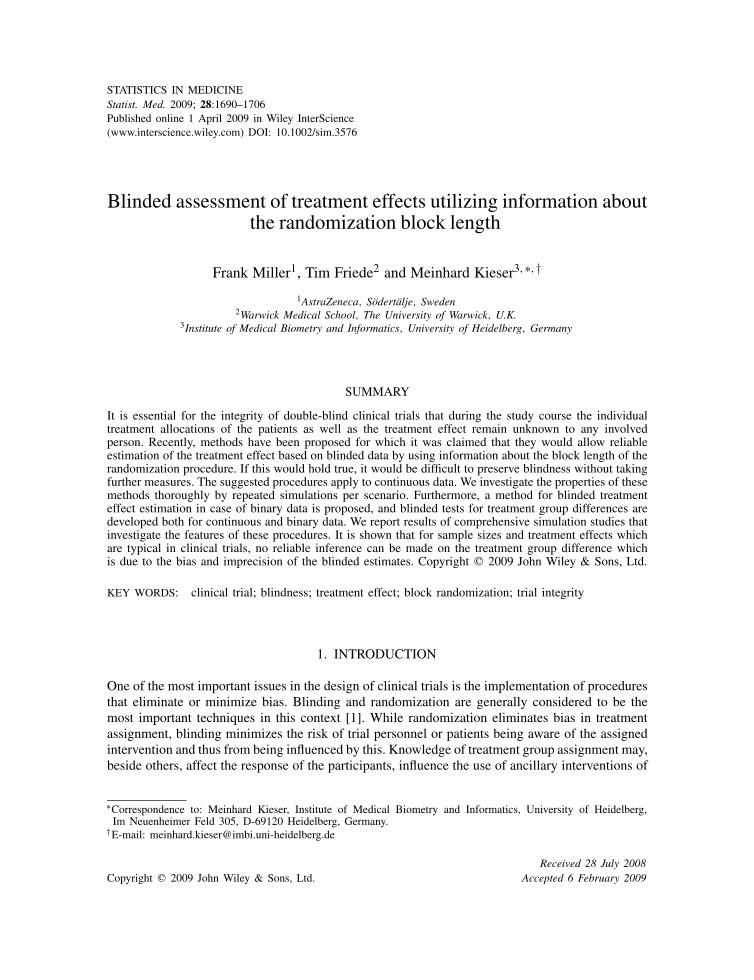
Figure 3 considers this aspect in more detail. The box–whisker plots show for block lengthsl=2 and 4 the range of the central 90 per cent of values arising from 1000 simulated blindedtreatment effect estimates (moment estimator grey, ML estimator white). It can be seen that thereis a heavy overlap of the distributions of the blinded estimators that originate from differentvalues of �. Furthermore, with the exception of the constellations of a total sample size of 500and l=2,�=0.75,1 and l=4,�=1, the box–whisker plot includes the value zero. Hence, foradequately powered studies a blinded estimate of zero gives no indication at all about the actualunderlying treatment effect. The other way round, for �=0 and l=2 (l=4) the upper whiskerreaches the value 1.25, 1.0, and 0.65 (1.5, 1.25, and 0.85) and total sample sizes of 40, 100,and 500, respectively. This means that only huge treatment effect estimates would give causeto the suspicion of a non-zero treatment effect. Figure 3 shows that such estimates occur withconsiderable probability only for at least as extreme true treatment effects. As a consequence,for treatment group differences and sample sizes which are common in clinical trials, a differ-entiation between various extents of � based on the blinded moment or ML estimator is notpossible. This uncertainty about the actual amount of � is a consequence of the substantial posi-tive bias of the blinded estimators for the situation �=0 combined with a high variability of theestimates.

In order to study the sensitivity of our findings to deviations from the normal distributionwe conducted simulations with non-normal distributions including distributions with heavy tails(t-distributions with small number of degrees of freedom) and skewed distributions (e.g. log normaldistribution). We found that the results for the moment estimator are robust against such deviations.However, the ML estimator was sensitive to deviations from normality as expected with at timessevere downwards bias in estimation of the treatment effect �. The general observation for non-normal distributions was that the performance of the blinded estimators is not better as seen fornormal data. A differentiation between various extents of � based on the blinded moment or MLestimator is even more difficult.

2.2. Blinded tests for treatment effect

From the above mentioned formulae for the within-block variation and the between-block variation,a blinded F-test can be derived. As the F-test and the moment estimator are closely related, itcannot be expected that this test will be more revealing than the findings presented in Section 2.1,but is an alternative way to look at this problem. For block length l=2 the test statistics is given by

Fblind,l=2= S2WB

S2BB=

2 · 1k

∑ki=1 Z

21,i

1

k−1

∑ki=1(Z2,i − Z2•)2

and follows the non-central F-distribution Fk,k−1(k�2/(2�2)) with (k,k−1) degrees of freedomand non-centrality parameter k�2/(2�2). Analogously, a test statistics Fblind,l=4 for a blinded F-test can be derived for block length four, which is given in Appendix A. Fblind,l=4 can again beinterpreted as the ratio of the within-block variation to the between-block variation and follows thenon-central F-distribution F3k,k−1(k�2/�2). Owing to the known distribution of the test statistics,the power properties of the blinded F-tests can be evaluated analytically.

Figure 4 shows the relationship between the treatment effect �∗ used for sample size calcu-lation and the ratio r of the true treatment effect � to the effect �∗ that is required to achieve a



Figure 3. Box–whisker plot of the simulated distributions of the blinded estimates |�| of the absolutevalue of the treatment effect |�| in case of normally distributed data depending on the true treatmenteffect �(�=1) and the total sample size n used for estimation (white: blinded ML estimator, grey: blindedmoment estimator; in the box–whisker plot, bottom and top of the boxes are located at the first and thirdquartile, respectively, the central horizontal line marks the median, and 5 and 95 per cent quantile are

indicated by the ends of the whiskers).



Figure 4. Ratio r of the true treatment effect � to the assumed effect �∗ that is required toachieve a power of 1−�=0.50 and 0.80, respectively, for the blinded F-test. The sample sizeis chosen such that the unblinded two-sided t-test at �=0.05 has a power of 80 per cent at the

assumed treatment effect �∗(�=1).

power of 1−�=0.5 and 0.8, respectively, for the blinded F-test with significance level �=0.05.The sample size is chosen such that the unblinded two-sided t-test at �=0.05 has a powerof 1−�∗ =0.8 at the treatment effect �∗(�=1). This means that r is determined such that1−Probf(l−1)k,k−1,nc( f(l−1)k,k−1,1−�)=1−�, where k is the nearest integer to (4/ l)(z1−�/2+z1−�∗)2(�/�∗)2 and nc=r2 ·(z1−�/2+z1−�∗)2. Probfd f1,d f2,ϑ denotes the distribution function ofthe non-central F distribution with (d f1,d f2) degrees of freedom and non-centrality parameterϑ, fd f1,d f2,� is the � quantile of the central F distribution with the same degrees of freedom, andz� is the � quantile of the standard normal distribution.

For l=2 (l=4) and a clinically relevant treatment effect �∗ =0.25 assumed for sample sizecalculation, a 2.7 (3.7) times larger true treatment effect � is necessary to achieve a 50 per centpower for the blinded F-test. A factor of about 3.4 (4.6) between the actual treatment effect andthe effect used for sample size calculation is required to have an adequate power of 80 per cent.From another perspective, if �=�∗ =0.25 the factor between the chosen and the required samplesize amounts to about 46 (136) for a desired power of 50 per cent of the blinded F-test and toabout 104 (309) for 80 per cent. For a clinically relevant treatment effect of �∗ =0.5 the situationbecomes a little bit less extreme. However, still about double (2.8 times) this treatment effect isnecessary to achieve a power of 50 per cent for the blinded F-test, and the true effect needs tobe about 2.6 (3.7) times as large as this effect to get a power of 80 per cent for the blinded test.



In other words, for �=�∗ =0.5 the total sample size required to achieve 80 per cent power for theblinded F-test amounts to about n=3560 (n=10340) while the chosen sample size is n∗ =128.

In practice, one would usually try to learn from the blinded data while the study is still ongoing.Hence, the blinded test would be applied before the data of all n∗ patients are available. As aconsequence, the required factors by which the true effect has to exceed the one used for samplesize calculation to achieve a power of 50 or 80 per cent for the blinded test are even higher asthose reported above.

These considerations show that the blinded F-test has reasonable power only when the truetreatment effect is several times larger than the clinically relevant effect assumed in the samplesize calculation of the study, i.e. if the study is an overpowered study from a retrospective point ofview. Though there is a possibility for this to happen, this is a very rare event in clinical practice.

3. EXAMPLE

In order to illustrate the results, we consider placebo-controlled clinical studies in the acute treat-ment of major depression. The change in total score of the Hamilton Rating Scale for Depression(HAM-D, 17-item version) [13] between baseline and end of therapy is often used as the primaryendpoint in such studies, and a difference of �∗ =3 points can be considered as clinically rele-vant [14]. If the standard deviation � is assumed to lie within the range of 5–8 as usually observedfor this outcome (see, for example, Reference [15]). This corresponds to total sample sizes of90–230 required to achieve a power of 80 per cent for the treatment group difference �∗ =3 (two-sided t-test, �=0.05). These sample sizes match well the number of patients typically included instudies investigating the efficacy of the treatment of acute major depression (see, for example, thesystematic reviews [15, 16]).

The true treatment group difference needed to achieve a power of 1−�=0.80 for the blindedF-test would amount to 7.4 (�=5) or 8.8 (�=8) HAM-D points, respectively, for block length twoand 10.5 (�=5) or 11.9 (�=8), respectively, for block length four. For all existing antidepressants,such huge overall treatment effects are out of reach. The other way round, if the true treatmenteffect would amount to �=3 HAM-D points, the sample size required to attain a power of1−�=0.80 for the blinded F-test would be 1800 (�=5) or 10 700 (�=8), respectively, for blocklength two, and 5200 (�=5) or 31 500 (�=8), respectively, for block length four. However, thereis no reason to perform such large-scale placebo-controlled studies investigating the efficacy ofshort-term treatment of major depression.

In a double-blind, placebo-controlled trial Kalb et al. [17] investigate the efficacy of St. John’swort in patients with mild to moderate depression. The primary variable was the change inHAM-D total score between baseline and end of the six weeks acute treatment phase. Owing tothe uncertainty about the variability of the primary endpoint and the expected treatment effect,the study was planned with an interim analysis that should be performed when roughly half ofthe projected sample size of 130 was achieved. A block length of two was used for randomization.For those 72 patients that were included in the interim analysis, 35 blocks were complete suchthat a blinded assessment could be based on 70 patients. Applying the blinded ML- and momentestimator to this data set leads to estimated treatment effects of 3.2 and 2.4 points, respectively.Employing the one-sample estimator of the standard deviation of 6.3 results in an estimatedstandardized treatment effect of 0.4–0.5. In view of the results shown in Figure 3, this estimate iscompatible with true treatment effects from 0.0 to 1.0. Application of the blinded F-test leads to



a test statistic of F=1.08, which corresponds to a p-value of p=0.42. Hence, blinded estimationand testing give no hint for a significant difference between the two treatment groups. However,the unblinded estimate of the difference between the group means amounts for the same data setto 5.1 and the two-sample t-test results in a two-sided p-value of p=0.0004. As a consequence,the study could be stopped after the planned interim analysis with a significant superiority of St.John’s wort to placebo (pre-defined critical boundary for early rejection �1=0.0207), whereas theblinded methods would not have given any indication to complete the trial early. Therefore, thisreal study data give another counter-example to the claim that blinded inference ‘takes away theneed of conducting interim analyses’ [6].

4. BLINDED ASSESSMENT OF TREATMENT EFFECTS FOR BINARY DATA

4.1. Blinded estimation of treatment effects

In case of binary data, we consider the ML estimator and the moment estimator for blindedestimation of the treatment effect. We will see that this approach leads to a simple expression forthe estimator. In order to avoid repetition we restrict the presentation here to block length l=2as in this situation most information can be drawn from the blinded data thus being the best casescenario for the performance of blinded estimation methods.

The information included in blinded binary data is the number of events that occurred in eachblock and the order they occurred. In the case of block size l=2, the numbers a0,a10,a01,a2 ofblocks with 0 events, with one event that occurs for the first patient, with one event that occursfor the second patient and with two events, respectively, can be observed. If a10 or a01 is ‘large’,one would become suspicious that there may be a difference between the treatment groups. Incontrast, for every block with no event or two events one knows for sure that there is no differencebetween the number of events between the treatment groups.

The blinded ML estimator for the difference in event rates between the two treatments can bederived analytically. If pi denotes the true event rate in treatment group i=1,2, the probabilities ofobserving a block with 0, 2, or 1 event are (1− p1)(1− p2), p1 p2, and 1−(1− p1)(1− p2)− p1 p2,respectively. The probabilities to observe a block with one event that occurs in the first patientor a block with one event that occurs in the second patient are equal. Hence, the likelihoodfunction is given by [(1− p1)(1− p2)]a0[p1 p2]a2[(1−(1− p1)(1− p2)− p1 p2)/2]a10+a01 . We canrestrict on using the total number of blocks with one event a1=a10+a01 instead of (a10,a01),since the likelihood function shows that (a0,a1,a2) is a sufficient statistic. If the expression aboveis re-parameterized with �=(p1+ p2)/2,q=(p1− p2)/2, and d=q2, it can be seen after somecalculation that the log likelihood is maximized for �=(a1+2a2)/(2k) (which is the observedoverall event rate) and for d=(a21−4a0a2)/(2k)2 if (a21−4a0a2)/(2k)2�0, and d=0 otherwise.Hence, the blinded ML estimator for |�|=|p1− p2|=2

√d in case of block length l=2 is given

by |�|=(1/k)√max(a21−4a0a2,0).

Another possibility is to apply the moment estimator presented in Section 2.1 directly to binarydata. In case of binary data and block length l=2 we find S2WB=a1/(2k) and S2BB=(a0�

2+a1(�−0.5)2+a2(1− �)2)/(k−1). With these expressions, the moment estimator

√max(2S2WB−4S2BB,0)

for |�|=|p1− p2| can be calculated.



Figure 5 shows the box–whisker plots covering the central 90 per cent of the empirical distribu-tion of the blinded estimates for l=2 (moment estimator grey, ML estimator white) arising from1000 simulations for each situation. Overall rates �=(p1+ p2)/2 of 0.2, 0.5, treatment effects�= p1− p2 of 0,0.05, . . . ,0.3 and balanced total sample sizes of 100, 500 and 1000 were consid-ered. Qualitatively, the results are very similar to those obtained for continuous data. Again thebox–whisker plots show an extensive overlap for different values of � and �. Moreover, they coverthe value zero for almost all considered situations with the exception of some combinations of atotal sample size of 500 or 1000 and treatment effects of 0.25 or 0.3. However, in these situationthe total sample size required to achieve a power of 80 per cent with the unblinded chi-square testis much lower and ranges from 54 (�=0.2,�=0.3) to 86 (�=0.5,�=0.3). Hence, for reasonablypowered studies a blinded estimate of zero for the treatment group difference is both in accordancewith the assumption �=0 and �>0. As for continuous data, the upper whiskers reach very largetreatment effects for �=0, for example, values of 0.50, 0.32, and 0.27 for an overall rate of�=0.5 and total sample sizes of 100, 500, and 1000, respectively. Therefore, only if even moreextreme values are obtained from blinded estimation of the group difference it is worth to speculatewhether the true treatment effect might be different from zero. However, such large estimatedeffects occur in turn only for very large true differences with noticeable probability. In summary,it can be concluded that for treatment effects and sample sizes which are usually met in clinicaltrials different values of � cannot be distinguished by blinded moment or ML estimation.

4.2. Blinded tests for treatment effect

In Section 2.2 we introduced the F-test Fblind,l=2= S2WB/S2BB for continuous data that we couldapply for binary data as well. In case of binary data and block length l=2 we can employ theexpressions for S2WB and S2BB given in the previous section. Unlike with normal data, however,the reference distribution is not an F-distribution. One way of obtaining a reference distributionis by considering all permutations of ‘1’ (event) and ‘0’ (no event) keeping the total number ofevents fixed. It can be shown that the between-block variation S2BB is invariant to permutations.Therefore, the test statistics reduces to a1 after elimination of invariants, with larger values of a1being stronger evidence against the null hypothesis of no effect. A p-value for the test is given by

floor(e/2)∑b2=max{0,e−k}

(k

b2

)(k−b2

b1

)2b1 I{b1�a1}

where floor(x) is the largest integer that is less than or equal to x,e=2a2+a1,b1=b1(b2)=e−2b2,and I{·} denotes the indicator function.

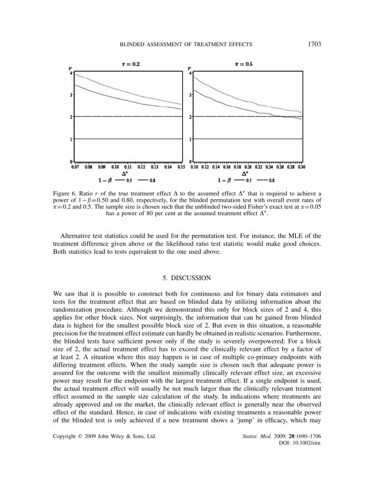
Similar to Figure 4 in Section 2.2, Figure 6 shows the relationship between the risk difference�∗ used for sample size calculation and the ratio r of the actual risk difference � to the effect �∗that is required to achieve a power of 1−�=0.5 and 0.8, respectively, for the blinded permutationtest given above with an overall event rate of �=0.2 and 0.5. Using the approximation formulagiven in [18] the sample size is calculated such that the unblinded two-sided Fisher’s exact test hasa power of 1−�∗ =0.8 for level �=0.05, overall event rate �=0.2,0.5, and difference in eventrates �∗. The ratios r were determined by means of line searches over � with step size 0.005.Hereby the power values of the blinded test were simulated using 50 000 replications.

As can be seen from Figure 6 the risk differences need to be 2–4 times larger than anticipatedin order to obtain a power in the range of 0.5 to 0.8 for the considered combinations of ratedifferences and overall event rates. This is in keeping with similar effects observed in Figure 4.



Figure 5. Box–whisker plot of the simulated distributions of the blinded estimates |�| of the absolute valueof the treatment effect |�| in case of binary data depending on the true treatment effect �, the overallevent rate � and the total sample size n used for estimation (white: blinded ML estimator, grey: blindedmoment estimator; in the box–whisker plot, bottom and top of the boxes are located at the first and thirdquartile, respectively, the central horizontal line marks the median, and 5 and 95 per cent quantile are

indicated by the ends of the whiskers).



Figure 6. Ratio r of the true treatment effect � to the assumed effect �∗ that is required to achieve apower of 1−�=0.50 and 0.80, respectively, for the blinded permutation test with overall event rates of�=0.2 and 0.5. The sample size is chosen such that the unblinded two-sided Fisher’s exact test at �=0.05

has a power of 80 per cent at the assumed treatment effect �∗.

Alternative test statistics could be used for the permutation test. For instance, the MLE of thetreatment difference given above or the likelihood ratio test statistic would make good choices.Both statistics lead to tests equivalent to the one used above.

5. DISCUSSION

We saw that it is possible to construct both for continuous and for binary data estimators andtests for the treatment effect that are based on blinded data by utilizing information about therandomization procedure. Although we demonstrated this only for block sizes of 2 and 4, thisapplies for other block sizes. Not surprisingly, the information that can be gained from blindeddata is highest for the smallest possible block size of 2. But even in this situation, a reasonableprecision for the treatment effect estimate can hardly be obtained in realistic scenarios. Furthermore,the blinded tests have sufficient power only if the study is severely overpowered: For a blocksize of 2, the actual treatment effect has to exceed the clinically relevant effect by a factor ofat least 2. A situation where this may happen is in case of multiple co-primary endpoints withdiffering treatment effects. When the study sample size is chosen such that adequate power isassured for the outcome with the smallest minimally clinically relevant effect size, an excessivepower may result for the endpoint with the largest treatment effect. If a single endpoint is used,the actual treatment effect will usually be not much larger than the clinically relevant treatmenteffect assumed in the sample size calculation of the study. In indications where treatments arealready approved and on the market, the clinically relevant effect is generally near the observedeffect of the standard. Hence, in case of indications with existing treatments a reasonable powerof the blinded test is only achieved if a new treatment shows a ‘jump’ in efficacy, which may



happen only in exceptional circumstances in drug development. Consequently, the only realisticsituations where reliable information about the treatment effect can be gained from blinded datain case of an overpowered study are in trials which are performed with common treatments but innew populations, or in indications where no efficacious treatment exists up to now. Especially,in these situations, adequate measures should be taken to exclude the use of blinded data forinference about the treatment effect. First of all, the use of alternative randomization techniquesto block randomization (see, e.g. [19]) could be considered. If block randomization is used theblock length should be chosen not too small. Fixed small block lengths are often used to avoidimbalances in patient numbers between the intervention groups, for example, if randomization isstratified by centres with small sample sizes per centre. The results of our investigations add tothe known disadvantages of this practice [20] and should be carefully weighted against its meritsbefore application. Second, details about the randomization procedure should not be described inthe protocol but specified in a separate document that is withheld from all persons involved in thestudy. Furthermore, the process of generating the allocation sequence should be separated from thepersonnel that has access to the trial database. By this, it can definitely be avoided that knowledgeabout the randomization scheme is used to derive information about the treatment effect from theblinded study data by application of the methods described above.

In case of a reasonable possibility of an overpowered study, the introduction of an interimanalysis that allows for early stopping in case of overwhelming efficacy might be an option inaddition to the measures mentioned above. This is a much more efficient way of conducting thetrial than trying to recover treatment effect estimates from blinded data.

In summary, for all proposed approaches for blinded assessment of the treatment effect it holdstrue what Waksman states on the corrected EM algorithm-based method, namely ‘it is interestingto note that the procedure can accurately and precisely estimate the difference when either thesample size or the true difference is sufficiently large’ [10]. However, and this is the reassuringmessage: for combinations of sample sizes and treatment effects which are typical in clinical trials,no reliable inference can be made on the treatment group difference due to the bias and imprecisionof the blinded estimates.

APPENDIX A: BLINDED MOMENT ESTIMATOR AND BLINDED F-TEST FORCONTINUOUS DATA AND BLOCK LENGTH l=4

Let B denote the covariance matrix of Zi =(Z1,i , Z2,i , Z3,i )T with Z1,i =Y1,i −Y2,i , Z2,i =Y2,i −

Y3,i , Z3,i =Y3,i −Y4,i , i.e.

B=�2

⎛⎜⎝2 −1 0

−1 2 −1

0 −1 2

⎞⎟⎠ and B−1= 1

4�2

⎛⎜⎝3 2 1

2 4 2

1 2 3

⎞⎟⎠= 1

4�2A

Then Zi ∼N3(±�i , B) and ZTi B

−1Zi =‖B−1/2Zi‖2∼23;�2Ti B

−1i, where 1=(1,0,−1)T,

2=(1,−1,1)T, 3=(0,1,0)T, and 23;nc denotes the chi-square distribution with 3 degrees of

freedom and non-centrality parameter nc. Since Ti B−1i =1/�2 for all i, ZT

i B−1Zi ∼2

3;(�/�)2

and ZTi AZi ∼4�2 ·2

3;(�/�)2.



Therefore, E((1/k)∑k

i=1 ZTi AZi )=12�2+4�2 and since E((1/(k−1))

∑ki=1(Z4,i − Z4,•)2)=

4�2, we get with the method of moments the estimator

�2=max

(1

4k

k∑i=1

ZTi AZi − 3

4

1

k−1

k∑i=1

(Z4,i − Z4,•)2,0)

which differs from the expression for �2given in Reference [6, p. 484].

Analogous to block length �=2, the following test statistics for a blinded F-test can be derivedfor block length

�=4 :Fblind,l=4=1

3k

∑ki=1 Z

Ti AZi

1

k−1

∑ki=1(Z4,i − Z4•)2

where as in Reference [6] Z4,i =Y1,i +Y2,i +Y3,i +Y4,i .

REFERENCES

1. ICH. ICH harmonised tripartite guideline E9: statistical principles for clinical trials. Statistics in Medicine 1999;18:1905–1942. DOI: 10.1002/(SICI)1097-0258(19990815)18:15〈1903::AID-SIM188〉3.0.CO;2-F.

2. Schulz KF, Grimes DA. Blinding in randomised trials: hiding who got what. The Lancet 2002; 359:696–700.DOI: 10.1016/S0140-6736(02)07816-9.

3. CHMP. Reflection paper on methodological issues in confirmatory clinical trials planned with an adaptivedesign. Doc. Ref. CHMP/EWP/2459/02, London, 2007. Available from: http://www.emea.europa.eu/pdfs/human/ewp/245/902 (accessed 3 November 2008).

4. Fleming TR, Sharples K, McCall J, Moore A, Rodgers A, Stewart R. Maintaining confidentiality of interim datato enhance trial integrity and credibility. Clinical Trials 2008; 5:157–167. DOI: 10.1177/1740774508089459.

5. CPMP. Biostatistical methodology in clinical trials in applications for marketing authorizations for medicinalproducts. Statistics in Medicine 1995; 14:1659–1682. DOI: 10.1002/sim.4780141507.

6. Van der Meulen EA. Are we really that blind? Journal of Biopharmaceutical Statistics 2005; 15:479–489. DOI:10.1081/BIP-200056540.

7. Gould AL, Shih WJ. Sample size re-estimation without unblinding for normally distributed outcomeswith unknown variance. Communications in Statistics—Theory and Methods 1992; 21:2833–2853. DOI:10.1080/03610929208830947.

8. Friede T, Kieser M. On the inappropriateness of an EM algorithm based procedure for blinded sample sizere-estimation. Statistics in Medicine 2002; 21:165–176. DOI: 10.1002/sim.977.

9. Friede T, Kieser M. Authors’ reply to letter to the editor by Gould AL, Shih WJ. Statistics in Medicine 2005;24:154–156. DOI: 10.1002/sim.1894.

10. Waksman JA. Assessment of the Gould–Shih procedure for sample size re-estimation. Pharmaceutical Statistics2007; 6:53–65. DOI: 10.1002/pst.244.

11. Xing B, Ganju J. A method to estimate the variance of an endpoint from an on-going blinded trial. Statistics inMedicine 2005; 24:1807–1814. DOI: 10.1002/sim.2070.

12. Ganju J, Xing B. Re-estimating the sample size of an on-going blinded trial based on the method of randomizationblock sums. Statistics in Medicine 2009; 28:24–38. DOI: 10.1002/sim.3442.

13. Hamilton M. A rating scale for depression. Journal of Neurology, Neurosurgery, and Psychiatry 1960; 23:56–62.14. Montgomery SA. Clinically relevant effect sizes in depression. European Neuropsychopharmacology 1994;

4:283–284.15. Linde K, Mulrow CD, Berner M, Egger M. St John’s Wort for Depression (Review). The Cochrane Collaboration:

Oxford, 2005. DOI: 10.1002/14651858.CD000448.pub3.16. Barbui C, Furukawa TA, Cipriani A. Effectiveness of paroxetine in the treatment of acute major depression in

adults: a systematic re-examination of published and unpublished data from randomized trials. Canadian MedicalAssociation Journal 2008; 178:296–305. DOI: 10.1503/cmaj.070693.



17. Kalb R, Trautmann-Sponsel RD, Kieser M. Efficacy and tolerability of Hypericum extract WS 5572 versusplacebo in mildly to moderately depressed patients. A randomized double-blind multicenter clinical trial.Pharmacopsychiatry 2001; 34:96–103. DOI: 10.1055/s-2001-14280.

18. Casagrande JT, Pike MC. An improved approximate formula for calculating sample sizes for comparing twobinomial distributions. Biometrics 1978; 34:483–486.

19. Rosenberger WF, Lachin JM. Randomization in Clinical Trials: Theory and Practice. Wiley: New York, 2002.20. Schulz KF, Grimes DA. Generation of allocation sequences in randomised trials: chance, not choice. The Lancet

2002; 359:515–519. DOI: 10.1016/S0140-6736(02)07683-3.


blinded assessment of treatment effects utilizing information about the randomization block length

Documents