bmi2 ss08 – class 6 “functional mri” slide 1 biomedical imaging 2 class 6 – magnetic...
TRANSCRIPT
BMI2 SS08 – Class 6 “functional MRI” Slide 1
Biomedical Imaging 2Biomedical Imaging 2
Class 6 – Magnetic Resonance Imaging (MRI)
Functional MRI (fMRI):Magnetic Resonance Angiography (MRA),
Diffusion-weighted MRI (DWI)
02/26/08
BMI2 SS08 – Class 6 “functional MRI” Slide 2
MRI PhysicsMRI Physics
BMI2 SS08 – Class 6 “functional MRI” Slide 3
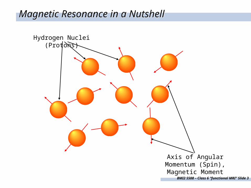
Magnetic Resonance in a NutshellMagnetic Resonance in a Nutshell
Hydrogen Nuclei (Protons)
Axis of Angular Momentum (Spin), Magnetic Moment
BMI2 SS08 – Class 6 “functional MRI” Slide 4
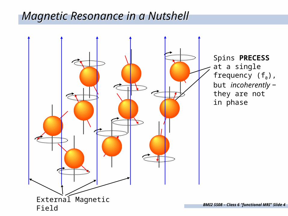
Magnetic Resonance in a NutshellMagnetic Resonance in a Nutshell
Spins PRECESS at a single frequency (f0), but incoherently − they are not in phase
External Magnetic Field
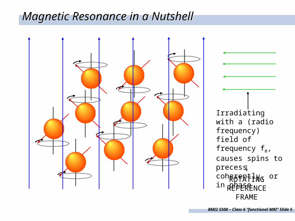
BMI2 SS08 – Class 6 “functional MRI” Slide 5
Magnetic Resonance in a NutshellMagnetic Resonance in a Nutshell
Irradiating with a (radio frequency) field of frequency f0, causes spins to precess coherently, or in phase
↓ROTATING
REFERENCE FRAME
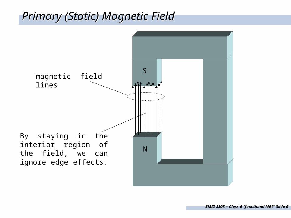
BMI2 SS08 – Class 6 “functional MRI” Slide 6
Primary (Static) Magnetic FieldPrimary (Static) Magnetic Field
N
Smagnetic field lines
By staying in the interior region of the field, we can ignore edge effects.
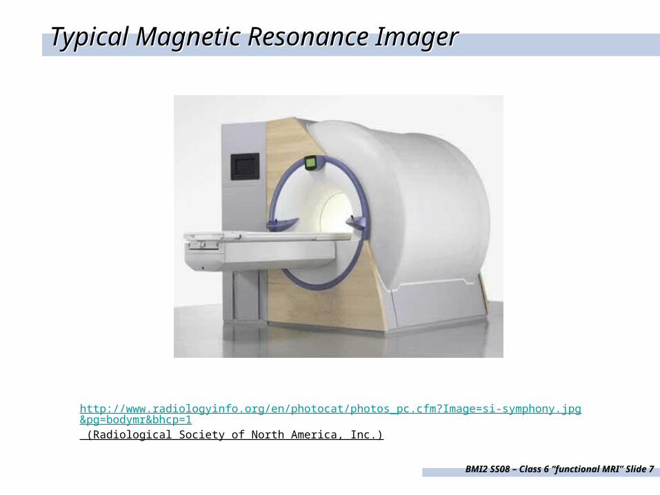
BMI2 SS08 – Class 6 “functional MRI” Slide 7
Typical Magnetic Resonance ImagerTypical Magnetic Resonance Imager
http://www.radiologyinfo.org/en/photocat/photos_pc.cfm?Image=si-symphony.jpg&pg=bodymr&bhcp=1 (Radiological Society of North America, Inc.)
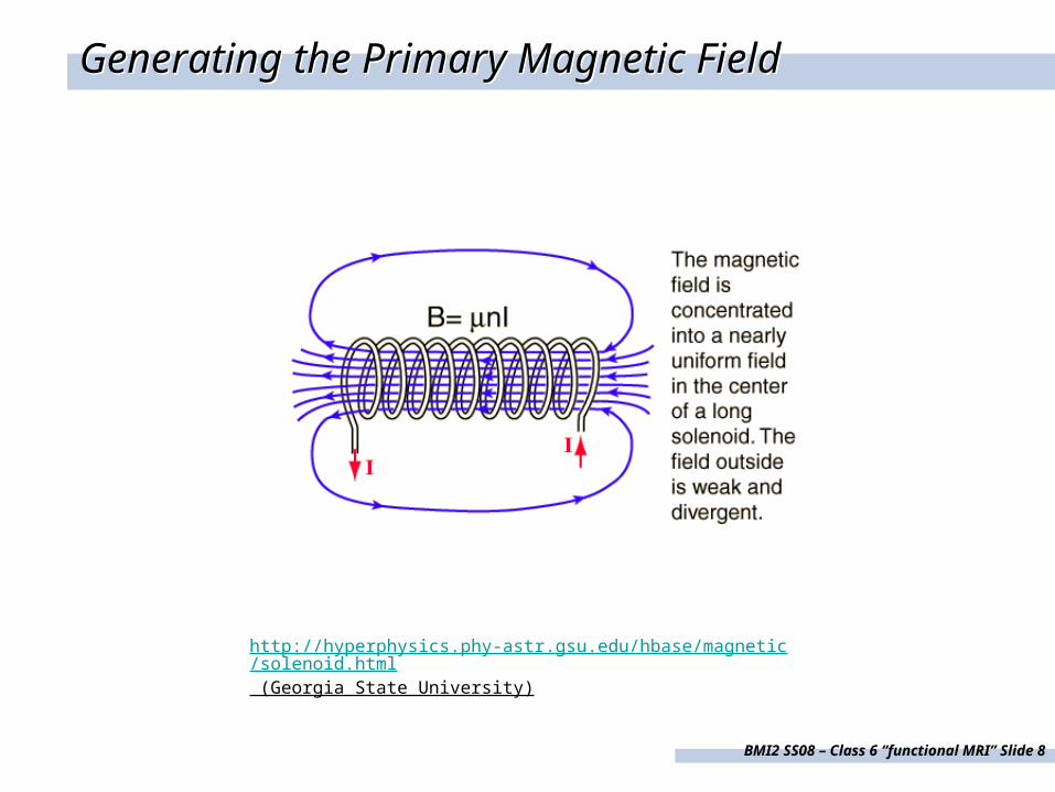
BMI2 SS08 – Class 6 “functional MRI” Slide 8
Generating the Primary Magnetic FieldGenerating the Primary Magnetic Field
http://hyperphysics.phy-astr.gsu.edu/hbase/magnetic/solenoid.html (Georgia State University)
BMI2 SS08 – Class 6 “functional MRI” Slide 9
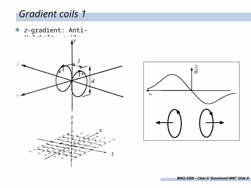
Gradient coils 1Gradient coils 1
z-gradient: Anti-Helmholtz coils
BMI2 SS08 – Class 6 “functional MRI” Slide 10
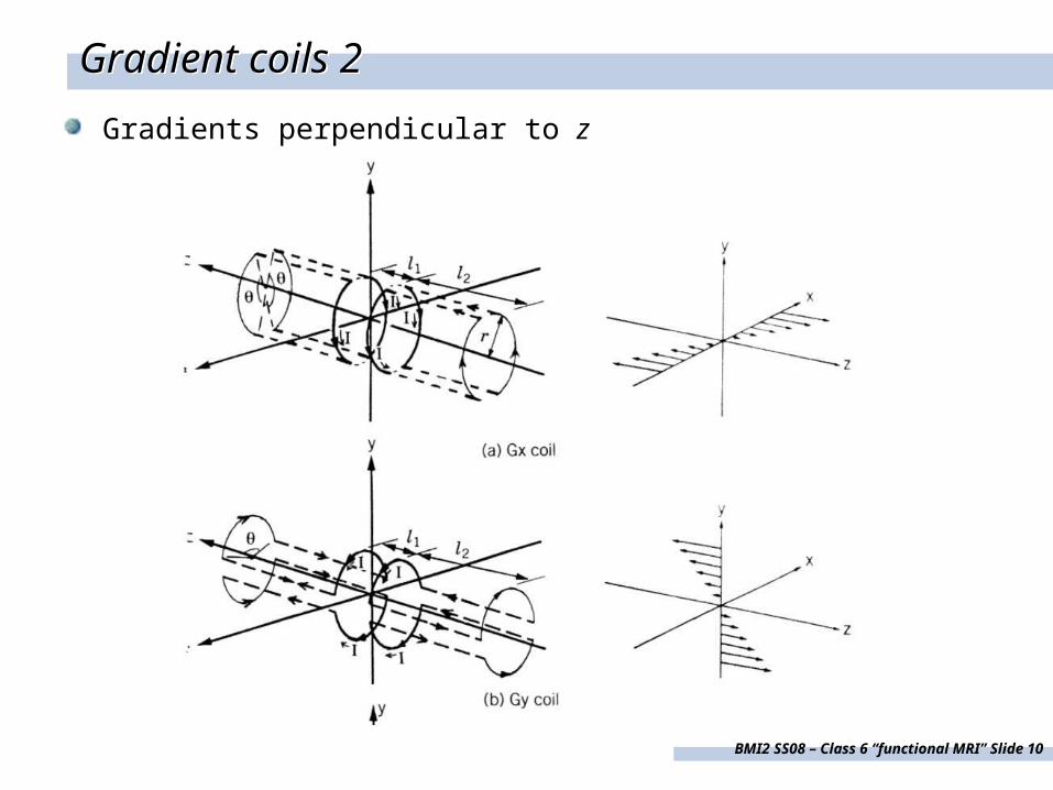
Gradient coils 2Gradient coils 2
Gradients perpendicular to z
BMI2 SS08 – Class 6 “functional MRI” Slide 11
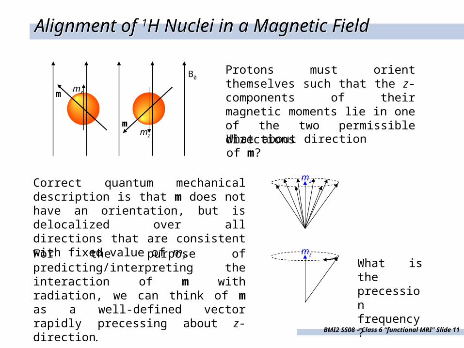
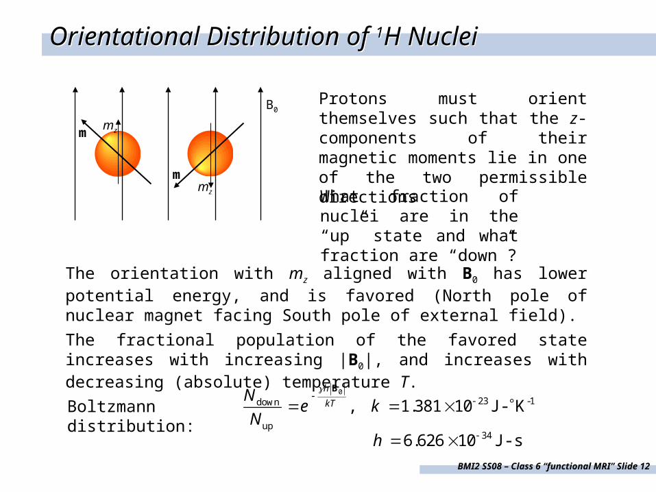
Alignment of 1H Nuclei in a Magnetic FieldAlignment of 1H Nuclei in a Magnetic Field
mmz
mmz
B0Protons must orient themselves such that the z-components of their magnetic moments lie in one of the two permissible directions
What about direction of m?
mzCorrect quantum mechanical description is that m does not have an orientation, but is delocalized over all directions that are consistent with fixed value of mz.
For the purpose of predicting/interpreting the interaction of m with radiation, we can think of m as a well-defined vector rapidly precessing about z-direction.
mz
What is the precession frequency?
BMI2 SS08 – Class 6 “functional MRI” Slide 12
Orientational Distribution of 1H NucleiOrientational Distribution of 1H Nuclei
What fraction of nuclei are in the “up” state and what fraction are “down”?
mmz
mmz
B0Protons must orient themselves such that the z-components of their magnetic moments lie in one of the two permissible directions
The orientation with mz aligned with B0 has lower potential energy, and is favored (North pole of nuclear magnet facing South pole of external field).
The fractional population of the favored state increases with increasing |B0|, and increases with decreasing (absolute) temperature T.
Boltzmann distribution: 0
23 -1down
up34
, 1.381 10 J - K
6.626 10 J - s
h
kTN
e kN
h
B
BMI2 SS08 – Class 6 “functional MRI” Slide 13
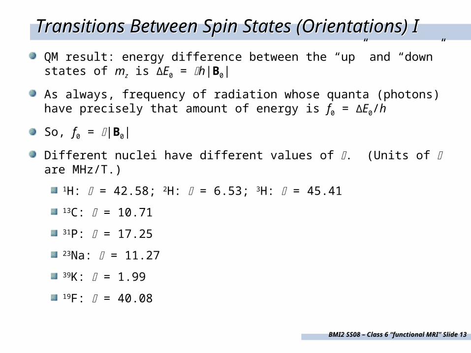
Transitions Between Spin States (Orientations) ITransitions Between Spin States (Orientations) I
QM result: energy difference between the “up” and “down” states of mz is ΔE0 = h|B0|
As always, frequency of radiation whose quanta (photons) have precisely that amount of energy is f0 = ΔE0/h
So, f0 = |B0|
Different nuclei have different values of . (Units of are MHz/T.)
1H: = 42.58; 2H: = 6.53; 3H: = 45.41
13C: = 10.71
31P: = 17.25
23Na: = 11.27
39K: = 1.99
19F: = 40.08
BMI2 SS08 – Class 6 “functional MRI” Slide 14
Transitions Between Spin States IITransitions Between Spin States II
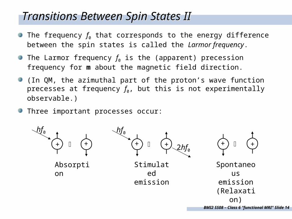
The frequency f0 that corresponds to the energy difference between the spin states is called the Larmor frequency.
The Larmor frequency f0 is the (apparent) precession frequency for m about the magnetic field direction.
(In QM, the azimuthal part of the proton’s wave function precesses at frequency f0, but this is not experimentally observable.)
Three important processes occur:
+
+
+
+
+
+
hf0 hf0
2hf0
Absorption Stimulated emission
Spontaneous emission
(Relaxation)
BMI2 SS08 – Class 6 “functional MRI” Slide 15
Transitions Between Spin States IIITransitions Between Spin States III
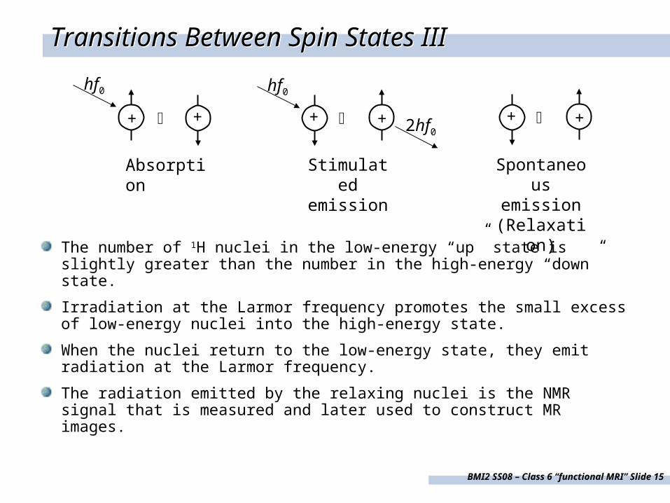
The number of 1H nuclei in the low-energy “up” state is slightly greater than the number in the high-energy “down” state.
Irradiation at the Larmor frequency promotes the small excess of low-energy nuclei into the high-energy state.
When the nuclei return to the low-energy state, they emit radiation at the Larmor frequency.
The radiation emitted by the relaxing nuclei is the NMR signal that is measured and later used to construct MR images.
+
+
+
+
+
+
hf0 hf0
2hf0
Absorption Stimulated emission
Spontaneous emission
(Relaxation)
BMI2 SS08 – Class 6 “functional MRI” Slide 16
SaturationSaturation
Suppose the average time required for an excited nucleus to return to the ground state is long (low relaxation rate, long excited-state lifetime)
If the external radiation is intense or is kept on for a long time, ground-state nuclei may be promoted to the excited state faster than they can return to the ground state.
Eventually, an exact 50/50 distribution of nuclei in the ground and excited states is reached
At this point the system is saturated. No NMR signal is produced, because the rates of “up”→“down” and “down”→“up” transitions are equal.
BMI2 SS08 – Class 6 “functional MRI” Slide 17
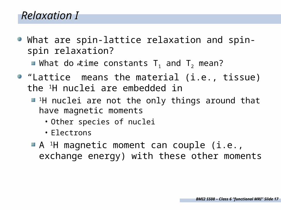
Relaxation IRelaxation I
What are spin-lattice relaxation and spin-spin relaxation?What do time constants T1 and T2 mean?
“Lattice” means the material (i.e., tissue) the 1H nuclei are embedded in
1H nuclei are not the only things around that have magnetic moments
• Other species of nuclei• Electrons
A 1H magnetic moment can couple (i.e., exchange energy) with these other moments
BMI2 SS08 – Class 6 “functional MRI” Slide 18
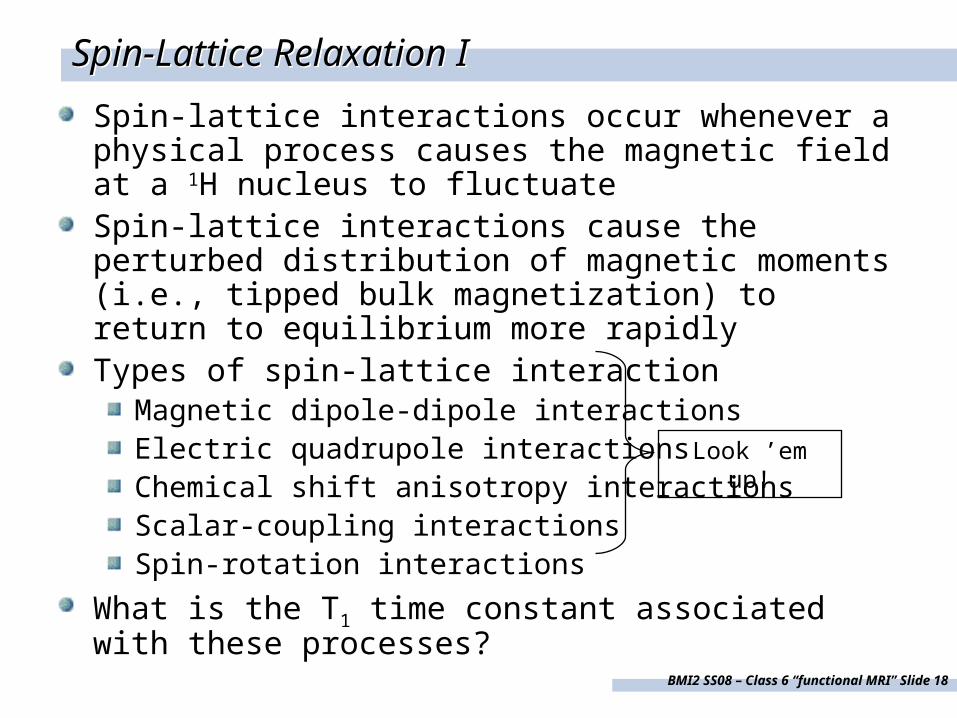
Spin-Lattice Relaxation ISpin-Lattice Relaxation I
Spin-lattice interactions occur whenever a physical process causes the magnetic field at a 1H nucleus to fluctuateSpin-lattice interactions cause the perturbed distribution of magnetic moments (i.e., tipped bulk magnetization) to return to equilibrium more rapidlyTypes of spin-lattice interaction
Magnetic dipole-dipole interactionsElectric quadrupole interactionsChemical shift anisotropy interactionsScalar-coupling interactionsSpin-rotation interactions
What is the T1 time constant associated with these processes?
Look ’em up!
BMI2 SS08 – Class 6 “functional MRI” Slide 19
x׳
y׳
z׳
B0
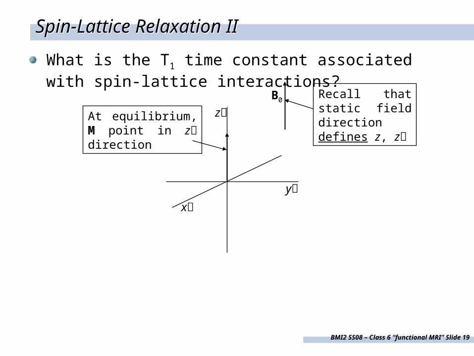
Spin-Lattice Relaxation IISpin-Lattice Relaxation II
What is the T1 time constant associated with spin-lattice interactions?
At equilibrium, M point in z׳ direction
Recall that static field direction defines z, z׳
BMI2 SS08 – Class 6 “functional MRI” Slide 20
x׳
y׳
z׳
B0
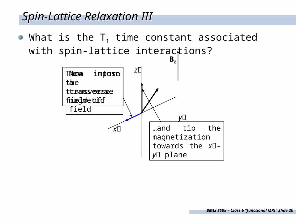
Spin-Lattice Relaxation IIISpin-Lattice Relaxation III
What is the T1 time constant associated with spin-lattice interactions?
Now impose a transverse magnetic field
…and tip the magnetization towards the x׳-y׳ plane
Then turn the transverse field off
BMI2 SS08 – Class 6 “functional MRI” Slide 21
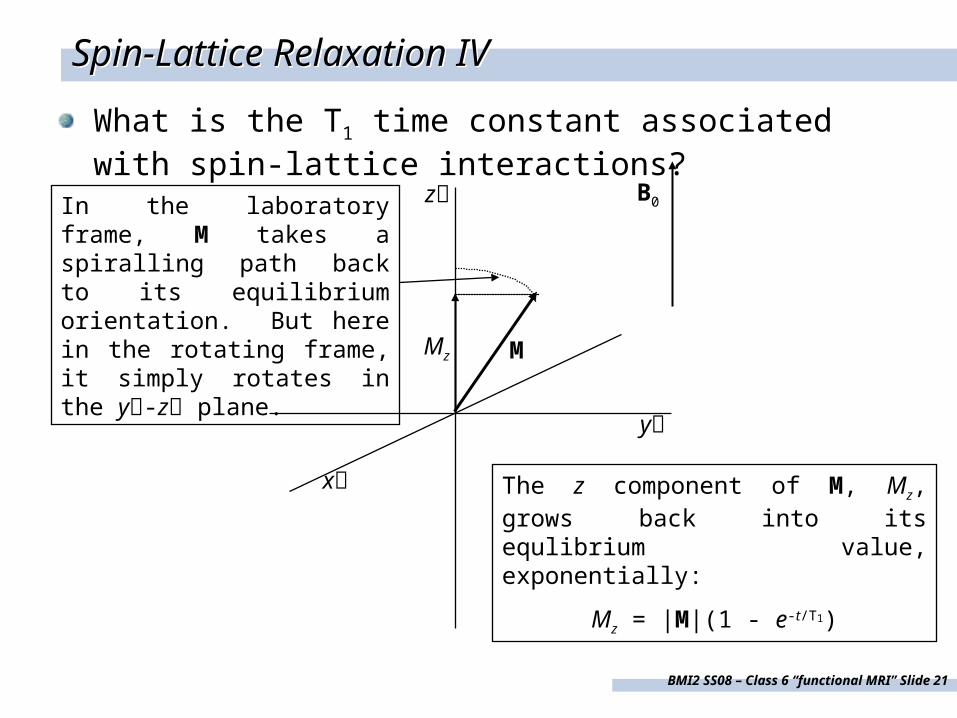
Spin-Lattice Relaxation IVSpin-Lattice Relaxation IV
What is the T1 time constant associated with spin-lattice interactions?
x׳
y׳
z׳ B0In the laboratory frame, M takes a spiralling path back to its equilibrium orientation. But here in the rotating frame, it simply rotates in the y׳-z׳ plane.
The z component of M, Mz, grows back into its equlibrium value, exponentially:
Mz = |M|(1 - e-t/T1)
Mz M
BMI2 SS08 – Class 6 “functional MRI” Slide 22
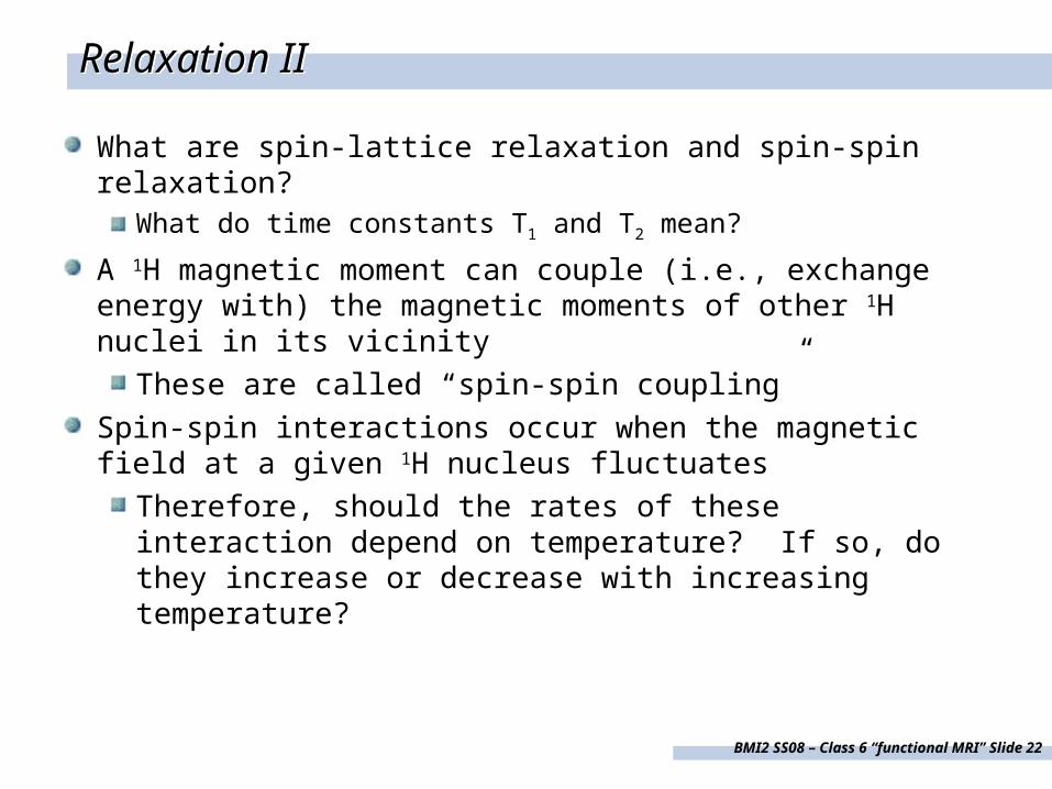
Relaxation IIRelaxation II
What are spin-lattice relaxation and spin-spin relaxation?What do time constants T1 and T2 mean?
A 1H magnetic moment can couple (i.e., exchange energy with) the magnetic moments of other 1H nuclei in its vicinity
These are called “spin-spin coupling”
Spin-spin interactions occur when the magnetic field at a given 1H nucleus fluctuates
Therefore, should the rates of these interaction depend on temperature? If so, do they increase or decrease with increasing temperature?
BMI2 SS08 – Class 6 “functional MRI” Slide 23
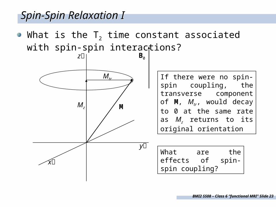
Spin-Spin Relaxation ISpin-Spin Relaxation I
What is the T2 time constant associated with spin-spin interactions?
x׳
y׳
z׳ B0
MMz
Mtr If there were no spin-spin coupling, the transverse component of M, Mtr, would decay to 0 at the same rate as Mz returns to its original orientation
What are the effects of spin-spin coupling?
BMI2 SS08 – Class 6 “functional MRI” Slide 24
Spin-Spin Relaxation IISpin-Spin Relaxation II
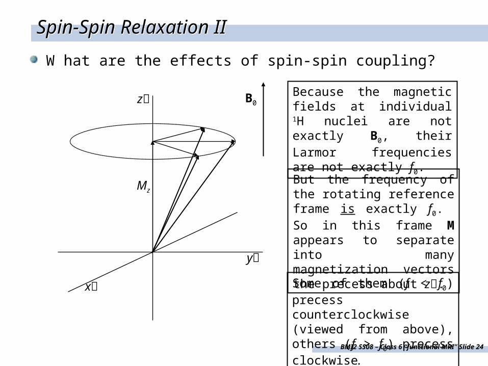
W hat are the effects of spin-spin coupling?
Because the magnetic fields at individual 1H nuclei are not exactly B0, their Larmor frequencies are not exactly f0.
x׳
y׳
z׳ B0
MzBut the frequency of the rotating reference frame is exactly f0. So in this frame M appears to separate into many magnetization vectors the precess about z׳.
Some of them (f < f0) precess counterclockwise (viewed from above), others (f > f0) precess clockwise.
BMI2 SS08 – Class 6 “functional MRI” Slide 25
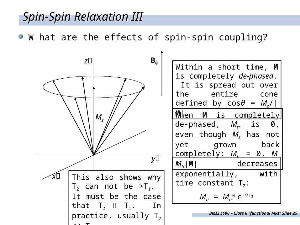
Spin-Spin Relaxation IIISpin-Spin Relaxation III
W hat are the effects of spin-spin coupling?
Within a short time, M is completely de-phased. It is spread out over the entire cone defined by cosθ = Mz/|M|
x׳
y׳
z׳ B0
MzWhen M is completely de-phased, Mtr is 0, even though Mz has not yet grown back completely: Mtr = 0, Mz < |M|
Mtr decreases exponentially, with time constant T2:
Mtr = Mtr0 e-t/T2
This also shows why T2 can not be >T1. It must be the case that T2 T1. In practice, usually T2 << T1.
BMI2 SS08 – Class 6 “functional MRI” Slide 26
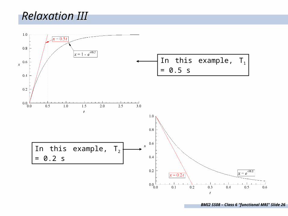
Relaxation IIIRelaxation III
In this example, T1 = 0.5 s
In this example, T2 = 0.2 s
BMI2 SS08 – Class 6 “functional MRI” Slide 27
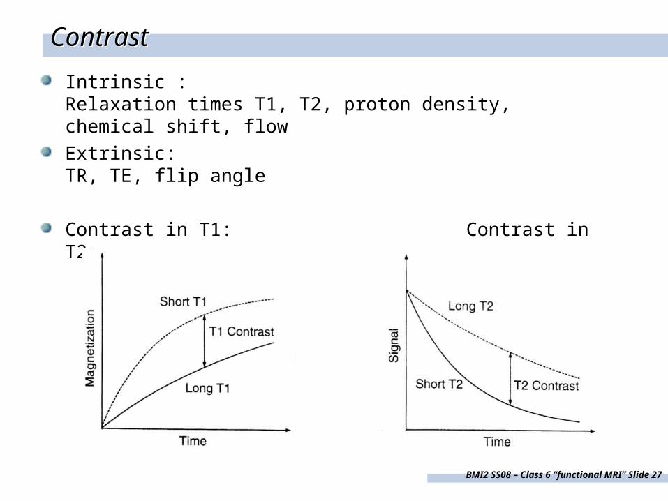
ContrastContrast
Intrinsic : Relaxation times T1, T2, proton density, chemical shift, flow
Extrinsic: TR, TE, flip angle
Contrast in T1: Contrast in T2:
BMI2 SS08 – Class 6 “functional MRI” Slide 28
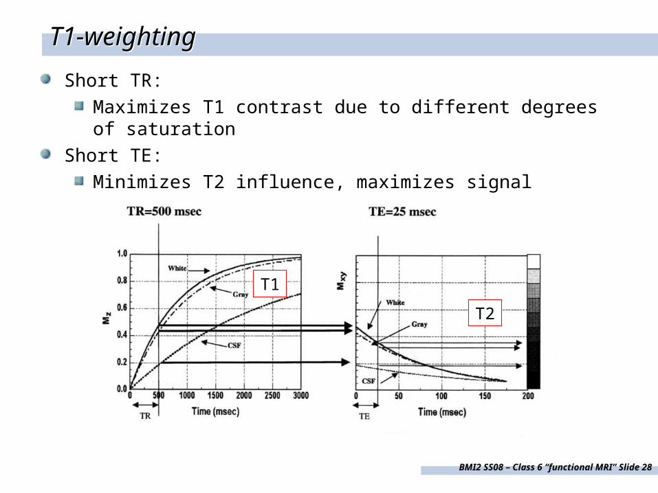
T1-weightingT1-weighting
Short TR:
Maximizes T1 contrast due to different degrees of saturation
Short TE:
Minimizes T2 influence, maximizes signal
T1
T2
BMI2 SS08 – Class 6 “functional MRI” Slide 29
T1
T2
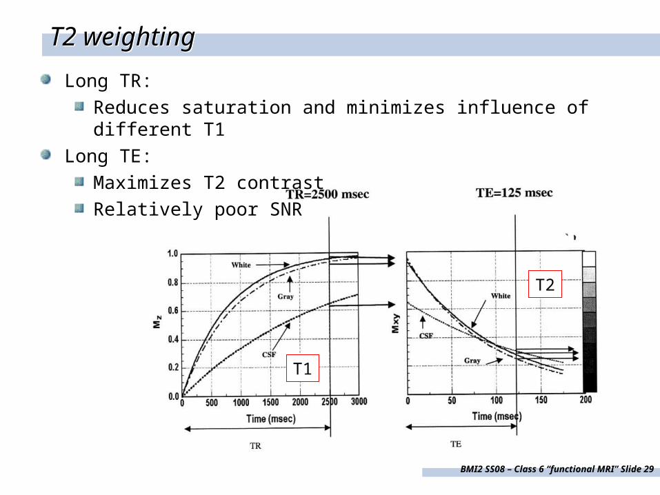
T2 weightingT2 weighting
Long TR:
Reduces saturation and minimizes influence of different T1
Long TE:
Maximizes T2 contrast
Relatively poor SNR
BMI2 SS08 – Class 6 “functional MRI” Slide 30
T1
T2
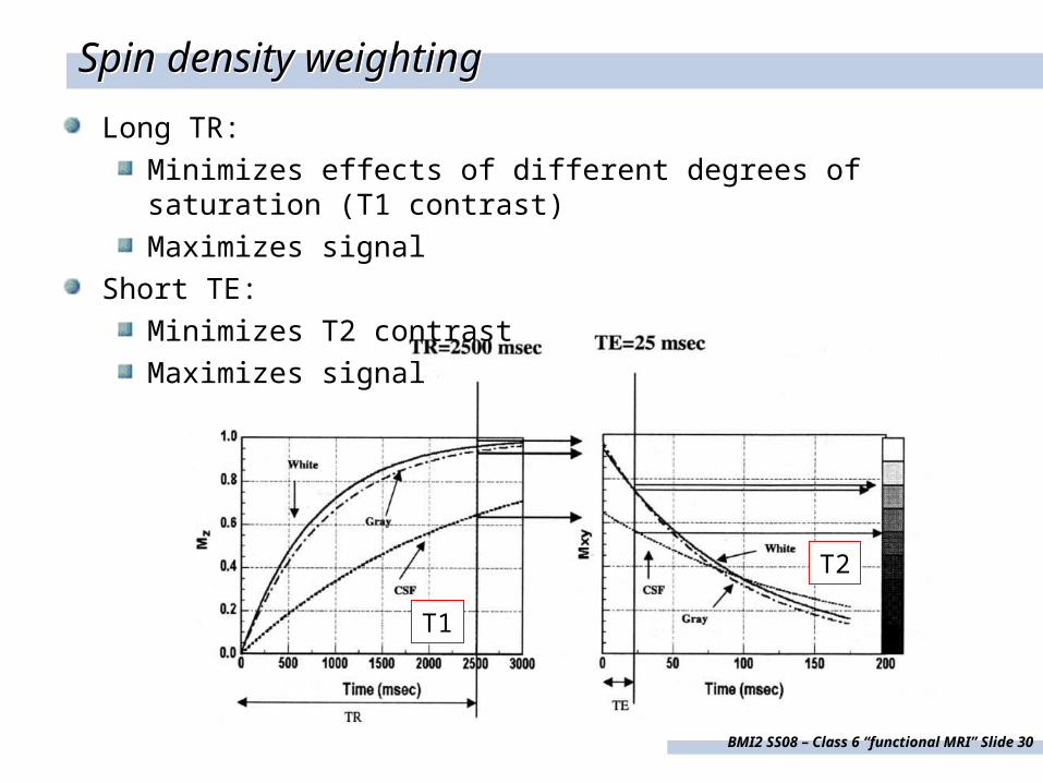
Spin density weightingSpin density weighting
Long TR:
Minimizes effects of different degrees of saturation (T1 contrast)
Maximizes signal
Short TE:
Minimizes T2 contrast
Maximizes signal
BMI2 SS08 – Class 6 “functional MRI” Slide 31
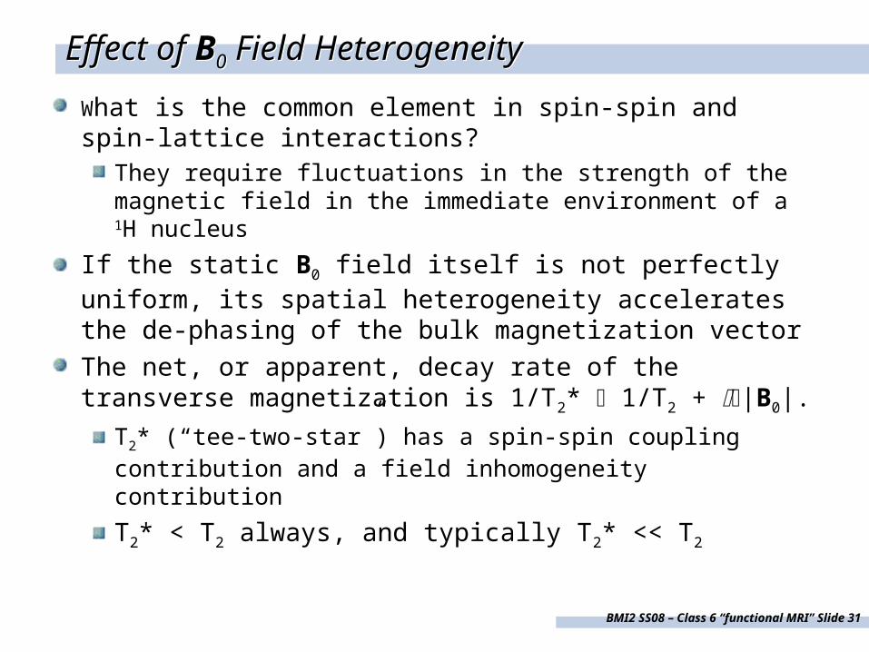
Effect of B0 Field HeterogeneityEffect of B0 Field Heterogeneity
What is the common element in spin-spin and spin-lattice interactions?
They require fluctuations in the strength of the magnetic field in the immediate environment of a 1H nucleus
If the static B0 field itself is not perfectly uniform, its spatial heterogeneity accelerates the de-phasing of the bulk magnetization vector
The net, or apparent, decay rate of the transverse magnetization is 1/T2* 1/T2 + |B0|.
T2* (“tee-two-star”) has a spin-spin coupling contribution and a field inhomogeneity contribution
T2* < T2 always, and typically T2* << T2
BMI2 SS08 – Class 6 “functional MRI” Slide 32
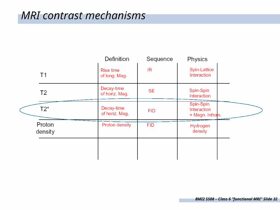
MRI contrast mechanismsMRI contrast mechanisms
BMI2 SS08 – Class 6 “functional MRI” Slide 33
MR Imaging PrinciplesMR Imaging Principles
BMI2 SS08 – Class 6 “functional MRI” Slide 34
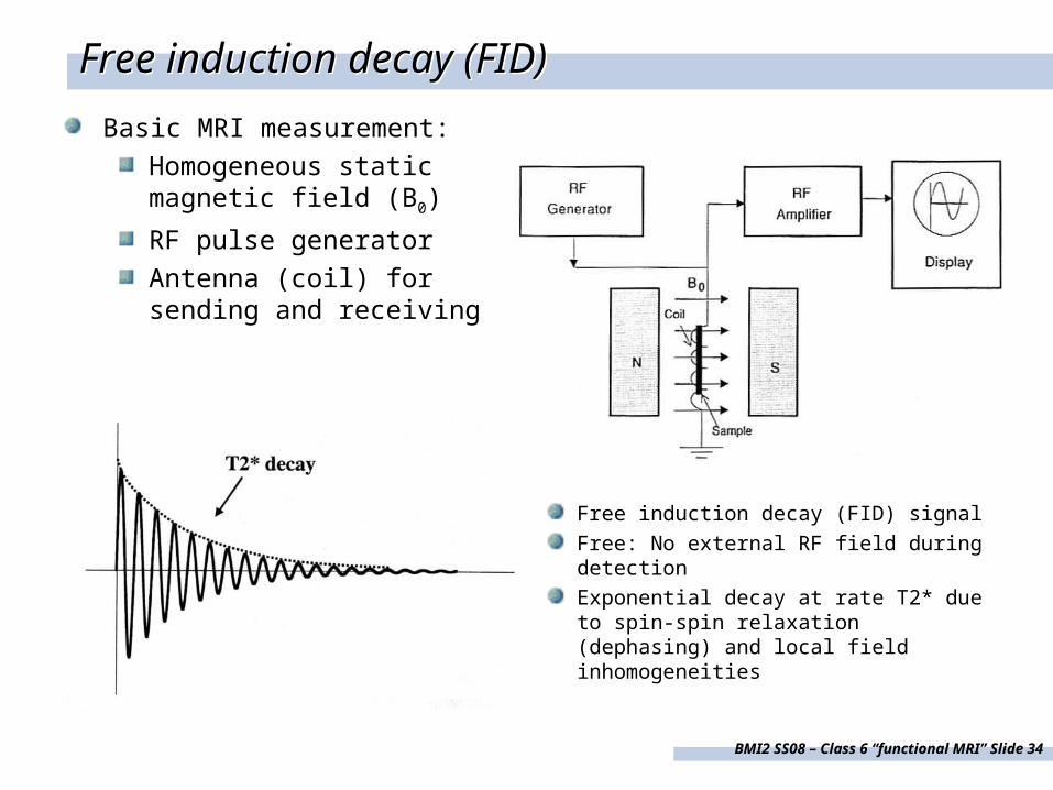
Free induction decay (FID)Free induction decay (FID)
Basic MRI measurement:
Homogeneous static magnetic field (B0)
RF pulse generator
Antenna (coil) for sending and receiving
Free induction decay (FID) signal
Free: No external RF field during detection
Exponential decay at rate T2* due to spin-spin relaxation (dephasing) and local field inhomogeneities
BMI2 SS08 – Class 6 “functional MRI” Slide 35
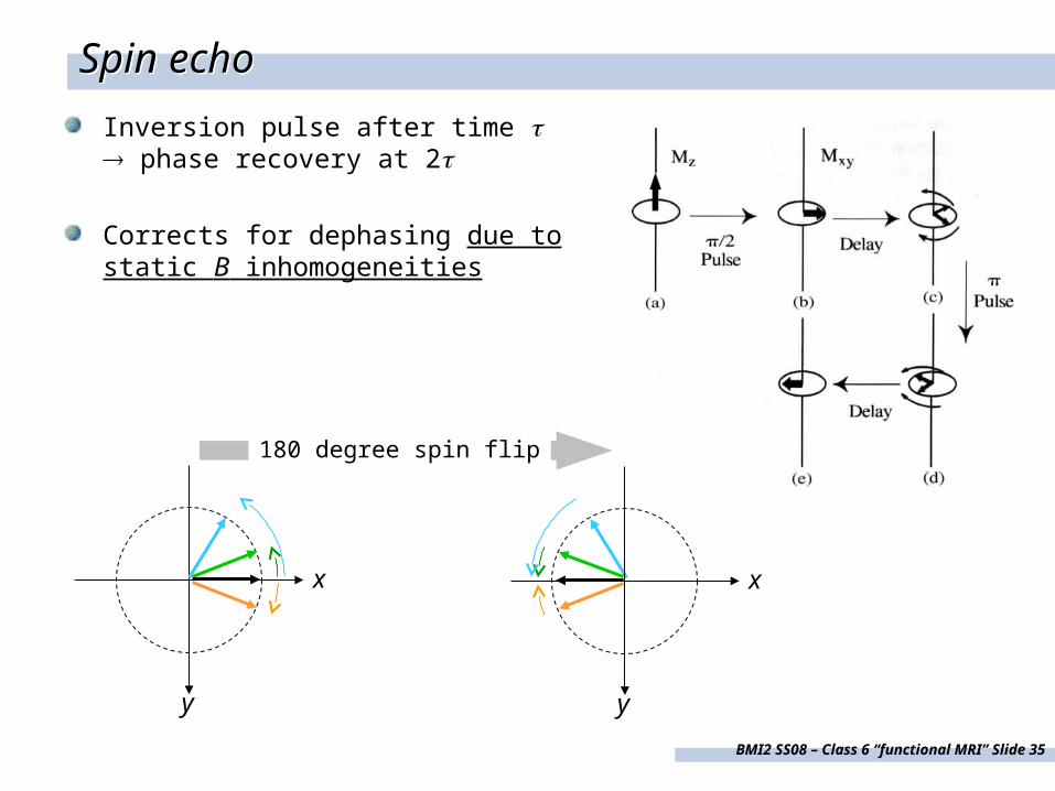
Spin echoSpin echo
Inversion pulse after time phase recovery at 2
Corrects for dephasing due to static B inhomogeneities
x
y
x
y
180 degree spin flip
BMI2 SS08 – Class 6 “functional MRI” Slide 36
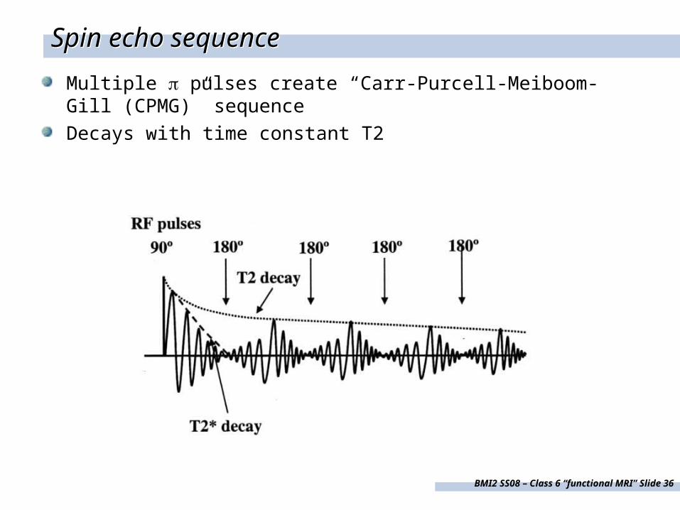
Spin echo sequenceSpin echo sequence
Multiple pulses create “Carr-Purcell-Meiboom-Gill (CPMG)” sequence
Decays with time constant T2
BMI2 SS08 – Class 6 “functional MRI” Slide 37
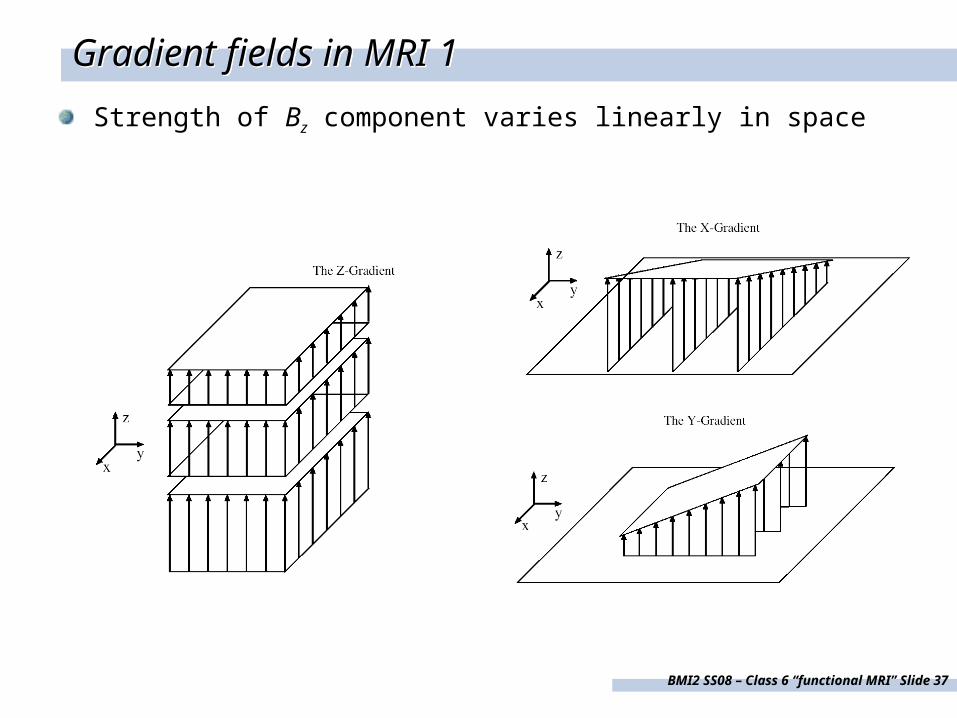
Gradient fields in MRI 1Gradient fields in MRI 1
Strength of Bz component varies linearly in space
BMI2 SS08 – Class 6 “functional MRI” Slide 38
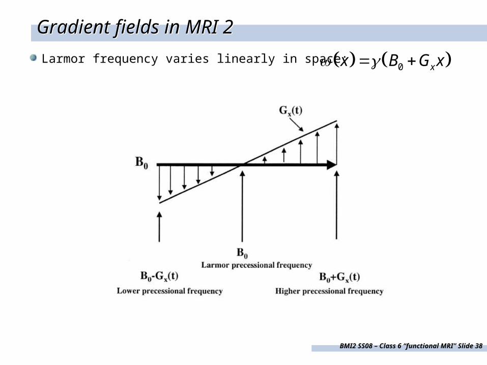
Gradient fields in MRI 2Gradient fields in MRI 2
Larmor frequency varies linearly in space: 0 xx B G x
BMI2 SS08 – Class 6 “functional MRI” Slide 39
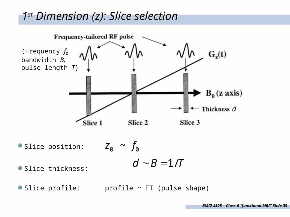
1st Dimension (z): Slice selection1st Dimension (z): Slice selection
Slice position: z0 ~ f0
Slice thickness:
Slice profile: profile ~ FT (pulse shape)
1/d B T
d
(Frequency f0
bandwidth B, pulse length T)
BMI2 SS08 – Class 6 “functional MRI” Slide 40
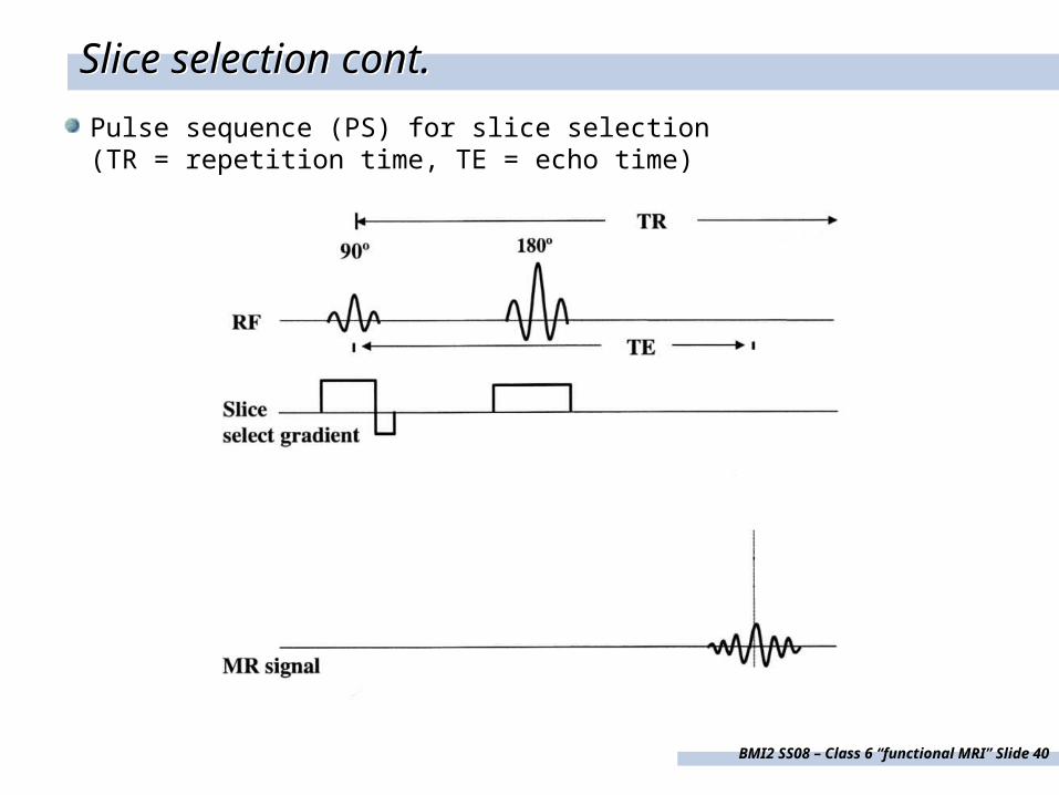
Slice selection cont.Slice selection cont.
Pulse sequence (PS) for slice selection (TR = repetition time, TE = echo time)
BMI2 SS08 – Class 6 “functional MRI” Slide 41
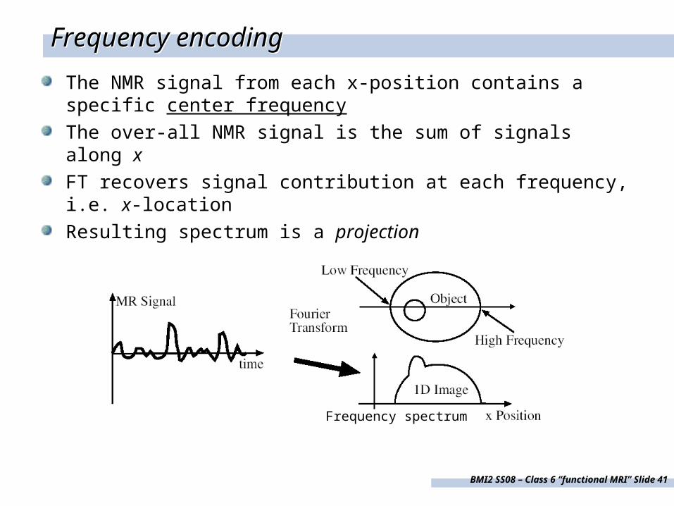
Frequency encodingFrequency encoding
The NMR signal from each x-position contains a specific center frequency
The over-all NMR signal is the sum of signals along x
FT recovers signal contribution at each frequency, i.e. x-location
Resulting spectrum is a projection
Frequency spectrum
BMI2 SS08 – Class 6 “functional MRI” Slide 42
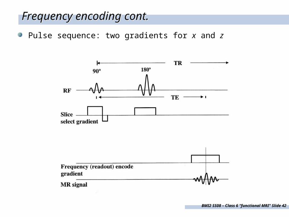
Frequency encoding cont.Frequency encoding cont.
Pulse sequence: two gradients for x and z
BMI2 SS08 – Class 6 “functional MRI” Slide 43
3rd Dimension (y)3rd Dimension (y)
How to achieve y-localization? Frequency encoding will always produce iso-lines of resonance frequencies
Solution:
Reconstruction from projections
Phase encoding
BMI2 SS08 – Class 6 “functional MRI” Slide 44
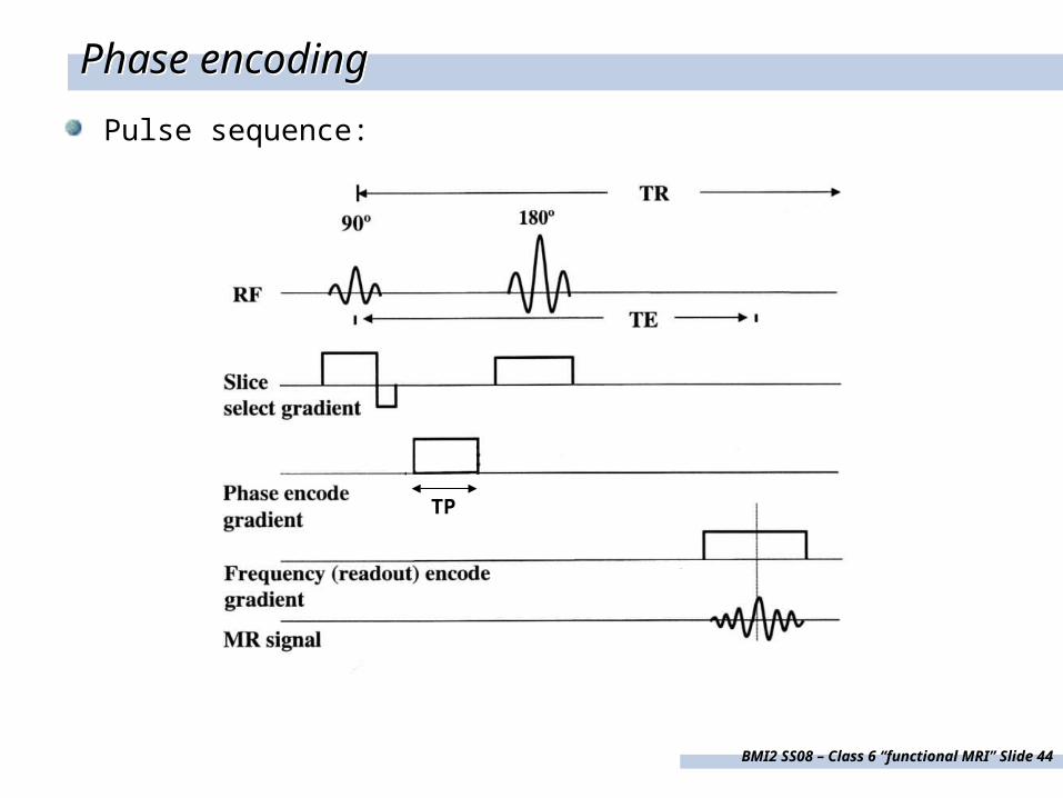
Phase encodingPhase encoding
Pulse sequence:
TP
BMI2 SS08 – Class 6 “functional MRI” Slide 45
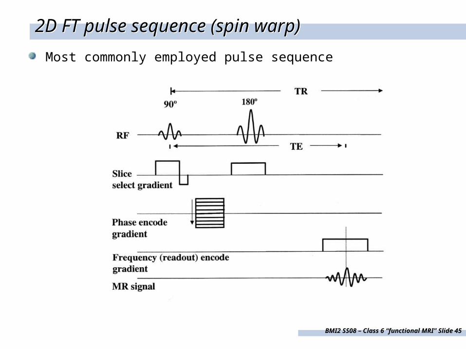
2D FT pulse sequence (spin warp)2D FT pulse sequence (spin warp)
Most commonly employed pulse sequence
BMI2 SS08 – Class 6 “functional MRI” Slide 46
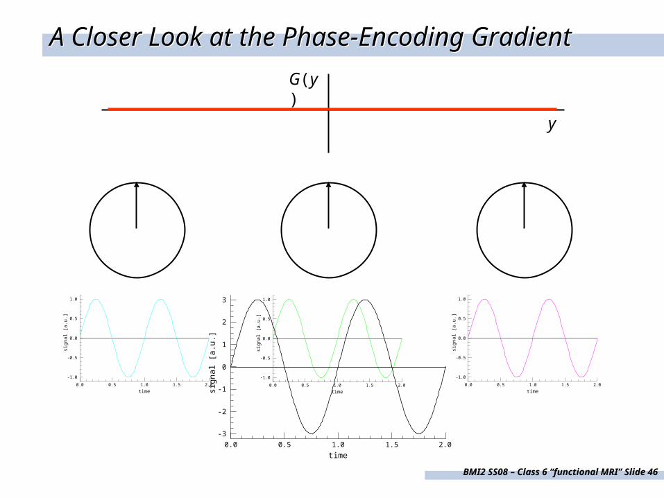
A Closer Look at the Phase-Encoding GradientA Closer Look at the Phase-Encoding Gradient
y
G(y)
time
0.0 0.5 1.0 1.5 2.0
sign
al [
a.u.
]
-1.0
-0.5
0.0
0.5
1.0
time
0.0 0.5 1.0 1.5 2.0
sign
al [
a.u.
]
-1.0
-0.5
0.0
0.5
1.0
time
0.0 0.5 1.0 1.5 2.0
sign
al [
a.u.
]
-1.0
-0.5
0.0
0.5
1.0
time
0.0 0.5 1.0 1.5 2.0
sign
al [
a.u.
]
-3
-2
-1
0
1
2
3
BMI2 SS08 – Class 6 “functional MRI” Slide 47
time
0.0 0.5 1.0 1.5 2.0
sign
al [
a.u.
]
-3
-2
-1
0
1
2
3
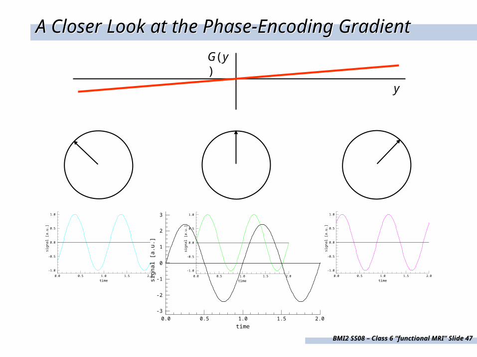
A Closer Look at the Phase-Encoding GradientA Closer Look at the Phase-Encoding Gradient
y
G(y)
time
0.0 0.5 1.0 1.5 2.0
sign
al [
a.u.
]
-1.0
-0.5
0.0
0.5
1.0
time
0.0 0.5 1.0 1.5 2.0
sign
al [
a.u.
]
-1.0
-0.5
0.0
0.5
1.0
time
0.0 0.5 1.0 1.5 2.0
sign
al [
a.u.
]
-1.0
-0.5
0.0
0.5
1.0
BMI2 SS08 – Class 6 “functional MRI” Slide 48
time
0.0 0.5 1.0 1.5 2.0
sign
al [
a.u.
]
-3
-2
-1
0
1
2
3
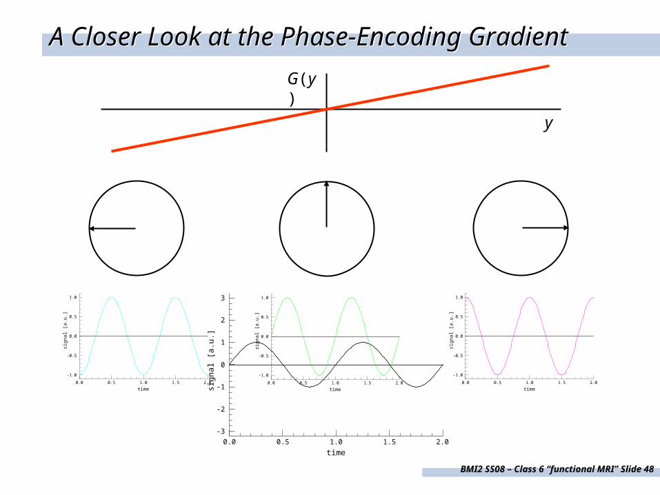
A Closer Look at the Phase-Encoding GradientA Closer Look at the Phase-Encoding Gradient
y
G(y)
time
0.0 0.5 1.0 1.5 2.0
sign
al [
a.u.
]
-1.0
-0.5
0.0
0.5
1.0
time
0.0 0.5 1.0 1.5 2.0
sign
al [
a.u.
]
-1.0
-0.5
0.0
0.5
1.0
time
0.0 0.5 1.0 1.5 2.0
sign
al [
a.u.
]
-1.0
-0.5
0.0
0.5
1.0
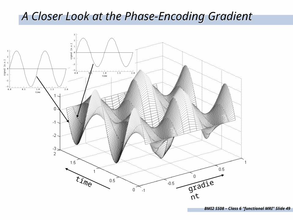
BMI2 SS08 – Class 6 “functional MRI” Slide 49
A Closer Look at the Phase-Encoding GradientA Closer Look at the Phase-Encoding Gradient
timegradient
time
0.0 0.5 1.0 1.5 2.0si
gnal
[a.
u.]
-3
-2
-1
0
1
2
3
time
0.0 0.5 1.0 1.5 2.0
sign
al [
a.u.
]
-3
-2
-1
0
1
2
3
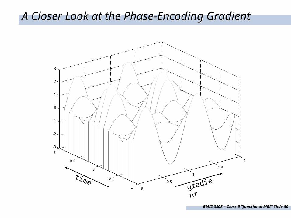
BMI2 SS08 – Class 6 “functional MRI” Slide 50
0
0.5
1
1.5
2
-1
-0.5
0
0.5
1-3
-2
-1
0
1
2
3
A Closer Look at the Phase-Encoding GradientA Closer Look at the Phase-Encoding Gradient
timegradient
BMI2 SS08 – Class 6 “functional MRI” Slide 51
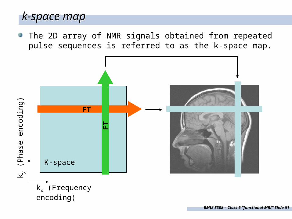
k-space mapk-space map
The 2D array of NMR signals obtained from repeated pulse sequences is referred to as the k-space map.
kx (Frequency encoding)
FT
k y (
Pha
se e
ncod
ing)
FT
K-space
BMI2 SS08 – Class 6 “functional MRI” Slide 52
From Structure to FunctionFrom Structure to Function
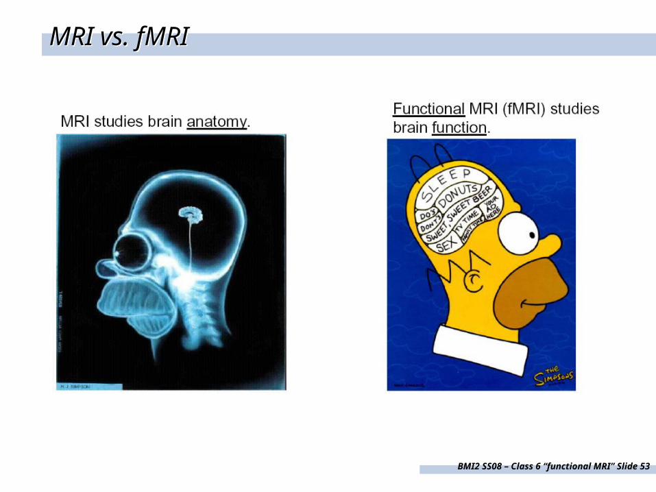
BMI2 SS08 – Class 6 “functional MRI” Slide 53
MRI vs. fMRIMRI vs. fMRI
BMI2 SS08 – Class 6 “functional MRI” Slide 54
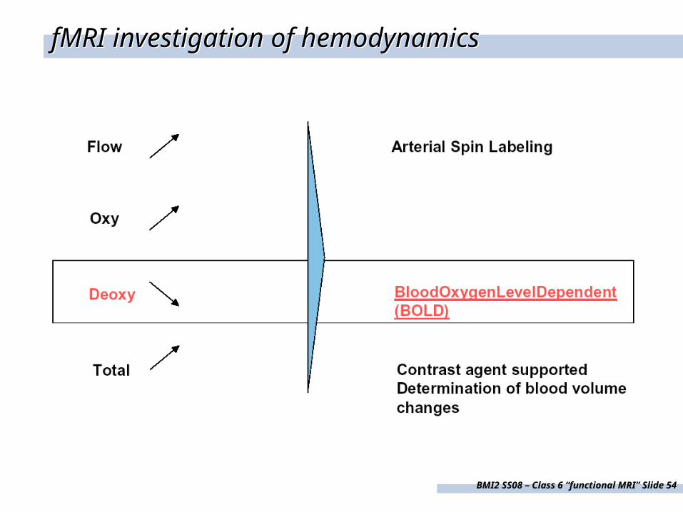
fMRI investigation of hemodynamicsfMRI investigation of hemodynamics
BMI2 SS08 – Class 6 “functional MRI” Slide 55
Magnetic Resonance Angiography (MRA)
Magnetic Resonance Angiography (MRA)
BMI2 SS08 – Class 6 “functional MRI” Slide 56
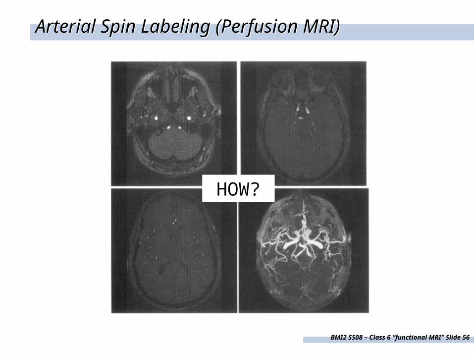
Arterial Spin Labeling (Perfusion MRI)Arterial Spin Labeling (Perfusion MRI)
HOW?
BMI2 SS08 – Class 6 “functional MRI” Slide 57
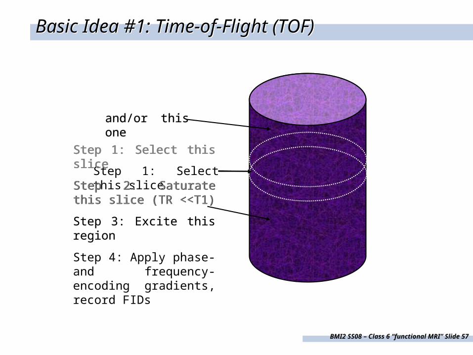
Basic Idea #1: Time-of-Flight (TOF)Basic Idea #1: Time-of-Flight (TOF)
Step 1: Select this slice
Step 2: Saturate this slice (TR <<T1)
Step 3: Excite this region
Step 4: Apply phase- and frequency-encoding gradients, record FIDs
and/or this one
Step 1: Select this slice
Step 1: Select this slice
Step 2: Saturate this slice (TR <<T1)
Step 1: Select this slice
Step 2: Saturate this slice (TR <<T1)
Step 3: Excite this region
and/or this one
BMI2 SS08 – Class 6 “functional MRI” Slide 58
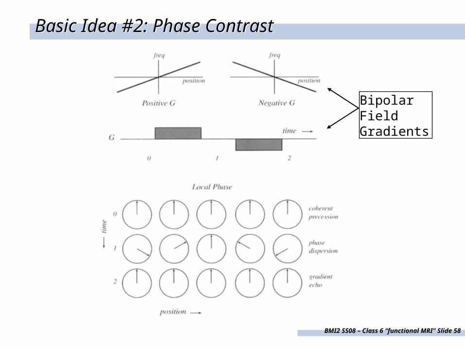
Basic Idea #2: Phase ContrastBasic Idea #2: Phase Contrast
Bipolar Field Gradients
BMI2 SS08 – Class 6 “functional MRI” Slide 59
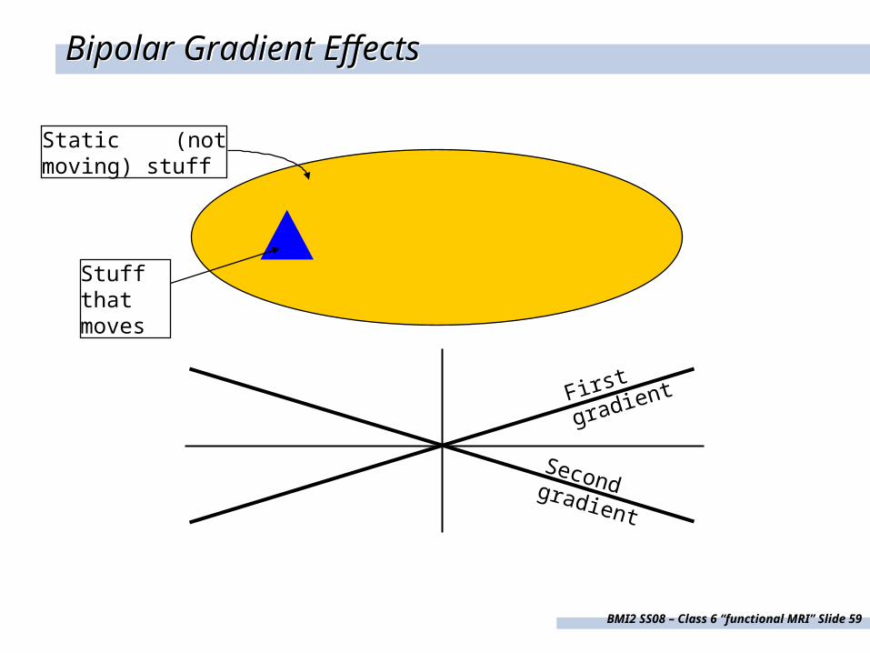
Bipolar Gradient EffectsBipolar Gradient Effects
Static (not moving) stuff
Stuff that moves
First gradient
Second gradient
BMI2 SS08 – Class 6 “functional MRI” Slide 60
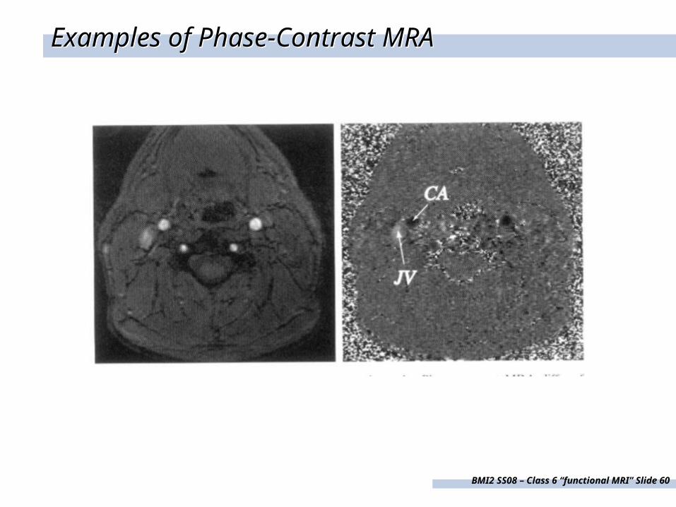
Examples of Phase-Contrast MRAExamples of Phase-Contrast MRA
BMI2 SS08 – Class 6 “functional MRI” Slide 61
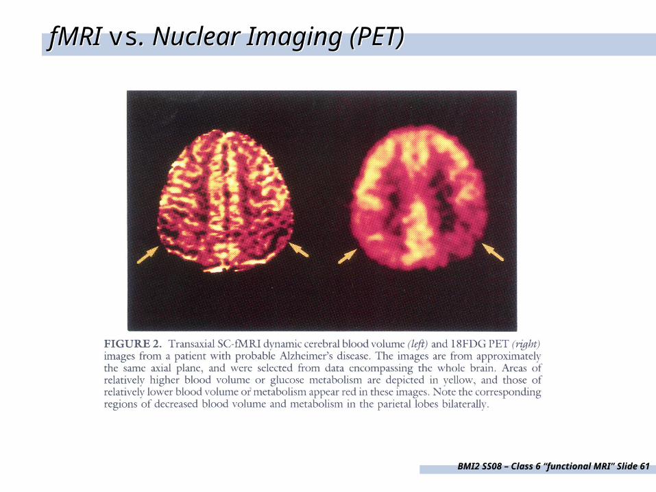
fMRI vs. Nuclear Imaging (PET)fMRI vs. Nuclear Imaging (PET)
BMI2 SS08 – Class 6 “functional MRI” Slide 62
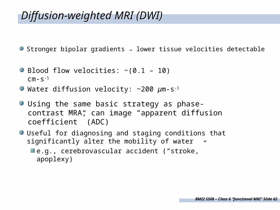
Diffusion-weighted MRI (DWI)Diffusion-weighted MRI (DWI)
Stronger bipolar gradients → lower tissue velocities detectable
Blood flow velocities: ~(0.1 – 10) cm-s-1
Water diffusion velocity: ~200 μm-s-1
Using the same basic strategy as phase-contrast MRA, can image “apparent diffusion coefficient” (ADC)
Useful for diagnosing and staging conditions that significantly alter the mobility of water
e.g., cerebrovascular accident (“stroke,” apoplexy)
BMI2 SS08 – Class 6 “functional MRI” Slide 63
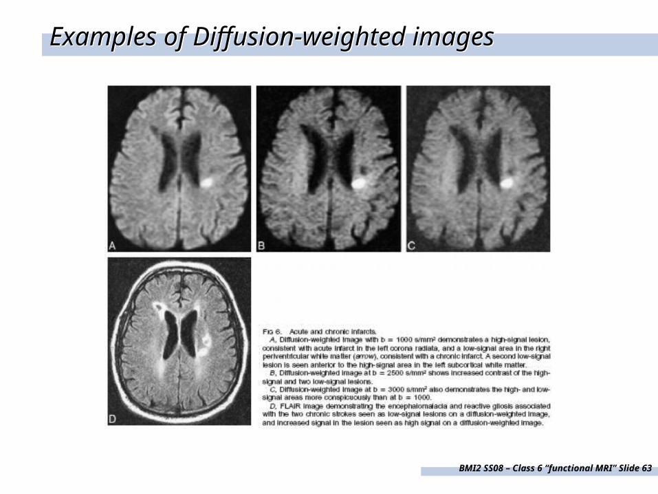
Examples of Diffusion-weighted imagesExamples of Diffusion-weighted images
BMI2 SS08 – Class 6 “functional MRI” Slide 64
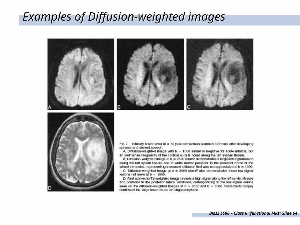
Examples of Diffusion-weighted imagesExamples of Diffusion-weighted images