bob plant - university of readingsws00rsp/teaching/nanjing/blayer.pdf · outline motivation some...

Boundary Layer ParameterizationBob Plant

With thanks to: R. Beare, S. Belcher, I. Boutle, O. Coceal, A. Grant, D. McNamara

NWP Physics Lecture 3

Nanjing Summer School

July 2014

Outline

Motivation

Some background on turbulence

Explicit turbulence simulations

Organization of the problem

Surface layer parameterization

K theory

The boundary layer grey zone

Boundary Layer parameterization – p.1/48

Motivation


Effects of the boundary layerControl simulation, T+60

950mb

Simulation with no boundary layer turbulence, T+60.

930mb

Simulations with (left) and without (right) boundary layer, ofstorm of 30/10/00


Role of friction: Ekman pumping

boundary layer top

surface

boundarylayer

free

tropopause

troposphere

ξ > ξ1 2

1

2ξ

ξ

Boundary layerconvergence leads toascent leads tospin-down of abarotropic vortex

Barotropic vorticityequation,

DζDt

= ζ∂w∂z

, ζ = f +ξ


Effects on low-level stability

Mid-level featureassociated with dryintrusion

Baroclinic frictionaleffects increaselow-level stability overthe low centre

Reduces the strengthof coupling betweentropopause-level PVfeature and surfacetemperature wave


Some background on turbulence


TKE

KE =12

u2 =12

(

u2 + v2 +w2)

+12

(

u′2 + v′2 +w′2)

+(uu′ + vv′ +ww′)

inc. KE of mean flow, KE of turbulence and cross terms

Reynolds average gives KE=mean flow KE + TKE

e =12

(

u′2 + v′2 +w′2)


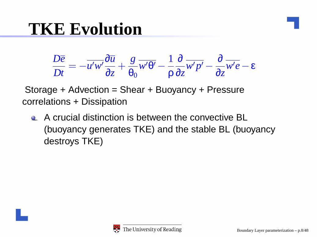
TKE Evolution

DeDt

= −u′w′∂u∂z

+gθ0

w′θ′−1ρ

∂∂z

w′p′−∂∂z

w′e− ε

Storage + Advection = Shear + Buoyancy + Pressurecorrelations + Dissipation

A crucial distinction is between the convective BL(buoyancy generates TKE) and the stable BL (buoyancydestroys TKE)


Typical TKE Budgets

Nocturnal, stable boundary layer Morning, well-mixedboundary layer


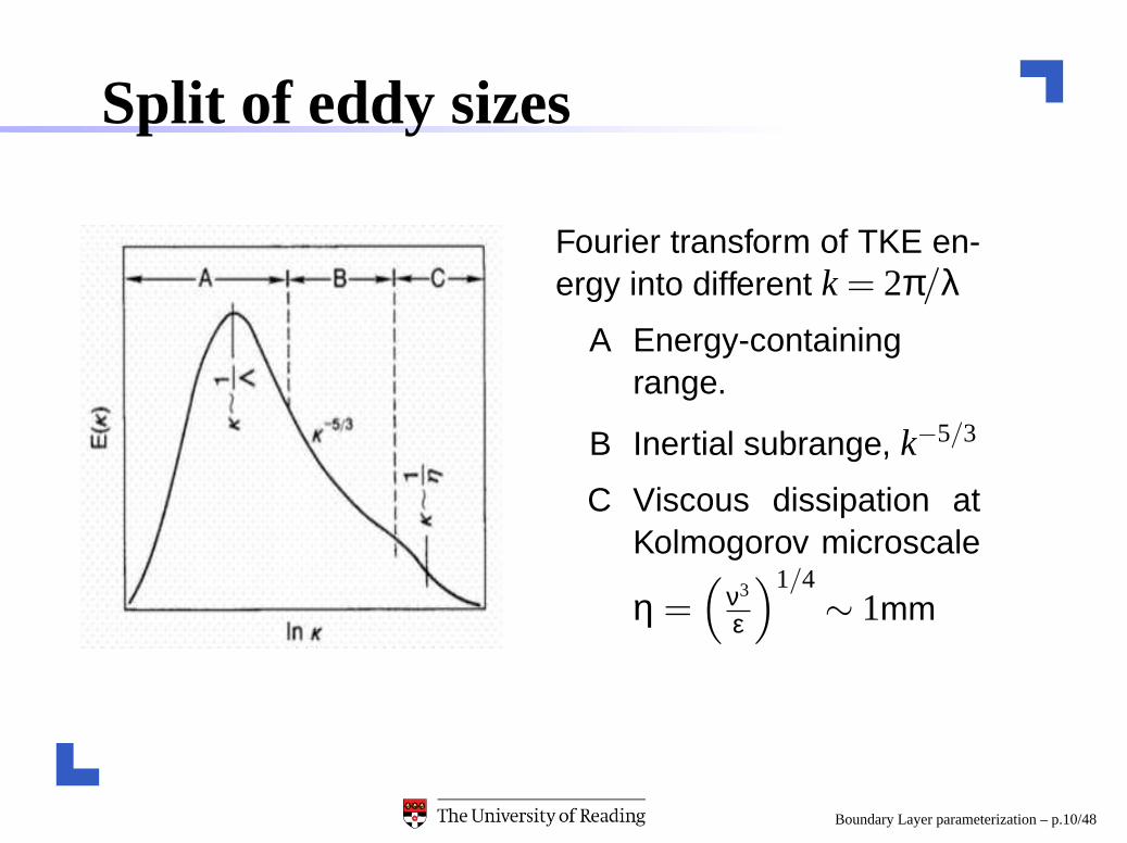
Split of eddy sizes

Fourier transform of TKE en-ergy into different k = 2π/λ

A Energy-containingrange.

B Inertial subrange, k−5/3

C Viscous dissipation atKolmogorov microscale

η =(

ν3

ε

)1/4∼ 1mm


Split of eddy sizes

The turbulent energy cas-cade


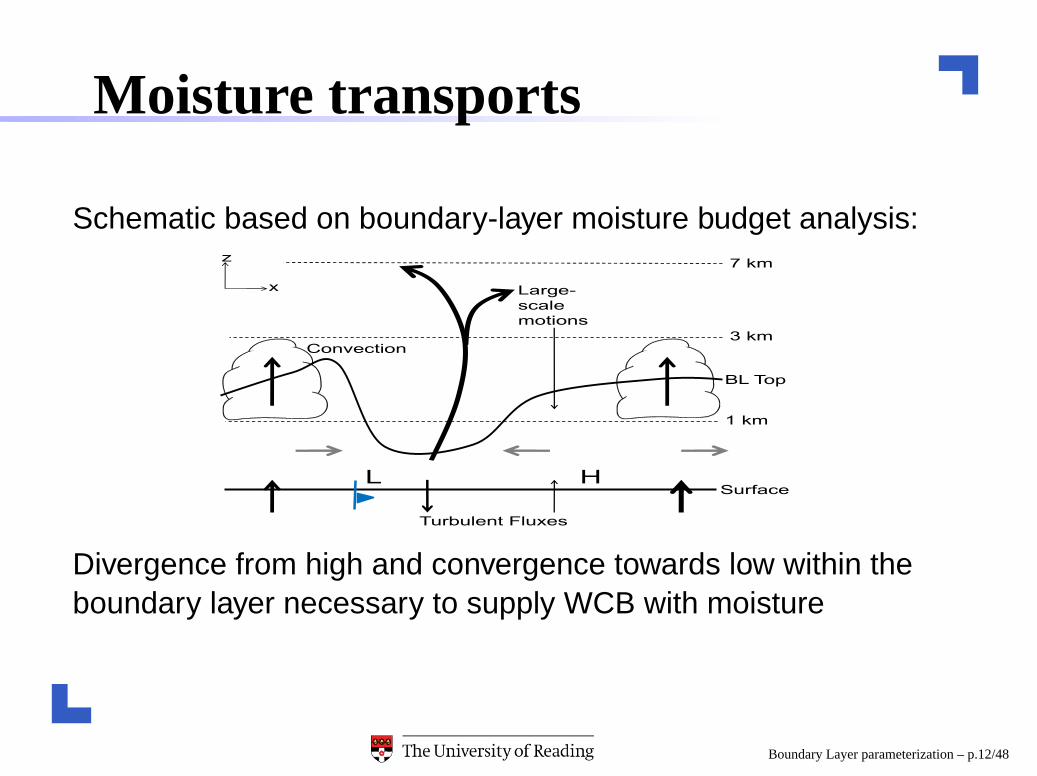
Moisture transports

Schematic based on boundary-layer moisture budget analysis:

Divergence from high and convergence towards low within theboundary layer necessary to supply WCB with moisture


Explicit turbulence simulations


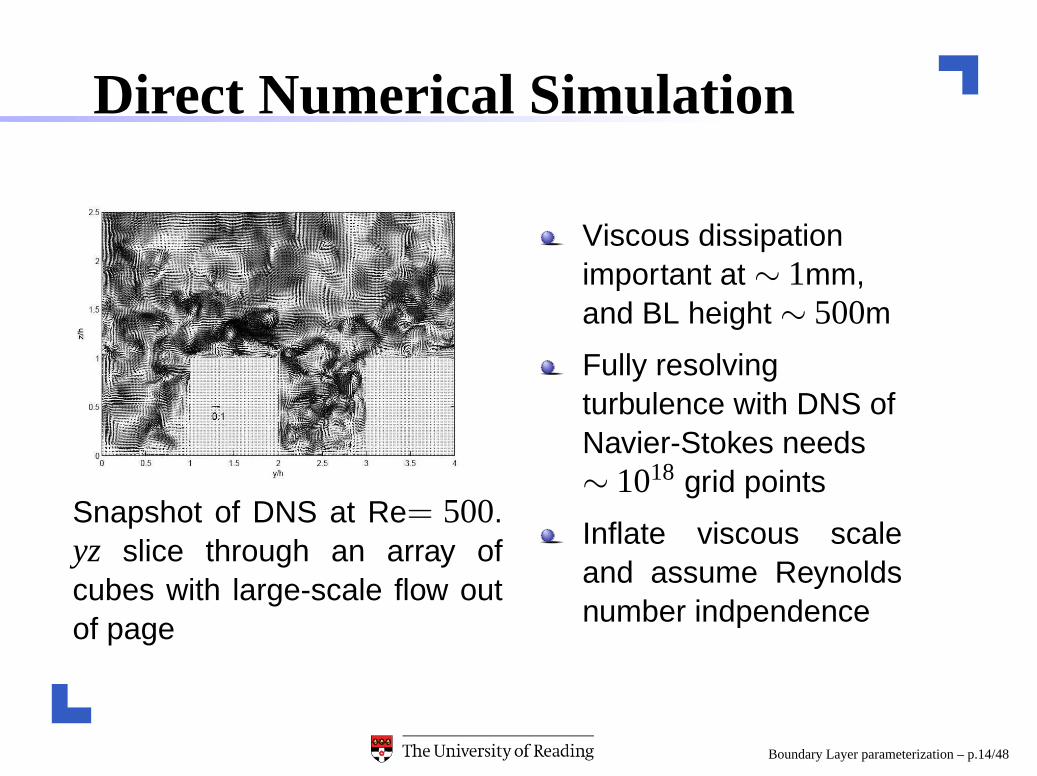
Direct Numerical Simulation

Snapshot of DNS at Re= 500.yz slice through an array ofcubes with large-scale flow outof page

Viscous dissipationimportant at ∼ 1mm,and BL height ∼ 500m

Fully resolvingturbulence with DNS ofNavier-Stokes needs∼ 1018 grid points

Inflate viscous scaleand assume Reynoldsnumber indpendence


Large Eddy Simulation

Simulate only as far as the inertial subrange: capture thelarge eddies

E =Z ∞

0E(k)dk ≈

Z kc=π/∆x

0E(k)dk

Dissipation rate is

ε = 2νZ ∞

0k2E(k)dk 6≈ 2ν

Z kc

0k2E(k)dk ≈ 0

Without viscous scales there is no sink of TKE


Energy loss from LES

Need a parameterization P of the energy drain

ε ≈ 2Z kc

0P(k)k2E(k)dk

Ideally P acts close to kc only so well-resolved eddies arenot affected

Popular (and very simple) choice is a Smagorinskyscheme, which is effectively a diffusion with coefficient∝ ∆x


LES snapshots ofw

CBL simulated at ∆x = ∆y = 10m, ∆z = 4m

z = 80m (left) and 800m (right)


Organization of the problem


NWP and GCMs: Closure Problem

On an NWP grid, no attempt to simulate turbulent eddies

Parameterize full turbulent spectrum.

∂u∂t

+u∂u∂x

+v∂u∂y

+w∂u∂z

− f v+1ρ

∂p∂x

=−∂u′u′

∂x−

∂v′u′

∂y−

∂w′u′

∂z

Effects of turbulence are described by fluxes like u′w′

Evolution equation for u′w′ includes u′w′w′ etc


Mellor-Yamada hierachy

Level 4 Carry (simplified) prognostic equations for all 2nd ordermoments with parameterization of 3rd order terms

Level 3 Carry (simplified) prognostic equations for θ′2 and TKEwith parameterization of 3rd order terms

Level 2.5 Carry (simplified) prognostic equation for TKE withparameterization of 3rd order terms

Level 2 Carry diagnostic equations for all 2nd order moments

Level 1 Carry simplified diagnostic equations 2nd order moments,K theory


Level 3

∂e∂t

= −u′w′∂u∂z

+gθ0

w′θ′−1ρ

∂∂z

w′p′−∂∂z

w′e− ε

∂θ′2

∂t= −2w′θ′

∂θ∂z

−∂∂z

w′θ′2− εθ

NWP/GCMs usually have diagnostic treatment but someuse TKE approach

Drop terms in red to get to the level 2.5, TKE approach

Not well justified theoretically though: no fundamentalreason to prefer kinetic to potential energy


Parameterization of terms

After Kolmogorov,

ε =eτ

∝e3/2

lεθ ∝

θ′2e1/2

l

Terms involving pressure treated using return-to-isotropyideas (Rotta)

Many possibilities for 3rd order terms, from simpledowngradient forms: eg,

w′u′2 ∝ −∂u′2

∂z

to much more “sophisticated” (ie, complicated!) methodsBoundary Layer parameterization – p.22/48

Surface layer parameterization


Surface Layer Similarity

Similarity theory requires us to:

1. write down all of physically relevant quantities that webelieve may control the strength and character of theturbulence

2. put these together into dimensionless combinations

3. any non-dimensional turbulent quantity must be a functionof the dimensionless variables: we just need to measurethat function


Monin-Obukhov theory: Step 1

Postulate that surface layer turbulence can be described by

height z

friction velocity (essentially the surface drag)

u∗ =

√

−u′w′0

a temperature scale that we can get from the surface heatflux

T∗ =w′θ′

0

u∗which is more conveniently expressed as a turbulentproduction of buoyancy (g/θ0)T∗



Construct dimensionless combinations from these three. Herez/L where L is the Obukhov length

L =−u2

∗θ0

kgT∗

L measures relative strength of shear and buoyancy

buoyancy becomes as important as shear at height z ∼ |L|

+ve in stable conditions

k is von Karman’s constant, = 0.4



Express the variables we need in terms of dimensionlessquantities

∂u∂z

=u∗kz

φm ;∂θ∂z

=T∗kz

φh

Now measure the dimensionless functions (obs or LES)

Which must be universal if the scaling is correct


Monin-Obukhov Theory: Step 3

Functions φm (left) and φh (right)


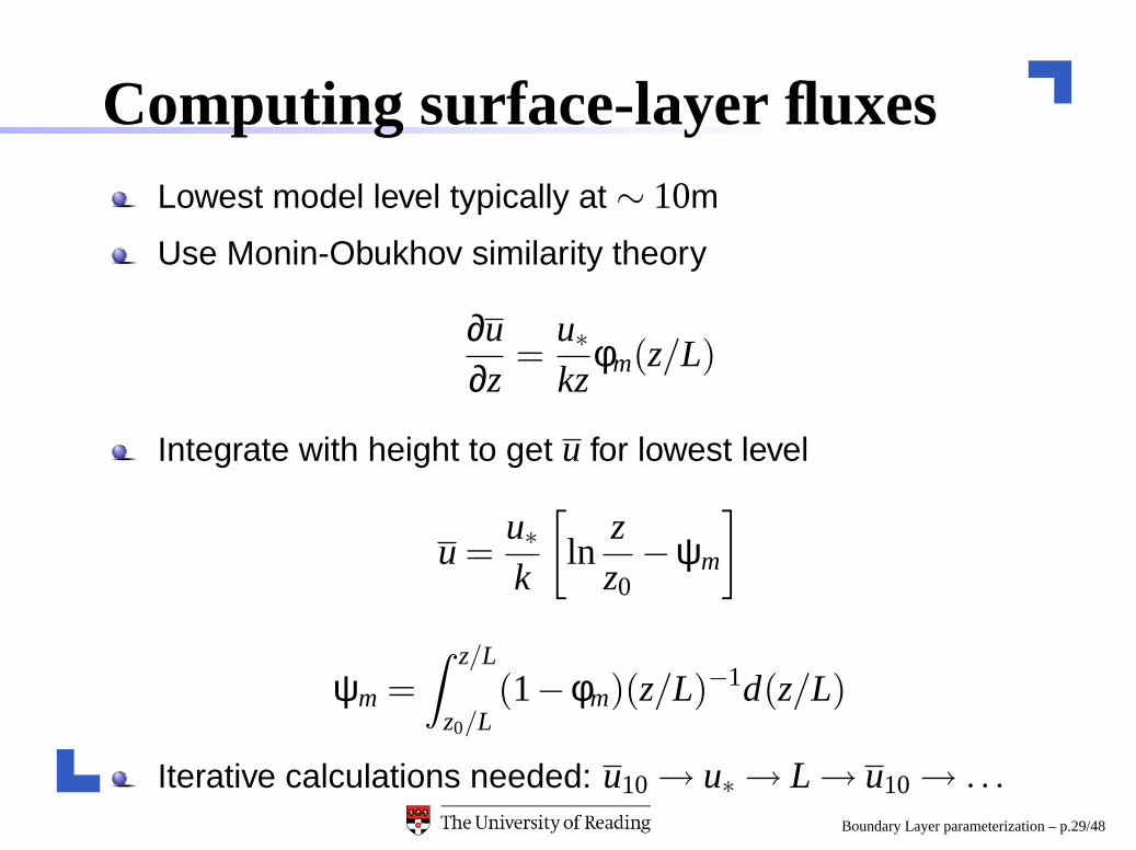
Computing surface-layer fluxesLowest model level typically at ∼ 10m

Use Monin-Obukhov similarity theory

∂u∂z

=u∗kz

φm(z/L)

Integrate with height to get u for lowest level

u =u∗k

[

lnzz0

−ψm

]

ψm =Z z/L

z0/L(1−φm)(z/L)−1d(z/L)

Iterative calculations needed: u10 → u∗ → L → u10 → . . .Boundary Layer parameterization – p.29/48

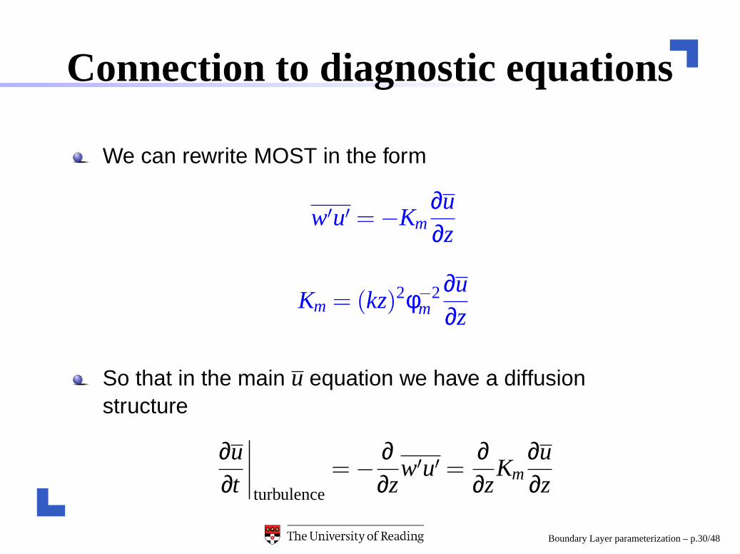
Connection to diagnostic equations

We can rewrite MOST in the form

w′u′ = −Km∂u∂z

Km = (kz)2φ−2m

∂u∂z

So that in the main u equation we have a diffusionstructure

∂u∂t

∣

∣

∣

∣

turbulence

= −∂∂z

w′u′ =∂∂z

Km∂u∂z


The outer boundary layer


Mixed Layer Similarity: Step 1

Surface heat flux w′θ′0 drives convective eddies of the

scale of h

Scaling velocities for vertical velocity and temperature

w∗ =

[

gθ0

w′θ′0h

]1/3

θ∗ =w′θ′

0

w∗

Dimensionless quantity z/h


Mixed Layer Similarity: Step 2

w′2 = w2∗ f1(z/h)

u′2 = w2∗ f2(z/h)

θ′2 = θ2∗ f3(z/h)

w′θ′ = w∗θ∗ f4(z/h)

ε =w3∗

hf5(z/h)

etc


Mixed layer similarity: Step 3

Left to right: w′2, u′2, θ′2, w′θ′, ε


K theoryFor the turbulent fluxes within the boundary layer, theK-theory formula is

w′u′ = −Km∂u∂z

Km = λ2m fm(Ri)

∂u∂z

compare Km = (kz)2φ−2m

∂u∂z

ie, generalizes MOST

Typical eddy size ∼ kz or λm

1λm

=1kz

+1l

where l ∝ h


Stability dependencez/L and Richardson number Ri play similar role inmeasuring relative importance of buoyancy and shear

Ri =− g

θ0

∂θ∂z

(∂u∂z

)2

The flux Richardson number is sometimes used instead

R f =−(g/θ0)w′θ′

w′θ′ ∂u∂z

ratio of terms in TKE equation


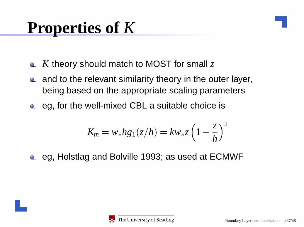
Properties of K

K theory should match to MOST for small z

and to the relevant similarity theory in the outer layer,being based on the appropriate scaling parameters

eg, for the well-mixed CBL a suitable choice is

Km = w∗hg1(z/h) = kw∗z(

1−zh

)2

eg, Holstlag and Bolville 1993; as used at ECMWF


A problem in the CBL

w′θ′ = −Kh∂θ∂z

=⇒ can diagnose Kh from LES/obs data


A solution for the CBL

Simplest possibility is to introduce a non-local contribution

w′θ′ = −Kh∂θ∂z

+Khγ

where γ is simply a number


Parameterizations Based on Scalings

Possible difficulties are:

Developing good scalings for each boundary layer regime

Good decison making needed for which regime to apply

Handling transitions between regimes


Effects of radiation on buoyancy

LW cooling at cloud top; SW heating within cloudproduces source of buoyant motions


UM scheme

Decision making about type is important

Sc treated as BL cloud; shallow Cu separately


EDMFEddy-diffusivity mass-flux treatment,w′φ′ = −Kdφ/dz+∑i Mi(φi −φ)

Mass flux component for largest, most energetic eddies ofsize ∼ h which produce the non-local transport

Can be used as a treatment for Sc and (especially)shallow Cu

Can be high sensitivity to bulk entrainment rate


The boundary layer grey zone


The grey zone

NWP approaches to turbulence valid when all turbulenceis parameterized

LES approaches to turbulence valid

Grey zone is difficult middle range when model grid iscomparable to the size of energy-containing eddies

Should we try to ignore or such eddies and use an NWPapproach? Double counting?

Or allow them and use an LES approach? Risks undercounting?


A Perspective from LESStochastic backscatter useful very near surface where∆ ≪ l breaks down

eg, improves profiles of dimensionless wind shear nearsurface

Other LES models proposed for grey zone: dynamicmodel, tensorial model...

Dry, neutral boundary layer, Weinbrecht 2006


Perspective from NWPSmall boundary layer fluctuations (∼ 0.1K) important forconvective initiation

Can easily shift the locations of precipitating cells e.g.

Leoncini et al (2010)

Perturbation at 2000 UTC, 8 km

K

−0.1

−0.05

0

0.05

0.1

0 2 4 6 8 10 12 14 16 18 200

0.1

0.2

0.3

0.4

0.5

0.6

0.7

0.8

0.9

1

Time UTC

Fra

ctio

n

Raining in perturbedRaining in control

Raining in both


Conclusions

Most NWP models have relatively simple turbulencemodelling based on K-theory

Simple methods are able to make use of similarityarguments

These often work very well in the appropriate regimes,although transitions between regimes can be awkwardand somewhat ad hoc

...because the performance is not very much worse thanusing very much more complex and more expensiveturbulence modelling approaches

But as resolutions ∆x → h new approaches may beneeded; ensemble-based modelling breaks down


bob plant - university of readingsws00rsp/teaching/nanjing/blayer.pdf · outline motivation some...

Documents