book of modules for the elite master's programme

Book of Modules for the Elite Master’s Programme

Scientific Computing

Faculty for Mathematics, Physics and Computer Science, University of Bayreuth, Germany

March 11, 2021

Preface

This Book of Modules describes all currently admissible modules for the elite master’s programme Scientific Computing andtheir assignment to the module areas decribed in the examination regulations ”Studien- und Prufungsordnung”. Each moduledescription contains the frequency (and sometimes the term) with which the corresponding course is offered; the list of coursesactually provided during the current semester is published via Campus Online. The coordinator of this master’s programme willbe glad to help you selecting suitable courses to satisfy the requirements formulated in the examination regulations.

The executive committee of the elite master’s programme March 11, 2021

Contents

1 Module Section A: Numerical Mathematics 31.1 Module A1: Numerical Methods for Differential Equations . . . . . . . . . . . . . . . . . . . . . . . . . . . . . . . 3

1.2 Elective Modules A2: Advanced Topics in Numerical Mathematics . . . . . . . . . . . . . . . . . . . . . . . . . . 4

2 Module Section B: Modeling and Simulation 102.1 Module B1: Applied Functional Analysis . . . . . . . . . . . . . . . . . . . . . . . . . . . . . . . . . . . . . . . . 10

2.2 Elective Modules B2: Modeling and Simulation . . . . . . . . . . . . . . . . . . . . . . . . . . . . . . . . . . . . 11

2.3 Module B3: Industrial Internship . . . . . . . . . . . . . . . . . . . . . . . . . . . . . . . . . . . . . . . . . . . . 23

2.4 Module B4: Modeling and Status Seminar . . . . . . . . . . . . . . . . . . . . . . . . . . . . . . . . . . . . . . . 25

3 Module Section C: High-Performance Computing 263.1 Elective Modules C1: High-Performance Computing . . . . . . . . . . . . . . . . . . . . . . . . . . . . . . . . . 26

3.2 Module C2: Practical Course on Parallel Numerical Methods . . . . . . . . . . . . . . . . . . . . . . . . . . . . . 33

4 Module Section D: Scientific Computing 344.1 Elective Modules D1: Complexity Reduction . . . . . . . . . . . . . . . . . . . . . . . . . . . . . . . . . . . . . . 34

4.2 Module D2: Special Skills in Scientific Computing . . . . . . . . . . . . . . . . . . . . . . . . . . . . . . . . . . . 44

5 Module Section E: Soft Skills 45

6 Module Section F: Master’s Thesis 46

7 Recommended Curriculum 47

2

1 Module Section A: Numerical Mathematics

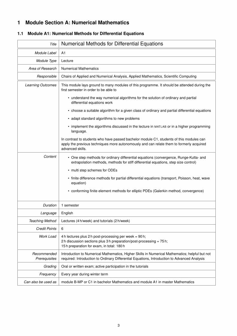
1.1 Module A1: Numerical Methods for Differential Equations

Title Numerical Methods for Differential Equations

Module Label A1

Module Type Lecture

Area of Research Numerical Mathematics

Responsible Chairs of Applied and Numerical Analysis, Applied Mathematics, Scientific Computing

Learning Outcomes This module lays ground to many modules of this programme. It should be attended during thefirst semester in order to be able to

• understand the way numerical algorithms for the solution of ordinary and partialdifferential equations work

• choose a suitable algorithm for a given class of ordinary and partial differential equations

• adapt standard algorithms to new problems

• implement the algorithms discussed in the lecture in MATLAB or in a higher programminglanguage.

In contrast to students who have passed bachelor module C1, students of this modules canapply the previous techniques more autonomously and can relate them to formerly acquiredadvanced skills.

Content • One step methods for ordinary differential equations (convergence, Runge-Kutta- andextrapolation methods, methods for stiff differential equations, step size control)

• multi step schemes for ODEs

• finite difference methods for partial differential equations (transport, Poisson, heat, waveequation)

• conforming finite element methods for elliptic PDEs (Galerkin method, convergence)

Duration 1 semester

Language English

Teaching Method Lectures (4 h/week) and tutorials (2 h/week)

Credit Points 6

Work Load 4 h lectures plus 2 h post-processing per week = 90 h;2 h discussion sections plus 3 h preparation/post-processing = 75 h;15 h preparation for exam, in total: 180 h

RecommendedPrerequisites

Introduction to Numerical Mathematics, Higher Skills in Numerical Mathematics; helpful but notrequired: Introduction to Ordinary Differential Equations, Introduction to Advanced Analysis

Grading Oral or written exam; active participation in the tutorials

Frequency Every year during winter term

Can also be used as module B-MP or C1 in bachelor Mathematics and module A1 in master Mathematics

3

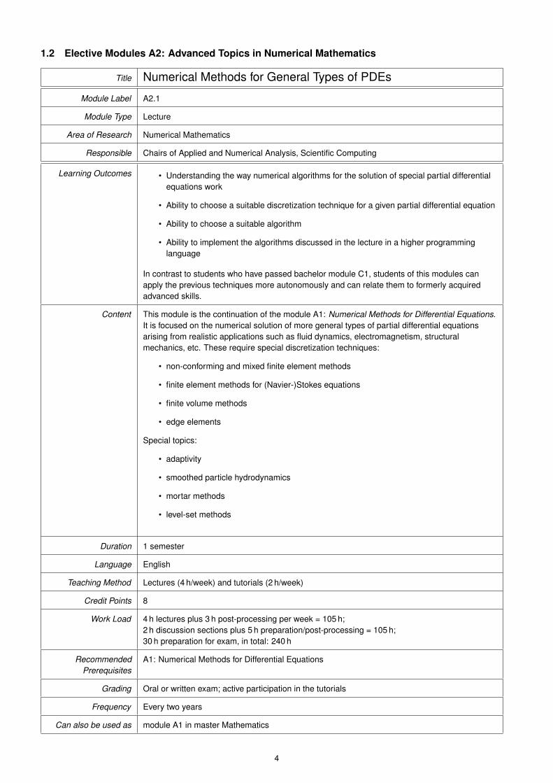
1.2 Elective Modules A2: Advanced Topics in Numerical Mathematics

Title Numerical Methods for General Types of PDEs

Module Label A2.1

Module Type Lecture


Responsible Chairs of Applied and Numerical Analysis, Scientific Computing

Learning Outcomes • Understanding the way numerical algorithms for the solution of special partial differentialequations work

• Ability to choose a suitable discretization technique for a given partial differential equation

• Ability to choose a suitable algorithm

• Ability to implement the algorithms discussed in the lecture in a higher programminglanguage


Content This module is the continuation of the module A1: Numerical Methods for Differential Equations.It is focused on the numerical solution of more general types of partial differential equationsarising from realistic applications such as fluid dynamics, electromagnetism, structuralmechanics, etc. These require special discretization techniques:

• non-conforming and mixed finite element methods

• finite element methods for (Navier-)Stokes equations

• finite volume methods

• edge elements

Special topics:

• adaptivity

• smoothed particle hydrodynamics

• mortar methods

• level-set methods

Duration 1 semester

Language English


Credit Points 8



A1: Numerical Methods for Differential Equations


Frequency Every two years

Can also be used as module A1 in master Mathematics

4

Title Discontinuous Galerkin Finite Element Methods

Module Label A2.2

Module Type Lecture


Responsible Chair of Scientific Computing

Learning Outcomes • Understanding of important analysis techniques for Sobolev spaces and theirmodifications for discontinuous approximation spaces

• Ability to choose and apply a suitable discontinuous Galerkin discretization for standardlinear and nonlinear advection–diffusion problems

• Ability to implement various types of discontinuous Galerkin discretizations in 1D and 2Dusing a programming language

Content This course introduces the DG methods for hyperbolic and parabolic partial differential equations(PDEs) and systems of PDEs; it includes formulations for one- and multi-dimensional domains,for linear and nonlinear equations, and considers the stability and convergence analysis forthese formulations. Also more advanced topics such as hybridized and ADER-DG methods aswell as Riemann problems and their solution constitute a subject of this course.

Duration 1 semester

Language English


Credit Points 4

Work Load 2 h lectures plus 1,5 h post-processing per week = 52,5 h;1 h discussion sections plus 2,5 h preparation/post-processing = 52,5 h;15 h preparation for exam; in total: 120 h


A1: Numerical Methods for Differential Equations, B1: Applied Functional Analysis


Frequency Every year

Can also be used as module B1 in master Mathematics

5

Title Constructive Approximation Methods

Module Label A2.3

Module Type Lecture

Area of Research Advanced Analysis and Applications / Numerical Mathematics

Responsible Chair of Applied and Numerical Analysis

Learning Outcomes By the end of the course, a successful student should be able to

• explain the most important concepts of modern, multivariate approximation methods

• explain the problems inherent to the reconstruction of multivariate functions fromscattered data

• prove and analyse the existence, the uniqueness, the computability and the quality ofdiscrete reconstruction techniques

• explain and implement the associated numerical schemes

• understand the underlying mathematical theory


Content • Jackson- and Bernstein theorems for classical univariate polynomial approximation

• Multivariate reconstruction methods based upon radial basis functions, movingleast-squares and partition of unity methods

• Error and stability analysis of multivariate reconstruction methods

• Development and implementation of efficient algorithms for such reconstruction methods

• Optimal recovery for generalised interpolation with application to solving partial differentialequations

Duration 1 semester

Language English


Credit Points 8



Introduction to Advanced Analysis, Introduction to Numerical Mathematics




6

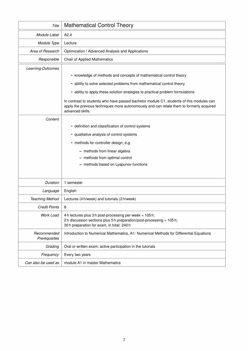
Title Mathematical Control Theory

Module Label A2.4

Module Type Lecture

Area of Research Optimization / Advanced Analysis and Applications

Responsible Chair of Applied Mathematics

Learning Outcomes

• knowledge of methods and concepts of mathematical control theory

• ability to solve selected problems from mathematical control theory

• ability to apply these solution strategies to practical problem formulations


Content

• definition and classification of control systems

• qualitative analysis of control systems

• methods for controller design, e.g.

– methods from linear algebra

– methods from optimal control

– methods based on Lyapunov functions

Duration 1 semester

Language English


Credit Points 8



Introduction to Numerical Mathematics, A1: Numerical Methods for Differential Equations




7

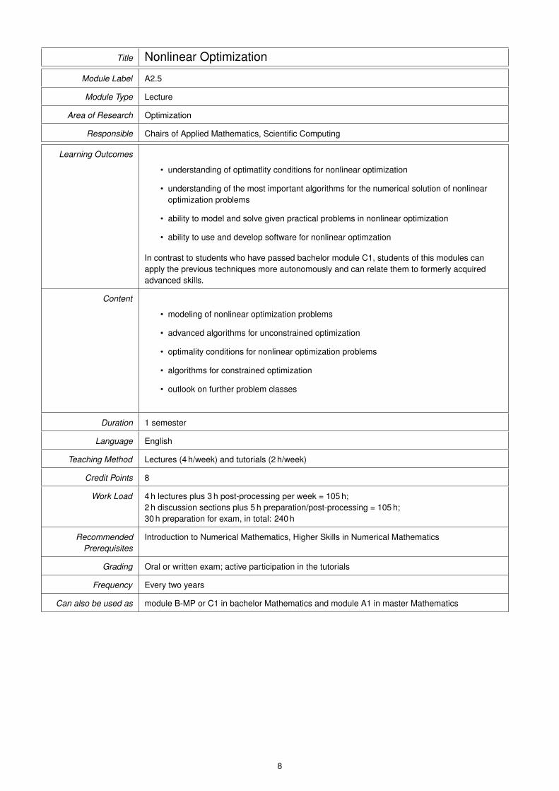
Title Nonlinear Optimization

Module Label A2.5

Module Type Lecture

Area of Research Optimization

Responsible Chairs of Applied Mathematics, Scientific Computing

Learning Outcomes

• understanding of optimatlity conditions for nonlinear optimization

• understanding of the most important algorithms for the numerical solution of nonlinearoptimization problems

• ability to model and solve given practical problems in nonlinear optimization

• ability to use and develop software for nonlinear optimzation


Content

• modeling of nonlinear optimization problems

• advanced algorithms for unconstrained optimization

• optimality conditions for nonlinear optimization problems

• algorithms for constrained optimization

• outlook on further problem classes

Duration 1 semester

Language English


Credit Points 8



Introduction to Numerical Mathematics, Higher Skills in Numerical Mathematics




8

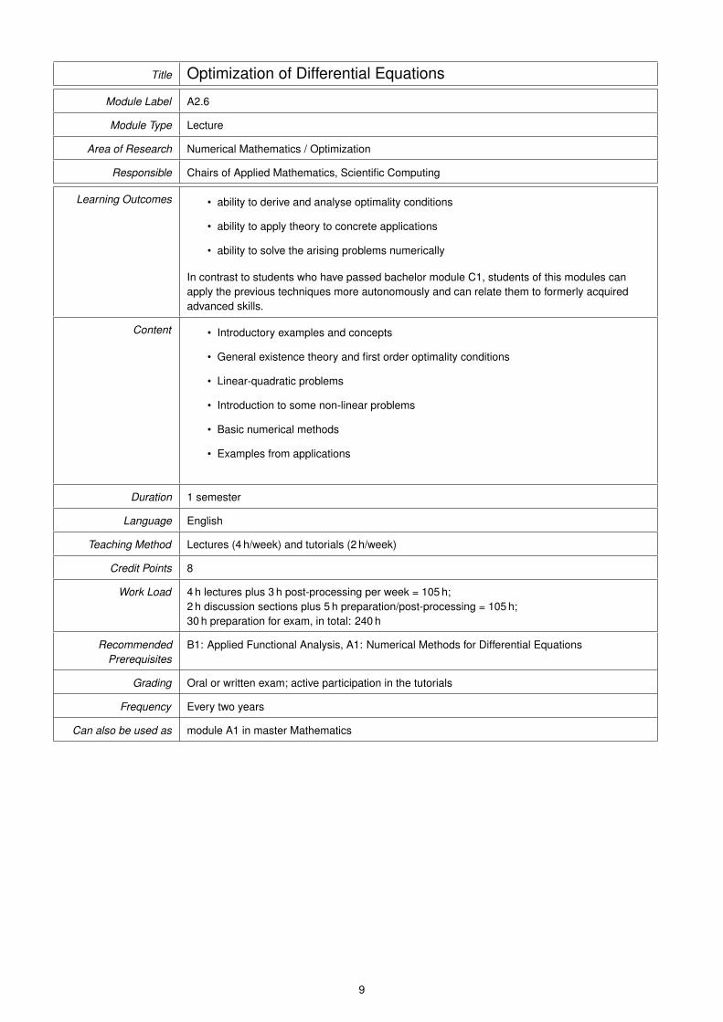
Title Optimization of Differential Equations

Module Label A2.6

Module Type Lecture

Area of Research Numerical Mathematics / Optimization


Learning Outcomes • ability to derive and analyse optimality conditions

• ability to apply theory to concrete applications

• ability to solve the arising problems numerically


Content • Introductory examples and concepts

• General existence theory and first order optimality conditions

• Linear-quadratic problems

• Introduction to some non-linear problems

• Basic numerical methods

• Examples from applications

Duration 1 semester

Language English


Credit Points 8



B1: Applied Functional Analysis, A1: Numerical Methods for Differential Equations




9

2 Module Section B: Modeling and Simulation

2.1 Module B1: Applied Functional Analysis

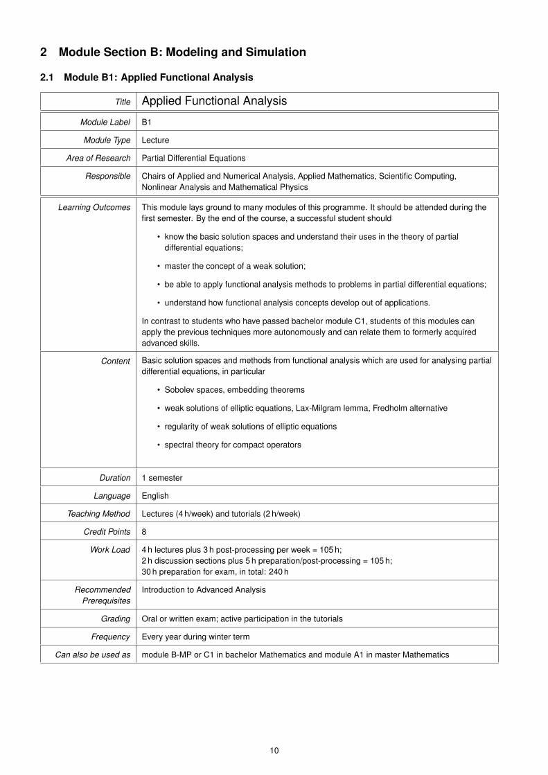
Title Applied Functional Analysis

Module Label B1

Module Type Lecture

Area of Research Partial Differential Equations

Responsible Chairs of Applied and Numerical Analysis, Applied Mathematics, Scientific Computing,Nonlinear Analysis and Mathematical Physics

Learning Outcomes This module lays ground to many modules of this programme. It should be attended during thefirst semester. By the end of the course, a successful student should

• know the basic solution spaces and understand their uses in the theory of partialdifferential equations;

• master the concept of a weak solution;

• be able to apply functional analysis methods to problems in partial differential equations;

• understand how functional analysis concepts develop out of applications.


Content Basic solution spaces and methods from functional analysis which are used for analysing partialdifferential equations, in particular

• Sobolev spaces, embedding theorems

• weak solutions of elliptic equations, Lax-Milgram lemma, Fredholm alternative

• regularity of weak solutions of elliptic equations

• spectral theory for compact operators

Duration 1 semester

Language English


Credit Points 8



Introduction to Advanced Analysis




10

2.2 Elective Modules B2: Modeling and Simulation

Title Partial Differential Equations and Integral Equations

Module Label B2.1

Module Type Lecture


Responsible Chair of Nonlinear Analysis and Mathematical Physics

Learning Outcomes By the end of the course, a successful student should

• understand the origin of the treated equations in the modeling process;

• know fundamental results on existence and uniqueness of their solutions;

• understand qualitative properties of their solutions;

• master key methods of their analysis.


Content Existence, uniqueness, and properties of solutions for integral equations and for various types ofpartial differential equations that are eminent for modeling in the sciences, in particular

• parabolic equations

• wave equations and symmetric hyperbolic systems

• Schrodinger equations

• integral operators related to elliptic equations

Duration 1 semester

Language English


Credit Points 8



Introduction to Advanced Analysis, B1: Applied Functional Analysis




11

Title Modeling with Differential Equations

Module Label B2.2

Module Type Lecture



Learning Outcomes • Ability to identify suitable mathematical models for a given application

• Knowledge about important modeling principles

• Ability to apply modeling techniques to basic practical applications


Content • General modeling principles

• Mathematical Models based on Ordinary Differential Equations from, e.g.,

– Mathematical Biology

– Mechanics

• Mathematical Models based on Partial Differential Equations from, e.g.,

– Mathematical Physics

– Mathematical Finance

Duration 1 semester

Language English


Credit Points 4

Work Load 2 h lectures plus 1.5 h post-processing per week = 52.5 h;1 h discussion sections plus 2.5 h preparation/post-processing = 52.5 h;15 h preparation for exam; in total: 120 h


B1: Applied Functional Analysis, A1: Numerical Methods for Differential Equations




12

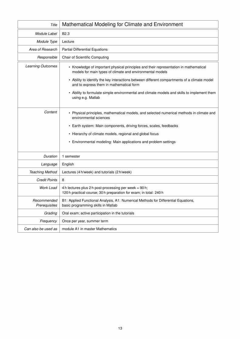
Title Mathematical Modeling for Climate and Environment

Module Label B2.3

Module Type Lecture



Learning Outcomes • Knowledge of important physical principles and their representation in mathematicalmodels for main types of climate and environmental models

• Ability to identify the key interactions between different compartments of a climate modeland to express them in mathematical form

• Ability to formulate simple environmental and climate models and skills to implement themusing e.g. Matlab

Content • Physical principles, mathematical models, and selected numerical methods in climate andenvironmental sciences

• Earth system: Main components, driving forces, scales, feedbacks

• Hierarchy of climate models, regional and global focus

• Environmental modeling: Main applications and problem settings

Duration 1 semester

Language English


Credit Points 8

Work Load 4 h lectures plus 2 h post-processing per week = 90 h;120 h practical course; 30 h preparation for exam; in total: 240 h


B1: Applied Functional Analysis, A1: Numerical Methods for Differential Equations,basic programming skills in Matlab

Grading Oral exam; active participation in the tutorials

Frequency Once per year, summer term


13

Title Pattern Recognition

Module Label B2.4

Module Type Lecture

Area of Research Computer Science

Responsible Chair of Applied Computer Science III

Learning Outcomes This course imparts advanced, systematic comprehension and methods to recognize or classifypatterns in a set of data. E. g. applications are in the fields of object recognition, recognition ofhand writing, speech, or gestures, and facial recognition.

Content Bayesian classification, Parameter estimation, Nonparametric techniques, Linear classification,Feedforward neural networks, Feedback neural networks, Nonmetric methods, SupervisedLearn- ing, Unsupervised Learning

Duration 1 semester

Language English


Credit Points 4



none

Grading Oral exam

Frequency Once per year, winter term

Can also be used as

14

Title Mechanics of Continua

Module Label B2.5

Module Type Lecture

Area of Research Fluid Mechanics

Responsible Theoretical Physics

Learning Outcomes • Understand fundamental concepts of continuum mechanics such as stress tensors,dynamic equations

• Assess which physical effects are relevant/irrelevant for a given situation

• Propose a theoretical description and solution approach for a given continuum mechanicalproblem

Content • Fundamental concepts in fluid mechanics: pressure, stress tensor

• Euler, Stokes and Navier-Stokes equations

• Dimensionless numbers

• Applications to

– Turbulence

– Microfluids

Duration 1 semester

Language German / English on demand


Credit Points 8

Work Load 4 h lectures plus 3 h post-processing per week = 105 h;2 h discussion sections plus 5 h preparation/post-processing = 105 h;30 h preparation for exam; in total: 240 h


Understanding of classical Newtonian mechanics

Grading Oral or written exam


Can also be used as

15

Title Molecular Dynamics Simulations of Biophysical Systems

Module Label B2.6

Module Type Lecture

Area of Research Physics

Responsible Biofluid Simulation and Modeling

Learning Outcomes • Understanding of the theoretical background in biophysical simulations

• Practical application to example problems, e.g. protein folding

Content Molecular Dynamics computer simulations have become an invaluable tool in many areas of thenatural sciences. Their widespread applications range from protein folding and membranedynamics in biological physics, solute-solvent interactions in theoretical chemistry to nanofluidicsin process engineering. The aim of this course is (i) to understand the physics behind frequentlyemployed simulation methods and (ii) to gain practical experience in using these methods for arange of sample prob-lems. We will start by considering the basic ingredients for atomisticsimulations such as Verlet integration, force fields, long-range electrostatistic interactions,thermostating, etc. We will then move on to cover more advanced topics such as free energymethods and sampling techniques for rare events. Finally, we will discuss systematiccoarse-graining methods which allow the simulation of larger and more complicated processes,e.g. the unfolding of a protein in shear flow. The course includes a lab part in which actualsimulations with the GROMACS package are conducted.

Duration 1 semester

Language English

Teaching Method Lectures (2 h/week) and additional practical project

Credit Points 4

Work Load 2 h lectures plus 2 h post-processing per week = 60 h;Practical project = 40 h;20 h preparation for exam; in total: 120 h


Knowledge of statistical mechanics is helpful


Frequency Approximately every two years

Can also be used as

16

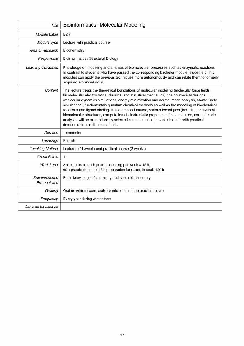
Title Bioinformatics: Molecular Modeling

Module Label B2.7

Module Type Lecture with practical course

Area of Research Biochemistry

Responsible Bioinformatics / Structural Biology

Learning Outcomes Knowledge on modeling and analysis of biomolecular processes such as enzymatic reactionsIn contrast to students who have passed the corresponding bachelor module, students of thismodules can apply the previous techniques more autonomously and can relate them to formerlyacquired advanced skills.

Content The lecture treats the theoretical foundations of molecular modeling (molecular force fields,biomolecular electrostatics, classical and statistical mechanics), their numerical designs(molecular dynamics simulations, energy minimization and normal mode analysis, Monte Carlosimulations), fundamentals quantum chemical methods as well as the modeling of biochemicalreactions and ligand binding. In the practical course, various techniques (including analysis ofbiomolecular structures, computation of electrostatic properties of biomolecules, normal-modeanalysis) will be exemplified by selected case studies to provide students with practicaldemonstrations of these methods.

Duration 1 semester

Language English

Teaching Method Lectures (2 h/week) and practical course (3 weeks)

Credit Points 4



Basic knowledge of chemistry and some biochemistry

Grading Oral or written exam; active participation in the practical course


Can also be used as

17

Title Foundations of Bioinformatics

Module Label B2.8

Module Type Lecture with practical course

Area of Research Biochemistry

Responsible Bioinformatics / Structural Biology

Learning Outcomes Students should acquire the basics of bioinformatics and get to know them in theory andpractice.In contrast to students who have passed the corresponding bachelor module, students of thismodules can apply the previous techniques more autonomously and can relate them to formerlyacquired advanced skills.

Content The lecture covers the basic bioinformatic applications. Namely, the application of varioustheoretical methods in the analysis of molecular biological data in the foreground (databasesand database search, sequences and sequence alignments, phylogenetic trees) as well asfundamentals of molecular modeling, structure prediction and drug design. In the practicalcourse, the students have hands-on sessions for the different methods, the use of internet toolsfor sequence data analysis, web-based databases and creation of sequence alignments.Moreover some basic introduction to molecular visualization and an introduction to the UNIXoperating system are provided.

Duration 1 semester

Language German

Teaching Method Lectures (2 h/week) and practical course (3 h/week)

Credit Points 4

Work Load 2 h lectures plus 2 h post-processing per week = 60 h3 h practical course = 45 h; 15 h preparation for exam; in total: 120 h


Basic knowledge of chemistry and some biochemistry


Frequency Every year during summer term

Can also be used as

18

Title Higher Strengths of Materials

Module Label B2.9

Module Type Lecture

Area of Research Engineering Science

Responsible Chair of Design and CAD

Learning Outcomes The module enables the students to calculate complex technical products by use of linearelasticity approach. It deepens the knowledge in the area of strengths of materials calculation.In contrast to students who have passed the corresponding bachelor module, students of thismodules can apply the previous techniques more autonomously and can relate them to formerlyacquired advanced skills.

Content Selected subjects in higher strengths of materials area, e.g. multiaxial stress and deformation,theories of thin shells, mechanical vibrations with relation to typical applications.

Duration 1 semester

Language German


Credit Points 4



Basic engineering knowledge funding on Bachelor Engineering Science studies, especially intechnical mechanics and strengths of materials.

Grading Written examination (60 min)


Can also be used as

19

Title Computer Aided Engineering

Module Label B2.10

Module Type Lecture



Learning Outcomes CAE1: ability to create CAD models and generate design proposals using optimizationalgorithms.CAE2: mastery of modern methods of calculation of statics and their application to constructivetasks; knowledge of associated softwareIn contrast to students who have passed the corresponding bachelor module, students of thismodules can apply the previous techniques more autonomously and can relate them to formerlyacquired advanced skills.

Content CAE1: mastery of modern calculation methods and their application to constructive tasks;knowledge of associated software. Ability to design independently using CAD.CAE2: theory and application of finite element methods to static problems with a focus on theconstructive point of view and modeling.

Duration 2 semesters

Language English

Teaching Method CAE1: lectures (2 h/week) and CAE2: seminar (2 h/week)

Credit Points 4

Work Load 2 h lectures plus 1.5 h post-processing per week = 52.5 h;2 h seminar plus 1.5 h preparation/post-processing = 52.5 h;15 h preparation for exam; in total: 120 h


Basic technical understandingA1: Numerical Methods for Differential Equations

Grading Written examination; For the admission to the written exam a vivid participation in the exercisesis required.


Can also be used as

20

Title Model Building and Simulation of Mechanical Systems

Module Label B2.11

Module Type Lecture



Learning Outcomes The industrial standard CAD software CATIA enables students to create virtual models ofproducts. The course Higher Finite Element Analysis enables students to build-up models forthe dimensioning of complex technical products by use of sophisticated Finite Element Analysismethods. The knowledge is used in wide areas of advanced product development.In contrast to students who have passed the corresponding bachelor module, students of thismodules can apply the previous techniques more autonomously and can relate them to formerlyacquired advanced skills.

Content FEA: Handling of great and complex structures, use of shell and volume elements. Solvingnon-linearity, vibration and heat transfer problems.CATIA: Part and assembly creation; generation of technical drawings; surface modeling withGenerative Shape Design.


Language German

Teaching Method FEA: lectures (2 h/week), seminar (1 h/week) and CATIA: seminar (2 h/week)

Credit Points 6

Work Load FEA:45 h lecture + follow up work45 h seminars + preparation and follow-up work

CATIA:60 h seminars + preparation and follow-up work

Examination: 30 h examination preparation; Module in total: 180 hours


Basic engineering knowledge funding on Bachelor Engineering Science studies, especially intechnical mechanics, construction design and mechanical engineering

Grading Written examination (120 min)


Can also be used as

21

Title Foundations of Data Management

Module Label B2.12

Module Type Lecture

Area of Research Data Management, Data Science

Responsible Chair of Theoretical Computer Science

Learning Outcomes Students will learn the mathematical foundations of data management (which includesdatabases and data science). They will understand the connections between logic, expressivity,computational complexity, and efficient algorithms in this area. They will learn the formal tools tobe able to understand and interpret recent scientific developments in the area.

Content The lecture starts with formal definitions of databases and query languages. After showing thatthere is a deep connection between first-order logic and SQL when it comes to queryingrelational databases, it investigates the computational complexity (or efficient algorithms) forevaluating and analyzing SQL or first-order logic queries on databases. We then investigateconjunctive queries as a practically relevant special case, treat their evaluation and optimizationproblems, and connections with graph theory. (Knowledge of SQL is helpful but is not required.)

Duration 1 semester

Language English


Credit Points 4

Work Load 2 h lectures plus 1.5 h post-processing per week = 52.5 h;1 h exercises plus 1 h post-processing per week = 30 h;37.5 h preperation for the exam; in total: 120 h


Theoretische Informatik 1 or mathematical skills equivalent to those obtained in a BSc degree inmathematics or physics

Grading Oral or written exam; participation in the tutorials


Can also be used as

22

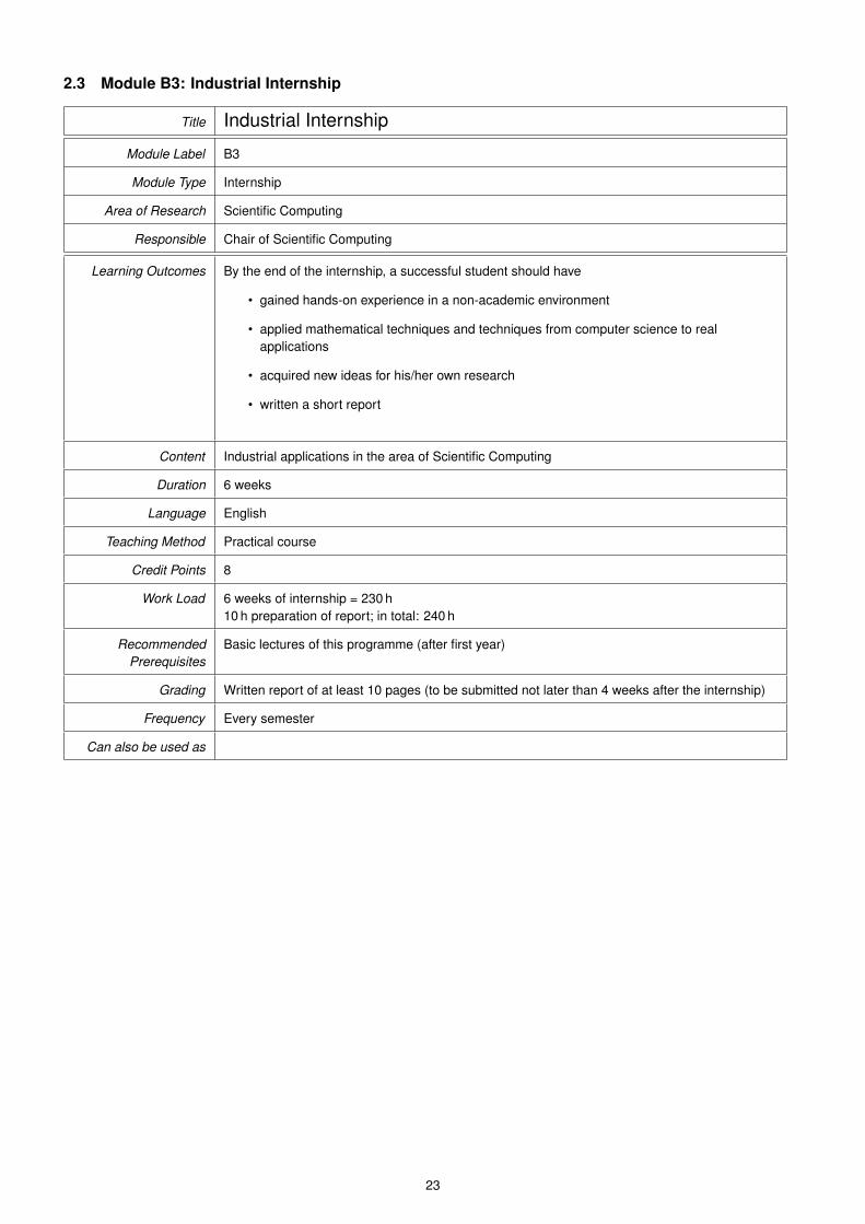
2.3 Module B3: Industrial Internship

Title Industrial Internship

Module Label B3

Module Type Internship

Area of Research Scientific Computing


Learning Outcomes By the end of the internship, a successful student should have

• gained hands-on experience in a non-academic environment

• applied mathematical techniques and techniques from computer science to realapplications

• acquired new ideas for his/her own research

• written a short report

Content Industrial applications in the area of Scientific Computing

Duration 6 weeks

Language English

Teaching Method Practical course

Credit Points 8

Work Load 6 weeks of internship = 230 h10 h preparation of report; in total: 240 h


Basic lectures of this programme (after first year)

Grading Written report of at least 10 pages (to be submitted not later than 4 weeks after the internship)

Frequency Every semester

Can also be used as

23

2.4 Module B4: Modeling and Status Seminar

Title Modeling and Status Seminar

Module Label B4

Module Type Seminar

Area of Research All areas


Learning Outcomes Successful students can

• Modeling and numerical solution:transfer real-world problems to a mathematical modelpave their way into a scientific topic; work in small groupsselect suitable efficient numerical methods and implement them on parallel computers

• Talk:choose and master suitable presentation techniquesspeak freely about a subject and illustrate important structures instructivelyanswer spontaneous questions from the audience in a reliable manner

• Discussion:phrase appropriate subject-specific questionsexpress constructive criticism for a talkexploit constructive criticism for their future talks

• Handout:expose an advanced mathematical subject briefly, concisely, and memorably in writingefficient usage of scientific publication systems (e.g., LATEX)

Content Modeling Seminar:

• Students receive real-world projects and work (in small groups) their way into them

• Each group prepares a presentation for its subject (duration: 30–60 minutes) and talksabout it in front of the plenum

• Each group prepares and distributes a report (at least 10 pages) using a scientific textsystem (e.g., LATEX)

Status Seminar:

• Each student prepares a presentation on the status of his/her studies and results ofhis/her research (duration: 15–30 minutes) and talks about it in front of the plenum

For both seminars there will be a discussion on the subject and on the presentation.


Language English

Teaching Method Modeling seminar (1 week) and status seminar (2 days) each year

Credit Points 8

Work Load 70 h practical course and 30 h seminar each year = 200 h40 h preparation/post-processing for seminar, in total: 240 h


At least one module of A2 and D1, respectively; C2: Practical Course on Parallel NumericalMethods

Grading Oral presentation and written report of at least 10 pages (to be submitted not later than 4 weeksafter the seminar)

Frequency Each year (modeling seminar during summer break, status seminar during winter break)

Can also be used as

25

3 Module Section C: High-Performance Computing

3.1 Elective Modules C1: High-Performance Computing

Title Algorithms and Data Structures II

Module Label C1.1

Module Type Lecture


Responsible Chair of Algorithms and Data Structures

Learning Outcomes This module teaches advanced techniques for the design and analysis of algorithms and datastructures.In contrast to students who have passed the corresponding bachelor module, students of thismodules can apply the previous techniques more autonomously and can relate them to formerlyacquired advanced skills.

Content Possible topics are:

• design principles

• graph algorithms

• advanced data structures

• approximation algorithms

• parameterized algorithms

• randomized algorithms

Duration 1 semester

Language English


Credit Points 8



Elementary programming skills, Basic skills in the design and analysis of algorithms.



Can also be used as

26

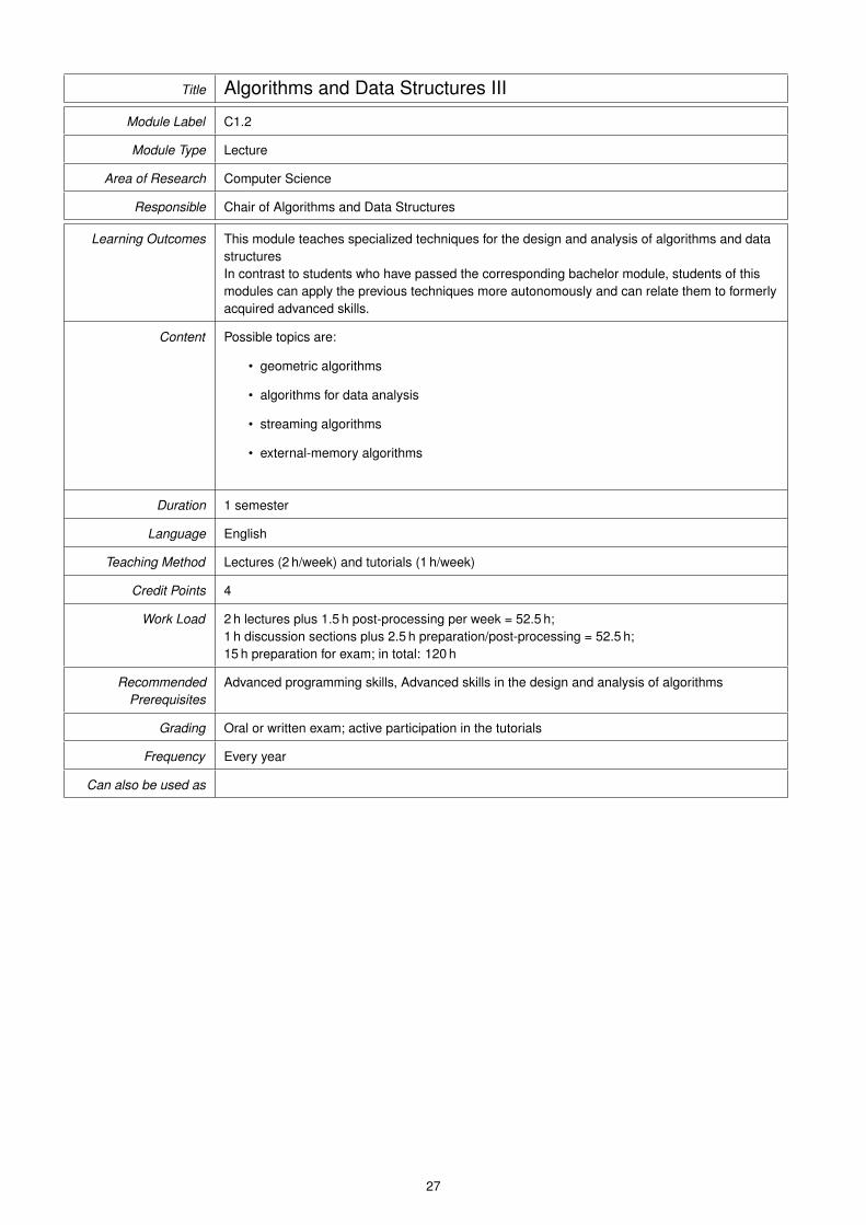
Title Algorithms and Data Structures III

Module Label C1.2

Module Type Lecture


Responsible Chair of Algorithms and Data Structures

Learning Outcomes This module teaches specialized techniques for the design and analysis of algorithms and datastructuresIn contrast to students who have passed the corresponding bachelor module, students of thismodules can apply the previous techniques more autonomously and can relate them to formerlyacquired advanced skills.

Content Possible topics are:

• geometric algorithms

• algorithms for data analysis

• streaming algorithms

• external-memory algorithms

Duration 1 semester

Language English


Credit Points 4



Advanced programming skills, Advanced skills in the design and analysis of algorithms



Can also be used as

27

Title Parallel and Distributed Systems I

Module Label C1.3

Module Type Lecture


Responsible Chair of Parallel and Distributed Systems

Learning Outcomes The goal of this course is to impart to the students basic techniques in parallel and distributedprogramming. By that, special methodical competences are acquired: By understanding basicproblems such as load balancing and scalability and by learning synchronization andcommunication techniques, the students are enabled to design and, with the help ofcommunication and thread libraries, to transform parallel algorithms into efficient parallel anddistributed programs. By that, both shared and distributed address spaces are acquired.In contrast to students who have passed the corresponding bachelor module, students of thismodules can apply the previous techniques more autonomously and can relate them to formerlyacquired advanced skills.

Content • Architecture and interconnection networks for parallel systems

• Performance analysis and scalability of parallel programs

• Programming and synchronization techniques for shared address space withmulti-threading

• Coordination of parallel and distributed programs

• Application of programming techniques to complex examples from different areas

• Programming techniques for distributed address spaces and message-passing

Duration 1 semester

Language German


Credit Points 4

Work Load 120 h in total (45 h presence, 60 h preparation/post-processing, 15 h preparation for exam)


Grading Written exam; For the admission to the written exam a vivid participation in the exercises isrequired.

Frequency Every year in winter term

Can also be used as

28

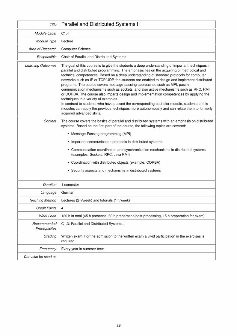
Title Parallel and Distributed Systems II

Module Label C1.4

Module Type Lecture



Learning Outcomes The goal of this course is to give the students a deep understanding of important techniques inparallel and distributed programming. The emphasis lies on the acquiring of methodical andtechnical competences. Based on a deep understanding of standard protocols for computernetworks such as IP or TCP/UDP, the students are enabled to design and implement distributedprograms. The course covers message-passing approaches such as MPI, passivcommunication mechanisms such as sockets, and also active mechanisms such as RPC, RMI,or CORBA. The course also imparts design and implementation competences by applying thetechniques to a variety of examples.In contrast to students who have passed the corresponding bachelor module, students of thismodules can apply the previous techniques more autonomously and can relate them to formerlyacquired advanced skills.

Content The course covers the basics of parallel and distributed systems with an emphasis on distributedsystems. Based on the first part of the course, the following topics are covered:

• Message-Passing programming (MPI)

• Important communication protocols in distributed systems

• Communication coordination and synchronization mechanisms in distributed systems(examples: Sockets, RPC, Java RMI)

• Coordination with distributed objects (example: CORBA)

• Security aspects and mechanisms in distributed systems

Duration 1 semester

Language German


Credit Points 4



C1.3: Parallel and Distributed Systems I


Frequency Every year in summer term

Can also be used as

29

Title High-Performance Computing

Module Label C1.5

Module Type Lecture



Learning Outcomes The goal of this course is to give the students a deep understanding of important techniques ofprogram analysis and program transformation. The emphasis lies on the acquiring of analyticaland technological competences: the students are enabled to analyse arbitrary programs byapplying the techniques of data and control dependency analysis and to perform optimizingprogram transformation based on these analysis techniques. Examples are the vectorizationand parallelization of program parts or optimization towards a given memory hierarchy.Methodical and algorithmis competences are acquired by learning scheduling and loadbalancing algorithms and the underlying principles.In contrast to students who have passed the corresponding bachelor module, students of thismodules can apply the previous techniques more autonomously and can relate them to formerlyacquired advanced skills.

Content The following topics are covered:

• Overview of current processor architectures and interconnection technologies

• Control flow and data flow analysis, data flow equations and solution methods for dataflow equations, optimizing transformations

• Data dependency analysis, loop dependencies, data dependence equations and solutionmethods for them

• Program transformations for vectorization, parallelization and cache optimization

• Methods for scheduling and load balancing for instructions, loops, and tasks

• OpenMP programming

• Register allocation and program tranformations for reducing the register need of programs

• CPU programming with CUDA

Duration 1 semester

Language English


Credit Points 8

Work Load 240 h in total (90 h presence, 150 h preparation/post-processing with processing of worksheets)


C1.3: Parallel and Distributed Systems I



Can also be used as

30

Title Parallel Algorithms

Module Label C1.6

Module Type Lecture



Learning Outcomes Students acquire in-depth knowledge about selected parallel algorithms from different fields ofapplication. In particular, in connection with exercises, students gain analytical andmethodological expertise, which empowers them to understand, implement, analyse, and designparallel algorithms.In contrast to students who have passed the corresponding bachelor module, students of thismodules can apply the previous techniques more autonomously and can relate them to formerlyacquired advanced skills.

Content Selected parallel algorithms are presented. The range extends from basic, widespreadalgorithms (e.g., sorting) to complex algorithms from specific fields of application (e.g., computergraphics). Emphasis is put on algorithms from the field of scientific computing. The exercisescover theoretical problems as well as practical programming experience.

Duration 1 semester

Language English


Credit Points 4



Algorithms and Data Structures I, C1.3: Parallel and Distributed Systems I



Can also be used as

31

Title Programming and Data Analysis in Python

Module Label C1.7

Module Type Lecture


Responsible Chair of Serious Games

Learning Outcomes Students learn to quickly prototype and implement numerical programs in Python. They learnPython as a programming language and a scientific computing environment. They acquireknowledge of the basic programming language, as well as of important libraries for scientificcomputing, such as NumPy, SciPy, Matplotlib, Pandas, and TensorFlow/Keras. They developpractical and applied skills in exploratory computing, rapid prototyping, and implementation ofnumerical methods. In contrast to other environments, the Python scientific computingenvironment is open source, widely used, optimized for programmer productivity, and benefitsfrom a large community and library ecosystem.

Content The Python programming language: Programming philosophy in Python, data types, controlstructures, functions, object-oriented programming, debugging. Algorithms: Basic algorithms(e.g., searching and sorting), bisection, recursion, dynamic programming, Newton’s method.Matrix methods: Linear Algebra with NumPy, matrix factorizations, eigenvectors and values,diagonalization, SVD, least squares and pseudoinverse. Data analysis: Pandas, clustering,plotting. Neural networks and deep learning.

Duration 1 semester

Language English


Credit Points 4



None

Grading Oral or written exam (85%), exercises (15%)

Frequency Every year in winter term

Can also be used as

32

3.2 Module C2: Practical Course on Parallel Numerical Methods

Title Parallel Numerical Methods

Module Label C2

Module Type Pratical course

Area of Research Computer Science, Scientific Computing

Responsible Chairs of Parallel and Distributed Systems, Scientific Computing

Learning Outcomes • Implementation of parallel algorithms:select suitable efficient numerical methodschoose data structures that are suitable for the respective problemimplement the numerical methods on a parallel computer using standard libraries

• Presentation and discussion:choose and master suitable presentation techniquesspeak freely about a subject and illustrate important structures instructivelyanswer spontaneous questions from the audience in a reliable manner

Content In this practical course, students implement manageable numerical problems (such as Gaussianelimination, finite element discretization of 2d Laplacian, etc.) on parallel computers using theprogramming language C/C++ and standard software libraries (LAPACK/BLAS, OpenMP,OpenMPI). The resulting parallel efficiency is observed depending on the chosenimplementation (naive or advanced such as Schwarz methods).

Duration 1 semester

Language English

Teaching Method Practical course (2 weeks)

Credit Points 2

Work Load 50 h practical course; 10 h preparation for exam; in total: 60 h


A1: Numerical Methods for Differential Equations, C1.3: Parallel and Distributed Systems I,D1.1: Efficient Treatment of Non-local Operators

Grading Implementation and presentation of approaches; active participation and discussion

Frequency Every year at the end of the winter term

Can also be used as

33

4 Module Section D: Scientific Computing

4.1 Elective Modules D1: Complexity Reduction

Title Efficient Treatment of Non-local Operators

Module Label D1.1

Module Type Lecture



Learning Outcomes • Understanding the way numerical algorithms for the solution of partial differential andintegral equations work

• Understanding that non-local operators may contain redundancies which can be used toreduce their asymptotic complexity

• Ability to choose a suitable algorithm for a given class of partial differential and integralequations

• Ability to implement the algorithms discussed in the lecture in a higher programminglanguage on a parallel computer

Content State-of-the-art linear complexity treatment of partial differential and integral operators andparallelization techniques:

• fast multipole methods for the efficient treatment of multi-source potentials (one of theTOP10 algorithms from the 20th century)

• hierarchical matrices (for the treatment of non-local operators with linear complexity)

• Schwarz methods (additive and multiplicative)

• BPX preconditioner

• Domain decomposition (overlapping and non-overlapping), BPS and Neumann-Neumannpreconditioners, FETI

Duration 1 semester

Language English


Credit Points 8






34

Title Fast Methods for Differential and Integral Equations

Module Label D1.2

Module Type Lecture



Learning Outcomes • Understanding the way numerical algorithms for the solution of partial differential andintegral equations work

• Detection of suitable structures which can be exploited for the complexity reduction ofsolution operators of elliptic boundary value problems

• Ability to choose a suitable algorithm for a given class of partial differential or integralequations

• Ability to implement the algorithms discussed in the lecture in a higher programminglanguage

Content Numerical analysis of optimal complexity solvers for the treatment of boundary value problems;efficient treatment of parameter-dependent problems:

• subspace correction methods

• hierarchical bases and BPX preconditioners

• geometric and algebraic multigrid methods (convergence and implementation aspects)

• reduced bases methods

• analysis of hierarchical matrices

Duration 1 semester

Language English


Credit Points 8







35

Title Efficient Numerical Treatment of Multiscale Problems

Module Label D1.3

Module Type Lecture



Learning Outcomes • Understanding of key mechanisms and challenges in scale interaction for the PDE-basedequations and systems in scientific and technical problems

• Ability to identify and apply a suitable modeling and/or numerical technique for a widerange of multiscale problems

• Ability to implement the mathematical methods and numerical algorithms introduced in thecourse using a programming language

Content Modeling approaches:

• asymptotic analysis

• homogenization

• Reynolds-averaged Navier-Stokes (RANS), large eddy simulation (LES)

Numerical methods:

• multiscale finite element method (MsFEM)

• variational multiscale method

• wavelet-based discretizations

• reduced-basis methods

• heterogeneous multiscale methods (HMM)

Duration 1 semester

Language English


Credit Points 8







36

Title Numerical Methods for Uncertainty Quantification

Module Label D1.4

Module Type Lecture



Learning Outcomes

Content This is a cutting-edge area of Scientific Computing. In addition to Monte Carlo methods,stochatic collocation, polyonomial chaos expansions, stochastic Galerkin methods, theKarhunen-Loeve expansion, model order reduction, and multilevel quadrature recentdevelopments in this area are to be discussed.

Duration 1 semester

Language English


Credit Points 4

Work Load 2 h lectures plus 3 h post-processing per week = 52,5 h;1 h discussion sections plus 2,5 h preparation/post-processing = 52,5 h;15 h preparation for exam; in total: 120 h






37

Title High-dimensional Approximation

Module Label D1.5

Module Type Lecture


Responsible Chairs of Applied and Numerical Analysis, Scientific Computing


• understand the curse of dimensionality

• know several concepts to reduce the complexity in high-dimensional problems

• be able to apply such concepts to typical examples from finance, physics and engineering

Content • Introduction to problems from finance, physics and engineering leading tohigh-dimensional partial differential equations, such as Black-Scholes and Fokker-Planck

• Modern concepts for high-dimensional problems including tensor product methods,sparse grids, kernel-based methods, Monte-Carlo and Quasi-Monte-Carlo methods

• Error and stability analysis of such methods

• Efficient algorithms for and implementations of such methods

Duration 1 semester

Language English


Credit Points 4

Work Load 2 h lectures plus 1,5 h post-processing per week = 52,5 h;1 h discussion sections plus 2,5 h preparation/post-processing = 52,5 h;15 h preparation for exam; in total: 120 h






38

Title Data Analytics

Module Label D1.6

Module Type Lecture


Responsible Chair for Databases and Information Systems

Learning Outcomes Conceptual foundation of development of large databases (Big Data) and information systemswith focus on modeling. Deepening of proficiency in databases in the context of large andcomplex database and web applications; imparting of interdisciplinary, analytical competencesfor reconstructing and modeling complex applications (mostly stemming from the applicationfields); technological competence for selecting and integrating heterogeneous modeling andimplementation concepts for the design and realization of data and process based applications.Deepening of proficiency in the fields of data analytics. Realization of complex architectures inthe application fields Bio Informatics, Environmental Informatics and Engineer Informatics will bediscussed in all courses.In contrast to students who have passed the corresponding bachelor module, students of thismodules can apply the previous techniques more autonomously and can relate them to formerlyacquired advanced skills.

Content first semester: Data Warehousing, Data Miningsecond semester: Data Visualisation, Machine Learning, Ontologies, NoSQL, DistributedComputing Concepts (MapReduce, Hadoop, etc.)


Language English


Credit Points 8



Datenbanken und Informationssysteme I


Frequency Every year during winter and summer term

Can also be used as

39

Title Complexity Reduction in Control

Module Label D1.7

Module Type Lecture



Learning Outcomes • Understanding why many numerical approaches to control problems suffer from the curseof dimensionality

• Recognition of redundancies, such as the turnpike property in optimal control problems,and their use for complexity reduction

• Knowledge about state-of-the-art model order reduction methods for linear and nonlinearcontrol systems and how they rely on the particular input-output-structure

• Ability to identify suitable techniques for particular applications

Content • State-of-the-art techniques for the reduction of complexity in control problems, as forinstance

– Model predictive control and its use as a complexity reduction technique

– Sparse grid and parallel computing approaches for Hamilton-Jacobi-Bellmanequations

– Model order reduction methods for control systems, such as balanced truncation orproper orthogonal decomposition

• Implementation of selected algorithms in the tutorials

Duration 1 semester

Language English


Credit Points 4



A2.4: Mathematical Control Theory, A1: Numerical Methods for Differential Equations




40

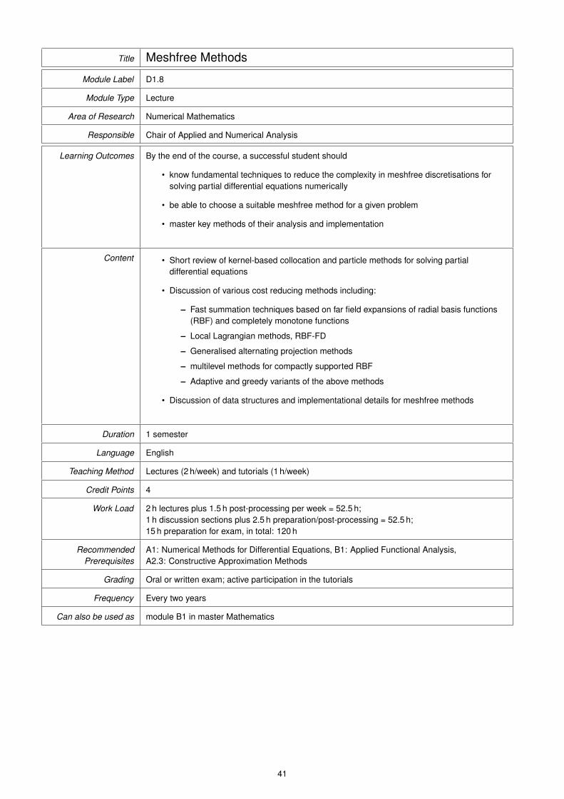
Title Meshfree Methods

Module Label D1.8

Module Type Lecture


Responsible Chair of Applied and Numerical Analysis


• know fundamental techniques to reduce the complexity in meshfree discretisations forsolving partial differential equations numerically

• be able to choose a suitable meshfree method for a given problem

• master key methods of their analysis and implementation

Content • Short review of kernel-based collocation and particle methods for solving partialdifferential equations

• Discussion of various cost reducing methods including:

– Fast summation techniques based on far field expansions of radial basis functions(RBF) and completely monotone functions

– Local Lagrangian methods, RBF-FD

– Generalised alternating projection methods

– multilevel methods for compactly supported RBF

– Adaptive and greedy variants of the above methods

• Discussion of data structures and implementational details for meshfree methods

Duration 1 semester

Language English


Credit Points 4

Work Load 2 h lectures plus 1.5 h post-processing per week = 52.5 h;1 h discussion sections plus 2.5 h preparation/post-processing = 52.5 h;15 h preparation for exam, in total: 120 h


A1: Numerical Methods for Differential Equations, B1: Applied Functional Analysis,A2.3: Constructive Approximation Methods




41

Title Boundary Element Methods

Module Label D1.9

Module Type Lecture



Learning Outcomes Exterior boundary value problems are difficult to treat via finite element discretizations due to theunboundedness of the computational domain. This lecture presents a different approach bywhich the boundary value problem is reformulated as an integral equation on the boundary. Inparticular, this offers the advantage that only a lower-dimensional set has to be discretized. As aconsequence, the resulting linear systems are significantly smaller but fully populated in general.The latter difficulty can be treated by local low-rank approximation.

By the end of the course, a successful student should

• know fundamental techniques to reduce suitable boundary value problems to boundaryintegral equations

• master key methods of the analysis and implementation of boundary integral methods

• be able to reduce the complexity of suitable discrete non-local operators

Content • Sobolev spaces on manifolds

• fundamental solutions of partial differential operators

• boundary integral operators and their properties

• boundary integral equations and their finite element discretization

• generating the matrix coefficients

• fast boundary element methods

• applications: potential equation, linear elasticity, Stokes equations

Duration 1 semester

Language English


Credit Points 4

Work Load 2 h lectures plus 1.5 h post-processing per week = 52.5 h;1 h discussion sections plus 2.5 h preparation/post-processing = 52.5 h;15 h preparation for exam, in total: 120 h






42

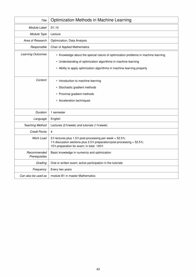
Title Optimization Methods in Machine Learning

Module Label D1.10

Module Type Lecture

Area of Research Optimization, Data Analysis


Learning Outcomes • Knowledge about the special nature of optimization problems in machine learning

• Understanding of optimization algorithms in machine learning

• Ability to apply optimization algorithms in machine learning properly

Content • Introduction to machine learning

• Stochastic gradient methods

• Proximal gradient methods

• Acceleration techniques

Duration 1 semester

Language English


Credit Points 4



Basic knowledge in numerics and optimization




43

4.2 Module D2: Special Skills in Scientific Computing

Title Special Skills in Scientific Computing

Module Label D2

Module Type Lecture

Area of Research Numerical Mathematics, Scientific Computing

Responsible Chairs of Applied and Numerical Analysis, Applied Mathematics, Scientific Computing

Learning Outcomes The goal of this module is to provide students with special skills in the areas of NumericalMathematics and Scientific Computing, relevant for current research activities.

Content An active field of mathematical research, in which specialized techniques are applied or in whichknown techniques from different areas are combined in an original way. Examples are:

1. Fractional order differential operators

2. Optimization of nonsmooth problems

3. Advanced topics of optimization with partial differential equations

4. mathematical control theory for infinite-dimensional systems

Duration 1 semester

Language English


Credit Points 4



Advanced status of study



Can also be used as

44

5 Module Section E: Soft Skills

Title Soft Skills

Module Label E

Module Type Seminar

Area of Research

Responsible Programme coordinator

Learning Outcomes Key skills for personal development

Content Participation in seminars devoted to presentation skills, data processing, literature research,handling of foreign-language literature, teamwork, etc.; for instance, the seminars academicwriting, embodied communication, and time- and self-management are offered regularly by theElite Network of Bavaria; the programme coordinator and your mentor will give individualrecommendations

Duration 1 semester

Language English

Teaching Method Participation in seminars

Credit Points 2

Work Load In total 60 h of seminars, i.e. 3–4 seminars


None

Grading Proof of attendance

Frequency

Can also be used as

45

6 Module Section F: Master’s Thesis

Title Master’s Thesis

Module Label F

Module Type Thesis

Area of Research all areas

Responsible Programme coordinator

Learning Outcomes Ability to prepare a scientific work (larger than a bachelor’s thesis)

Content Scientific work in the area of Scientific Computing that should have a connection withapplication-driven questions and with the focus of this master’s programme. In particular,interdisciplinary problems should be treated.


Language English or German

Teaching Method

Credit Points 30

Work Load 900 h (editing time: at most 10 months)


Grading Written thesis

Frequency

Can also be used as

46

7 Recommended Curriculum

The following recommended curriculum assumes that the studies start in winter term.

a) Full-time study

47

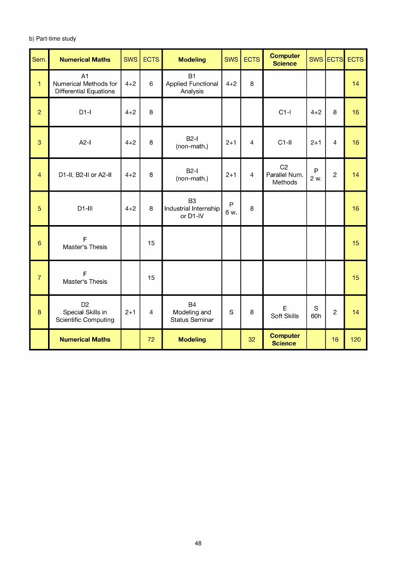
b) Part-time study

48

The following recommended curriculum assumes that the studies start in summer term.

a) Full-time study

49

b) Part-time study

50

book of modules for the elite master's programme

Documents