Boosting-Based Multimodal Speaker Detection

for Distributed Meeting VideosCha Zhang, Pei Yin, Yong Rui, Ross Cutler, Paul Viola, Xinding Sun, Nelson Pinto and

Zhengyou Zhang

Abstract

Identifying the active speaker in a video of a distributed meeting can be very helpful for remote participants to

understand the dynamics of the meeting. A straightforward application of such analysis is to stream a high resolution

video of the speaker to the remote participants. In this paper, we present the challenges we met while designing

a speaker detector for the Microsoft RoundTable distributed meeting device, and propose a novel boosting-based

multimodal speaker detection (BMSD) algorithm. Instead of separately performing sound source localization (SSL)

and multi-person detection (MPD) and subsequently fusing their individual results, the proposed algorithm fuses

audio and visual information at feature level by using boosting to select features from a combined pool of both audio

and visual features simultaneously. The result is a very accurate speaker detector with extremely high efficiency. In

experiments that includes hundreds of real-world meetings, the proposed BMSD algorithm reduces the error rate of

SSL-only approach by 24.6%, and the SSL and MPD fusion approach by 20.9%. To the best of our knowledge, this

is the first real-time multimodal speaker detection algorithm that is deployed in commercial products.

Index Terms

speaker detection, boosting, audio visual fusion.

C. Zhang, Y. Rui, P. Viola and Z. Zhang are with Microsoft Research, One Microsoft Way, Redmond, USA.

P. Yin is with College of Computing, Georgia Institute of Technology, Atlanta, Georgia, USA.

R. Cutler, X. Sun and N. Pinto are with Microsoft Corp., One Microsoft Way, Redmond, USA.

August 7, 2008 DRAFT

IEEE TRANS. ON MULTIMEDIA, VOL. X, NO. X, XXX 2008 1

Boosting-Based Multimodal Speaker Detection

for Distributed Meeting Videos

I. INTRODUCTION

As globalization continues to spread throughout the world economy, it is increasingly common to find projects

where team members reside in different time zones. To provide a means for distributed groups to work together on

shared problems, there has been an increasing interest in building special purpose devices and even “smart rooms”

to support distributed meetings [1], [2], [3], [4]. These devices often contain multiple microphones and cameras.

An example device called RoundTable is shown in Fig. 1(a). It has a six-element circular microphone array at

the base, and five video cameras at the top. The captured videos are stitched into a 360 degree panorama, which

gives a global view of the meeting room. The RoundTable device enables remote group members to hear and view

the meeting live online. In addition, the meetings can be recorded and archived, allowing people to browse them

afterward.

One of the most desired features in such distributed meeting systems is to provide remote users with a close-up

of the current speaker which automatically tracks as a new participant begins to speak [2], [3], [4]. The speaker

detection problem, however, is non-trivial. Two video frames captured by our RoundTable device are shown in

Fig. 1(b). During the development of our RoundTable device, we faced a number of challenges:

• People do not always look at the camera, in particular when they are presenting on a white board, or working

on their own laptops.

• There can be many people in a meeting, hence it is very easy for the speaker detector to get confused.

• The color calibration in real conference rooms is very challenging. Mixed lighting across the room makes it

very difficult to properly white balance across the panorama images. Face detection based on skin color is

very unreliable in such environments.

• To make the RoundTable device stand-alone, we have to implement the speaker detection module on a DSP

chip with the budget of 100 million instructions per second (MIPS). Hence the algorithm must be extremely

efficient. Our initial goal is to detect speaker at the speed of 1 frame per second (FPS) on the DSP.

• While the RoundTable device captures very high resolution images, the resolution of the images used for

speaker detection is low due to the memory and bandwidth constraints of the DSP chip. For people sitting at

the far end of the table, the head size is no more than 10× 10 pixels, which is beyond the capability of most

modern face detectors [5].

In existing distributed meeting systems, the two most popular speaker detection approaches are through sound

source localization (SSL) [6], [7] and SSL combined with face detection using decision level fusion (DLF) [3], [4].

However, they both have difficulties in practice. The success of SSL heavily depends on the levels of reverberation

August 7, 2008 DRAFT

IEEE TRANS. ON MULTIMEDIA, VOL. X, NO. X, XXX 2008 2

(b)(a)

Fig. 1. RoundTable and its captured images. (a) The RoundTable device. (b) Captured images.

noise (e.g., a wall or whiteboard can act as an acoustic mirror) and ambient noise (e.g., computer fans), which are

often high in many meeting rooms. If a face detector is available, decision level fusion can certainly help improve

the final detection performance. However, building a reliable face detector in the above mentioned environment is

itself a very challenging task.

In this paper, we propose a novel boosting-based multimodal speaker detection (BMSD) algorithm, which attempts

to address most of the challenges listed above. The algorithm does not try to locate human faces, but rather heads

and upper bodies. By integrating audio and visual multimodal information into a single boosting framework at the

feature level, it explicitly learns the difference between speakers and non-speakers. Specifically, we use the output

of an SSL algorithm to compute audio related features for windows in the video frame. These features are then

placed in the same pool as the appearance and motion visual features computed on the gray scale video frames,

and selected by the boosting algorithm automatically. The BMSD algorithm reduces the error rate of the SSL-only

solution by 24.6% in our experiments, and the SSL and person detection DLF approach by 20.9%. The BMSD

algorithm is super-efficient. It achieves the above performance with merely 60 SSL and Haar basis image features.

Lastly, BMSD does not require high frame rate video analysis or tight AV synchronization, which is ideal for

our application. The proposed BMSD algorithm has been integrated with the RoundTable device and shipped to

thousands of customers in the summer of 2007.

The paper is organized as follows. Related work is discussed in Section II. A new maximum likelihood based

SSL algorithm is briefly presented in Section III. The BMSD algorithm is described in Section IV. Experimental

results and conclusions are given in Section V and VI, respectively.

II. RELATED WORK

Audio visual information fusion has been a popular approach for many research topics including speech recog-

nition [8], [9], video segmentation and retrieval [10], event detection [11], [12], speaker change detection [13],

speaker detection [14], [15], [16], [17] and tracking [18], [19], etc. In the following paragraphs we describe briefly

a few approaches that are closely related to this paper.

Audio visual synchrony is one of the most popular mechanisms to perform speaker detection. Explicitly or

implicitly, many approaches measure the mutual information between audio visual signals and search for regions

August 7, 2008 DRAFT

IEEE TRANS. ON MULTIMEDIA, VOL. X, NO. X, XXX 2008 3

of high correlation and tag them as likely to contain the speaker. Representative works include Hershey and

Movellan [16], Nock et al. [20], Besson and Kunt [14], and Fisher et al. [15]. Cutler and Davis [21] instead

learned the audio visual correlation using a time-delayed neural network (TDNN). Approaches in this category

often need just a single microphone, and rely on the synchrony only to identify the speaker. Most of them require

a good frontal face to work well.

Another popular approach is to build graphical models for the observed audio visual data, and infer the speaker

location probabilistically. Pavlovic et al. [17] proposed to use dynamic Bayesian networks (DBN) to combine

multiple sensors/detectors and decide whether a speaker is present in front of a smart kiosk. Beal et al. [22] built

a probabilistic generative model to describe the observed data directly using an EM algorithm and estimated the

object location through Bayesian inference. Brand et al. [11] used coupled hidden Markov models to model the

relationship between audio visual signals and classify human gestures. Graphical models are a natural way to solve

multimodal problems and are often intuitive to construct. However, their inference stage can be time-consuming

and would not fit into our tight computation budget.

Audio visual fusion has also been applied for speaker tracking, in particular those based on particle filtering [18],

[19], [23], [24]. In the measurement stage, audio likelihood and video likelihood are both computed for each sample

to derive its new weight. It is possible to use these likelihoods as measures for speaker detection, though such an

approach can be very expensive if all the possible candidates in the frame need to be scanned.

In real-world applications, the two most popular speaker detection approaches are still SSL-only and SSL

combined with face detection for decision level fusion [2], [3], [4]. For instance, the iPower 900 teleconferencing

system from Polycom uses an SSL-only solution for speaker detection [6]. Kapralos et al. [3] used a skin color

based face detector to find all the potential faces, and detect speech along the directions of these faces. Yoshimi

and Pingali [4] took the audio localization results and used a face detector to search for nearby faces in the image.

Busso et al. [1] adopted Gaussian mixture models to model the speaker locations, and fused the audio and visual

results probabilistically with temporal filtering.

As mentioned earlier, speaker detection based on SSL-only is sensitive to reverberation and ambient noises.

The DLF approach, on the other hand, has two major drawbacks in speaker detection. First, when SSL and face

detection operate separately, the correlation between audio and video, either at high frame rate or low frame rate,

is lost. Second, a full-fledged face detector can be unnecessarily slow, because many regions in the video can be

skipped if their SSL confidence is too low. Limiting the search range of face detection near SSL peaks, however, is

difficult because it is hard to find a universal SSL threshold for all conference rooms. Moreover, this can introduce

bias towards the decision made by SSL. The proposed algorithm uses a boosted classifier to perform feature level

fusion of information in order to minimize computation time and maximize robustness. We will show the superior

performance of BMSD by comparing it with the SSL-only and DLF approaches in Section V.

August 7, 2008 DRAFT

IEEE TRANS. ON MULTIMEDIA, VOL. X, NO. X, XXX 2008 4

III. SOUND SOURCE LOCALIZATION

Because the panoramic video available for speaker detection is at very low resolution, it is very challenging even

for humans to tell who is the active speaker. Consequently, we first investigated the idea of building a better SSL

algorithm that is less sensitive to reverberation or ambient noises. We developed a novel maximum likelihood (ML)

based sound source localization algorithm that is both efficient and robust to reverberation and noises [25]. In the

proposed BMSD algorithm, audio related features are extracted from the output of the ML based SSL algorithm

instead of the original audio signal. For the completeness of this paper, we provide a brief review of the ML based

SSL algorithm in this section, and refer the readers to [25] for more details.

Consider an array of P microphones (In the case of RoundTable, there are a total of 6 directional microphones

on the base of the device). Given a source signal s(t), the signals received at these microphones can be modeled

as [26]:

xi(t) = αis(t− τi) + hi(t)⊗ s(t) + ni(t), (1)

where i = 1, · · · , P is the index of the microphones, τi is the time of propagation from the source location to

the ith microphone; αi is a gain factor that includes the propagation energy decay of the signal, the gain of the

corresponding microphone, the directionality of the source and the microphone, etc; ni(t) is the noise sensed by

the ith microphone; hi(t)⊗ s(t) represents the convolution between the environmental response function hi(t) and

the source signal, often referred as the reverberation.

In the frequency domain, the equivalent form of the above model is:

Xi(ω) = αi(ω)S(ω)e−jωτi + Hi(ω)S(ω) + Ni(ω), (2)

where we allow the αi to vary with frequency. In a vector form:

X(ω) = S(ω)G(ω) + S(ω)H(ω) + N(ω), (3)

where

X(ω) = [X1(ω), · · · , XP (ω)]T ,

G(ω) = [α1(ω)e−jωτ1 , · · · , αP (ω)e−jωτP ]T ,

H(ω) = [H1(ω), · · · ,HP (ω)]T ,

N(ω) = [N1(ω), · · · , NP (ω)]T .

Our ML based SSL algorithm makes the assumption that the combined total noise,

Nc(ω) = S(ω)H(ω) + N(ω), (4)

follows a zero-mean, independent between frequencies, joint Gaussian distribution, i.e.,

p(Nc(ω)) = ρ exp{− 1

2[Nc(ω)]HQ−1(ω)Nc(ω)

}, (5)

August 7, 2008 DRAFT

IEEE TRANS. ON MULTIMEDIA, VOL. X, NO. X, XXX 2008 5

where ρ is a constant; superscript H represents Hermitian transpose, Q(ω) is the covariance matrix of the combined

noise and can be estimated from the received audio signals.

The likelihood of the received signals can be written as:

p(X|S,G,Q) =∏ω

p(X(ω)|S(ω),G(ω),Q(ω)), (6)

where

p(X(ω)|S(ω),G(ω),Q(ω)) = ρ exp{− J(ω)/2

}, (7)

J(ω) = [X(ω)− S(ω)G(ω)]HQ−1(ω)[X(ω)− S(ω)G(ω)]. (8)

The goal of the proposed sound source localization is thus to maximize the above likelihood, given the observations

X(ω), gain matrix G(ω) and noise covariance matrix Q(ω). Note the gain matrix G(ω) requires information about

where the sound source comes from, hence the optimization is usually solved through hypothesis testing. That is,

hypotheses are made about the source source location, which can be used to compute the corresponding G(ω). The

likelihood are then measured. The hypothesis that results in the highest likelihood is determined to be the output

of the SSL algorithm.

We showed that the solution to such a ML problem is to use hypothesis testing to measure the maximum value

of

L =∫

ω

[GH(ω)Q−1(ω)X(ω)]HGH(ω)Q−1(ω)X(ω)GH(ω)Q−1(ω)G(ω)

dω. (9)

Under certain simplified conditions, the above criterion can be computed efficiently. More specifically, one may

hypothesize the source locations, measure and maximize the following objective function:

J =∫

ω

∣∣∣ ∑Pi=1

Xi(ω)ejωτi

κi(ω)

√|Xi(ω)|2 − E{|Ni(ω)|2}

∣∣∣2

∑Pi=1

1κi(ω) (|Xi(ω)|2 − E{|Ni(ω)|2})

dω, (10)

where

κi(ω) = γ|Xi(ω)|2 + (1− γ)E{|Ni(ω)|2}, (11)

and γ is a parameter modeling the severity of room reverberation. Interested readers are referred to [25] for more

details about the assumptions and derivations.

The ML based SSL algorithm significantly improved the localization accuracy over traditional SSL algorithms

such as SRP-PHAT [27], in particular under very noisy environments. However, it may still be deceived by heavy

reverberation and points to directions where no people are there. In the next section, we present the boosting-based

multimodal speaker detection algorithm that aims to use visual information to further improve the speaker detection

performance.

IV. BOOSTING-BASED MULTIMODAL SPEAKER DETECTION

Our speaker detection algorithm adopts the popular boosting algorithm [28], [29] to learn the difference between

speakers and non-speakers. It computes both audio and visual features, and places them in a common feature pool

August 7, 2008 DRAFT

IEEE TRANS. ON MULTIMEDIA, VOL. X, NO. X, XXX 2008 6

(b)

(c)

(d)

(e)

(a)

A B

Fig. 2. Motion filtering in BMSD. (a) Video frame at t− 1. (b) Video frame at t. (c) Difference image between (a) and (b). (d) Three frame

difference image. (e) Running average of the three frame difference image.

for the boosting algorithm to select. This has a number of advantages. First, the boosting algorithm explicitly learns

the difference between a speaker and a non-speaker, thus it targets the speaker detection problem more directly.

Second, the final classifier can contain both audio and visual features, which implicitly explores the correlation

between the audio and visual information if they coexist after the feature selection. Third, thanks to the cascade

pruning mechanism introduced in [5], audio features selected early in the learning process will help eliminate many

non-speaker windows, which greatly improves the detection speed. Finally, since all the audio visual features are

in the same pool, there is no bias toward either modality.

In the following subsections we first introduce the visual and audio features, then present the boosting learning

algorithm. We also briefly discuss the SSL-only and SSL and multi-person detector (MPD) DLF algorithms, which

will be used in Section V to compare against BMSD.

A. Visual Features

Appearance and motion are two important visual cues to tell a person from the background [30]. The appearance

cue is generally derived from the original video frame, hence we focus on the motion cue in this section.

The simplest motion filter is to compute the frame difference between two subsequent frames [30]. When applied

to our testing sequences, we find two major problems, demonstrated in Fig. 2. Fig. 2(a) and (b) are two subsequent

August 7, 2008 DRAFT

IEEE TRANS. ON MULTIMEDIA, VOL. X, NO. X, XXX 2008 7

Fig. 3. Example rectangle features shown relative to the enclosing detection window. Left: 1-rectangle feature; right: 2-rectangle feature.

frames captured in one of the recorded meetings. Person A was walking toward the whiteboard to give a presentation.

Because of the low frame rate the detector is running at, the difference image (c) has two big blobs for person

A. Experiments show that the boosting algorithm often selects motion features among its top features, and such

ghost blobs tend to cause false positives. Person B in the scene shows another problem. In a regular meeting, often

someone in the room stays still for a few seconds, hence the frame difference of person B is very small. This tends

to cause false negatives.

To address the first problem, we use a simple three frame difference mechanism to derive the motion pattern.

Let It be the input image at time t, we compute:

Mt = min(|It − It−1|, |It − It−2|

). (12)

As shown in Fig. 2(d), Eq. (12) detects a motion region only when the current frame has large difference with the

previous two frames, and can thus effectively remove the ghost blobs in Fig. 2(c). Note three frame difference was

used in background modeling before [31].

We add another frame as Fig. 2(e), which is the running average of the three frame difference images:

Rt = αMt + (1− α)Rt−1. (13)

The running difference image accumulates the motion in the history, and captures the long-term motion of people

in the room. It can be seen that even though person B moved very slightly in this particular frame, the running

difference image is still able to capture his body clearly.

Despite their simplicity, the two added images reduce the detection error significantly. We also experimented by

replacing Eq. (12) with a background subtraction module such as the one in [32]. Only marginal improvement was

observed with a relatively high computational cost (for our application).

Given the three frames It, Mt and Rt, we use two kinds of simple visual features to train the classifier, as shown

in Fig. 3. Similar to [5], these features are computed for each detection window of the video frame. Note each

detection window will cover the same location on all three images. The 1-rectangle feature on the left of Fig. 3 is

computed on the difference image and running difference image only. Single rectangle features allow the classifier

to learn a data dependent and location dependent difference threshold. The 2-rectangle feature on the right is applied

to all three images. This arrangement is to guarantee that all the features have zero-mean, so that they are less

August 7, 2008 DRAFT

IEEE TRANS. ON MULTIMEDIA, VOL. X, NO. X, XXX 2008 8

Rectangle to classify(a)

(b) u0 u1

Fig. 4. Compute SSL features for BMSD. (a) Original image. (b) SSL image. Bright intensity represents high likelihood. Note the peak of

the SSL image does not correspond to the actual speaker (the right-most person), indicating a failure for the SSL-only solution.

sensitive to lighting variations. For our particular application, we found adding more features such as 3-rectangle

or 4-rectangle features gave very limited improvements on the classifier performance.

B. Audio Features

We extract audio features based on the output of the hypothesis testing process during SSL. Note the microphone

array on the RoundTable has a circular geometry. Hence the SSL can only provide reliable 1D azimuth of the

sound source location through hypothesis testing. We obtain a 1D array of numbers between 0 and 1 following

Eq. (9), denoted as La(θ), θ = 0, α, · · · , 360−α. The hypothesis testing is done for every α degrees. In the current

implementation, α = 4 gives good results. We perform SSL at 1 FPS, which is synchronized to video within 100

milliseconds. For computing audio features for detection windows in the video frames, we map La(θ) to the image

coordinate as:

La(u) = La

(θ(u)

), u = 1, 2, · · · , U, (14)

where U is the width of the panoramic images, and θ(u) is the mapping function.

It is not immediately clear what kind of audio features can be computed for each detection window from the

above 1D likelihood array. One possibility is to create a 2D image out of the 1D array by duplicating the values

along the vertical axis, as shown in Fig. 4(b) (an similar approach was taken in [33]). One can treat this image

the same as the other ones, and compute rectangle features such as those in Fig. 3 on this image. However, the

local variation of SSL is a very poor indicator of the speaker location. We instead compute a set of audio features

for each detection window with respect to the whole SSL likelihood distribution. The global maximum, minimum

and average SSL outputs are first computed respectively as

global maximum: Lgmax = max

uLa(u),

global minimum: Lgmin = min

uLa(u),

global average: Lgavg =

1U

∑u

La(u). (15)

August 7, 2008 DRAFT

IEEE TRANS. ON MULTIMEDIA, VOL. X, NO. X, XXX 2008 9

1.Ll

max−Lgmin

Lgmax−L

gmin

2.Ll

min−Lgmin

Lgmax−L

gmin

3.Ll

avg−Lgmin

Lgmax−L

gmin

4.Ll

mid−Lgmin

Lgmax−L

gmin

5. Llmax

Llmin

6. Llmax

Llavg

7. Llmin

Llavg

8.Ll

midLl

avg9. Ll

max−Llmin

Llavg

10. Llmax

Lgmax

11. Llmin

Lgmax

12.Ll

avgL

gmax

13.Ll

midL

gmax

14. Llmax−Ll

minL

gmax

15. Lgmax − Ll

max < ε

Fig. 5. Audio Features extracted from the SSL likelihood function. Note the 15th feature is a binary one which tests if the local region contains

the global peak of SSL.

Let the left and right boundaries of a detection window be u0 and u1. Four local values are computed as follows:

local maximum: Llmax = max

u0≤u≤u1La(u),

local minimum: Llmin = min

u0≤u≤u1La(u),

local average: Llavg =

1u1 − u0

∑

u0≤u≤u1

La(u),

middle output: Llmid = La(

u0 + u1

2). (16)

We then extract 15 features out of the above values, as shown in Fig. 5.

It is important to note that the audio features used here have no discrimination power along the vertical axis.

Nevertheless, across different columns, the audio features can vary significantly, hence they can still be very good

weak classifiers. we let the boosting algorithm decide if such classifiers are helpful. From the experiments in

Section V, SSL features are among the top features selected by the boosting algorithm.

C. The Boosting Algorithm

We adopt the Logistic variant of AdaBoost developed by Collins, Schapire, and Singer [34] for training the

BMSD detector. The basic algorithm is to boost a set of decision “stumps”, decision trees of depth one. In each

round a single rectangle feature or audio feature is selected. The flow of the boosting training algorithm is listed in

Fig. 6. As suggested in [28] importance sampling is used to reduce the set of examples encountered during training.

Before each round the boosting weight is used to sample a small subset of the current examples. The best weak

classifier is selected with respect to these samples.

During the testing process, similar to the approach taken by [5], we pass rectangles with different positions and

scales to the trained classifier to determine if the rectangles are speaker (positive classification result) or not. The

decision process is shown in Step 4) of Fig. 6. Given a test window, we compute a final score of the classifier by

the weighted sum of the responses from all the weak classifiers. If the final score is above a certain threshold ξ,

the window is classified as a positive window. Otherwise, it is classified as a negative window.

August 7, 2008 DRAFT

IEEE TRANS. ON MULTIMEDIA, VOL. X, NO. X, XXX 2008 10

1) Given examples (x1, y1), · · · , (xn, yn) where yi = −1, 1 for negative and positive

examples, respectively.

2) Compute initial scores s0, such that m1+es0 = l

1+e−s0, where m and l are the

number of positives and negatives, respectively. Set this score to all the examples

s1,i = s0.

3) For t = 1, · · · , T ,

a) Compute weights wt,i = 11+e

yist,i .

b) Perform importance sampling and select a subset of examples based on the

computed weights wt,i.

c) For each feature j, train a classifier hj which is restricted to using a single au-

dio or visual feature. Choose the classifier ht, with the lowest Z score on the

sampled example subset. The Z score is defined as Z = 2∑2

k=1

√W k

+W k−,

where W+ and W− are the number of positive and negative examples on

each domain partition of the classifier ht [29].

d) Update the score of all the examples st+1,i = st,i+αt, where αt = 12

lnW k

+W k−

,

k is determined by which domain partition the example feature belongs to.

4) The final classifier is:

h(x) =

{1

∑T

t=1αtht(x) ≥ ξ

−1 otherwise

where ξ is a threshold that can be adjusted for trade-off between detection rate

and false positive rate.

Fig. 6. The flow of the Boosting training algorithm.

D. Merge of detected windows

Depending on the value of the final threshold ξ, there are usually hundreds of windows that are classified as

positive by the trained classifier in one video frame. One possibility to reduce the number of detected positive

windows is to increase the value of ξ. Unfortunately this will also increase the false negative rate (FNR), namely,

the frequency of scenarios where no window is classified as positive for a frame with people speaking.

The detection accuracy/FNR tradeoff exists in almost any machine learning based classifiers. Speaker detection

with SSL and low resolution video inputs is a very challenging problem, and it is difficult to find a single ξ that

delivers satisfactory accuracy and FNR at the same time. Fortunately, speaker detection is also a unique problem for

the following reason: the RoundTable device will only output a single speaker’s high resolution video to the remote

site, even when multiple people are talking simultaneously. That is, despite the hundreds of raw positive windows

being detected, only a single output window is needed. This allows us to develop novel merging algorithms to help

increase the accuracy of the final detection results. In the following paragraphs we present two merging algorithms

that we implemented for this purpose.

August 7, 2008 DRAFT

IEEE TRANS. ON MULTIMEDIA, VOL. X, NO. X, XXX 2008 11

1) Projection and Merge (PAM): Let the positively detected windows be Rk = {uk0 , uk

1 , vk0 , vk

1}, k = 1, · · · ,K,

where K is the total number of positive windows, u0 and u1 represent the left and right boundaries of the window,

and v0 and v1 represent the top and bottom boundaries of the window. The PAM algorithm first projects all these

windows onto the horizontal axis, giving:

r(u) =∑

k

δ(uk0 ≤ u ≤ uk

1), (17)

where u = 1, · · · , U is the index of horizontal pixel positions, δ(·) is 1 if the condition is satisfied, and 0 otherwise.

We then locate the peak of the function r(u):

u = arg maxu

r(u). (18)

The merged output window is computed as:

Rout = Avg{Rk|uk0 ≤ u ≤ uk

1}. (19)

That is, the merged window is the average of all positive windows that overlap with the peak of r(u).

2) Top N merge (TNM): The TNM algorithm relies on the fact that the final score of each positively detected

window, i.e., s(x) =∑T

t=1 αtht(x), is a good indicator of how likely the window is actually a positive window.

In fact, as was done in the literature [35], one can define a probability measure based on the score as:

p(x) =1

1 + exp{−s(x)} . (20)

In TNM, we first pick the N positive windows that have the highest probability p(x), and then merge these top N

windows with the previous PAM algorithm. The typical value of N is 5 to 9 in the currently implementation. As

will be shown in Section V, this simple approach can significantly improve the speaker detection accuracy at the

same false negative rate.

E. Alternative Speaker Detection Algorithms

1) SSL-Only: The most widely used approach to speaker detection is SSL [7], [6]. Given the SSL likelihood as

La(u), u = 1, 2, · · · , U , we simply look for the peak likelihood to obtain the speaker direction:

u = arg maxu

La(u). (21)

This method is extremely simple and fast, but its performance can vary significantly across different conference

rooms depending on the room acoustic properties.

2) SSL and MPD DLF: The second approach is to design a multi-person detector, and fuse its results with

SSL output probabilistically. We designed an MPD algorithm similar to that in [30], with the same visual features

described in Section IV-A. The MPD output is a list of head boxes. To fuse with the 1D SSL output, a 1D video

likelihood function can be created from these boxes through kernel methods, i.e.:

Lv(u) = (1− ε)N∑

n=1

e−(u−un)2

2σ2 + ε, (22)

August 7, 2008 DRAFT

IEEE TRANS. ON MULTIMEDIA, VOL. X, NO. X, XXX 2008 12

Original ground

truth rectangle

(a)

Expanded ground

truth rectangle

(b) (c)

Fig. 7. Create positive examples from the ground truth. (a) Original video frame. (b) Close-up view of the speaker. The blue rectangle is the

head box; the green box is the expanded ground truth box. (c) All gray rectangles are considered positive examples.

where N is the number of detected boxes; un is the horizontal center for the nth box; σ is 13 of the average head

box width; ε is a small constant to represent the likelihood of a person when MPD has detected nothing nearby.

Assuming the audio and visual likelihoods are independent, the total likelihood is computed as:

L(u) = Lβa(u) ∗ L1−β

v (u), (23)

where β is a parameter controlling the tradeoff between SSL and MPD. We pick the highest peak in L(u) as the

horizontal center of the active speaker. The height and scale of the speaker is determined by its nearest detected

head box.

V. EXPERIMENTAL RESULTS

A. Test Data and Classifier Learning

Experiments were conducted on a large set of video sequences captured in real-world meetings. The training

data set consists of 93 meetings (3204 labeled frames) collected in more than 10 different conference rooms. Each

meeting sequence is about 4 minutes long. The labeled frames are spaced at least 1 second apart. In each labeled

frame there are one or multiple people speaking 1. The speaker is marked by a hand-drawn box around the head of

the person. Since the human body can provide extra cues for speaker detection, we expand every head box with a

constant ratio to include part of upper body, as shown in Fig. 7(b). Rectangles that are within a certain translation

and scaling limits of the expanded ground truth boxes are used as positive examples (Fig. 7(c)). The remaining

rectangles in the videos are all treated as negative examples. The minimum detection window size is 35× 35, and

the 93 sequences comprise over 100 million examples (including both positive and negative examples) for training.

1We assume that the audio processing module (including SSL) has the full responsibility to determine whether there is anyone speaking in

the conference room. Such classification can certainly make mistakes. However, we found adding frames where no one is speaking while the

audio module claims someone speaking can only confuse the BMSD training process, leading to worse performance on speaker detection.

August 7, 2008 DRAFT

IEEE TRANS. ON MULTIMEDIA, VOL. X, NO. X, XXX 2008 13

g

l

L

L

max

max

MPD first 2 features

on tR on tR

BMSD first 2 features

Audio feature #10 on tM

Fig. 8. Top features for MPD and BMSD.

The test data set consists of 82 meetings (1502 labeled frames) recorded in 10 meeting rooms. Most of the rooms

are different from those used in the training data set.

In the following experiments, we will compare the performance of the SSL-only, SSL+MPD DLF and BMSD

algorithms described in Section IV. The BMSD classifier contains 60 audio/visual features (weak classifiers) selected

by the boosting process. The MPD algorithm is trained with exactly the same boosting algorithm in Section IV-C,

except that we use all visible people as positive examples, and restrict learning to include only visual features. The

MPD task is very challenging and we allowed the detector to contain 120 weak classifiers, doubling the amount of

features in BMSD. Note in the BMSD training process, the negative examples include people in the meeting room

that were not talking. We expect BMSD to learn explicitly the difference between speakers and non-speakers.

For a quick comparison, Fig. 8 shows the first two features of MPD and BMSD selected by the boosting process.

For MPD, both features are on the running difference image. The first feature favors rectangles where there is

motion around the head region. The second feature describes that there is a motion contrast around the head region.

In BMSD, the first feature is an audio feature, which is the ratio between the local maximum likelihood and the

global maximum likelihood. The second feature is a motion feature similar to the first feature of MPD, but on the

3-frame difference image. It is obvious that although audio features do not have discrimination power along the

vertical axis, they are still very good features to be selected into the BMSD classifier.

B. The Matching Criterion

To measure if the detected rectangle is a true positive detection, we use the following criterion. Let the ground

truth face be Rg = {ug0, u

g1, v

g0 , vg

1}, and the detected box be Rout = {uo0, u

o1, v

o0, v

o1}. A true positive detection

must satisfy: ∣∣∣uo0 + uo

1

2− ug

0 + ug1

2

∣∣∣ ≤ max(30, ug1 − ug

0), (24)

where 30 is a tolerance number computed based on the resolution of the panoramic video for speaker detection

(1056× 144 pixels) and the resolution of the enlarged speaker view (320× 240 pixels).

The current implementation of RoundTable does not perform any scale dependent zoom for the speaker, hence

the horizontal accuracy is the only criterion we measure. Note the device is actually capable of capturing very high

resolution panoramic images (4000× 600 pixels after stitching the 5 raw images). The proposed BMSD is accurate

August 7, 2008 DRAFT

IEEE TRANS. ON MULTIMEDIA, VOL. X, NO. X, XXX 2008 14

78.0%

80.0%

82.0%

84.0%

Person Detection Rate

70.0%

72.0%

74.0%

76.0%

0.0% 5.0% 10.0% 15.0%

Person Detection Rate

False Positive Rate

MPD Performance

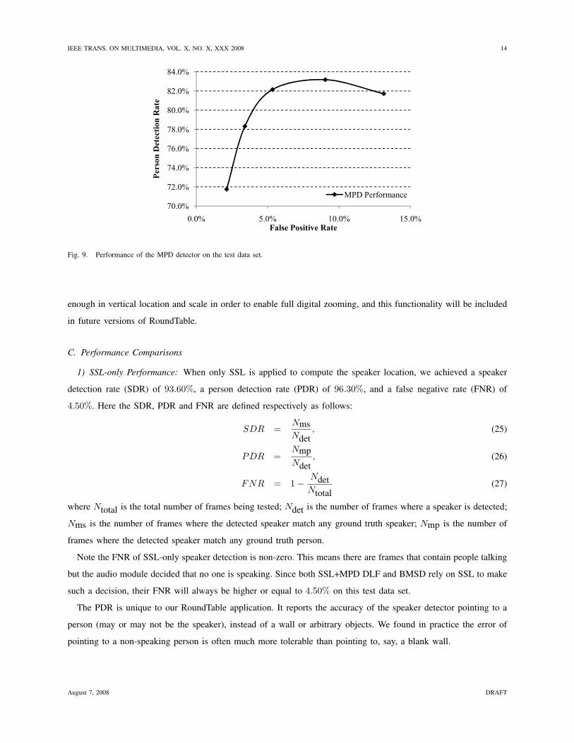
Fig. 9. Performance of the MPD detector on the test data set.

enough in vertical location and scale in order to enable full digital zooming, and this functionality will be included

in future versions of RoundTable.

C. Performance Comparisons

1) SSL-only Performance: When only SSL is applied to compute the speaker location, we achieved a speaker

detection rate (SDR) of 93.60%, a person detection rate (PDR) of 96.30%, and a false negative rate (FNR) of

4.50%. Here the SDR, PDR and FNR are defined respectively as follows:

SDR =NmsNdet

, (25)

PDR =NmpNdet

, (26)

FNR = 1− NdetNtotal

(27)

where Ntotal is the total number of frames being tested; Ndet is the number of frames where a speaker is detected;

Nms is the number of frames where the detected speaker match any ground truth speaker; Nmp is the number of

frames where the detected speaker match any ground truth person.

Note the FNR of SSL-only speaker detection is non-zero. This means there are frames that contain people talking

but the audio module decided that no one is speaking. Since both SSL+MPD DLF and BMSD rely on SSL to make

such a decision, their FNR will always be higher or equal to 4.50% on this test data set.

The PDR is unique to our RoundTable application. It reports the accuracy of the speaker detector pointing to a

person (may or may not be the speaker), instead of a wall or arbitrary objects. We found in practice the error of

pointing to a non-speaking person is often much more tolerable than pointing to, say, a blank wall.

August 7, 2008 DRAFT

IEEE TRANS. ON MULTIMEDIA, VOL. X, NO. X, XXX 2008 15

92.0%

94.0%

96.0%

SDR

86.0%

88.0%

90.0%

4.0% 4.5% 5.0% 5.5% 6.0% 6.5% 7.0%

F�R

SSL only

SSL+MPD, beta = 0.8

SSL+MPD, beta = 0.9

SSL+MPD, beta = 0.95

SSL+MPD, beta = 0.98

Fig. 10. Performance of SSL+MPD decision level fusion on the test data set.

2) SSL+MPD DLF performance: We trained an MPD detector based on the same training data, except that

all the people in the training data set are used as positive examples. Only visual features are selected by the

boosting process. Fig. 9 shows the performance of MPD with 120 visual features (further increasing the number

of features has limited improvements). The horizontal axis is false positive rate, defined as the number of false

positive detections divided by the total number of ground truth person. The vertical axis is person detection rate,

defined as the percentage of people that are accurately detected. Note MPD may output multiple detected person

in each video frame, hence the merging schemes discussed in Section IV-D cannot be applied. We used a scheme

similar to the face detector in [5] for merging the rectangles.

We perform decision level fusion for the SSL and MPD as described in Section IV-E. From Fig. 9, we noted

that the person detection rate of MPD is around 80%, hence we use ε = 0.2 in Eq. (22). By varying the controlling

parameter β and the MPD’s thresholds, we obtained a family of performance curves, as shown in Fig. 10. It can

be seen that the optimal β value for SSL+MPD DLF is around 0.95. The SDR reaches as high as 94.69%, at the

FNR of 5.65%.

The optimal β value is high, which means that more emphasis is given to the SSL instead of the MPD. This

is expected because the MPD’s raw performance is relatively poor. For comparison, we also performed decision

level fusion between SSL and the ground truth labels. Such a fusion is unrealistic, but may provide insights on

what would be the ultimate performance SSL+MPD DLF can achieve (if MPD is perfect). We obtained an SDR

of 95.45% at the FNR of 4.50%.

3) BMSD Performance: The performance of the BMSD detector is summarized in Fig. 11. We used N = 5

for TNM merge. Note the TNM merging algorithm has significantly improved the BMSD’s performance compared

with PAM, in particular when the required FNR is low. This is because when the FNR is low, one must choose to

August 7, 2008 DRAFT

IEEE TRANS. ON MULTIMEDIA, VOL. X, NO. X, XXX 2008 16

90.0%

95.0%

100.0%

SDR

75.0%

80.0%

85.0%

4.00% 5.00% 6.00% 7.00% 8.00% 9.00%

F�R

SSL only

BMSD, PAM merge

BMSD, TNM merge

SSL+MPD, beta=0.95

Fig. 11. Performance of BMSD algorithm on the test data set.

use a very low threshold for the detector. PAM merges all the windows above this threshold, which is error-prone.

In contrast, TNM only picks the top N scored window to merge, which has effectively created an adaptive way to

threshold the scores of the detected windows.

The BMSD outperforms both SSL only and SSL+MPD decision level fusion. At the FNR of 4.50%, BMSD

achieves a SDR value of 95.29%. Compared with the SDR of 93.60% for the SSL only approach, we achieved a

decrease of 24.6% in error. If a higher FNR is acceptable, e.g., at 5.65%, BMSD achieves a SDR value of 95.80%.

Compared with the SDR value of 94.69% for SSL+MPD DLF, the improvement is a decrease of 20.9% in error.

Note the BMSD is also much faster than SSL+MPD, because the BMSD detector uses only 60 features (weak

classifiers), and the MPD uses 120 features.

Fig. 12 shows the person detection rate of the three algorithms on the test data set. As mentioned earlier, the

errors that a speaker detector points to a non-speaking person is much more tolerable than pointing to a blank

wall. It can be seen from Fig. 12 that BMSD outperforms SSL only and SSL+MPD DLF significantly in person

detection rate. Compared with SSL only, at 4.50% FNR, the BMSD’s PDR achieves 98.48% in contrast to 96.30%

for SSL only – a decrease of 58.9% in error. Compared with SSL+MPD DLF, at 5.65% FNR, BMSD has a PDR

value of 98.92% in contrast to 97.77% for SSL+MPD DLF – a decrease of 51.6% in error. For quick reference,

we summarize the performance comparisons between SSL-only, SSL+MPD DLF and BMSD in Fig. 13.

Fig. 14 shows a number of examples of the detection results using BMSD. Fig. 14(a) and (b) are correctly

detected examples, and Fig. 14(c) shows a typical failure example. We notice that most detection failures happen

when the wall reflects the sound waves and causes confusion for the SSL. If there is a person sitting at the same

place where the sound waves are reflected, it is often difficult to find the correct speaker given the low resolution

and frame rate of our visual input. Consequently, slight performance degradation may occur if there are too many

August 7, 2008 DRAFT

IEEE TRANS. ON MULTIMEDIA, VOL. X, NO. X, XXX 2008 17

98.0%

99.0%

100.0%

PDR

95.0%

96.0%

97.0%

4.00% 5.00% 6.00% 7.00% 8.00% 9.00%

F�R

SSL only

BMSD, TNM merge

SSL+MPD, beta=0.95

Fig. 12. Person detection performance of various algorithms on the test data set.

SSL-

only

SSL+MPD

DLFBMSD

Decrease

in error

F�R =

4.50%

SDR 93.60% - 95.29% 24.6%

PDR 96.30% - 98.48% 58.9%

F�R = SDR - 94.69% 95.80% 20.9%F�R =

5.65%

SDR - 94.69% 95.80% 20.9%

PDR - 97.77% 98.92% 51.6%

Fig. 13. Performance comparison table of various algorithms.

people in the room. Fortunately, such a degradation should not cause the algorithm to perform worse than the

SSL-only solution. In Fig. 14(b) BMSD found the correct speaker despite the wrong SSL decision. This is a good

example showing that BMSD is also learning differences between speakers and non-speakers. For instance, the

speakers tend to have more motion than non-speakers.

D. Detection and Speaker Switching Speed

As mentioned in the introduction, the computational complexity is of paramount importance for the design of

the proposed algorithm. Indeed the proposed method is very efficient to compute. On the Taxes Instrument DM642

DSP (600 MHz, 16 bit fixed point), the proposed method with 60 audio/visual features runs comfortably at 3-4 FPS

with a fraction of the computing resource. With a carefully designed cascade pruning method such as that in [36],

our experiments showed that the detector can be tuned to achieve over 15 FPS, which is far beyond our initial goal

of 1 FPS.

August 7, 2008 DRAFT

IEEE TRANS. ON MULTIMEDIA, VOL. X, NO. X, XXX 2008 18

(a)

(b)

(c)

Fig. 14. Examples of the detection results using BMSD. The bars on the top of each image show the strength of SSL likelihood, where the

yellow bar is the peak of the SSL. The dark blue rectangles in the images are the ground truth active speaker, the semi-transparent rectangles

are the raw detection results, and the light green rectangles are the detection results after merging.

It is worth mentioning that an additional layer, namely a virtual director, is needed in order to control the

switching between speakers. While the speaker detector can run up to 15 FPS, research studies have shown that

switching too frequently between shots can be very distracting [2]. In the RoundTable implementation we follow

the simple rule that if the camera has just switched from one speaker to the other, it will stay there for at least 2

seconds before it can switch to another speaker. In addition, a switch is made only if a speaker has been consistently

detected over a period of half a second in order to avoid spontaneous switches due to short comments.

VI. CONCLUSIONS

This paper proposes a boosting-based multimodal speaker detection algorithm that is both accurate and efficient.

We compute audio features from the output of SSL, place them in the same pool as the video features, and let

the logistic AdaBoost algorithm select the best features. To the best of our knowledge, this is the first multimodal

speaker detection algorithm that is deployed in commercial products.

The current RoundTable system can only detect a single speaker at any time due to the top N merge algorithm

presented in Section IV-D. In principle, multiple speakers can be detected with the same approach using a more

traditional merge method (such as the one in [5]). In practice, however, there are a few challenges. For instance, the

labeling process can be very error-prone if all speakers speaking simultaneously are to be labeled – multi-speaker

detection could be a challenging task for humans too, in particular when the video resolution is very low. The SSL

algorithm described in Section III is designed for single sound source only. New efficient algorithms need to be

designed to locate multiple sources, which is still a research topic. Finally, detecting multiple speakers in the same

video frame shall require a much higher accuracy in the raw detector’s performance. Additional, more complex

August 7, 2008 DRAFT

IEEE TRANS. ON MULTIMEDIA, VOL. X, NO. X, XXX 2008 19

features such as histogram of oriented gradients [37] may be explored. We will study these challenges in our future

work.

REFERENCES

[1] C. Busso, S. Hernanz, C. Chu, S. Kwon, S. Lee, P. Georgiou, I. Cohen, and S. Narayanan, “Smart room: participant and speaker localization

and identification,” in Proc. of IEEE ICASSP, 2005.

[2] R. Cutler, Y. Rui, A. Gupta, J. Cadiz, I. Tashev, L. He, A. Colburn, Z. Zhang, Z. Liu, and S. Silverbert, “Distributed meetings: a meeting

capture and broadcasting system,” in Proc. ACM Conf. on Multimedia, 2002.

[3] B. Kapralos, M. Jenkin, and E. Milios, “Audio-visual localization of multiple speakers in a video teleconferencing setting,” York University,

Canada, Tech. Rep., 2002.

[4] B. Yoshimi and G. Pingali, “A multimodal speaker detection and tracking system for teleconferencing,” in Proc. ACM Conf. on Multimedia,

2002.

[5] P. Viola and M. Jones, “Robust real-time face detection,” Int. Journal of Computer Vision, vol. 57, no. 2, pp. 137–154, 2004.

[6] H. Wang and P. Chu, “Voice source localization for automatic camera pointing system in videoconferencing,” in Proc. of IEEE ICASSP,

1997.

[7] Y. Rui, D. Florencio, W. Lam, and J. Su, “Sound source localization for circular arrays of directional microphones,” in Proc. of IEEE

ICASSP, 2005.

[8] A. Adjoudani and C. Benoıt, “On the integration of auditory and visual parameters in an HMM-based ASR,” in Speechreading by Humans

and Machines. Springer, Berlin, 1996, pp. 461–471.

[9] S. Dupont and J. Luettin, “Audio-visual speech modeling for continuous speech recognition,” IEEE Trans. on Multimedia, vol. 2, no. 3,

pp. 141–151, 2000.

[10] W. Hsu, S.-F. Chang, C.-W. Huang, L. Kennedy, C.-Y. Lin, and G. Iyengar, “Discovery and fusion of salient multi-modal features towards

news story segmentation,” in SPIE Electronic Imaging, 2004.

[11] M. Brand, N. Oliver, and A. Pentland, “Coupled hidden Markov models for complex action recognition,” in Proc. of IEEE CVPR, 1997.

[12] M. Naphade, A. Garg, and T. Huang, “Duration dependent input output Markov models for audio-visual event detection,” in Proc. of IEEE

ICME, 2001.

[13] G.Iyengar and C.Neti, “Speaker change detection using joint audio-visual statistics,” in The Int. RIAO Conference, 2000.

[14] P. Besson and M. Kunt, “Information theoretic optimization of audio features for multimodal speaker detection,” Signal Processing Institute,

EPFL, Tech. Rep., 2005.

[15] J. Fisher III, T. Darrell, W. Freeman, and P. Viola, “Learning joint statistical models for audio-visual fusion and segregation,” in NIPS,

2000, pp. 772–778.

[16] J. Hershey and J. Movellan, “Audio vision: using audio-visual synchrony to locate sounds,” in Advances in Neural Information Processing

Systems, 2000.

[17] V. Pavlovic, A. Garg, J. Rehg, and T. Huang, “Multimodal speaker detection using error feedback dynamic Bayesian networks,” in Proc.

of IEEE CVPR, 2001.

[18] D. N. Zotkin, R. Duraiswami, and L. S. Davis, “Logistic regression, adaboost and bregman distances,” EURASIP Journal on Applied

Signal Processing, vol. 2002, no. 11, pp. 1154–1164, 2002.

[19] J. Vermaak, M. Gangnet, A. Black, and P. Perez, “Sequential Monte Carlo fusion of sound and vision for speaker tracking,” in Proc. of

IEEE ICCV, 2001.

[20] H. Nock, G. Iyengar, and C. Neti, “Speaker localisation using audio-visual synchrony: an empirical study,” in Proc. of CIVR, 2003.

[21] R. Cutler and L. Davis, “Look who’s talking: speaker detection using video and audio correlation,” in Proc. of IEEE ICME, 2000.

[22] M. Beal, H. Attias, and N. Jojic, “Audio-video sensor fusion with probabilistic graphical models,” in Proc. of ECCV, 2002.

[23] Y. Chen and Y. Rui, “Real-time speaker tracking using particle filter sensor fusion,” Proceedings of the IEEE, vol. 92, no. 3, pp. 485–494,

2004.

[24] K. Nickel, T. Gehrig, R. Stiefelhagen, and J. McDonough, “A joint particle filter for audio-visual speaker tracking,” in ICMI, 2005.

[25] C. Zhang, Z. Zhang, and D. Florencio, “Maximum likelihood sound source localization for multiple directional microphones,” in ICASSP,

2007.

August 7, 2008 DRAFT

IEEE TRANS. ON MULTIMEDIA, VOL. X, NO. X, XXX 2008 20

[26] T. Gustafsson, B. Rao, and M. Trivedi, “Source localization in reverberant environments: performance bounds and ml estimation,” in Proc.

of ICASSP, 2001.

[27] M. Brandstein and H. Silverman, “A robust method for speech signal time-delay estimation in reverberant rooms,” in Proc. of ICASSP,

1997.

[28] J. Friedman, T. Hastie, and R. Tibshirani, “Additive logistic regression: a statistical view of boosting,” Dept. of Statistics, Stanford University,

Tech. Rep., 1998.

[29] R. Schapire and Y. Singer, “Improved boosting algorithms using confidence-rated predictions,” Machine Learning, vol. 37, no. 3, pp.

297–336, 1999.

[30] P. Viola, M. Jones, and D. Snow, “Detecting pedestrians using patterns of motion and appearance,” in Proc. of IEEE ICCV, 2003.

[31] R. Collins, A. Lipton, T. Kanade, H. Fujiyoshi, D. Duggins, Y. Tsin, D. Tolliver, N. Enomoto, and O. Hasegawa, “A system for video

surveillance and monitoring,” Robotics Institute, Carnegie Mellon University, Tech. Rep., 2000.

[32] C. Wren, A. Azarbayejani, T. Darrell, and A. Pentland, “Pfinder: real-time tracking of the human body,” IEEE Trans. on PAMI, vol. 19,

no. 7, pp. 780–785, 1997.

[33] S. Goodridge, “Multimedia sensor fusion for intelligent camera control and human computer interaction,” Ph.D. dissertation, Department

of Electrical Engineering, North Carolina Start University, 1997.

[34] M. Collins, R. Schapire, and Y. Singer, “Logistic regression, adaboost and bregman distances,” Machine Learning, vol. 48, no. 1-3, pp.

253–285, 2002.

[35] L. Mason, J. Baxter, P. Bartlett, and M. Frean, “Boosting algorithms as gradient decent,” in NIPS, 2000.

[36] C. Zhang and P. Viola, “Multiple-instance pruning for learning efficient cascade detectors,” in NIPS, 2007.

[37] N. Dalal and B. Triggs, “Histograms of oriented gradients for human detection,” in Proc. of CVPR, 2005.

August 7, 2008 DRAFT