boosting decision stumps for dynamic feature selection on

Boosting Decision Stumps for Dynamic Feature

Selection on Data Streams

Jean Paul Barddal, Fabrıcio Enembreck

Graduate Program in Informatics (PPGIa) – Pontifıcia Universidade Catolica do Parana

Heitor Murilo Gomes, Albert Bifet

INFRES, Institut Mines-Telecom, Telecom ParisTech, Universite Paris-Saclay, Paris,

France

Bernhard Pfahringer

Department of Computer Science – University of Waikato

Abstract

Feature selection targets the identification of which features of a dataset arerelevant to the learning task. It is also widely known and used to improvecomputation times, reduce computation requirements, and to decrease theimpact of the curse of dimensionality and enhancing the generalization ratesof classifiers. In data streams, classifiers shall benefit from all the itemsabove, but more importantly, from the fact that the relevant subset of fea-tures may drift over time. In this paper, we propose a novel dynamic featureselection method for data streams called Adaptive Boosting for Feature Se-lection (ABFS). ABFS chains decision stumps and drift detectors, and as aresult, identifies which features are relevant to the learning task as the streamprogresses with reasonable success. In addition to our proposed algorithm,we bring feature selection-specific metrics from batch learning to streamingscenarios. Next, we evaluate ABFS according to these metrics in both syn-thetic and real-world scenarios. As a result, ABFS improves the classificationrates of different types of learners and eventually enhances computational re-

Email addresses: jean.barddal, [email protected] (Jean PaulBarddal, Fabrıcio Enembreck), heitor.gomes, [email protected]

(Heitor Murilo Gomes, Albert Bifet), [email protected] (BernhardPfahringer)

Preprint submitted to Information Systems January 7, 2019

sources usage.

Keywords: Data Stream Mining, Feature Selection, Concept Drift, FeatureDrift

1. Introduction

Feature selection is an essential part of a machine learning pipeline. Thecentral goal of this task is to identify and retain the subset of features of adataset that is relevant to the learning task. Despite its benefits to reducecomputation time by focusing the model training only on a subset of features,feature selection can have an even bigger impact in diminishing the curse ofdimensionality. This characteristic can enhance the performance of predictivemodels. Comparing the feature selection studies from the last 20 years, thenumber of dimensions (features) has rapidly grown. For instance, the studiesof [1, 2] tackled datasets described with an average of 40 features. In the ageof Big Data, the number of features has grown tremendously, where hundreds,thousands [3] or even millions of them are observed in specific domains [4],and these are called high-dimensional scenarios.

Traditional feature selection techniques are tailored to be part of the pre-processing step of the batch knowledge discovery process. Nevertheless, avariety of data mining applications are not static, as data often arrive inthe form of potentially infinite sequences of data, the so-called data streams.Learning from data streams exhibits not only the challenges from traditionallearning schemes, e.g., missing values and class imbalance; but also conceptdrifts. A concept drift occurs when the data distribution changes, possiblyimpacting the relationship of features, their values, and the target variable[5].

Recently, studies on data stream mining shed light on the fact that certaintypes of drift affect the importance of features over time. Scenarios wherefeatures become, or cease to be, relevant to the learning task are called featuredrifting data streams, and these are the target of this paper.

In this paper, we propose a novel dynamic feature selection method fordata streams called Adaptive Boosting for Streaming Feature Selection. Ourproposal is tailored to tackle feature drifting high-dimensionality scenarios,thus allowing classifiers to learn from a reduced number of features. Thismethod adopts a boosting scheme inspired by the work of [6] with decisionstumps to dynamically identify which features are relevant to the current

2

concept of a data stream. Drift detectors are used to flag drifts and enablequick response to changes in the importance of features. We evaluate ourproposal in a variety of streaming scenarios, and also with different typesof learners. Additionally, we show how metrics from batch feature selectioncan be ported to streaming scenarios. These metrics, along with the code forour proposed method, are made available for the community1 as part of theMassive Online Analysis (MOA) software [7].

This paper is divided as follows. Section 2 introduces the data streamclassification and feature drifts. Section 3 reviews related work on featureanalysis in data streams. Section 4 introduces our proposal, namely AdaptiveBoosting for Feature Selection (ABFS), while Section 5 conducts an analysison how feature selection-specific evaluation metrics can be used in streamingscenarios. Next, in Section 6, the proposed method is evaluated againstdifferent base learners, showing its efficacy and efficiency in a variety of datastreams and dimensions. Finally, Section 7 concludes this paper.

2. Problem Statement

In this paper, we target the classification task for inductive learning fromdata streams. More formally, let S to be a data stream providing instances(~x1, y1), . . ., (~xt, yt) as t → ∞. We also denote ~xt to be a d-dimensionalfeature vector belonging to a feature set F =

⋃di=1 fi, and Y =

⋃ci=1 yi

to be the set of c possible class labels. In data stream classification, our goalis to continuously learn and update a model h : ~x → y that maps featuresand their values to class labels as new data becomes available.

One of the most important traits of data streams is that their underlyingdistribution may change over time. As a result, these changes affect theconcept to be learned; a phenomenon referred to as concept drift. In thispaper, we target a specific type of concept drift that occurs when featuresbecome, or cease to be, relevant to the learning task. In the seminal work of[5], this type of drift was referred to as contextual concept drift, while morerecent works [8, 9] call it feature drift. In contrast to conventional conceptdrifts, where changes occur in the relationship between values or ranges of

1The code for our implementation of ABFS, data generators, evaluation metrics, andscripts to reproduce the experiments shown in this paper are available at https://github.com/jpbarddal/moa-abfs.

3

variables and the class, feature drifts occur whenever a subset of featuresbecomes or ceases to be relevant for the current concept to be learned.

Formally, we divide features in two types: relevant and irrelevant accord-ing to the work of [8]. Assuming Si = F \ fi, a feature fi is deemedrelevant iff Equation 1 holds.

∃S ′i ⊂ Si, such that P [Y |fi, S ′i] 6= P [Y |S ′i] (1)

Otherwise, the feature fi is said irrelevant. In practice, if a feature thatis statistically relevant is removed from a feature set, it will reduce overallprediction power since (i) it is strongly correlated with the class; or (ii) itbelongs to a subset of features that is strongly correlated with the class [10].

According to the previous definitions, if a feature that is statisticallyrelevant is removed from a feature set, it will reduce overall prediction power.This definition encompasses two possibilities for a feature to be statisticallysignificant: (i) it alone is strongly correlated with the class; or (ii) it forms afeature subset with other features and this subset is strongly correlated withthe class [11, 10].

In streaming scenarios, changes in the relevant subset of features force thelearning process to adapt its model accordingly [12]. Given a feature spaceF at a timestamp tj, we denote F∗tj as its ground-truth relevant subset offeatures such that ∀fi ∈ F∗tj the aforementioned definition of relevance holds.Therefore, a feature drift occurs if between two timestamps tj and tk we findthat F∗tj 6= F

∗tk

.To overcome this type of drift, a classifier must identify these relevance

changes, and either (i) discard and learn a new model with the newly relevantfeatures, or (ii) adapt its current model to relevance drifts [12].

3. Related Work

Finding a compact subset of relevant features is a widely tackled problemof batch learning, yet, the same does not hold for streaming scenarios. Atthis point, it is relevant to disclaim that this is different from online featureselection, which is the task that targets the identification of the best subset offeatures in a very high-dimensional space (hundreds of thousands or millionsof dimensions), which is a typical problem of big data [13, 14]. Although bothtasks’ objectives overlap in the sense that both tackle the issue of featureselection, streaming feature selection receives as input a stream of features

4

(not instances), and their inclusion in the model is performed sequentially,without observing future features [15]. In contrast, our goal in this paperis to dynamically select features in streaming scenarios where new instancesbecome available over time and the original feature set is static.

Recently, the works of [16] and [17] surveyed and evaluated different ap-proaches to tackle this problem. According to these studies, incremental de-cision trees [18] and its variants [19] are the best performing approaches. De-cision trees can be regarded as feature selection processes since they continu-ously select the feature that maximizes a quality metric during the branchingstep. For instance, the Hoeffding Tree [18] collects statistics about incom-ing data, and periodically, according to a grace period parameter, determinewhich feature should be used to split the tree and create even more specificleaf nodes. One of the significant drawbacks of the conventional HoeffdingTree learner is that it is purely incremental as it does not check if any of theprevious splits are still accurate. To overcome this issue, the Hoeffding Adap-tive Tree [19] uses the ADWIN drift detector [20] inside decision nodes tomonitor the internal error rates of the tree, and re-learn branches if needed.

Another recent work that focused on performing feature selection is theHeterogeneous Ensemble with Feature Drift for Data Streams (HEFT-Stream)[12]. HEFT-Stream incorporates traditional feature selection into a hetero-geneous ensemble to adapt to different types of concept and feature drifts.HEFT-Stream adopts a modification of the Fast Correlation-Based Filter(FCBF) algorithm so it dynamically updates the selected relevant featuresubset of a data stream. The main shortcoming of HEFT-Stream is that isprocesses the data stream using mini-batches, and the determination of thesize of such batches is left to the user. To perform the scoring of featuresover sliding windows, the work of [8] proposes a dynamic feature weightingscheme for the streaming versions of Naive Bayes and k-Nearest Neighbors.Weights are computed with sliding window formulas for the SymmetricalUncertainty scoring operator [21] and are used in the prediction step of thelearners mentioned above. The accuracy gains are noticeable despite theexpense of reasonable processing time and memory usage. Finally, the pro-posed weighting scheme was used at the leaves of the Hoeffding AdaptiveTree to improve its prediction rates, again with a computational overhead.

Another relevant approach is given in the work of [22], where authorsproposed an unsupervised approach for feature ranking, and posterior selec-tion, based on Frequent Directions. In practice, their proposal operates ina streaming by constructing and maintaining a sketch matrix that shrinks

5

the original data in orthogonal vectors. Even though the results obtained interms of feature selection are interesting, authors work under the assumptionthat the number of features to be selected is known a priori and that theuser is able to provide this number correctly.

At this point, it is worthy to notice that measuring the importance offeatures on streaming regression scenarios has also gained traction in thework of [23], yet, no feature selection proposals are provided. And finally, itis also relevant to mention that our main goal in this paper is to introducea feature selection method for data streams that is not highly dependent ofa user-given window size. This is relevant since, in practice, any traditionalfeature selection method can be applied to data streams by partitioning thearriving data in chunks of size n. At the end of each chunk, traditionalfeature selection methods could then be applied to the n previously instancesgathered, thus resulting in a feature set that would be used to build a classifierto predict the upcoming n instances. Naturally, the biggest issue here is howto determine an appropriate value for n, and this problem is referred to as theplasticity-stability dilemma. While short windows reflect the current datadistribution and ensure fast adaptation to drifts (plasticity), they usuallyworsen the performance of the system in stable areas. Conversely, largerwindows give better performance in stable periods (stability), however, theseimply in slower reaction to drifts [24].

4. Proposed Method

In this section, we propose a novel method based on Online Boosting [6]and drift detectors to identify which features are relevant for the classificationtask on data streams. We start this section with an introduction to Boostingmethods for both batch and stream learning settings. These methods are atthe core of the proposed method as Boosting allows feature interactions tobe swiftly identified in data streams. The next part describes the proposedmethod and discusses its functioning. At this point, it is important to high-light that even though the proposed method has its foundations borrowedfrom [6], it is not tailored for classification as its inner weak learners are notused during predictions; and no convergence with batch learning is reportedfor the same reason.

6

4.1. Preliminaries on boosting

In machine learning, Boosting is a family of meta-learning methods thattarget the construction of a strong learner by combining multiple weak learn-ers that, by definition, are slightly better than random guessing.

The most widely used and known implementation of Boosting is Ad-aBoost [25], and multiple variants of it were proposed throughout the years[26, 27]. In AdaBoost, a set of weak learners H is trained over a series ofrounds t = 1, . . . , T . During each iteration, a new weak learner ht : ~x → yis trained over the dataset (~x1, y1), . . . , (~xn, yn) taking into account a distri-bution of weights Dt for these instances. In the first round, it is assumedthat all instances have the same weight, i.e. D1(i) = 1

n. The error of a weak

learner in the t-th round is the sum of the weights of misclassified instances,as shown in Equation 2.

εt = Pri∼Dt

[ht(~x

i) 6= yi]

=∑

∀i,ht(~xi)6=yiDt(i) (2)

In each of the following rounds, the weights Dt(i) are updated accordingto a parameter αt, which is calculated according to Equation 3.

αt =1

2ln

(1− εtεt

)(3)

In practice, αt quantifies how “important” ht is, as αt ≥ 0 if εt ≤ 1/2and that αt increases with the decrease of εt. According to αt, the weightdistribution can be updated following Equation 4, where Zt =

∑ni Dt(i) is a

normalization factor to guarantee that Dt is a distribution.

Dt+1(i) =Dt(i)

Zt×

e−αt if ht(~x

i) = yi

eαt if ht(~xi) 6= yi

(4)

With this update, the weights of correctly classified instances will de-crease, while misclassified instances will increase. As a result, this processhighlights hard-to-classify instances for future rounds.

Finally, predictions can be extracted from the final “strong” learner asdepicted in Equation 52.

2The original prediction scheme presented in [28] focuses only on binary classificationtasks and has been extended here to account for multi-class problems. Details about the

7

H(~x) = arg maxyi∈Y

(T∑t=1

αtht(~x) if ht(~x) = yi

0 if ht(~x) 6= yi

)(5)

Even though AdaBoost is iterative, it works under the assumption thatall instances of the dataset are available at all times so that re-weightingoccurs. Naturally, this is an assumption that does not hold in streamingscenarios, as each instance should be processed and discarded right after.Targeting the development of boosting techniques for data streams, differentapproaches for classification [6, 29, 30] and regression [31] tasks have beendeveloped over the years.

In this work, we follow a similar framework proposed in [6], called Oza-Boost. OzaBoost was tailored to be an approximation of AdaBoost for datastreams. Contrary to AdaBoost, where the number of rounds T determinesthe ensemble size, OzaBoost has a predefined number of weak learners Mand counters for correctly (λci , 1 < i < M) and incorrectly (λei , 1 < i < M)classified instances which are updated as new instances are processed. Foreach instance (~xt, yt) drawn from the data stream S, a weight λ = 1 is set.The instance is then traversed along the weak learners h1, . . . , hM sequen-tially. For each hi, the instance is tested to check whether if it is correctlyclassified or not, i.e. hi(~x

t) = yt or not; and as a result, the counters λci andλei are incremented with λ (Equations 6 and 7, respectively). Next, the valueof λ is incremented or decremented following Equation 8. This is the sameprocedure adopted by AdaBoost in Equations 4 and 5, except the normaliza-tion factor Zt, which cannot be used in data streams as past instances havebeen discarded.

λci ← λci + λ; (6)

λei ← λei + λ; (7)

λ← λ×

λci+λ

ei

2λciif hi(~x) = yt

λci+λei

2λeiif hi(~x) 6= yt

(8)

usage of AdaBoost in binary classification tasks and proofs on its error bounds can alsobe found in the same paper.

8

4.2. Adaptive Boosting for Feature Selection

The properties of boosting have been investigated to improve classifica-tion rates, but also as a proxy for feature selection in batch scenarios. Forinstance, the work of [32] uses gradient boosted regression trees to select fea-tures. Also, related to our approach, authors in both [33] and [34] proposeddifferent boosting techniques that use decision stumps to select features inbatch scenarios.

We now propose a novel method based on Boosting to dynamically selectfeatures in streaming scenarios hereafter referred to as Adaptive Boosting forFeature Selection (ABFS). At this point, it is important to disclaim thatthe term Adaptive used here stands for the fact that the proposed methodincrementally selects features as the stream is processed, but it is also ableto detect feature drifts and adapt to them on the fly.

ABFS combines decision stumps and drift detectors to perform dynamicfeature selection. Decision stumps are light-weighted, incremental, easy toimplement and understand, but more importantly, an elegant approach toidentify which feature maximizes a purity criterion and selects a feature ac-cordingly. Below, we describe each of these components individually andlater how they are chained together to allow dynamic feature selection indata streams.

4.2.1. Decision stumps

The decision stump implementation used here is the core unit of incre-mental decision trees, e.g., Hoeffding Trees [18], and receive as input threeparameters: a selection threshold θ, a grace period gp and a purity metricΩ(·) that we wish to maximize, e.g. Information Gain and Gini Index. Bydefinition, a decision stump ds gathers statistics on the arriving data untilthe grace period gp is reached. After that, all features fi ∈ F are evaluatedaccording to a criterion Ω(·). Let fα and fβ be the two best-ranked featuresaccording to Ω. As proposed in [18], a decision stump will split on fα ifΩ(fα) − Ω(fβ) > ε, where ε is the Hoeffding bound [35], given by Equation9, and R is the range of Ω.

ε =

√R2 ln

(1δ

)2× gp

(9)

As in [18], the Hoeffding bound is used to approximate how many samplesare required to achieve the optimal selection of a feature that would occur if

9

the entire data stream was observed. As a result, with probability (1 − δ),it is statistically valid that fα is the best feature to be selected [18]. It isalso possible that during this evaluation, two or more features show similarΩ values, and thus, the number of examples required to decide between themwith high confidence may grow indefinitely. Naturally, this is unwanted, asthe gain obtained by either makes little difference, i.e., such features arelikely to be redundant; and thus, the proposed implementation for decisionstumps follows the Hoeffding Tree protocol where a parameter τ is used fortie-breaking [18]. Following the definition of [18] and [7], the tie-breakingparameter was set as τ = 0.05 for all of the experiments conducted in thispaper. In practice, the decision stump will select the best-ranked feature fαif τ > Ω(fα)− Ω(fβ) > ε.

In the proposed method, the decision stump is extended in two aspects.First, a decision stump will select the most appropriate feature fα from asubset of features that have not been previously selected by other decisionstumps. The idea on using boosting with decision stumps is that by travers-ing each instance across all the boosting units, instances that are hard toclassify will be highlighted and will force the decision stump that is aboutto split to select a feature that better separates such samples. And second,the best-ranked feature fα will only be selected if Ω(fα) > θ, which is a user-given threshold. Naturally, the definition of a selection threshold θ dependson the data domain being worked on, and different values are evaluated inSection 6.

4.2.2. Drift detectors

A drift detector is a statistical method that observes a data sequence andupon on its distribution, flags the occurrence of significant changes. In datastreams, most of the drift detectors are used to monitor the error rates ofa classifier. In this work, we denote ψ to be a drift detector that receivesas input a value of 1 if h(~xt) 6= yt, or 0 otherwise. Evidently, differentrealizations of ψ exist, e.g. ADWIN [19], HDDM-A and HDDM-W [36]; andthe impact of different techniques are also assessed in Section 6.

ADWIN is, by far, the most popular choice for drift detection. It keepsa variable-length window of recently seen items, with the property that thewindow has the maximal length statistically consistent with the hypothesis“there has been no change in the average value inside the window”. TheADWIN change detector is parameter- and assumption-free in sense that itautomatically detects and adapts to the current rate of change. In the average

10

case, the cost of processing each instance by ADWIN is instantaneous, whilein the worst case it can be of O(logW ), where W is the size of the slidingwindow maintained in memory.

More recently, the authors in [36] proposed two variants of the HoeffdingDrift Detection Method (HDDM) detector: HDDM-A and HDDM-W. Boththe former and the latter are similar to ECDD in the sense that they usemoving averages to detect drifts, yet, only the latter uses an exponentiallyweighted procedure to provide higher importance to most recent data. Inboth cases, the moving averages are compared to flag concept drifts basedon the misclassification rates of a classifier, where the Hoeffding Bound (seeEquation 9) is used to set an upper bound to the accepted level of differencebetween them. In contrast to ADWIN, the complexity for both HDDM-Aand HDDM-W is of O(1) in the worst case.

4.2.3. Chaining decision stumps and drift detectors in a boosting scheme

The rationale behind ABFS is that boosting gives more weight to in-stances that are hard to classify. By intuition, these instances are either (i)located at the decision boundaries of classes, or (ii) are noise. If we workunder the assumption that the labels of incoming instances are trustworthy(not noisy), decision stumps will be able to select the most important fea-tures according to these hard-to-classify instances as they naturally accountfor these weights during the feature selection process. In ABFS, each decisionstump will be responsible for finding the feature that maximizes the meritfunction Ω without observing features that have been selected previously.

Since ABFS was tailored for feature selection in classification scenariosand not for actually training classifiers, we will adopt a slightly differentnotation from the boosting schemes presented earlier. ABFS is composed ofa dynamic set of boosting units U such that each unit ui ∈ U is a 4-tuplein the (dsi, λ

ci , λ

ei , ψi) form, where dsi is a decision stump, λci and λei are

counters for correctly and incorrectly classified instances by dsi and ψi is adrift detector. The functioning of ABFS is detailed in Algorithm 1 and isdivided into 3 steps: initialization, training, and selection.

In the initialization step (lines 1-4 of Algorithm 1), ABFS instantiatesboth the set of boosting units U and the subset of selected features F ′ asempty lists, a candidate decision stump dscandidate that will gather statisticsabout incoming data to determine which feature to split on and select.

During the training step (lines 5-31 of Algorithm 1), ABFS updates itsinternal structures according to the arrival of an instance (~xt, yt). First, the

11

instance weight λ and an index to store the first layer that detects a drift idriftare initialized. Next, the arriving instance is sequentially traversed along allof the boosting units in U . In each boosting unit ui = (dsi, λ

ci , λ

ei , ψi), it

is verified if the decision stump is able to correctly predict the class label(dsi(~x

t) = yt), or not (dsi(~x) 6= yt). Here, AdaBoost’s weighting strategy isfollowed (Equations 6, 7 and 8), where higher values of λ will be associatedwith instances that are hard to classify. It is also important to highlight thatafter the classification of the instance in a unit ui, the selected feature usedin its decision stump dsi is removed from ~x (line 20) so that the candidatedecision stump dscandidate is enforced to select a feature that has not beenselected already by the decision stumps in U .

In addition to the definition of λ, the drift detector is fed with the classifi-cation result (1 represents an error, while 0 represents a correct classification).Therefore, each drift detector is used to keep track of the error distribution ofeach decision stump. The rationale here is that changes in these distributionswork as a proxy to identify when the importance of a feature changes, andthus, upon the flagging of a drift, it becomes necessary to re-start the featureselection process. In practice, if a drift is flagged by ψi, its index i will bestored in idrift so that this and the following units are removed, and thatthe feature selection process can self-adjust upon the new data distribution.Naturally, depending on the drift, it would be possible that multiple unitsflag drifts, and thus, only the first layer that detects such changes is stored.

If no changes are detected (lines 21 to 26), the candidate decision stumpdscandidate is trained3 with (~xt, yt) assuming a weight λ. With the arrival ofmultiple instances, the candidate decision stump will reach the grace periodgp, and as a result, it will eventually select a new feature fα according tothe process described earlier. When this condition holds, a new boostingunit is instantiated with this decision stump, and it is added to U . A newcandidate decision stump is then created to select the next best feature, andthe selected subset of features is incremented with fα.

On the other hand, it is, a feature drift is detected, all boosting unitsfrom the index that detected the change until the end of the list are removed(loop described by lines 28 and 29), as a boosting unit ui affected the creationof its following units ∀uj, j ≥ i. Next, and the classifier h is reset to allow

3In decision stumps, whenever an instance (~xt, yt) is used for training with a weight λ,it means that the same instance has been observed λ times

12

Algorithm 1 ABFS pseudocode. We denote h to be a pointer to the classi-fier, dscandidate a candidate decision stump, F ′ the currently selected subsetof features, θ a selection threshold used in decision stumps, and U the setof boosting units such that the ui is the i-th unit and it is composed of adecision stump dsi, a set of counters for correctly (λci) and misclassified (λei )instances, and a drift detector ψi.

1: procedure INITIALIZE(h, F , θ)2: U ← ∅;3: dscandidate ← new DecisionStump(θ);4: F ′ ← ∅;5: procedure TRAIN(~xt, yt)6: λ← 1;7: idrift ← −1;8: for i← 1 to |U | do9: if dsi(~x

t) = yt then10: λci ← λci + λ;

11: λ← λ× λci+λei

2λci;

12: Update ψi with 0;13: else14: λei ← λei + λ;

15: λ← λ× λci+λei

2λei;

16: Update ψi with 1;

17: if ψi flagged a drift and idrift = −1 then18: idrift ← i;19: break;

20: Remove from ~x the feature selected at dsi;

21: if idrift = −1 then22: Train dscandidate with (~xt, yt) assuming a weight λ;23: if dscandidate has selected a feature fα ∈ F then24: U ← U ∪ new BoostingUnit(dscandidate);25: dscandidate ← new DecisionStump(θ);26: F ′ ← F ′ ∪ fα;27: else28: while |U | > idrift do29: Remove from F ′ the feature selected in U.last();30: U ← U \ U.last();31: Reset the learner h;

32: procedure SELECT(~x)33: return ~x after selecting the features selected in F ′ and dropping the

remainder of the features;

13

faster adaptation to the new concept. In practice, the reset of a classifierstands for the process in which its model is discarded and the learners startsto learn from scratch.

Finally, the last part is the testing step (lines 32 and 33 of Algorithm1), ABFS filters the arriving instance ~x so that only the features in F ′ areselected. This instance can then be passed to the classifier with a reduceddimensionality equals to |F ′|.

4.2.4. A note on complexity analysis

The initialization step of ABFS is trivial, as it simply instantiates therequired structures, which results in O(1). Naturally, the most computation-ally intensive part of ABFS is training step. In practice, the upper boundcost of ABFS is given by the loop described by lines 8 to 20 of Algorithm 1,which basically loops over all the boosting units in U , which has the samecardinality as the subset of selected features F ′. Inside this loop, the con-ditions described by lines 9-12 and 13-16 are mutually exclusive and havethe same cost, which is basically described by the cost of the drift detectorupdate, which is O(logW ) for ADWIN and O(1) for HDDM-A and HDDM-W. Next, another important aspect of ABFS occurs in line 22, where theupdate of a decision stump has a cost of O(d−U), as it needs to loop over allthe unselected features. Similarly, the condition described in line 23, wherea feature is selected requires (d − U) computations of Information Gain,but these are precomputed as statistics are incrementally updated, but also(d− U) log2(d− U) computations so that the features are sorted. Yet, suchcomputation only occurs every gp instances, and thus, the computationalcost becomes O( (d−U) log2(d−U)

gp). On the other hand, if a drift is flagged in

line 27, the cost in the worst case occurs with the removal of all features thathave been selected, and thus, the cost is of O(U). Given that, the overall

cost for ABFS is of O(U logW +(d−U)+ (d−U) log2(d−U)gp

), which after simpli-

fication becomes O(U logW + (d−U) log2(d−U)gp

). Also, since the average cost of

ADWIN is pessimistic, one could also assume O(U +(d−U)+ (d−U) log2(d−U)gp

)instead. Finally, the selection step is also simple, as it builds a new instanceby iterating over the selected subset of features F ′, and thus, with a cost ofO(U).

14

5. Evaluating Feature Selection on Data Streams

There are different factors to account for when evaluating feature selectionproposals. Throughout the years, different quantitative measures, such asaccuracy and scalability, and subjective ones, such as ‘ease of use’, have beenused to highlight the efficiency of feature selectors [37]. In this paper, wedefine a quantitative framework to evaluate our proposal and future workson feature selection for data streams. This framework includes (i) accuracy,(ii) processing time, (iii) memory usage, (iv) selection accuracy; and (v)stability metrics. Metrics (i) through (iii) are widely used in the area as theyfollow traditional data stream evaluation frameworks [38] for the assessmentof classifiers. Metrics (iv) and (v) are absent in streaming scenarios as bothSelection Accuracy and Stability metrics were developed for batch scenarios.The following sections present these metrics and discuss their computationon data streams. Along the proposed method, the implementation of thesemetrics is also provided to the data stream mining community as part of theMassive Online Analysis (MOA) software [7].

5.1. Selection Accuracy

Selection Accuracy (SA) is a classifier-independent score that quantifiesto what extent a selected subset of features matches the ground-truth relevantones [39]. Given a feature set F , its relevant subset of features F∗ and theselected set F ′ ⊆ F , SA is given by Equation 10, where γ ∈ [0; 1] is aweighting factor and its output is also bounded in [0; 1].

SA(F ,F∗,F ′) = γ

RRF︷︸︸︷(|F∗ ∩ F ′||F∗|

)+(1− γ)

(1− |(F \ F

∗) ∩ F ′||F| − |F∗|

)︸︷︷︸

CCP

(10)

A score of SA = 1 corresponds to a perfect selection, where all the relevantset of features is selected, and no extraneous features are retained; whereasSA = 0 represents the opposite, i.e., a selection with no relevant features andall extraneous ones selected. One of the main advantages of SA is that theinformation on the degree to which a model has been correctly or incorrectlyspecified is combined into a single value, thus making the comparison betweenseveral feature selection proposals clear and classifier-independent.

15

The computation of SA also requires an appropriate γ. This choice issubjective and depends on how much one wants to favor accuracy over par-simony or vice-versa. Hereafter, the two components that compose the SAformula are referred as Recall of Relevant Features (RRF ) and Complementof Complexity Penalty (CCP ). A suitable value for γ should reflect the factthat choosing an extraneous feature is usually better than missing a relevantone, something that can be achieved by selecting γ, such that γ

|X∗| >1−γ

|X|−|X∗|[39]. On the other hand, γ should not be too large, as that would resultin insignificant penalties for unnecessarily complex models. Authors in [37]provided an empirical evaluation of different values of γ and claimed that 0.7is an appropriate value since it satisfies the condition mentioned above whilebeing sufficiently less than 1 to appropriately penalize unnecessary complex-ity.

The advantage of computing Selection Accuracy scores is that they ex-press the degree to which a selection model over- or under-specifies. It isimportant to mention, however, that this metric is affected by the dimen-sionality of the problem, as the cardinality of the relevant and extraneousfeature sets are taken into account directly in the formula.

Evidently, computing a Selection Accuracy score after each instance isunfeasible as its running time scales with the dimensionality d. Therefore,these scores are computed every n instances, where n is the user-given windowevaluation size.

5.2. Stability

Another important trait of feature selectors that deserves attention isstability. Stability measures the sensitivity of the feature selection solutiongiven perturbations in input data. The goal is to provide evidence that theselected features are consistent across different data samples. Therefore, sta-ble feature selection algorithms are preferable when compared to those withhighly volatile outputs. It is important to highlight that stability, however,does not relate to the performance of the selected features as it indices howunstable a feature selection algorithm is w.r.t. perturbations in input data,and not on how accurate the selection is.

In batch learning, stability is often measured by repeatedly perform-ing feature selection over k different bootstraps of disjoint folds of a staticdataset, leading to a set of feature selection results. Let F ′i be the subsetof features selected over the ith samples of instances extracted from a staticdataset. The stability of a feature selection algorithm can be computed by

16

averaging the similarity coefficient φ for each of the possible pairs of (F ′i ,F ′j)of selected features, as stated in Equation 11.

S =2

k(k − 1)

k−1∑i=1

k∑j=i+1

φ(F ′i ,F ′j) (11)

Although several similarity metrics (φ) for stability do exist, until re-cently, there has not been an agreement on which one to use [40]. Recently,the work of [41] has provided insights on the main properties a stabilitymeasure should possess. First, it should be fully defined, as a stabilitymeasure should be defined regardless of the selected feature sets and respec-tive lengths. Also, it must have pre-defined upper and lower bounds tofacilitate the comparison between selectors. The third trait is the relation-ship called Deterministic Selection⇔Maximum Stability: if a selectoralways selects the same k features, then it should present maximum stabil-ity. The converse should also hold, i.e., the stability is maximum only if theselection is deterministic. Finally, it should have chance correction, so ifthe selector is random, its stability should be 0. Even though these traits arerather simple, the analysis conducted in [41] shows that most approaches donot fulfill these criteria. More importantly, in the same work, authors showthat the Pearson coefficient overcomes this problem. This coefficient is given

by Equation 12, where d = |F|, ri,j = |F ′i ∩ F ′j|, and vi =√

kid

(1− ki

d

)with

ki = |F ′i |.

φPearson(F ′i ,F ′j) =ri,j − kikj

d

d vivj(12)

Finally, the last challenge to be tackled here regards how stability scorescan be calculated in streaming scenarios. A naive proposition to select sam-ples of a stream would be to adopt a landmark windowing scheme, whereevery m instances would be grouped and inputted to a feature selection al-gorithm. After performing feature selection over n batches, the stabilitycould then be computed. The major drawbacks of such proposal are thatit assumes that (i) the feature selection algorithm is not dynamic and that(ii) the underlying data distribution is static since the selected subset of fea-tures for each batch is expected to be the same. As discussed in the previoussections of this paper, none of the latter assumptions hold or are preferable,thus, evaluating with landmarks is not reasonable.

17

To overcome such limitations, we propose to adapt the Prequential Cross-Validation (Preq-CV) scheme presented in [42] for stability computation.Following the original Preq-CV, three different k-fold approaches can beused to evaluate the stability of a feature selector: cross-validation, split-validation and bootstrapping. The first strategy updates (k − 1) folds,while the second updates only one of the k folds. Finally, the bootstrap-ping approach updates each of the k folds using a weight obtained with aPoisson distribution with a parameter λ = 1. In this scheme, the probabil-ity of an instance being used in each fold is approximately two thirds, asP [x > 0] = 1 − P [x = 0] = 1 − e−1

x!≈ 63% and the same value depicts the

intersection of instances used in each pair of folds.Similarly to Selection Accuracy, calculating a Stability score is computa-

tionally intensive as it requires k(k−1)2

pairwise similarity computations, andthus, these are only calculated according to an user-given evaluation windowsize. Also, even though this score is calculated only every n instances, itis important to notice that the actual feature selection process occurs in-crementally, which causes the process to be different from performing batchfeature selection and conventional stability computation.

6. Analysis

In this section we analyze the proposed method in light of the evaluationmetrics presented in Section 5 in both synthetic and real-world scenarios.First, we report the experimental protocol adopted, followed by the discussionon synthetic experiments, and finally, on real-world datasets.

6.1. Experimental Protocol

In the following sections, ABFS is applied to different classifiers on bothsynthetic and real-world data. In Table 1 we show the synthetic experimentsconducted, including the number of instances, average number of relevantfeatures and number of irrelevant features appended. Regarding syntheticexperiments, AGR represents the AGRAWAL [43] generator and AN is theAsset Negotiation generator [44]. BG1, BG2 and BG3 are synthetic gen-erators based on binary features proposed in [45] that were recently usedto synthetize feature drifts in [17]. Finally, the Random Tree Generator(RTG) was used to create more complex concepts (where the number of rel-evant features is bigger), while SEA [46] concepts depend on only 2 features.All of the aforementioned synthetic experiments are reported in different

18

Table 1: Details on the synthetic experiments conducted. Each of the synthetic experi-ments has been repeated where drifts were abrupt and gradual.

Experiment Type# of

InstancesAvg. # of

Relevant Features

# of IrrelevantFeatures

Appended# of Redundant Features

AGR Synthetic 200,000 3.66∗ 100/200/500 –AN Synthetic 200,000 2 100/200/500 –

BG1 Synthetic 200,000 3 100/200/500 –BG2 Synthetic 200,000 3 100/200/500 –BG3 Synthetic 200,000 3 100/200/500 –RTG Synthetic 200,000 6 100/200/500 15/30/40SEA Synthetic 200,000 2 100/200/500 –

* - The AGR experiment has three concepts, such that the first has 4 relevant features,the second only 3, and the last another 4.

variants. First, all synthetic data streams have 2 equally distributed driftsalong the stream, i.e. each occurring at 66,666 and 133,333 instances, andeach of these drifts is gradual with a window of 10,000 instances. As a re-sult, drifting regions of synthetic experiments are located at 61,666-71,666and 128,333-138,333 [7]. Second, a different number of irrelevant featureswere appended (100, 200 and 500), such that half are numeric and the otherhalf categorical. The proposed strategy to append irrelevant features is toincrement the attribute set F of a data stream with numeric or categoricalattributes. In the first case, values for a numeric attribute are sampled froma uniform distribution bounded in [0; 1], with no regard to the instance out-come. The procedure for categorical features is similar, where new irrelevantattributes possess m different values, such that m is a user-given value andthe probability of each partition being used in an instance equals 1

m. Also, the

RTG experiment was changed so that redundant features were also added.Redundant features are synthesized by copying the value of another featurewith 95% probability, while the remainder 5% result in a value drawn froma uniform distribution of the other possible values for that specific feature.

Regarding real-world datasets, depicted in Table 2, it is impossible totell whether and when drifts occur. Nevertheless, five different datasets werestill used to verify how ABFS behaves when applied to real-world datasetswith a reasonable number of features. The first is the Forest Covertype [47]dataset (COVTYPE), which is widely used to evaluate data stream learningalgorithms. This dataset represents the problem of determining the forestcovertype given characteristics (features) of forest areas. Another datasetused was the Internet Advertisements (IADS) [48], which targets the clas-sification of whether images on a website are advertisements or not. Next,

19

Table 2: Details of the real-world datasets used during the experiments.

Experiment Type# of

Instances# of Features Feature Types Reference

COVTYPE Real-world 581,012 54 Mixed [47]IADS Real-world 3,279 1,558 Numeric [48]

NOMAO Real-world 34,465 118 Mixed [49]PAMAP2 Real-world 1,942,872 52 Numeric [50]

SPAM Real-world 9,324 39,917 Binary [51]

the NOMAO dataset (NOMAO) [49] was introduced during the ECML-PKDD’12 challenge as part of a deduplication task for determining whethertwo spots should have their data merged or not. The Physical Activity Mon-itoring dataset (PAMAP2) contains data of 18 different physical activitiesperformed by 9 subjects wearing 3 inertial measurement units and a heartrate monitor [50]. The goal of this dataset is to determine which activity eachsubject is performing over time, such as walking, cycling, playing soccer, andso forth. Another traditional dataset is the Spam Corpus (SPAM), which isthe result of a text mining process of an e-mail dissemination system whichtargeted initially the determination of whether each e-mail was spam or not[51]. It is also important to highlight that other datasets that are commonlyused in data stream studies, e.g., Pokerhand and Electricity; were not usedhere due to the small number of features or because traditional feature se-lection has already been applied before these datasets were made publiclyavailable.

The latter experiments are used to benchmark ABFS with different typesof classifiers. In this testbed, we verify how ABFS works in conjunction withNaive Bayes, k-Nearest Neighbors (kNN), Hoeffding Tree [18], and Hoeffd-ing Adaptive Tree [19] classifiers. All of the classifiers parameters’ were setfollowing the default values used in the Massive Online Analysis framework,except for the window size in kNN, which was set to 500 to make it viable aslarger window sizes impact on larger processing times as the number of dis-tance computations per instance grows according to the number of instancesbuffered. The parameters for ABFS will be discussed in Sections 6.2 and6.3 as multiple combinations have been empirically tested, and as the char-acteristics of synthetic and real-world experiments strongly vary, differentsets of parameters have been adopted. Also, due to the lack of techniquesthat dynamically select features during the processing of data streams, wecompare our method against a theoretical upper bound hereafter referred to

20

as the “oracle”4, which always selects the relevant features and ignores theirrelevant ones resulting in SA = 1. Also, every time a change in the relevantsubset of features is detected, the classifier is reset. We refer to this selectoras ORACLE in the following experiments.

Evaluation of the classifiers with and without the proposed method hasbeen conducted regarding accuracy, processing time, and memory consump-tion. Accuracy is measured following the Prequential test-then-train [38]procedure, processing time is the time that the methods spend in the CPU(in seconds), and memory consumption is given in RAM-Hours, where 1RAM-Hour corresponds to 1 GB of memory spent in 1 hour of processing.We also use Selection Accuracy and Stability metrics to evaluate ABFS andshow how accurate it is during the feature selection process and how stablethis method is given perturbations in the input data. All of the above-citedmetrics are computed every 5% of the experiment.

All experiments reported in this paper have been coded and conductedon the Massive Online Analysis (MOA) software. The results were obtainedin a computer with 40 Intel(R) Xeon(R) CPU E5-2660 v3 2.60GHz cores andwith 64 GB of RAM devoted to the experiments. Statistical tests have beenconducted with Wilcoxon’s test [52], or a combination of Friedman [53] andNemenyi’s [54] hypothesis tests following the protocol of [55], according tothe number of hypotheses being tested. In the sections below, the syntheticexperiments have been performed 30 times by changing the random seed inthe data generation process and by randomly shuffling real-world datasets.The results of the statistical reports are then performed with the averageresults obtained from these executions and under a 95% confidence level.

6.2. Synthetic experiments

In this section, we show how different classifiers behave with and withoutABFS in synthetic experiments. In contrast to real-world datasets, syntheticexperiments allow greater flexibility. As depicted in the previous section, wetarget the dimensionality aspect of data streams, where 100, 200, and 500features are appended to each of the experiments. The rationale behind thisprocess is to verify how each learner and ABFS behave when noisy featuresare added to a data stream regarding accuracy, processing time, and memoryconsumption.

4The term oracle is borrowed from dynamic selection methods in ensemble learning.

21

We start this section by investigating how different values for each of themain parameters of ABFS impact final classification accuracy and selectionaccuracy rates. Our investigation targets the parameters and values detailedbelow, whereas each one will be analyzed individually w.r.t. classificationaccuracy and selection accuracy metrics, and finally, the best parametriza-tion will be chosen as the default one. In practice, this analysis will beconducted across all experiments, meaning that we are trying to find a goodparametrization that works reasonably well across different datasets, whichis different from tuning our method to each experiment individually. Theparameters analyzed are as follows:

• Grace period (gp): This parameter controls how “fast” the candidatedecision stump will attempt to select a feature. Smaller values of gp al-low the decision stump to branch quicker, yet, the sample distributionobtained during this grace period is expected to be less precise com-pared to the samples obtained with greater grace periods. The valuesof 100, 200, 500 and 1,000 were tested for this parameter.

• Selection threshold (θ): This parameter determines the minimumvalue of Ω so that a feature is selected. In practice, if the candidatedecision stump determines that fα is the most appropriate feature tobe selected, it will only select it if Ω(fα) ≥ θ. Three different valueswere tested for this parameter: 0.01, 0.05 and 0.1.

• Drift detector (ψ): this parameter determines which type of driftdetector is used in each boosting unit. Three different competitivemethods have been tested here, namely ADWIN [19], HDDM-A andHDDM-W [36].

As a result, 36 different configurations for ABFS were tested in associa-tion with Naive Bayes, KNN, Hoeffding Tree and Hoeffding Adaptive Treeclassifiers, culminating in a total of 144 configurations per stream, which werethen repeated 30 times by changing the random seed of the experiments. Be-low, we use box-plots to report the results obtained across different classifiers,streams, and parameter values.

In Figure 1 we see the results obtained by different grace period valuesacross experiments grouped by the number of irrelevant features appended.Even though no clear difference is observable across different grace periodconcerning accuracy (Figure 1a), the highest results are obtained when the

22

(a) Accuracy (%) (b) Selection Accuracy

(c) Recall of Relevant Features (d) Complement of Complexity Penalty

Figure 1: Results obtained across different grace period values.

grace period is set to either 500 or 1000, showing that higher grace periods arepreferable. Nevertheless, the results observed in Figures 1b, 1c and 1d showthe results for Selection Accuracy and its components, where gp = 500 is themost stable and preferred value regardless of the experiment dimensionalityin terms of Selection Accuracy and Recall of Relevant Features.

Naturally, an important aspect here is the high variance observed in theresults, as the rates go from 50% up to 90% or more. This high varianceoccurs mainly because of the BG3 and RTG experiments. If we analyze theclassification and selection accuracy rates, depicted in Figures 5a and 5b,respectively; we observe that these experiments result in rates that are muchlower than the rest. The explanation is that these concepts are much morecomplex than the others, as BG3 is a XOR-like classification problem [45],and RTG has complex interactions between the features [17]. In practice,the Selection Accuracy rates obtained in the BG3 and RTG experiments arebelow the expected baseline of 0.7. This is relevant since if one selects allfeatures, it would incur in a SA baseline of 0.7, regardless of the selection ofthe extraneous features since γ = 0.7.

23



Figure 2: Results obtained across different selection threshold (θ) values.

In Figure 2 we conduct a similar analysis for the selection threshold (θ)parameter. From the accuracy results shown in Figure 2a, the three thresh-old values behave similarly in terms of variance, yet smaller values, i.e., 0.01and 0.05, show higher accuracy rates. When analyzing Selection Accuracyrates (Figure 2b) and its components (Figures 2c and 2d), we observe a trade-off between θ and the accuracy of the selection process. In practice, higherthreshold values are more ‘selective’ as less irrelevant features are selected(higher Complement of Complexity Penalty rates), while it misses the rele-vant ones (lower Recall of Relevant Features values). Overall, both θ = 0.01and θ = 0.05 seem reasonable as they are able to correctly identify rele-vant features in all the tested dimensionalities (Figure 2c), while reasonablyignoring the irrelevant ones (Figure 2d).

Finally, the results for different drift detectors are reported in Figure 3.Regarding classification accuracy, depicted in Figure 3a, the use of differentdrift detectors barely impact the overall results regardless of the dimensional-ity of the experiments. Yet, when analyzing the results for Selection Accuracyand its components (Figures 3b through 3d), we observe that HDDM-A is

24



Figure 3: Results obtained across different drift detectors.

slightly better in overall Selection Accuracy rates, while experiments withADWIN are better at retaining the relevant features, and HDDM-W is thebest performing in terms of ignoring the irrelevant features. It is importantto note that even though these drift detectors are not part of the featureselection process, they indirectly impact the entire process, as they may flagdrifts at different moments, which cause the feature selection process adaptitself at different regions of the stream. As a result, ABFS becomes more orless precise according to each of the metrics mentioned above depending onthe drift detector being used.

To determine whether these results are reasonable, we also report in Fig-ure 4 the results obtained by a random feature selection process. Theseresults were obtained across different 30 executions, such as the remainderof the experiments. In this figure, we report the selection accuracy rates andits components across different proportions where different proportions of thefeatures available in the dataset are randomly selected. From these results,we observe that the Selection Accuracy rates obtained are quite volatile,

25

(a) Selection Accuracy (b) Recall of Relevant Fea-tures

(c) Complement of Complex-ity Penalty

Figure 4: Results obtained by ABFS and a random feature selection algorithm.

mostly since the recall of relevant features highly varies, whereas the ratesfor the complement of complexity penalty are stable since the number of irrel-evant features is much higher than the relevant ones. When these results arecompared to the results given in Figures 1, 2, and 3, it becomes evident thatthe results are significantly better than random guessing for feature selectionon all of the components of Selection Accuracy computation.

(a) Accuracy (%) (b) Selection Accuracy (%)

Figure 5: Classification and selection accuracy rates obtained per experiment.

Naturally, since the goal of classification is to achieve the highest classifi-cation rates possible, we show in Figure 6 the 10 best-ranked configurationsof ABFS. In this figure, we corroborate the values identified in the previ-ous analyses, as the best performing parametrization, in average, for ABFSin synthetic experiments was (gp = 500, θ = 0.01, ψ = ADWIN), and thisconfiguration is assumed for comparisons against the base learners and theORACLE feature selector. We highlight, however, that this configuration isnot the optimal one for each of the experiments conducted, and thus, theseparameters’ values must not be assumed to be the result of a tuning process.

26

Figure 6: Accuracy rates (%) obtained across the 10-best ranked ABFS configurations insynthetic experiments.

27

Accuracy rates. The accuracy rates obtained by the classifiers withoutfeature selection, with the ORACLE selector and ABFS are reported in Ta-bles 3, 4 and 5. Focusing on the accuracy rates obtained in experiments with100 irrelevant features, we observe that ABFS can improve the classificationrates of the NB, KNN and HT classifiers in all scenarios. In average, theimprovements for NB, KNN and HT classifiers are of 7.67%, 11.95%, and4.64%, respectively. On the other hand, the combination of ABFS with theHAT classifier results in accuracy decreases in most scenarios with an averageof -5.76%, which shows that combining two adaptive approaches that con-comitantly select features jeopardizes the learning process. The comparisonof the ABFS results against the ORACLE show that there is still room forimprovements and other feature selection methods for data streams since theORACLE feature selector overcomes ABFS in 1.46% for the NB classifier,8.18% for KNN, 0.03% for HT, and 5.83% for HAT.

In Figure 7 we report the relationship between Selection Accuracy andclassification accuracy rates obtained by different learners in the different ex-periments. From this visualization, we see that: (i) different learners benefitdifferently when fed with the same subset of features, (ii) there is an in-teresting relationship between achieving higher selection accuracy rates andclassification accuracy, and finally (iii) that most of the results obtained byABFS are located in regions of high Selection Accuracy and classificationaccuracy rates, thus showing the efficacy of the proposed method.

The results obtained in experiments with 200 and 500 irrelevant features,

(a) Naive Bayes (b) K-Nearest Neigh-bors

(c) Hoeffding Tree (d) Hoeffding Adap-tive Tree

Figure 7: Relationship between Selection Accuracy and classification accuracy rates acrossdifferent classifiers with ABFS. The results plotted in this figure report the rates obtainedwith different ABFS configurations and stream dimensionalities (100, 200, and 500).

28

reported in Tables 3 and 4, follow the same behavior as noticed in Table 3,where NB, KNN, and HT classifiers benefit from ABFS, while HAT has itsaccuracy rates decreased. As an important disclaimer, we highlight that theexperiments using 100, 200, and 500 features are not the same, as each one iscreated with a different concept generator scheme, and thus, the ORACLEresults differ. Analyzing the results in quantitative terms, accuracy changesof 8.25% and 7.99% for NB, 11.11% and 9.24% for KNN, 5.11% and 5.21%for HT, -3.19% and -2.35% for HAT, are observed in experiments with 200and 500 irrelevant features, respectively. Similarly as before, the ORACLEmethod overcomes ABFS in 1.15% for the NB classifier, 10.68% for KNN,0.03% for HT, and 3.66% for HAT, when focusing on the experiments with200 irrelevant features. The rates obtained with 500 irrelevant features arealso similar, with 1.18% for NB, 15.60% for KNN, 0.03% for HT, and 3.00%for HAT.

29

Table 3: Average accuracy (%) obtained by different classifiers and feature selection methods in experiments with 100 irrelevantfeatures. Results in bold highlight the best accuracy rates per classifier and underlined results are the best across learners andselectors.

Experiment NB NB-ORACLE NB-ABFS KNN KNN-ORACLE KNN-ABFS HT HT-ORACLE HT-ABFS HAT HAT-ORACLE HAT-ABFSAGR 67.27 77.13 76.10 50.62 85.38 73.30 77.38 85.95 85.90 91.15 91.19 81.38

AN 81.52 92.71 91.20 64.57 75.59 70.05 92.92 93.66 93.63 94.33 94.36 93.61BG1 80.17 88.78 86.96 70.94 81.48 76.92 86.41 88.82 88.79 89.09 89.17 89.13BG2 74.11 89.51 88.56 57.63 83.18 75.98 79.91 88.58 88.55 88.06 88.08 84.76BG3 55.84 61.91 60.94 53.11 75.26 65.46 70.46 72.18 72.17 85.61 85.63 67.31RTG 59.22 66.83 65.93 54.57 68.07 55.64 66.09 74.53 74.48 88.56 88.59 80.01SEA 79.15 84.35 81.33 59.14 82.52 76.90 84.05 86.25 86.22 86.41 86.68 86.66



AN 81.58 92.22 91.21 61.15 75.75 69.67 92.53 93.88 93.85 94.36 94.41 93.12BG1 79.72 87.89 86.81 65.87 81.56 75.38 85.87 88.81 88.76 89.11 89.23 89.22BG2 74.11 90.09 89.09 55.41 83.00 69.01 79.01 89.13 89.11 88.02 89.17 89.12BG3 55.47 61.52 60.52 51.90 75.32 65.29 68.56 71.12 71.11 86.22 86.24 78.70RTG 59.22 68.02 66.18 55.78 66.47 57.66 63.25 70.00 69.98 91.01 91.04 84.07SEA 79.04 85.63 84.63 56.79 82.51 76.58 82.52 86.23 86.18 84.69 86.60 86.56



AN 81.56 92.33 91.31 56.99 75.75 70.12 92.74 93.61 93.58 94.39 94.40 93.00BG1 79.49 87.98 86.81 60.18 81.43 73.53 85.84 88.74 88.71 89.04 89.29 89.25BG2 73.84 89.89 88.19 53.28 83.18 63.93 77.57 85.84 85.79 87.50 88.50 88.48BG3 55.85 60.12 59.72 50.85 75.20 54.61 67.51 71.94 71.91 85.46 85.48 83.22RTG 68.08 77.67 76.59 58.84 74.99 62.50 70.17 77.83 77.81 89.93 89.96 82.14SEA 79.05 84.95 82.39 53.90 82.43 71.99 82.28 85.36 85.34 81.81 85.02 84.98

30

Computational resources. In addition to the comparisons conductedin terms of classification accuracy and selection accuracy, it is also impor-tant to verify if the introduction of ABFS in the data stream classificationprocess is not computationally prohibitive, or in the best case scenario, im-proves the processing time and memory consumption rates of learners. Forthe sake of brevity, we only compare the computational resources requiredfor the biggest experiments, i.e., those with 500 irrelevant features, as theyare the most computationally intensive. In Table 6, we report the process-ing times obtained by classifiers both with and without ABFS. From theseresults, we observe that the introduction of ABFS impacts different learnersdifferently. For instance, NB has its processing times significantly improvedin all scenarios, while KNN has the opposite behavior. Regarding KNN,such processing time decreases are expected as the complexity of computingdistances between instances with reduced dimensionality are faster than com-puting distances with the entire set of features. It is also worthy to highlightthat even decision trees have their processing times decreased in a handfulof scenarios.

Similarly, the results obtained for memory consumption are reported inTable 7. Regarding the NB and HAT classifiers, the introduction of ABFSintroduces significant overheads in memory consumption rates, while KNNhighly benefits from it, as the buffered instances are stored in reduced di-mensionality. Next, the results for the HT classifier show that in most casesABFS does introduce a relatively small overhead, yet, some improvementsare also observed. The overheads observed for memory consumption are ex-pected since all learners (with the exception of KNN) still allocate memoryassuming the existence and availability of the original feature set, but istrained only on the selected ones. This is an implementation gap that shouldbe further examined in future implementations.

Finally, it is important to highlight that when analyzing the computa-tional resource metrics mentioned above, the technology in which the methodis implemented on is important. As the implementation of ABFS evaluatedhere has been performed on the Massive Online Analysis framework, it is im-portant to highlight that when a classifier is fed with an instance for training,it still loops over all the original feature set F and not only over the selectedsubset F ′. As a result, the overall processing times are expected to be incre-mented, but this behavior may change if the base learners allow sparse datarepresentations. Similarly, the NB, HT and HAT classifiers still instantiatedata structures for each of the original features in F and not only for F ′,

31

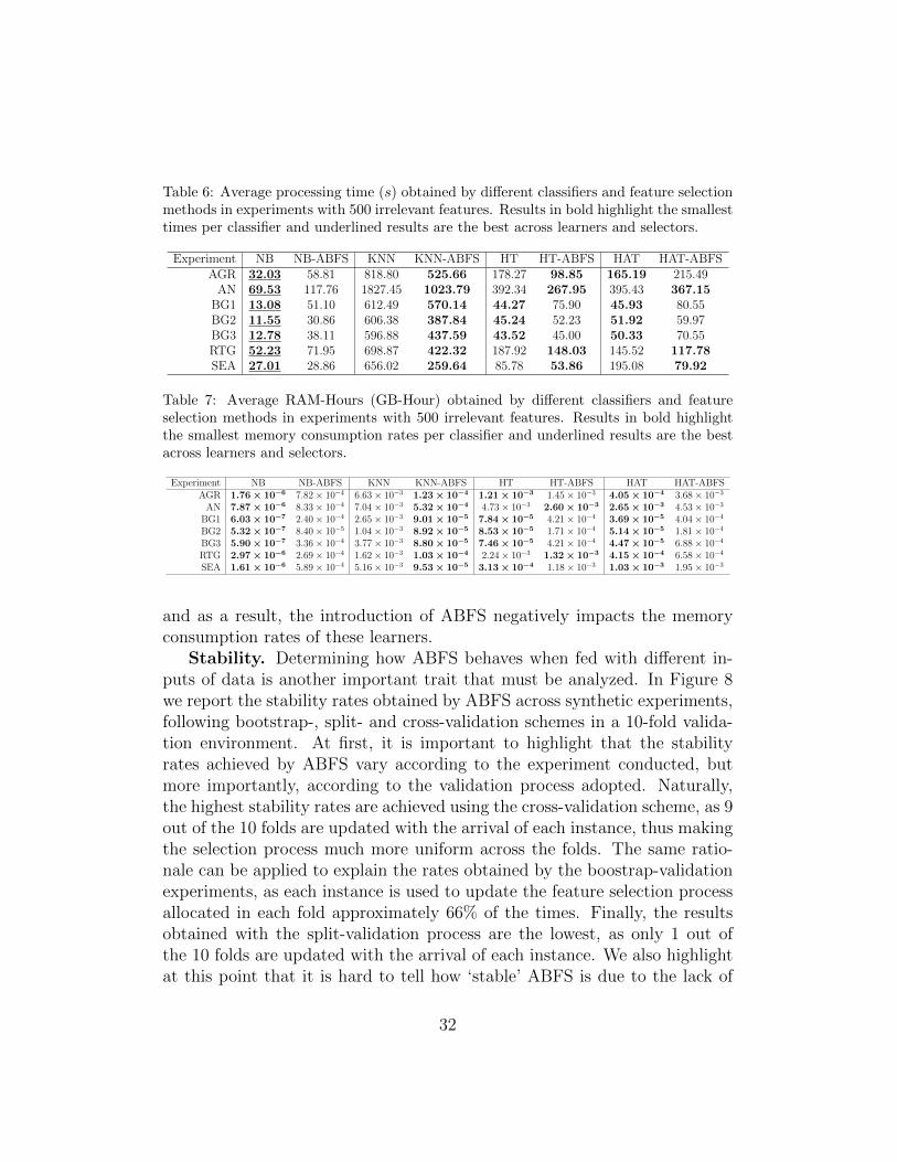
Table 6: Average processing time (s) obtained by different classifiers and feature selectionmethods in experiments with 500 irrelevant features. Results in bold highlight the smallesttimes per classifier and underlined results are the best across learners and selectors.

Experiment NB NB-ABFS KNN KNN-ABFS HT HT-ABFS HAT HAT-ABFSAGR 32.03 58.81 818.80 525.66 178.27 98.85 165.19 215.49

AN 69.53 117.76 1827.45 1023.79 392.34 267.95 395.43 367.15BG1 13.08 51.10 612.49 570.14 44.27 75.90 45.93 80.55BG2 11.55 30.86 606.38 387.84 45.24 52.23 51.92 59.97BG3 12.78 38.11 596.88 437.59 43.52 45.00 50.33 70.55RTG 52.23 71.95 698.87 422.32 187.92 148.03 145.52 117.78SEA 27.01 28.86 656.02 259.64 85.78 53.86 195.08 79.92

Table 7: Average RAM-Hours (GB-Hour) obtained by different classifiers and featureselection methods in experiments with 500 irrelevant features. Results in bold highlightthe smallest memory consumption rates per classifier and underlined results are the bestacross learners and selectors.

Experiment NB NB-ABFS KNN KNN-ABFS HT HT-ABFS HAT HAT-ABFSAGR 1.76 × 10−6 7.82× 10−4 6.63× 10−3 1.23 × 10−4 1.21 × 10−3 1.45× 10−3 4.05 × 10−4 3.68× 10−3

AN 7.87 × 10−6 8.33× 10−4 7.04× 10−3 5.32 × 10−4 4.73× 10−3 2.60 × 10−3 2.65 × 10−3 4.53× 10−3

BG1 6.03 × 10−7 2.40× 10−4 2.65× 10−3 9.01 × 10−5 7.84 × 10−5 4.21× 10−4 3.69 × 10−5 4.04× 10−4

BG2 5.32 × 10−7 8.40× 10−5 1.04× 10−3 8.92 × 10−5 8.53 × 10−5 1.71× 10−4 5.14 × 10−5 1.81× 10−4

BG3 5.90 × 10−7 3.36× 10−4 3.77× 10−3 8.80 × 10−5 7.46 × 10−5 4.21× 10−4 4.47 × 10−5 6.88× 10−4

RTG 2.97 × 10−6 2.69× 10−4 1.62× 10−3 1.03 × 10−4 2.24× 10−3 1.32 × 10−3 4.15 × 10−4 6.58× 10−4

SEA 1.61 × 10−6 5.89× 10−4 5.16× 10−3 9.53 × 10−5 3.13 × 10−4 1.18× 10−3 1.03 × 10−3 1.95× 10−3

and as a result, the introduction of ABFS negatively impacts the memoryconsumption rates of these learners.

Stability. Determining how ABFS behaves when fed with different in-puts of data is another important trait that must be analyzed. In Figure 8we report the stability rates obtained by ABFS across synthetic experiments,following bootstrap-, split- and cross-validation schemes in a 10-fold valida-tion environment. At first, it is important to highlight that the stabilityrates achieved by ABFS vary according to the experiment conducted, butmore importantly, according to the validation process adopted. Naturally,the highest stability rates are achieved using the cross-validation scheme, as 9out of the 10 folds are updated with the arrival of each instance, thus makingthe selection process much more uniform across the folds. The same ratio-nale can be applied to explain the rates obtained by the boostrap-validationexperiments, as each instance is used to update the feature selection processallocated in each fold approximately 66% of the times. Finally, the resultsobtained with the split-validation process are the lowest, as only 1 out ofthe 10 folds are updated with the arrival of each instance. We also highlightat this point that it is hard to tell how ‘stable’ ABFS is due to the lack of

32

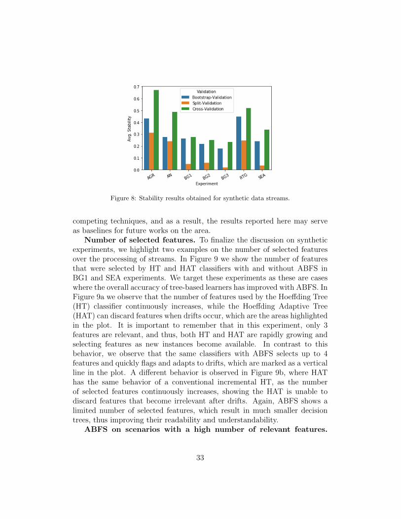
Figure 8: Stability results obtained for synthetic data streams.

competing techniques, and as a result, the results reported here may serveas baselines for future works on the area.

Number of selected features. To finalize the discussion on syntheticexperiments, we highlight two examples on the number of selected featuresover the processing of streams. In Figure 9 we show the number of featuresthat were selected by HT and HAT classifiers with and without ABFS inBG1 and SEA experiments. We target these experiments as these are caseswhere the overall accuracy of tree-based learners has improved with ABFS. InFigure 9a we observe that the number of features used by the Hoeffding Tree(HT) classifier continuously increases, while the Hoeffding Adaptive Tree(HAT) can discard features when drifts occur, which are the areas highlightedin the plot. It is important to remember that in this experiment, only 3features are relevant, and thus, both HT and HAT are rapidly growing andselecting features as new instances become available. In contrast to thisbehavior, we observe that the same classifiers with ABFS selects up to 4features and quickly flags and adapts to drifts, which are marked as a verticalline in the plot. A different behavior is observed in Figure 9b, where HAThas the same behavior of a conventional incremental HT, as the numberof selected features continuously increases, showing the HAT is unable todiscard features that become irrelevant after drifts. Again, ABFS shows alimited number of selected features, which result in much smaller decisiontrees, thus improving their readability and understandability.

ABFS on scenarios with a high number of relevant features.

33

(a) BG1 (b) SEA

Figure 9: Number of features selected and used by decision tree models with and withoutABFS in experiments with 500 irrelevant features. Grayed areas are drifting regions andvertical black lines depict the moments where drifts have been flagged by ABFS. The driftmoments for HT-ABFS and HAT-ABFS match as ABFS is classifier independent.

The experiments conducted and discussed during this section show a smallnumber of relevant features. Therefore, it becomes of interest to determinehow ABFS behaves when confronted with data stream scenarios where arelatively high number of features is required for classification. To achievethis, we conducted a variation of the RTG experiment, where 100 relevantfeatures out of the 500 available are relevant. The results obtained by the 3best-ranked ABFS configurations presented in Figure 6 are reported in Table8, whereas the accuracy rates obtained by classifiers using all the 500 featuresavailable are given in Table 9.

First, it is important to note the selection accuracy rates obtained byABFS, which are competitive with the results obtained in the previous ex-periments, only a smaller number of features was relevant. This, accompaniedby the number of features selected, shows that ABFS is able to scale to sce-narios where more features are required for the classification task. In termsof classification accuracy rates, and comparing the rates shown in Tables 8and 9, we are able to see that ABFS continues to improve NB and KNNlearning schemes, whereas decision trees marginally benefit from the featuresselected by ABFS or even have their accuracy rates prejudiced.

6.3. Real-world datasets

As conducted in the synthetic experiments, the different configurationsof ABFS were ranked across all the real-world experiments according to the

34

Table 8: Results obtained by different configurations of ABFS and base learners in the RTGexperiment with 100 relevant features. Classification accuracy improvements compared tothe results obtained by the same classifier when using all features are reported in bold.

ABFS ConfigurationClassifier Avg. Accuracy (%) Avg. SA Avg. RRF Avg. CUCP Avg. # of features selected

ψ gp θADWIN 500 0.01 NB 64.13%

0.735 0.66 0.91 102ADWIN 500 0.01 KNN 58.58%ADWIN 500 0.01 HT 66.89%ADWIN 500 0.01 HAT 68.11%ADWIN 1000 0.01 NB 62.93%

0.516 0.36 0.88 84ADWIN 1000 0.01 KNN 58.52%ADWIN 1000 0.01 HT 65.49%ADWIN 1000 0.01 HAT 66.61%

HDDM-A 1000 0.01 NB 60.54%

0.569 0.41 0.94 65HDDM-A 1000 0.01 KNN 58.48%HDDM-A 1000 0.01 HT 60.97%HDDM-A 1000 0.01 HAT 62.17%

Table 9: Results obtained by different classifiers in the RTG experiment with 100 relevantfeatures.

Classifier Avg. Accuracy (%)NB 58.46%

KNN 51.83%HT 61.22%

HAT 73.53%

accuracy rates obtained. The 10 best configurations among the 36 tested arereported in Figure 10 with the accuracy results. In contrast to what wasobserved for synthetic experiments, smaller grace periods combined with theADWIN drift detector dominate the top positions, and as a result, we selectgp = 100, θ = 0.05 and ADWIN as the default configuration for real-worldexperiments.

In Table 10 we compare the average accuracy rates obtained by differentclassifiers with and without ABFS across the 30 executions performed. Here,we note that the NB and HT classifiers benefit from ABFS in all experi-ments (at least marginally, as we note in COVTYPE), whereas they matchor improve for KNN. The observed increases are relevant as they broaden1.61% to 19.45% for NB and up to 7.10% for HT. Similarly, the results forHAT show no difference for IADS, while a significant decrease of 4.66% isobserved in NOMAO, another decrease for COVTYPE of 1.86%, and an in-crease of 1.47% for SPAM. Following the outcome of the Wilcoxon test, bothNB and HT classifiers are significantly improved regarding accuracy in thesescenarios, whereas the remainder are not significantly affected.

In Table 11 we compare the processing times of the classifiers with and

35

Table 10: Average accuracy rates (%) obtained by different classifiers and ABFS in real-world experiments. Results in bold are the highest accuracy rates obtained per classifiertype.

Experiment NB ABFS-NB KNN ABFS-KNN HT ABFS-HT HAT ABFS-HATCOVTYPE 70.41 83.20 81.23 84.64 83.77 84.31 82.75 80.89

IADS 80.55 100.00 100.00 100.00 92.90 100.00 82.80 84.00NOMAO 83.36 93.52 94.10 94.43 91.43 94.55 93.67 89.01PAMAP2 97.11 98.72 99.91 99.91 97.66 98.85 86.72 87.91

SPAM 75.78 87.76 86.15 94.14 83.49 88.81 83.45 84.92

without ABFS. Here, we observe similar behavior to what has been observedfor synthetic data, where the processing time rates of all classifiers haveincreased, except for KNN. Here, the Wilcoxon test showed that ABFS sig-nificantly improves the KNN running times, while NB is worsened, and theresults obtained for the remainder of the classifiers are rendered inconclusive.The memory consumption results, depicted in Table 12, show that ABFS alsointroduces overheads to all classifiers. This is a similar behavior to the oneobserved in the previous section, as the actual classification models still allo-cates memory to keep track of statistics about all the original features, eventhough they only update those for the selected ones. One exception worthy

Figure 10: Accuracy rates (%) obtained across the 10-best ranked ABFS configurationsin real-world experiments.

36

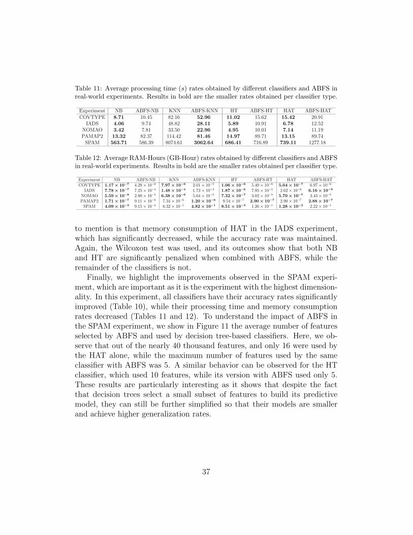
Table 11: Average processing time (s) rates obtained by different classifiers and ABFS inreal-world experiments. Results in bold are the smaller rates obtained per classifier type.

Experiment NB ABFS-NB KNN ABFS-KNN HT ABFS-HT HAT ABFS-HATCOVTYPE 8.71 10.45 82.16 52.96 11.02 15.62 15.42 20.91

IADS 4.06 9.74 48.82 28.11 5.89 10.91 6.78 12.52NOMAO 3.42 7.81 33.50 22.96 4.95 10.01 7.14 11.19PAMAP2 13.32 82.37 114.42 81.46 14.97 89.71 13.15 89.74

SPAM 563.71 586.39 8074.61 3062.64 686.41 716.89 739.11 1277.18

Table 12: Average RAM-Hours (GB-Hour) rates obtained by different classifiers and ABFSin real-world experiments. Results in bold are the smaller rates obtained per classifier type.

Experiment NB ABFS-NB KNN ABFS-KNN HT ABFS-HT HAT ABFS-HATCOVTYPE 1.17 × 10−7 4.29× 10−6 7.97 × 10−6 2.01× 10−5 1.06 × 10−6 5.49× 10−6 5.04 × 10−7 6.97× 10−6

IADS 7.78 × 10−7 7.25× 10−4 1.48 × 10−4 1.73× 10−3 1.87 × 10−6 7.95× 10−4 2.62× 10−6 6.16 × 10−9

NOMAO 5.59 × 10−8 2.80× 10−5 6.38 × 10−6 5.64× 10−5 7.32 × 10−7 3.02× 10−5 5.70 × 10−7 3.43× 10−5

PAMAP2 1.71 × 10−7 9.11× 10−6 7.34× 10−6 1.20 × 10−6 9.54× 10−7 2.90 × 10−7 2.90× 10−7 2.88 × 10−7

SPAM 4.09 × 10−3 9.15× 10−2 6.32× 10−1 4.82 × 10−1 8.51 × 10−3 1.26× 10−1 1.28 × 10−2 2.22× 10−1

to mention is that memory consumption of HAT in the IADS experiment,which has significantly decreased, while the accuracy rate was maintained.Again, the Wilcoxon test was used, and its outcomes show that both NBand HT are significantly penalized when combined with ABFS, while theremainder of the classifiers is not.

Finally, we highlight the improvements observed in the SPAM experi-ment, which are important as it is the experiment with the highest dimension-ality. In this experiment, all classifiers have their accuracy rates significantlyimproved (Table 10), while their processing time and memory consumptionrates decreased (Tables 11 and 12). To understand the impact of ABFS inthe SPAM experiment, we show in Figure 11 the average number of featuresselected by ABFS and used by decision tree-based classifiers. Here, we ob-serve that out of the nearly 40 thousand features, and only 16 were used bythe HAT alone, while the maximum number of features used by the sameclassifier with ABFS was 5. A similar behavior can be observed for the HTclassifier, which used 10 features, while its version with ABFS used only 5.These results are particularly interesting as it shows that despite the factthat decision trees select a small subset of features to build its predictivemodel, they can still be further simplified so that their models are smallerand achieve higher generalization rates.

37

Figure 11: Number of features selected and used during the SPAM experiment.

7. Conclusion

In this paper, we introduced ABFS, an adaptive boosting-based featureselection algorithm for data streams. ABFS includes strategies to selectfeatures over data streams and to detect and adapt to concept drifts. Theproposed method is classifier-independent, and results show that ABFS canimprove all types of classifiers in different scenarios. Despite performinginteresting cuts to the dimensionality of data streams, ABFS still increasesthe processing time and memory consumption of Bayesian and decision tree-based types of learners. An important exception is the KNN classifier, inwhich the results show that both processing times and memory consumptionrates are improved.

In addition to the proposed method, we expect that the contributions onfeature selection evaluation and the framework added to the Massive OnlineAnalysis software to help in the assessment and comparison of future worksin the area. Feature selection-specific metrics, such as Selection Accuracyand Stability have been introduced to streaming scenarios, and the resultsreported here can be assumed as baselines in future works of the area.

As future works, we highlight the following:

• Feature selection based on decision trees and random forests:generally speaking, decision trees can be seen as a feature selectionprocess are they iteratively select features to maximize some ‘purity’metric. Nevertheless, as observed in some of the experiments conductedin this paper, original Hoeffding Trees are prone to overfitting, as theytend to (i) branch over irrelevant features, and (ii) they are unableto prune poor performing branches (except the Hoeffding AdaptiveTree). For instance, the works of [56, 57] are two of many studieswhere only the k-best features used on the first branches of decision

38

trees are used and improve the classification rates of different learners.Also, if the dimensionality of the stream is too big, another importantinvestigation would be to perform feature selection based on AdaptiveRandom Forests [58], as previously conducted on batch scenarios onthe works of [59, 60].

• Distributed feature selection: feature selection and dimensionalityreduction are of the utmost importance when the number of features ina data stream grows up to thousands or millions. Therefore, proposingfeature selection techniques that can be paralleled and scaled up tothese extreme scenarios is another important gap to be pursued.

• Feature selection on semi-supervised, unsupervised and de-layed labelling learning schemes: in real-world scenarios the as-sumption that all instances are labeled is unlikely to hold. Thus, itis important to tailor feature selection techniques that can accuratelyselect features with very few or even no labels at all (for clustering sce-narios). Closely related to this topic, feature selection methods shouldalso be able to handle delayed labelling scenarios, where the labels ofinstances become available, but after a delay of n instances.

Acknowledgments

This project was financially supported by the Coordenacao de Aper-feicoamento de Pessoal de Nıvel Superior (CAPES) through the Programade Suporte a Pos-Graduacao de Instituicoes de Ensino Particulares (PRO-SUP) program for Doctorate students. Part of this research has also beenconducted with a grant for visiting researchers also provided by CAPES un-der grant number 88881.131817/2016-01. Finally, we truthfully thank thereviewers for the constructive comments that yielded relevant changes in ourinitial manuscript and how the assessment of the methods was done.

References

[1] A. L. Blum, P. Langley, Selection of relevant features and exam-ples in machine learning, Artif. Intell. 97 (1-2) (1997) 245–271.doi:10.1016/S0004-3702(97)00063-5.URL http://dx.doi.org/10.1016/S0004-3702(97)00063-5

39

[2] D. W. Opitz, Feature selection for ensembles, in: Proceedings of theSixteenth National Conference on Artificial Intelligence and the EleventhInnovative Applications of Artificial Intelligence Conference InnovativeApplications of Artificial Intelligence, AAAI ’99/IAAI ’99, AmericanAssociation for Artificial Intelligence, Menlo Park, CA, USA, 1999, pp.379–384.URL http://dl.acm.org/citation.cfm?id=315149.315328

[3] Y. Yang, J. O. Pedersen, A comparative study on feature selectionin text categorization, in: Proceedings of the Fourteenth InternationalConference on Machine Learning, ICML ’97, Morgan Kaufmann Pub-lishers Inc., San Francisco, CA, USA, 1997, pp. 412–420.URL http://dl.acm.org/citation.cfm?id=645526.657137

[4] M. L. Bermingham, R. Pong-Wong, A. Spiliopoulou, C. Hayward,I. Rudan, H. Campbell, A. F. Wright, J. F. Wilson, F. Agakov,P. Navarro, C. S. Haley, Application of high-dimensional feature se-lection: evaluation for genomic prediction in man, Scientific Reports 5.URL http://dx.doi.org/10.1038/srep10312

[5] G. Widmer, M. Kubat, Learning in the presence of conceptdrift and hidden contexts, Mach. Learn. 23 (1) (1996) 69–101.doi:10.1023/A:1018046501280.

[6] N. Oza, Online bagging and boosting, in: Systems, Man and Cybernet-ics, 2005 IEEE International Conference on, Vol. 3, 2005, pp. 2340–2345Vol. 3. doi:10.1109/ICSMC.2005.1571498.

[7] A. Bifet, G. Holmes, R. Kirkby, B. Pfahringer, MOA: Massive onlineanalysis, The Journal of Machine Learning Research 11 (2010) 1601–1604.

[8] J. P. Barddal, H. M. Gomes, F. Enembreck, B. Pfahringer, A. Bifet,On dynamic feature weighting for feature drifting data streams, in:ECML/PKDD’16, Lecture Notes in Computer Science, Springer, 2016.

[9] P.-N. Tan, M. Steinbach, V. Kumar, Introduction to Data Mining, (Sec-ond Edition), Addison-Wesley Longman Publishing Co., Inc., Boston,MA, USA, 2006.

40

[10] Z. Zhao, F. Morstatter, S. Sharma, S. Alelyani, A. Anand, H. Liu,Advancing feature selection research, ASU feature selection repository(2010) 1–28.

[11] G. Chandrashekar, F. Sahin, A survey on feature se-lection methods, Computers & Electrical Engineering40 (1) (2014) 16 – 28, 40th-year commemorative issue.doi:http://dx.doi.org/10.1016/j.compeleceng.2013.11.024.URL http://www.sciencedirect.com/science/article/pii/

S0045790613003066

[12] H.-L. Nguyen, Y.-K. Woon, W.-K. Ng, L. Wan, Heterogeneous ensem-ble for feature drifts in data streams, in: P.-N. Tan, S. Chawla, C. Ho,J. Bailey (Eds.), Advances in Knowledge Discovery and Data Mining,Vol. 7302 of Lecture Notes in Computer Science, Springer Berlin Hei-delberg, 2012, pp. 1–12. doi:10.1007/978-3-642-30220-6 1.URL http://dx.doi.org/10.1007/978-3-642-30220-6\_1

[13] S. C. H. Hoi, J. Wang, P. Zhao, R. Jin, Online feature selection formining big data, in: Proceedings of the 1st International Workshopon Big Data, Streams and Heterogeneous Source Mining: Algorithms,Systems, Programming Models and Applications, BigMine ’12, ACM,New York, NY, USA, 2012, pp. 93–100. doi:10.1145/2351316.2351329.URL http://doi.acm.org/10.1145/2351316.2351329

[14] J. Wang, P. Zhao, S. C. H. Hoi, R. Jin, Online feature selection and itsapplications, IEEE Transactions on Knowledge and Data Engineering26 (3) (2014) 698–710. doi:10.1109/TKDE.2013.32.

[15] D. Zhou, J. Huang, B. Scholkopf, Learning from labeled and unlabeleddata on a directed graph, in: Machine Learning, Proceedings of theTwenty-Second International Conference (ICML 2005), Bonn, Germany,August 7-11, 2005, 2005, pp. 1036–1043. doi:10.1145/1102351.1102482.URL http://doi.acm.org/10.1145/1102351.1102482

[16] J. P. Barddal, H. M. Gomes, A. de Souza Britto Jr., F. Enembreck, Abenchmark of classifiers on feature drifting data streams, in: ICPR’16,Lecture Notes in Computer Science, Springer, 2016.

41

[17] J. P. Barddal, H. M. Gomes, F. Enembreck, B. Pfahringer, A surveyon feature drift adaptation: Definition, benchmark, challenges and fu-ture directions, Journal of Systems and Software 127 (2017) 278 – 294.doi:https://doi.org/10.1016/j.jss.2016.07.005.

[18] P. Domingos, G. Hulten, Mining high-speed data streams, in: Proceed-ings of the Sixth ACM SIGKDD International Conference on KnowledgeDiscovery and Data Mining, KDD ’00, ACM, New York, NY, USA, 2000,pp. 71–80. doi:10.1145/347090.347107.URL http://doi.acm.org/10.1145/347090.347107

[19] A. Bifet, R. Gavalda, Adaptive Learning from Evolving Data Streams,Springer Berlin Heidelberg, Berlin, Heidelberg, 2009, pp. 249–260.doi:10.1007/978-3-642-03915-7 22.

[20] A. Bifet, R. Gavalda, Learning from time-changing data with adaptivewindowing, in: In SIAM International Conference on Data Mining, 2007.

[21] I. H. Witten, E. Frank, Data Mining: Practical Machine Learning Toolsand Techniques, Second Edition (Morgan Kaufmann Series in DataManagement Systems), Morgan Kaufmann Publishers Inc., San Fran-cisco, CA, USA, 2005.

[22] H. Huang, S. Yoo, S. P. Kasiviswanathan, Unsupervised feature se-lection on data streams, in: Proceedings of the 24th ACM In-ternational on Conference on Information and Knowledge Manage-ment, CIKM ’15, ACM, New York, NY, USA, 2015, pp. 1031–1040.doi:10.1145/2806416.2806521.

[23] J. Duarte, J. Gama, Feature ranking in hoeffding algorithms for re-gression, in: Proceedings of the Symposium on Applied Comput-ing, SAC ’17, ACM, New York, NY, USA, 2017, pp. 836–841.doi:10.1145/3019612.3019670.URL http://doi.acm.org/10.1145/3019612.3019670

[24] J. A. Silva, E. R. Faria, R. C. Barros, E. R. Hruschka, A. C. P. L. F. d.Carvalho, J. Gama, Data stream clustering: A survey, ACM Comput.Surv. 46 (1) (2013) 13:1–13:31. doi:10.1145/2522968.2522981.

42

[25] R. E. Schapire, The strength of weak learnability, Mach. Learn. 5 (2)(1990) 197–227. doi:10.1023/A:1022648800760.URL https://doi.org/10.1023/A:1022648800760

[26] R. Appel, P. Perona, A simple multi-class boosting framework with the-oretical guarantees and empirical proficiency, in: D. Precup, Y. W. Teh(Eds.), Proceedings of the 34th International Conference on MachineLearning, Vol. 70 of Proceedings of Machine Learning Research, PMLR,International Convention Centre, Sydney, Australia, 2017, pp. 186–194.URL http://proceedings.mlr.press/v70/appel17a.html

[27] Q. Miao, Y. Cao, G. Xia, M. Gong, J. Liu, J. Song, Rboost: La-bel noise-robust boosting algorithm based on a nonconvex loss func-tion and the numerically stable base learners, IEEE Transactions onNeural Networks and Learning Systems 27 (11) (2016) 2216–2228.doi:10.1109/TNNLS.2015.2475750.

[28] R. E. Schapire, A brief introduction to boosting, in: Proceedings of the16th International Joint Conference on Artificial Intelligence - Volume 2,IJCAI’99, Morgan Kaufmann Publishers Inc., San Francisco, CA, USA,1999, pp. 1401–1406.URL http://dl.acm.org/citation.cfm?id=1624312.1624417

[29] R. Pelossof, M. Jones, I. Vovsha, C. Rudin, Online coordinateboosting, in: 2009 IEEE 12th International Conference on Com-puter Vision Workshops, ICCV Workshops, 2009, pp. 1354–1361.doi:10.1109/ICCVW.2009.5457454.

[30] B. Wang, J. Pineau, Online bagging and boosting for imbalanced datastreams, IEEE Transactions on Knowledge and Data Engineering 28 (12)(2016) 3353–3366. doi:10.1109/TKDE.2016.2609424.

[31] H. Hu, W. Sun, A. Venkatraman, M. Hebert, J. A. Bagnell, Gra-dient boosting on stochastic data streams, CoRR abs/1703.00377.arXiv:1703.00377.URL http://arxiv.org/abs/1703.00377

[32] Z. Xu, G. Huang, K. Q. Weinberger, A. X. Zheng, Gradient boosted fea-ture selection, in: Proceedings of the 20th ACM SIGKDD InternationalConference on Knowledge Discovery and Data Mining, KDD ’14, ACM,

43

New York, NY, USA, 2014, pp. 522–531. doi:10.1145/2623330.2623635.URL http://doi.acm.org/10.1145/2623330.2623635

[33] S. Das, Filters, wrappers and a boosting-based hybrid for feature se-lection, in: Proceedings of the Eighteenth International Conference onMachine Learning, ICML ’01, Morgan Kaufmann Publishers Inc., SanFrancisco, CA, USA, 2001, pp. 74–81.URL http://dl.acm.org/citation.cfm?id=645530.658297

[34] Q. Miao, Y. Cao, J. Song, J. Liu, Y. Quan, Boostfs: Aboosting-based irrelevant feature selection algorithm, IJPRAI 29 (7).doi:10.1142/S0218001415510118.URL http://dx.doi.org/10.1142/S0218001415510118

[35] W. Hoeffding, Probability inequalities for sums of bounded random vari-ables, Journal of the American Statistical Association 58 (301) (1963)13–30.URL http://www.jstor.org/stable/2282952?

[36] I. Frıas-Blanco, J. d. Campo-Avila, G. Ramos-Jimenez, R. Morales-Bueno, A. Ortiz-Diaz, Y. Caballero-Mota, Online and non-parametricdrift detection methods based on hoeffding bounds, IEEE Transac-tions on Knowledge and Data Engineering 27 (3) (2015) 810–823.doi:10.1109/TKDE.2014.2345382.

[37] S. Galelli, G. B. Humphrey, H. R. Maier, A. Castelletti,G. C. Dandy, M. S. Gibbs, An evaluation framework for inputvariable selection algorithms for environmental data-driven mod-els, Environmental Modelling & Software 62 (2014) 33 – 51.doi:http://dx.doi.org/10.1016/j.envsoft.2014.08.015.

[38] J. Gama, P. Rodrigues, Issues in evaluation of stream learning algo-rithms, in: Proc. of the 15th ACM SIGKDD international conferenceon Knowledge discovery and data mining, ACM SIGKDD, 2009, pp.329–338.

[39] L. Molina, L. Belanche, A. Nebot, Feature selection algorithms: a sur-vey and experimental evaluation, in: Data Mining, 2002. ICDM 2003.Proceedings. 2002 IEEE International Conference on, 2002, pp. 306–313.doi:10.1109/ICDM.2002.1183917.

44

[40] L. I. Kuncheva, A stability index for feature selection, in: Proceed-ings of the 25th Conference on Proceedings of the 25th IASTED In-ternational Multi-Conference: Artificial Intelligence and Applications,AIAP’07, ACTA Press, Anaheim, CA, USA, 2007, pp. 390–395.URL http://dl.acm.org/citation.cfm?id=1295303.1295370

[41] S. Nogueira, G. Brown, Measuring the stability of feature selection, in:Machine Learning and Knowledge Discovery in Databases - EuropeanConference, ECML PKDD 2016, Riva del Garda, Italy, September 19-23,2016, Proceedings, Part II, 2016, pp. 442–457. doi:10.1007/978-3-319-46227-1 28.

[42] A. Bifet, G. de Francisci Morales, J. Read, G. Holmes, B. Pfahringer,Efficient online evaluation of big data stream classifiers, in: Proceedingsof the 21th ACM SIGKDD International Conference on Knowledge Dis-covery and Data Mining, KDD ’15, ACM, New York, NY, USA, 2015,pp. 59–68. doi:10.1145/2783258.2783372.URL http://doi.acm.org/10.1145/2783258.2783372

[43] R. Agrawal, T. Imielinski, A. Swami, Database mining: a performanceperspective, Knowledge and Data Engineering, IEEE Transactions on5 (6) (1993) 914–925. doi:10.1109/69.250074.

[44] F. Enembreck, B. C. Avila, E. E. Scalabrin, J.-P. A. Barthes, Learningdrifting negotiations., Applied Artificial Intelligence 21 (9) (2007)861–881.URL http://dblp.uni-trier.de/db/journals/aai/aai21.html#

EnembreckASB07

[45] M. A. Hall, Correlation-based feature selection for discrete and numericclass machine learning, in: Proceedings of the Seventeenth InternationalConference on Machine Learning, ICML ’00, Morgan Kaufmann Pub-lishers Inc., San Francisco, CA, USA, 2000, pp. 359–366.URL http://dl.acm.org/citation.cfm?id=645529.657793

[46] W. N. Street, Y. Kim, A streaming ensemble algorithm (sea) for large-classification, in: Proc. of the seventh ACM SIGKDD international con-ference on Knowledge discovery and data mining, ACM SIGKDD, 2001,pp. 377–382.

45

[47] J. A. Blackard, D. J. Dean, Comparative accuracies of artificial neuralnetworks and discriminant analysis in predicting forest cover types fromcartographic variables, Computers and Electronics in Agriculture 24 (3)(1999) 131 – 151. doi:https://doi.org/10.1016/S0168-1699(99)00046-0.URL http://www.sciencedirect.com/science/article/pii/

S0168169999000460

[48] N. Kushmerick, Learning to remove internet advertisements, in: Pro-ceedings of the third annual conference on Autonomous Agents, ACM,1999, pp. 175–181.

[49] L. Candillier, V. Lemaire, Design and analysis of the nomao challengeactive learning in the real-world, in: Proceedings of the ALRA: ActiveLearning in Real-world Applications, Workshop ECML-PKDD, 2012.

[50] A. Reiss, D. Stricker, Introducing a new benchmarked dataset foractivity monitoring, in: Proceedings of the 2012 16th Annual In-ternational Symposium on Wearable Computers (ISWC), ISWC ’12,IEEE Computer Society, Washington, DC, USA, 2012, pp. 108–109.doi:10.1109/ISWC.2012.13.URL https://doi.org/10.1109/ISWC.2012.13

[51] I. Katakis, G. Tsoumakas, I. Vlahavas, Dynamic feature space and incre-mental feature selection for the classification of textual data streams, in:in ECML/PKDD-2006 International Workshop on Knowledge Discoveryfrom Data Streams. 2006, Springer Verlag, 2006, p. 107.

[52] F. Wilcoxon, Individual Comparisons by Ranking Methods, BiometricsBulletin 1 (6) (1945) 80–83. doi:10.2307/3001968.URL http://dx.doi.org/10.2307/3001968

[53] M. Friedman, The Use of Ranks to Avoid the Assumption of NormalityImplicit in the Analysis of Variance, Journal of the American StatisticalAssociation 32 (200) (1937) 675–701. doi:10.2307/2279372.URL http://dx.doi.org/10.2307/2279372

[54] P. Nemenyi, Distribution-free multiple comparisons, Ph.D. thesis, NewJersey, USA (1963).

46

[55] J. Demsar, Statistical comparisons of classifiers over multiple data sets,J. Mach. Learn. Res. 7 (2006) 1–30.URL http://dl.acm.org/citation.cfm?id=1248547.1248548

[56] V. Sugumaran, V. Muralidharan, K. Ramachandran, Feature se-lection using decision tree and classification through proximalsupport vector machine for fault diagnostics of roller bearing, Me-chanical Systems and Signal Processing 21 (2) (2007) 930 – 942.doi:https://doi.org/10.1016/j.ymssp.2006.05.004.URL http://www.sciencedirect.com/science/article/pii/

S0888327006001142

[57] N. M. Tahir, A. Hussain, S. A. Samad, K. A. Ishak, R. A. Halim,Feature selection for classification using decision tree, in: 2006 4thStudent Conference on Research and Development, 2006, pp. 99–102.doi:10.1109/SCORED.2006.4339317.

[58] H. M. Gomes, A. Bifet, J. Read, J. P. Barddal, F. Enembreck,B. Pfharinger, G. Holmes, T. Abdessalem, Adaptive random forests forevolving data stream classification, Machine Learning 106 (9) (2017)1469–1495. doi:10.1007/s10994-017-5642-8.URL https://doi.org/10.1007/s10994-017-5642-8

[59] A. P. Cassidy, F. A. Deviney, Calculating feature importance in datastreams with concept drift using online random forest, in: 2014 IEEEInternational Conference on Big Data (Big Data), 2014, pp. 23–28.doi:10.1109/BigData.2014.7004352.

[60] A. Verikas, A. Gelzinis, M. Bacauskiene, Mining data with randomforests: A survey and results of new tests, Pattern Recognition 44 (2)(2011) 330–349.

47

View publication statsView publication stats

https://www.researchgate.net/publication/331047437

boosting decision stumps for dynamic feature selection on

Documents