boosting efficiency for computing the pareto frontier on
TRANSCRIPT
Boosting Efficiency for Computingthe Pareto Frontier on Tree Structured
Networks
Jonathan M. Gomes-Selman1, Qinru Shi2, Yexiang Xue3,Roosevelt Garcıa-Villacorta4, Alexander S. Flecker4, and Carla P. Gomes3(B)
1 Department of Computer Science, Stanford University, Stanford, [email protected]
2 Center for Applied Mathematics, Cornell University, Ithaca, [email protected]
3 Department of Computer Science, Cornell University, Ithaca, [email protected], [email protected]
4 Department of Ecology and Evolutionary Biology, Cornell University, Ithaca, [email protected], [email protected]
Abstract. Multi-objective optimization plays a key role in the studyof real-world problems, as they often involve multiple criteria. In multi-objective optimization it is important to identify the so-called Paretofrontier, which characterizes the trade-offs between the objectives of dif-ferent solutions. We show how a divide-and-conquer approach, combinedwith batched processing and pruning, significantly boosts the perfor-mance of an exact and approximation dynamic programming (DP) algo-rithm for computing the Pareto frontier on tree-structured networks, pro-posed in [18]. We also show how exploiting restarts and a new instanceselection strategy boosts the performance and accuracy of a mixed inte-ger programming (MIP) approach for approximating the Pareto fron-tier. We provide empirical results demonstrating that our DP and MIPapproaches have complementary strengths and outperform previous algo-rithms in efficiency and accuracy. Our work is motivated by a problemin computational sustainability concerning the evaluation of trade-offs inecosystem services due to the proliferation of hydropower dams through-out the Amazon basin. Our approaches are general and can be appliedto computing the Pareto frontier of a variety of multi-objective problemson tree-structured networks.
Keywords: Multi-objective optimization · Pareto frontierApproximation algorithms · Dynamic programmingMixed-integer programming
J.M. Gomes-Selman and Q. Shi—These authors are contributed Equally.
c© Springer International Publishing AG, part of Springer Nature 2018W.-J. van Hoeve (Ed.): CPAIOR 2018, LNCS 10848, pp. 263–279, 2018.https://doi.org/10.1007/978-3-319-93031-2_19
264 J. M. Gomes-Selman et al.
1 Introduction
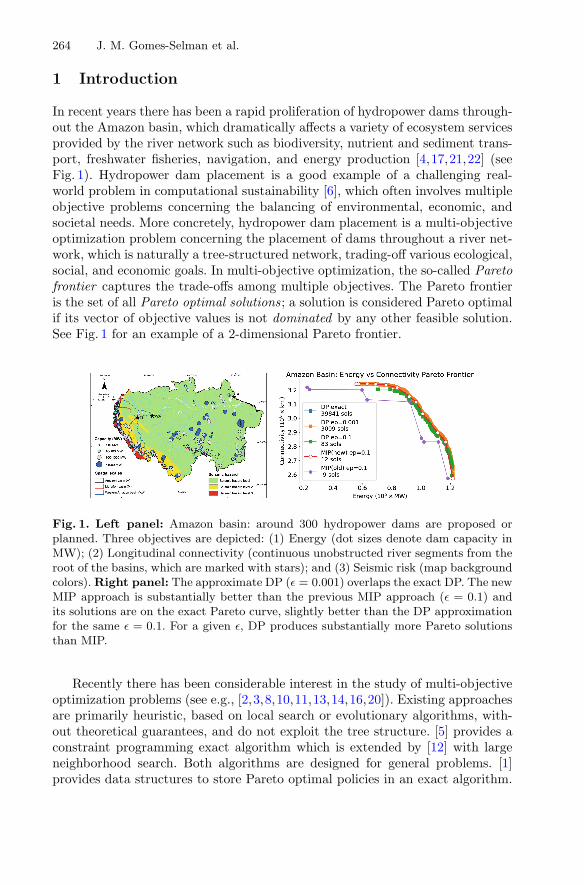
In recent years there has been a rapid proliferation of hydropower dams through-out the Amazon basin, which dramatically affects a variety of ecosystem servicesprovided by the river network such as biodiversity, nutrient and sediment trans-port, freshwater fisheries, navigation, and energy production [4,17,21,22] (seeFig. 1). Hydropower dam placement is a good example of a challenging real-world problem in computational sustainability [6], which often involves multipleobjective problems concerning the balancing of environmental, economic, andsocietal needs. More concretely, hydropower dam placement is a multi-objectiveoptimization problem concerning the placement of dams throughout a river net-work, which is naturally a tree-structured network, trading-off various ecological,social, and economic goals. In multi-objective optimization, the so-called Paretofrontier captures the trade-offs among multiple objectives. The Pareto frontieris the set of all Pareto optimal solutions; a solution is considered Pareto optimalif its vector of objective values is not dominated by any other feasible solution.See Fig. 1 for an example of a 2-dimensional Pareto frontier.
Fig. 1. Left panel: Amazon basin: around 300 hydropower dams are proposed orplanned. Three objectives are depicted: (1) Energy (dot sizes denote dam capacity inMW); (2) Longitudinal connectivity (continuous unobstructed river segments from theroot of the basins, which are marked with stars); and (3) Seismic risk (map backgroundcolors). Right panel: The approximate DP (ε = 0.001) overlaps the exact DP. The newMIP approach is substantially better than the previous MIP approach (ε = 0.1) andits solutions are on the exact Pareto curve, slightly better than the DP approximationfor the same ε = 0.1. For a given ε, DP produces substantially more Pareto solutionsthan MIP.
Recently there has been considerable interest in the study of multi-objectiveoptimization problems (see e.g., [2,3,8,10,11,13,14,16,20]). Existing approachesare primarily heuristic, based on local search or evolutionary algorithms, with-out theoretical guarantees, and do not exploit the tree structure. [5] provides aconstraint programming exact algorithm which is extended by [12] with largeneighborhood search. Both algorithms are designed for general problems. [1]provides data structures to store Pareto optimal policies in an exact algorithm.
Boosting Efficiency for Computing the Pareto Frontier 265
This paper focuses on computing the Pareto frontier, both exact and with approx-imation guarantees, on tree-structured networks. In [18] we proposed a dynamicprogramming algorithm for trees which computes the exact Pareto frontier, aswell as a rounding technique applied to the exact dynamic programming algo-rithm that provides a fully polynomial-time approximation scheme (FPTAS).The FPTAS finds a solution set of polynomial size, which approximates thePareto frontier within an arbitrary small ε factor and runs in time that is poly-nomial in the size of the instance and 1/ε. We also formulated the problemof optimizing the placement of dams as a mixed integer programming problem(MIP) and used it to approximate the Pareto frontier. While the results in [18]are encouraging, there is room for improvement.
Our Contributions: (1) A key component of our DP algorithm is the prun-ing of dominated solutions. We provide a divide-and-conquer approach thatsignificantly improves the efficiency of the pruning of dominated solu-tions and outperforms the previous approach, leading to speed-ups of twoto three orders of magnitude, in practice; (2) To cope with the large mem-ory requirements of a multi-objective Pareto frontier, we propose batching toidentify and prune dominated solutions incrementally, scaling up tomuch larger problems; (3) We also propose a new MIP based approxima-tion scheme that exploits restarts and a new instance selection strategy, whichboosts the performance and accuracy of the previous MIP approach for approx-imating the Pareto frontier. (4) We design a visualization tool of our resultsintended for decision makers. (5) We provide empirical results showing that ourproposed algorithms significantly outperform previous approaches.
Preview of Results: Our DP and MIP Pareto frontier algorithms are com-plementary and scale up to much larger real-world instances than previous algo-rithms: the DP can now approximate the Pareto frontier for the entireAmazon basin, when optimizing for energy, connectivity (a proxy for e.g.,unimpeded fish migrations and transportation), seismic risk, and sediment, inaround 5 days, with a coverage of 2, 193, 314 non-dominated solutions, withthe guarantee that the solutions are within at most 5% of the true optimum(ε = 0.05); in less than 6 h, the DP provides a coverage of 491, 578 non-dominatedsolutions (ε = 0.1); in around 6.5 min, the DP provides a coverage of 23, 019non-dominated solutions (ε = 0.25); for the same ε = 0.25, the MIP approachapproximates the Pareto frontier in around 25 min, with a smaller coverage of95 non-dominated solutions, but the MIP approach provides more flexibilitywhen considering additional constraints and, in practice, its solutions tend tobe closer to the exact Pareto frontier for a given ε. Our overall goal is to enablemore informed decisions concerning the trade-offs of multiple objectives of opti-mization problems.
266 J. M. Gomes-Selman et al.
2 Problem Formulation
In this section, we first introduce the hydropower dam placement problem as anexample of a multi-objective optimization problem on a tree structured network.Then, we show the general formulation of such problems.
(a) River Network (b) Directed RootedTree
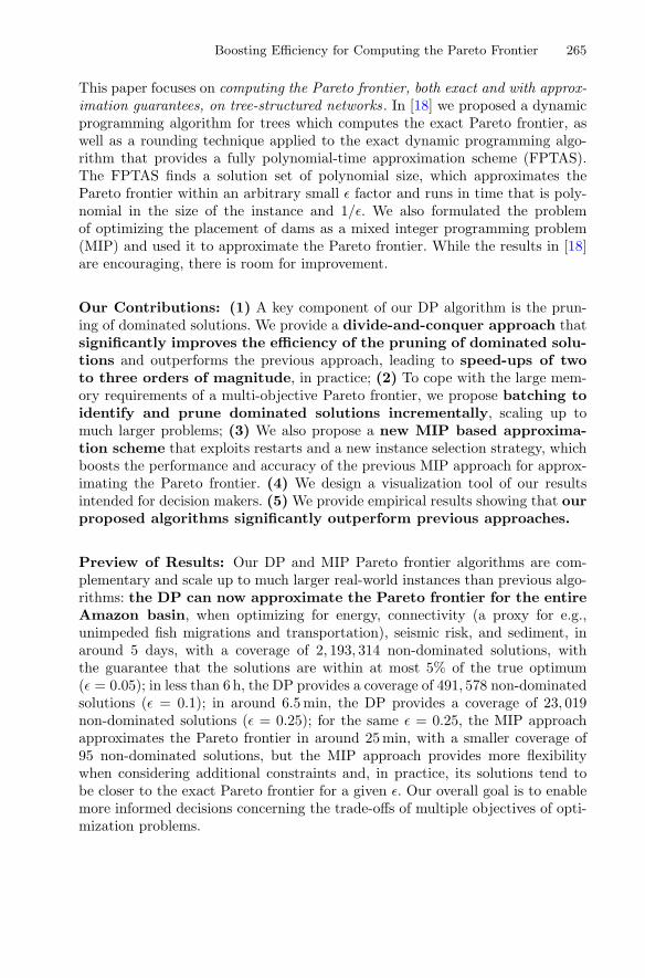
Fig. 2. Converting a river network (left) into a more compact directed rooted tree(right: x is the root). Each contiguous region of the river network (represented bydifferent colors, and labeled x, u, v, w) is converted into a node, also referred to as ahypernode (labeled with the corresponding letter, x, u, v, w) in the tree network. Eachpotential dam site (represented by a red-yellow circle) is represented by an edge in thedirected rooted tree. (Color figure online)
2.1 Hydropower Dam Placement Problem
We are given a set of planned dams and need to decide the optimal subsetof dams to build. We refer to this problem as the hydropower dam placementproblem. We first point out that a river network is a directed tree-structurenetwork and that, for the purposes of our hydropower dam placement problem,we don’t need to explicitly consider every river segment. So, we first abstract theriver network and potential dam locations into a more compact directed rootedtree that captures the key problem information. Each contiguous section of theriver network uninterrupted by existing or potential dam locations is representedby a node (we also call it hypernode to emphasize that it encapsulates a river subnetwork). Each existing or potential dam location is represented by a directededge pointing from downstream to upstream. See Fig. 2 for an example of ourconversion of a river network into a more compact directed rooted tree.
A policy (or solution) π is a subset of potential dam sites to be built. Wecan encode many environmental and economical objectives as a function of π.In this paper, we focus on the following four objectives:
Energy (E): Given a solution π, the total hydropower produced by the selecteddams is E(π) =
∑e∈π he, where he is the hydropower of the dam represented
by edge e. We want to maximize this objective.
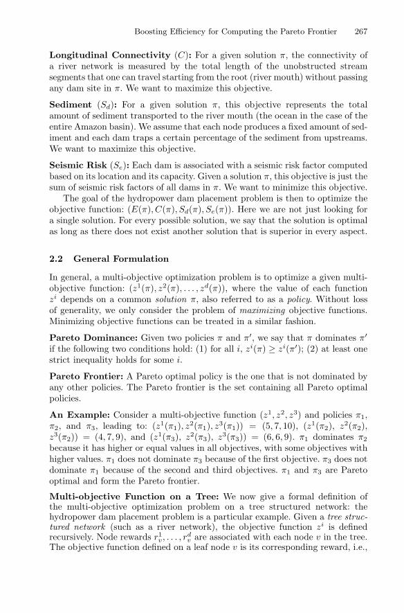
Boosting Efficiency for Computing the Pareto Frontier 267
Longitudinal Connectivity (C): For a given solution π, the connectivity ofa river network is measured by the total length of the unobstructed streamsegments that one can travel starting from the root (river mouth) without passingany dam site in π. We want to maximize this objective.
Sediment (Sd): For a given solution π, this objective represents the totalamount of sediment transported to the river mouth (the ocean in the case of theentire Amazon basin). We assume that each node produces a fixed amount of sed-iment and each dam traps a certain percentage of the sediment from upstreams.We want to maximize this objective.
Seismic Risk (Se): Each dam is associated with a seismic risk factor computedbased on its location and its capacity. Given a solution π, this objective is just thesum of seismic risk factors of all dams in π. We want to minimize this objective.
The goal of the hydropower dam placement problem is then to optimize theobjective function: (E(π), C(π), Sd(π), Se(π)). Here we are not just looking fora single solution. For every possible solution, we say that the solution is optimalas long as there does not exist another solution that is superior in every aspect.
2.2 General Formulation
In general, a multi-objective optimization problem is to optimize a given multi-objective function: (z1(π), z2(π), . . . , zd(π)), where the value of each functionzi depends on a common solution π, also referred to as a policy. Without lossof generality, we only consider the problem of maximizing objective functions.Minimizing objective functions can be treated in a similar fashion.
Pareto Dominance: Given two policies π and π′, we say that π dominates π′
if the following two conditions hold: (1) for all i, zi(π) ≥ zi(π′); (2) at least onestrict inequality holds for some i.
Pareto Frontier: A Pareto optimal policy is the one that is not dominated byany other policies. The Pareto frontier is the set containing all Pareto optimalpolicies.
An Example: Consider a multi-objective function (z1, z2, z3) and policies π1,π2, and π3, leading to: (z1(π1), z2(π1), z3(π1)) = (5, 7, 10), (z1(π2), z2(π2),z3(π2)) = (4, 7, 9), and (z1(π3), z2(π3), z3(π3)) = (6, 6, 9). π1 dominates π2
because it has higher or equal values in all objectives, with some objectives withhigher values. π1 does not dominate π3 because of the first objective. π3 does notdominate π1 because of the second and third objectives. π1 and π3 are Paretooptimal and form the Pareto frontier.
Multi-objective Function on a Tree: We now give a formal definition ofthe multi-objective optimization problem on a tree structured network: thehydropower dam placement problem is a particular example. Given a tree struc-tured network (such as a river network), the objective function zi is definedrecursively. Node rewards r1v, . . . , rd
v are associated with each node v in the tree.The objective function defined on a leaf node v is its corresponding reward, i.e.,
268 J. M. Gomes-Selman et al.
ziv(π) = ri
v. Each edge is associated with a transfer coefficient that is affected bywhether the corresponding dam is built or not. If the dam represented by (u, v) isbuilt, then (u, v) has a transfer coefficient of pi
uv; otherwise, qiuv. Also associated
with each edge (u, v) is a reward siuv and an indicator variable denoting whether
the corresponding edge is in π or not. The objective function on a non-leaf nodeu is defined recursively:
ziu(π) = riu +
∑
v∈ch(u)
I(uv ∈ π)siuv +∑
v∈ch(u)
(I(uv ∈ π)pi
uv + I(uv /∈ π)qiuv
)ziv(π). (1)
Here, I(·) is an indicator function. ch(u) is the child set of u. The objectivefunction for the entire tree network T is the function at the root node s, i.e.,zi(π) = zi
s(π). Given a multi-objective function defined on a tree network T , ourmulti-objective optimization problem on a tree structured networkis to find the Pareto frontier consisting of all non-dominated policies, which isNP-hard even though it is defined on a tree. See [18] for further details.
Application to the Hydropower Dam Placement Problem: In thehydropower dam placement problem, when modeling connectivity (i.e., i =connectivity), we set ri
u to be the total lengths of all stream segments in theregion represented by node u. We set pi
uv = 0 and qiuv = 1; that is, we either
acquire all upstream segments (when the dam corresponding to edge (u, v) is notbuilt) or lose all of them (when the dam is built). We set si
uv = 0. When model-ing energy (i.e., i = energy), we set si
uv = huv, in which huv is the hydropowerproduced by the dam site (u, v). ri
u is set to 0, piuv and qi
uv are both set to 1.
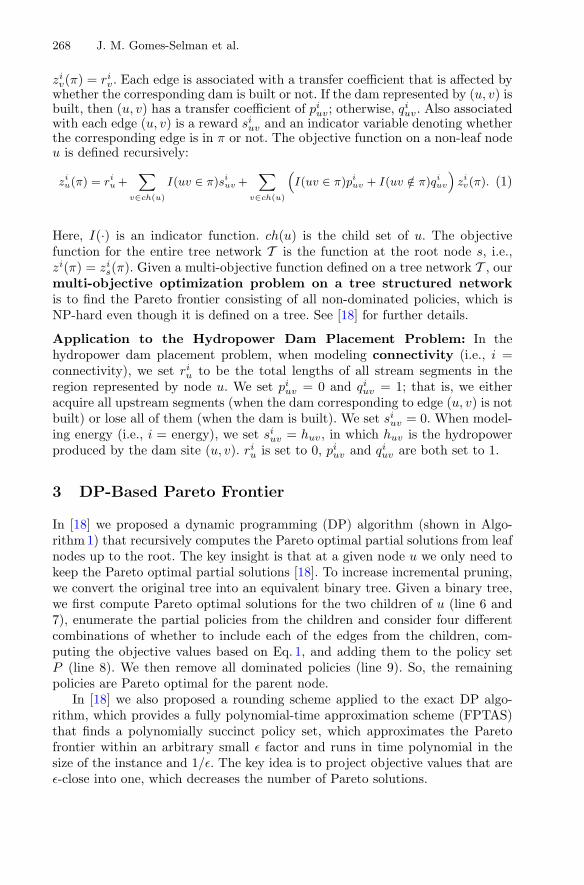
3 DP-Based Pareto Frontier
In [18] we proposed a dynamic programming (DP) algorithm (shown in Algo-rithm1) that recursively computes the Pareto optimal partial solutions from leafnodes up to the root. The key insight is that at a given node u we only need tokeep the Pareto optimal partial solutions [18]. To increase incremental pruning,we convert the original tree into an equivalent binary tree. Given a binary tree,we first compute Pareto optimal solutions for the two children of u (line 6 and7), enumerate the partial policies from the children and consider four differentcombinations of whether to include each of the edges from the children, com-puting the objective values based on Eq. 1, and adding them to the policy setP (line 8). We then remove all dominated policies (line 9). So, the remainingpolicies are Pareto optimal for the parent node.
In [18] we also proposed a rounding scheme applied to the exact DP algo-rithm, which provides a fully polynomial-time approximation scheme (FPTAS)that finds a polynomially succinct policy set, which approximates the Paretofrontier within an arbitrary small ε factor and runs in time polynomial in thesize of the instance and 1/ε. The key idea is to project objective values that areε-close into one, which decreases the number of Pareto solutions.
Boosting Efficiency for Computing the Pareto Frontier 269
Algorithm 1. ParetoT (u): compute the Pareto frontier for the value func-tion defined on the subtree of T rooted at node u.1 if is leaf(u) then2 return {(r1u, . . . , rmu )};3 else4 l ← u.left child;5 r ← u.right child;6 Pleft ← ParetoT (l);7 Pright ← ParetoT (r);8 Su ← the set of all possible partial solutions at u obtained by combining
solutions from Pleft and Pright and possible policies on (u, l) and (u, r);9 return Non Dominated(Su);
10 end
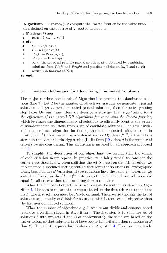
3.1 Divide-and-Conquer for Identifying Dominated Solutions
The major runtime bottleneck of Algorithm1 is pruning the dominated solu-tions (line 9). Let d be the number of objectives. Assume we generate n partialsolutions and get m non-dominated partial solutions, then the naive pruningstep takes O(mnd) time. Here we describe a strategy that significantly boostthe efficiency of the overall DP algorithms for computing the Pareto frontier,which leverages the dimensionality of solutions to efficiently identify the subsetof non-dominated solutions from a set of candidate solutions. The new divide-and-conquer based algorithm for finding the non-dominated solutions runs inO(n(log n)d−1) if we use comparison-based sort or O(n(log n)d−2) if the data isstored in the Lattice Latin Hypercube (LLH) form [19]. Here d is the number ofcriteria we are considering. This algorithm is inspired by an approach proposedin [19].
To simplify the description of our algorithms, we assume that the valuesof each criterion never repeat. In practice, it is fairly trivial to consider thecorner case. Specifically, when splitting the set S based on the dth criterion, weimplemented a modified sorting routine that sorts the solutions in lexicographicorder, based on the dthcriterion. If two solutions have the same dth criterion, wesort them based on the (d − 1)th criterion, etc. Note that if two solutions areequal for all criteria then their ordering does not matter.
When the number of objectives is two, we use the method as shown in Algo-rithm2. The idea is to sort the solutions based on the first criterion (good onesfirst). The first solution must be Pareto optimal. Then, we go through the list ofsolutions sequentially and look for solutions with better second objective thanthe last non-dominated solution.
When the number of objectives d ≥ 3, we use our divide-and-conquer basedrecursive algorithm shown in Algorithm 3. The first step is to split the set ofsolutions S into two sets A and B of approximately the same size based on thelast criterion, so that solutions in A have better last criterion than solutions in B(line 8). The splitting procedure is shown in Algorithm4. Then, we recursively
270 J. M. Gomes-Selman et al.
Algorithm 2. Non Dominated 2D(S): given a set S of 2-dimensional partialsolutions, find the set of non-dominated solutions in S.1 Sort solutions in S by their first element, in descending order if we aim to
maximize the element, in ascending order otherwise;2 P ← {S[1]};3 foreach s ∈ S[2 :] do4 if s is not dominated by the last element of P then5 Append s to P ;6 end
7 end8 return P ;
Algorithm 3. Non Dominated(S): given a set S of d-dimensional partialsolutions (d ≥ 2), find the set of non-dominated solutions in S.1 d ← dimensionality of solutions in S;2 n ← number of solutions in S;3 if n = 1 then4 return S5 else if d = 2 then6 return Non Dominated 2D(S)7 else8 A, B ← Split(S, d);9 A′ ← Non Dominated(A); // solutions in A’ are non-dominated in S.
10 B′ ← Non Dominated(B);11 return A′ ∪ Marry(A′, B′, d − 1);
12 end
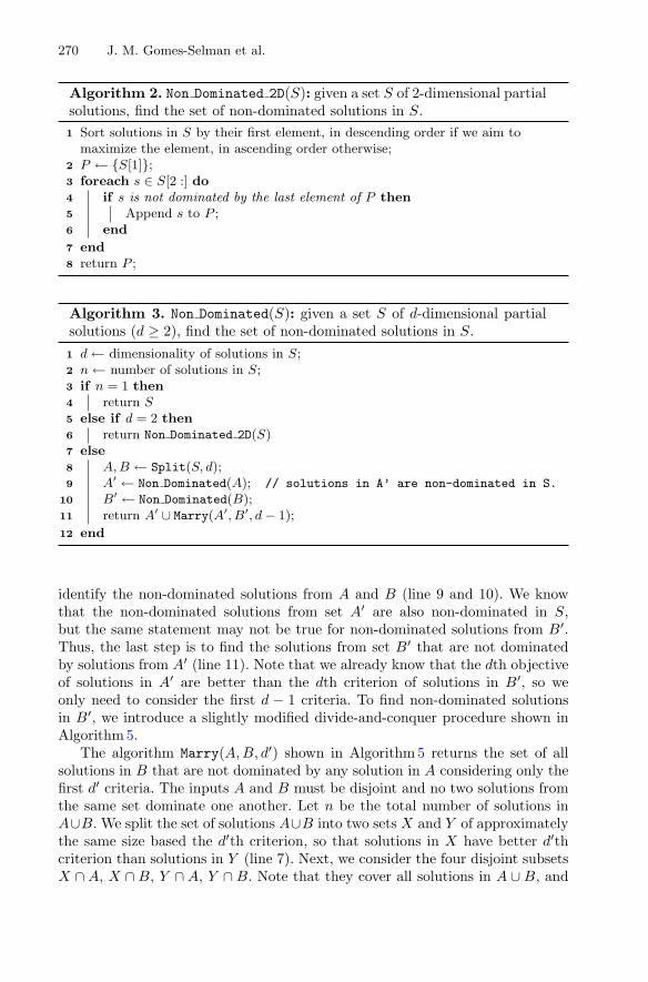
identify the non-dominated solutions from A and B (line 9 and 10). We knowthat the non-dominated solutions from set A′ are also non-dominated in S,but the same statement may not be true for non-dominated solutions from B′.Thus, the last step is to find the solutions from set B′ that are not dominatedby solutions from A′ (line 11). Note that we already know that the dth objectiveof solutions in A′ are better than the dth criterion of solutions in B′, so weonly need to consider the first d − 1 criteria. To find non-dominated solutionsin B′, we introduce a slightly modified divide-and-conquer procedure shown inAlgorithm 5.
The algorithm Marry(A,B, d′) shown in Algorithm5 returns the set of allsolutions in B that are not dominated by any solution in A considering only thefirst d′ criteria. The inputs A and B must be disjoint and no two solutions fromthe same set dominate one another. Let n be the total number of solutions inA∪B. We split the set of solutions A∪B into two sets X and Y of approximatelythe same size based the d′th criterion, so that solutions in X have better d′thcriterion than solutions in Y (line 7). Next, we consider the four disjoint subsetsX ∩ A, X ∩ B, Y ∩ A, Y ∩ B. Note that they cover all solutions in A ∪ B, and
Boosting Efficiency for Computing the Pareto Frontier 271
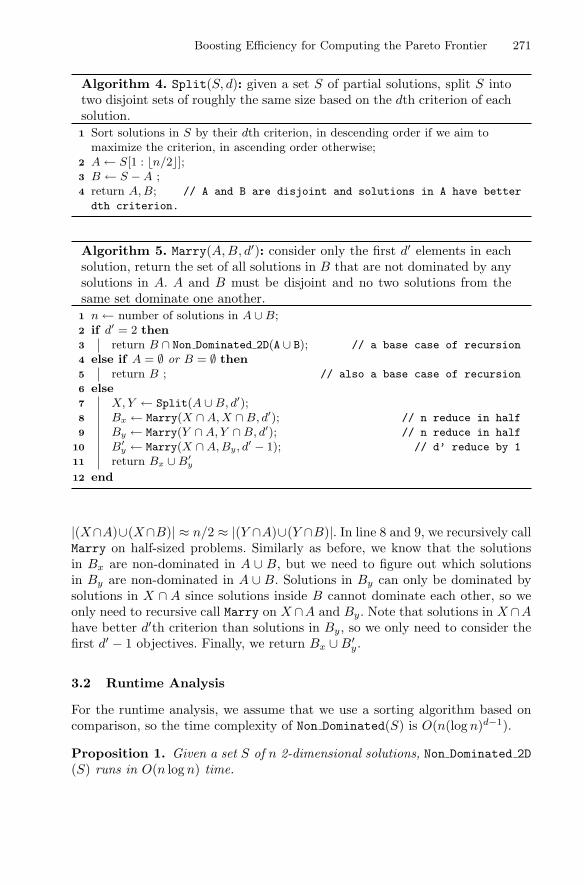
Algorithm 4. Split(S, d): given a set S of partial solutions, split S intotwo disjoint sets of roughly the same size based on the dth criterion of eachsolution.1 Sort solutions in S by their dth criterion, in descending order if we aim to
maximize the criterion, in ascending order otherwise;2 A ← S[1 : �n/2�];3 B ← S − A ;4 return A, B; // A and B are disjoint and solutions in A have better
dth criterion.
Algorithm 5. Marry(A,B, d′): consider only the first d′ elements in eachsolution, return the set of all solutions in B that are not dominated by anysolutions in A. A and B must be disjoint and no two solutions from thesame set dominate one another.1 n ← number of solutions in A ∪ B;2 if d′ = 2 then3 return B ∩ Non Dominated 2D(A ∪ B); // a base case of recursion
4 else if A = ∅ or B = ∅ then5 return B ; // also a base case of recursion
6 else7 X, Y ← Split(A ∪ B, d′);8 Bx ← Marry(X ∩ A, X ∩ B, d′); // n reduce in half
9 By ← Marry(Y ∩ A, Y ∩ B, d′); // n reduce in half
10 B′y ← Marry(X ∩ A, By, d′ − 1); // d’ reduce by 1
11 return Bx ∪ B′y
12 end
|(X∩A)∪(X∩B)| ≈ n/2 ≈ |(Y ∩A)∪(Y ∩B)|. In line 8 and 9, we recursively callMarry on half-sized problems. Similarly as before, we know that the solutionsin Bx are non-dominated in A ∪ B, but we need to figure out which solutionsin By are non-dominated in A ∪ B. Solutions in By can only be dominated bysolutions in X ∩ A since solutions inside B cannot dominate each other, so weonly need to recursive call Marry on X ∩A and By. Note that solutions in X ∩Ahave better d′th criterion than solutions in By, so we only need to consider thefirst d′ − 1 objectives. Finally, we return Bx ∪ B′
y.
3.2 Runtime Analysis
For the runtime analysis, we assume that we use a sorting algorithm based oncomparison, so the time complexity of Non Dominated(S) is O(n(log n)d−1).
Proposition 1. Given a set S of n 2-dimensional solutions, Non Dominated 2D(S) runs in O(n log n) time.
272 J. M. Gomes-Selman et al.
This is because the sorting step takes O(n log n) time and the for-loop takesO(n) time.
Proposition 2. Given a set S containing n solutions, Split(S, d) runs inO(n log n) time.
This is also because the sorting step takes O(n log n) time.
Proposition 3. Given two disjoint sets A and B such that no two solutionsfrom the same set dominate one another and that A ∪ B contains n solutions,Marry(A,B, d′) runs in O(n(log n)d′−1) time.
Proof: We denote the runtime of Marry(A,B, d′) as t(n, d′). For the base cased′ = 2, the proposition obviously holds. For d′
0 ≥ 3, assume the proposition holdsfor d′ < d′
0, which means that t(n, d′0−1) = O(n(log n)d′
0−1−1) = O(n(log n)d′0−2)
for any positive integer n. Now we consider cases where n = 2k for some posi-tive integer k and d′ = d′
0. The major components of Marry are: a Split step(O(n log n) time), two half sized Marry steps (2 t(n/2, d′
0) time), and a Marrystep with dimension reduced by one (t(n, d′
0−1) time). With induction, we knowthat t(n, d′
0 − 1) = O(n(log n)d′0−2). For any positive integer k and n = 2k, we
have
t(2k, d′0) = O(2k log(2k)) + 2 · t((2k)/2, d′
0) + t(2k, d′0 − 1)
= 2 · t(2k−1, d′0) + O(2k · kd′
0−2).
Then, by induction on k, we can prove the following statement
t(2k, d′0) = O(n(log n)d′
0−1).
Since the runtime of Marry increases monotonically with n, the proposition alsoholds when n is not a power of 2. Hence, Marry(A,B, d′) runs in O(n(log n)d′−1)time.
Proposition 4. Given a set S containing n d-dimensional solutions (d ≥ 3),Non Dominated(S) runs in O(n(log n)d−1) time.
Proof: When d ≤ 2, the proposition clearly holds. For d ≥ 3, we denote theruntime as T (n, d). Similarly as in the proof of Proposition 3, we have
T (2k, d) = 2 · T (2k−1, d) + O(2k · kd−2).
Then, by induction on k, we get
T (2k, d) = O(n(log n)d−1).
Since the runtime of Non Dominated(S) increases monotonically with n, theproposition also holds when n is not a power of 2. Hence, Non Dominated(S)runs in O(n(log n)d−1) time.
Boosting Efficiency for Computing the Pareto Frontier 273
3.3 Implementation Notes
Split: The split procedure shown in Algorithm 4 can also be implemented usingan O(n) find median algorithm. However, the numerous steps of copying arraysand creating new arrays in the O(n) find median algorithm are hard to implementand perform poorly in practice. Hence, we chose to use sorting to work “in-place”on the sets of solutions. Each time we drop a dimension we must create a newarray sorted based on that dimension and then in the recursive process we simplykeep track of the location within the array that we are working on. We foundthat in practice sorting and working in place give us much better performance.
Batching: Our new divide-and-conquer algorithm for pruning dominated solu-tions considerably speeds up the DP algorithm and allow us to solve problemson much larger networks, with higher precision, and with more objectives. How-ever, the number of solutions to evaluate grows exponentially with the numberof objectives and memory soon becomes a problem. For example, for the entireAmazon basin, for four criteria, with a precision of ε = 0.01, the algorithm hasto evaluate 144, 823, 974, 336 partial solutions at a single node of the tree, whichis way beyond the memory available. To circumvent this problem, we introduceda batching process: at each tree node, instead of evaluating all possible solutionsat once, we feed them to Non Dominated in smaller batches of size K = 107.Then, we run Non Dominated on the set of all non-dominated solutions fromeach batch. In practice, this batching routine actually also speeds up the DPalgorithm. In the future we plan to consider different batching strategies andalso parallel batching, which can be done in a straightforward way.
4 MIP-Based Pareto Frontier
We also proposed a MIP formulation (see Fig. 3) and a scheme for ε-approximating the Pareto-frontier of a multi-objective optimization problemin [18]. The key idea is to divide the space of objectives into small hyper-rectangles and query whether there exists a feasible solution in each hyper-rectangle. Then, from each feasible hyper-rectangle, we find one solution andform a set S of all the solutions we find. Under the condition that for eachdimension, the upper bound of each hyper-rectangle is (1 + ε) of the lowerbound, the set of non-dominated solutions from S forms an ε-approximatePareto-frontier [9].
In this paper we exploit restart strategy and introduce a new scheme toreduce the number of MIPs to solve. We first optimize for one of the objectives.We divide the space of the remaining objectives into small hyper-rectangles.Specifically, the hyper-rectangles are designed to satisfy the condition that, foreach dimension, the upper bound is (1 + ε) of the lower bound (assuming theobjectives are always positive values). For each cell, we formulate a MIP to findthe solution in that cell that optimizes the target objective if a feasible solutionexists. We form a set S of all the solutions found by MIP. Under the assumption
274 J. M. Gomes-Selman et al.
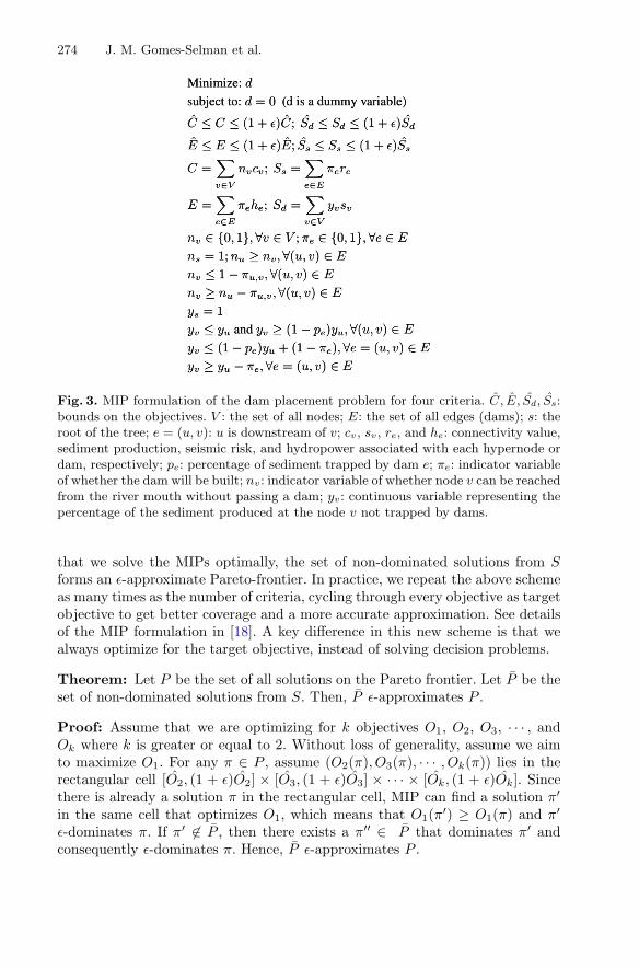
Fig. 3. MIP formulation of the dam placement problem for four criteria. C, E, Sd, Ss:bounds on the objectives. V : the set of all nodes; E: the set of all edges (dams); s: theroot of the tree; e = (u, v): u is downstream of v; cv, sv, re, and he: connectivity value,sediment production, seismic risk, and hydropower associated with each hypernode ordam, respectively; pe: percentage of sediment trapped by dam e; πe: indicator variableof whether the dam will be built; nv: indicator variable of whether node v can be reachedfrom the river mouth without passing a dam; yv: continuous variable representing thepercentage of the sediment produced at the node v not trapped by dams.
that we solve the MIPs optimally, the set of non-dominated solutions from Sforms an ε-approximate Pareto-frontier. In practice, we repeat the above schemeas many times as the number of criteria, cycling through every objective as targetobjective to get better coverage and a more accurate approximation. See detailsof the MIP formulation in [18]. A key difference in this new scheme is that wealways optimize for the target objective, instead of solving decision problems.
Theorem: Let P be the set of all solutions on the Pareto frontier. Let P be theset of non-dominated solutions from S. Then, P ε-approximates P .
Proof: Assume that we are optimizing for k objectives O1, O2, O3, · · · , andOk where k is greater or equal to 2. Without loss of generality, assume we aimto maximize O1. For any π ∈ P , assume (O2(π), O3(π), · · · , Ok(π)) lies in therectangular cell [O2, (1 + ε)O2] × [O3, (1 + ε)O3] × · · · × [Ok, (1 + ε)Ok]. Sincethere is already a solution π in the rectangular cell, MIP can find a solution π′
in the same cell that optimizes O1, which means that O1(π′) ≥ O1(π) and π′
ε-dominates π. If π′ �∈ P , then there exists a π′′ ∈ P that dominates π′ andconsequently ε-dominates π. Hence, P ε-approximates P .
Boosting Efficiency for Computing the Pareto Frontier 275
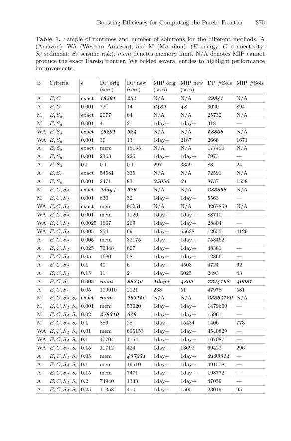
Table 1. Sample of runtimes and number of solutions for the different methods. A(Amazon); WA (Western Amazon); and M (Maranon); (E energy; C connectivity;Sd sediment; Se seismic risk). mem denotes memory limit. N/A denotes MIP cannotproduce the exact Pareto frontier. We bolded several entries to highlight performanceimprovements.
B Criteria ε DP orig(secs)
DP new(secs)
MIP orig(secs)
MIP new(secs)
DP #Sols MIP #Sols
A E, C exact 18291 254 N/A N/A 39841 N/A
A E, C 0.001 72 14 6432 48 3020 894
M E, Sd exact 2077 64 N/A N/A 25732 N/A
M E, Sd 0.001 4 2 1day+ 1day+ 318 —
WA E, Sd exact 46291 924 N/A N/A 58808 N/A
WA E, Sd 0.001 30 13 1day+ 2187 2668 1671
A E, Sd exact mem 15153 N/A N/A 177490 N/A
A E, Sd 0.001 2368 226 1day+ 1day+ 7973 —
A E, Sd 0.1 0.1 0.1 297 3359 83 24
A E, Se exact 54581 335 N/A N/A 72591 N/A
A E, Se 0.001 2471 83 35050 31 8737 1558
M E, C, Sd exact 2day+ 526 N/A N/A 283898 N/A
M E, C, Sd 0.001 630 32 1day+ 1day+ 5563 —
WA E, C, Sd exact mem 90251 N/A N/A 3267859 N/A
WA E, C, Sd 0.001 mem 1120 1day+ 1day+ 88710 —
WA E, C, Sd 0.0025 1667 269 1day+ 1day+ 28804 —
WA E, C, Sd 0.005 254 69 1day+ 65638 12655 4129
A E, C, Sd 0.005 mem 32175 1day+ 1day+ 758462 —
A E, C, Sd 0.025 70348 607 1day+ 1day+ 48381 —
A E, C, Sd 0.05 1680 58 1day+ 1day+ 12866 —
A E, C, Sd 0.1 40 6 1day+ 4503 4724 62
A E, C, Sd 0.15 11 2 1day+ 6025 2493 43
A E, C, Se 0.005 mem 88246 1day+ 4809 2274168 40981
A E, C, Se 0.05 109910 2121 238 51 47978 581
M E, C, Sd, Se exact mem 763150 N/A N/A 23364120 N/A
M E, C, Sd, Se 0.001 mem 53620 1day+ 1day+ 1479660 —
M E, C, Sd, Se 0.02 278310 649 1day+ 1day+ 15961 —
M E, C, Sd, Se 0.1 886 28 1day+ 15484 1406 773
WA E, C, Sd, Se 0.01 mem 695153 1day+ 1day+ 3540829 —
WA E, C, Sd, Se 0.1 47704 1154 1day+ 1day+ 107087 —
WA E, C, Sd, Se 0.15 11712 424 1day+ 13692 69422 296
A E, C, Sd, Se 0.05 mem 437271 1day+ 1day+ 2193314 —
A E, C, Sd, Se 0.1 mem 19510 1day+ 1day+ 491578 —
A E, C, Sd, Se 0.15 mem 7471 1day+ 1day+ 198772 —
A E, C, Sd, Se 0.2 74940 1333 1day+ 1day+ 47059 —
A E, C, Sd, Se 0.25 11358 410 1day+ 1505 23019 95
276 J. M. Gomes-Selman et al.
We observed fat and heavy-tailed behavior in the MIP runtime distribu-tions [7]. To improve performance, we run the MIP solver with a cutoff, using ageometric restart strategy that doubles the cutoff time in every run [7,15]. Ourexperiments show that the restart strategy significantly boosts performance.
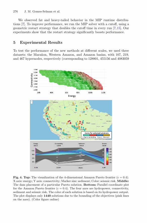
5 Experimental Results
To test the performance of the new methods at different scales, we used threedatasets: the Maranon, Western Amazon, and Amazon basins, with 107, 219,and 467 hypernodes, respectively (corresponding to 128801, 455156 and 4083059
Fig. 4. Top: The visualization of the 4-dimensional Amazon Pareto frontier (ε = 0.4).X axis: energy; Y axis: connectivity; Marker size: sediment; Color: seismic risk. Middle:The dam placement of a particular Pareto solution. Bottom: Parallel coordinate plotfor the Amazon Pareto frontier (ε = 0.4). The four axes are hydropower, connectivity,sediment and seismic risk. The color of each solution is based on its hydropower output.The plot displays only 1440 solutions due to the bounding of the objectives (pink lineson the axes). (Color figure online)
Boosting Efficiency for Computing the Pareto Frontier 277
river segments, respectively). We compare the performance of the new DP andMIP methods with the methods in [18] and see significant improvements in bothspeed and accuracy. See Fig. 1 and Table 1 for a summary of results.
Specifically, in terms of accuracy, the new MIP approach is substantiallybetter than the previous MIP approach. As shown in Fig. 1, in the 2-dimensionalcase, the solutions produced by the new MIP approach are on the exact Paretofrontier, slightly better than the DP approximation for the same ε = 0.1.
The new DP approach has the same high level of accuracy as the previousDP approach and still produces more solutions than the MIP approaches.
In terms of speed, our experiments show that the new DP approach is up tothree orders of magnitude faster than the original DP and scales to significantlylarger instances and more criteria. The batching technique also solves the issueof hitting the memory limit when computing for three or more objectives. Thenew MIP approach is faster and can now solve larger problems.
The DP and MIP methods are complementary since in practice our newMIP scheme provides solutions closer to the exact Pareto frontier (for a given ε)and it provides more flexibility for considering additional constraints for what-ifanalyses, which is important to decision makers.
We are developing a web-based visualization tool for policy makers to explorethe Pareto frontier interactively. For example, Fig. 4 displays: (1) the Paretofrontier for four criteria for the entire Amazon (ε = 0.4); (2) the placement ofthe selected dams for a particular Pareto solution; and (3) a parallel coordinateplots to visualize the solutions, in which each axis represents an objective, andeach line across the different axes represents a solution. We can bound eachobjective (pink lines on the axes) and only show solutions that satisfy the bounds.By bounding each objective appropriately, we notably decrease the number ofsolutions to consider.
6 Conclusions
We introduced new DP and MIP approaches that significantly boost the effi-ciency and accuracy of computing the exact Pareto frontier and its approxima-tion with guarantees on tree-structured networks. Our DP and MIP approachesshow complementary strengths and are now able to scale up to much largerreal-world problems. We are developing interactive tools for what-if analysesand visualizations for policy makers. The overall goal of this project is to assistpolicy makers in making informed decisions when planning hydropower damsin the Amazon Basin. Our methods are general and can be adapted to othermulti-objective optimization problems on tree-structured networks.
Acknowledgments. This work was supported by NSF Expedition awards for Com-putational Sustainability (CCF-1522054 and CNS-0832782), NSF CRI (CNS-1059284)and Cornell University’s Atkinson Center for a Sustainable Future.
278 J. M. Gomes-Selman et al.
References
1. Altwaijry, N., EI Bachir Menai, M.: Data structures in multi-objective evolutionaryalgorithms. J. Comput. Sci. Technol. 27(6), 1197–1210 (2012)
2. Deb, K., Pratap, A., Agarwal, S., Meyarivan, T.: A fast and elitist multiobjectivegenetic algorithm: NSGA-II. IEEE Trans. Evol. Comput. 6(2), 182–197 (2002)
3. Ehrgott, M., Gandibleux, X.: A survey and annotated bibliography of multiobjec-tive combinatorial optimization. OR Spectrum 22(4), 425–460 (2000)
4. Finer, M., Jenkins, C.N.: Proliferation of hydroelectric dams in the Andean Ama-zon and implications for Andes-Amazon connectivity. PLoS One 7(4), e35126(2012)
5. Gavanelli, M.: An algorithm for multi-criteria optimization in CSPs. In: Proceed-ings of the 15th European Conference on Artificial Intelligence, ECAI, pp. 136–140(2002)
6. Gomes, C.P.: Computational sustainability: computational methods for a sustain-able environment, economy, and society. Bridge 39(4), 5–13 (2009)
7. Gomes, C.P., Selman, B., Crato, N., Kautz, H.: Heavy-tailed phenomena in sat-isfiability and constraint satisfaction problems. J. Auto. Reason. 24(1), 67–100(2000)
8. Neumann, F.: Expected runtimes of a simple evolutionary algorithm for the multi-objective minimum spanning tree problem. Eur. J. Oper. Res. 181(3), 1620–1629(2007)
9. Papadimitriou, C.H., Yannakakis, M.: On the approximability of trade-offs andoptimal access of web sources. In: Proceedings of the 41st Annual Symposium onFoundations of Computer Science, FOCS 2000 (2000)
10. Qian, C., Tang, K., Zhou, Z.-H.: Selection hyper-heuristics can provably be helpfulin evolutionary multi-objective optimization. In: Handl, J., Hart, E., Lewis, P.R.,Lopez-Ibanez, M., Ochoa, G., Paechter, B. (eds.) PPSN 2016. LNCS, vol. 9921, pp.835–846. Springer, Cham (2016). https://doi.org/10.1007/978-3-319-45823-6 78
11. Qian, C., Yu, Y., Zhou, Z.-H.: Pareto ensemble pruning. In: Proceedings of theTwenty-Ninth AAAI Conference on Artificial Intelligence, AAAI 2015, pp. 2935–2941 (2015)
12. Schaus, P., Hartert, R.: Multi-objective large neighborhood search. In: Schulte, C.(ed.) CP 2013. LNCS, vol. 8124, pp. 611–627. Springer, Heidelberg (2013). https://doi.org/10.1007/978-3-642-40627-0 46
13. Sheng, W., Liu, Y., Meng, X., Zhang, T.: An improved strength pareto evolution-ary algorithm 2 with application to the optimization of distributed generations.Comput. Math. Appl. 64(5), 944–955 (2012)
14. Terra-Neves, M., Lynce, I., Manquinho, V.: Introducing pareto minimal correctionsubsets. In: Gaspers, S., Walsh, T. (eds.) SAT 2017. LNCS, vol. 10491, pp. 195–211.Springer, Cham (2017). https://doi.org/10.1007/978-3-319-66263-3 13
15. Walsh, T.: Search in a small world. In: Proceedings of the 16th International JointConference on Artificial Intelligence, IJCAI 1999, San Francisco, CA, USA, vol. 2,pp. 1172–1177. Morgan Kaufmann Publishers Inc. (1999)
16. Wiecek, M.M., Ehrgott, M., Fadel, G., Figueira, J.R.: Multiple criteria decisionmaking for engineering (2008)
17. Winemiller, K.O., McIntyre, P.B., Castello, L., Fluet-Chouinard, E., Giarrizzo,T., Nam, S., Baird, I.G., Darwall, W., Lujan, N.K., Harrison, I., et al.: Balanc-ing hydropower and biodiversity in the Amazon, Congo, and Mekong. Science351(6269), 128–129 (2016)

Boosting Efficiency for Computing the Pareto Frontier 279
18. Wu, X., Gomes-Selman, J.M., Shi, Q., Xue, Y., Garcia-Villacorta, R., Sethi, S.,Steinschneider, S., Flecker, A., Gomes, C.P.: Efficiently approximating the paretofrontier: hydropower dam placement in the Amazon basin. In: AAAI (2018)
19. Yukish, M.: Algorithms to identify Pareto points in multi-dimensional data sets.Ph.D. thesis (2004)
20. Yukish, M., Simpson, T.W.: Analysis of an algorithm for identifying pareto pointsin multi-dimensional data sets. In: 10th AIAA/ISSMO Multidisciplinary Analysisand Optimization Conference, p. 4324 (2004)
21. Zarfl, C., Lumsdon, A.E., Berlekamp, J., Tydecks, L., Tockner, K.: A global boomin hydropower dam construction. Aquat. Sci. 77(1), 161–170 (2015)
22. Ziv, G., Baran, E., Nam, S., Rodrıguez-Iturbe, I., Levin, S.A.: Trading-off fishbiodiversity, food security, and hydropower in the Mekong River Basin. Proc. Nat.Acad. Sci. 109(15), 5609–5614 (2012)