Bootstrapping in R – A Tutorial

Eric B. Putman

Department of Ecosystem Science and Management

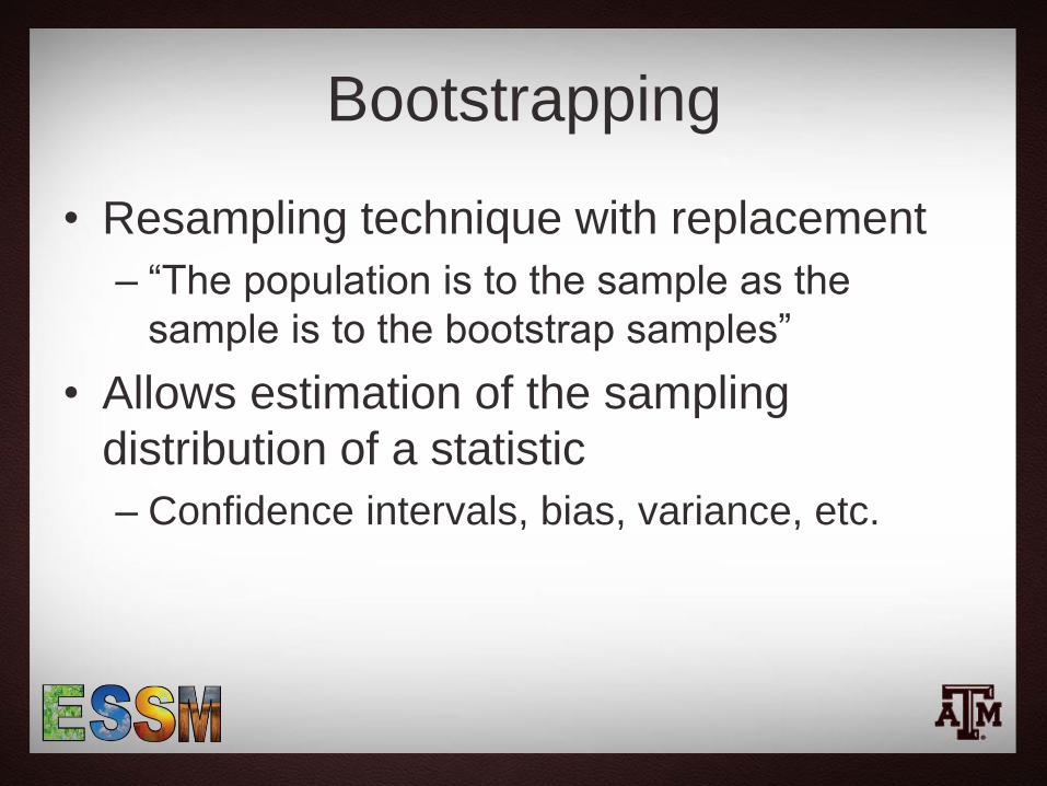
Bootstrapping

• Resampling technique with replacement

– “The population is to the sample as the

sample is to the bootstrap samples”

• Allows estimation of the sampling

distribution of a statistic

– Confidence intervals, bias, variance, etc.

Procedure

• Resample a dataset a given number of

times

• Calculate a statistic from each sample

• Accumulate the results and calculate

sample distribution of the statistic

Objective

• Calculate a series of linear regressions to determine which variable or combination of variables best explains the volume of black cherry trees

– Comparisons made using coefficient of determination (R-squared)

• Bootstrap the linear regressions (for each bootstrap sample) to determine 95% confidence intervals of their respective R-squared values

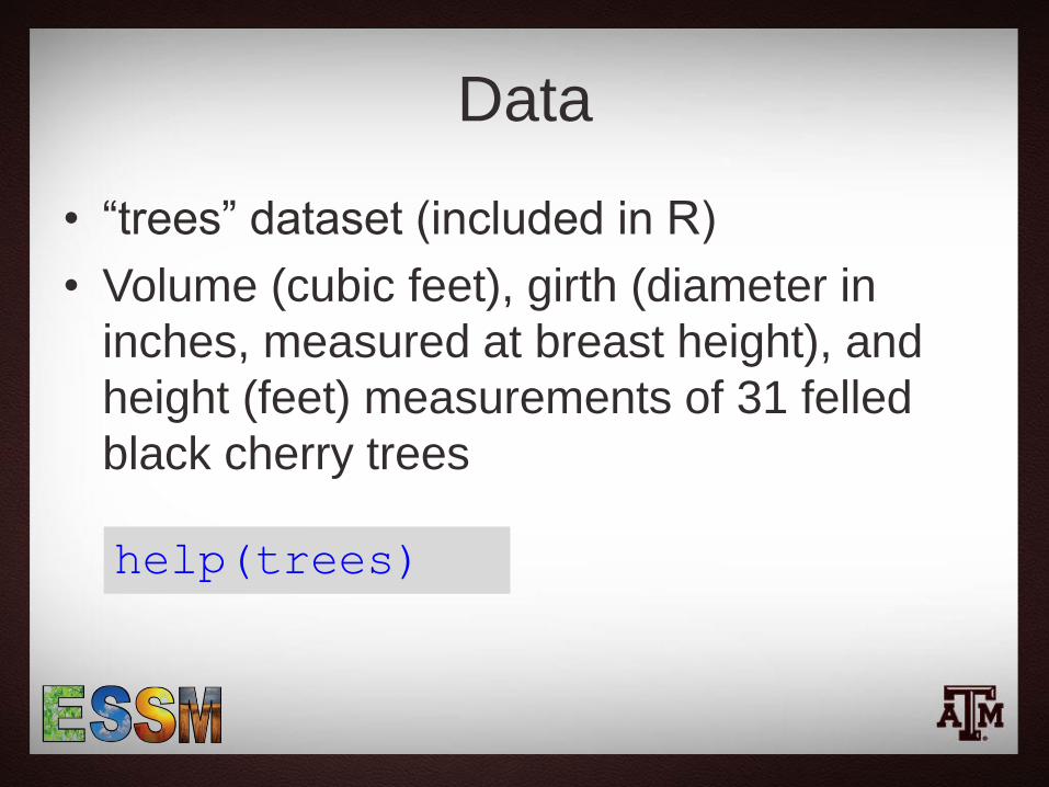
Data

• “trees” dataset (included in R)

• Volume (cubic feet), girth (diameter in

inches, measured at breast height), and

height (feet) measurements of 31 felled

black cherry trees

help(trees)

Code Walkthrough

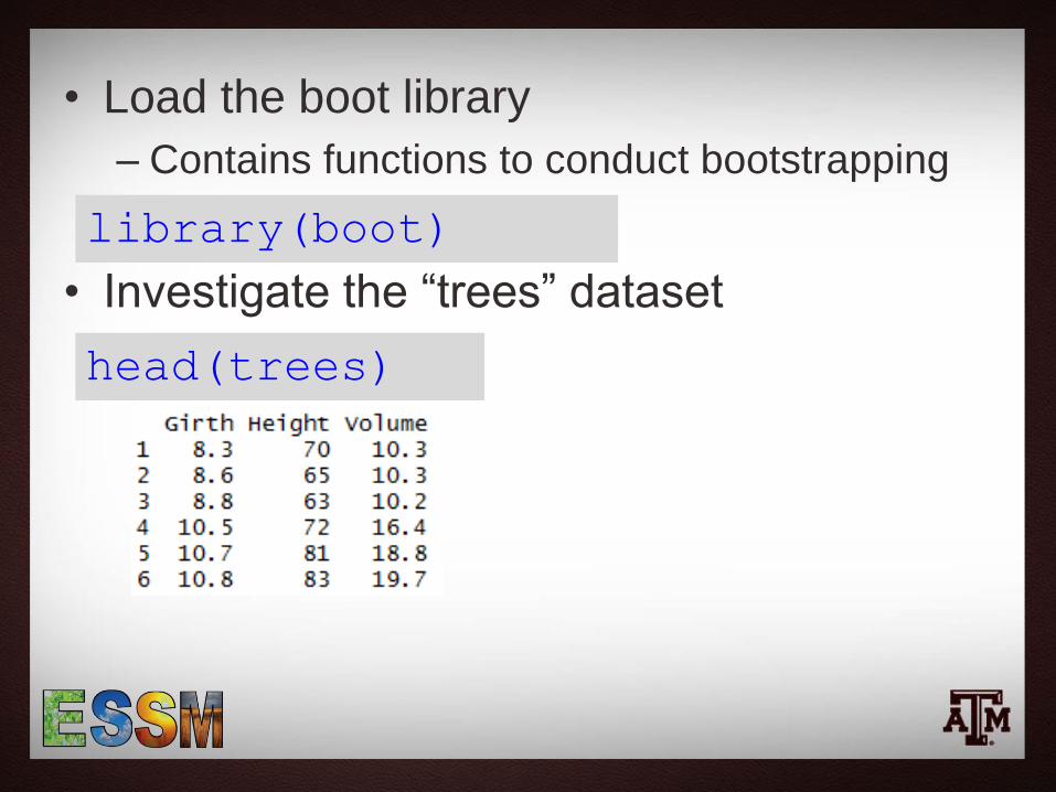
• Load the boot library

– Contains functions to conduct bootstrapping

• Investigate the “trees” dataset

head(trees)

library(boot)

• Explore relationships between volume,

girth, and height plot(trees$Volume~trees$Height, main = 'Black Cherry Tree Volume

Relationship', xlab = 'Height', ylab = 'Volume', pch = 16, col =

'blue')

plot(trees$Volume~trees$Girth, main = 'Black Cherry Tree Volume

Relationship', xlab = 'Girth', ylab = 'Volume', pch = 16, col =

'blue')

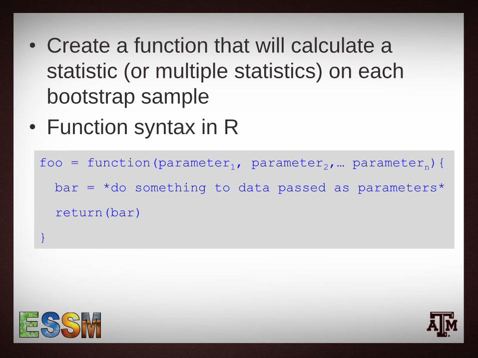
• Create a function that will calculate a

statistic (or multiple statistics) on each

bootstrap sample

• Function syntax in R

foo = function(parameter1, parameter2,… parametern){

bar = *do something to data passed as parameters*

return(bar)

}

• Statistic-calculation function for the boot package takes

two specific parameters (simple example) and will be

applied to each bootstrap sample

sample_mean = function(data, indices){

sample = data[indices, ]

bar = mean(sample)

return(bar)

}

Creates the bootstrap sample (i.e.,

subset the provided data by the

“indices” parameter). “indices” is

automatically provided by the “boot”

function; this is the sampling with

replacement portion of bootstrapping

Calculate the mean of

the bootstrap sample

sample_mean = function(data, indices){

return(mean(data[indices]))

}

Or, more concisely:

• Create a function to calculate linear regressions of several variable

combinations and return their respective R-squared values – Height only,

– Girth only

– Girth / height ratio

– Girth and height

– Girth, height, and girth / height ratio

• Note that we are calculating (and returning) multiple statistics simultaneously – These statistics will be calculated for each bootstrap sample

volume_estimate = function(data, indices){

d = data[indices, ]

H_relationship = lm(d$Volume~d$Height, data = d)

H_r_sq = summary(H_relationship)$r.square

G_relationship = lm(d$Volume~d$Girth, data = d)

G_r_sq = summary(G_relationship)$r.square

G_H_ratio = d$Girth / d$Height

G_H_relationship = lm(d$Volume~G_H_ratio, data = d)

G_H_r_sq = summary(G_H_relationship)$r.square

combined_relationship = lm(d$Volume~d$Height + d$Girth, data = d)

combined_r_sq = summary(combined_relationship)$r.square

combined_2_relationship = lm(d$Volume~d$Height +d$Girth + G_H_ratio, data = d)

combined_2_r_sq = summary(combined_2_relationship)$r.square

relationships = c(H_r_sq, G_r_sq, G_H_r_sq, combined_r_sq, combined_2_r_sq)

return(relationships)

}

Statistics are added to a vector, which is then

returned to the “boot” function

• Conduct the bootstrapping

– Use “boot” function

results = boot(data = trees, statistic = volume_estimate, R = 5000)

Dataset from which statistics

will be calculated

Function we created to

calculate statistics on each

bootstrap sample

Number of bootstrap samples (i.e.,

iterations)

• View some calculated statistics of boot

object

print(results)

t* corresponds to index of

“relationships” vector (e.g., t1*

refers to height only R-squared

value

• Plot the boot objects

– Provides histogram and Q-Q plot

plot(results, index = 1)

The index parameter corresponds to the indices of the vector

(“relationships”) returned by the “volume_estimation” function (e.g., index 1 is

the first item in the vector, which is the height only R-squared value)

relationships = c(H_r_sq, G_r_sq, G_H_r_sq, combined_r_sq, combined_2_r_sq)

Height only R-squared

distribution:

• Calculate 95% confidence intervals for

each of the bootstrapped R-squared values

– Using “Bias Corrected and Accelerated” (BCa)

method

confidence_interval_H = boot.ci(results, index = 1, conf = 0.95, type = 'bca')

print(confidence_interval_H)

ci_H = confidence_interval_H$bca[ , c(4, 5)]

print(ci_H)

Specify index corresponding to position in

vector for each statistic

Store confidence intervals in a

variable in order to plot later

• View histograms (frequency and density)

• Add kernel density line (blue)

• Add 95% confidence intervals (red) hist(results$t[,1], main = 'Coefficient of Determination: Height', xlab = 'R-

Squared', col = 'grey')

hist(results$t[,1], main = 'Coefficient of Determination: Height', xlab = 'R-

Squared', col = 'grey', prob = T)

lines(density(results$t[,1]), col = 'blue')

abline(v = ci_H, col = 'red')

Note syntax to call desired sample distribution

• Can also call the entire sample distribution

to further manipulate, save, etc.

results$t[ , 1]

Access the sample statistics of each bootstrap

sample

Subset to particular

statistic; first column of

the boot object “t”

corresponds to the first

item in the vector

returned by the

“volume_esitmate”

function R-squared values of height only linear regression:

Results • Linear regression with explanatory variables of girth,

height, and girth / height ratio provided best coefficients

of determination to model the volume of black cherry

trees

• 5,000 sample bootstrap allowed estimation of R-squared

sampling distribution

– Could have also bootstrapped values of coefficients, additional models, etc.

Original Value Bias Std. Error 95% Confidence Interval

Height Only 0.3579026 0.002405194 0.1202542 0.1414861 - 0.6122950

Girth Only 0.9353199 0.000549577 0.01751679 0.8770796 - 0.9582597

Girth / Height 0.7309204 0.002515606 0.08064029 0.4782823 - 0.8421099

Girth and Height 0.94795 0.003285168 0.01210484 0.9052392 - 0.9647783

Girth, Height, and

Girth / Height0.9732894 0.000544716 0.01042662 0.9418756 - 0.9868528

Estimating Black Cherry Tree Volume - Linear Regression Coefficients of Determination

http://www.statmethods.net/advstats/bootstrapping.html

http://www.mayin.org/ajayshah/KB/R/documents/boot.html

http://www.r-bloggers.com/bootstrap-example/

http://cran.r-project.org/web/packages/boot/boot.pdf

References