borehole geophysical methods for analyzing specific

Borehole Geophysical Methods for Analyzing Specific Capacity of Multiaquifer Wells

GEOLOGICAL SURVEY WATER-SUPPLY PAPER 1536-A

Prepared in cooperation with the Pennsylvania Topographic and Geologic Survey, Department of Internal Affairs

Property of

U.S. GEOLOGICAL SIWVEYWATER RESOURCE: DIVISION

CROUND WATER IRANCHTrenton, New Jersey

Borehole Geophysical Methods for Analyzing Specific Capacity of Multiaquifer WellsBy GORDON D, BENNETT and EUGENE P. PATTEN, JR.

GROUND-WATER HYDRAULICS

GEOLOGICAL SURVEY WATER-SUPPLY PAPER 1536-A

Prepared in cooperation with the Pennsylvania Topographic and Geologic Survey, Department of Internal Affairs

Property of

U.S. GEOLOGICAL SURVEYWATER RESOURCES DIVISION

GROUND WATER IRANCH

Trenton, New Jersey

UNITED STATES GOVERNMENT PRINTING OFFICE, WASHINGTON : 1960

UNITED STATES DEPARTMENT OF THE INTERIOR

FRED A. SEATON, Secretary

GEOLOGICAL SURVEY

Thomas B. Nolan, Director

For sale by the Superintendent of Documents, U.S. Government Printing Office Washington 25, D.G.

CONTENTS

PageAbstract.-..----._________________________________________________ 1Introduction._____________________________________________________ 1Review of earlier work.____-__.____________________________________ 3

Conventional logging and interpretation.____-____-_-________-_--_ 3Flow measurement_________-_.________________-_-__-___--_-_ 3Quantitative hydrology______________________________________ 3

Theoretical considerations and definitions___________________________ 7Specific capacity for varying discharge and drawdown._____________ 7Modifications in the definition of specific capacity _________________ 9Specific capacity of a multiaquifer well__---------_-__----_------- 11Contribution of individual aquifers to specific capacity_---_.__---_- 11Hydraulics of a multiaquifer well.__________________-_--_-----___ 13Method of presentation of experimental data____________________ 17

Description of field tests and calculations____________-_-_-__._-------- 18Equipment-_-_-___________________.____--_______-_----------- 18Experimental procedure_______________-_________-_-___._------- 20

Presentation and evaluation of results_______-_____________------__- 23Conclusions_ _-__________-_____-__-_____-_-_-_-_--_----_---_----_ 24Literature cited___________________________________________________ 25

ILLUSTRATIONS

Page FIGTTHE 1. Conventional specific-capacity graph where water level is

plotted as drawdown, sw_i__________-___-_-_-_-_-_----- 62. Specific capacity at constant discharge and at constant draw

down _-___________-______-______-_____-_-_-_---_----- 73. Specific-capacity graph where water level is plotted as head

above datum_______________________________________ 104. Composite specific-capacity graph for test well for pumping

times of 1 hour_-________----_--_-___------------------ 145. Schematic diagram of conditions in test well not being pumped- 166. Physical and electric logs of test well_________.-_-__--_-__ 197. Schematic diagram of equipment at test well, showing brine-

tracing procedure.. ___________-_-__-_----_----------- 208. Fluctuations of water level due to pumping of test well __ 21

TABLES

TABLE 1. Summary of experimental data_________________-__----_- 222. Data obtained from specific-capacity graph of figure 4____-__- 24

m

GROUND-WATER HYDRAULICS

BOREHOLE GEOPHYSICAL METHODS FOR ANALYZING SPECIFIC CAPACITY OF MULTIAQUIFER WELLS

By GORDON D. BENNITT and EUGENE P. PATTEN, JB.

ABSTRACT

Conventional well-logging techniques, combined with measurements of flow velocity in the borehole, can provide information on the discharge-drawdown characteristics of the several aquifers penetrated by a well. The information is most conveniently presented in a graph showing aquifer discharges as functions of the water level in the well at a particular time.

To determine the discharge-drawdown characteristics, a well is pumped at a steady rate for a certain length of time. While the well is being pumped, meai- urements are made of drawdown and of the discharge rates of the individual aquifers within the well. Discharge rates and drawdowns are usually recorded as functions of time, and their values for any given time during the test are obtained by interpolation. The procedure is repeated for several different rates of total well discharge. The well may be allowed to recover after each step, or discharge may be changed from one rate to another, and changes in discharge and drawdown may be measured by extrapolation. The flow measurements within the well may be made by use of a subsurface flowmeter or by one of several techniques involving the injection of electrolytic or radioactive tracers.

The method was tested on a well in Mercer County, Pa., and provided much useful information on aquifer yields, "thieving," and hydrostatic heads of the individual zones.

INTRODUCTION

The U.S. Geological Survey, in cooperation with the Pennsylvania Topographic and Geologic Survey, has conducted an extensive well- logging program in Pennsylvania since 1956. Water wells throughout the State have been investigated with devices that measure self- potential, point resistance, normal resistivity, temperature, fluid resistivity, borehole diameter, gamma radiation, and flow velocity.

The general objectives of this program were twofold: (a) the accumulation of geologic and hydrologic information in various parts of the State and (b) the development of new methods of interpreting the data of borehole geophysics in ground-water studies. Pursuit of this second objective was undertaken in order to find new or improved approaches to certain hydrologic problems. One such problem is that of the multiaquifer well the well yielding water from two or more

1

2 GROUND-WATER HYDRAULICS

aquifers. Jones and Skibitzke (1956, p. 292) suggest a method of log interpretation designed especially to deal with this problem. The theory underlying their method is described in detail in the following pages, and the results of some field tests are given.

The standard well-logging methods have all been in use for some time in hydrologic work, but the general practice has been to adopt (with little or no modification) the interpretive principles of the oil industry. The quality of the results thus obtained has not been consistent. When the assumptions implicit in the oil-well techniques have been met in the ground-water problem at hand, results have been excellent; when these assumptions have not been met, results have been correspondingly poor. In any event the parallels between oil-reservoir problems and hydrologic problems do not extend in definitely. The future of well logging as a hydrologic tool depends, therefore, upon the development of new interpretive techniques suited especially to the problems of hydrology.

The methods of well logging and interpretation discussed in this paper have as their objective the determination of the discharge- drawdown relations of the individual aquifers supplying a multiaquifer well. The well is pumped at a given discharge rate for a certain length of time. While the well is being pumped, measurements are made of the drawdown in the well and of the discharge rates of the individual aquifers tapped by the well. Discharge rates and drawdowns are usually recorded as functions of time, and their values for any given time during the test are obtained by interpolation. The procedure is repeated for several different rates of well discharge. The well may be allowed to recover after each step, or discharge may be changed directly from one rate to another, and changes in dis charge and drawdown may be measured by extrapolation. The flow measurements may be made by use of a subsurface flowmeter or by one of several techniques involving the injection of electrolytic or radioactive tracers. A normal-resistivity logging device was used to locate the possible aquifers, and a well caliper was used to obtain borehole area at points of velocity measurement.

The authors were fortunate in having at their disposal several methods of flow measurement, and the tests described in this paper were made by the methods that seemed best suited to the particular situation at hand. A detailed discussion of the relative merits of the various techniques of measurement is beyond the scope of the present paper.

A somewhat lengthy discussion of theory is necessary to clarify both the merits and the limitations of the methods under study. This discussion pertains in part to borehole geophysical methods and in

SPECIFIC CAPACITY OF MULTIAQUIFER WELLS 3

part to general ground-water hydrology. It involves a review of some earlier work and the introduction of certain new definitions.

The investigation was made under the immediate supervision of D. W. Greenman, formerly district geologist, U.S. Geological Survey, Harrisburg, Pa.

REVIEW OF EARLIER WORK

CONVENTIONAL LOGGING AND INTERPRETATION

Of the earlier papers on the application of borehole geophysics to ground water, only those of Bays and Folk (1944) and Jones and Skibitzke (1956) are of direct concern to the present problem. Bays and Folk (1944) suggested the use of brine as a flow tracer. Jones and Skibitzke (1956), in their discussion of flowmeter interpretation, suggested the methods forming the basis of the present study.

Various conventional logging techniques and methods of inter pretation can be used to investigate geologic conditions in a well and to locate possible aquifers. The original publications describing these techniques are not reviewed here, for they are adequately sum marized by Jones and Skibitzke (1956).

FLOW MEASUREMENT

Meinzer (1928) reported the use of a conventional Price current meter to detect leaking or "thieving" zones in wells in Hawaii. Fied- ler (1928) described the use of the Au current meter, a mechanical device designed specifically for well-flow measurement. Skibitzke outlined the theory for a thermal well-velocity meter in a Government patent (1955) ; he has since then developed an instrument of this type.

Bird and Dempsey (1955), in a paper intended primarily for appli cation in the oil industry, described a use of radioactive tracers that might be adapted for the measurement of flow in water wells. A method of discharge measurement described by Barbagelata (1928), may be modified for application in a well by using a fluid-conductivity logging device and a suitable brine injection apparatus.

QUANTITATIVE HYDROLOGY

The equation of ground-water flow as given by Jacob (1950, p. 333) for a single, infinite, homogeneous, and isotropic aquifer of uniform thickness, in which there is no vertical flow, is as follows:

where h represents the head, or elevation above datum of the piezometric surface ; $ is the storage coefficient, a dimensionless term defined


as the volume of water released from or taken into storage per unit surface area of the aquifer per unit change in the component of head normal to that surface; and T is the transmissibility of the aquifer, or its permeability multiplied by its thickness, having the dimensions of length squared per unit of time.

The solution for equation 1, for radial flow to a well discharging at a constant rate Q and involving no recharge to the aquifer, is that given by Theis (1935), which may be written as

^rlS

where s is the drawdown at a distance r from the discharging well, at time t after the beginning of pumping. The drawdown is evaluated as the sum of an infinite number of elemental drawdown increments, each the result of an instantaneous discharge at some earlier time, t'; this discharge acts over a time interval dt' .

The integral in equation 2 is evaluated by means of an infinite series

__+ - (3) ^ ^ {J

After a short time of pumping has elapsed, the series terms after the first two become negligibly small, and equation 2 may then be written as

2.25Tt ,..

The drawdown at the discharging well after a sufficient lapse of time is given by equation 4, where rw , the radius of the well, is used in place of r:

2.30a 2.25* , K .

In addition to the drawdown predicted by equation 5, there will generally be a loss of head at the discharging well, representing the energy expended as the water enters the well itself and flows upward through the borehole. Rorabaugh (1953) has indicated that in a typi-

SPECIFIC CAPACITY OF MULTIAQUIFER WELLS "5

cal 12-inch well these losses will be approximately proportional to the first power of the discharge for discharges of less than 0.75 cfs (cubic feet per second) or 337 gpm (gallons per minute). Then the draw down at the discharging well will be

where C' is the constant factor relating entrance head losses to dis charge in this range of discharge values.

For higher values of discharge Rorabaugh indicates well entrance losses proportional to some higher power, n, of the discharge, where the drawdown at the discharging well becomes

2.25Tt

In equation 7, C is the well-loss constant in effect for the higher discharge range.

In the discharge range covered by equation 6, drawdown is readily observed to be a linear function of discharge, if pumping for equal intervals of time is understood. If a well is pumped at several rates of discharge, starting at zero drawdown and continuing for the same length of time at each pumping rate, the resultant drawdowns should plot as a straight line against the corresponding discharge rates. Such a plot is shown in figure 1 , with drawdown on the abscissa and discharge on the ordinate.

The slope of this graph, - } is known as the "specific capacity"ASm

of the well. If the graph were extended into higher rates of dis charge, it would assume some curvature, as can be demonstrated by solving equation 7 for the ratio Q/sw . An examination of equations 6 and 7 will show also that specific capacity is a function of time. After a sufficient time has passed, however, the changes in specific capacity per unit change in time become quite small, so that con siderable differences in the time of pumping at the various discharge rates can often be tolerated.

Jacob and Lohman (1952) have demonstrated that, after a reason able time of pumping, discharge-drawdown points determined by pump ing a well at a variable rate so as to maintain a constant drawdown value approach very closely those determined by discharging the well at a constant rate.

546681 O 6C


The solution of equation 1 given by Jacob and Lohman for this case is

Q=2rrsw.(9(a), (8)

in which sw is the constant drawdown, Q is a function varying with time,

and Y0(x) and Jg (x) are Bessel functions of zero order of the first and second kinds, respectively. The integral is approximated by numeri cal methods, -and a table of values of G(a) for various values of a appears in the reference.

Jacob and Lohman point out that, at large relative values of t, the value of 0(ot) approaches that of the function

0/0012/2.3 log 2.257V

and that the specific-capacity ratio calculated from equation 8 will therefore approach the specific capacity calculated from equation 5.

0 DRAWDOWN (sw ), IN FEET BELOW STATIC WATER LEVEL

FIGUBE 1. Conventional specific-capacity graph where water level is plotted as drawdown, «

SPECIFIC CAPACITY OF MULTIAQUIFEE WELLS

Constant discharge^

Constant drawdown'

0 TIME -

FIOUBE 2. Specific capacity at constant discharge and at constant drawdown.

Jacob and Lohman present a graph (see fig. 2) in which specific capacity is shown as a function of tune for both constant-discharge and constant-drawdown methods.

THEORETICAL CONSIDERATIONS AND DEFINITIONS

SPECIFIC CAPACITY FOB VARYING DISCHARGE AND DRAWDOWN

Equations 5 and 8 form the basis of most of the discharging-wel techniques presently employed in quantitative hydrology, and the only published analytical expressions for the specific-capacity ratio are taken from these equations. They are particular solutions of equation 1, corresponding to two possible ways of discharging an aquifer. Their applicability to multiaquifer problems is not limited by the fact that they were derived in terms of a single aquifer, but rather by their basic assumptions, which demand either a constant rate of discharge or a constant drawdown. Equation 5 could be applied in turn to each individual aquifer in a multiaquifer well, if some means could be found to hold the discharge of each aquifer con stant. Equation 8 likewise could be applied to each aquifer in turn if the drawdown of the well were held constant, head losses within the borehole between aquifers were negligible, and some means were used to measure the variations in discharge of each aquifer with time.

In general, however, neither the drawdown of the well nor the discharges of the various individual aquifers remain constant during the pumping of a multiaquifer well. It will be instructive, therefore,


to supplement the theory reviewed above with a discussion of discharge under more general conditions, in which the rate of discharge and the drawdown are at liberty to vary.

The solution of equation 1 corresponding to these conditions is

This is a more general form of equation 2, in which Q, as a function of time, appears under the integral rather than outside it. As in equation 2, the total drawdown sw at time t is evaluated as the sum of an infinite number of elemental drawdown increments, each of which is the result of the action of the pump during some earlier time interval, of length dt' '. The solution is taken by analogy from that given for the equivalent heat-conduction problem by Carslaw and Jaeger (1959, p. 261).

It is not necessary for the purposes of this paper to find solution of equation 9 corresponding to various possible forms of the function Q,(t'}. The point of direct concern is whether a point (sw , Qw ) reached on the specific-capacity graph by discharge under these general conditions will appreciably differ from that reached by discharge at a constant rate or a constant drawdown for an equal time interval. If the difference is negligible, specific-capacity points taken at variable discharges may be plotted on the same grajih as those taken at constant discharge, and the plot should remain approximately linear. The question in explicit terms is whether or not sw as evaluated by equation 9 will be approximately equal to sw as evaluated by equation 2 if the constant Q of equation 2 is equal to Q(t) in equation 9. [Q(t) is here intenv, ] to mean Q(t f ) evaluated at t'=t.]

An examination of the two equations will show that the answer to this question is dependent upon the nature of the function Q(t'). If this function has a time derivative which approaches zero as t' increases, the discharge eventually appears nearly constant over long time intervals, and the significant variations in discharge are confined to the early periods of pumping. Unless these early varia tions in discharge are excessively large, the nature of the function

t_ t f&xp ( ±T(i"Lt'\ ) *8 8Ucn tnat at larSe values of t the effect of the early

periods of pumping, for which t is very much greater than t', is quite small. The drawdown is largely the result of the operation of the pump at an essentially constant rate during later intervals of pumping and, as such, will not differ greatly from the drawdown predicted by equation 2 for the same value of t. Consequently, at sufficient values of t the ratio QJsw calculated for a constant discharge, Qi, should be


approximately equal to the ratio Q(t)fsw calculated for a time-varying discharge in which

as

It will become clear during the discussion of the discharge of an individual aquifer to a multiaquifer well that in such discharge the condition of a continuously decreasing time derivative of Q(t') is nearly always satisfied, and the initial variations themselves are moderate. Thus it seems reasonable to expect that rpecific-capacity points taken for these aquifers under variable-discharge conditions will plot in approximately the same place as those taken at constant discharge, if the time of pumping is sufficient. (Equation 6 should then approximate the relation between well drawdown and aquifer discharge.) If doubt exists as to the length of a sufficient time of pumping, Q(t') may be recorded in the field as a function of t' . Oc casionally it may be desirable to establish the trend of the function Q(t') in the field and extrapolate this trend to obtain the discharge corresponding to a longer time of pumping.

MODIFICATIONS IX THE DEFINITION OF SPECIFIC CAPACITY

It is sometimes preferable to speak of well "head level" above some datum rather than well drawdown, because the former term is better suited to problems in which the water level in the well may either rise above the nonpumping head of a particular aquifer or be drawn down below it. For such a problem the graph of figure 1 would be replotted as shown in figure 3. Values of Q lying above the horizon tal axis represent discharge; those below represent recharge or input to the well. The specific-capacity graph crosses the horizontal axis at the point

Q=0

h=h0,

where h0 is the static (nonpumping) level of water in the well. In figure 3 the head increases to the right, indicating a higher water level. In figure 1 the converse is ^rue, inasmuch as drawdown increases to the right. Whereas specific capacity was defined as the slope of the graph of figure 1, it will be the negative of the slope of the graph of figure 3. The same statements and equations that apply to discharge can be made regarding well input; the only differences that need be introduced are the use of

fig flip

in place of sw, and the use of the negative sign to distinguish recharge.


HEAD (/,), IN FEET ABOVE ARBITRARY DATUM

FIGURE 3. Specific-capacity graph where water level is plotted as head above datum.

In a well penetrating a single aquifer, the discharge of the aquifer is zero when the water level in the well is at its static level (zero drawdown). Here it is not necessary to use the notation A<2/Asw for specific capacity; we may simply use Qlsw . In work with multiaquifer wells, however, it is necessary to use the graph-slope defini tion, A#/Asw . Equations 5-9 do not demand that the initial values of Qw and sw be zero, because as long as the original amounts and trends of these quantities can be extrapolated and their effect removed from the data under consideration, the equations still apply.

If in equation 6 the symbol B is substituted for the quantity2.3 , 2.25T* i, .. ,-r-ffi log 2cr> the equation becomes

47T2 Tw 'O

sw=BQ+C'Q. (10)

The slope of a graph of Q versus sw then becomes A<2/Asw=l/ (B-\-Cr ), and the slope of a graph of Q versus head, hw, becomes

'B+C'' (ID


It was indicated in the preceding section that, within certain restrictions, points on the specific-capacity graph are largely inde pendent of the manner in which they are approached. Thus equation 11 may be considered a generally valid expression for specific capacity when discharge varies.

The quantitative theory developed heretofore has all been based on the assumption of an infinite, homogeneous, and isotropic aquifer. This is not to say, however, that the ratio AQ/As«, cannot be defined and have meaning unless these conditions are met. A solution zone in limestone, for example, or a fracture zone in crystalline rock may show a constant ratio of discharge to drawdown; the value of this ratio in itself constitutes useful information, even though an analytical expression such as that proceeding from equation 6 cannot be written for it.

SPECIFIC CAPACITY OF A MULTIAQUIFER WELL

The specific capacity of a multiaquifer well is defined in the same way as that of a single-aquifer well: it is the ratio of the change in well discharge to the accompanying change in drawdown of water level. There are two possible ways of writing an analytical expres sion for specific capacity. One is based upon equation 6 and involves the use of an equivalent transmissibility and storage coefficient the T and S of a single aquifer which would behave in the seme manner as the entire group of aquifers actually present. Obviously such an expression has only limited value and significance. As an alternative, an approximate expression may be built up involving the T and S of each aquifer present; the manner in which this may be done will become clear as the behavior of a multiaquifer well is analyzed.

CONTRIBUTION OF INDIVIDUAL AQUIFEBS TO SPECIFIC CAPACITY

Specific capacity is in general considered to be a property of a particular well, for it is partly dependent upon well radius. In order to facilitate the discussion of the hydraulics of a multiaquifer well, it is necessary to define the specific capacity as related to an individual aquifer tapped by such a well. This is in a sense a more restricted definition, meaning the property dependent on a single aquifer at a certain well, rather than a property of the well as a whole.

The specific capacity related to one aquifer at a multiaquifer well is defined as the ratio of the change in that aquifer's discharge to the accompanying change in water-level drawdown in the well. It is, therefore, the negative of the ratio of the change in aquifer discharge to the corresponding change in head in the well, measured above some arbitrary datum.

A graph such as that of figure 3 may be plotted for the discharge of a single aquifer into a multiaquifer well. The discharge from the


aquifer at a given time of pumping is plotted as the ordinate against the corresponding head as the abscissa.

The slope of this plot, -TJ~> is the negative of the particular aquifer'st^tlw

contribution to specific capacity. Under certain conditions to be discussed in another section the straight line drawn through the plotted points intercepts the horizontal axis of the graph at the undis turbed head of the particular aquifer being observed, whereas a similar plot for the entire well always intercepts the horizontal axis at the static water level of the well. In a single-aquifer well the specific capacity related to a particular aquifer, as defined here, and the specific capacity of the well are synonymous, and the static water level of the well is the undisturbed head of the aquifer. By contrast, the static level of a multiaquifer well need not be equal to the head of any of its individual aquifers; this also will be dicussed more fully in a later section.

The expression for the specific capacity related to a single aquifer may be broken down analytically in the same way as the expression for the specific capacity of a well as a whole. If the time derivative of the aquifer's discharge is a continually decreasing function, equation 6 must eventually approximate the relation between the aquifer's discharge and the drawdown in the well. The formation-loss term in equation 6 should apply in a straightforward manner, where Tand S refer to the constants of the formation in question and rw refers to the radius of the borehole as it passes through that formation. The entrance-loss term cannot be applied unless some qualifying assump tions can be made.

If several aquifers are contributing to the discharge of a well, the losses due to pipe friction that occur in the well column above the uppermost aquifer will be a function of the total discharge; the losses occurring between the uppermost and the next lower aquifer will depend upon the discharges of all the aquifers except the upper most; and so on. Identification of the pipe losses related to any one aquifer will therefore depend upon knowledge of the discharges of several aquifers, rather than upon the discharge of that aquifer alone, and the well-loss term in equation 6 becomes inadequate under these conditions. If, however, the losses occurring within the well bore as the water moves to the pump intake may be assumed to be negligible, the only significant well losses will be those occurring as the water leaves the formation, enters the well bore, and turns through 90°. In this case the entrance losses related to each aquifer are a function of the discharge of that aquifer alone, and an equation


in the form of equation 6 is justified. This assumption is usually permissible in wells of a reasonable diameter and moderate depth.

Thus an equation in the form of equation 11 can be written for each aquifer in a multiaquif er well :

where AQW is the change in the discharge of the nth aquifer accompany ing a change in water level of Ahw; Bn is a function of the transmissibility and storage coefficients of this aquifer; and C'n is the entrance- loss coefficient for this aquifer.

Equation 12 indicates that, within the discharge range over which it applies (on the assumption that no time variations exist between the various measurements), the specific-capacity graph of an individual aquifer should plot as a straight line.

HYDRAULICS OF A MULTIAQUIFER WELL

When the discharge of a multiaquif er well is changed by a certain amount (AQW), a corresponding change in the water level of the well (A^w) must occur over a given time interval. The discharges of the various aquifers supplying the well must also change in such a manner that the algebraic sum of their changes is equal to the change in well discharge :

-, (13)

where the subscripts 1,2, etc., refer to the individual aquifers tapped by the well. Dividing by the change in water level, we obtain

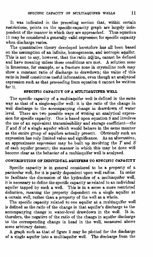
Hence, the specific capacity of the well is the algebraic sum of the specific capacities of the individual aquifers. If the specific-capacity graphs for the well and for each aquifer are plotted on the same set of axes, as in figure 4, the slope of the well graph must be the sum of the slopes of the aquifer graphs. Figure 4 represents the plot of data from a two-aquifer well.

With reference to equations 12 and 14, an analytical expression for the specific capacity of the well of figure 4 may be written as follows :

23 2 25T twhere Bn=. 'T log 2ere > in which Tn and S* are the coefficients of

e rw o w


600

500

400

300

200

100

100

\

AQUIFER 2

i i i i

.AQUIFER 1

i i ii

Static (nonpumping) head

I I I I I I II15 20 25 30

HEAD (h), IN FEET ABOVE ARBITRARY DATUM35 40

FIGURE 4. Composite specific-capacity graph for test well for pumping times of 1 hour. The head values in this figure are referred to an arbitrary datum 50 feet below the top of the well casing.

transmissibility and storage of the aquifer in question, and where Cn' is the entrance-loss coefficient of the particular aquifer.

The graph of figure 4 is useful in illustrating in general the perform ance of a multiaquifer well. No significant time variations exist be tween the various points plotted in figure 4; in other words, for each plotted value of discharge the corresponding head value was observed when that rate of discharge had been in effect for 1 hour. Preparation of any graph similar to figure 4 should include notation of the time


period used for observing the head values to be plotted against the various discharge rates of the well and the individual aquifers.

For any head value in figure 4 the discharge of the well is the alge braic sum of the discharges of the individual aquifers. Over a certain range one of the aquifers acts as a thieving zone, and the well discharge is less than the total discharge of the yielding zone.

Figure 4 illustrates the fact that a multiaquifer well is in effect never truly static; the net discharge of the well is zero when hw h01 but this zero discharge is the algebraic sum of several aquifer dis charges. In figure 4 aquifer 1 is discharging an amount equal to the recharge to aquifer 2, when well discharge is zero. Figure 5 shows the flow directions and piezometric surfaces corresponding to this internal discharge; a cone of depression exists in the piezometric surface of aquifer 1, and a cone of impression (cone of elevation) in that of aquifer 2. No piezometric surface is shown for the lowermost sandstone, indicating that it is not a significant aquifer.

The magnitude and direction of the internal flow in a given well not being pumped depend upon the transmissibilities, storage coeffi cients, and hydrostatic heads of the aquifers involved. Upward flow is at least as common as the downward flow shown in figure 5.

For the well represented in figure 5 a system of equations describing the internal flow may be set up by applying equation 9 to each aquifer, by using on the left in each equation the difference between the current water level and the undisturbed head of the aquifer in question, and by adding the condition that at any time

Qi+Q2=0. (16)

The main difference between the internal discharge of a multiaquifer well when it is not pumped and its discharge during pumping is in the value of the right side of equation 16. Equation 9 still applies to each aquifer, but the sum of the discharges must be some nonzero constant or function of time. The sum usually will be essentially constant, and this is the basis for postulating a decreasing time derivative for the individual discharges. It is unlikely that rapid variations in the individual discharges will occur after the initial moments of pumping where the aquifers are adjusting to a constant total rate of discharge from the well.

The zero-discharge intercepts of the lines in figure 4 are points of special interest in that they approximate the static heads of the individual aquifers. Each line on the graph must be constructed through an initial point of reference, from which the changes in Qu and hw are measured. In the specific-capacity graph of a single- aquifer well (fig. 3) this reference point was taken at zero discharge


Land surface

Piezometric surface aquifer I"

Piezometric surface aquifer 2

Aquifer 1

Aquifer 2

Lowermost sandstone

FIGURE 5. Schematic diagram of conditions in test well not being pumped.


and the static head of the aquifer. In the graph for an individual aquifer in a multiaquifer well the reference must be taken at the static (nonpumping) head in the well and at whatever discharge the aquifer shows for this head. This "static" point has generally been reached through a long period of internal discharge. In order to construct a line whose intercept on the horizontal axis of the graph represents the true static head of the aquifer under study, pumping intervals of the same duration as the internal discharge would have to be employed, and this is clearly impractical.

It has already been pointed out in the discussion of the time de pendence of specific capacity that large differences in the time of pumping will cause relatively small differences in the ratio &Q/Ahw provided the times in question are both of reasonably large magnitude. The slope and, therefore, the zero-discharge intercept of the line drawn through data obtained in a test of relatively short duration will usually approach that of the line that would be drawn through data obtained by pumping for time intervals approaching the duration of internal flow. The zero-discharge intercept of the specific-capacity graph related to an individual aquifer is thus a good approximation of the static head of the aquifer, and the approximation is only slightly improved by extending the times of pumping.

METHOD OF PRESENTATION OF EXPERIMENTAL DATA

The specific-capacity data provided by the methods described in this paper can be presented most effectively in a graph such as that of figure 4. The practical value of such a graph is obvious: it provides the specific capacities and hydrostatic heads of the various aquifers and shows the drawdown ranges over which thieving occurs in the well. Such information can be of great use to the owner or consultant in planning the development of the well, or in planning the drilling and development of additional wells in the immediate vicinity.

In the review of theory it was indicated that several factors may influence the linearity of the specific-capacity graph; among these were mentioned time variation between points, excessive well entrance losses, or a general inapplicability of equation 6 where the effects of variable discharge are still appreciably different from those of constant discharge at the time of measurements. The graph checks itself to a certain extent against these errors; if the experimental points fall on a straight line, it may be assumed that these effects are negligible.

In some investigations considerations of time and cost may pro hibit the construction of individual graphs for each aquifer; then graphs may be constructed for the zones of greatest interest, and an "equivalent aquifer" may be postulated for all the remaining zones of the well. An equivalent aquifer is defined as a single aquifer which


would perform in exactly the same manner as the group of aquifers it represents, taken as a whole. The specific-capacity graph related to the equivalent aquifer bears the same relation to the graphs of the aquifers it represents as the graph for the well bears to those of the individual aquifers of the well.

DESCRIPTION OF FIELD TESTS AND CALCULATIONS

Field tests of the methods presented in this paper were made over a 3-day period in September 1958, by use of an abandoned oil well in Mercer County, Pa.

Electric logs of the well (fig. 6) were made prior to the actual testing; they included self-potential, single-point resistance, 16- and 64-inch normal-resistivity, temperature, fluid-resistivity, gamma-ray, and caliper logs. The logs showed the well to be typical of the abandoned oil wells in the area. A wooden plug had been placed in the borehole at a depth of 580 feet in an effort to prevent salt water from deeper sands from contaminating the fresh-water sands above. This effort was only partly successful, for the fluid-resistivity log shows salt water below about 500 feet. The resistivity logs also suggest that the lower sandstone contains salt water, but fortunately it did not yield this water to the well at the pumping rates employed in testing.

The upper and middle sandstones, referred to as the first and second aquifers respectively, belong to the Pottsville formation of Pennsyl- vanian age and are productive aquifers throughout a large area of western Pennsylvania. The two aquifers vary in thickness and locally may be represented entirely by shale that forms a barrier to the move ment of ground water. The pumping data presented in this section do not reflect any such hydrologic boundaries, but it is felt that with longer pumping time such boundaries would be discovered and would affect the linearity of the experimental data.

EQUIPMENT

The arrangement of equipment at the test well is shown schemati cally in figure 7. The well was pumped with a centrifugal pump capable of discharging a maximum of 115 gpm against a 20-foot suction head. Discharge was regulated with a globe valve and measured by noting the time taken to fill a calibrated 55-gallon drum.

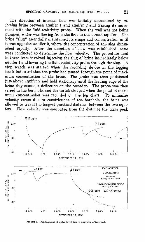
Water-level measurements to 0.01 foot were made frequently throughout the testing period, and drawdown data were obtained for all pumping rates. Figure 8 shows the prepumping levels, drawdown during pumping, and recovery trends after pumping.

Velocities of internal flow in the well between the aquifer 1 and aquifer 2 and between the second and third aquifers were measured by injecting brine into the flow at a selected depth through a K-i

SPECIFIC CAPACITY OF MULTIAQUIFEF WELLS 19

LU «i " I

QO

5 §

_w o ??. o

>y« n

IlII-ii

r -cZLJL


Valve Pump Brine Logging truck

Aquifer 2

Ohm-meters

FIGURE 7. Schematic diagram of equipment at test well, showing brine-tracing procedure.

plastic hose connected to a 15-gallon surface reservoir, and by tracing the movement of the brine with a fluid-resistivity electrode positioned from the logging truck. The fluid-resistivity apparatus contained in the truck included the measuring probe, a cable for lowering the probe into the well, a calibrated reel over which the cable passed so that the depth of the electrode was known at all times, and a device that continuously recorded the resistivity data against depth.

EXPERIMENTAL PROCEDURE

Information was obtained for several well-discharge rates relating the discharge of the individual aquifers to the drawdown of the well. As mentioned previously, the lower sandstone did not yield water to the well and therefore is not discussed.


The direction of internal flow was initially determined by in jecting brine between aquifer 1 and aquifer 2 and tracing its move ment with the fluid-resistivity probe. When the well was not being pumped, water was flowing from the first to the second aquifer. The brine "slug" essentially maintained its shape and concentration until it was opposite aquifer 2, where the concentration of the slug dimin ished rapidly. After the direction of flow was established, tests were conducted to determine the flow velocity. The procedure used in these tests involved injecting the slug of brine immediately below aquifer 1 and lowering the fluid resistivity probe through the slug. A stop watch was started when the recording device in the logging truck indicated that the probe had passed through the point of maxi mum concentration of the brine. The probe was then positioned just above aquifer 2 and held stationary until the leading edge of the brine slug caused a deflection on the recorder. The probe was then raised in the borehole, and the watch stopped when the point of maxi mum concentration was recorded on the log chart. To minimize velocity errors due to constrictions of the borehole, the brine was allowed to travel the longest practical distance between the two aqui fers. Flow velocity was computed from the distance the brine peak

11 a.m. 12 m. 1 p.m. 2 p.m. 3 p.m.

SEPTEMBER 17, 1958

4 p.m. 5 p.m.

32

2B

83 gpm EXPLANATION

Measured trend

Extrapolated trend

Irregular discharge during setting of valves

105 gpm (A0=22gpm)

11 a.m. 12 m. 1 p.m. 2 p.m. 3 p.m.

SEPTEMBER 18,1958

4 p.m. 5 p.m.

FIGURE 8. Fluctuations of water level due to pumping of test well.


traveled and the time taken for the brine to migrate from peak to peak. Figure 7 shows the operation. Discharge in cubic feet per minute was computed as the product of the flow velocity and the average area of the borehole (obtained from the caliper log) and was converted, for convenience, to gallons per minute.

The same procedure was employed for pumping rates of 22, 44, 72, 83, and 115 gpm. Measurements of water level were made prior to each period of pumping, and drawdowns were taken from the extrap olated trends of these measurements. During the 72-gpm dis charge the pump stalled after approximately 20 minutes; however, a measurement of internal discharge had been completed by this tune, and drawdown data were extrapolated to 1 hour in order to obtain the points for figure 4 corresponding to this pumping rate. All other pumping rates were maintained for at least an hour, and the data pre sented were taken for 1 hour of discharge. All pumping rates except that of 22 gpm followed a period of no pumping and were directly determined by measuring the time taken to fill a calibrated 55-gallon drum. The 22-gpm discharge was measured by increasing the well discharge from 83 to 105 gpm, for a net increase j0f 22 gpm. Draw down data corresponding to a discharge of 22 gpm were obtained by subtracting the extrapolated trend of the 83-gpm discharge from the measured water level during the 105-gpm pumping. Figure 8 sum marizes the measured and extrapolated drawdown and recovery trends for the various pumping rates.

TABLE 1. Summary of experimental data

Well discharge

Q» (gpm)

0 ....22*

44. .

72.........

83..

115... ..

Depth traveled by brine slug

(ft)

Max

57

63

60

59.

63

68

Min

55

62

58

56

62

66

Time interval

(min, sec)

4:00

5:42

4:53

4:37

5:04

6:05

Internal-flow velocity aquifer 1

to aquifer 2 (fpm)

Max

14.3

11.1

12.3

12.9

12.4

11.2

Min

13.8

10.9

11.9

12.2

12.2

10.9

Mean recharge

to aquifer 2'

(gpm)

58.0

'51.9

49.5

51.8

50.8

45.7

Total dis charge of aquifer 1

(gpm

58.0

»74.6

97.5

121.8

133.8

160.7

Change in head

Aft«, after Ihr

pumping (ft)

0.00»-.86

-1.50

-2.42

-2.72

-3.81

Head, A after 1 hr pump-»'

32.44

'31.58

30.94

30.02

29.72

28.63

i Computed by using borehole area of 0.55 square foot.> Values of h w obtained by adding values of Aft* to head of well at zero pump discharge, taken as 32.44 feet

above assumed datum which Is 50 feet below top of well casing.»Values obtained by taking differences between data for pump discharges of 83 gpm and 105 gpm, and

adding these differences to values for zero pump discharge.

Table 1 summarizes the discharge-drawdown data associated with 1 hour's pumping and shows for each rate of pumping the distance between the brine peaks, the time of traverse of the brine, the flow


velocity, the discharge or recharge of each of the two aquifers, the observed change hi the head hi the well, and the resultant head which is referred to an arbitrary datum 50 feet below the top of the well casing.

The data in table 1 concerning well discharge, aquifer discharge, and head are plotted on the composite specific-capacity graph hi figure 4.

PRESENTATION AND EVALUATION OF RESULTS

The head values plotted on figure 4 were obtained by adding algebraically the changes in head determined in the test to the static head of the well. Likewise, the internal-flow values on figure 4 were obtained by adding algebraically the observed changes in internal flow and the flow when the pump was shut down. Thus figure 4 illustrates the performance of the well after 1 hour of pumping, for situations in which the water level had recovered to about prepumping level. If pumping were to be started from a different initial point, as it may in a well showing seasonal fluctuations of water level, the slopes of the straight lines drawn in figure 4 would remain the same, but the lines would be displaced so as to pass through the new initial point.

The first aquifer gave the highest specific capacity, about 27 gpm per foot of drawdown. The second aquifer gave a specific capacity of about 3 gpm per foot of drawdown and acted as a thieving zone until relatively high pump discharges (about 500 gpm) were achieved. The zones below the second aquifer including the lower sandstone on the logs, and all zones beneath the plug exhibited no yield, either positive or negative, during the test, and consequently they were not included in the specific-capacity graph. When the water level in the well was essentially static, the upper aquifer discharged 58 gpm to the thieving aquifer.

Because of the extreme time difference between the 1-hour pumping interval and the internal-discharge span of several years, the zero- discharge intercepts of the lines for the two aquifers are only crude approximations of the static heads of these aquifers. These approxi mate static heads are summarized together with the specific-capacity data in table 2.

A somewhat better approximation of the static heads might be obtained by extrapolating the drawdown data to several years, on the assumption that the aquifer discharges would remain constant over that length of time, and by replotting the specific-capacity graph. This method gives a static head of roughly 20 feet below the arbitrary datum for the thieving aquifer and of 45 feet above datum for the upper aquifer. These results are open to serious question on the grounds that the measurements of internal flow were neither numerous


enough nor accurate enough to determine whether the two discharges were constant or were following trends. The linearity of the specific- capacity graphs suggests that the points are approximately those that would be attained by constant discharge. In general, however, more conclusive data on the time variation of the discharges should be obtained before large extrapolations are attempted.

TABLE 2. Data obtained from specific-capacity graph of figure 4

Aquifer 1__ , . _____ _________ ._ _, _ , , ____Aquifer 2 - , _ _ - ______._- -_ _ _Well.. _____________ - - - .-_ - -

Static head (ft above datum)

34 51632. 5

Specific capacity at 1 hr (gpm per

ft)

273

30

The greatest shortcoming of the analysis was clearly the limited accuracy of the method of measuring internal flow. Table 1 shows that many of the flow measurements have ranges of uncertainty of 2 or 3 gpm. (Each point of figure 4 represents the mean value of the range of uncertainty in that particular measurement.) The total variation in the internal flow over the entire test was about 12 gpm. A more accurate method of flow measurement is undoubtedly neces sary for work involving differences of this order. On an expanded scale the points on the lower graph of figure 4 all deviate from the line to some degree. The deviations are quite random, however, and although the straight line of figure 4 must be regarded as an approxi mation, it is certainly the best fit that can be made to the experimental data.

The authors felt that, for the measurement of downward flow, the brine-tracing method was somewhat more accurate than any of the other means at theu^disposal. A substantial improvement in accuracy might have resulted had a wider range of internal discharge been covered in the test, but the small capacity of the pump made this impossible.

CONCLUSIONS

Information on specific capacities, thieving, and hydrostatic heads of the various aquifers penetrated by a well can be of con siderable importance in the construction and operation of the well, or in the development of a well field. Although greater accuracy of flow measurement is desirable, the linear trend of the experimental data shows that the method is useful. As more refined techniques of flow measurement become available, it should be possible to achieve results of greater reliability with much less difficulty in fieldwork and calculation.

SPECIFIC CAPACITY OF MULTIAQUIFEE WELLS 25

LITERATURE CITED

Barbagelata, A,, 1928, Chemical-electric measurement of water: Am. Soc. CivilEngineers Proc,, v. 54, p, 789-802.

Bays, C.A., and Folk, S. H,, 1944, Geophysical logging of water wells in north eastern Illinois: Western Soc. Engineers Jour., v. 49, no. 3, p. 248-266.

Bird, J. M., and Dempsey, J. C., 1955, The use of radioactive tracer surveys inwater-injection wells: Kentucky Geol. Survey Spec. Pub. 8, p. 44-54.

Carslaw, H. S., and Jaeger, J. C., 1959, Conduction of heat in solids: London,Oxford Univ. Press, 2d ed.

Fiedler, A. G., 1928, The Au deep-well current meter and its use in the Roswellartesian basin, New Mexico: U.S. Geol. Survey Water-Supply Paper596-A, A, 24-32.

Jacob, C. E., 1950, Flow of ground water, in Rouse, Hunter, Engineering hydrau lics: New York, John Wiley and Sons, p. 321-386.

Jacob, C. E., and Lohman, S. W., 1952, Nonsteady flow to a well of constantdrawdown in an extensive aquifer: Am. Geophys. Union Traris., v. 33,no. 4, p. 559-569.

Jones, P. H , and Skibitzke, H. E., 1956, Subsurface geophysical methods inground-water hydrology, in Advances in geophysics, v. 3, p. 241-300: NewYork, Academic Press, Inc.

Meinzer, 0. E., 1928, Methods of exploring and repairing leaky artesian wells:U.S. Geol. Survey Water-Supply Paper 596-A, p 1-3,

Rorabaugh, M. I., 1953, Graphical and theoretical analysis of step-drawdown testof artesian well: Am. Soc. Civil Engineers Proc., v. 79, Separate 362, 23 p.

Skibitzke, H. E., 1955, Electronic flow meter: U.S. Patent No. 2,728,225. Theis, C. V., 1935, The relation between the lowering of the piezometric surface

and the rate and duration of discharge of a well using ground-water storage:Am. Geophys. Union Trans., pt. 2, p. 519-524.

o

U.S. GOVERNMENT PRINTING OFFICE: I960 O - 546681