boss competence and worker well-being€¦ · boss competence and worker well-being ... economics...

Warwick Economics Research Paper Series

Boss Competence and Worker Well-being Benjamin Artz, Amanda H Goodall & Andrew J Oswald

October, 2015 Series Number: 1072 ISSN 2059-4283 (online) ISSN 0083-7350 (print)

Forthcoming in ILRR

Boss Competence and Worker Well-being

Benjamin Artz, Amanda H Goodall, and Andrew J Oswald‡

September, 2015

Abstract

Nearly all workers have a supervisor or ‘boss’. Yet little is known about how bosses influence

the quality of employees’ lives. This study is a cautious attempt to provide new formal evidence.

First, it is shown that a boss’s technical competence is the single strongest predictor of a

worker’s job satisfaction. Second, it is demonstrated in longitudinal data -- after controlling for

fixed effects -- that even if a worker stays in the same job and workplace a rise in the

competence of a supervisor is associated with an improvement in the worker’s well-being.

Third, a variety of robustness checks, including tentative instrumental-variable results, are

reported. These findings, which draw on US and British data, contribute to an emerging

literature on the role of expert leaders in organizations. Finally, the paper discusses potential

weaknesses of existing evidence and necessary future research.

Keywords: bosses, expert leaders, leadership, job satisfaction, happiness.

JEL codes: I31, J28, M54

For their valuable suggestions, we would like to record our thanks to the editor, Peter Kuhn, and

three referees. For many helpful discussions, we are grateful to Marina Halac, John Heywood,

Lilian de Menezes, James Oswald, Andrea Prat, and Bert Van Landeghem.

‡ The authors’ affiliations are, respectively, University of Wisconsin at Oshkosh; Cass Business School, City

University London, and IZA; University of Warwick, CAGE Research Centre and IZA.

2

1. Introduction

Although bosses are ubiquitous in modern society, there has been almost no research by

industrial relations researchers and labor economists into how bosses affect the happiness and

well-being of the workers they oversee.1 This paper cautiously offers new evidence. It suggests

that the underlying technical competence of a boss may have major consequences for workers’

job satisfaction. A range of correlational findings are presented. The paper draws upon cross-

sections and panels; it uses data on job satisfaction from the United States and Britain; it reports

seven different forms of evidence. Although the paper’s evidence is of a simple kind, and cannot

have the persuasiveness of a perfect randomized controlled trial, we hope the later patterns and

results might interest many different types of researcher. Job satisfaction is an indicator of

worker well-being and is known to be a predictor of quit rates (recent work includes Clark 2001

and Levy-Garboua et al. 2007). Figure 1 gives an immediate non-technical flavor of the

potential significance of supervisor competence. The paper’s main findings, which appear to be

the first of their kind, are reported in Tables 2 to 7, and in an Appendix.

This study is able to examine changes in supervisor ‘within person and firm’ (and thus

relates to work on social capital in the workplace such as Helliwell and Huang 2010, the

economics of hierarchies such as Garicano 2000, managerial attention such as Halac and Prat

2014, and on so-called expert leaders such as Goodall, Kahn and Oswald 2011). The paper also

attempts to consider issues of causality. While it cannot resolve all the difficulties, the paper

investigates a longitudinal sample of workplaces in which the identity of the employee remains

the same and the only change is in the quality of the supervisor (and the paper also tentatively

provides some instrumental-variable estimates). A significant role is found for variables that

have been little-studied by labor researchers, such as:

whether the supervisor worked his or her way up inside the company

1 A search through the standard labor textbook Filer, Hamermesh and Rees (1996), for example, finds only one

mention of the word ‘boss’ or ‘supervisor’ in its 600 pages; a text such as Ehrenberg and Smith (2012) has a larger

number of mentions but does not provide an analytical model or discuss data. As another illustration, a search on

the Web of Science shows that in the whole history of the Journal of Labor Economics there is only one article that

mentions, in its Key Words or Abstract or Title, the word “supervisors” and one other article that mentions “bosses”.

The same is true of the Journal of Human Resources. The Industrial & Labor Relations Review has a number of

articles, the closest in spirit perhaps being Heywood et al. (2002), but none looks at links with job satisfaction. In

the Journal of Occupational and Organizational Psychology, the closest paper to ours appears to be Miles et al.

(1996), but that paper does not make the same point as ours and is instead about supervisors’ communication. There

are large and important related literatures on procedural justice, by McFarlin and Sweeney (1992) and others, and on

citizenship by authors such as Capelli and Rogovsky (1998), and on group-payment systems (by Freeman et al. 2008

and Green and Heywood 2010) but these also do not cover the issue tackled here.

3

whether the supervisor could in an emergency do the employee’s job

the supervisor’s assessed level of competence.

The first two of these are, in principle, indirect indicators of supervisor competence, but they also

seem of independent interest as variables that are rarely examined by labor-market researchers.

This paper follows in the footsteps of Freeman (1978) and Lazear, Shaw and Stanton

(2011). It links to a recent literature that -- though not directly on the influence of bosses upon

well-being -- seeks to understand the influence of bosses upon productivity. Prominent among

this recent literature are writings such as Branch, Hanushek and Rivkin (2013) and Lazear, Shaw

and Stanton (2011) itself. The paper’s results are also consistent with new evidence in Brown et

al. (2014) on links between employee trust (in managers) and good workplace outcomes. More

broadly, this study fits within a growing well-being research literature written by economists and

psychologists (including Benjamin et al. 2012, Booth and van Ours 2008; Clark and Oswald

1996, Diener et al. 1999, Di Tella et al. 2001, Easterlin 2003, Frey and Stutzer 2002, Graham

2011, Hamermesh 2001, Layard 2006, Powdthavee 2010, and Senik 2004).

Although the happiness and job satisfaction of workers might be believed to matter

strongly in itself, it is now thought that it also does so indirectly. There is growing evidence that

‘happier’ workers are more productive (in the work of Carol Graham, such as Graham et al.

2004; many papers by the late Alice Isen; and research by Bockerman and Ilmakunnas, 2012;

Edmans 2012; De Neve and Oswald 2012, and Oswald, Proto and Sgroi 2015). The broader

background is a more general research effort into the effects of leaders upon measures of

organizational performance. One strand, to which this paper contributes, attempts to understand

the role of so-called ‘expert leaders’ (Goodall 2009, 2011). Such research has largely been at a

senior level: it has attempted to separate CEO effects from industry or firm effects in order to

calculate the explanatory power of leaders and their characteristics (e.g. Thomas 1988;

Finkelstein & Hambrick, 1996; Waldman & Yammarino 1999; Souder, Simsek & Johnson,

2012; Dezso & Ross, 2012; Bloom et al. 2012). There is a literature on high-involvement

management (Guthrie 2001, Bryson et al. 2005, Bockerman et al. 2012, Boxall & Macky 2014),

but that has not tackled the exact issue considered in this paper, and on the influence of private

equity (Agrawal & Tambe 2014).

4

Why would supervisors matter? There is no standard theory of how a supervisor2 affects

a workplace. Our approach has been influenced by the innovative work of Lazear et al. (2011),

which discusses the potential training, advising, and motivating functions of bosses. That

channel is logical and almost certainly captures some of the activities of real-world bosses and

supervisors (Becker and Wrisberg 2008 and Goodall et al. 2011 contain some discussion of this

for an elite sports setting). Nevertheless, our conception differs in one way. Bosses are, in

principle, special workers because they are in charge. They make a range of organizational

decisions. Therefore, it may be desirable not to view a boss as just another factor of production,

or as altering only the quality of an employee’s input through greater marginal product in the

production function. Instead, it may be appropriate to view a boss as being able to shape the

nature of the organization.

This paper is designed as an empirical rather than theoretical contribution. However, as

one approach to possible thinking, we describe below a characterization of equilibria of different

kinds of efficiency, and how supervisors might alter the outcome from one such equilibrium to

another. We implicitly have in mind a wider set of supervisory functions than in Lazear et al

(2011). One important conceptual challenge, on which our paper will be silent, is that real-world

employees and supervisors are sorted into subtly different kinds of firms and specific job tasks; a

weakness of our theoretical account will be that it ignores much of such heterogeneity.

Consider a world in which there are three kinds of agents to be understood – the worker,

the supervisor, and the employer (ie. the firm or organization). Imagine that a worker and a

supervisor can be thought of as combining in their efforts to produce some kind of output. For

analytical simplicity, assume that the firm can be thought of as existing in the background rather

than the foreground, but that this employing firm has, ultimately, to receive a share of whatever

is produced jointly by the worker and the supervisor. The worker and the supervisor must then

decide how to behave. Let the worker take some kind of action, denoted a. Let the supervisor’s

action be denoted s. These could be thought of as effort levels but can also be viewed much

more broadly (s could be advice given to a worker by an experienced supervisor, for example).

The variables a and s can easily be generalized to vectors of actions; but in the algebra below, for

2 This might sound paradoxical, as supervisors are all around us, but historically the implicit presumption coming

from labor economics has been that it is possible to treat supervisors (where it has done so explicitly at all) as just

another kind of input in the F(...) function.

5

simplicity, they will not be. They will instead be viewed as single variables defined on the real

line. Together, the two actions lead to output Q for the firm:

Q = q(a, s). Firm’s output (1)

where both a and s contribute to output and have positive first-derivatives. Something has also

to be assumed about incomes. Assume that the worker gets a share psi, ψ, of the output while

the supervisor gets share sigma, σ. The remainder goes to the employer.

Assume the employee’s utility function takes the general form

µ = µ(a, s, ψQ) – c(a) Worker’s utility (2)

where part of utility thus depends directly on the actions a and s, another part depends on the

share of the output that accrues to the worker, and a final part depends on the cost of action a,

which is assumed to be captured by a convex increasing function c(a). At this stage, no

assumption needs to be made about the sign of the derivatives of the µ function in equation (2).

For simplicity, the cost function is treated in the above formulation as separable, but that can

straightforwardly be dropped. If desired, µ here might be thought of approximately as the

‘overall job-satisfaction’ of a worker. It is a measure of the total utility from the work

environment.

Finally, write the supervisor’s utility function in a symmetric way. It is therefore

ʋ = ʋ(a, s, σQ) – k(s) Supervisor’s utility (3)

where in this case the function k(s) captures the supervisor’s cost of action. For ease of notation,

the form of equation (2) and (3) can be written in a more compressed way. Define identities

µ(a, s, ψQ) = u(a, s) (4)

ʋ(a, s, σQ) = v(a, s). (5)

Hence, from these, write the two parties’ net utilities as:

Worker’s utility = u(a, s) – c(a) (6)

Supervisor’s utility = v(a, s) – k(s). (7)

This framework is a very simple one, but it is allows us to think of the different types of

outcomes that might be expected to occur. Put more generally, simultaneous-move ‘public

goods’ games with complementarities in the production function are known have multiple

equilibria in a wide range of cases, and this kind of conceptual background therefore offers one

6

potential way of thinking about 'what supervisors do'. Both communication and co-ordination

(changing the order of moves) are ways that supervisors might perhaps increase the chances that

better equilibria are reached. For earlier discussions of such ideas, see the interesting work of

Brandts and Cooper (2007) and Goerg et al. (2010). As Brandts and Cooper (2007) put it: “in

the absence of managerial intervention, subjects invariably slip into coordination failure…we

find that communication is a more effective tool than incentive changes for leading organizations

out of performance traps.”

Consider initially what might be called the inexpert-supervisor case: here there is a

supervisor who is relatively inexperienced in the nature of the work and the type of workplace.

He or she thus lacks deep knowledge about the worker and environment. Assume that the

supervisor is able to observe the action of the worker, but beyond that understands little about the

work-setting. In this case, because the supervisor is so inexpert, the two parties can be thought

of as behaving in a non-cooperative rather than cooperative way. There is then potentially a

Nash equilibrium where both the worker and the supervisor choose their actions (a, s)

independently. This outcome is characterized by the usual first-order conditions

a) = 0 (8)

and

s) = 0 (9)

so the outcome, which can be thought of as the intersection of two reaction functions, is, for the

standard reasons, either strictly or weakly sup-optimal for the worker-supervisor pair (intuitively,

because each ignores the externalities imposed on the other party). Equations (8) and (9) define

a self-reinforcing fixed point and thus one kind of equilibrium.

It might be thought that the supervisor in the above set-up is behaving foolishly.

However, that reaction would not be an appropriate one. This kind of non-cooperative outcome

is a feasible and rational one for a supervisor who has limited knowledge. It requires only that

(i) the supervisor knows his or her own preferences, and (ii) the supervisor be able to see the

action chosen by the employee, even if the supervisor has little understanding of why the worker

is choosing that action or how the workplace could be organized better.

Some supervisors, however, may be different: call them expert supervisors. They are

individuals who have a deep and expert knowledge of both the core business and the nature of

the worker. In such a case, an ‘expert supervisor’ could, in principle, help guide the pair to a

7

jointly efficient outcome (for the pair, and, by implication, for the employing firm in the

background). This is not a minor variant on the previous outcome. Instead, the outcome is not a

Nash equilibrium, but rather the expert supervisor helps to produce a cooperative equilibrium.

The worker and the supervisor choose actions (a, s) jointly to solve

Maximize u(a, s) – c (a, s) s.t. v(a, s) - k ≥ V

where V is an arbitrarily fixed level of net utility for the supervisor. Thus this case is

characterized by Pareto-efficiency and:

a) = 0 (10)

and

s) = 0 (11)

where is the usual Lagrangean multiplier.

The defining aspect -- and perhaps ultimately a testable one -- here is that the ‘expert

supervisor’ has to have an experienced understanding of the work setting and the character of the

employees. The reason is simple. Such information is essential to achieve a cooperative

equilibrium, whether by implicit negotiation or explicit negotiation. The expert supervisor leads

the pair away from inefficient Nash equilibria. As can be seen, equations such as (10) and (11)

satisfy the requirements for Pareto efficiency. The worker and the supervisor will thus typically

have higher utilities in this case. ‘Expert bosses’ can offer workers the best outcomes. By

contrast, to get to a Nash equilibrium in case 1, it is not necessary to know (almost) anything

about the other side's preferences. An agent simply maximizes given what he or she sees the

other side choose as the opposing side’s action.

By such logic, workers can benefit from an expert supervisor, and not merely from any

higher income level that such a supervisor might make possible. Supervisors’ deep expertise

may act to alter, and improve, the very nature of equilibrium outcomes. This paper does not

attempt, and because of its type of data is unable, to test a narrow form of this framework, but

this conception offers a potential way to think about the later empirical issues.

2. Cross-sectional data

8

The data used3

here are drawn from (i) a single cross-section from the National

Longitudinal Survey of Youth in year 1990, (ii) a cross-section from the Working in Britain

Survey in year 2000, and (iii) then a set of panel data from the NLSY for a range of years

between 1979 and 1988. These data sets are statistically representative of their chosen

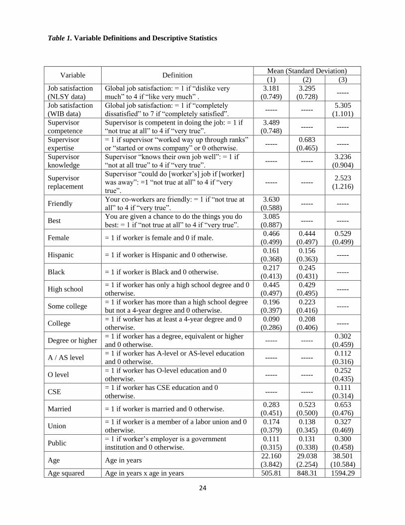
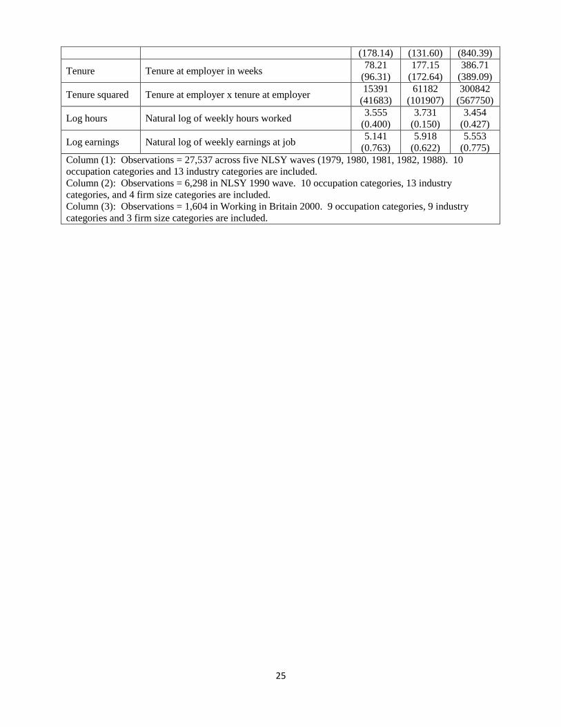
populations. Table 1 describes their key features; it reports means and standard deviations.

Elementary evidence consistent with the possible importance of supervisors is visible in

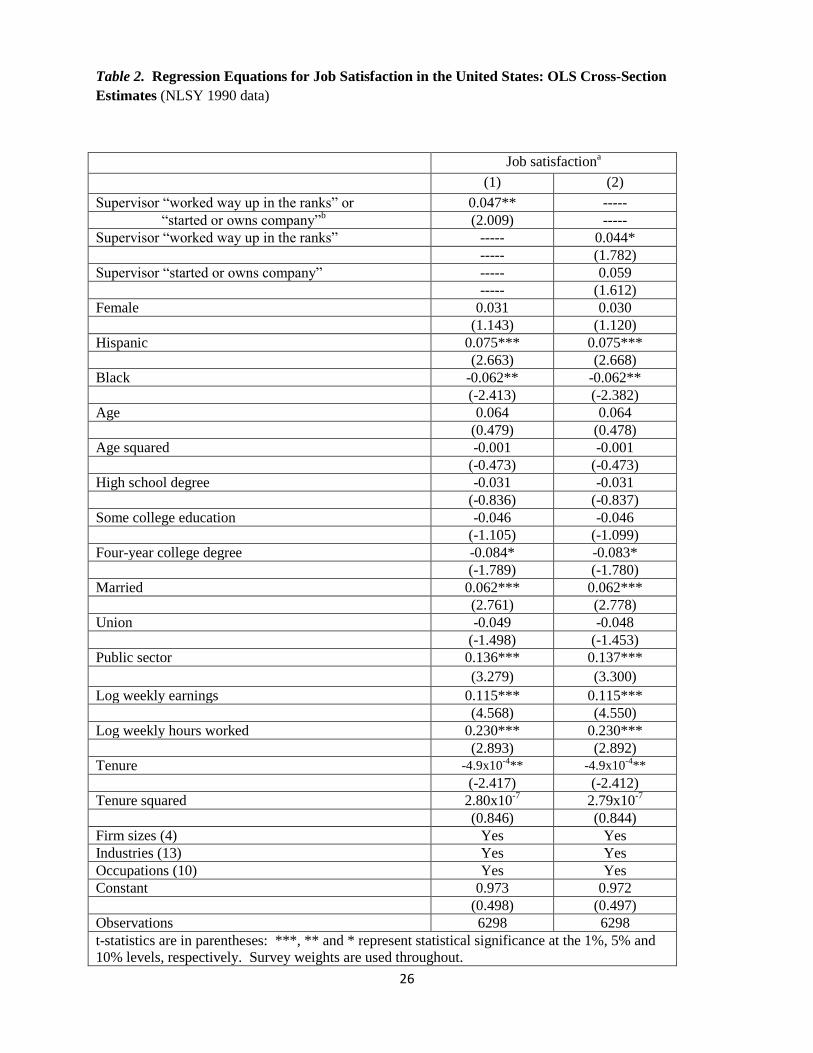
the regression equations of Table 2. Here the dependent variable is a measure of the job

satisfaction4 of approximately 6000 randomly sampled young US workers, where answers are on

a 4-point scale and the wording is “Overall, how satisfied are you with your job? I like it very

much, …., I dislike it very much.” [the foot of Table 2 gives full wordings]. For ease of reading,

we report findings with a simple OLS estimator. However, the results are essentially unaffected

by using instead an ordered estimator; those versions of the equations are available upon request.

The mean of the dependent variable in Table 2 is approximately 3.2 on a 4-point scale. It has a

standard deviation (driven by the across-person variation) of approximately 0.7.

We are interested in the consequences of highly competent, or ‘expert’, supervisors.

There is no single or conventional way to define competence. Hence in this paper we examine a

number of different measures.

In Table 2, a dummy variable for the supervisor having worked his or her way up the

ranks is used, and another for the supervisor having started or owns the company. After

adjusting for a conventional set of covariates, a dummy variable for these two together (a form of

either-or dummy) enters, in column 1 of Table 2, with a positive coefficient of 0.047. This

coefficient is significantly different from zero at the 95% level on a two-tailed test. It is

substantial.

To get a sense for the estimated effect-size, some standard of comparison is required. A

natural approach is to examine the coefficient on supervisor-competence variables against the

coefficients on other variables in a regression equation.

3 Most surveys do not report information about the role of supervisors, so we have to use selected years for which

data are available. 4 Most of the results in the paper use job-satisfaction numbers as the worker well-being variable. But we have

replicated the spirit of these results, and the key finding remains the same, with alternative measures (such as desire-

to-quit information in the WIB dataset, and satisfaction with supervisor). Those equations are available on request.

9

Comparing, for example, to famously large coefficients in the job-satisfaction literature,

the number 0.047 is close to being the same size as the coefficient on marriage, and

approximately one third of the size of the extra satisfaction associated with working in the public

sector. Other variables enter in ways familiar from the literature. For example, after controlling

for income, those with higher levels of education are less satisfied with their jobs (one of the

early demonstrations was in Clark and Oswald 1996), the level of earnings enters positively, and

black workers suffer a negative coefficient. The second column of Table 2 explores the effects

of dividing the supervisor dummy variable into its two constituent parts. Here the two

coefficients (0.044 and 0.059 respectively) are close in size, although, as might be expected after

the reduction in statistical power, the individual t-statistics become weaker at approximately 1.8

and 1.6.

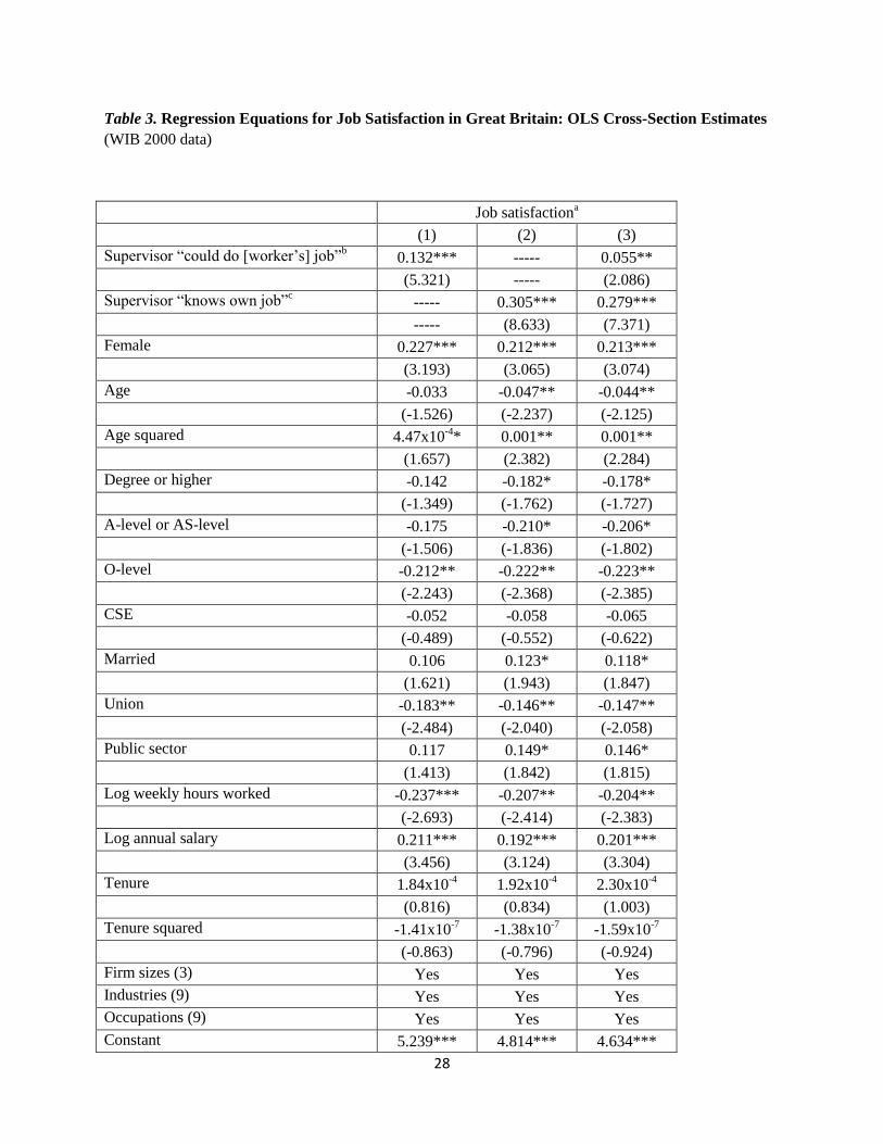
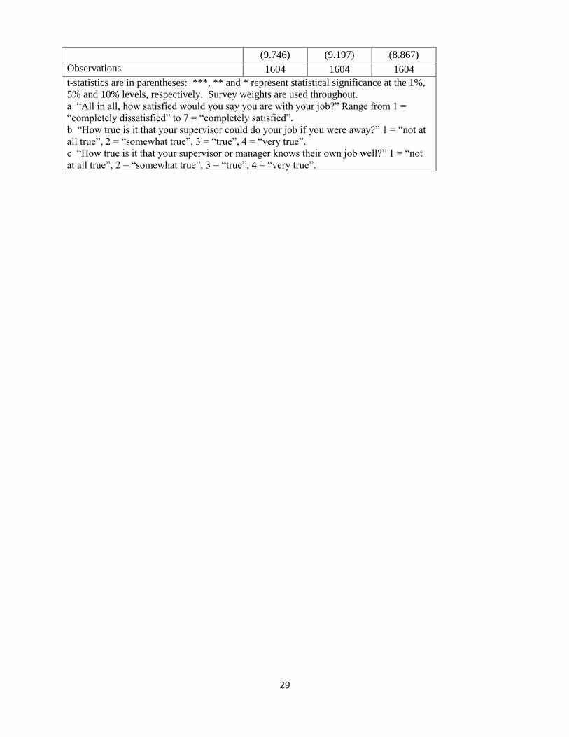
Table 3 is in the same spirit but uses a British data set, the WIB 2000. This provides a

randomly selected sample of approximately 1600 individuals. Here the wording used to

construct the dependent variable is similar to before but workers now answer on a 7-point scale

from “I am completely satisfied,….I am completely dissatisfied.” The mean of the dependent

variable in Table 3 is approximately 5.3, with a standard deviation of approximately 1.1.

In Table 3, workers are asked “Could your supervisor do your job if you were away?”

and also “Does the supervisor know their own job well?” Both of these allow the construction of

a banded dummy variable for competence. This is because they are coded on a 4-point scale

from “Yes, very true” to “No, not true at all”. In the first case, the mean of workers’ answers is

2.5 and in the second case it is 3.2 (apparently a large number of workers do not believe the

supervisor could fill in for the worker if the worker were away, whereas supervisors are given

higher grades for the ability to do their supervisory role).

It might reasonably be argued that different interpretations are possible. Nevertheless,

they seem independently interesting and apparently have not been studied before.

The coefficient in Table 3 on the variable denoted ‘supervisor could do the worker’s job’

is positive, large, and statistically well-determined. It is estimated at approximately 0.13 with a

t-statistic in excess of 5. Employees enjoy their jobs far more where the supervisor is assessed as

technically competent. To get a sense of the size of the coefficient, it is necessary to note that

the variable here runs from a value of 1 to a value of 4. Hence a movement from Not True at All

(that the supervisor could do the person’s job) to Very True would be associated with a

10

quadrupling of the level of job satisfaction from this source. The first column of Table 3

therefore points to a striking pattern in the data. Here the existence of a highly competent

supervisor would imply 0.4 extra points (on a seven-point scale) on the worker’s job satisfaction.

This is almost double the combined coefficients of marriage and working-in-the-public-sector.

We return later to what might account for this strength.

Columns 2 and 3 of Table 3 report coefficients on a variable that codes answers to the

question “How true is it that your supervisor or manager knows their own job well?” As a

referee has pointed out, because of its directness this question might be thought to have special

appeal. In column 2, the coefficient on this variable is 0.305 with a t-statistic greater than 8. The

values of the variable run from 1 to 4. Thus a statistically representative worker whose

supervisor knows his or her own job very well is markedly more contented than other workers.

The difference in job satisfaction is approximately 1 full point on a seven point scale. Column 3

of Table 3 shows that both of these independent variables, for ‘supervisor could do my job’ and

‘supervisor knows own job well’, are significant when entered together in the specification. As

would be expected, the individual coefficients in column 3 are slightly lower, at 0.055 and 0.279

respectively, than in the previous two columns.

3. Pooled equations and longitudinal evidence

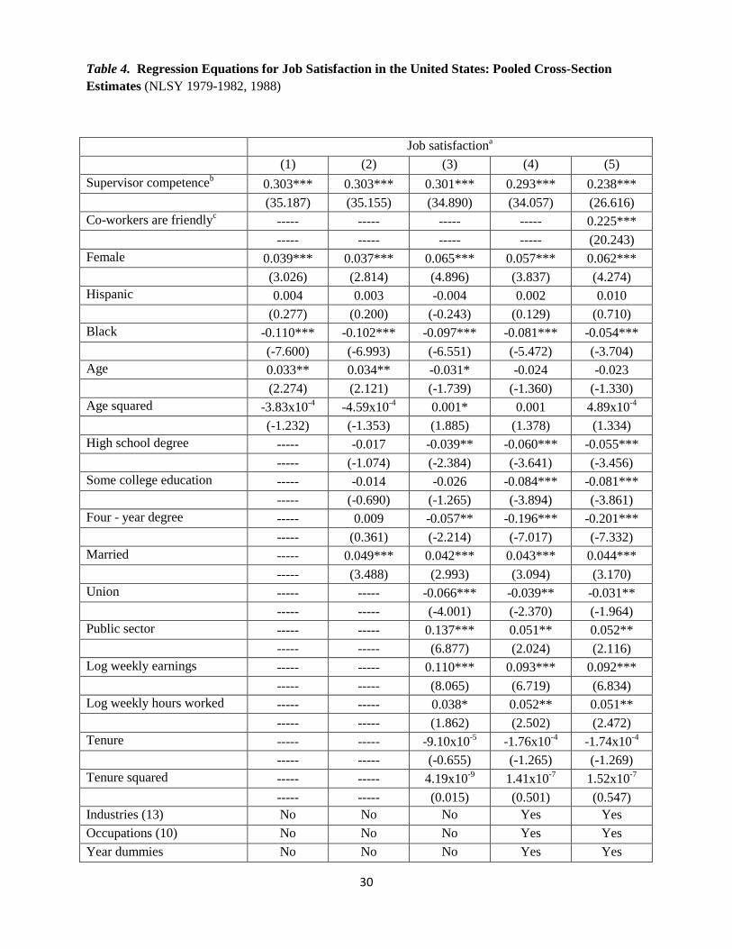
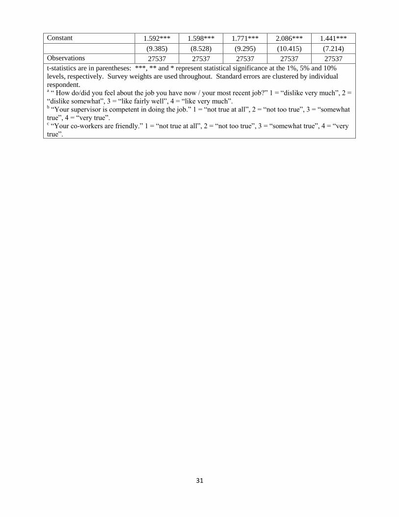
Table 4 contains evidence on a larger data set. It gives pooled cross-sectional estimates

from the NLSY for the years 1979, 1980, 1981, 1982, and 1988. Here we have used all of the

years in which a particular supervisor question was included in the survey, namely, “Is your

supervisor competent in doing the job?” where people may answer on a 4-point scale “Not true at

all, …., Very true”. The sample size in these regression equations is approximately 27,000

employees.

The coefficients on the supervisor variable are now very substantial. In the first column

of the job satisfaction equations of Table 4, for example, the estimated coefficient is 0.303 with a

t-statistic of approximately 35. This implies that a movement from having the least-competent

category of supervisor to the most-competent category of supervisor would be associated with a

difference in job satisfaction of nearly 1 full point on a 4-point scale.

In column 1 of Table 4, we exclude a large number of the potentially relevant influences

on the job satisfaction of the workers who are being supervised. Later columns gradually

introduce more and more of those. Only minor changes are observed in the estimated coefficient

11

on the supervisor-competence variable. By the fourth column of Table 4, the coefficient is still

approximately 0.3.

A coherent objection to Table’s 4 estimates is that they are biased because of the fact that

the personality of the worker is here an omitted variable. Hence it might be that inherently

‘cheerful’ people tend both to report high levels of job satisfaction and to give favorable

assessments of their supervisor (they simply have a sunny outlook about everything). In that

case, the association between the worker’s well-being and the assessment of the supervisor might

be spurious. One way to probe this possibility is to include another variable for the inherent

cheerfulness of the employee, and to see whether that largely eliminates the significance of the

supervisor variable. The final column of Table 4 does so. It includes a variable for whether the

individual reports that his or her co-workers are friendly. The friendliness variable is positive in

column 5 of Table 4. Once this inclusion is done, the coefficient on the supervisor-competence

variable is barely affected. It falls by only approximately 0.05 points to 0.238. This result is

consistent with the existence of a genuine role for supervisor competence.

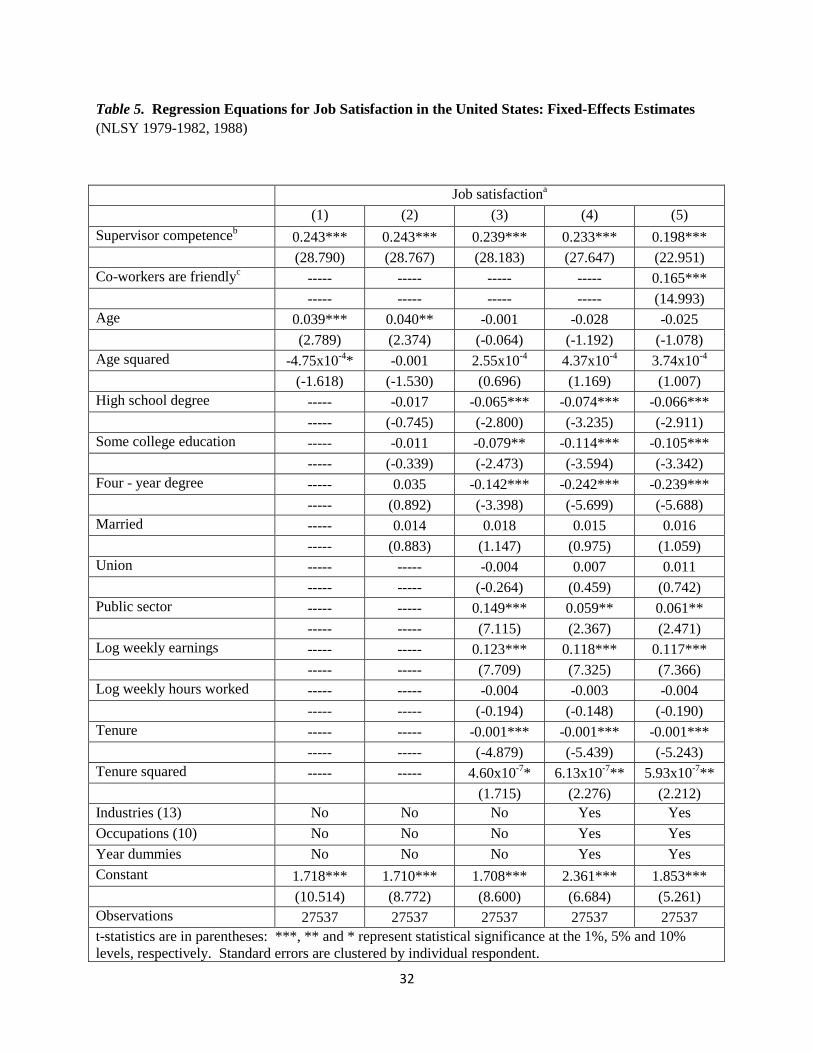
Table 5 reports another form of evidence. In these fixed-effects regression equations, we

are able to confirm that the positive correlation between job satisfaction and a supervisor-

competence variable is not spuriously due merely to factors such as omitted personality factors.

Table 5 continues to give similar results to those earlier tables, which establishes that such an

interpretation cannot explain the patterns in the data.

Once again, consecutive columns of Table 5 build up to fuller specifications. The

supervisor coefficient remains highly stable, at approximately 0.23, across the first four columns

of the table. That is not far from the estimate size from cross-sectional estimates. This fact itself

suggests there is comparatively little bias from omitted person fixed effects in cross-sectional

equations. Once again, the addition of the ‘co-workers are friendly’ variable has only a minor

effect on the supervisor coefficient, and itself is positive and well-determined (which is arguably

suggestive, because this is in a fixed-effects equation, of the idea that the friendliness of co-

workers genuinely matters). In column 5 of Table 5, the variable for supervisor competence

remains at approximately 0.2 with a t-statistic of approximately 23.

The other variables in these fixed-effects specifications of Table 5 are of interest. Even

in the fullest specification, there is evidence that job satisfaction depends upon education,

12

whether the person works in the public sector, weekly earnings, and tenure. These variables’

coefficients are necessarily estimated from the ‘switchers’ in the data set.

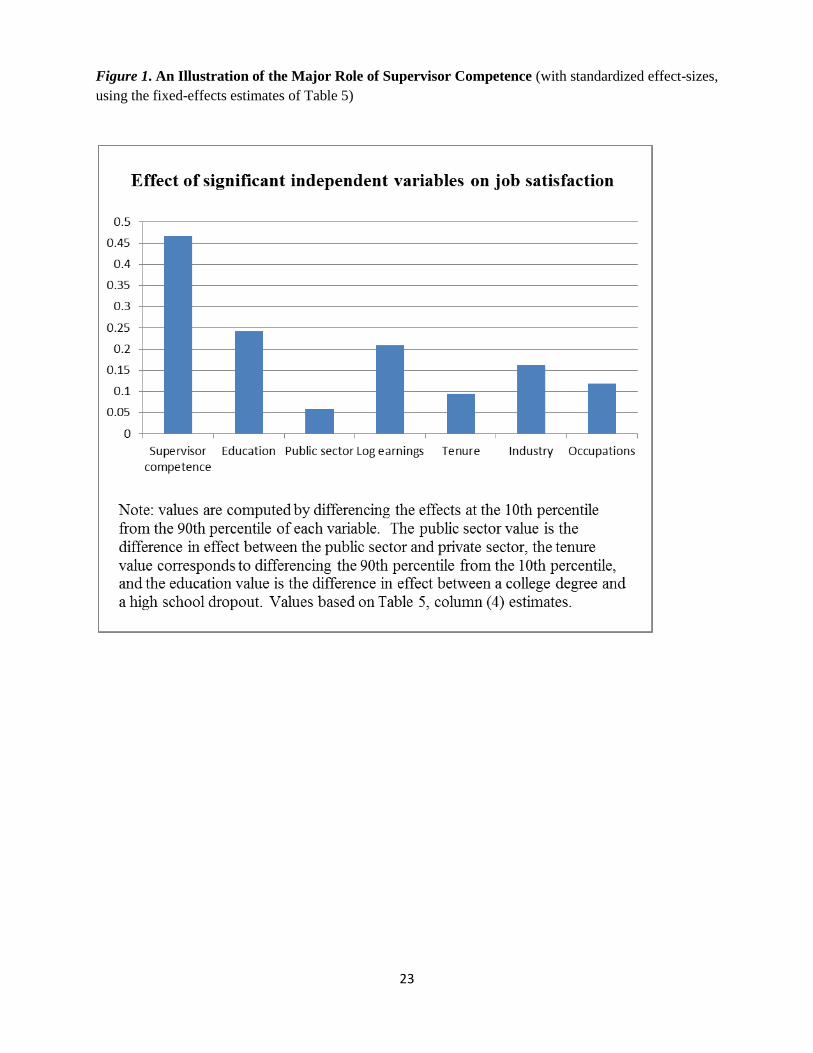
An illustration of effect-sizes is provided in the histogram of Figure 1. Here it is

necessary to standardize the data in some way, so that the quantitative role of different

explanatory variables can be compared appropriately. We do so here by using 90th

percentile –

10th

percentile movements in the main independent variables (except, necessarily, in the case of

the zero-one public-sector dummy variable). The size of the estimated supervisor effect, in the

first column of Figure 1, is strikingly large. It dominates any of the more conventional

influences upon people’s job satisfaction, including the role of worker remuneration5. Here the

10th

percentile for the supervision variable is the second-lowest rating of supervisor competence;

the 90th

percentile is the highest of the four possible ratings; thus this change corresponds to a 2-

point movement in the independent variable that measures supervisor competence.

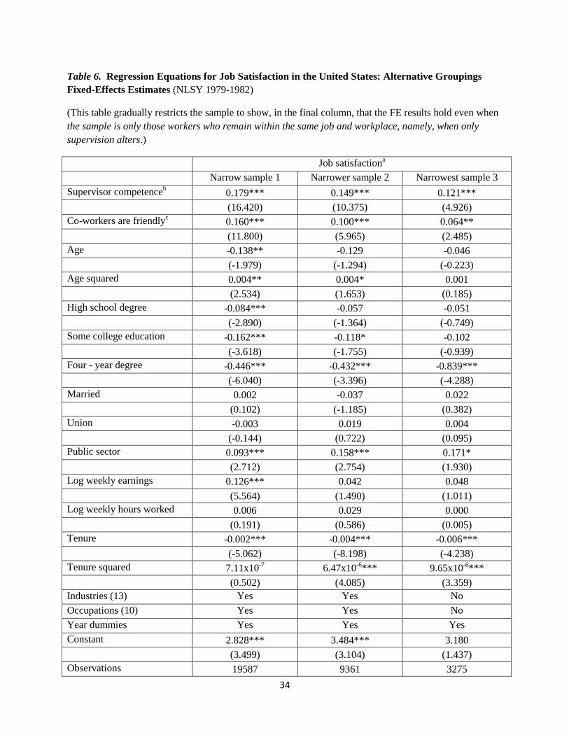
Table 6 reveals that the paper’s principal finding is robust to an important form of

correction. A potential objection to the previous table, Table 5, is that in the whole sample used

there, the switchers might be moving disproportionately to different workplaces with

(unobservably) better characteristics, and that this, it might be argued, could lead to an upward

bias on the coefficient on the supervisor-competence variable. We show that this is not what is

driving the paper’s key finding. Columns 1 to 3 of Table 6 reveal that even in the final column,

where we study only those who remain in the same job and same workplace, we again find an

influential role for the supervision variable. As would be expected, the coefficient is slightly

lower, at 0.121. It remains well-determined, with a t-statistic of approximately 5.

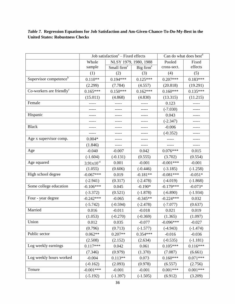
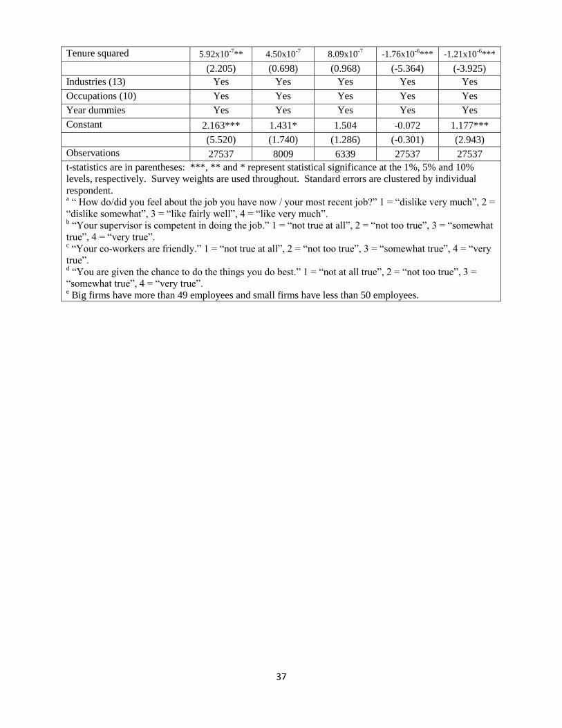
Are some kinds of employees more sensitive to bosses’ actions? What of certain kinds of

workplaces? Further robustness checks are reported in Table 7. Column 1 tests for an

interaction between the age of the worker and a variable for supervisor competence. The level of

supervisor competence continues to be highly significant. An interaction term, however, enters

with a coefficient of 0.004 and a t-statistic of approximately 2.3. This implies that the marginal

effect of supervisor competence on the job satisfaction of the worker is considerably larger for

older employees. One possible interpretation of this is that young workers are highly mobile and 5 A referee has asked us for a back-of-the-envelope calculation of the required monetary ‘compensating variation’

for having a much poorer supervisor. That number is large. Although we would wish to view this kind of

calculation as illustrative rather than as causal, the arithmetical answer, taking Table 5’s estimates, is that around the

mean of earnings a one standard-deviation worsening of supervisor competence (admittedly a substantial worsening)

would have to be offset by approximately a 150% change in the worker’s pay. This conclusion, and the largeness of

the estimate, is consistent with the spirit of the ideas of Brandts and Cooper (2007).

13

thus less susceptible to good or bad supervisors; another is that the old hold more senior

positions in the job hierarchy and that their bosses are therefore fewer and individually more

influential. It is then shown, in columns 2 to 3 of Table 7, that in a fixed-effects job satisfaction

equation a supervisor-competence variable works powerfully both for the large establishments

and the small establishments (where the cut-off chosen for the definition of smallness is having

fewer than 50 employees). Its coefficient is slightly greater in column 2 for the group of small

establishments. In each of the two columns its t-statistic exceeds 5. Columns 4 and 5 of Table 7

alter the dependent variable. They use not a job satisfaction variable but instead a variable for

how the worker answers: “You are given the chance to do the things you do best? Not true at

all,….Very true”. The aim is to probe whether supervisors might have effects through such a

channel. The coefficients on the supervisor competence variable are then, respectively, 0.207

and 0.183. Hence these findings are consistent with such a view. Competent supervisors may

assign their workers particularly effectively. Further issues related to the gender of bosses are

taken up in Artz and Taengnoi (2014); we do not pursue those here.

4. Further issues

There remain a number of issues and concerns; given length constraints, we briefly

review them below.

Issue 1: Although it is true that the results cannot be explained by omitted fixed-effects, they

could, in principle, be the spurious result of exogenous mood swings. Consider a worker who

becomes ‘happier’ for some external reason. Then he or she might see the world as a rosier

place, and thus both report higher levels of job satisfaction and also view the supervisor more

favorably.

However, such a criticism, while a cogent one, cannot account for all of the paper’s findings. It

is unable to explain, for example, why the “supervisor worked his way up through the company”

variable enters statistically significantly in Table 2. It would be difficult to argue that it could

explain the statistical significance of the “the supervisor could do my job if I were away”

variable in Table 3. It also cannot say why, in a table such as Table 4, the addition of a variable

for perceived co-worker friendliness (which should absorb most of a temporary mood-swing

effect) leaves the coefficient on the supervisor-competence variable largely unchanged.

It would be reasonable to argue that we cannot be certain what a variable for “worked his way

up..” literally means. As a referee has pointed out, it might even act as a proxy for social

14

friendships between worker and supervisor. However, we hope the results are interesting enough

to stand as they are.

Issue 2: Supervisors in these data sets are not randomly assigned, so causality is moot.

This is an important point and there is no perfect reply to it. Relatively little is known in this

research area. The econometric work points to an interesting and persistent type of correlation,

so these early patterns seem intriguing. A number of steps have been taken here to explore

endogeneity. Perhaps most interestingly, Table 6 reveals that even when the worker stays put, so

that the nature of the supervisor is the only thing that alters, the paper’s key result continues to

hold in longitudinal data. This finding is not plausibly viewed as unexplained reverse-causality.

Issue 3: The dependent variables in the empirical work use subjective data, so they are not

reliable.

If readers reach this point in the paper, they have perhaps accepted the principle that subjective

data can be of value. Nevertheless, as explained earlier, there is evidence that subjective scores

are correlated with, and predictive of, objective and observable phenomena. Examples include

Oswald and Wu (2010), which also reviews the literature. It might also be pointed out that

corporations around the world make use of subjective satisfaction data, in market research and

their human resources divisions, so such data might be said to have passed a key Chicago-esque

‘market’ test.

Issue 4: It is not easy to assess whether the data support the conceptual framework sketched

earlier in the paper.

Such a view is fair, but the conceptual section, which is not necessary, offers one way to think

that is different from treating supervisors mechanically as another input in a standard concave

production function. Once explicit functional forms are assumed, it may generate testable

predictions for future research.

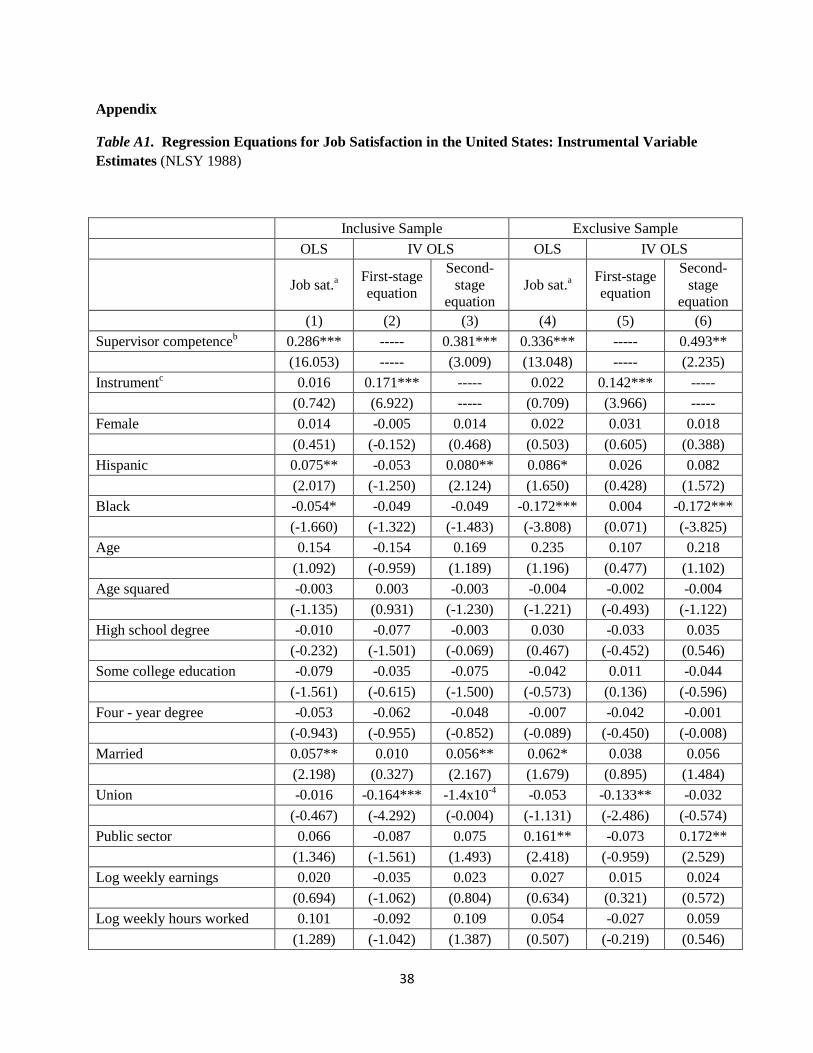
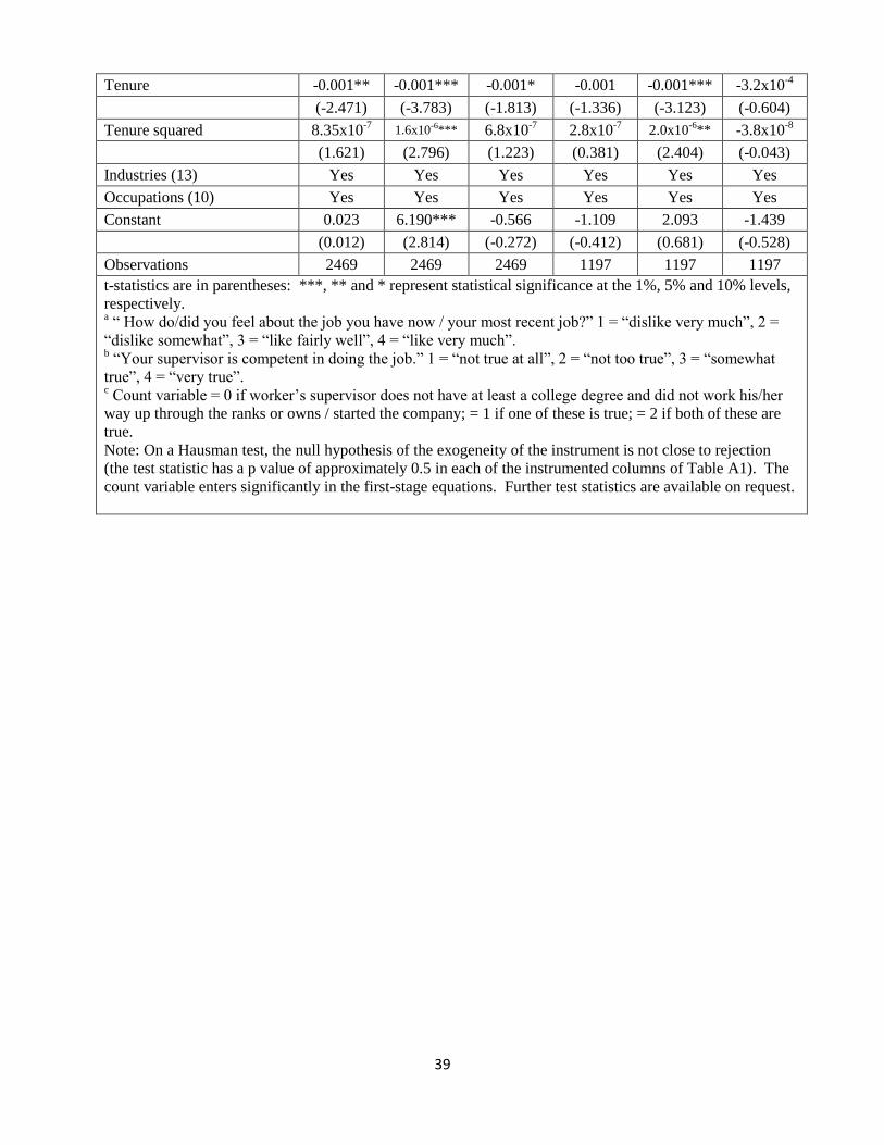
Issue 5: In principle, a valid instrument is needed for supervisor competence.

We are extremely sympathetic to, and cognizant of, such arguments; given the data available to

us it is not possible to answer this concern in a truly persuasive way. However, although we

would not wish to emphasize them, we have, in the spirit of inquiry, done some instrumental-

variable (IV) estimation. It is intrinsically difficult to obtain an instrument that satisfies the

exclusion restriction. Nevertheless, our attempted IV results are reported in Table A1 in an

15

Appendix. For this, a variable is needed that influences the competence of the supervisor and

satisfies the necessary exclusion restriction in the second-stage equation. We exploit two

possibilities. The first is whether the supervisor has a college degree; we view this as a likely

shifter in the competence equation and as a priori excludable from a worker satisfaction equation

that includes industry and occupation dummies. The second is a simple instrument. It is the

earlier variable on whether the supervisor worked his or her way up in the organization (or owns

or started the company), which could be viewed as a proxy for individual knowledge of, and

detailed experience within, the company. We might view this not as a direct variable -- as earlier

-- but instead as a candidate for inclusion in a competence equation, and one that is excludable

from the satisfaction equation as long as industry dummies are included. It is possible to

estimate such a model on the 1988 data. Columns 1 and 4 of Table A1, which are for different

sub-samples, report OLS estimates as a baseline. Column 2 is the first-stage equation, namely,

the equation for whether the supervisor is assessed as competent. The variable for the instrument

(coded 0, 1, or 2) works positively with a coefficient of 0.171 and a t-statistic of approximately

8. In column 3 of Table A1, the instrumented job-satisfaction equation has a well-determined

coefficient of 0.381 on the variable for supervisor competence. The same pattern is found in

columns 5 and 6. We would argue that these IV estimates should be treated cautiously.

Issue 6: A central role in the analysis is played by subjective assessments of the level of

supervisor competence, and these are used to define the key independent variable, so the

evidence depends on the validity of such data.

Employees seem to be in a good position to answer truthfully and fairly objectively to, for

example, an inherently factual question of the kind: “Did your supervisor work his or her way up

in this company/start the company?” To answer this in the positive does not require the worker

to like, or admire the behavior of, the supervisor. Such factual questions are routine in social-

science surveys and are widely used in almost all econometric research. In so far as people’s

answers contain measurement error (perhaps because they are new to the office or factory and

are thus not certain about the job history of their supervisor), then regression coefficients will be

biased downwards, and that will typically make it harder, not easier, to find statistically

significant results in the earlier equations.

5. Conclusion

16

Bosses are found everywhere in working life, but their activities have provoked relatively

little empirical interest among labor-market researchers. This paper offers evidence consistent

with the belief that the qualities of supervisors -- particularly their technical competence -- may

have significant and currently under-appreciated consequences for workers’ well-being. To the

best of our knowledge, these results are the first of their kind.

Seven forms of empirical support have been documented. Some are particularly simple.

These seven have different (perhaps complementary) strengths and weaknesses, but each is

consistent with the broad idea that the quality of workers’ lives is higher if the supervisor is

highly competent, in a technical sense, at his or her job6. The size of the estimates varies from

fairly substantial to strikingly large. In some equations, such as those in Table 5, the assessed

competence of the boss is the strongest predictor of employee well-being7. One weakness of our

analysis should be noted; it would be desirable to have information on an even wider range of

supervisors’ characteristics (see Artz 2013, for example, on supervisor age), and that must

largely await future data sets.

Boss competence is, admittedly, a subtle concept. There is no conventional method for

assessing it. For this reason, the paper has explored a variety of empirical proxies for technical

competence and expertise. 8

First, in a cross-section of 6000 young U.S. workers, the job

satisfaction of employees is positively correlated with whether the supervisor worked his or her

way up within the company (or literally started the company). Second, in a cross-section of 1600

British workers, satisfaction levels are higher among individuals whose supervisor could if

necessary step in competently to do that job, and where the supervisor knows his or her own job

extremely well. Third, in pooled cross-sections totaling 27,000 workers, a variable for assessed

supervisor-competence enters with a large positive coefficient in a job satisfaction equation.

Fourth, the key conclusion continues to hold -- with an only marginally reduced coefficient -- in

fixed-effects estimation. Fifth, it is also unaffected, in fixed-effects equations, by the inclusion

of an extra control variable that is a proxy for fluctuations in the underlying cheerfulness of

individuals. Sixth, it is robust, with an only fractionally reduced effect-size, in estimates that

6 As mentioned above, we have obtained the same kinds of results with other measures.

7 Figure 1 is one non-technical way to convey this.

8 Although, for simplicity, we have in some cases used a cardinalized measure of competence, Table A2 shows that

the findings are the same when the equations are re-estimated with a set of competence dummies. In further tests: (i)

Table A3 reveals that -- as a check against attrition bias -- the supervisor effect is equally strong in a sample of

workers who have recently left the employer; and (ii) there is some sign of asymmetry in the supervisor effect, in the

sense that the absolute value of the coefficient is larger when acquiring a bad supervisor rather than a good one.

17

restrict the sample solely to workers who remain in the same job in the same workplace, who are

thus the employees who experience only a change in the quality of their supervisor. Seventh,

tentative instrumental-variable estimates are reported in the Appendix.

Lazear et al. (2011) argue, in an appealing way, that bosses act to raise workers’

productivity. We agree with this. The paper has attempted, however, to consider a wider remit

for bosses. They are trainers and advisors; nevertheless, they also make organizational decisions

about how workplaces actually run. It is likely that future research will have to examine explicit

models of supervisory behavior. It will also be important to construct quasi-experimental

inquiries into the effects that stem from poor, mediocre, and talented bosses. Most especially,

true randomized trials -- where different kinds of team leaders are allocated to work teams in

some form of otherwise standardized productivity setting -- would teach us much about the size

of leaders’ effects. In the world of practice, moreover, it may be that our results could one day

be helpful to CEOs and human resources managers when making promotion decisions. Such

issues merit future attention.

18

References

Agrawal, A. & Tambe, P. 2014. Technological investment and labor outcomes: Evidence from

private equity. Working paper, Stern School, New York University.

Argyle, M. 1989. Do happy workers work harder? The effect of job satisfaction on job

performance. In: Ruut Veenhoven (ed), How harmful is happiness? Consequences of

enjoying life or not. Universitaire Pers Rotterdam, The Netherlands.

Arz, B. 2013. The impact of supervisor age on employee job satisfaction. Applied Economics

Letters 20: 1340-1343.

Artz, B. & Taengnoi, S. 2014. Do females prefer female bosses? Working paper, University of

Wisconsin - Oshkosh.

Becker, A.J. & Wrisberg, C.A. 2008. Effective coaching in action: observations of legendary

collegiate basketball coach Pat Summitt. Sport Psychologist 22: 197-211.

Benjamin, D., Heffetz, O., Kimball, M.S. & Rees-Jones, A. 2012. What do you think would

make you happier? What do you think you would choose? American Economic Review,

102(5): 2083–2110.

Bloom, N., Genakos, C., Sadun, R. & Van Reenen, J. 2012. Management practices across firms

and countries. Academy of Management Perspectives 26: 12-33.

Bockerman, P., Bryson, A. & Ilmakunnas, P. 2012. Does high-involvement management

improve worker wellbeing? Journal of Economic Behavior & Organization 84: 660-680.

Booth, A.L. & van Ours, J.C. 2008. Job satisfaction and family happiness: The part-time work

puzzle. Economic Journal 118: F77-F99.

Boxall, P. & Macky, K. 2014. High-involvement work processes, work intensification and

worker wellbeing. Work, Employment and Society 28: 963-984.

Branch, G., Hanushek, E. & Rivkin, S.G. 2013. School leaders matter: measuring the impact of

effective principals Education Next, 13, Winter.

Brandts, J. & Cooper, D. 2007. It’s not what you pay, it’s what you say: An experimental study

of the manager-employee relationship in overcoming coordination failure. Journal of

European Economic Association 5: 1223-1268.

Brown, S., Gray, D., McHardy, J. & Taylor, K. 2014. Employee trust and workplace

performance. IZA discussion paper 8284.

19

Bryson, A., Forth, J. & Kirby, S. 2005. High-involvement management practices, trade union

representation and workplace performance Scottish Journal of Political Economy 52:

451-491.

Capelli, P. & Rogovsky, N. 1998. Employee involvement and organizational citizenship:

implications for labor law reform and “lean production”, Industrial and Labor Relations

Review 51: 633-653.

Clark, A.E. 2001. What really matters in a job? Hedonic measurement using quit data. Labour

Economics 8: 223-242.

Clark, A.E. & Oswald, A.J. 1996. Satisfaction and comparison income. Journal of Public


De Neve, J. & Oswald, A.J. 2012. Estimating the influence of life satisfaction and positive affect

on later income using sibling fixed effects. Proceedings of the National Academy of

Sciences of the United States of America 109: 19953-19958.

Dezso, C. L. & Ross, D. G. 2012. Does female representation in top management improve firm

performance? A panel data investigation. Strategic Management Journal 33(9):1072-1089.

Diener, E., Suh, E.M., Lucas, R.E. & Smith, H.L. 1999. Subjective well-being: Three decades of

progress. Psychological Bulletin 125(2): 276-302.

Di Tella, R., MacCulloch, R.J. & Oswald, A.J. 2001. Preferences over inflation and

unemployment: Evidence from surveys of happiness. American Economic Review 91: 335-

341.

Easterlin, R. A. 2003. Explaining happiness. Proceedings of the National Academy of Sciences

of the United States of America 100: 11176-11183.

Edmans, A. 2012. The link between job satisfaction and firm value, with implications for

corporate social responsibility. Academy of Management Perspectives 26: 1-19.

Ehrenberg, R.G. & Smith, R.S. 2012. Modern labor economics: Theory and policy. Prentice

Hall, New York.

Filer, R.K., Hamermesh, D.S. & Rees, A. 1996. The economics of work and pay. Harper Collins,

USA.

Finkelstein, S. and Hambrick, D.C. 1996. Strategic leadership: Top executives and their effects

on organizations. West’s Strategic Management Series: Minneapolis/St.Paul, MN.

Freeman, R.B. 1978. Job satisfaction as an economic variable. American Economic Review 68:

135-141.

20

Freeman R., Kruse, D. and Blasi, J. 2008. Worker responses to shirking under shared capitalism.

National Bureau of Economic Research, NBER paper 14227.

Frey, B.S. & Stutzer, A. 2002. Happiness and economics. Princeton, USA.

Garicano, L. 2000. Hierarchies and the organization of knowledge in production. Journal of

Political Economy,108: 874-904.

Goerg, S.J., Kube, S., and Zultan, R. 2010. Treating equals unequally: Incentives in teams,

workers’ motivation, and production technology. Journal of Labor Economics 28: 747–

772.

Goodall, A.H. 2009. Socrates in the boardroom: Why research universities should be led by top

scholars, Princeton University Press, Princeton, USA.

Goodall, A.H. 2011. Physician-leaders and hospital performance: Is there an association? Social

Science & Medicine, 73 (4): 535-539.

Goodall, A.H., Kahn, L. M. & Oswald, A. J. 2011. Why do leaders matter? A study of expert

knowledge in a superstar setting. Journal of Economic Behavior & Organization 77: 265–

284.

Graham, C., Eggers, A. & Sukhtankar, S. 2004. Does happiness pay? An exploration on panel

data for Russia. Journal of Economic Behavior & Organization 55: 319-342.

Graham, C. 2011. The pursuit of happiness: An economy of well-being. Brookings Institution

Press, Washington DC.

Green, C.P. & Heywood, J.S. 2010. Profit sharing and the quality of relations with the boss.

Labour Economics 5: 859-867.

Guthrie, J.P. 2001. High-involvement work practices, turnover, and productivity: Evidence from

New Zealand. Academy of Management Journal 44: 180-190.

Halac, M. & Prat, A. 2014. Managerial attention and worker engagement. Working paper,

University of Warwick.

Hamermesh, D.S. 2001. The changing distribution of job satisfaction. Journal of Human

Resources 36: 1-30.

Helliwell, J.F. & Huang, H. 2010. How’s the job? Well-being and social capital in the

workplace. Industrial and Labor Relations Review 63: 205-227.

Heywood, J.S., Siebert, W.S., and Wei, X.D. 2002. Worker sorting and job satisfaction: The case

of union and government jobs. Industrial & Labor Relations Review 55: 595–609.

Isen, A. M. 2000. Positive affect and decision making. In M. Lewis & J. M. Haviland (Eds.),

Handbook of emotions. 2nd ed. New York: The Guilford Press.

21

Layard, R. 2006. Happiness: Lessons from a new science. Penguin Books, London.

Lazear, E.P., Shaw, K.L. & Stanton, C.T. 2011. The value of bosses. Working paper, Stanford

University.

Levy-Garboua, L., Montmarquette, C. & Simmonet, V. 2007. Job satisfaction and quits. Labour


Mackey, A. 2008. The effect of CEOs on firm performance. Strategic Management Journal 29

(12): 1357-1367.

McFarlin, D.B. & Sweeney, P.D. 1992. Distributive and procedural justice as predictors of

satisfaction with personal and organizational outcomes. Academy of Management

Journal 35: 626-637.

Miles, E.W., Patrick, S.L. & King, W.C. 1996. Job level as a systemic variable in predicting the

relationship between supervisory communication and job satisfaction. Journal of

Occupational and Organizational Psychology 69: 277-292.

Oswald, A.J. & Wu, S. 2010. Objective confirmation of subjective measures of human well-

being: Evidence from the USA. Science 327: 576-579.

Oswald, A.J., Proto, E. & Sgroi, D. 2015. Happiness and productivity. Journal of Labor

Economics, forthcoming.

Powdthavee, N. 2010. The Happiness Equation: The Surprising Economics of Our Most

Valuable Asset. Icon Books, London.

Senik, C. 2004. When information dominates comparison: Learning from Russian subjective

data. Journal of Public Economics 88: 2099-2123.

Souder, D., Simsek, Z. & Johnson, S. G. 2012. The differing effects of agent and founder CEOs

on the firm's market expansion. Strategic Management Journal 33(1): 23-41.

Thomas, A.B. 1988. Does leadership make a difference in organizational performance?

Administrative Science Quarterly 33: 388–400.

Tsai, W-C., Chen, C-C. & Liu, J-L. 2007. Test of a model linking employee positive moods and

task performance. Journal of Applied Psychology 92: 1570-1583.

Waldman, D.A. and Yammarino, F.J. 1999. CEO charismatic leadership: levels-of-management

and levels-of analysis effects. Academy of Management Review 24: 266–285.

Yukl, G. 2008. How leaders influence organizational effectiveness. Leadership Quarterly 19(6):

708-722.

23

Figure 1. An Illustration of the Major Role of Supervisor Competence (with standardized effect-sizes,

using the fixed-effects estimates of Table 5)

24

Table 1. Variable Definitions and Descriptive Statistics

Variable Definition Mean (Standard Deviation)

(1) (2) (3)

Job satisfaction

(NLSY data)

Global job satisfaction: = 1 if “dislike very

much” to 4 if “like very much” .

3.181

(0.749)

3.295

(0.728) -----

Job satisfaction

(WIB data)

Global job satisfaction: = 1 if “completely

dissatisfied” to 7 if “completely satisfied”. ----- -----

5.305

(1.101)

Supervisor

competence

Supervisor is competent in doing the job: = 1 if

“not true at all” to 4 if “very true”.

3.489

(0.748) ----- -----

Supervisor

expertise

= 1 if supervisor “worked way up through ranks”

or “started or owns company” or 0 otherwise. -----

0.683

(0.465) -----

Supervisor

knowledge

Supervisor “knows their own job well”: = 1 if

“not at all true” to 4 if “very true”. ----- -----

3.236

(0.904)

Supervisor

replacement

Supervisor “could do [worker’s] job if [worker]

was away”: =1 “not true at all” to 4 if “very

true”.

----- ----- 2.523

(1.216)

Friendly Your co-workers are friendly: = 1 if “not true at

all” to 4 if “very true”.

3.630

(0.588) ----- -----

Best You are given a chance to do the things you do

best: = 1 if “not true at all” to 4 if “very true”.

3.085

(0.887) ----- -----

Female = 1 if worker is female and 0 if male. 0.466

(0.499)

0.444

(0.497)

0.529

(0.499)

Hispanic = 1 if worker is Hispanic and 0 otherwise. 0.161

(0.368)

0.156

(0.363) -----

Black = 1 if worker is Black and 0 otherwise. 0.217

(0.413)

0.245

(0.431) -----

High school = 1 if worker has only a high school degree and 0

otherwise.

0.445

(0.497)

0.429

(0.495) -----

Some college = 1 if worker has more than a high school degree

but not a 4-year degree and 0 otherwise.

0.196

(0.397)

0.223

(0.416) -----

College = 1 if worker has at least a 4-year degree and 0

otherwise.

0.090

(0.286)

0.208

(0.406) -----

Degree or higher = 1 if worker has a degree, equivalent or higher

and 0 otherwise. ----- -----

0.302

(0.459)

A / AS level = 1 if worker has A-level or AS-level education

and 0 otherwise. ----- -----

0.112

(0.316)

O level = 1 if worker has O-level education and 0

otherwise. ----- -----

0.252

(0.435)

CSE = 1 if worker has CSE education and 0

otherwise. ----- -----

0.111

(0.314)

Married = 1 if worker is married and 0 otherwise. 0.283

(0.451)

0.523

(0.500)

0.653

(0.476)

Union = 1 if worker is a member of a labor union and 0

otherwise.

0.174

(0.379)

0.138

(0.345)

0.327

(0.469)

Public = 1 if worker’s employer is a government

institution and 0 otherwise.

0.111

(0.315)

0.131

(0.338)

0.300

(0.458)

Age Age in years 22.160

(3.842)

29.038

(2.254)

38.501

(10.584)

Age squared Age in years x age in years 505.81 848.31 1594.29

25

(178.14) (131.60) (840.39)

Tenure Tenure at employer in weeks 78.21

(96.31)

177.15

(172.64)

386.71

(389.09)

Tenure squared Tenure at employer x tenure at employer 15391

(41683)

61182

(101907)

300842

(567750)

Log hours Natural log of weekly hours worked 3.555

(0.400)

3.731

(0.150)

3.454

(0.427)

Log earnings Natural log of weekly earnings at job 5.141

(0.763)

5.918

(0.622)

5.553

(0.775)

Column (1): Observations = 27,537 across five NLSY waves (1979, 1980, 1981, 1982, 1988). 10

occupation categories and 13 industry categories are included.

Column (2): Observations = 6,298 in NLSY 1990 wave. 10 occupation categories, 13 industry

categories, and 4 firm size categories are included.

Column (3): Observations = 1,604 in Working in Britain 2000. 9 occupation categories, 9 industry

categories and 3 firm size categories are included.

26

Table 2. Regression Equations for Job Satisfaction in the United States: OLS Cross-Section

Estimates (NLSY 1990 data)

Job satisfactiona

(1) (2)

Supervisor “worked way up in the ranks” or 0.047** -----

“started or owns company”b (2.009) -----

Supervisor “worked way up in the ranks” ----- 0.044*

----- (1.782)

Supervisor “started or owns company” ----- 0.059

----- (1.612)

Female 0.031 0.030

(1.143) (1.120)

Hispanic 0.075*** 0.075***

(2.663) (2.668)

Black -0.062** -0.062**

(-2.413) (-2.382)

Age 0.064 0.064

(0.479) (0.478)

Age squared -0.001 -0.001

(-0.473) (-0.473)

High school degree -0.031 -0.031

(-0.836) (-0.837)

Some college education -0.046 -0.046

(-1.105) (-1.099)

Four-year college degree -0.084* -0.083*

(-1.789) (-1.780)

Married 0.062*** 0.062***

(2.761) (2.778)

Union -0.049 -0.048

(-1.498) (-1.453)

Public sector 0.136*** 0.137***

(3.279) (3.300)

Log weekly earnings 0.115*** 0.115***

(4.568) (4.550)

Log weekly hours worked 0.230*** 0.230***

(2.893) (2.892)

Tenure -4.9x10-4

** -4.9x10-4

**

(-2.417) (-2.412)

Tenure squared 2.80x10-7

2.79x10-7

(0.846) (0.844)

Firm sizes (4) Yes Yes

Industries (13) Yes Yes

Occupations (10) Yes Yes

Constant 0.973 0.972

(0.498) (0.497)

Observations 6298 6298

t-statistics are in parentheses: ***, ** and * represent statistical significance at the 1%, 5% and

10% levels, respectively. Survey weights are used throughout.

27

a “ How do/did you feel about the job you have now / your most recent job?” 1 = “dislike very

much”, 2 = “dislike somewhat”, 3 = “like fairly well”, 4 = “like very much”. b “To the best of your knowledge, what reason on this card best explains how he/she came to

occupy his/her position?” 1 = “worked way up through ranks” or “started or owns company” and

0 = otherwise.

28

Table 3. Regression Equations for Job Satisfaction in Great Britain: OLS Cross-Section Estimates

(WIB 2000 data)

Job satisfactiona

(1) (2) (3)

Supervisor “could do [worker’s] job”b 0.132*** ----- 0.055**

(5.321) ----- (2.086)

Supervisor “knows own job”c ----- 0.305*** 0.279***

----- (8.633) (7.371)

Female 0.227*** 0.212*** 0.213***

(3.193) (3.065) (3.074)

Age -0.033 -0.047** -0.044**

(-1.526) (-2.237) (-2.125)

Age squared 4.47x10-4

* 0.001** 0.001**

(1.657) (2.382) (2.284)

Degree or higher -0.142 -0.182* -0.178*

(-1.349) (-1.762) (-1.727)

A-level or AS-level -0.175 -0.210* -0.206*

(-1.506) (-1.836) (-1.802)

O-level -0.212** -0.222** -0.223**

(-2.243) (-2.368) (-2.385)

CSE -0.052 -0.058 -0.065

(-0.489) (-0.552) (-0.622)

Married 0.106 0.123* 0.118*

(1.621) (1.943) (1.847)

Union -0.183** -0.146** -0.147**

(-2.484) (-2.040) (-2.058)

Public sector 0.117 0.149* 0.146*

(1.413) (1.842) (1.815)

Log weekly hours worked -0.237*** -0.207** -0.204**

(-2.693) (-2.414) (-2.383)

Log annual salary 0.211*** 0.192*** 0.201***

(3.456) (3.124) (3.304)

Tenure 1.84x10-4

1.92x10-4

2.30x10-4

(0.816) (0.834) (1.003)

Tenure squared -1.41x10-7

-1.38x10-7

-1.59x10-7

(-0.863) (-0.796) (-0.924)

Firm sizes (3) Yes Yes Yes

Industries (9) Yes Yes Yes

Occupations (9) Yes Yes Yes

Constant 5.239*** 4.814*** 4.634***

29

(9.746) (9.197) (8.867)

Observations 1604 1604 1604

t-statistics are in parentheses: ***, ** and * represent statistical significance at the 1%,

5% and 10% levels, respectively. Survey weights are used throughout.

a “All in all, how satisfied would you say you are with your job?” Range from 1 =

“completely dissatisfied” to 7 = “completely satisfied”.

b “How true is it that your supervisor could do your job if you were away?” 1 = “not at

all true”, 2 = “somewhat true”, 3 = “true”, 4 = “very true”.

c “How true is it that your supervisor or manager knows their own job well?” 1 = “not

at all true”, 2 = “somewhat true”, 3 = “true”, 4 = “very true”.

30

Table 4. Regression Equations for Job Satisfaction in the United States: Pooled Cross-Section

Estimates (NLSY 1979-1982, 1988)

Job satisfactiona

(1) (2) (3) (4) (5)

Supervisor competenceb 0.303*** 0.303*** 0.301*** 0.293*** 0.238***

(35.187) (35.155) (34.890) (34.057) (26.616)

Co-workers are friendlyc ----- ----- ----- ----- 0.225***

----- ----- ----- ----- (20.243)

Female 0.039*** 0.037*** 0.065*** 0.057*** 0.062***

(3.026) (2.814) (4.896) (3.837) (4.274)

Hispanic 0.004 0.003 -0.004 0.002 0.010

(0.277) (0.200) (-0.243) (0.129) (0.710)

Black -0.110*** -0.102*** -0.097*** -0.081*** -0.054***

(-7.600) (-6.993) (-6.551) (-5.472) (-3.704)

Age 0.033** 0.034** -0.031* -0.024 -0.023

(2.274) (2.121) (-1.739) (-1.360) (-1.330)

Age squared -3.83x10-4

-4.59x10-4

0.001* 0.001 4.89x10-4

(-1.232) (-1.353) (1.885) (1.378) (1.334)

High school degree ----- -0.017 -0.039** -0.060*** -0.055***

----- (-1.074) (-2.384) (-3.641) (-3.456)

Some college education ----- -0.014 -0.026 -0.084*** -0.081***

----- (-0.690) (-1.265) (-3.894) (-3.861)

Four - year degree ----- 0.009 -0.057** -0.196*** -0.201***

----- (0.361) (-2.214) (-7.017) (-7.332)

Married ----- 0.049*** 0.042*** 0.043*** 0.044***

----- (3.488) (2.993) (3.094) (3.170)

Union ----- ----- -0.066*** -0.039** -0.031**

----- ----- (-4.001) (-2.370) (-1.964)

Public sector ----- ----- 0.137*** 0.051** 0.052**

----- ----- (6.877) (2.024) (2.116)

Log weekly earnings ----- ----- 0.110*** 0.093*** 0.092***

----- ----- (8.065) (6.719) (6.834)

Log weekly hours worked ----- ----- 0.038* 0.052** 0.051**

----- ----- (1.862) (2.502) (2.472)

Tenure ----- ----- -9.10x10-5

-1.76x10-4

-1.74x10-4

----- ----- (-0.655) (-1.265) (-1.269)

Tenure squared ----- ----- 4.19x10-9

1.41x10-7

1.52x10-7

----- ----- (0.015) (0.501) (0.547)

Industries (13) No No No Yes Yes

Occupations (10) No No No Yes Yes

Year dummies No No No Yes Yes

31

Constant 1.592*** 1.598*** 1.771*** 2.086*** 1.441***

(9.385) (8.528) (9.295) (10.415) (7.214)

Observations 27537 27537 27537 27537 27537

t-statistics are in parentheses: ***, ** and * represent statistical significance at the 1%, 5% and 10%

levels, respectively. Survey weights are used throughout. Standard errors are clustered by individual

respondent. a “ How do/did you feel about the job you have now / your most recent job?” 1 = “dislike very much”, 2 =

“dislike somewhat”, 3 = “like fairly well”, 4 = “like very much”. b “Your supervisor is competent in doing the job.” 1 = “not true at all”, 2 = “not too true”, 3 = “somewhat

true”, 4 = “very true”. c “Your co-workers are friendly.” 1 = “not true at all”, 2 = “not too true”, 3 = “somewhat true”, 4 = “very

true”.

32

Table 5. Regression Equations for Job Satisfaction in the United States: Fixed-Effects Estimates

(NLSY 1979-1982, 1988)

Job satisfactiona

(1) (2) (3) (4) (5)

Supervisor competenceb 0.243*** 0.243*** 0.239*** 0.233*** 0.198***

(28.790) (28.767) (28.183) (27.647) (22.951)

Co-workers are friendlyc ----- ----- ----- ----- 0.165***

----- ----- ----- ----- (14.993)

Age 0.039*** 0.040** -0.001 -0.028 -0.025

(2.789) (2.374) (-0.064) (-1.192) (-1.078)

Age squared -4.75x10-4

* -0.001 2.55x10-4

4.37x10-4

3.74x10-4

(-1.618) (-1.530) (0.696) (1.169) (1.007)

High school degree ----- -0.017 -0.065*** -0.074*** -0.066***

----- (-0.745) (-2.800) (-3.235) (-2.911)

Some college education ----- -0.011 -0.079** -0.114*** -0.105***

----- (-0.339) (-2.473) (-3.594) (-3.342)

Four - year degree ----- 0.035 -0.142*** -0.242*** -0.239***

----- (0.892) (-3.398) (-5.699) (-5.688)

Married ----- 0.014 0.018 0.015 0.016

----- (0.883) (1.147) (0.975) (1.059)

Union ----- ----- -0.004 0.007 0.011

----- ----- (-0.264) (0.459) (0.742)

Public sector ----- ----- 0.149*** 0.059** 0.061**

----- ----- (7.115) (2.367) (2.471)

Log weekly earnings ----- ----- 0.123*** 0.118*** 0.117***

----- ----- (7.709) (7.325) (7.366)

Log weekly hours worked ----- ----- -0.004 -0.003 -0.004

----- ----- (-0.194) (-0.148) (-0.190)

Tenure ----- ----- -0.001*** -0.001*** -0.001***

----- ----- (-4.879) (-5.439) (-5.243)

Tenure squared ----- ----- 4.60x10-7

* 6.13x10-7

** 5.93x10-7

**

(1.715) (2.276) (2.212)

Industries (13) No No No Yes Yes

Occupations (10) No No No Yes Yes

Year dummies No No No Yes Yes

Constant 1.718*** 1.710*** 1.708*** 2.361*** 1.853***

(10.514) (8.772) (8.600) (6.684) (5.261)

Observations 27537 27537 27537 27537 27537


levels, respectively. Standard errors are clustered by individual respondent.

33

a “ How do/did you feel about the job you have now / your most recent job?” 1 = “dislike very much”, 2 =



true”.

34

Table 6. Regression Equations for Job Satisfaction in the United States: Alternative Groupings

Fixed-Effects Estimates (NLSY 1979-1982)

(This table gradually restricts the sample to show, in the final column, that the FE results hold even when

the sample is only those workers who remain within the same job and workplace, namely, when only

supervision alters.)

Job satisfactiona

Narrow sample 1 Narrower sample 2 Narrowest sample 3

Supervisor competenceb 0.179*** 0.149*** 0.121***

(16.420) (10.375) (4.926)

Co-workers are friendlyc 0.160*** 0.100*** 0.064**

(11.800) (5.965) (2.485)

Age -0.138** -0.129 -0.046

(-1.979) (-1.294) (-0.223)

Age squared 0.004** 0.004* 0.001

(2.534) (1.653) (0.185)

High school degree -0.084*** -0.057 -0.051

(-2.890) (-1.364) (-0.749)

Some college education -0.162*** -0.118* -0.102

(-3.618) (-1.755) (-0.939)

Four - year degree -0.446*** -0.432*** -0.839***

(-6.040) (-3.396) (-4.288)

Married 0.002 -0.037 0.022

(0.102) (-1.185) (0.382)

Union -0.003 0.019 0.004

(-0.144) (0.722) (0.095)

Public sector 0.093*** 0.158*** 0.171*

(2.712) (2.754) (1.930)

Log weekly earnings 0.126*** 0.042 0.048

(5.564) (1.490) (1.011)

Log weekly hours worked 0.006 0.029 0.000

(0.191) (0.586) (0.005)

Tenure -0.002*** -0.004*** -0.006***

(-5.062) (-8.198) (-4.238)


6.47x10-6

*** 9.65x10-6

***

(0.502) (4.085) (3.359)

Industries (13) Yes Yes No

Occupations (10) Yes Yes No

Year dummies Yes Yes Yes

Constant 2.828*** 3.484*** 3.180

(3.499) (3.104) (1.437)

Observations 19587 9361 3275

35


levels, respectively. Standard errors are clustered by each cluster type in the corresponding columns. a “ How do/did you feel about the job you have now / your most recent job?” 1 = “dislike very much”, 2 =



true”.

Sample 1: all observations from 1979 – 1982 are included.

Sample 2: only observations of workers in the same employer are included.

Sample 3: only observations of workers in same employer, occupation and industry are included.

Note

The number of third-column observations is reduced (i.e. groupings large) because we use 3-digit

occupations and industries to generate the sample/groupings. This corresponds to very close job-matches

across the waves.

36

Table 7. Regression Equations for Job Satisfaction and Am-Given-Chance-To-Do-My-Best in the

United States: Robustness Checks

Job satisfactiona – Fixed effects Can do what does best

d

Whole

sample

NLSY 1979, 1980, 1988 Pooled

cross-sect.

Fixed

effects Small firme

Big firme

(1) (2) (3) (4) (5)

Supervisor competenceb 0.110** 0.194*** 0.125*** 0.207*** 0.183***

(2.299) (7.784) (4.557) (20.818) (19.291)

Co-workers are friendlyc 0.165*** 0.150*** 0.162*** 0.160*** 0.135***

(15.011) (4.868) (4.830) (13.315) (11.215)

Female ----- ----- ----- 0.123 -----

----- ----- ----- (-7.030) -----

Hispanic ----- ----- ----- 0.043 -----

----- ----- ----- (-2.347) -----

Black ----- ----- ----- -0.006 -----

----- ----- ----- (-0.352) -----

Age x supervisor comp. 0.004* ----- ----- ----- -----

(1.846) ----- ----- ----- -----

Age -0.040 -0.007 0.042 0.076*** 0.015

(-1.604) (-0.131) (0.555) (3.702) (0.554)

Age squared 3.91x10-4

0.001 -0.001 -0.001*** -0.001

(1.055) (0.606) (-0.446) (-3.185) (-1.258)

High school degree -0.067*** 0.019 -0.181** -0.081*** -0.051*

(-2.941) (0.317) (-2.478) (-4.019) (-1.868)

Some college education -0.106*** 0.045 -0.190* -0.179*** -0.073*

(-3.372) (0.521) (-1.878) (-6.890) (-1.934)

Four - year degree -0.242*** -0.065 -0.345** -0.224*** 0.032

(-5.742) (-0.594) (-2.478) (-7.077) (0.637)

Married 0.016 -0.011 -0.018 0.021 0.019

(1.053) (-0.270) (-0.369) (1.365) (1.097)

Union 0.012 0.035 -0.077 -0.096*** -0.027

(0.796) (0.713) (-1.577) (-4.943) (-1.474)

Public sector 0.062** 0.207** 0.354*** -0.016 -0.036

(2.508) (2.152) (2.634) (-0.535) (-1.181)

Log weekly earnings 0.117*** 0.042 0.061 0.105*** 0.116***

(7.346) (0.979) (1.370) (7.087) (6.661)

Log weekly hours worked -0.004 0.113** 0.073 0.160*** 0.071***

(-0.162) (2.093) (0.978) (6.557) (2.756)

Tenure -0.001*** -0.001 -0.001 0.001*** 0.001***

(-5.192) (-1.397) (-1.505) (6.912) (3.209)

37


** 4.50x10-7

8.09x10-7

-1.76x10-6

*** -1.21x10-6

***

(2.205) (0.698) (0.968) (-5.364) (-3.925)

Industries (13) Yes Yes Yes Yes Yes

Occupations (10) Yes Yes Yes Yes Yes

Year dummies Yes Yes Yes Yes Yes

Constant 2.163*** 1.431* 1.504 -0.072 1.177***

(5.520) (1.740) (1.286) (-0.301) (2.943)

Observations 27537 8009 6339 27537 27537


levels, respectively. Survey weights are used throughout. Standard errors are clustered by individual

respondent. a “ How do/did you feel about the job you have now / your most recent job?” 1 = “dislike very much”, 2 =



true”. d “You are given the chance to do the things you do best.” 1 = “not at all true”, 2 = “not too true”, 3 =

“somewhat true”, 4 = “very true”. e Big firms have more than 49 employees and small firms have less than 50 employees.

38

Appendix

Table A1. Regression Equations for Job Satisfaction in the United States: Instrumental Variable

Estimates (NLSY 1988)

Inclusive Sample Exclusive Sample

OLS IV OLS OLS IV OLS

Job sat.a

First-stage

equation

Second-

stage

equation

Job sat.a

First-stage

equation

Second-

stage

equation

(1) (2) (3) (4) (5) (6)

Supervisor competenceb 0.286*** ----- 0.381*** 0.336*** ----- 0.493**

(16.053) ----- (3.009) (13.048) ----- (2.235)

Instrumentc 0.016 0.171*** ----- 0.022 0.142*** -----

(0.742) (6.922) ----- (0.709) (3.966) -----

Female 0.014 -0.005 0.014 0.022 0.031 0.018

(0.451) (-0.152) (0.468) (0.503) (0.605) (0.388)

Hispanic 0.075** -0.053 0.080** 0.086* 0.026 0.082

(2.017) (-1.250) (2.124) (1.650) (0.428) (1.572)

Black -0.054* -0.049 -0.049 -0.172*** 0.004 -0.172***

(-1.660) (-1.322) (-1.483) (-3.808) (0.071) (-3.825)

Age 0.154 -0.154 0.169 0.235 0.107 0.218

(1.092) (-0.959) (1.189) (1.196) (0.477) (1.102)

Age squared -0.003 0.003 -0.003 -0.004 -0.002 -0.004

(-1.135) (0.931) (-1.230) (-1.221) (-0.493) (-1.122)

High school degree -0.010 -0.077 -0.003 0.030 -0.033 0.035

(-0.232) (-1.501) (-0.069) (0.467) (-0.452) (0.546)

Some college education -0.079 -0.035 -0.075 -0.042 0.011 -0.044

(-1.561) (-0.615) (-1.500) (-0.573) (0.136) (-0.596)

Four - year degree -0.053 -0.062 -0.048 -0.007 -0.042 -0.001

(-0.943) (-0.955) (-0.852) (-0.089) (-0.450) (-0.008)

Married 0.057** 0.010 0.056** 0.062* 0.038 0.056

(2.198) (0.327) (2.167) (1.679) (0.895) (1.484)

Union -0.016 -0.164*** -1.4x10-4

-0.053 -0.133** -0.032

(-0.467) (-4.292) (-0.004) (-1.131) (-2.486) (-0.574)

Public sector 0.066 -0.087 0.075 0.161** -0.073 0.172**

(1.346) (-1.561) (1.493) (2.418) (-0.959) (2.529)

Log weekly earnings 0.020 -0.035 0.023 0.027 0.015 0.024

(0.694) (-1.062) (0.804) (0.634) (0.321) (0.572)

Log weekly hours worked 0.101 -0.092 0.109 0.054 -0.027 0.059

(1.289) (-1.042) (1.387) (0.507) (-0.219) (0.546)

39

Tenure -0.001** -0.001*** -0.001* -0.001 -0.001*** -3.2x10-4

(-2.471) (-3.783) (-1.813) (-1.336) (-3.123) (-0.604)


1.6x10-6*** 6.8x10-7

2.8x10-7

2.0x10-6

** -3.8x10-8

(1.621) (2.796) (1.223) (0.381) (2.404) (-0.043)

Industries (13) Yes Yes Yes Yes Yes Yes

Occupations (10) Yes Yes Yes Yes Yes Yes

Constant 0.023 6.190*** -0.566 -1.109 2.093 -1.439

(0.012) (2.814) (-0.272) (-0.412) (0.681) (-0.528)

Observations 2469 2469 2469 1197 1197 1197

t-statistics are in parentheses: ***, ** and * represent statistical significance at the 1%, 5% and 10% levels,

respectively. a “ How do/did you feel about the job you have now / your most recent job?” 1 = “dislike very much”, 2 =


true”, 4 = “very true”. c Count variable = 0 if worker’s supervisor does not have at least a college degree and did not work his/her

way up through the ranks or owns / started the company; = 1 if one of these is true; = 2 if both of these are

true.

Note: On a Hausman test, the null hypothesis of the exogeneity of the instrument is not close to rejection

(the test statistic has a p value of approximately 0.5 in each of the instrumented columns of Table A1). The

count variable enters significantly in the first-stage equations. Further test statistics are available on request.

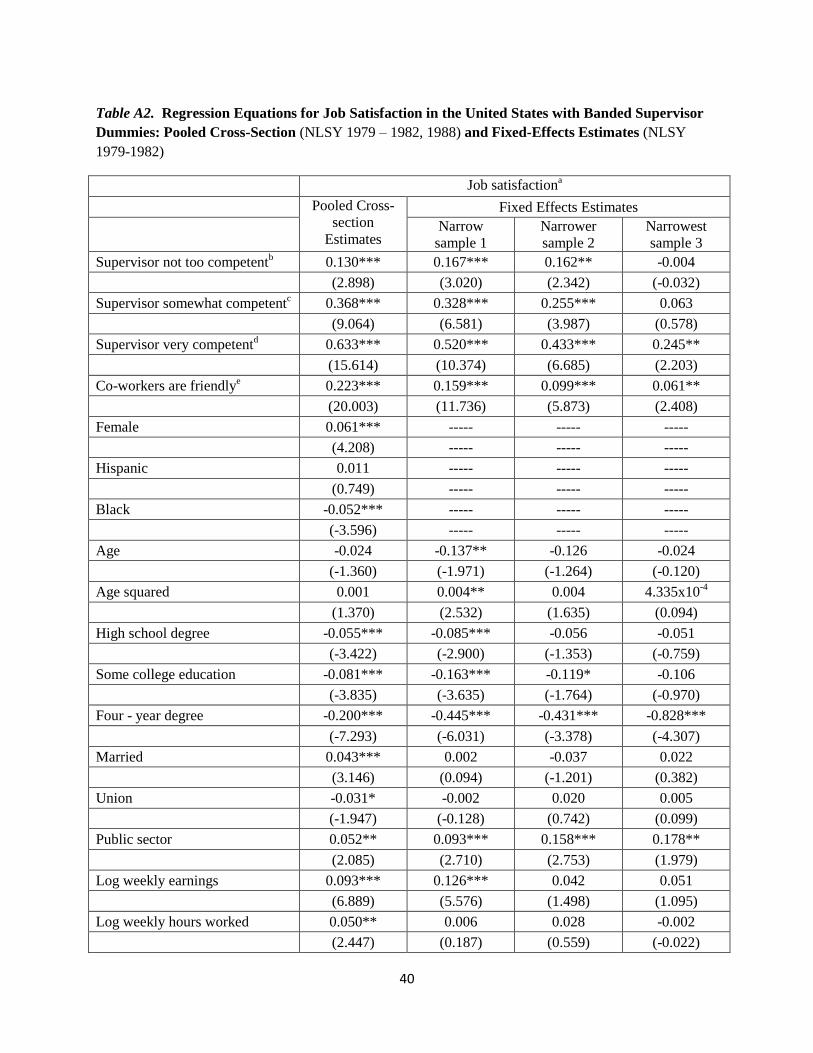
40

Table A2. Regression Equations for Job Satisfaction in the United States with Banded Supervisor

Dummies: Pooled Cross-Section (NLSY 1979 – 1982, 1988) and Fixed-Effects Estimates (NLSY

1979-1982)

Job satisfaction

a

Pooled Cross-

section

Estimates

Fixed Effects Estimates

Narrow

sample 1

Narrower

sample 2

Narrowest

sample 3

Supervisor not too competentb 0.130*** 0.167*** 0.162** -0.004

(2.898) (3.020) (2.342) (-0.032)

Supervisor somewhat competentc 0.368*** 0.328*** 0.255*** 0.063

(9.064) (6.581) (3.987) (0.578)

Supervisor very competentd 0.633*** 0.520*** 0.433*** 0.245**

(15.614) (10.374) (6.685) (2.203)

Co-workers are friendlye 0.223*** 0.159*** 0.099*** 0.061**

(20.003) (11.736) (5.873) (2.408)

Female 0.061*** ----- ----- -----

(4.208) ----- ----- -----

Hispanic 0.011 ----- ----- -----

(0.749) ----- ----- -----

Black -0.052*** ----- ----- -----

(-3.596) ----- ----- -----

Age -0.024 -0.137** -0.126 -0.024

(-1.360) (-1.971) (-1.264) (-0.120)

Age squared 0.001 0.004** 0.004 4.335x10-4

(1.370) (2.532) (1.635) (0.094)

High school degree -0.055*** -0.085*** -0.056 -0.051

(-3.422) (-2.900) (-1.353) (-0.759)

Some college education -0.081*** -0.163*** -0.119* -0.106

(-3.835) (-3.635) (-1.764) (-0.970)

Four - year degree -0.200*** -0.445*** -0.431*** -0.828***

(-7.293) (-6.031) (-3.378) (-4.307)

Married 0.043*** 0.002 -0.037 0.022

(3.146) (0.094) (-1.201) (0.382)

Union -0.031* -0.002 0.020 0.005

(-1.947) (-0.128) (0.742) (0.099)

Public sector 0.052** 0.093*** 0.158*** 0.178**

(2.085) (2.710) (2.753) (1.979)

Log weekly earnings 0.093*** 0.126*** 0.042 0.051

(6.889) (5.576) (1.498) (1.095)

Log weekly hours worked 0.050** 0.006 0.028 -0.002

(2.447) (0.187) (0.559) (-0.022)

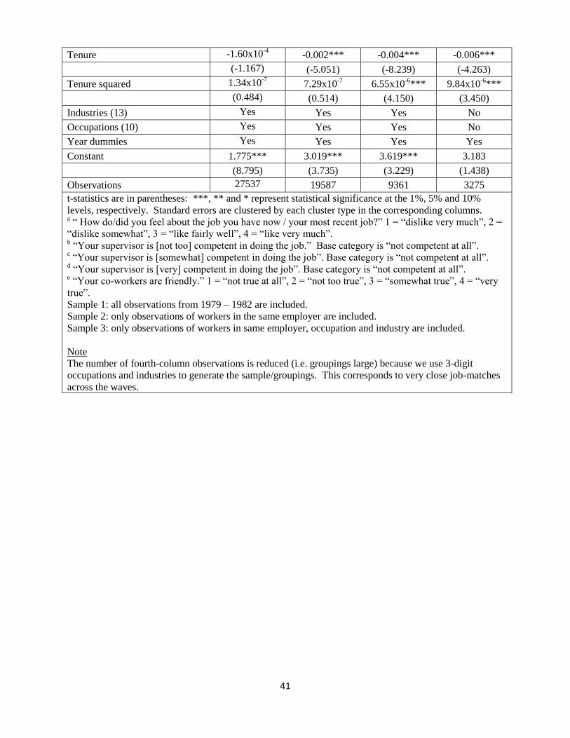
41

Tenure -1.60x10-4

-0.002*** -0.004*** -0.006***

(-1.167) (-5.051) (-8.239) (-4.263)


7.29x10-7

6.55x10-6

*** 9.84x10-6

***

(0.484) (0.514) (4.150) (3.450)

Industries (13) Yes Yes Yes No

Occupations (10) Yes Yes Yes No

Year dummies Yes Yes Yes Yes

Constant 1.775*** 3.019*** 3.619*** 3.183

(8.795) (3.735) (3.229) (1.438)

Observations 27537 19587 9361 3275



“dislike somewhat”, 3 = “like fairly well”, 4 = “like very much”. b “Your supervisor is [not too] competent in doing the job.” Base category is “not competent at all”.

c “Your supervisor is [somewhat] competent in doing the job”. Base category is “not competent at all”.

d “Your supervisor is [very] competent in doing the job”. Base category is “not competent at all”.

e “Your co-workers are friendly.” 1 = “not true at all”, 2 = “not too true”, 3 = “somewhat true”, 4 = “very

true”.

Sample 1: all observations from 1979 – 1982 are included.

Sample 2: only observations of workers in the same employer are included.

Sample 3: only observations of workers in same employer, occupation and industry are included.

Note

The number of fourth-column observations is reduced (i.e. groupings large) because we use 3-digit


across the waves.

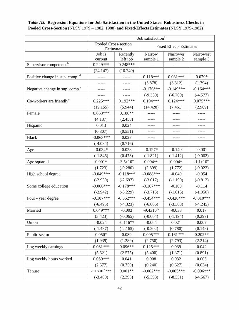
42

Table A3. Regression Equations for Job Satisfaction in the United States: Robustness Checks in

Pooled Cross-Section (NLSY 1979 – 1982, 1988) and Fixed-Effects Estimates (NLSY 1979-1982)

Job satisfaction

a

Pooled Cross-section

Estimates Fixed Effects Estimates

Job is

current

Recently

left job

Narrow

sample 1

Narrower

sample 2

Narrowest

sample 3

Supervisor competenceb 0.229*** 0.248*** ----- ----- -----

(24.147) (10.749) ----- ----- -----

Positive change in sup. comp. d ----- ----- 0.118*** 0.081*** 0.079*

----- ----- (5.878) (3.312) (1.794)

Negative change in sup. comp.e ----- ----- -0.176*** -0.149*** -0.164***

----- ----- (-9.330) (-6.700) (-4.577)

Co-workers are friendlyc 0.225*** 0.192*** 0.194*** 0.124*** 0.075***

(19.155) (5.944) (14.428) (7.461) (2.989)

Female 0.063*** 0.100** ----- ----- -----

(4.137) (2.458) ----- ----- -----

Hispanic 0.013 0.024 ----- ----- -----

(0.807) (0.551) ----- ----- -----

Black -0.063*** 0.027 ----- ----- -----

(-4.084) (0.716) ----- ----- -----

Age -0.034* 0.028 -0.127* -0.140 -0.001

(-1.846) (0.478) (-1.821) (-1.412) (-0.002)

Age squared 0.001* -3.5x10-4

0.004** 0.004* -1.1x10-4

(1.723) (-0.280) (2.399) (1.772) (-0.023)

High school degree -0.049*** -0.118*** -0.088*** -0.049 -0.054

(-2.930) (-2.697) (-3.017) (-1.190) (-0.812)

Some college education -0.066*** -0.178*** -0.167*** -0.109 -0.114

(-2.942) (-3.229) (-3.715) (-1.615) (-1.050)

Four - year degree -0.187*** -0.362*** -0.454*** -0.428*** -0.810***

(-6.495) (-4.323) (-6.006) (-3.308) (-4.245)

Married 0.049*** -0.003 -9.4x10-5

-0.038 0.017

(3.423) (-0.065) (-0.004) (-1.194) (0.297)

Union -0.024 -0.116** -0.004 0.021 0.007

(-1.437) (-2.165) (-0.202) (0.780) (0.148)

Public sector 0.050* 0.089 0.095*** 0.161*** 0.202**

(1.939) (1.289) (2.750) (2.793) (2.214)

Log weekly earnings 0.081*** 0.096** 0.125*** 0.039 0.042

(5.621) (2.575) (5.400) (1.371) (0.891)

Log weekly hours worked 0.059*** 0.041 0.008 0.032 0.003

(2.677) (0.750) (0.240) (0.627) (0.034)

Tenure -5.0x10-4

*** 0.001** -0.002*** -0.005*** -0.006***

(-3.480) (2.393) (-5.398) (-8.331) (-4.567)

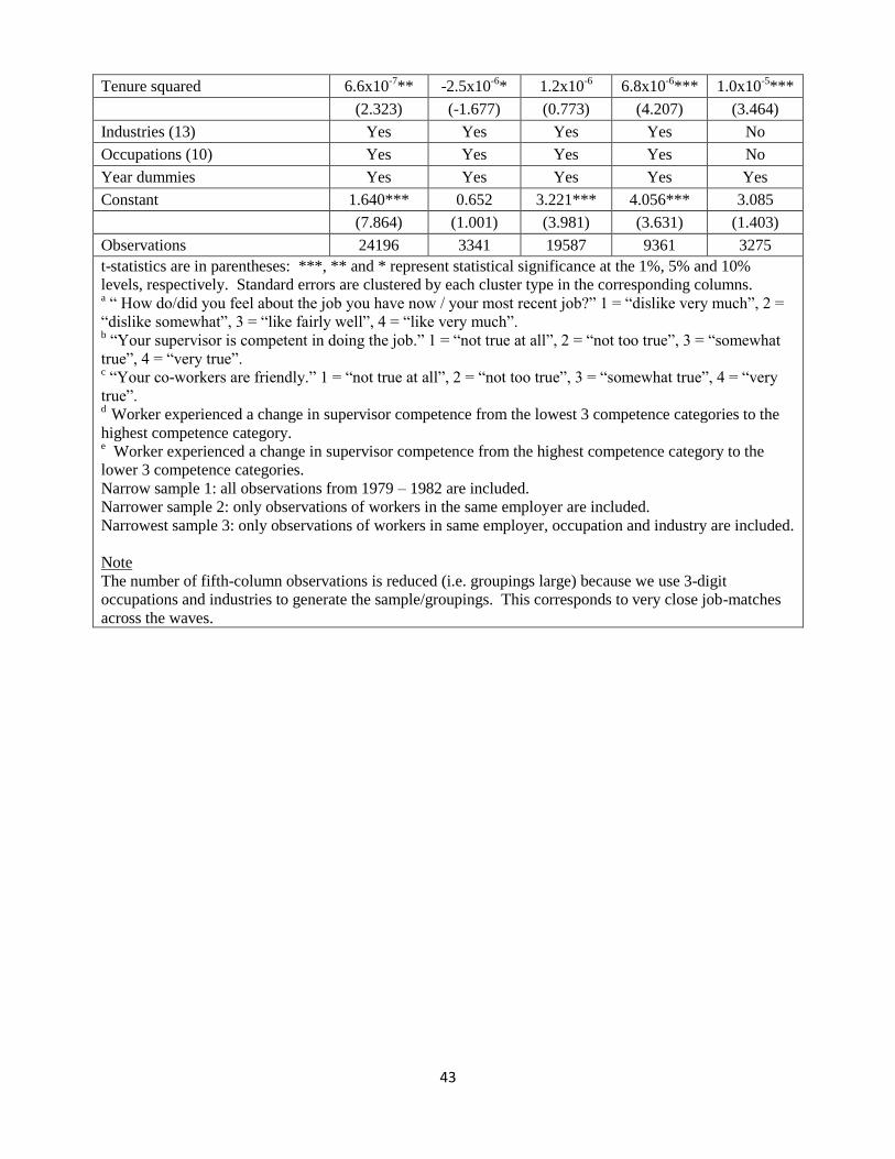
43


** -2.5x10-6

* 1.2x10-6

6.8x10-6

*** 1.0x10-5

***

(2.323) (-1.677) (0.773) (4.207) (3.464)

Industries (13) Yes Yes Yes Yes No

Occupations (10) Yes Yes Yes Yes No

Year dummies Yes Yes Yes Yes Yes

Constant 1.640*** 0.652 3.221*** 4.056*** 3.085

(7.864) (1.001) (3.981) (3.631) (1.403)

Observations 24196 3341 19587 9361 3275





true”. d

Worker experienced a change in supervisor competence from the lowest 3 competence categories to the

highest competence category. e Worker experienced a change in supervisor competence from the highest competence category to the

lower 3 competence categories.

Narrow sample 1: all observations from 1979 – 1982 are included.

Narrower sample 2: only observations of workers in the same employer are included.

Narrowest sample 3: only observations of workers in same employer, occupation and industry are included.

Note

The number of fifth-column observations is reduced (i.e. groupings large) because we use 3-digit


across the waves.

boss competence and worker well-being€¦ · boss competence and worker well-being ... economics...

Documents