boston college and diw berlin - · pdf fileboston college and diw berlin ... the estimates...
TRANSCRIPT

Automation and Programming with Stata
Christopher F Baum
Boston College and DIW Berlin
NCER, Queensland University of Technology, March 2014
Christopher F Baum (BC / DIW) Automation & Programming NCER/QUT, 2014 1 / 179

Overview
Overview
This talk focuses on several ways in which you can use Stata as aprogramming language to automate your data management andstatistics tasks and perform them more efficiently. We first discussStata’s capabilities, augmented by several user-written packages, thatallow the automated production of tables, draft and publication-qualityestimation output, and graphics.
We then consider how “a little bit of Stata programming goes a longway” in terms of using the do-file language effectively; developingsimple ado-files for repetitive tasks and various estimation andforecasting techniques; and by using Mata, Stata’s matrixprogramming language, in conjunction with ado-file programming.
Christopher F Baum (BC / DIW) Automation & Programming NCER/QUT, 2014 2 / 179

Production of summary statistics
Production of summary statistics
A number of Stata commands can produce summary tables. Theydiffer in their ease of use of producing tables that may be readilyinserted into other programs, or generated as publication quality.Various user-written commands, available from SSC, have providedthe requisite flexibility in this area.
Christopher F Baum (BC / DIW) Automation & Programming NCER/QUT, 2014 3 / 179

Production of summary statistics
To illustrate the problem, we might want to tabulate the number ofyears in which various countries in a panel data set experiencednegative GDP growth. We can readily produce a frequency table withtabulate:. use pwt6_3, clear(Penn World Tables 6.3, August 2009)
. keep if inlist(isocode, "ITA", "ESP", "GRC", "PRT", "TUR", "USA")(10672 observations deleted)
. // indicator for negative GDP growth
. g neggrowth = (grgdpch < 0)
. label define tf 0 F 1 T
. label values neggrowth tf
. tab isocode neggrowth
ISOcountry neggrowth
code F T Total
ESP 51 7 58GRC 48 10 58ITA 53 5 58PRT 50 8 58TUR 44 14 58USA 48 10 58
Total 294 54 348
Christopher F Baum (BC / DIW) Automation & Programming NCER/QUT, 2014 4 / 179

Production of summary statistics summary tables with tabout
A useful table, but there is no option to export it. The tabulatecommand does support export of the table contents as a matrix, butthat requires additional effort to attach the appropriate row and columnlabels.
One solution which I have found very useful is Ian Watson’s taboutcommand, available from SSC. This program provides a great deal offlexibility in constructing tables, and can export them as tab-delimitedtext, CSV, or as LATEX. For example:
Christopher F Baum (BC / DIW) Automation & Programming NCER/QUT, 2014 5 / 179

Production of summary statistics summary tables with tabout
. tabout isocode neggrowth using imfs5_2b.csv, f(0c) replace
Table output written to: imfs5_2b.csv
neggrowthISO country code F T Total
No. No. No.ESP 51 7 58GRC 48 10 58ITA 53 5 58PRT 50 8 58TUR 44 14 58USA 48 10 58Total 294 54 348
Christopher F Baum (BC / DIW) Automation & Programming NCER/QUT, 2014 6 / 179
Production of summary statistics summary tables with tabout
Which, when opened in MS Word or OpenOffice, yields
Sheet1
Page 1
ISO country code F T TotalNo. No. No.
ESP 51 7 58GRC 48 10 58ITA 53 5 58PRT 50 8 58TUR 44 14 58USA 48 10 58Total 294 54 348
neggrowth
Notice that the value labels assigned to neggrowth have beendisplayed.
Christopher F Baum (BC / DIW) Automation & Programming NCER/QUT, 2014 7 / 179

Production of summary statistics summary tables with tabout
By using its style option, tabout can also produce the body of aLATEX table, to which you can add features:
. tabout isocode neggrowth using imfs5_2b.tex, style(tex) f(0c) replace
Table output written to: imfs5_2b.tex
& \multicolumn{3}{c}{neggrowth} \\ISO country code&F&T&Total \\&No.&No.&No. \\\hlineESP&51&7&58 \\GRC&48&10&58 \\ITA&53&5&58 \\PRT&50&8&58 \\TUR&44&14&58 \\USA&48&10&58 \\Total&294&54&348 \\
Christopher F Baum (BC / DIW) Automation & Programming NCER/QUT, 2014 8 / 179

Production of summary statistics summary tables with tabout
Table 1. Years with negative GDP growth, 1960–2007
neggrowthISO country code F T Total
No. No. No.ESP 51 7 58GRC 48 10 58ITA 53 5 58PRT 50 8 58TUR 44 14 58USA 48 10 58Total 294 54 348
1
Christopher F Baum (BC / DIW) Automation & Programming NCER/QUT, 2014 9 / 179
Production of summary statistics summary tables with tabout
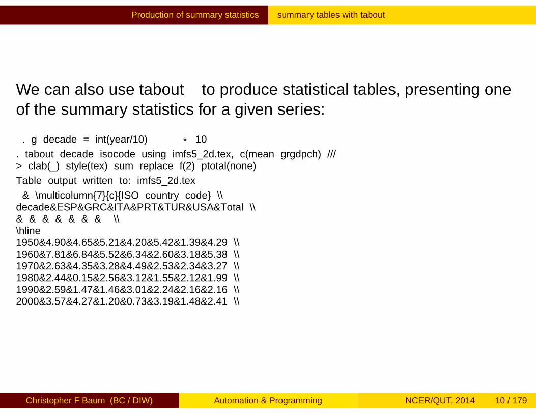
We can also use tabout to produce statistical tables, presenting oneof the summary statistics for a given series:
. g decade = int(year/10) * 10
. tabout decade isocode using imfs5_2d.tex, c(mean grgdpch) ///> clab(_) style(tex) sum replace f(2) ptotal(none)
Table output written to: imfs5_2d.tex
& \multicolumn{7}{c}{ISO country code} \\decade&ESP&GRC&ITA&PRT&TUR&USA&Total \\& & & & & & & \\\hline1950&4.90&4.65&5.21&4.20&5.42&1.39&4.29 \\1960&7.81&6.84&5.52&6.34&2.60&3.18&5.38 \\1970&2.63&4.35&3.28&4.49&2.53&2.34&3.27 \\1980&2.44&0.15&2.56&3.12&1.55&2.12&1.99 \\1990&2.59&1.47&1.46&3.01&2.24&2.16&2.16 \\2000&3.57&4.27&1.20&0.73&3.19&1.48&2.41 \\
Christopher F Baum (BC / DIW) Automation & Programming NCER/QUT, 2014 10 / 179
Production of summary statistics summary tables with tabout
Table 2. Average GDP per capita growth by decade, 1960–2007
ISO country codedecade ESP GRC ITA PRT TUR USA Total
1950 4.90 4.65 5.21 4.20 5.42 1.39 4.291960 7.81 6.84 5.52 6.34 2.60 3.18 5.381970 2.63 4.35 3.28 4.49 2.53 2.34 3.271980 2.44 0.15 2.56 3.12 1.55 2.12 1.991990 2.59 1.47 1.46 3.01 2.24 2.16 2.162000 3.57 4.27 1.20 0.73 3.19 1.48 2.41
1
Christopher F Baum (BC / DIW) Automation & Programming NCER/QUT, 2014 11 / 179
Production of summary statistics summary tables with estout
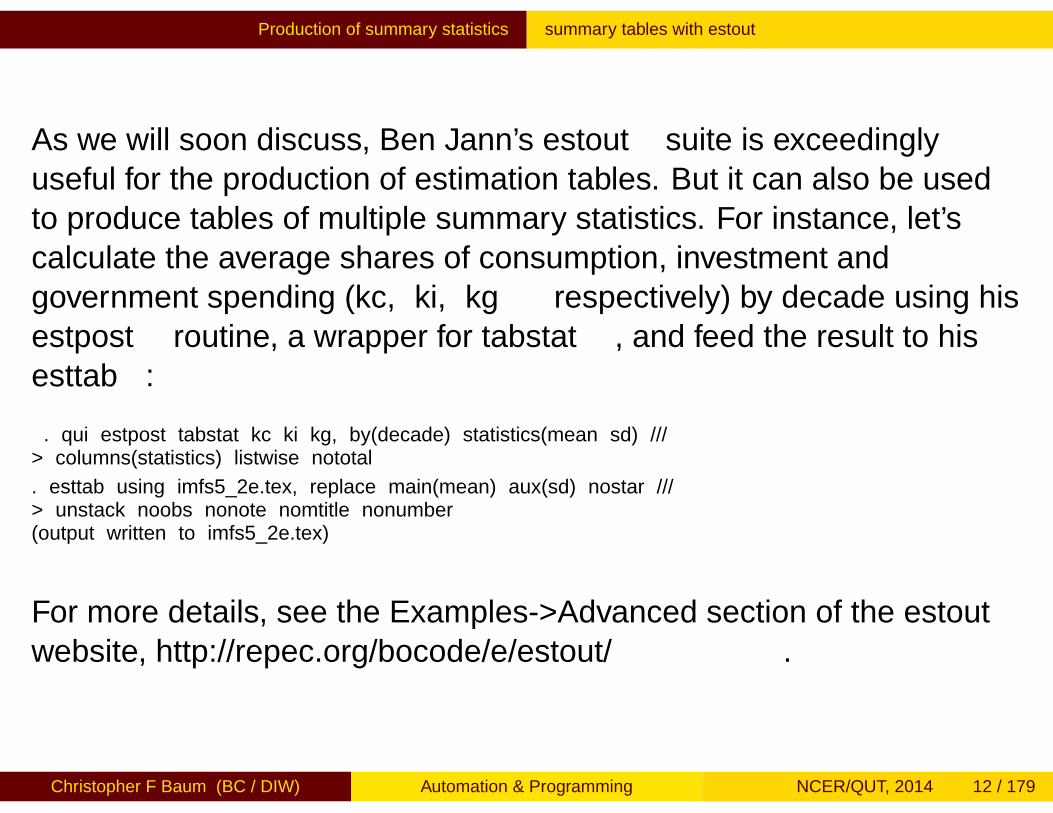
As we will soon discuss, Ben Jann’s estout suite is exceedinglyuseful for the production of estimation tables. But it can also be usedto produce tables of multiple summary statistics. For instance, let’scalculate the average shares of consumption, investment andgovernment spending (kc, ki, kg respectively) by decade using hisestpost routine, a wrapper for tabstat, and feed the result to hisesttab:
. qui estpost tabstat kc ki kg, by(decade) statistics(mean sd) ///> columns(statistics) listwise nototal
. esttab using imfs5_2e.tex, replace main(mean) aux(sd) nostar ///> unstack noobs nonote nomtitle nonumber(output written to imfs5_2e.tex)
For more details, see the Examples->Advanced section of the estoutwebsite, http://repec.org/bocode/e/estout/.
Christopher F Baum (BC / DIW) Automation & Programming NCER/QUT, 2014 12 / 179

Production of summary statistics summary tables with estout
Table 3. Average shares of consumption, investment, and government spending
1950 1960 1970 1980 1990 2000kc 67.15 62.49 61.69 62.64 62.24 61.49
(8.440) (8.226) (7.247) (5.512) (5.205) (5.350)
ki 21.60 27.41 28.68 24.96 27.81 31.24(6.234) (7.458) (7.205) (4.443) (4.104) (4.358)
kg 12.38 11.26 11.04 12.78 12.78 12.56(4.058) (2.604) (2.011) (1.701) (1.903) (2.367)
Note: Standard errors in parentheses.
1
Christopher F Baum (BC / DIW) Automation & Programming NCER/QUT, 2014 13 / 179

Production of estimates tables The estimates suite
Production of estimates tables
Stata has a suite of commands, estimates, that allow you to storesets of estimation results (and optionally save them to disk) so thatthey may be accessed later in either a statistical command (such ashausman) or, more commonly, to produce tables of estimates.
After any estimation (e-class) command, you may use estimatesstore setname to store that set of estimates for the duration of yourStata session. The setnames may then be used later in your do-file toaccess the stored estimates.
Christopher F Baum (BC / DIW) Automation & Programming NCER/QUT, 2014 14 / 179

Production of estimates tables The estimates suite
The estimates table command, which we have seen in earlierslides, can be used to produce a readable table of estimation resultsfrom several different models, with a number of options to control whatis presented (e.g., point estimates only, standard errors, t- orz-statistics, significance stars) and their format. The command canalso keep or drop certain coefficients (e.g., a set of time dummies)from the tabular output, and add a set of scalars to the table, includingAIC and BIC values.
Although this command was enhanced in recent versions of Stata, it isstill limited to producing a table in the results window and the logfile (ifopen). It does not support table export to other formats.
Christopher F Baum (BC / DIW) Automation & Programming NCER/QUT, 2014 15 / 179

Production of estimates tables estimates tables with estout
The estout command suite
To overcome these limitations, Ben Jann’s estout suite of programsprovides complete, easy-to-use routines to turn sets of estimates intopublication-quality tables in LATEX, MSWord or HTML formats. Theroutines have been described in two Stata Journal articles, 5:3 (2005)and 7:2 (2007), and estout has its own website:
http://repec.org/bocode/e/estout
which has explanations of all of the available options and numerousworked examples of its use.
Christopher F Baum (BC / DIW) Automation & Programming NCER/QUT, 2014 16 / 179

Production of estimates tables estimates tables with estout
To use the facilities of estout, you merely preface the estimationcommands with eststo:
eststo cleareststo: regress y x1 x2 x3eststo: probit z a1 a2 a3 a4eststo: ivreg2 y3 (y1 y2 = z1-z4) z5 z6, gmm2s
Then, to produce a table, just give command
esttab using myests.tex
which will create the LATEX table in that file. A file destined for Excelwould use the .csv extension; for MS Word, use .rtf. You may alsouse extension .html for HTML or .smcl for a table in Stata’s ownmarkup language.
Christopher F Baum (BC / DIW) Automation & Programming NCER/QUT, 2014 17 / 179

Production of estimates tables estimates tables with estout
The esttab command is a easy-to-use wrapper for estout, whichhas many options to control the exact format and content of the table.Any of the estout options may be used in the esttab command. Forinstance, you may want to suppress the coefficient listings of yeardummies in a panel regression.
You may also use estadd to include user-generated statistics in theereturn list (such as elasticities produced by margins) so thatthey can be accessed by esttab.
Christopher F Baum (BC / DIW) Automation & Programming NCER/QUT, 2014 18 / 179

Production of estimates tables estimates tables with estout
It may be necessary to change the format of your estimation tableswhen submitting a paper to a different journal: for instance, one whichwants t-statistics rather than standard errors reported. This may beeasily achieved by just rerunning the estimation job with differentestout options.
Christopher F Baum (BC / DIW) Automation & Programming NCER/QUT, 2014 19 / 179
Production of estimates tables estimates tables with estout
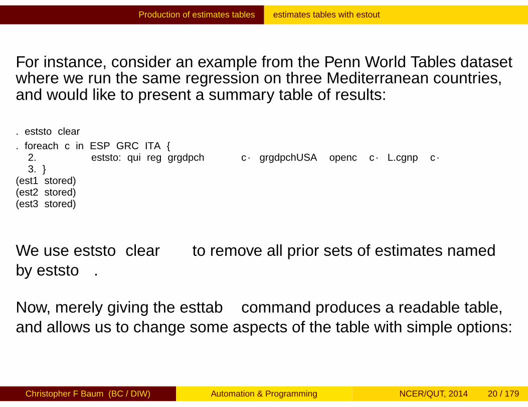
For instance, consider an example from the Penn World Tables datasetwhere we run the same regression on three Mediterranean countries,and would like to present a summary table of results:
. eststo clear
. foreach c in ESP GRC ITA {2. eststo: qui reg grgdpch`c´ grgdpchUSA openc`c´ L.cgnp`c´3. }
(est1 stored)(est2 stored)(est3 stored)
We use eststo clear to remove all prior sets of estimates namedby eststo.
Now, merely giving the esttab command produces a readable table,and allows us to change some aspects of the table with simple options:
Christopher F Baum (BC / DIW) Automation & Programming NCER/QUT, 2014 20 / 179

Production of estimates tables estimates tables with estout
. esttab, drop(_cons) stat(r2 rmse)
(1) (2) (3)grgdpchESP grgdpchGRC grgdpchITA
grgdpchUSA 0.279 0.358 0.149(1.42) (1.71) (1.02)
opencESP -0.0207(-0.50)
L.cgnpESP 2.058(1.62)
opencGRC -0.211***(-4.56)
L.cgnpGRC -1.351**(-3.26)
opencITA -0.0672(-1.60)
L.cgnpITA 1.353*(2.53)
r2 0.152 0.425 0.296rmse 3.051 3.173 2.236
t statistics in parentheses
* p<0.05, ** p<0.01, *** p<0.001
Christopher F Baum (BC / DIW) Automation & Programming NCER/QUT, 2014 21 / 179

Production of estimates tables estimates tables with estout
By providing variable labels and using a few additional esttaboptions, we can make the table more readable:. esttab, drop(_cons) se stat(r2 rmse) lab nonum ti("GDP growth regressions")
GDP growth regressions
ESP GRC ITA
US gdp gr 0.279 0.358 0.149(0.196) (0.209) (0.146)
ESP openness -0.0207(0.0411)
L.ESP rgdp per cap. 2.058(1.267)
GRC openness -0.211***(0.0463)
L.GRC rgdp per cap. -1.351**(0.415)
ITA openness -0.0672(0.0419)
L.ITA rgdp per cap. 1.353*(0.534)
r2 0.152 0.425 0.296rmse 3.051 3.173 2.236
Standard errors in parentheses
* p<0.05, ** p<0.01, *** p<0.001
Christopher F Baum (BC / DIW) Automation & Programming NCER/QUT, 2014 22 / 179

Production of estimates tables estimates tables with estout
Still, this is merely a SMCL-format table in Stata’s results window, andsomething we could have probably produced with estimatestable. The usefulness of the estout suite comes from its ability toproduce the tables in other output formats. For example:
. esttab using imfs5_1d.rtf, replace drop(_cons) se stat(r2 rmse) ///> lab nonum ti("GDP growth regressions, 1960-2007")(note: file imfs5_1d.rtf not found)(output written to imfs5_1d.rtf)
Which, when opened in MS Word or OpenOffice, yields
Christopher F Baum (BC / DIW) Automation & Programming NCER/QUT, 2014 23 / 179

Production of estimates tables estimates tables with estout
GDP growth regressions, 1960-2007ESP GRC ITA
US gdp gr 0.279 0.358 0.149(0.196) (0.209) (0.146)
ESP openness -0.0207(0.0411)
L.ESP rgdp per cap. 2.058(1.267)
GRC openness -0.211***
(0.0463)
L.GRC rgdp per cap. -1.351**
(0.415)
ITA openness -0.0672(0.0419)
L.ITA rgdp per cap. 1.353*
(0.534)r2 0.152 0.425 0.296rmse 3.051 3.173 2.236Standard errors in parentheses* p < 0.05, ** p < 0.01, *** p < 0.001
1
Christopher F Baum (BC / DIW) Automation & Programming NCER/QUT, 2014 24 / 179

Production of estimates tables adding statistics with estadd
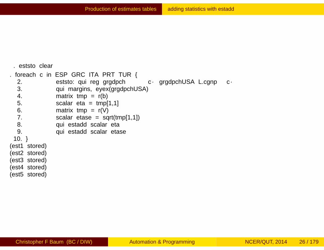
Let us illustrate how additional statistics may be added to a table.Consider the prior regressions (dropping the openness measure, andadding two additional countries) where we use margins to computethe elasticity of each country’s GDP growth with respect to US GDPgrowth. By default, margins is a r-class command, so it returns theelasticity in matrix r(b) and its estimated variance in r(V).
As an aside, margins can also be used as an e-class command byinvoking the post option. This example would be somewhat morecomplicated in that case, as we would have two e-class commandsfrom which various results are to be combined.
Christopher F Baum (BC / DIW) Automation & Programming NCER/QUT, 2014 25 / 179
Production of estimates tables adding statistics with estadd
. eststo clear
. foreach c in ESP GRC ITA PRT TUR {2. eststo: qui reg grgdpch`c´ grgdpchUSA L.cgnp`c´3. qui margins, eyex(grgdpchUSA)4. matrix tmp = r(b)5. scalar eta = tmp[1,1]6. matrix tmp = r(V)7. scalar etase = sqrt(tmp[1,1])8. qui estadd scalar eta9. qui estadd scalar etase
10. }(est1 stored)(est2 stored)(est3 stored)(est4 stored)(est5 stored)
Christopher F Baum (BC / DIW) Automation & Programming NCER/QUT, 2014 26 / 179

Production of estimates tables estout and LATEX
The greatest degree of automation, using estout, arises when usingit to produce LATEX tables. As LATEX is a programming language as well,estout can be instructed to include, for instance, Greek symbols,sub- and superscripts, and the like in its output, which will thenproduce a beautifully formatted table, ready for inclusion in apublication. In fact, camera-ready copy for Stata Press books, such asthose I have authored, is produced in that manner.
. esttab using imfs5_1f.tex, replace drop(_cons) se lab nonum ///> ti("GDP growth regressions, 1960-2007") stat(eta etase r2 rmse, ///> labels("\$\hat{\eta}\$" "s.e." "\$R^2\$" "\$RMSE\$")) ///> note("Note: \$\eta\$: elasticity of GDP growth w.r.t. US GDP growth")(output written to imfs5_1f.tex)
In this example, I have inserted LATEX typesetting commands to labelstatistics as you might choose to label them in a journal submission.
Christopher F Baum (BC / DIW) Automation & Programming NCER/QUT, 2014 27 / 179

Production of estimates tables estout and LATEX
Table 2. GDP growth regressions, 1960-2007
ESP GRC ITA PRT TURUS GDP growth 0.291 0.577∗ 0.193 0.439 0.331
(0.193) (0.245) (0.146) (0.284) (0.309)
L.ESP RGDP p/c 2.400∗
(1.061)
L.GRC RGDP p/c -0.770(0.475)
L.ITA RGDP p/c 1.716∗∗
(0.492)
L.PRT RGDP p/c 0.499(0.366)
L.TUR RGDP p/c -0.577(1.036)
η̂ 0.151 0.869 0.386 0.380 0.150s.e. 0.0397 43.04 0.636 0.939 0.180R2 0.147 0.146 0.254 0.0881 0.0390RMSE 3.025 3.822 2.276 4.452 4.382
Note: η: elasticity of GDP growth w.r.t. US GDP growth∗ p < 0.05, ∗∗ p < 0.01, ∗∗∗ p < 0.001
1
Christopher F Baum (BC / DIW) Automation & Programming NCER/QUT, 2014 28 / 179
Production of estimates tables estout and LATEX
In a slightly more elaborate example, consider modelling theprobability that GDP growth will exceed its historical median value,using a binomial probit model. In such a model, we do not want toreport the original coefficients, which are marginal effects on the latentvariable, but rather their transformations as measures of the effects onthe probability of high GDP growth.
In this context, we estimate the model for each country, use marginsto produce its default dydx values of ∂Pr [·]/∂X , and use the postoption to store those as e-returns, to be captured by eststo. We alsostore the median growth rate so that it can be reported in the table.
Christopher F Baum (BC / DIW) Automation & Programming NCER/QUT, 2014 29 / 179

Production of estimates tables estout and LATEX
. eststo clear
. foreach c in ESP GRC ITA PRT TUR {2. qui summ grgdpch`c´, detail3. scalar medgro`c´ = r(p50)4. g higrowth`c´ = (grgdpch`c´ > medgro`c´)5. lab var higrowth`c´ "`c´"6. qui probit higrowth`c´ grgdpchUSA L.cgnp`c´, nolog7. qui eststo: margins, dydx(*) post8. qui estadd scalar medgro = medgro`c´9. }
. esttab using imfs5_1h.tex, replace se lab nonum ///> ti("Pr[GDP growth \$>\$ median], 1960-2007") stat(medgro, ///> labels("Median growth rate")) mti("ESP" "GRC" "ITA" "PRT" "TUR") ///> note("Note: Marginal effects (\$\partial Pr[\cdot]/\partial X\$ displayed")(output written to imfs5_1h.tex)
Christopher F Baum (BC / DIW) Automation & Programming NCER/QUT, 2014 30 / 179

Production of estimates tables estout and LATEX
Table 1. Pr[GDP growth > median], 1960-2007
ESP GRC ITA PRT TURUS GDP growth 0.0566∗ 0.0309 0.0239 0.0482 0.0566
(0.0278) (0.0292) (0.0288) (0.0291) (0.0321)
L.ESP RGDP p/c 0.299∗
(0.151)
L.GRC RGDP p/c -0.150∗∗
(0.0529)
L.ITA RGDP p/c 0.292∗∗∗
(0.0775)
L.PRT RGDP p/c 0.0507(0.0380)
L.TUR RGDP p/c -0.124(0.109)
Median growth rate 3.553 3.495 2.473 3.671 3.156
Note: Marginal effects (∂Pr[·]/∂X displayed∗ p < 0.05, ∗∗ p < 0.01, ∗∗∗ p < 0.001
1
Christopher F Baum (BC / DIW) Automation & Programming NCER/QUT, 2014 31 / 179

Production of sets of tables and graphs
Production of sets of tables and graphs
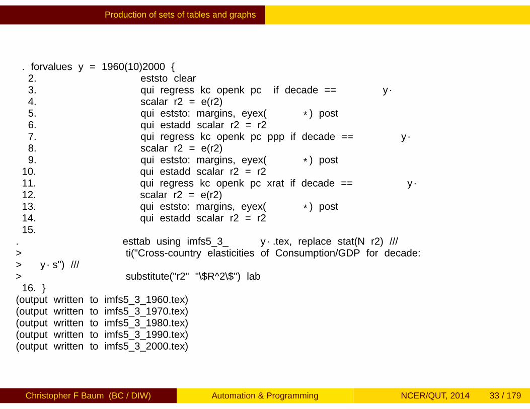
You may often have the need to produce a sizable number of verysimilar tables or graphs: one per country, sector or industry, or one peryear, quinquennium or decade. We first illustrate how that might beautomated for a set of regression tables: in this case, cross-countryregressions over several decades, one table per decade.
. use pwt6_3, clear(Penn World Tables 6.3, August 2009)
. keep if inlist(isocode, "ITA", "ESP", "GRC", "PRT", "BEL", ///> "FRA", "ITA", "GER", "DNK")(10556 observations deleted)
. g decade = int(year/10) * 10
Christopher F Baum (BC / DIW) Automation & Programming NCER/QUT, 2014 32 / 179
Production of sets of tables and graphs
. forvalues y = 1960(10)2000 {2. eststo clear3. qui regress kc openk pc if decade == `y´4. scalar r2 = e(r2)5. qui eststo: margins, eyex(*) post6. qui estadd scalar r2 = r27. qui regress kc openk pc ppp if decade == `y´8. scalar r2 = e(r2)9. qui eststo: margins, eyex(*) post
10. qui estadd scalar r2 = r211. qui regress kc openk pc xrat if decade == `y´12. scalar r2 = e(r2)13. qui eststo: margins, eyex(*) post14. qui estadd scalar r2 = r215.
. esttab using imfs5_3_`y´.tex, replace stat(N r2) ///> ti("Cross-country elasticities of Consumption/GDP for decade:> `y´s") ///> substitute("r2" "\$R^2\$") lab16. }(output written to imfs5_3_1960.tex)(output written to imfs5_3_1970.tex)(output written to imfs5_3_1980.tex)(output written to imfs5_3_1990.tex)(output written to imfs5_3_2000.tex)
Christopher F Baum (BC / DIW) Automation & Programming NCER/QUT, 2014 33 / 179

Production of sets of tables and graphs
We can then include the separate LATEX tables produced by the do-filein a research paper with the commands:
\input{imfs5_3_1960}\input{imfs5_3_1970}
etc.
This approach has the advantage that the tables themselves need notbe included in the document, so if we revise the tables we need notcopy and paste the tables. There may be a similar capability availableusing RTF tables. To illustrate, here is one of the tables produced bythis do-file:
Christopher F Baum (BC / DIW) Automation & Programming NCER/QUT, 2014 34 / 179

Production of sets of tables and graphs
Table 4. Cross-country elasticities of Consumption/GDP for decade: 1970s
(1) (2) (3)
Openness in constant prices -0.0113 -0.0137 -0.0134(-0.86) (-1.03) (-1.02)
Price level of consumption -0.0430 -0.0162 -0.0168(-1.44) (-0.41) (-0.47)
Purchasing power parity -0.00679(-1.03)
Exchange rate vs USD -0.00885(-1.31)
N 80 80 80R2 0.0550 0.0685 0.0765
t statistics in parentheses∗ p < 0.05, ∗∗ p < 0.01, ∗∗∗ p < 0.001
1
Christopher F Baum (BC / DIW) Automation & Programming NCER/QUT, 2014 35 / 179
Production of sets of tables and graphs graphics automation
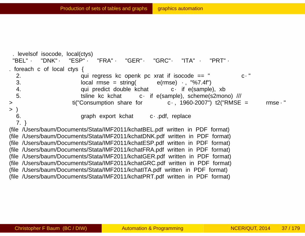
Likewise, we could automate the production of a set of very similargraphs. Graphics automation is very valuable, as it avoids the manualtweaking of graphs produced by other software by making it a purelyprogrammable function. Although the Stata graphics language iscomplex, the desired graph can be built up with the options needed toproduce exactly the right appearance.
As an example, consider automating a plot of the actual and predictedvalues for time-series regressions for each country in this sample:
Christopher F Baum (BC / DIW) Automation & Programming NCER/QUT, 2014 36 / 179
Production of sets of tables and graphs graphics automation
. levelsof isocode, local(ctys)`"BEL"´ `"DNK"´ `"ESP"´ `"FRA"´ `"GER"´ `"GRC"´ `"ITA"´ `"PRT"´
. foreach c of local ctys {2. qui regress kc openk pc xrat if isocode == "`c´"3. local rmse = string(`e(rmse)´, "%7.4f")4. qui predict double kchat`c´ if e(sample), xb5. tsline kc kchat`c´ if e(sample), scheme(s2mono) ///
> ti("Consumption share for `c´, 1960-2007") t2("RMSE = `rmse´"> )
6. graph export kchat`c´.pdf, replace7. }
(file /Users/baum/Documents/Stata/IMF2011/kchatBEL.pdf written in PDF format)(file /Users/baum/Documents/Stata/IMF2011/kchatDNK.pdf written in PDF format)(file /Users/baum/Documents/Stata/IMF2011/kchatESP.pdf written in PDF format)(file /Users/baum/Documents/Stata/IMF2011/kchatFRA.pdf written in PDF format)(file /Users/baum/Documents/Stata/IMF2011/kchatGER.pdf written in PDF format)(file /Users/baum/Documents/Stata/IMF2011/kchatGRC.pdf written in PDF format)(file /Users/baum/Documents/Stata/IMF2011/kchatITA.pdf written in PDF format)(file /Users/baum/Documents/Stata/IMF2011/kchatPRT.pdf written in PDF format)
Christopher F Baum (BC / DIW) Automation & Programming NCER/QUT, 2014 37 / 179

Production of sets of tables and graphs graphics automation
5556
5758
5960
1940 1960 1980 2000 2020year
Consumption / Real GDP Linear prediction
RMSE = 1.1744Consumption share for FRA, 1960-2007
Christopher F Baum (BC / DIW) Automation & Programming NCER/QUT, 2014 38 / 179
Production of sets of tables and graphs graphics automation
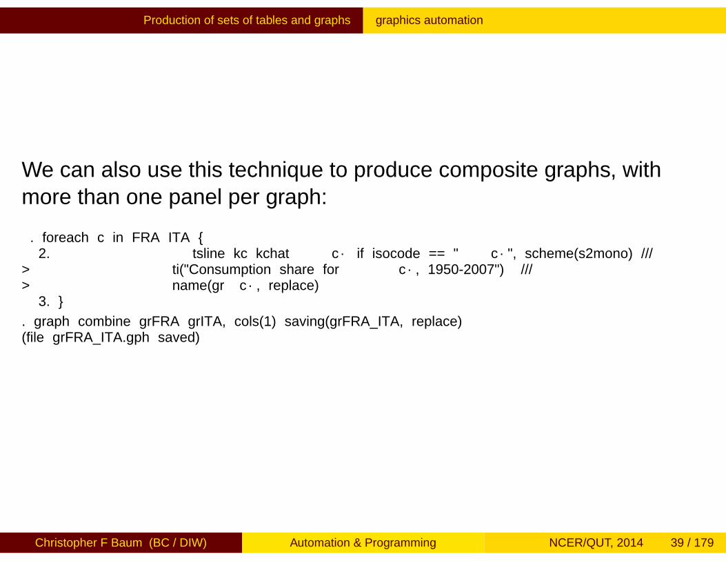
We can also use this technique to produce composite graphs, withmore than one panel per graph:
. foreach c in FRA ITA {2. tsline kc kchat`c´ if isocode == "`c´", scheme(s2mono) ///
> ti("Consumption share for `c´, 1950-2007") ///> name(gr`c´, replace)
3. }
. graph combine grFRA grITA, cols(1) saving(grFRA_ITA, replace)(file grFRA_ITA.gph saved)
Christopher F Baum (BC / DIW) Automation & Programming NCER/QUT, 2014 39 / 179

Production of sets of tables and graphs graphics automation
5556
5758
5960
1940 1960 1980 2000 2020year
Consumption / Real GDP Linear prediction
Consumption share for FRA, 1950-2007
4850
5254
5658
1940 1960 1980 2000 2020year
Consumption / Real GDP Linear prediction
Consumption share for ITA, 1950-2007
Christopher F Baum (BC / DIW) Automation & Programming NCER/QUT, 2014 40 / 179

Should you be a Stata programmer?
Should you be a Stata programmer?
We now turn to the broader question: how advantageous might it be toacquire Stata programming skills? First, some nomenclature related toprogramming:
You should consider yourself a Stata programmer if you writedo-files: sequences of Stata commands which you execute withthe do command or by double-clicking on the file.You might also write what Stata formally defines as a program: aset of Stata commands that includes the program statement. AStata program, stored in an ado-file, defines a new Statacommand.You may use Stata’s programming language, Mata, to writeroutines in that language that are called by ado-files.
Christopher F Baum (BC / DIW) Automation & Programming NCER/QUT, 2014 41 / 179

Should you be a Stata programmer?
Any of these tasks involve Stata programming.
With that set of definitions in mind, we must deal with the why: whyshould you become a Stata programmer? After answering thatessential question, we take up some of the aspects of how: how youcan become a more efficient user of Stata by making use ofprogramming techniques, be they simple or complex.
Christopher F Baum (BC / DIW) Automation & Programming NCER/QUT, 2014 42 / 179

Should you be a Stata programmer?
Using any computer program or language is all about efficiency: notcomputational efficiency as much as human efficiency. You want thecomputer to do the work that can be routinely automated, allowing youto make more efficient use of your time and reducing human errors.Computers are excellent at performing repetitive tasks; humans arenot.
One of the strongest rationales for learning how to use programmingtechniques in Stata is the potential to shift more of the repetitiveburden of data management, statistical analysis and the production ofgraphics to the computer.
Let’s consider several specific advantages of using Stata programmingtechniques in the three contexts enumerated above.
Christopher F Baum (BC / DIW) Automation & Programming NCER/QUT, 2014 43 / 179

Should you be a Stata programmer? Using do-files
Context 1: do-file programming
Using a do-file to automate a specific data management or statisticaltask leads to reproducible research and the ability to document theempirical research process. This reduces the effort needed to performa similar task at a later point, or to document the specific steps youfollowed for your co-workers.
Ideally, your entire research project should be defined by a set ofdo-files which execute every step from input of the raw data toproduction of the final tables and graphs. As a do-file can call anotherdo-file (and so on), a hierarchy of do-files can be used to handle aquite complex project.
Christopher F Baum (BC / DIW) Automation & Programming NCER/QUT, 2014 44 / 179

Should you be a Stata programmer? Using do-files
The beauty of this approach is flexibility: if you find an error in anearlier stage of the project, you need only modify the code and rerunthat do-file and those following to bring the project up to date. Forinstance, an researcher may need to respond to a review of herpaper—submitted months ago to an academic journal—by revising thespecification of variables in a set of estimated models and estimatingnew statistical results. If all of the steps producing the final results aredocumented by a set of do-files, that task becomes straightforward.
I argue that all serious users of Stata should gain some facility withdo-files and the Stata commands that support repetitive use ofcommands. A few hours’ investment should save days of weeks oftime over the course of a sizable research project.
Christopher F Baum (BC / DIW) Automation & Programming NCER/QUT, 2014 45 / 179

Should you be a Stata programmer? Using do-files
That advice does not imply that Stata’s interactive capabilities shouldbe shunned. Stata is a powerful and effective tool for exploratory dataanalysis and ad hoc queries about your data. But data managementtasks and the statistical analyses leading to tabulated results shouldnot be performed with “point-and-click” tools which leave you withoutan audit trail of the steps you have taken.
Responsible research involves reproducibility, and “point-and-click”tools do not promote reproducibility. For that reason, I counselresearchers to move their data into Stata (from a spreadsheetenvironment, for example) as early as possible in the process, andperform all transformations, data cleaning, etc. with Stata’s do-filelanguage. This can save a great deal of time when mistakes aredetected in the raw data, or when they are revised.
Christopher F Baum (BC / DIW) Automation & Programming NCER/QUT, 2014 46 / 179
Should you be a Stata programmer? Writing your own ado-files
Context 2: ado-file programming
You may find that despite the breadth of Stata’s official and user-writencommands, there are tasks that you must repeatedly perform thatinvolve variations on the same do-file. You would like Stata to have acommand to perform those tasks. At that point, you should considerStata’s ado-file programming capabilities.
Christopher F Baum (BC / DIW) Automation & Programming NCER/QUT, 2014 47 / 179
Should you be a Stata programmer? Writing your own ado-files
Stata has great flexibility: a Stata command need be no more than afew lines of Stata code, and once defined that command becomes a“first-class citizen." You can easily write a Stata program, stored in anado-file, that handles all the features of official Stata commands suchas if exp, in range and command options. You can (and should)write a help file that documents its operation for your benefit and forthose with whom you share the code.
Although ado-file programming requires that you learn how to usesome additional commands used in that context, it may help youbecome more efficient in performing the data management, statisticalor graphical tasks that you face.
Christopher F Baum (BC / DIW) Automation & Programming NCER/QUT, 2014 48 / 179

Should you be a Stata programmer? Writing your own ado-files
My first response to would-be ado-file programmers: don’t! In manycases, standard Stata commands will perform the tasks you need. Abetter understanding of the capabilities of those commands will oftenlead to a researcher realizing that a combination of Stata commandswill do the job nicely, without the need for custom programming.
Those familiar with other statistical packages or computer languagesoften see the need to write a program to perform a task that can behandled with some of Stata’s unique constructs: the local macro andthe functions available for handling macros and lists. If you becomefamiliar with those tools, as well as the full potential of commands suchas merge, you may recognize that your needs can be readily met.
Christopher F Baum (BC / DIW) Automation & Programming NCER/QUT, 2014 49 / 179

Should you be a Stata programmer? Writing your own ado-files
The second bit of advice along those lines: use Stata’s searchcommand and the Stata user community (via Statalist) to ensure thatthe program you envision writing has not already been written. In manycases an official Stata command will do almost what you want, andyou can modify (and rename) a copy of that command to add thefeatures you need.
In other cases, a user-written program from the Stata Journal or theSSC Archive (help ssc) may be close to what you need. You caneither contact its author or modify (and rename) a copy of thatcommand to meet your needs.
In either case, the bottom line is the same advice:don’t waste your time reinventing the wheel!
Christopher F Baum (BC / DIW) Automation & Programming NCER/QUT, 2014 50 / 179
Should you be a Stata programmer? Writing your own ado-files
If your particular needs are not met by existing Stata commands nor byuser-written software, and they involve a general task, you shouldconsider writing your own ado-file. In contrast to many statisticalprogramming languages and software environments, Stata makes itvery easy to write new commands which implement all of Stata’sfeatures and error-checking tools. Some investment in the ado-filelanguage is needed, but a good understanding of the features of thatlanguage—such as the program and syntax statements—is nothard to develop.
Christopher F Baum (BC / DIW) Automation & Programming NCER/QUT, 2014 51 / 179
Should you be a Stata programmer? Writing your own ado-files
A huge benefit accrues to the ado-file author: few data management,statistical, tabulation or graphical tasks are unique. Once you developan ado-file to perform a particular task, you will probably run acrossanother task that is quite similar. A clone of the ado-file, customized forthe new task, will often suffice.
In this context, ado-file programming allows you to assemble aworkbench of tools where most of the associated cost is learning howto build the first few tools.
Christopher F Baum (BC / DIW) Automation & Programming NCER/QUT, 2014 52 / 179

Should you be a Stata programmer? Writing your own ado-files
Another rationale for many researchers to develop limited fluency inStata’s ado-file language:
Stata’s maximum likelihood (ml) capabilities usually involve theconstruction of an ado-file program defining the likelihood function.The simulate, bootstrap and jackknife commands may beused with standard Stata commands, but in many cases mayrequire that a command be constructed to produce the neededresults for each repetition.Although the nonlinear least squares commands (nl, nlsur) andthe GMM command (gmm) may be used in an interactive mode, it islikely that a Stata program will often be the easiest way to performany complex NLLS or GMM task.
Christopher F Baum (BC / DIW) Automation & Programming NCER/QUT, 2014 53 / 179

Should you be a Stata programmer? Writing Mata subroutines for ado-files
Context 3: Mata subroutines for ado-files
Your ado-files may perform some complicated tasks which involvemany invocations of the same commands. Stata’s ado-file language iseasy to read and write, but it is interpreted: Stata must evaluate eachstatement and translate it into machine code. Stata’s Mataprogramming language (help mata) creates compiled code whichcan run much faster than ado-file code.
Your ado-file can call a Mata routine to carry out a computationallyintensive task and return the results in the form of Stata variables,scalars or matrices. Although you may think of Mata solely as a “matrixlanguage”, it is actually a general-purpose programming language,suitable for many non-matrix-oriented tasks such as text processingand list management.
Christopher F Baum (BC / DIW) Automation & Programming NCER/QUT, 2014 54 / 179

Should you be a Stata programmer? Writing Mata subroutines for ado-files
The Mata programming environment is tightly integrated with Stata,allowing interchange of variables, local and global macros and Statamatrices to and from Mata without the necessity to make copies ofthose objects. A Mata program can easily generate an entire set ofnew variables (often in one matrix operation), and those variables willbe available to Stata when the Mata routine terminates.
Mata’s similarity to the C language makes it very easy to use foranyone with prior knowledge of C. Its handling of matrices is broadlysimilar to the syntax of other matrix programming languages such asMATLAB, Ox and Gauss. Translation of existing code for thoselanguages or from lower-level languages such as Fortran or C isusually quite straightforward. Unlike Stata’s C plugins, code in Mata isplatform-independent, and developing code in Mata is easier than incompiled C.
Christopher F Baum (BC / DIW) Automation & Programming NCER/QUT, 2014 55 / 179
Tools for do-file authors
Tools for do-file authors
In this section of the talk, I will mention a number of tools and tricksuseful for do-file authors. Like any language, the Stata do-file languagecan be used eloquently or incoherently. Users who bring otherlanguages’ techniques and try to reproduce them in Stata often findthat their Stata programs resemble Google’s automated translation ofGerman to English: possibly comprehensible, but a long way fromwhat a native speaker would say. We present suggestions on how thelanguage may be used most effectively.
Although I focus on authoring do-files, these tips are equally useful forado-file authors: and perhaps even more important in that context, asan ado-file program may be run many times.
Christopher F Baum (BC / DIW) Automation & Programming NCER/QUT, 2014 56 / 179

Tools for do-file authors Looping over observations is rarely appropriate
Looping over observations is rarely appropriate
One of the important metaphors of Stata usage is that commandsoperate on the entire data set unless otherwise specified. There israrely any reason to explicitly loop over observations. Constructswhich would require looping in other programming languages aregenerally single commands in Stata: e.g., recode.
For example: do not use the “programmer’s if” on Stata variables!For example,
if (race == 1) {(calculate something)
} else if (race == 2) {...
will not do what you expect. It will examine the value of race in thefirst observation of the data set, not in each observation in turn! In thiscase the if qualifier should be used.
Christopher F Baum (BC / DIW) Automation & Programming NCER/QUT, 2014 57 / 179
Tools for do-file authors The by prefix can often replace a loop
The by prefix can often replace a loop
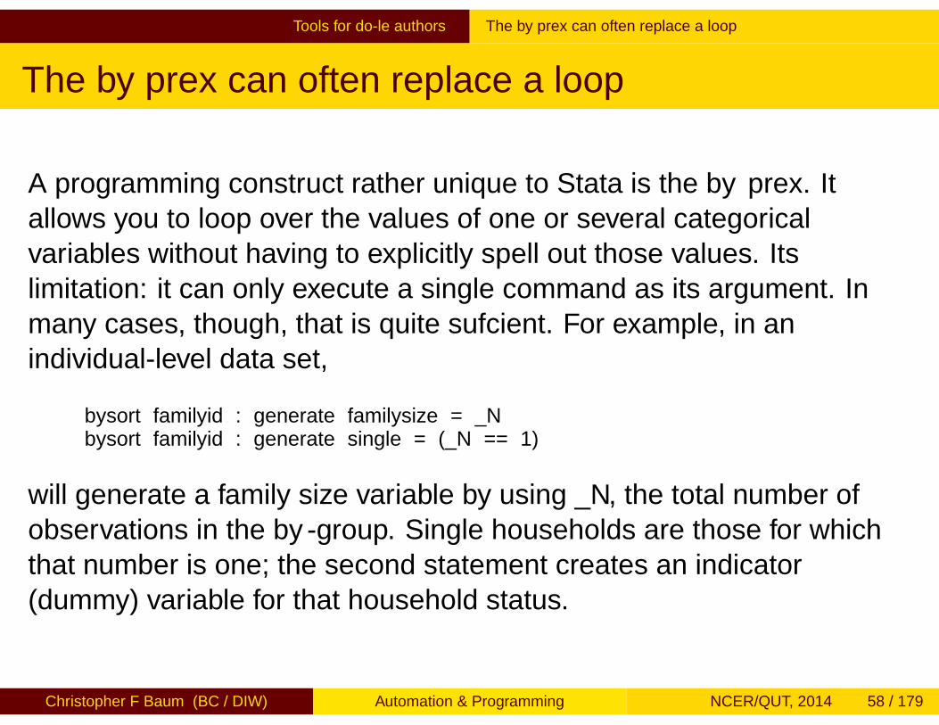
A programming construct rather unique to Stata is the by prefix. Itallows you to loop over the values of one or several categoricalvariables without having to explicitly spell out those values. Itslimitation: it can only execute a single command as its argument. Inmany cases, though, that is quite sufficient. For example, in anindividual-level data set,
bysort familyid : generate familysize = _Nbysort familyid : generate single = (_N == 1)
will generate a family size variable by using _N, the total number ofobservations in the by-group. Single households are those for whichthat number is one; the second statement creates an indicator(dummy) variable for that household status.
Christopher F Baum (BC / DIW) Automation & Programming NCER/QUT, 2014 58 / 179
Tools for do-file authors Repeated statements are usually not needed
Repeated statements are usually not needed
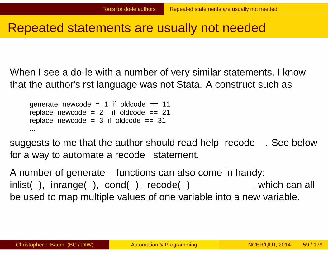
When I see a do-file with a number of very similar statements, I knowthat the author’s first language was not Stata. A construct such as
generate newcode = 1 if oldcode == 11replace newcode = 2 if oldcode == 21replace newcode = 3 if oldcode == 31...
suggests to me that the author should read help recode. See belowfor a way to automate a recode statement.
A number of generate functions can also come in handy:inlist( ), inrange( ), cond( ), recode( ), which can allbe used to map multiple values of one variable into a new variable.
Christopher F Baum (BC / DIW) Automation & Programming NCER/QUT, 2014 59 / 179

Tools for do-file authors Merge can solve concordance problems
Merge can solve concordance problems
A more general technique to solve concordance problems is offered bymerge. If you want to map (or concord) values into a particularscheme—for instance, associate the average income in a postal codewith all households whose address lies in that code—do not usecommands to define that mapping. Construct a separate data set,containing the postal code and average income value (and any otheravailable measurements) and merge it with the household-level dataset:
merge n:1 postalcode using pcstats
where the n:1 clause specifies that the postal-code file must haveunique entries of that variable. If additional information is available atthe postal code level, you may just add it to the using file and run themerge again. One merge command replaces many explicit generateand replace commands.
Christopher F Baum (BC / DIW) Automation & Programming NCER/QUT, 2014 60 / 179

Tools for do-file authors Some simple commands are often overlooked
Some simple commands are often overlooked
Nick Cox’s Speaking Stata column in the Stata Journal has pointed outseveral often-overlooked but very useful commands. For instance, thecount command can be used to determine, in ad hoc interactive useor in a do-file, how many observations satisfy a logical condition. Fordo-file authors, the assert command may be used to ensure that anecessary condition is satisfied: e.g.
assert gender == 1 | gender == 2
will bring the do-file to a halt if that condition fails. This is a very usefultool to both validate raw data and ensure that any transformationshave been conducted properly.
Duplicate entries in certain variables may be logically impossible. Howcan you determine whether they exist, and if so, deal with them? Theduplicates suite of commands provides a comprehensive set oftools for dealing with duplicate entries.
Christopher F Baum (BC / DIW) Automation & Programming NCER/QUT, 2014 61 / 179

Tools for do-file authors egen functions can solve many programming problems
egen functions can solve many programmingproblems
Every do-file author should be familiar with [D] functions(functions for generate) and [D] egen. The list of official egenfunctions includes many tools which you may find very helpful: forinstance, a set of row-wise functions that allow you to specify a list ofvariables, which mimic similar functions in a spreadsheet environment.Matching functions such as anycount, anymatch, anyvalueallow you to find matching values in a varlist. Statistical egenfunctions allow you to compute various statistics as new variables:particularly useful in conjunction with the by-prefix, as we will discuss.
In addition, the list of egen functions is open-ended: many user-writtenfunctions are available in the SSC Archive (notably, Nick Cox’segenmore), and you can write your own.
Christopher F Baum (BC / DIW) Automation & Programming NCER/QUT, 2014 62 / 179

Tools for do-file authors Learn how to use return and ereturn
Learn how to use return and ereturn
Almost all Stata commands return their results in the return list or theereturn list. These returned items are categorized as macros, scalarsor matrices. Your do-file may make use of any information left behindas long as you understand how to save it for future use and refer to it inyour do-file. For instance, highlighting the use of assert:
summarize region, meanonlyassert r(min) > 0 & r(max) < 5
will validate the values of region in the data set to ensure that theyare valid. summarize is an r-class command, and returns its results inr( ) items. Estimation commands, such as regress or probit,return their results in the ereturn list. For instance, e(r2) is theregression R2, and matrix e(b) is the row vector of estimatedcoefficients.
Christopher F Baum (BC / DIW) Automation & Programming NCER/QUT, 2014 63 / 179

Tools for do-file authors Learn how to use return and ereturn
The values from the return list and ereturn list may be usedin computations:
summarize famsize, detailscalar iqr = r(p75) - r(p25)scalar semean = r(sd) / sqrt(r(N))display "IQR : " iqrdisplay "mean : " r(mean) " s.e. : " semean
will compute and display the inter-quartile range and the standard errorof the mean of famsize. Here we have used Stata’s scalars tocompute and store numeric values.
In Stata, the scalar plays the role of a “variable” in a traditionalprogramming language.
Christopher F Baum (BC / DIW) Automation & Programming NCER/QUT, 2014 64 / 179

Tools for do-file authors extended macro functions, list functions, levelsof
extended macro functions, list functions, levelsof
Beyond their use in loop constructs with foreach, local macros canalso be manipulated with an extensive set of extended macro functionsand list functions. These functions (described in [P] macro and [P]macro lists) can be used to count the number of elements in amacro, extract each element in turn, extract the variable label or valuelabel from a variable, or generate a list of files that match a particularpattern.
A number of string functions are available in [D] functions toperform string manipulation tasks found in other string processinglanguages (including support for regular expressions, or regexps.)
Christopher F Baum (BC / DIW) Automation & Programming NCER/QUT, 2014 65 / 179

Tools for do-file authors extended macro functions, list functions, levelsof
A very handy command that produces a macro is levelsof, whichreturns a sorted list of the distinct values of varname, optionally as amacro. This list would be used in a by-prefix expression automatically,but what if you want to issue several commands rather than one? Thena foreach, using the local macro created by levelsof, is thesolution.
Christopher F Baum (BC / DIW) Automation & Programming NCER/QUT, 2014 66 / 179
Ado-file programming: a primer The program statement
Ado-file programming: a primer
Continuing in our trinity of Stata programming roles, let us now discussthe rudiments of ado-file programming.
A Stata program adds a command to Stata’s language. The name ofthe program is the command name, and the program must be stored ina file of that same name with extension .ado, and placed on theadopath: the list of directories that Stata will search to locate programs.
Christopher F Baum (BC / DIW) Automation & Programming NCER/QUT, 2014 67 / 179

Ado-file programming: a primer The program statement
A program begins with the program define progname statement,which usually includes the option , rclass, and a version 13statement. The progname should not be the same as any Statacommand, nor for safety’s sake the same as any accessibleuser-written command. If search progname does not turn upanything, you can use that name. Programs (and Stata commands)are either r-class or e-class. The latter group of programs are forestimation; the former do everything else. Most programs you write arelikely to be r-class.
Christopher F Baum (BC / DIW) Automation & Programming NCER/QUT, 2014 68 / 179

Ado-file programming: a primer The syntax statement
The syntax statement
The syntax statement will almost always be used to define thecommand’s format. For instance, a command that accesses one ormore variables in the current data set will have a syntax varliststatement. With specifiers, you can specify the minimum andmaximum number of variables to be accepted; whether they arenumeric or string; and whether time-series operators are allowed.Each variable name in the varlist must refer to an existing variable.
Alternatively, you could specify a newvarlist, the elements of whichmust refer to new variables.
Christopher F Baum (BC / DIW) Automation & Programming NCER/QUT, 2014 69 / 179

Ado-file programming: a primer The syntax statement
One of the most useful features of the syntax statement is that youcan specify [if] and [in] arguments, which allow your command tomake use of standard if exp and in range syntax to limit theobservations to be used. Later in the program, you use marksampletouse to create an indicator (dummy) temporary variable identifyingthose observations, and an if ‘touse’ qualifier on statements suchas generate and regress.
The syntax statement may also include a using qualifier, allowingyour command to read or write external files, and a specification ofcommand options.
Christopher F Baum (BC / DIW) Automation & Programming NCER/QUT, 2014 70 / 179

Ado-file programming: a primer Option handling
Option handling
Option handling includes the ability to make options optional orrequired; to specify options that change a setting (such as regress,noconstant); that must be integer values; that must be real values;or that must be strings. Options can specify a numlist (such as a list oflags to be included), a varlist (to implement, for instance, a by(varlist) option); a namelist (such as the name of a matrix to becreated, or the name of a new variable).
Essentially, any feature that you may find in an official Stata command,you may implement with the appropriate syntax statement. See [P]syntax for full details and examples.
Christopher F Baum (BC / DIW) Automation & Programming NCER/QUT, 2014 71 / 179

Ado-file programming: a primer tempvars and tempnames
tempvars and tempnames
Within your own command, you do not want to reuse the names ofexisting variables or matrices. You may use the tempvar andtempname commands to create “safe” names for variables ormatrices, respectively, which you then refer to as local macros. That is,tempvar eps1 eps2 will create temporary variable names whichyou could then use as generate double ‘eps1’ = ....
These variables and temporary named objects will disappear whenyour program terminates (just as any local macros defined within theprogram will become undefined upon exit).
Christopher F Baum (BC / DIW) Automation & Programming NCER/QUT, 2014 72 / 179

Ado-file programming: a primer tempvars and tempnames
So after doing whatever computations or manipulations you needwithin your program, how do you return its results? You may includedisplay statements in your program to print out the results, but likeofficial Stata commands, your program will be most useful if it alsoreturns those results for further use. Given that your program has beendeclared rclass, you use the return statement for that purpose.
You may return scalars, local macros, or matrices:
return scalar teststat = ‘testval’return local df = ‘N’ - ‘k’return local depvar "‘varname’"return matrix lambda = ‘lambda’
These objects may be accessed as r(name) in your do-file: e.g.r(df) will contain the number of degrees of freedom calculated inyour program.
Christopher F Baum (BC / DIW) Automation & Programming NCER/QUT, 2014 73 / 179

Ado-file programming: a primer tempvars and tempnames
A sample program from help return:
program define mysum, rclassversion 13syntax varnamereturn local varname ‘varlist’tempvar newquietly {count if ‘varlist’!=.return scalar N = r(N)gen double ‘new’ = sum(‘varlist’)return scalar sum = ‘new’[_N]return scalar mean = return(sum)/return(N)
}end
Christopher F Baum (BC / DIW) Automation & Programming NCER/QUT, 2014 74 / 179

Ado-file programming: a primer tempvars and tempnames
This program can be executed as mysum varname. It prints nothing,but places three scalars and a macro in the return list. Thevalues r(mean), r(sum), r(N), and r(varname) can now bereferred to directly.
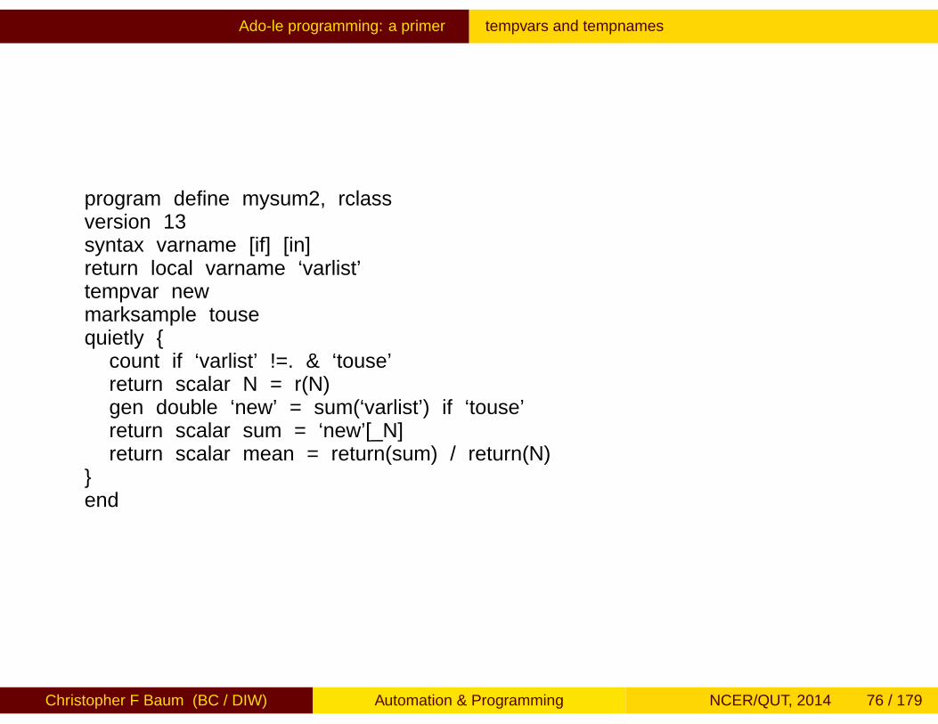
With minor modifications, this program can be enhanced to enable theif exp and in range qualifiers. We add those optional features tothe syntax command, use the marksample command to delineatethe wanted observations by touse, and apply if ‘touse’ qualifierson two computational statements:
Christopher F Baum (BC / DIW) Automation & Programming NCER/QUT, 2014 75 / 179
Ado-file programming: a primer tempvars and tempnames
program define mysum2, rclassversion 13syntax varname [if] [in]return local varname ‘varlist’tempvar newmarksample tousequietly {
count if ‘varlist’ !=. & ‘touse’return scalar N = r(N)gen double ‘new’ = sum(‘varlist’) if ‘touse’return scalar sum = ‘new’[_N]return scalar mean = return(sum) / return(N)
}end
Christopher F Baum (BC / DIW) Automation & Programming NCER/QUT, 2014 76 / 179
Examples of ado-file programming
Examples of ado-file programming
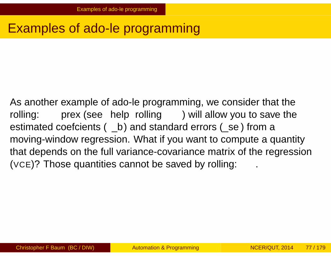
As another example of ado-file programming, we consider that therolling: prefix (see help rolling) will allow you to save theestimated coefficients (_b) and standard errors (_se) from amoving-window regression. What if you want to compute a quantitythat depends on the full variance-covariance matrix of the regression(VCE)? Those quantities cannot be saved by rolling:.
Christopher F Baum (BC / DIW) Automation & Programming NCER/QUT, 2014 77 / 179

Examples of ado-file programming
For instance, the regression
. regress y L(1/4).x
estimates the effects of the last four periods’ values of x on y. Wemight naturally be interested in the sum of the lag coefficients, as itprovides the steady-state effect of x on y. This computation is readilyperformed with lincom. If this regression is run over a movingwindow, how might we access the information needed to perform thiscomputation?
Christopher F Baum (BC / DIW) Automation & Programming NCER/QUT, 2014 78 / 179

Examples of ado-file programming
A solution is available in the form of a wrapper program which maythen be called by rolling:. We write our own r-class program,myregress, which returns the quantities of interest: the estimatedsum of lag coefficients and its standard error.
The program takes as arguments the varlist of the regression and tworequired options: lagvar(), the name of the distributed lag variable,and nlags(), the highest-order lag to be included in the lincom. Webuild up the appropriate expression for the lincom command andreturn its results to the calling program.
Christopher F Baum (BC / DIW) Automation & Programming NCER/QUT, 2014 79 / 179

Examples of ado-file programming
. type myregress.ado
*! myregress v1.0.0 CFBaum 20aug2013program myregress, rclassversion 13syntax varlist(ts) [if] [in], LAGVar(string) NLAGs(integer)regress `varlist´ `if´ `in´local nl1 = `nlags´ - 1forvalues i = 1/`nl1´ {
local lv "`lv´ L`i´.`lagvar´ + "}local lv "`lv´ L`nlags´.`lagvar´"lincom `lv´return scalar sum = `r(estimate)´return scalar se = `r(se)´end
As with any program to be used under the control of a prefix operator,it is a good idea to execute the program directly to test it to ensure thatits results are those you could calculate directly with lincom.
Christopher F Baum (BC / DIW) Automation & Programming NCER/QUT, 2014 80 / 179
Examples of ado-file programming
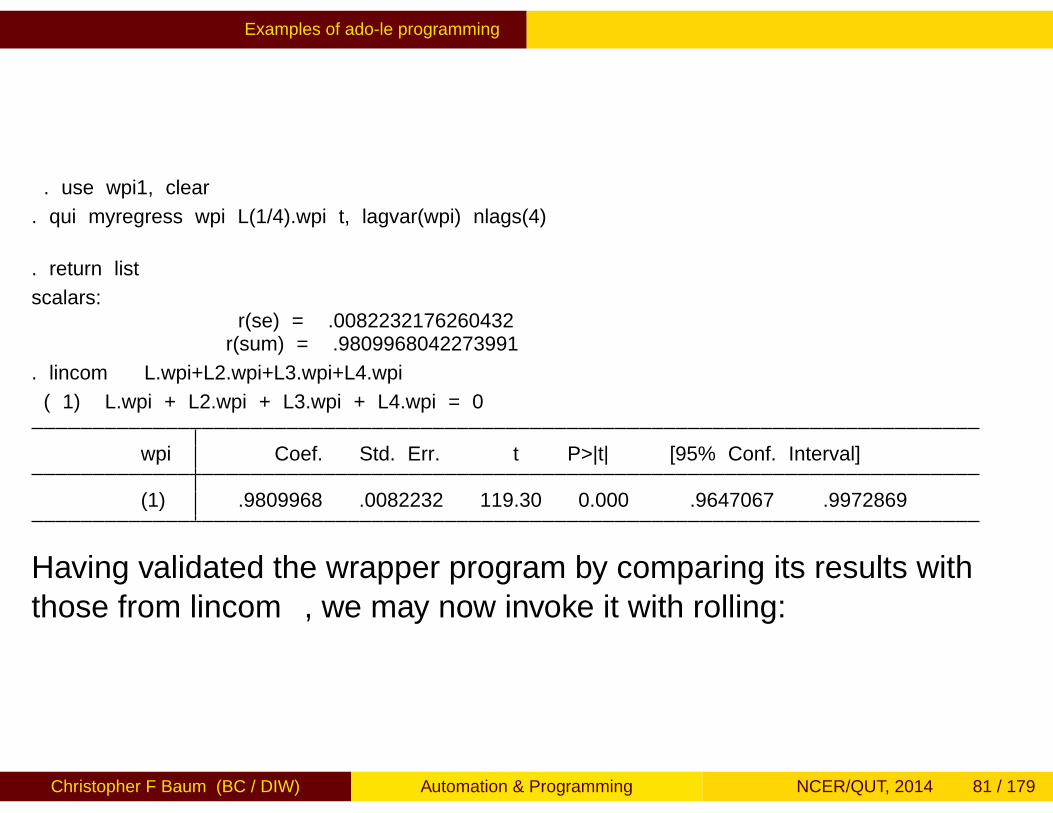
. use wpi1, clear
. qui myregress wpi L(1/4).wpi t, lagvar(wpi) nlags(4)
. return list
scalars:r(se) = .0082232176260432r(sum) = .9809968042273991
. lincom L.wpi+L2.wpi+L3.wpi+L4.wpi
( 1) L.wpi + L2.wpi + L3.wpi + L4.wpi = 0
wpi Coef. Std. Err. t P>|t| [95% Conf. Interval]
(1) .9809968 .0082232 119.30 0.000 .9647067 .9972869
Having validated the wrapper program by comparing its results withthose from lincom, we may now invoke it with rolling:
Christopher F Baum (BC / DIW) Automation & Programming NCER/QUT, 2014 81 / 179

Examples of ado-file programming
. rolling sum=r(sum) se=r(se) ,window(30) : ///> myregress wpi L(1/4).wpi t, lagvar(wpi) nlags(4)(running myregress on estimation sample)
Rolling replications (95)1 2 3 4 5
.................................................. 50
.............................................
We may graph the resulting series and its approximate 95% standarderror bands with twoway rarea and tsline:. tsset end, quarterly
time variable: end, 1967q2 to 1990q4delta: 1 quarter
. label var end Endpoint
. g lo = sum - 1.96 * se
. g hi = sum + 1.96 * se
. twoway rarea lo hi end, color(gs12) title("Sum of moving lag coefficients, ap> prox. 95% CI") ///> || tsline sum, legend(off) scheme(s2mono)
Christopher F Baum (BC / DIW) Automation & Programming NCER/QUT, 2014 82 / 179

Examples of ado-file programming
.51
1.5
2
1965q1 1970q1 1975q1 1980q1 1985q1 1990q1E ndpoint
S um of moving lag coefficients, approx. 95% C I
Christopher F Baum (BC / DIW) Automation & Programming NCER/QUT, 2014 83 / 179

Programming ml, nl, nlsur, gmm function evaluators Maximum likelihood estimation
Maximum likelihood estimation
For many limited dependent models, Stata contains commands with“canned” likelihood functions which are as easy to use as regress.However, you may have to write your own likelihood evaluation routineif you are trying to solve a non-standard maximum likelihoodestimation problem.
In Stata 13, the mlexp command allows you to specify somemaximum likelihood problems in the ‘substitutable expression’ syntax.As this approach is somewhat restrictive in its applicability, we will notdiscuss it further.
Christopher F Baum (BC / DIW) Automation & Programming NCER/QUT, 2014 84 / 179

Programming ml, nl, nlsur, gmm function evaluators Maximum likelihood estimation
A key resource for ML estimation is the book Maximum LikelihoodEstimation in Stata, Gould, Pitblado and Poi, Stata Press: 4th ed.,2010. A good deal of this presentation is adapted from their excellenttreatment of the subject, which I recommend that you buy if you aregoing to work with MLE in Stata.
To perform maximum likelihood estimation (MLE) in Stata using ml,you must write a short Stata program defining the likelihood functionfor your problem. In most cases, that program can be quite generaland may be applied to a number of different model specificationswithout the need for modifying the program.
Christopher F Baum (BC / DIW) Automation & Programming NCER/QUT, 2014 85 / 179

Programming ml, nl, nlsur, gmm function evaluators Example: binomial probit
Let’s consider the simplest use of MLE: a model that estimates abinomial probit equation, as implemented in official Stata by theprobit command. We code our probit ML program as:
program myprobit_lfversion 13args lnf xbquietly replace `lnf´ = ln(normal( `xb´ )) if $ML_y1 == 1quietly replace `lnf´ = ln(normal( -`xb´ )) if $ML_y1 == 0
end
Christopher F Baum (BC / DIW) Automation & Programming NCER/QUT, 2014 86 / 179

Programming ml, nl, nlsur, gmm function evaluators Example: binomial probit
This program is suitable for ML estimation in the linear form or lfcontext. The local macro lnf contains the contribution to log-likelihoodof each observation in the defined sample. As is generally the casewith Stata’s generate and replace, it is not necessary to loop overthe observations. In the linear form context, the program need not sumup the log-likelihood.
Christopher F Baum (BC / DIW) Automation & Programming NCER/QUT, 2014 87 / 179
Programming ml, nl, nlsur, gmm function evaluators Example: binomial probit
Several programming constructs show up in this example. The argsstatement defines the program’s arguments: lnf, the variable that willcontain the value of log-likelihood for each observation, and xb, thelinear form: a single variable that is the product of the “X matrix” andthe current vector b. The arguments are local macros within theprogram.
The program replaces the values of lnf with the appropriatelog-likelihood values, conditional on the value of $ML_y1: the firstdependent variable or “y”-variable. Thus, the program may be appliedto any 0–1 variable as a function of any set of X variables withoutmodification.
Christopher F Baum (BC / DIW) Automation & Programming NCER/QUT, 2014 88 / 179
Programming ml, nl, nlsur, gmm function evaluators Example: binomial probit
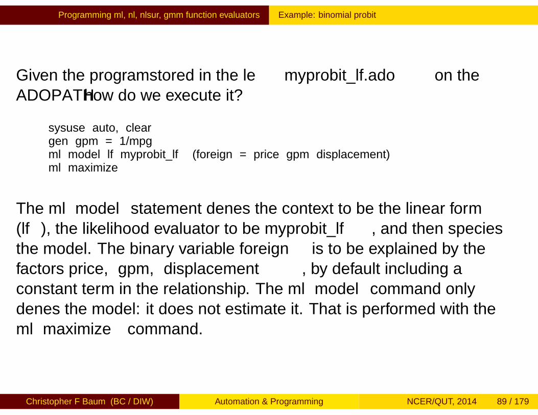
Given the program—stored in the file myprobit_lf.ado on theADOPATH—how do we execute it?
sysuse auto, cleargen gpm = 1/mpgml model lf myprobit_lf (foreign = price gpm displacement)ml maximize
The ml model statement defines the context to be the linear form(lf), the likelihood evaluator to be myprobit_lf, and then specifiesthe model. The binary variable foreign is to be explained by thefactors price, gpm, displacement, by default including aconstant term in the relationship. The ml model command onlydefines the model: it does not estimate it. That is performed with theml maximize command.
Christopher F Baum (BC / DIW) Automation & Programming NCER/QUT, 2014 89 / 179

Programming ml, nl, nlsur, gmm function evaluators Example: binomial probit
You can verify that this routine duplicates the results of applyingprobit to the same model. Note that our ML program producesestimation results in the same format as an official Stata command. Italso stores its results in the ereturn list, so that postestimationcommands such as test and lincom are available.
Of course, we need not write our own binomial probit. To understandhow we might apply Stata’s ML commands to a likelihood function ofour own, we must establish some notation, and explain what the linearform context implies.
Christopher F Baum (BC / DIW) Automation & Programming NCER/QUT, 2014 90 / 179
Programming ml, nl, nlsur, gmm function evaluators Basic notation
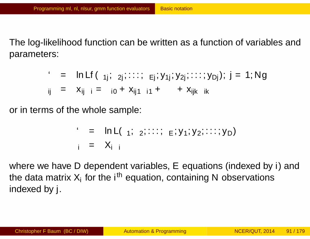
The log-likelihood function can be written as a function of variables andparameters:
` = ln L{(θ1j , θ2j , . . . , θEj ; y1j , y2j , . . . , yDj), j = 1,N}θij = xijβi = βi0 + xij1βi1 + · · ·+ xijkβik
or in terms of the whole sample:
` = ln L(θ1, θ2, . . . , θE ;y1,y2, . . . ,yD)
θi = Xiβi
where we have D dependent variables, E equations (indexed by i) andthe data matrix Xi for the i th equation, containing N observationsindexed by j .
Christopher F Baum (BC / DIW) Automation & Programming NCER/QUT, 2014 91 / 179

Programming ml, nl, nlsur, gmm function evaluators Basic notation
In the special case where the log-likelihood contribution can becalculated separately for each observation and the sum of thosecontributions is the overall log-likelihood, the model is said to meet thelinear form restrictions:
ln `j = ln `(θ1j , θ2j , . . . , θEj ; y1j , y2j , . . . , yDj)
` =N∑
j=1
ln `j
which greatly simplify the task of specifying the model. Nevertheless,when the linear form restrictions are not met, Stata provides threeother contexts in which the full likelihood function (and possibly itsderivatives) can be specified.
Christopher F Baum (BC / DIW) Automation & Programming NCER/QUT, 2014 92 / 179

Programming ml, nl, nlsur, gmm function evaluators Specifying the ML equations
One of the more difficult concepts in Stata’s MLE approach is thenotion of ML equations. In the example above, we only specified asingle equation:
(foreign = price gpm displacement)
which served to identify the dependent variable ($ML_y1 to Stata) andthe X variables in our binomial probit model.
Let’s consider how we can implement estimation of a linear regressionmodel via ML. In regression we seek to estimate not only thecoefficient vector b but the error variance σ2. The log-likelihoodfunction for the linear regression model with normally distributed errorsis:
ln L =N∑
j=1
[lnφ{(yj − xjβ)/σ} − lnσ]
with parameters β, σ to be estimated.
Christopher F Baum (BC / DIW) Automation & Programming NCER/QUT, 2014 93 / 179

Programming ml, nl, nlsur, gmm function evaluators Specifying the ML equations
Writing the conditional mean of y for the j th observation as µj ,
µj = E(yj) = xjβ
we can rewrite the log-likelihood function as
θ1j = µj = x1jβ1
θ2j = σj = x2jβ2
ln L =N∑
j=1
[lnφ{(yj − θ1j)/θ2j} − ln θ2j ]
Christopher F Baum (BC / DIW) Automation & Programming NCER/QUT, 2014 94 / 179
Programming ml, nl, nlsur, gmm function evaluators Specifying the ML equations
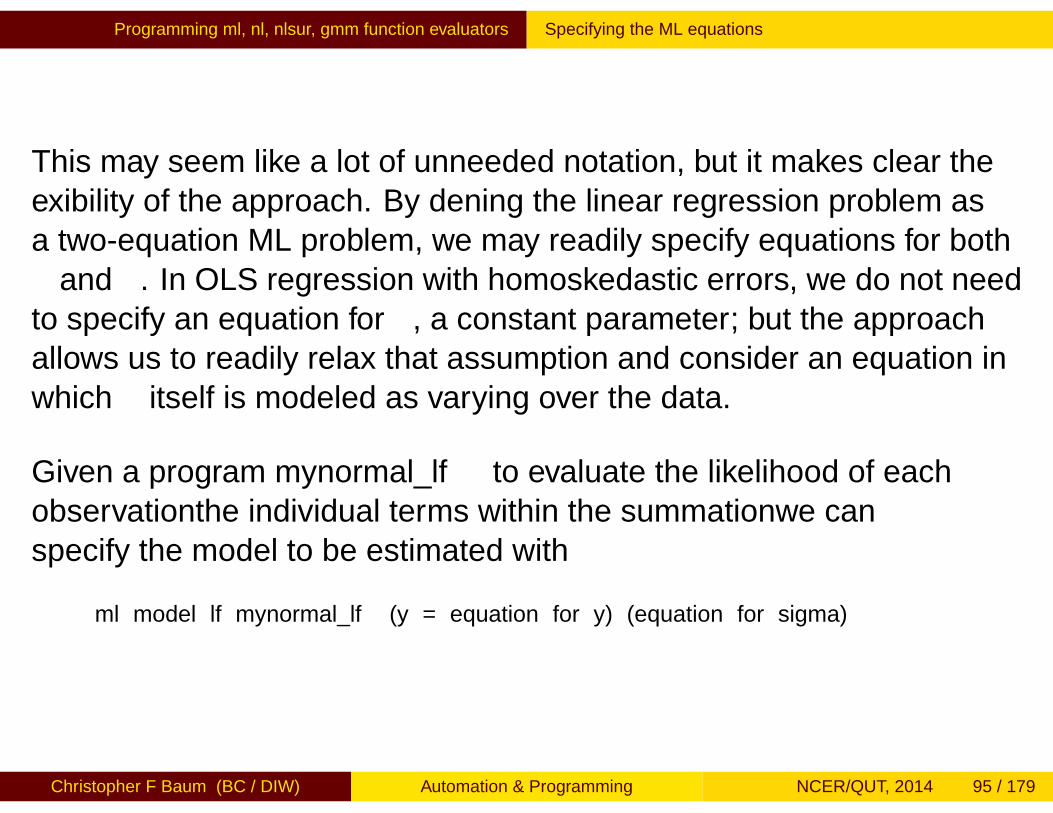
This may seem like a lot of unneeded notation, but it makes clear theflexibility of the approach. By defining the linear regression problem asa two-equation ML problem, we may readily specify equations for bothβ and σ. In OLS regression with homoskedastic errors, we do not needto specify an equation for σ, a constant parameter; but the approachallows us to readily relax that assumption and consider an equation inwhich σ itself is modeled as varying over the data.
Given a program mynormal_lf to evaluate the likelihood of eachobservation—the individual terms within the summation—we canspecify the model to be estimated with
ml model lf mynormal_lf (y = equation for y) (equation for sigma)
Christopher F Baum (BC / DIW) Automation & Programming NCER/QUT, 2014 95 / 179

Programming ml, nl, nlsur, gmm function evaluators Specifying the ML equations
In the homoskedastic linear regression case, this might look like
ml model lf mynormal_lf (mpg = weight displacement) ()
where the trailing set of () merely indicate that nothing but a constantappears in the “equation” for σ. This ml model specification indicatesthat a regression of mpg on weight and displacement is to be fit,by default with a constant term.
We could also use the notation
ml model lf mynormal_lf (mpg = weight displacement) /sigma
where there is a constant parameter to be estimated.
Christopher F Baum (BC / DIW) Automation & Programming NCER/QUT, 2014 96 / 179

Programming ml, nl, nlsur, gmm function evaluators Specifying the ML equations
But what does the program mynormal_lf contain?
program mynormal_lfversion 13args lnf mu sigmaquietly replace `lnf´ = ln(normalden( $ML_y1, `mu´, `sigma´ ))
end
We can use Stata’s normalden(x,m,s) function in this context. Thethree-parameter form of this Stata function returns the Normal[m,s]density associated with x divided by s. m, µj in the earlier notation, isthe conditional mean, computed as Xβ, while s, or σ, is the standarddeviation. By specifying an “equation” for σ of (), we indicate that asingle, constant parameter is to be estimated in that equation.
Christopher F Baum (BC / DIW) Automation & Programming NCER/QUT, 2014 97 / 179
Programming ml, nl, nlsur, gmm function evaluators Specifying the ML equations
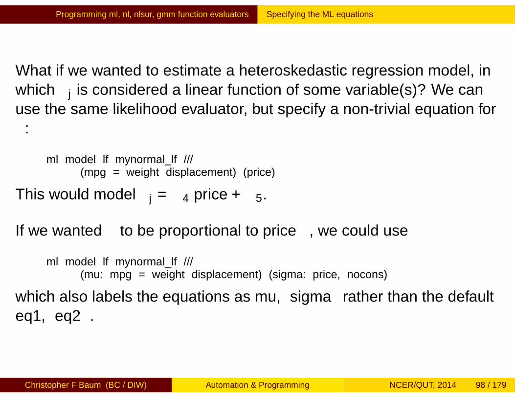
What if we wanted to estimate a heteroskedastic regression model, inwhich σj is considered a linear function of some variable(s)? We canuse the same likelihood evaluator, but specify a non-trivial equation forσ:
ml model lf mynormal_lf ///(mpg = weight displacement) (price)
This would model σj = β4 price + β5.
If we wanted σ to be proportional to price, we could use
ml model lf mynormal_lf ///(mu: mpg = weight displacement) (sigma: price, nocons)
which also labels the equations as mu, sigma rather than the defaulteq1, eq2.
Christopher F Baum (BC / DIW) Automation & Programming NCER/QUT, 2014 98 / 179

Programming ml, nl, nlsur, gmm function evaluators Specifying the ML equations
A better approach to this likelihood evaluator program involvesmodeling σ in log space, allowing it to take on all values on the realline. The likelihood evaluator program becomes
program mynormal_lf2version 13args lnf mu lnsigmaquietly replace `lnf´ = ///ln(normalden( $ML_y1, `mu´, exp(`lnsigma´ )))
end
It may be invoked by
ml model lf mynormal_lf2 ///(mpg = weight displacement) /lnsigma, ///diparm(lnsigma, exp label("sigma"))
Where the diparm( ) option presents the estimate of σ.
Christopher F Baum (BC / DIW) Automation & Programming NCER/QUT, 2014 99 / 179

Programming ml, nl, nlsur, gmm function evaluators Likelihood evaluator methods
We have illustrated the simplest likelihood evaluator method: the linearform (lf) context. It should be used whenever possible, as it is notonly easier to code (and less likely to code incorrectly) but moreaccurate. When it cannot be used—when the linear form restrictionsare not met—you may use methods d0, d1, or d2.
Method d0, like lf, requires only that you code the log-likelihoodfunction, but in its entirety rather than for a single observation. It is theleast accurate and slowest ML method, but the easiest to use whenmethod lf is not available.
Christopher F Baum (BC / DIW) Automation & Programming NCER/QUT, 2014 100 / 179

Programming ml, nl, nlsur, gmm function evaluators Likelihood evaluator methods
Method d1 requires that you code both the log-likelihood function andthe vector of first derivatives, or gradients. It is more difficult than d0,as those derivatives must be derived analytically and coded, but ismore accurate and faster than d0 (but less accurate and slower thanlf.
Method d2 requires that you code the log-likelihood function, thevector of first derivatives and the matrix of second partial derivatives. Itis the most difficult method to use, as those derivatives must bederived analytically and coded, but it is the most accurate and fastestmethod available. Unless you plan to use a ML program veryextensively, you probably do not want to go to the trouble of writing amethod d2 likelihood evaluator.
Christopher F Baum (BC / DIW) Automation & Programming NCER/QUT, 2014 101 / 179

Programming ml, nl, nlsur, gmm function evaluators Standard estimation features
Many of Stata’s standard estimation features are readily availablewhen writing ML programs.
You may estimate over a subsample with the standard if exp or inrange qualifiers on the ml model statement.
The default variance-covariance matrix (vce(oim)) estimator is basedon the inverse of the estimated Hessian, or information matrix, atconvergence. That matrix is available when using the defaultNewton–Raphson optimization method, which relies upon estimatedsecond derivatives of the log-likelihood function.
Christopher F Baum (BC / DIW) Automation & Programming NCER/QUT, 2014 102 / 179

Programming ml, nl, nlsur, gmm function evaluators Standard estimation features
If any of the quasi-Newton methods are used, you may select the OuterProduct of Gradients (vce(opg)) estimator of the variance-covariancematrix, which does not rely on a calculated Hessian. This may beespecially helpful if you have a lengthy parameter vector. You canspecify that the covariance matrix is based on the information matrix(vce(oim)) even with the quasi-Newton methods.
The standard heteroskedasticity-robust vce estimate is available byselecting the vce(robust) option (unless using method d0).Likewise, the cluster-robust covariance matrix may be selected, as instandard estimation, with cluster(varname).
Christopher F Baum (BC / DIW) Automation & Programming NCER/QUT, 2014 103 / 179
Programming ml, nl, nlsur, gmm function evaluators Standard estimation features
You may estimate a model subject to linear constraints using thestandard constraint command and the constraints( ) optionon the ml model command.
You may specify weights on the ml model command, using theweights syntax applicable to any estimation command. If you specifypweights (probability weights) robust estimates of thevariance-covariance matrix are implied.
You may use the svy option to indicate that the data have beensvyset: that is, derived from a complex survey design.
Christopher F Baum (BC / DIW) Automation & Programming NCER/QUT, 2014 104 / 179

Programming ml, nl, nlsur, gmm function evaluators ml for linear form models
A method lf likelihood evaluator program will look like:
program myprogversion 13args lnf theta1 theta2 ...tempvar tmp1 tmp2 ...qui gen double `tmp1´ = ...qui replace `lnf´ = ...
end
Christopher F Baum (BC / DIW) Automation & Programming NCER/QUT, 2014 105 / 179

Programming ml, nl, nlsur, gmm function evaluators ml for linear form models
ml places the name of each dependent variable specified in mlmodel in a global macro: $ML_y1, $ML_y2, and so on.
ml supplies a variable for each equation specified in ml model astheta1, theta2, etc. Those variables contain linear combinations ofthe explanatory variables and current coefficients of their respectiveequations. These variables must not be modified within the program.
Christopher F Baum (BC / DIW) Automation & Programming NCER/QUT, 2014 106 / 179

Programming ml, nl, nlsur, gmm function evaluators ml for linear form models
If you need to compute any intermediate results within the program,use tempvars, and declare them as double. If scalars are needed,define them with a tempname statement. Computation of componentsof the LLF is often convenient when it is a complicated expression.
Final results are saved in ‘lnf’: a double-precision variable that willcontain the contributions to likelihood of each observation.
The linear form restrictions require that the individual observations inthe dataset correspond to independent pieces of the log-likelihoodfunction. They will be met for many ML problems, but are violated forproblems involving panel data, fixed-effect logit models, and Coxregression.
Christopher F Baum (BC / DIW) Automation & Programming NCER/QUT, 2014 107 / 179

Programming ml, nl, nlsur, gmm function evaluators ml for linear form models
Just as linear regression may be applied to many nonlinear models(e.g., the Cobb–Douglas production function), Stata’s linear formrestrictions do not hinder our estimation of a nonlinear model. Wemerely add equations to define components of the model. If we wantto estimate
yj = β1x1j + β2x2j + β3xβ43j + β5 + εj
with ε ∼ N(0, σ2), we can express the log-likelihood as
ln `j = lnφ{(yj − θ1j − θ2jxθ3j3j )/θ4j} − ln θ4j
θ1j = β1x1j + β2x2j + β5
θ2j = β3
θ3j = β4
θ4j = σ
Christopher F Baum (BC / DIW) Automation & Programming NCER/QUT, 2014 108 / 179
Programming ml, nl, nlsur, gmm function evaluators ml for linear form models
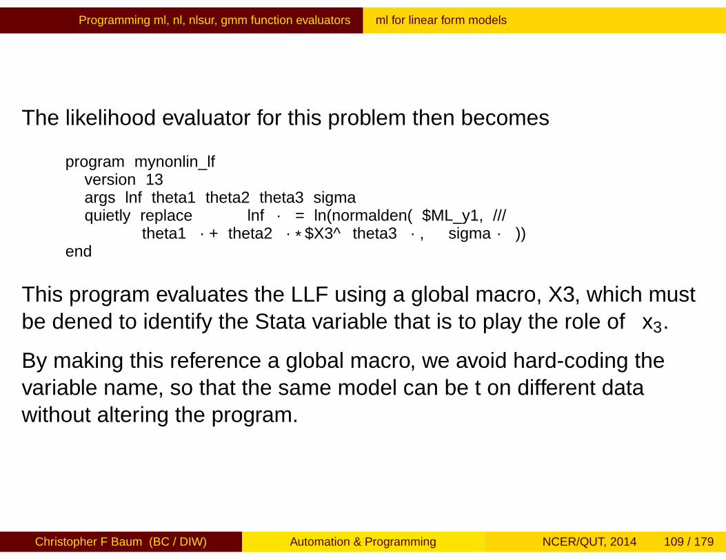
The likelihood evaluator for this problem then becomes
program mynonlin_lfversion 13args lnf theta1 theta2 theta3 sigmaquietly replace `lnf´ = ln(normalden( $ML_y1, ///
`theta1´+`theta2´*$X3^`theta3´, `sigma´ ))end
This program evaluates the LLF using a global macro, X3, which mustbe defined to identify the Stata variable that is to play the role of x3.
By making this reference a global macro, we avoid hard-coding thevariable name, so that the same model can be fit on different datawithout altering the program.
Christopher F Baum (BC / DIW) Automation & Programming NCER/QUT, 2014 109 / 179

Programming ml, nl, nlsur, gmm function evaluators ml for linear form models
We could invoke the program with
global X3 bp0ml model lf mynonlin_lf (bp = age sex) /beta3 /beta4 /sigmaml maximize
Thus, we may readily handle a nonlinear regression model in thiscontext of the linear form restrictions, redefining the ML problem asone of four equations.
If we need to set starting values, we can do so with the ml initcommand. The ml check command is very useful in testing thelikelihood evaluator program and ensuring that it is working properly.The ml search command is recommended to find appropriatestarting values. The ml query command can be used to evaluate theprogress of ML if there are difficulties achieving convergence.
Christopher F Baum (BC / DIW) Automation & Programming NCER/QUT, 2014 110 / 179
Programming ml, nl, nlsur, gmm function evaluators Nonlinear least squares estimators
Nonlinear least squares estimation
Besides the capabilities for maximum likelihood estimation of one orseveral equations via the ml suite of commands, Stata providesfacilities for single-equation nonlinear least squares estimation with nland the estimation of nonlinear systems of equations with nlsur.
In an earlier session, we discussed interactive use of thesecommands. We now describe how they may be used with a functionevaluator program, which is quite similar to the likelihood functionevaluators for ml that we just discussed.
Christopher F Baum (BC / DIW) Automation & Programming NCER/QUT, 2014 111 / 179

Programming ml, nl, nlsur, gmm function evaluators nl function evaluator program
If you want to use nl extensively for a particular problem, it makessense to develop a function evaluator program. That program is quitesimilar to any Stata ado-file or ml program. It must be namednlfunc.ado, where func is a name of your choice: e.g., nlces.adofor a CES function evaluator.
The stylized function evaluator program contains:
program nlfuncversion 13syntax varlist(min=n max=n) if, at(name)
// extract vars from varlist// extract params as scalars from at matrix// fill in dependent variable with replaceend
Christopher F Baum (BC / DIW) Automation & Programming NCER/QUT, 2014 112 / 179
Programming ml, nl, nlsur, gmm function evaluators nl function evaluator program
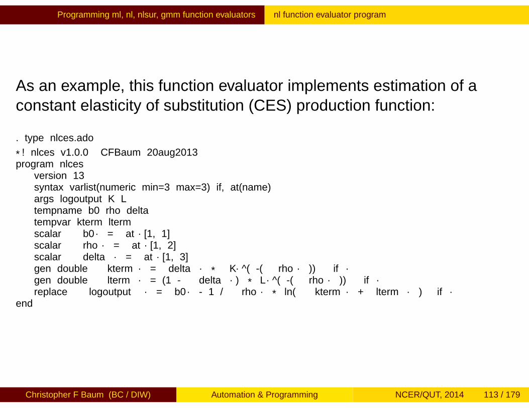
As an example, this function evaluator implements estimation of aconstant elasticity of substitution (CES) production function:
. type nlces.ado
*! nlces v1.0.0 CFBaum 20aug2013program nlces
version 13syntax varlist(numeric min=3 max=3) if, at(name)args logoutput K Ltempname b0 rho deltatempvar kterm ltermscalar `b0´ = `at´[1, 1]scalar `rho´ = `at´[1, 2]scalar `delta´ = `at´[1, 3]gen double `kterm´ = `delta´ * `K´^( -(`rho´ )) `if´gen double `lterm´ = (1 - `delta´) *`L´^( -(`rho´ )) `if´replace `logoutput´ = `b0´ - 1 / `rho´ * ln( `kterm´ + `lterm´ ) `if´
end
Christopher F Baum (BC / DIW) Automation & Programming NCER/QUT, 2014 113 / 179
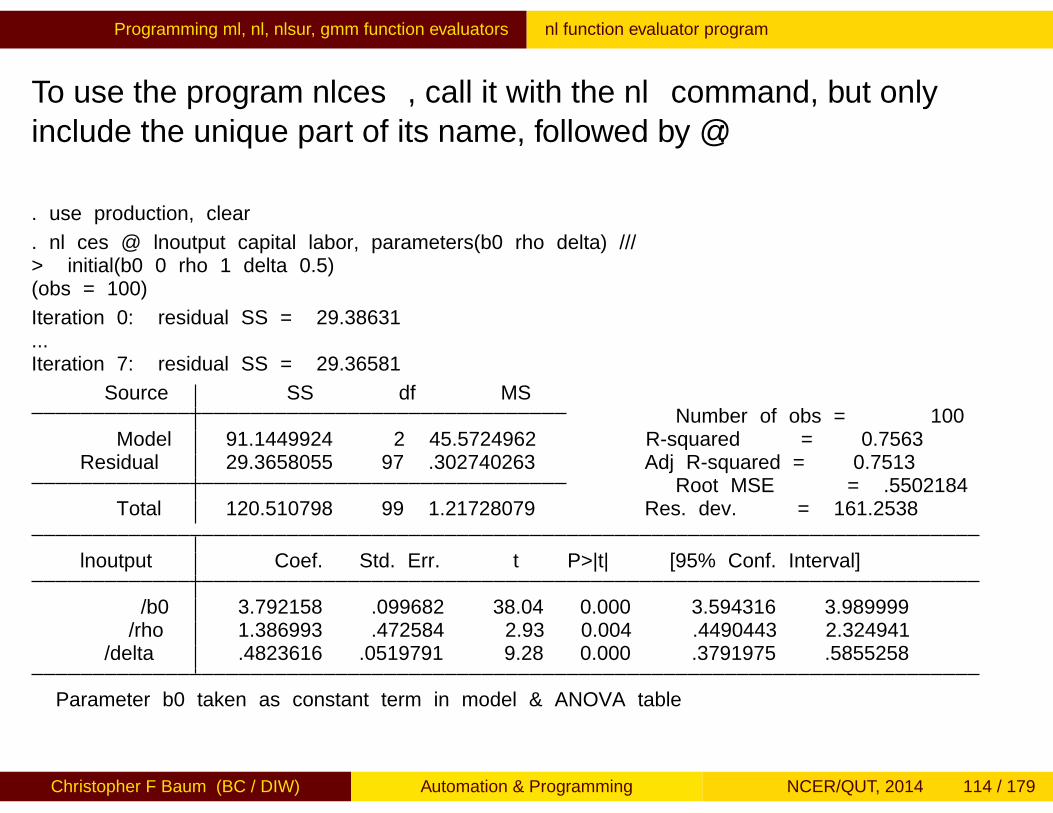
Programming ml, nl, nlsur, gmm function evaluators nl function evaluator program
To use the program nlces, call it with the nl command, but onlyinclude the unique part of its name, followed by @:
. use production, clear
. nl ces @ lnoutput capital labor, parameters(b0 rho delta) ///> initial(b0 0 rho 1 delta 0.5)(obs = 100)
Iteration 0: residual SS = 29.38631...Iteration 7: residual SS = 29.36581
Source SS df MSNumber of obs = 100
Model 91.1449924 2 45.5724962 R-squared = 0.7563Residual 29.3658055 97 .302740263 Adj R-squared = 0.7513
Root MSE = .5502184Total 120.510798 99 1.21728079 Res. dev. = 161.2538
lnoutput Coef. Std. Err. t P>|t| [95% Conf. Interval]
/b0 3.792158 .099682 38.04 0.000 3.594316 3.989999/rho 1.386993 .472584 2.93 0.004 .4490443 2.324941
/delta .4823616 .0519791 9.28 0.000 .3791975 .5855258
Parameter b0 taken as constant term in model & ANOVA table
Christopher F Baum (BC / DIW) Automation & Programming NCER/QUT, 2014 114 / 179

Programming ml, nl, nlsur, gmm function evaluators nl function evaluator program
You could restrict analysis to a subsample with the if exp qualifier:
nl ces @ lnQ cap lab if industry==33, ...
You can also perform post-estimation commands, such as nlcom, toderive point and interval estimates of nonlinear combinations of theestimated parameters. In this case, we want to compute the elasticityof substitution, σ:
. nlcom (sigma: 1 / ( 1 + [rho]_b[_cons] ))
sigma: 1 / ( 1 + [rho]_b[_cons] )
lnoutput Coef. Std. Err. t P>|t| [95% Conf. Interval]
sigma .4189372 .0829424 5.05 0.000 .2543194 .583555
Christopher F Baum (BC / DIW) Automation & Programming NCER/QUT, 2014 115 / 179

Programming ml, nl, nlsur, gmm function evaluators nl function evaluator program
Note that the nlsur command estimates systems of seeminglyunrelated nonlinear equations, just as sureg estimates systems ofseemingly unrelated linear equations. In that context, nlsur cannotbe used to estimate a system of simultaneous nonlinear equations.The gmm command, as we now discuss, could be used for thatpurpose, as could Stata’s maximum likelihood commands (ml).
Christopher F Baum (BC / DIW) Automation & Programming NCER/QUT, 2014 116 / 179

Programming ml, nl, nlsur, gmm function evaluators GMM function-evaluator programs
GMM function-evaluator programs
The GMM function evaluator program, or moment-evaluator program,is passed a varlist containing the moments to be evaluated for eachobservation. Your program replaces the elements of the varlist with the‘error part’ of the moment conditions. For instance, if we were to solvean OLS regression problem with GMM we might write amoment-evaluator program as:
Christopher F Baum (BC / DIW) Automation & Programming NCER/QUT, 2014 117 / 179

Programming ml, nl, nlsur, gmm function evaluators GMM function-evaluator programs
. program gmm_reg1. version 132. syntax varlist if, at(name)3. qui {4. tempvar xb5. gen double `xb´ = x1*`at´[1,1] + x2*`at´[1,2] + ///
> x3*`at´[1,3] + `at´[1,4] `if´6. replace `varlist´ = y - `xb´ `if´7. }8. end
where we have specified that the regression has three explanatoryvariables and a constant term, with variable y as the dependentvariable. The row vector at() contains the current values of theestimated parameters. The contents of varlist are replaced with thediscrepancies, y − Xβ, defined by those parameters. A varlist is usedas gmm can handle multiple-equation problems.
Christopher F Baum (BC / DIW) Automation & Programming NCER/QUT, 2014 118 / 179
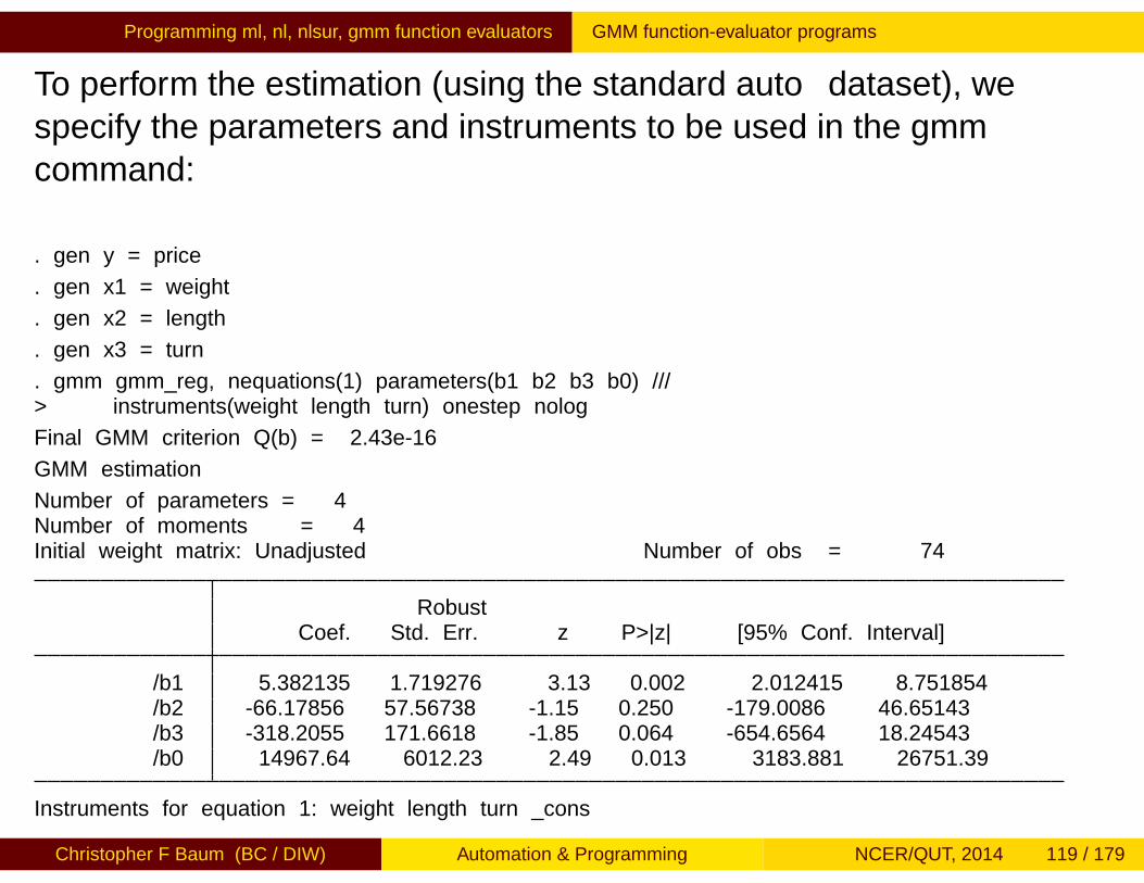
Programming ml, nl, nlsur, gmm function evaluators GMM function-evaluator programs
To perform the estimation (using the standard auto dataset), wespecify the parameters and instruments to be used in the gmmcommand:
. gen y = price
. gen x1 = weight
. gen x2 = length
. gen x3 = turn
. gmm gmm_reg, nequations(1) parameters(b1 b2 b3 b0) ///> instruments(weight length turn) onestep nolog
Final GMM criterion Q(b) = 2.43e-16
GMM estimation
Number of parameters = 4Number of moments = 4Initial weight matrix: Unadjusted Number of obs = 74
RobustCoef. Std. Err. z P>|z| [95% Conf. Interval]
/b1 5.382135 1.719276 3.13 0.002 2.012415 8.751854/b2 -66.17856 57.56738 -1.15 0.250 -179.0086 46.65143/b3 -318.2055 171.6618 -1.85 0.064 -654.6564 18.24543/b0 14967.64 6012.23 2.49 0.013 3183.881 26751.39
Instruments for equation 1: weight length turn _cons
Christopher F Baum (BC / DIW) Automation & Programming NCER/QUT, 2014 119 / 179

Programming ml, nl, nlsur, gmm function evaluators GMM function-evaluator programs
This may seem unusual syntax, but we are just stating that we want touse the regressors as instruments for themselves in solving the GMMproblem, as under the hypothesis of E [u|X ] = 0, the appropriatemoment conditions can be written as EX ′u = 0.
Inspection of the parameters and their standard errors shows thatthese estimates match those from regress, robust for the samemodel. It is quite unnecessary to use GMM in this context, of course,but it illustrates the way in which you may set up a GMM problem.
Christopher F Baum (BC / DIW) Automation & Programming NCER/QUT, 2014 120 / 179

Programming ml, nl, nlsur, gmm function evaluators GMM function-evaluator programs
To perform linear instrumental variables, we can use the samemoment-evaluator program and merely alter the instrument list:
. webuse hsng2, clear(1980 Census housing data)
. gen y = rent
. gen x1 = hsngval
. gen x2 = pcturban
. gen x3 = popden
. gmm gmm_reg, nequations(1) parameters(b1 b2 b3 b0) ///> instruments(pcturban popden faminc reg2-reg4) onestep nolog
Final GMM criterion Q(b) = 150.8821
GMM estimation
Number of parameters = 4Number of moments = 7Initial weight matrix: Unadjusted Number of obs = 50
RobustCoef. Std. Err. z P>|z| [95% Conf. Interval]
/b1 .0022538 .0006785 3.32 0.001 .000924 .0035836/b2 .0281637 .5017214 0.06 0.955 -.9551922 1.01152/b3 .0006083 .0012742 0.48 0.633 -.0018891 .0031057/b0 122.6632 17.26189 7.11 0.000 88.83052 156.4959
Instruments for equation 1: pcturban popden faminc reg2 reg3 reg4 _cons
Christopher F Baum (BC / DIW) Automation & Programming NCER/QUT, 2014 121 / 179

Programming ml, nl, nlsur, gmm function evaluators GMM function-evaluator programs
These estimates match those produced by ivregress 2sls,robust.
Let us consider solving a nonlinear estimation problem: a binomialprobit model, using GMM rather than the usual ML estimator. Themoment-evaluator program:
. program gmm_probit1. version 132. syntax varlist if, at(name)3. qui {4. tempvar xb5. gen double `xb´ = x1*`at´[1,1] + x2*`at´[1,2] + ///
> x3*`at´[1,3] + `at´[1,4] `if´6. replace `varlist´ = y - normal(`xb´)7. }8. end
Christopher F Baum (BC / DIW) Automation & Programming NCER/QUT, 2014 122 / 179

Programming ml, nl, nlsur, gmm function evaluators GMM function-evaluator programs
To perform the estimation, we specify the parameters and instrumentsto be used in the gmm command:
. webuse hsng2, clear(1980 Census housing data)
. gen y = (region >= 3)
. gen x1 = hsngval
. gen x2 = pcturban
. gen x3 = popden
. gmm gmm_probit, nequations(1) parameters(b1 b2 b3 b0) ///> instruments(pcturban hsngval popden) onestep nolog
Final GMM criterion Q(b) = 3.18e-21
GMM estimation
Number of parameters = 4Number of moments = 4Initial weight matrix: Unadjusted Number of obs = 50
RobustCoef. Std. Err. z P>|z| [95% Conf. Interval]
/b1 .0000198 .0000146 1.35 0.177 -8.92e-06 .0000484/b2 .0139055 .0177526 0.78 0.433 -.020889 .0487001/b3 -.0003561 .0001142 -3.12 0.002 -.0005799 -.0001323/b0 -1.136154 .9463889 -1.20 0.230 -2.991042 .7187345
Instruments for equation 1: pcturban hsngval popden _cons
Christopher F Baum (BC / DIW) Automation & Programming NCER/QUT, 2014 123 / 179

Programming ml, nl, nlsur, gmm function evaluators GMM function-evaluator programs
Inspection of the parameters shows that these estimates are quitesimilar to those from probit for the same model. However, whereasprobit requires the assumption of i .i .d . errors, GMM does not; thestandard errors produced by gmm are robust to arbitraryheteroskedasticity.
As in the case of our linear regression estimation example, we can usethe same moment-evaluator program to estimate aninstrumental-variables probit model, similar to that estimated byivprobit. Unlike that ML command, though, we need not make anydistributional assumptions about the error process in order to useGMM.
Christopher F Baum (BC / DIW) Automation & Programming NCER/QUT, 2014 124 / 179
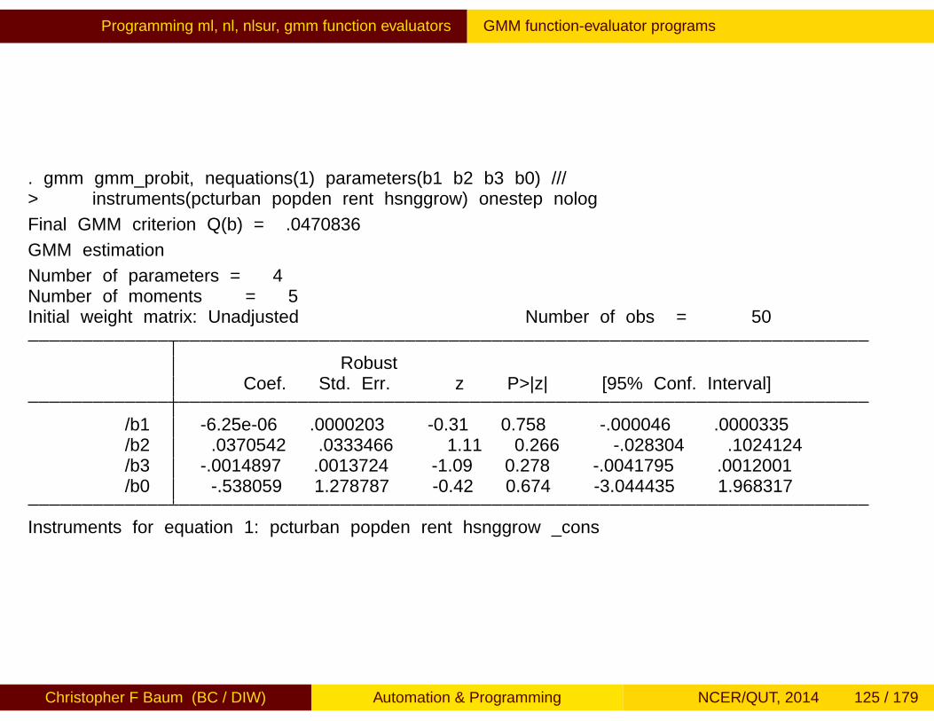
Programming ml, nl, nlsur, gmm function evaluators GMM function-evaluator programs
. gmm gmm_probit, nequations(1) parameters(b1 b2 b3 b0) ///> instruments(pcturban popden rent hsnggrow) onestep nolog
Final GMM criterion Q(b) = .0470836
GMM estimation
Number of parameters = 4Number of moments = 5Initial weight matrix: Unadjusted Number of obs = 50
RobustCoef. Std. Err. z P>|z| [95% Conf. Interval]
/b1 -6.25e-06 .0000203 -0.31 0.758 -.000046 .0000335/b2 .0370542 .0333466 1.11 0.266 -.028304 .1024124/b3 -.0014897 .0013724 -1.09 0.278 -.0041795 .0012001/b0 -.538059 1.278787 -0.42 0.674 -3.044435 1.968317
Instruments for equation 1: pcturban popden rent hsnggrow _cons
Christopher F Baum (BC / DIW) Automation & Programming NCER/QUT, 2014 125 / 179

Programming ml, nl, nlsur, gmm function evaluators GMM function-evaluator programs
Although the examples of gmm moment-evaluator programs we haveshown here largely duplicate the functionality of existing Statacommands, they should illustrate that the general-purpose gmmcommand may be used to solve estimation problems not amenable toany existing commands, or indeed to a maximum-likelihood approach.In that sense, familiarity with gmm capabilities is likely to be quitehelpful if you face challenging estimation problems in your research.
Christopher F Baum (BC / DIW) Automation & Programming NCER/QUT, 2014 126 / 179
Programming ml, nl, nlsur, gmm function evaluators egen functions
egen functions
The egen (Extended Generate) command is open-ended, in that anyStata user may define an additional egen function by writing aspecialized ado-file program.The name of the program (and of the filein which it resides) must start with _g: that is, _gcrunch.ado willdefine the crunch() function for egen.
Christopher F Baum (BC / DIW) Automation & Programming NCER/QUT, 2014 127 / 179

Programming ml, nl, nlsur, gmm function evaluators egen functions
To illustrate egen functions, let us create a function to generate the90–10 percentile range of a variable. The syntax for egen is:
egen[type
]newvar = fcn(arguments)
[if][
in] [
, options]
The egen command, like generate, may specify a data type. Thesyntax command indicates that a newvarname must be provided,followed by an equals sign and an fcn, or function, with arguments.egen functions may also handle if exp and in range qualifiers andoptions.
Christopher F Baum (BC / DIW) Automation & Programming NCER/QUT, 2014 128 / 179
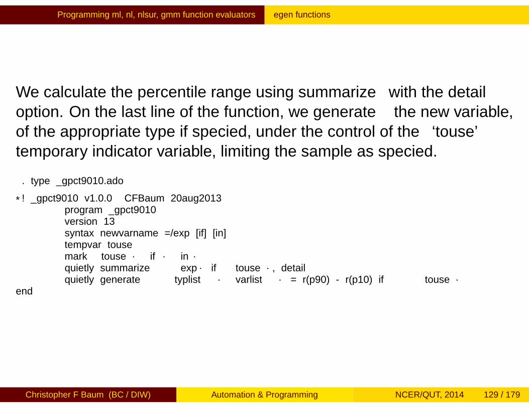
Programming ml, nl, nlsur, gmm function evaluators egen functions
We calculate the percentile range using summarize with the detailoption. On the last line of the function, we generate the new variable,of the appropriate type if specified, under the control of the ‘touse’temporary indicator variable, limiting the sample as specified.
. type _gpct9010.ado
*! _gpct9010 v1.0.0 CFBaum 20aug2013program _gpct9010version 13syntax newvarname =/exp [if] [in]tempvar tousemark `touse´ `if´ `in´quietly summarize `exp´ if `touse´, detailquietly generate `typlist´ `varlist´ = r(p90) - r(p10) if `touse´
end
Christopher F Baum (BC / DIW) Automation & Programming NCER/QUT, 2014 129 / 179

Programming ml, nl, nlsur, gmm function evaluators egen functions
This function works perfectly well, but it creates a new variablecontaining a single scalar value. As noted earlier, that is a veryprofligate use of Stata’s memory (especially for large _N) and oftencan be avoided by retrieving the single scalar which is convenientlystored by our pctrange command. To be useful, we would like theegen function to be byable, so that it could compute the appropriatepercentile range statistics for a number of groups defined in the data.
The changes to the code are relatively minor. We add an optionsclause to the syntax statement, as egen will pass the by prefixvariables as a by option to our program. Rather than usingsummarize, we use egen’s own pctile() function, which isdocumented as allowing the by prefix, and pass the options to thisfunction. The revised function reads:
Christopher F Baum (BC / DIW) Automation & Programming NCER/QUT, 2014 130 / 179
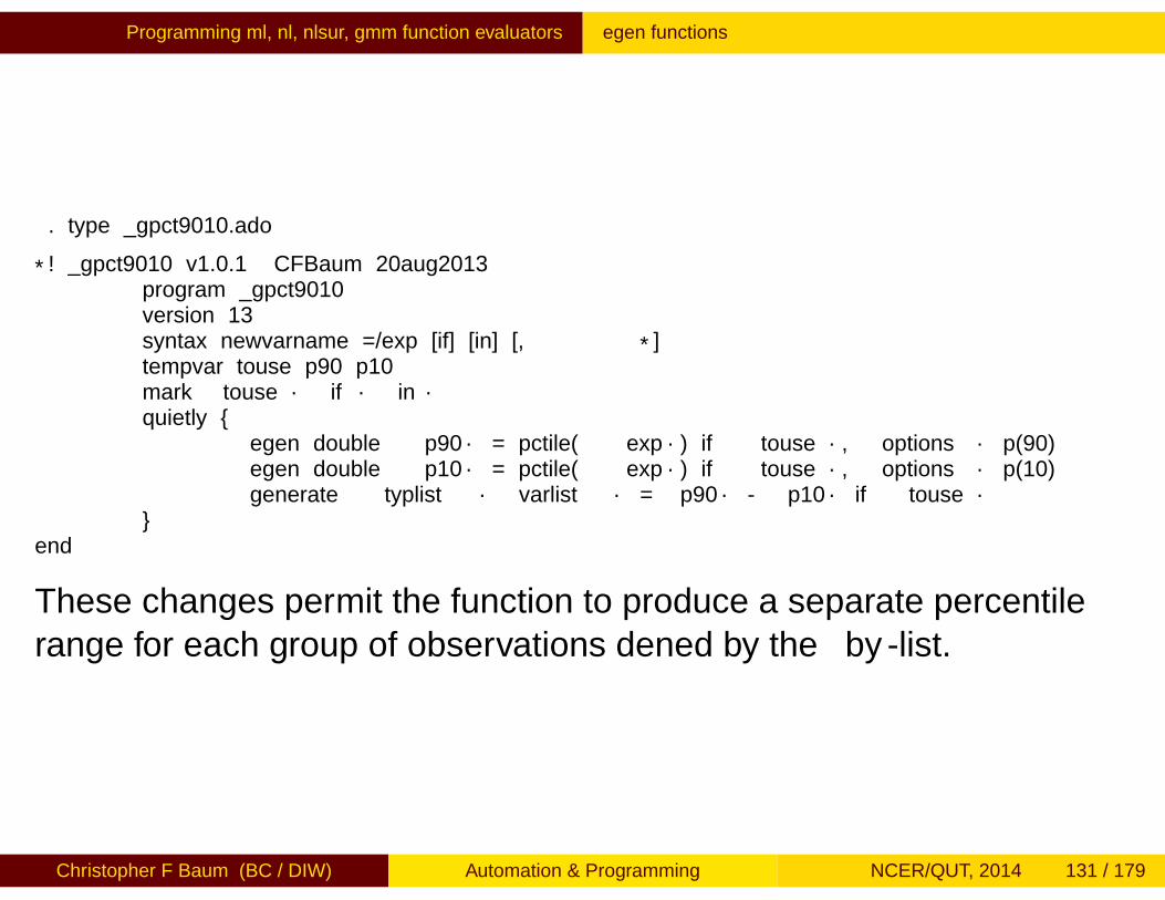
Programming ml, nl, nlsur, gmm function evaluators egen functions
. type _gpct9010.ado
*! _gpct9010 v1.0.1 CFBaum 20aug2013program _gpct9010version 13syntax newvarname =/exp [if] [in] [, *]tempvar touse p90 p10mark `touse´ `if´ `in´quietly {
egen double `p90´ = pctile(`exp´) if `touse´, `options´ p(90)egen double `p10´ = pctile(`exp´) if `touse´, `options´ p(10)generate `typlist´ `varlist´ = `p90´ - `p10´ if `touse´
}end
These changes permit the function to produce a separate percentilerange for each group of observations defined by the by-list.
Christopher F Baum (BC / DIW) Automation & Programming NCER/QUT, 2014 131 / 179

Programming ml, nl, nlsur, gmm function evaluators egen functions
To illustrate, we use auto.dta:
. sysuse auto, clear(1978 Automobile Data)
. bysort rep78 foreign: egen pctrange = pct9010(price)
Now, if we want to compute a summary statistic (such as the percentilerange) for each observation classified in a particular subset of thesample, we may use the pct9010() function to do so.
Christopher F Baum (BC / DIW) Automation & Programming NCER/QUT, 2014 132 / 179

Introduction to Mata
Introduction to Mata
We now turn to the third way in which you may use Stata programmingtechniques: by taking advantage of Mata.
Since the release of version 9, Stata has contained a full-fledgedmatrix programming language, Mata, with most of the capabilities ofMATLAB, R, Ox or Gauss. You can use Mata interactively, or you candevelop Mata functions to be called from Stata. In this talk, weemphasize the latter use of Mata.
Christopher F Baum (BC / DIW) Automation & Programming NCER/QUT, 2014 133 / 179

Introduction to Mata
Mata functions may be particularly useful where the algorithm you wishto implement already exists in matrix-language form. It is quitestraightforward to translate the logic of other matrix languages intoMata: much more so than converting it into Stata’s matrix language.
A large library of mathematical and matrix functions is provided inMata, including optimization routines, equation solvers,decompositions, eigensystem routines and probability densityfunctions. Mata functions can access Stata’s variables and can workwith virtual matrices (views) of a subset of the data in memory. Mataalso supports file input/output.
Christopher F Baum (BC / DIW) Automation & Programming NCER/QUT, 2014 134 / 179
Introduction to Mata Circumventing the limits of Stata’s matrix language
Circumventing the limits of Stata’s matrixlanguage
Mata circumvents the limitations of Stata’s traditional matrixcommands. Stata matrices must obey the maximum matsize: 800 rowsor columns in Stata/IC. Thus, code relying on Stata matrices is fragile.Stata’s matrix language does contain commands such as matrixaccum which can build a cross-product matrix from variables of anylength, but for many applications the limitation of matsize is binding.
Even in Stata/SE or Stata/MP, with the possibility of a much largermatsize, Stata’s matrices have another drawback. Large matricesconsume large amounts of memory, and an operation that convertsStata variables into a matrix or vice versa will require at least twice thememory needed for that set of variables.
Christopher F Baum (BC / DIW) Automation & Programming NCER/QUT, 2014 135 / 179

Introduction to Mata Circumventing the limits of Stata’s matrix language
The Mata programming language can sidestep these memory issuesby creating matrices with contents that refer directly to Statavariables—no matter how many variables and observations may bereferenced. These virtual matrices, or views, have minimal overhead interms of memory consumption, regardless of their size.
Unlike some matrix programming languages, Mata matrices cancontain either numeric elements or string elements (but not both). Thisimplies that you can use Mata productively in a list processingenvironment as well as in a numeric context.
For example, a prominent list-handling command, Bill Gould’sadoupdate, is written almost entirely in Mata. viewsourceadoupdate.ado reveals that only 22 lines of code (out of 1,193 lines)are in the ado-file language. The rest is Mata.
Christopher F Baum (BC / DIW) Automation & Programming NCER/QUT, 2014 136 / 179
Introduction to Mata Speed advantages
Speed advantages
Last but by no means least, ado-file code written in the matrixlanguage with explicit subscript references is slow. Even if such aroutine avoids explicit subscripting, its performance may beunacceptable. For instance, David Roodman’s xtabond2 can run inversion 7 or 8 without Mata, or in version 9 onwards with Mata. Thenon-Mata version is an order of magnitude slower when applied toreasonably sized estimation problems.
In contrast, Mata code is automatically compiled into bytecode, likeJava, and can be stored in object form or included in-line in a Statado-file or ado-file. Mata code runs many times faster than theinterpreted ado-file language, providing significant speedenhancements to many computationally burdensome tasks.
Christopher F Baum (BC / DIW) Automation & Programming NCER/QUT, 2014 137 / 179
Introduction to Mata An efficient division of labor
An efficient division of labor
Mata interfaced with Stata provides for an efficient division of labor. Ina pure matrix programming language, you must handle all of thehousekeeping details involved with data organization, transformationand selection.
In contrast, if you write an ado-file that calls one or more Matafunctions, the ado-file will handle those housekeeping details with theconvenience features of the syntax and marksample statements ofthe regular ado-file language. When the housekeeping chores arecompleted, the resulting variables can be passed on to Mata forprocessing. Results produced by Mata may then be accessed by Stataand formatted with commands like estimates display.
Christopher F Baum (BC / DIW) Automation & Programming NCER/QUT, 2014 138 / 179

Introduction to Mata An efficient division of labor
Mata can access Stata variables, local and global macros, scalars andmatrices, and modify the contents of those objects as needed. IfMata’s view matrices are used, alterations to the matrix within Matamodifies the Stata variables that comprise the view.
Christopher F Baum (BC / DIW) Automation & Programming NCER/QUT, 2014 139 / 179

Mata language elements Operators
Language syntax: Operators
To understand Mata syntax, you must be familiar with its operators.The comma is the column-join operator, so
: r1 = ( 1, 2, 3 )
creates a three-element row vector. We could also construct thisvector using the row range operator (..) as
: r1 = (1..3)
The backslash is the row-join operator, so
c1 = ( 4 5 6 )
creates a three-element column vector. We could also construct thisvector using the column range operator (::) as
: c1 = (4::6)
Christopher F Baum (BC / DIW) Automation & Programming NCER/QUT, 2014 140 / 179

Mata language elements Operators
We may combine the column-join and row-join operators:
m1 = ( 1, 2, 3 \ 4, 5, 6 \ 7, 8, 9 )
creates a 3× 3 matrix.
The matrix could also be constructed with the row range operator:
m1 = ( 1..3 \ 4..6 \ 7..9 )
Christopher F Baum (BC / DIW) Automation & Programming NCER/QUT, 2014 141 / 179

Mata language elements Operators
The prime (or apostrophe) is the transpose operator, so
r2 = ( 1 \ 2 \ 3 )´
is a row vector.
The comma and backslash operators can be used on vectors andmatrices as well as scalars, so
r3 = r1, c1´
will produce a six-element row vector, and
c2 = r1´ \ c1
creates a six-element column vector.
Matrix elements can be real or complex, so 2 - 3 i refers to acomplex number 2− 3×
√−1.
Christopher F Baum (BC / DIW) Automation & Programming NCER/QUT, 2014 142 / 179

Mata language elements Operators
The standard algebraic operators plus (+), minus (−) and multiply (∗)work on scalars or matrices:
g = r1´ + c1h = r1 * c1j = c1 * r1
In this example h will be the 1× 1 dot product of vectors r1, c1 whilej is their 3× 3 outer product.
Christopher F Baum (BC / DIW) Automation & Programming NCER/QUT, 2014 143 / 179

Mata language elements Element-wise calculations and the colon operator
Element-wise calculations and the colon operator
One of Mata’s most powerful features is the colon operator. Mata’salgebraic operators, including the forward slash (/) for division, alsocan be used in element-by-element computations when preceded by acolon:
k = r1´ :* c1
will produce a three-element column vector, with elements as theproduct of the respective elements: ki = r1i c1i , i = 1, . . . ,3.
Christopher F Baum (BC / DIW) Automation & Programming NCER/QUT, 2014 144 / 179
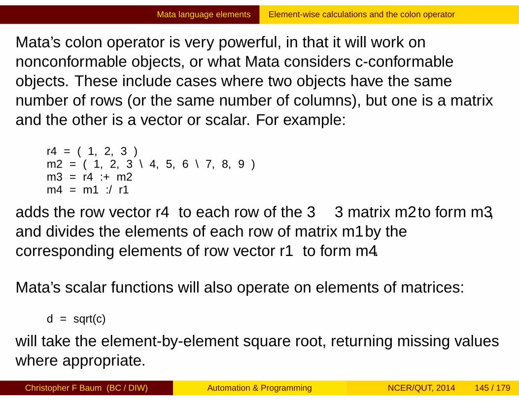
Mata language elements Element-wise calculations and the colon operator
Mata’s colon operator is very powerful, in that it will work onnonconformable objects, or what Mata considers c-conformableobjects. These include cases where two objects have the samenumber of rows (or the same number of columns), but one is a matrixand the other is a vector or scalar. For example:
r4 = ( 1, 2, 3 )m2 = ( 1, 2, 3 \ 4, 5, 6 \ 7, 8, 9 )m3 = r4 :+ m2m4 = m1 :/ r1
adds the row vector r4 to each row of the 3× 3 matrix m2 to form m3,and divides the elements of each row of matrix m1 by thecorresponding elements of row vector r1 to form m4.
Mata’s scalar functions will also operate on elements of matrices:
d = sqrt(c)
will take the element-by-element square root, returning missing valueswhere appropriate.
Christopher F Baum (BC / DIW) Automation & Programming NCER/QUT, 2014 145 / 179

Mata language elements Logical operators
Logical operators
As in Stata, the equality logical operators are a == b and a != b.They will work whether or not a and b are conformable or even of thesame type: a could be a vector and b a matrix. They return 0 or 1.
Unary not ! returns 1 if a scalar equals zero, 0 otherwise, and may beapplied in a vector or matrix context, returning a vector or matrixof 0, 1.
The remaining logical comparison operators (>, >=, <, <=) canonly be used on objects that are conformable and of the same generaltype (numeric or string). They return 0 or 1.
As in Stata, the logical and (&) and or (|) operators may only beapplied to real scalars.
Christopher F Baum (BC / DIW) Automation & Programming NCER/QUT, 2014 146 / 179

Mata language elements Subscripting
Subscripting
Subscripts in Mata utilize square brackets, and may appear on eitherthe left or right of an algebraic expression. There are two forms: listsubscripts and range subscripts.
With list subscripts, you can reference a single element of an array asx[i,j]. But i or j can also be a vector: x[i,jvec], where jvec=(4,6,8) references row i and those three columns of x. Missingvalues (dots) reference all rows or columns, so x[i,.] or x[i,]extracts row i, and x[.,.] or x[,] references the whole matrix.
You may also use range operators to avoid listing each consecutiveelement: x[(1..4),.] and x[(1::4),.] both reference the firstfour rows of x. The double-dot range creates a row vector, while thedouble-colon range creates a column vector. Either may be used in asubscript expression. Ranges may also decrement, so x[(3::1),.]returns those rows in reverse order.
Christopher F Baum (BC / DIW) Automation & Programming NCER/QUT, 2014 147 / 179

Mata language elements Subscripting
Range subscripts use the notation [| |]. They can reference singleelements of matrices, but are not useful for that. More useful is theability to say x[| i,j \ m,n |], which creates a submatrix startingat x[i,j] and ending at x[m,n]. The arguments may be specified asmissing (dot), so x[| 1,2 \4,. |] specifies the submatrix ending inthe last column and x[| 2,2 \ .,.|] discards the first row andcolumn of x. They also may be used on the left hand side of anexpression, or to extract a submatrix:v = invsym(xx)[| 2,2 \ .,.|] discards the first row andcolumn of the inverse of xx.
You need not use range subscripts, as even the specification of asubmatrix can be handled with list subscripts and range operators, butthey are more convenient for submatrix extraction and faster in termsof execution time.
Christopher F Baum (BC / DIW) Automation & Programming NCER/QUT, 2014 148 / 179

Mata language elements Loop constructs
Loop constructs
Several constructs support loops in Mata. As in any matrix language,explicit loops should not be used where matrix operations can be used.The most common loop construct resembles that of the C language:
for (starting_value; ending_value; incr ) {statements
}
where the three elements define the starting value, ending value orbound and increment or decrement of the loop. For instance:
for (i=1; i<=10; i++) {printf("i=%g \n", i)
}
prints the integers 1 to 10 on separate lines.
If a single statement is to be executed, it may appear on the forstatement.
Christopher F Baum (BC / DIW) Automation & Programming NCER/QUT, 2014 149 / 179
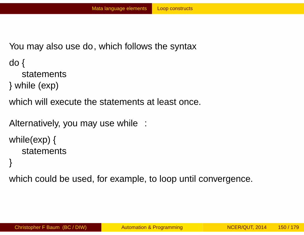
Mata language elements Loop constructs
You may also use do, which follows the syntax
do {statements
} while (exp)
which will execute the statements at least once.
Alternatively, you may use while:
while(exp) {statements
}
which could be used, for example, to loop until convergence.
Christopher F Baum (BC / DIW) Automation & Programming NCER/QUT, 2014 150 / 179
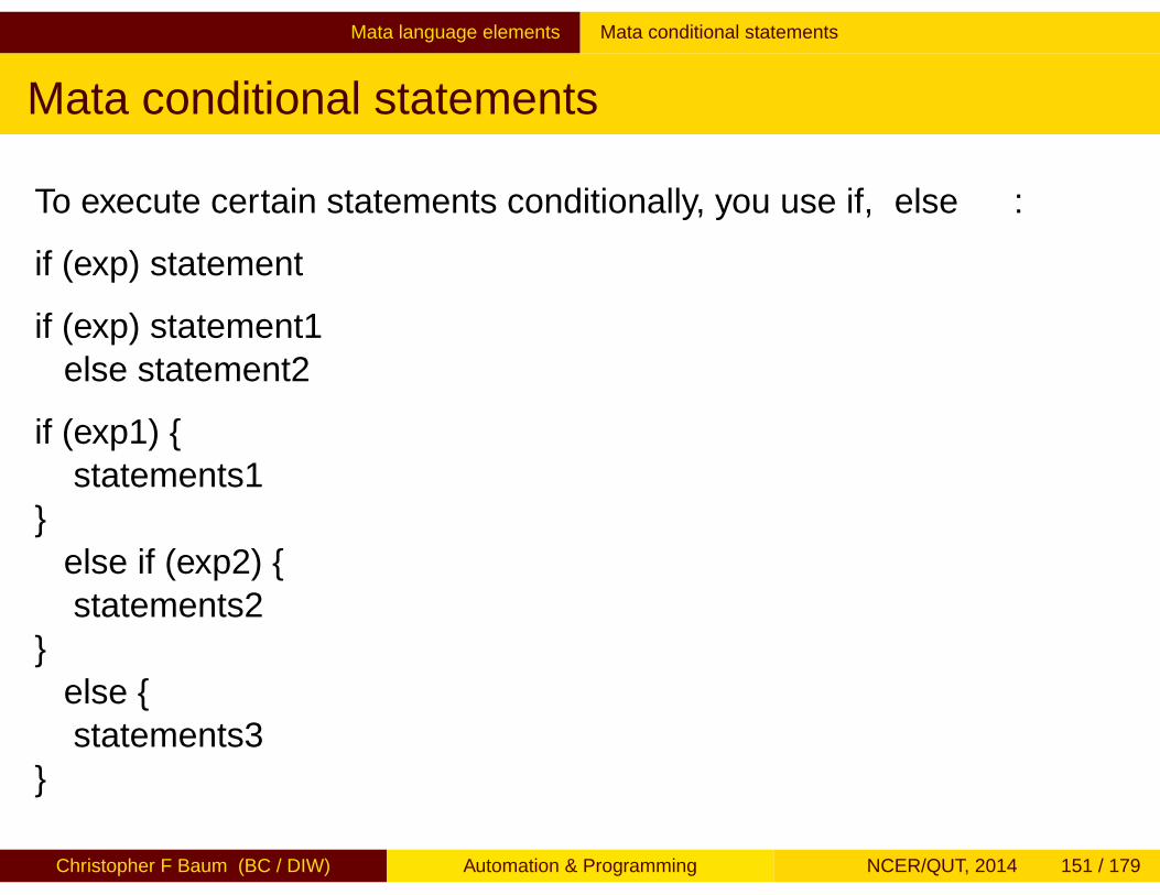
Mata language elements Mata conditional statements
Mata conditional statements
To execute certain statements conditionally, you use if, else:
if (exp) statement
if (exp) statement1else statement2
if (exp1) {statements1
}else if (exp2) {statements2
}else {statements3
}
Christopher F Baum (BC / DIW) Automation & Programming NCER/QUT, 2014 151 / 179

Mata language elements Mata conditional statements
You may also use the conditional a ? b : c, where a is a real scalar.If a evaluates to true (nonzero), the result is set to b, otherwise c. Forinstance,
if (k == 0) dof = n-1else dof = n-k
can be written as
dof = ( k==0 ? n-1 : n-k )
The increment (++) and decrement (−−) operators can be used tomanage counter variables. They may precede or follow the variable.
The operator A # B produces the Kronecker or direct product of A andB.
Christopher F Baum (BC / DIW) Automation & Programming NCER/QUT, 2014 152 / 179

Design of a Mata function Element and organization types
Element and organization types
To call Mata code within an ado-file, you must define a Mata function,which is the equivalent of a Stata ado-file program. Unlike a Stataprogram, a Mata function has an explicit return type and a set ofarguments. A function may be of return type void if it does not need a�return statement. Otherwise, a function is typed in terms of twocharacteristics: its element type and their organization type. Forinstance,
real scalar calcsum(real vector x)
declares that the Mata calcsum function will return a real scalar. It hasone argument: an object x, which must be a real vector.
Christopher F Baum (BC / DIW) Automation & Programming NCER/QUT, 2014 153 / 179

Design of a Mata function Element and organization types
Element types may be real, complex, numeric, string,
pointer, transmorphic. A transmorphic object may be filled withany of the other types. A numeric object may be either real orcomplex. Unlike Stata, Mata supports complex arithmetic.
There are five organization types: matrix, vector, rowvector,
colvector, scalar. Strictly speaking the latter four are just specialcases of matrix. In Stata’s matrix language, all matrices have twosubscripts, neither of which can be zero. In Mata, all but the scalar
may have zero rows and/or columns. Three- (and higher-) dimensionmatrices can be implemented by the use of the pointer element type,not to be discussed further in this talk.
Christopher F Baum (BC / DIW) Automation & Programming NCER/QUT, 2014 154 / 179
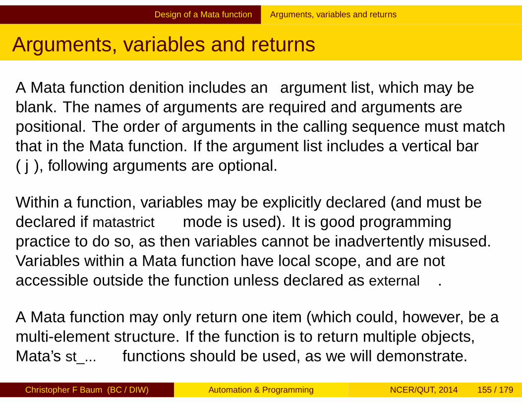
Design of a Mata function Arguments, variables and returns
Arguments, variables and returns
A Mata function definition includes an argument list, which may beblank. The names of arguments are required and arguments arepositional. The order of arguments in the calling sequence must matchthat in the Mata function. If the argument list includes a vertical bar( | ), following arguments are optional.
Within a function, variables may be explicitly declared (and must bedeclared if matastrict mode is used). It is good programmingpractice to do so, as then variables cannot be inadvertently misused.Variables within a Mata function have local scope, and are notaccessible outside the function unless declared as external.
A Mata function may only return one item (which could, however, be amulti-element structure. If the function is to return multiple objects,Mata’s st_... functions should be used, as we will demonstrate.
Christopher F Baum (BC / DIW) Automation & Programming NCER/QUT, 2014 155 / 179
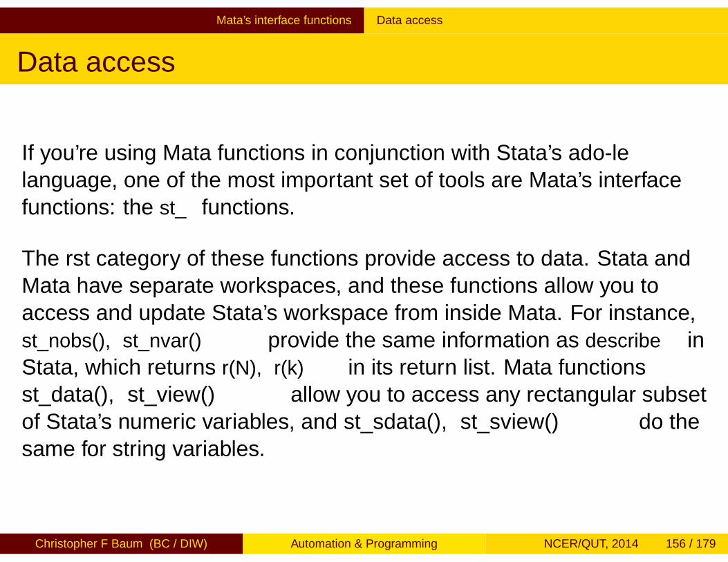
Mata’s interface functions Data access
Data access
If you’re using Mata functions in conjunction with Stata’s ado-filelanguage, one of the most important set of tools are Mata’s interfacefunctions: the st_ functions.
The first category of these functions provide access to data. Stata andMata have separate workspaces, and these functions allow you toaccess and update Stata’s workspace from inside Mata. For instance,st_nobs(), st_nvar() provide the same information as describe inStata, which returns r(N), r(k) in its return list. Mata functionsst_data(), st_view() allow you to access any rectangular subsetof Stata’s numeric variables, and st_sdata(), st_sview() do thesame for string variables.
Christopher F Baum (BC / DIW) Automation & Programming NCER/QUT, 2014 156 / 179

Mata’s interface functions st_view( )
st_view( )
One of the most useful Mata concepts is the view matrix, which as itsname implies is a view of some of Stata’s variables for specifiedobservations, created by a call to st_view(). Unlike most Matafunctions, st_view() does not return a result. It requires threearguments: the name of the view matrix to be created, theobservations (rows) that it is to contain, and the variables (columns).An optional fourth argument can specify touse: an indicator variablespecifying whether each observation is to be included. The statement
st_view(x, ., varname, touse)
states that the previously-declared Mata vector x should be createdfrom all the observations (specified by the missing second argument)of varname, as modified by the contents of touse. In the Stata code,the marksample command imposes any if or in conditions bysetting the indicator variable touse.
Christopher F Baum (BC / DIW) Automation & Programming NCER/QUT, 2014 157 / 179
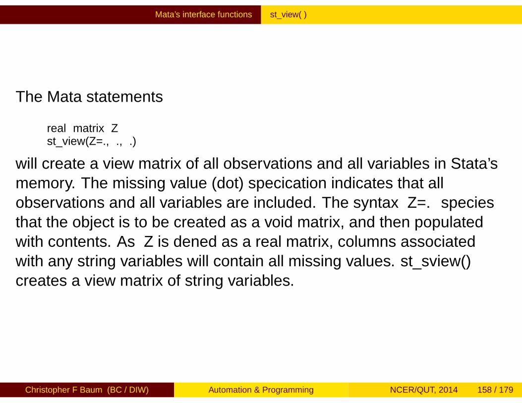
Mata’s interface functions st_view( )
The Mata statements
real matrix Zst_view(Z=., ., .)
will create a view matrix of all observations and all variables in Stata’smemory. The missing value (dot) specification indicates that allobservations and all variables are included. The syntax Z=. specifiesthat the object is to be created as a void matrix, and then populatedwith contents. As Z is defined as a real matrix, columns associatedwith any string variables will contain all missing values. st_sview()creates a view matrix of string variables.
Christopher F Baum (BC / DIW) Automation & Programming NCER/QUT, 2014 158 / 179

Mata’s interface functions st_view( )
If we want to specify a subset of variables, we must define a stringvector containing their names. For instance, if varlist is a string
scalar argument containing Stata variable names,
void foo( string scalar varlist )...
st_view(X=., ., tokens(varlist), touse)
creates matrix X containing those variables.
Christopher F Baum (BC / DIW) Automation & Programming NCER/QUT, 2014 159 / 179

Mata’s interface functions st_data( )
st_data( )
An alternative to view matrices is provided by st_data() andst_sdata(), which copy data from Stata variables into Matamatrices, vectors or scalars:
X = st_data(., .)
places a copy of all variables in Stata’s memory into matrix X.However, this operation requires at least twice as much memory asconsumed by the Stata variables, as Mata does not have Stata’s fullset of 1-, 2-, and 4-byte data types. Thus, although a view matrix canreference any variables currently in Stata’s memory with minimaloverhead, a matrix created by st_data() will consume considerablememory, just as a matrix in Stata’s own matrix language does.
Similar to st_view(), an optional third argument to st_data() canmark out desired observations.
Christopher F Baum (BC / DIW) Automation & Programming NCER/QUT, 2014 160 / 179

Mata’s interface functions Using views to update Stata variables
Using views to update Stata variables
A very important aspect of views: using a view matrix rather thancopying data into Mata with st_data() implies that any changes madeto the view matrix will be reflected in Stata’s variables’ contents. This isa very powerful feature that allows us to easily return informationgenerated in Mata back to Stata’s variables, or create new content inexisting variables.
This may or may not be what you want to do. Keep in mind that anyalterations to a view matrix will change Stata’s variables, just as areplace command in Stata would. If you want to ensure that Matacomputations cannot alter Stata’s variables, avoid the use of views, oruse them with caution. You may use st_addvar() to explicitly createnew Stata variables, and st_store() to populate their contents.
Christopher F Baum (BC / DIW) Automation & Programming NCER/QUT, 2014 161 / 179

Mata’s interface functions Using views to update Stata variables
A Mata function may take one (or several) existing variables and createa transformed variable (or set of variables). To do that with views,create the new variable(s), pass the name(s) as a newvarlist and setup a view matrix.
st_view(Z=., ., tokens(newvarlist), touse)
Then compute the new content as:
Z[., .] = result of computation
It is very important to use the [., .] construct as shown. Z = willcause a new matrix to be created and break the link to the view.
Christopher F Baum (BC / DIW) Automation & Programming NCER/QUT, 2014 162 / 179
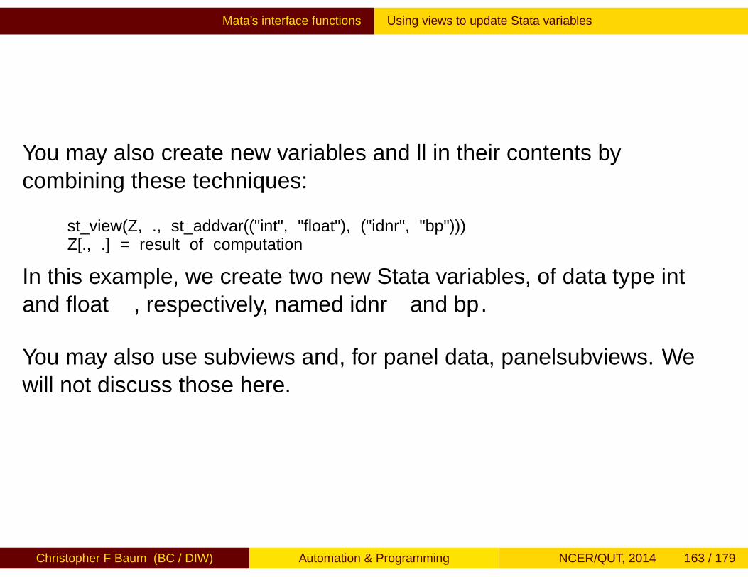
Mata’s interface functions Using views to update Stata variables
You may also create new variables and fill in their contents bycombining these techniques:
st_view(Z, ., st_addvar(("int", "float"), ("idnr", "bp")))Z[., .] = result of computation
In this example, we create two new Stata variables, of data type intand float, respectively, named idnr and bp.
You may also use subviews and, for panel data, panelsubviews. Wewill not discuss those here.
Christopher F Baum (BC / DIW) Automation & Programming NCER/QUT, 2014 163 / 179

Mata’s interface functions Access to locals, globals, scalars and matrices
Access to locals, globals, scalars and matrices
You may also want to transfer other objects between the Stata andMata environments. Although local and global macros, scalars andStata matrices could be passed in the calling sequence to a Matafunction, the function can only return one item. In order to return anumber of objects to Stata—for instance, a list of macros, scalars andmatrices as is commonly found in the return list from an r-classprogram—we use the appropriate st_functions.
For local macros,
contents = st_local("macname")st_local("macname", newvalue )
The first command will return the contents of Stata local macromacname. The second command will create and populate that localmacro if it does not exist, or replace the contents if it does, withnewvalue.
Christopher F Baum (BC / DIW) Automation & Programming NCER/QUT, 2014 164 / 179

Mata’s interface functions Access to locals, globals, scalars and matrices
Along the same lines, functions st_global, st_numscalar andst_strscalar may be used to retrieve the contents, create, orreplace the contents of global macros, numeric scalars and stringscalars, respectively. Function st_matrix performs these operationson Stata matrices.
All of these functions can be used to obtain the contents, create orreplace the results in r( ) or e( ): Stata’s return list andereturn list. Functions st_rclear and st_eclear can be usedto delete all entries in those lists. Read-only access to the c( )objects is also available.
The stata( ) function can execute a Stata command from withinMata.
Christopher F Baum (BC / DIW) Automation & Programming NCER/QUT, 2014 165 / 179

Some examples of Stata–Mata routines A simple Mata function
A simple Mata function
We now give a simple illustration of how a Mata subroutine could beused to perform the computations in a do-file. We consider the sameroutine: an ado-file, mysum3, which takes a variable name and acceptsoptional if or in qualifiers. Rather than computing statistics in theado-file, we call the m_mysum routine with two arguments: the variablename and the ‘touse’ indicator variable.
program define mysum3, rclassversion 13syntax varlist(max=1) [if] [in]return local varname `varlist´marksample tousemata: m_mysum("`varlist´", "`touse´")return scalar N = Nreturn scalar sum = sumreturn scalar mean = mureturn scalar sd = sigma
end
Christopher F Baum (BC / DIW) Automation & Programming NCER/QUT, 2014 166 / 179

Some examples of Stata–Mata routines A simple Mata function
In the same ado-file, we include the Mata routine, prefaced by themata: directive. This directive on its own line puts Stata into Matamode until the end statement is encountered. The Mata routinecreates a Mata view of the variable. A view of the variable is merely areference to its contents, which need not be copied to Mata’sworkspace. Note that the contents have been filtered for missingvalues and those observations specified in the optional if or inqualifiers.
That view, labeled as X in the Mata code, is then a matrix (or, in thiscase, a column vector) which may be used in various Mata functionsthat compute the vector’s descriptive statistics. The computed resultsare returned to the ado-file with the st_numscalar( ) function calls.
Christopher F Baum (BC / DIW) Automation & Programming NCER/QUT, 2014 167 / 179

Some examples of Stata–Mata routines A simple Mata function
version 13mata:void m_mysum(string scalar vname,
string scalar touse)
st_view(X, ., vname, touse)mu = mean(X)st_numscalar("N", rows(X))st_numscalar("mu", mu)st_numscalar("sum" ,rows(X) * mu)st_numscalar("sigma", sqrt(variance(X)))
end
Christopher F Baum (BC / DIW) Automation & Programming NCER/QUT, 2014 168 / 179

Some examples of Stata–Mata routines A multi-variable function
A multi-variable function
Now let’s consider a slightly more ambitious task. Say that you wouldlike to center a number of variables on their means, creating a new setof transformed variables. Surprisingly, official Stata does not havesuch a command, although Ben Jann’s center command does so.Accordingly, we write Stata command centervars, employing a Matafunction to do the work.
Christopher F Baum (BC / DIW) Automation & Programming NCER/QUT, 2014 169 / 179
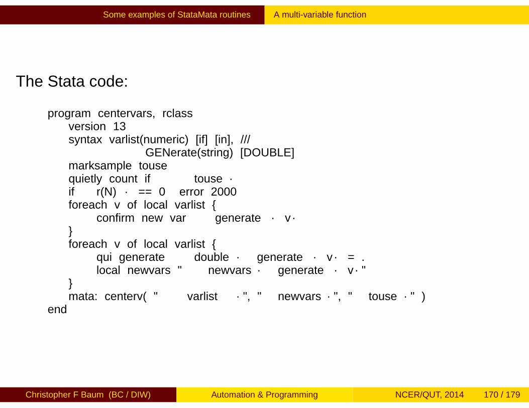
Some examples of Stata–Mata routines A multi-variable function
The Stata code:
program centervars, rclassversion 13syntax varlist(numeric) [if] [in], ///
GENerate(string) [DOUBLE]marksample tousequietly count if `touse´if `r(N)´ == 0 error 2000foreach v of local varlist {
confirm new var `generate´`v´}foreach v of local varlist {
qui generate `double´ `generate´`v´ = .local newvars "`newvars´ `generate´`v´"
}mata: centerv( "`varlist´", "`newvars´", "`touse´" )
end
Christopher F Baum (BC / DIW) Automation & Programming NCER/QUT, 2014 170 / 179

Some examples of Stata–Mata routines A multi-variable function
The file centervars.ado contains a Stata command, centervars,that takes a list of numeric variables and a mandatory generate()option. The contents of that option are used to create new variablenames, which then are tested for validity with confirm new var, andif valid generated as missing. The list of those new variables isassembled in local macro newvars. The original varlist and the listof newvars is passed to the Mata function centerv() along withtouse, the temporary variable that marks out the desiredobservations.
Christopher F Baum (BC / DIW) Automation & Programming NCER/QUT, 2014 171 / 179

Some examples of Stata–Mata routines A multi-variable function
The Mata code:
version 13mata:void centerv( string scalar varlist, ///
string scalar newvarlist,string scalar touse)
{real matrix X, Zst_view(X=., ., tokens(varlist), touse)st_view(Z=., ., tokens(newvarlist), touse)Z[ ., . ] = X :- mean(X)
}end
Christopher F Baum (BC / DIW) Automation & Programming NCER/QUT, 2014 172 / 179
Some examples of Stata–Mata routines A multi-variable function
In the Mata function, tokens( ) extracts the variable names fromvarlist and places them in a string rowvector, the form needed byst_view . The st_view function then creates a view matrix, X,containing those variables and the observations selected by if and inconditions.
The view matrix allows us to both access the variables’ contents, asstored in Mata matrix X, but also to modify those contents. The colonoperator (:-) subtracts the vector of column means of X from the data.Using the Z[,]= notation, the Stata variables themselves aremodified. When the Mata function returns to Stata, the contents anddescriptive statistics of the variables in varlist will be altered.
Christopher F Baum (BC / DIW) Automation & Programming NCER/QUT, 2014 173 / 179
Some examples of Stata–Mata routines A multi-variable function
One of the advantages of Mata use is evident here: we need not loopover the variables in order to demean them, as the operation can bewritten in terms of matrices, and the computation done very efficientlyeven if there are many variables and observations. Also note thatperforming these calculations in Mata incurs minimal overhead, as thematrix Z is merely a view on the Stata variables in newvars. Onecaveat: Mata’s mean() function performs listwise deletion, like Stata’scorrelate command.
Christopher F Baum (BC / DIW) Automation & Programming NCER/QUT, 2014 174 / 179

Some examples of Stata–Mata routines Passing a function to Mata
Passing a function to Mata
Let’s consider adding a feature to centervars: the ability totransform variables before centering with one of several mathematicalfunctions (abs(), exp(), log(), sqrt()). The user will provide thename of the desired transformation, which defaults to the identitytransformation, and Stata will pass the name of the function (actually, apointer to the function) to Mata. We call this new commandcentertrans.
Christopher F Baum (BC / DIW) Automation & Programming NCER/QUT, 2014 175 / 179

Some examples of Stata–Mata routines Passing a function to Mata
The Stata code:program centertrans, rclass
version 13syntax varlist(numeric) [if] [in], ///
GENerate(string) [TRans(string)] [DOUBLE]marksample tousequietly count if ‘touse’if ‘r(N)’ == 0 error 2000local trops abs exp log sqrtif "‘trans’" == "" {local trfn "mf_iden"
}else {local ntr : list posof "‘trans’" in tropsif !‘ntr’ {display as err "Error: trans must be chosen from ‘trops’"error 198}
local trfn : "mf_‘trans’"}foreach v of local varlist {
confirm new var ‘generate’‘trans’‘v’}foreach v of local varlist {
qui generate ‘double’ ‘generate’‘trans’‘v’ = .local newvars "‘newvars’ ‘generate’‘trans’‘v’"
}mata: centertrans( "‘varlist’", "‘newvars’", &‘trfn’(), "‘touse’" )
end
Christopher F Baum (BC / DIW) Automation & Programming NCER/QUT, 2014 176 / 179

Some examples of Stata–Mata routines Passing a function to Mata
In Mata, we must define “wrapper functions" for the transformations, aswe cannot pass a pointer to a built-in function. We define trivialfunctions such as
function mf_log(x) return(log(x))
which defines the mf_log() scalar function as taking the log of itsargument.
The Mata function centertrans() receives the function argument as
pointer(real scalar function) scalar f
To apply the function, we use
Z[ ., . ] = (*f)(X)
which applies the function referenced by f to the elements of thematrix X. The Z matrix is then demeaned as before.
Christopher F Baum (BC / DIW) Automation & Programming NCER/QUT, 2014 177 / 179
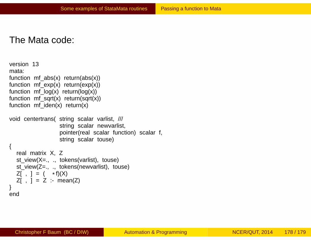
Some examples of Stata–Mata routines Passing a function to Mata
The Mata code:
version 13mata:function mf_abs(x) return(abs(x))function mf_exp(x) return(exp(x))function mf_log(x) return(log(x))function mf_sqrt(x) return(sqrt(x))function mf_iden(x) return(x)
void centertrans( string scalar varlist, ///string scalar newvarlist,pointer(real scalar function) scalar f,string scalar touse)
{real matrix X, Zst_view(X=., ., tokens(varlist), touse)st_view(Z=., ., tokens(newvarlist), touse)Z[ , ] = (*f)(X)Z[ , ] = Z :- mean(Z)
}end
Christopher F Baum (BC / DIW) Automation & Programming NCER/QUT, 2014 178 / 179

Some examples of Stata–Mata routines Passing a function to Mata
For more detail on Mata, see Chapters 13–14 of An Introduction toStata Programming; Bill Gould’s Stata Conference talk, “Mata: theMissing Manual” at http://repec.org; and Ben Jann’s morematapackage, available from the SSC Archive.
Christopher F Baum (BC / DIW) Automation & Programming NCER/QUT, 2014 179 / 179