boston college the graduate school of arts and sciences
TRANSCRIPT
Boston College
The Graduate School of Arts and Sciences
Department of Physics
Symmetry and topology in condensed matter physics
a dissertation
by
XU YANG
submitted in partial fulfillment of the requirements
for the degree of
Doctor of Philosophy
MAY 2021

© copyright by XU YANG2021

Symmetry and topology in condensed matter physics
XU YANG
Dissertation advisor: Dr. Ying Ran
AbstractRecently there has been a surging interest in the topological phases of matter, including
the symmetry-protected topological phases, symmetry-enriched topological phases, and
topological semimetals. This thesis is aiming at finding new ways of searching and probing
these topological phases of matter in order to deepen our understanding of them.
The body of the thesis consists of three parts. In the first part, we study the search
of filling-enforced topological phases of matter in materials. It shows the existence of
symmetry-protected topological phases enforced by special electron fillings or fractional
spin per unit-cell. This is an extension of the famous Lieb-Schultz-Mattis theorem. The
original LSM theorem states that the symmetric gapped ground state of the system must
exhibit topological order when there’s fractional spin or fractional electron filling per unit-
cell. However, the LSM theorem can be circumvented when commensurate magnetic flux
is present in the system, which enlarge the unit-cells to accommodate integer numbers of
electrons. We utilize this point to prove that the ground state of the system must be a
symmetry-protected topological phase when magnetic translation symmetry is satisfied,
which we coin the name “generalized LSM theorem”. The theorem is proved using two
different methods. The first proof is to use the tensor network representation of the ground

state wave-function. The second proof consists of a physical argument based on the idea of
entanglement pumping. As a byproduct of this theorem, a large class of decorated quantum
dimer models are introduced, which satisfy the condition of the generalized LSM theorem
and exhibit SPT phases as their ground states.
In part II, we switch to the nonlinear response study of Weyl semimetals. Weyl semimet-
als (WSM) have been discovered in time-reversal symmetric materials, featuring monopoles
of Berry’s curvature in momentum space. WSM have been distinguished between Type-I
and II where the velocity tilting of the cone in the later ensures a finite area Fermi sur-
face.To date it has not been clear whether the two types results in any qualitatively new
phenomena. In this part we focus on the shift-current response (σshift(ω)), a second or-
der optical effect generating photocurrents. We find that up to an order unity constant,
σshift(ω) ∼ e3
h21ω
in Type-II WSM, diverging in the low frequency ω → 0 limit. This is in
stark contrast to the vanishing behavior (σshift(ω) ∝ ω) in Type-I WSM. In addition, in
both Type-I and Type-II WSM, a nonzero chemical potential µ relative to nodes leads to
a large peak of shift-current response with a width ∼ |µ|/~ and a height ∼ e3
h1|µ| , the latter
diverging in the low doping limit. We show that the origin of these divergences is the sin-
gular Berry’s connections and the Pauli-blocking mechanism. Similar results hold for the
real part of the second harmonic generation, a closely related nonlinear optical response.
In part III, we propose a new kind of thermo-optical experiment: the nonreciprocal
directional dichroism induced by a temperature gradient. The nonreciprocal directional
dichroism effect, which measures the difference in the optical absorption coefficient be-
tween counterpropagating lights, occurs only in systems lacking inversion symmetry. The
introduction of temperature-gradient in an inversion-symmetric system will also yield non-

reciprocal directional dichroism effect. This effect is then applied to quantum magnetism,
where conventional experimental techniques have difficulty detecting magnetic mobile ex-
citations such as magnons or spinons exclusively due to the interference of phonons and
local magnetic impurities. A model calculation is presented to further demonstrate this
phenomenon.

Acknowledgments
First off, I wish to express my deepest gratitude to my advisor, Prof. Ying Ran. Nu-
merous topics have I worked on and many extensive and intensive discussions with him are
of the most joyous moments during my graduate years. His guidance in always asking the
right question, in never taking any unexamined opinion for granted, has largely shaped my
view of physics. Besides, his numerous advice on my career path and personal life have
helped me greatly. I am truly lucky to have him as my advisor.
I would also like to thank the rest of my thesis committee: Prof. Ziqiang Wang, Prof.
Ken Burch and Prof. Fazel Tafti. I thank Prof. Wang for many assistance during the
past years including course selection, research proposal exam, etc.. I thank Prof. Burch for
collaborations and solid state physics knowledge I have learned from him during various
discussions. I thank Prof. Tafti for discussions and solid state physics I have learned from
his class and also for being a committee member in my research proposal exam.
I am deeply thankful to Prof. Masaki Oshikawa for his hospitality during my visit in
Japan, and for the many deep physics insights he has imparted to me and for his help
during my postdoc application. And I would also like to thank Prof. Ashvin Vishwanath
for the collaboration and for his leadership in the field of condensed matter physics which
deeply affects my own research. I am also thankful to Prof. Gang Chen for collaborations,
science discussions, and his hospitality during my visit in Hong Kong. I am also grateful to
the faculty members of the Physics Department, especially, Prof. Michael Graf, Prof. Ilija
Zeljkovic, Prof. Xiao Chen, Prof. P. Bakshi. I am also grateful to staffs in the department,
vi

epecially Jane, Nancy, Sile and Scott. Their kindness to me has made my stay at Boston
College a very pleasant experience.
I also want to thank my colleagues and collaborators, both at Boston College and else-
where. Especially I would like to thank Shenghan Jiang, Kun Jiang, Tong Yang, Xiaodong
Hu, Joshuah Heath and Hanlong Fang. The uncountable numbers of discussions on physics,
metaphysics and pseudophysics and delicious meals shared with them have shaped both
my mind and my body. I would also like to thank He Zhao, Zheng Ren, Lidong Ma, Yiping
Wang, Hong Li at Boston College; and Xinqiang Cai, Zhicheng Yang, Yahui Zhang, Yuzi
He, Yuwen Hu, Yuan Yao and Chunxiao Liu at other institutes, and my friends outside of
physics, Yuansheng Zhou, Ting Zhu, Teng Bian, Zejie Yu, Zhichuang Sun, Siyi Ye, Qi Guo,
Xiang Gao, Shiping Wang, Yongtao Wang, the happy moments spent with whom prevent
me from getting permanent head demage (a.k.a, PHD).
Finally, I would like to thank my parents, whose enduring love and never-ceasing support
make me become what I want to be. And I would like to thank God our Lord, “for you, O
Lord, have made me glad by your work; at the works of your hands I sing for joy.”1
1Psalm 92:4, ESV
vii

To My Parents.
viii

Contents
1 General prologue 1
1.1 Overview of condensed matter physics . . . . . . . . . . . . . . . . . . . . 1
1.2 The advent of topological era . . . . . . . . . . . . . . . . . . . . . . . . . 5
1.3 Structure of the thesis . . . . . . . . . . . . . . . . . . . . . . . . . . . . . 11
2 Dyonic Lieb-Schultz-Mattis theorem 20
2.1 Overview . . . . . . . . . . . . . . . . . . . . . . . . . . . . . . . . . . . . 20
2.2 A simple model realizing SPT phase . . . . . . . . . . . . . . . . . . . . . 25
2.3 Main Results . . . . . . . . . . . . . . . . . . . . . . . . . . . . . . . . . . 34
2.3.1 Examples . . . . . . . . . . . . . . . . . . . . . . . . . . . . . . . . 38
2.4 Decorated Quantum Dimer Models for SPT phases . . . . . . . . . . . . . 42
2.4.1 G = SO(3)× ZIsing2 , a spin-1/2 per unit cell . . . . . . . . . . . . . 42
2.4.2 G = ZT2 × ZIsing
2 . . . . . . . . . . . . . . . . . . . . . . . . . . . . 51
2.5 Proof of Theorems . . . . . . . . . . . . . . . . . . . . . . . . . . . . . . . 55
2.5.1 Entanglement Pumping argument . . . . . . . . . . . . . . . . . . . 56
2.5.2 Symmetry-enforced constraints on SPT cocycles . . . . . . . . . . . 58
2.5.3 Generic constructions of Symmetry-enforced SPT wavefunctions . . 58
ix
2.6 Discussion . . . . . . . . . . . . . . . . . . . . . . . . . . . . . . . . . . . . 59
2.7 Appendices . . . . . . . . . . . . . . . . . . . . . . . . . . . . . . . . . . . 61
2.7.1 Perturbation study of the decorated Balents-Fisher-Girvin model . 61
2.7.2 Theorem-I as a special case of Theorem-II . . . . . . . . . . . . . . 63
2.7.3 A brief introduction to symmetric tensor network representation of
SPT phases . . . . . . . . . . . . . . . . . . . . . . . . . . . . . . . 66
2.7.4 The projective representation carried by a g-symmetry-defect . . . 69
2.7.5 Consequence of the magnetic translation symmetry in tensor-network
formulation . . . . . . . . . . . . . . . . . . . . . . . . . . . . . . . 72
2.7.6 Generic constructions of symmetry-enforced SPT tensor-network wave-
functions . . . . . . . . . . . . . . . . . . . . . . . . . . . . . . . . 76
3 Divergent bulk photovoltaic effect in Weyl semimetals 93
3.1 Introduction . . . . . . . . . . . . . . . . . . . . . . . . . . . . . . . . . . . 93
3.2 Main results . . . . . . . . . . . . . . . . . . . . . . . . . . . . . . . . . . . 97
3.3 Appendices . . . . . . . . . . . . . . . . . . . . . . . . . . . . . . . . . . . 104
3.3.1 Shift current in type-I Weyl semi-metal . . . . . . . . . . . . . . . . 104
3.3.2 Analytical formula for the shift current in Weyl semi-metal with
tilting and doping in low-frequency limit . . . . . . . . . . . . . . . 107
3.3.3 Analytical formula for the second-harmonic-generation in Weyl semi-
metal with tilting and doping in low-frequency limit . . . . . . . . 110
4 Nonreciprocal directional dichroism induced by a temperature gradient
as a probe for mobile spin dynamics in quantum magnets 119
x

4.1 Introduction . . . . . . . . . . . . . . . . . . . . . . . . . . . . . . . . . . . 119
4.2 The effect of TNDD . . . . . . . . . . . . . . . . . . . . . . . . . . . . . . 120
4.3 Discussion and conclusion . . . . . . . . . . . . . . . . . . . . . . . . . . . 130
4.4 Appendices . . . . . . . . . . . . . . . . . . . . . . . . . . . . . . . . . . . 131
4.4.1 Localized modes . . . . . . . . . . . . . . . . . . . . . . . . . . . . 131
4.4.2 Spin-orbit coupling and the estimate of TNDD response . . . . . . 133
4.4.3 Details of the mean-field calculation for TNDD . . . . . . . . . . . 137
xi

List of Figures
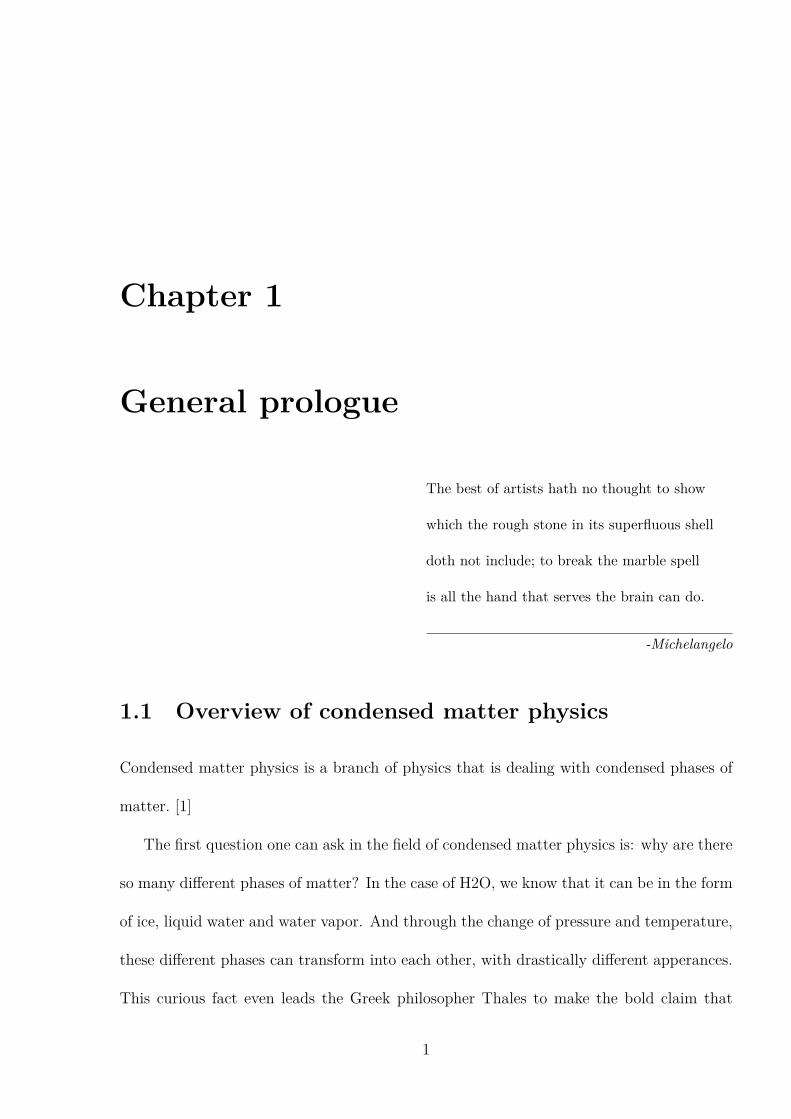
1.1 The p− T phase diagram of water. The first-order liquid-gas transition line
ends at the critical point with Tc = 647K,Pc = 2.2 ∗ 108Pa. The phase
transition at the critical point becomes a second-order one, with continuous
change of density and any other first order derivatives of the thermodynamic
potential. Beyond the critical point, there is no phase transition between
liquid water and water vapor. . . . . . . . . . . . . . . . . . . . . . . . . . 2
2.1 (color online) Degrees of freedom in the decorated BFG model. The Ising
d.o.f. σI live on the honeycomb lattice and the spin d.o.f. Si lives on the
Kagome lattice. The Ising coupling signs sIJ = +1 on red bonds, and
sIJ = −1 on blue bonds. The thick red bonds represent the “y-odd zigzag
chains” used in Eq. (2.14) . . . . . . . . . . . . . . . . . . . . . . . . . . . 26
xii

2.2 (color online) (a) Schematic phase diagram of the decorated BFG model
by tuning λ. We have already fixed Jz ≫ J⊥, h. In the limit λ → 0 the
Ising layer is decoupled and the ground state is just that of the original
BFG model with Z2 topological order. This is an SET state with spinon
carrying Sz = 1/2. When λ is tuned to be within the parameter regime
where Jz ≫ λ ≫ J⊥, h and h2
λ2 ≫ J⊥Jz
, we have an SPT state with Ising
defect carrying Sz = 1/2 as discussed in the main text. There is a possible
direct phase transition triggered by the condensation of Ising-odd visons at
some intermediate λc. (b) A schematic view of vison condensation. The
honeycomb lattice where Ising d.o.f. lives is shown and the spin d.o.f. lives
in the bond center. Two visons are created at the ends I, J of the string
operator σzIσ
zJ
j∏k=i
−→ 2Szk . with Sz
k runs over all the black dot shown in the
graph. Alternatively we can view the string operator as the product of
bond variable Szi σ
zIσ
zK along the thick blue bonds. Due to the constraint
Szi (sIKσ
zIσ
zK) = 1, the string operator will yield a factor (product of sIK ’s
along the thick blue bonds) when acting on the ground state wave-function,
which means the visons are condensed and the topological order is killed.
Note that the condensed visons in the present case are dressed by local σz
operator and hence carry the quantum number of Z2 Ising symmetry, which
result in an SPT state. . . . . . . . . . . . . . . . . . . . . . . . . . . . . . 29
xiii

2.3 (color online) An pair of Ising defects (only one is shown) is created at the
end points of the branch cut (dashed black line) after modifying the original
Hamiltonian H in Eq.(2.5) into H ′. The sign sIJ is flipped in H ′ along the
branch cut comparing with the original model. (red bond: sIJ = +1, blue
bond: sIJ = −1) For any loop C enclosing the Ising defect as the gray loop
shown here, the product∏sIJ around the loop flips sign comparing with
the original model. In order that H ′binding does not cost extra energy, the
spin should be flipped wherever sIJ changes its sign. As a result, the total
Sz around the loop C is changed by an odd integer. The result is that Ising
defect is topologically bound with a half-integer spin. See the discussion in
the main text. . . . . . . . . . . . . . . . . . . . . . . . . . . . . . . . . . . 32
2.4 (color online) The Ising d.o.f. σ live on the honeycomb lattice and the spin
d.o.f. τ lives on the triangular lattice. The Ising coupling signs sIJ = +1
on red bonds, and sIJ = −1 on blue vertical bonds. The thick red bonds
represent the “y-odd zigzag chains” used in Eq.(2.25,2.36 ). The thick gray
horizontal bonds on the triangular lattice represent the “y-odd rows” used
in Eq.(2.36). . . . . . . . . . . . . . . . . . . . . . . . . . . . . . . . . . . 43
2.5 To construct model in Eq.(2.35), the dimer states living on the nearest
neighbor bonds on the triangular lattice have a spatial dependent pattern:
the dimer states living on the dashed bonds are defined in Eq.(2.37), and
those living on the dotted bonds are defined in Eq.(2.38). . . . . . . . . . . 53
xiv

2.6 Illustration of adiabatically separating a pair of g-defect/antidefect along
the x-direction with g3 = I. For simplicity, one may imagine Hamiltonian
to host nearest neighbor (NN) terms. Along the x-direction, due to the
magnetic translation symmetry Eq.(2.16), the NN interactions on the verti-
cal bonds have a three-unit-cell periodicity (solid,dashed and dotted bonds).
While the g-defect crosses the entanglement cut at x0 + 1/2, the Hamilto-
nian along the branch cut (dashed gray line) is effectively translated along
x-direction by one unit cell. After separating such pairs of defects for every
row, the final Hamiltonian is related to the original Hamiltonian by T orig.x . 57
2.7 The decomposition of global IGG into plaquette IGG. λ’s from different
plaquettes commutes with each other, and the action of any two λ’s in the
same plaquette leave the tensor invariant. . . . . . . . . . . . . . . . . . . 68
2.8 An example of g-defect line. The g-defect line is obtained by inserting
Wg on only one side of the virtual legs crossed by the red dashed line.
The tensors close to the defect core should be revised in order to make
the tensor wave-function symmetric and non-vanishing. Following the usual
convention, we say that the defect line always points from g−1-defect to g-
defect, and we always insert Wg to the left when one goes forward along the
line. Therefore in the figure we can identify the right end as the g-defect
(remember Wg(d) = Wg(u)−1). The grey area encloses a g-defect and we
can to measure its projective representation through the action of η′(a, b) on
the boundary virtual legs, see the discussion in the main text. . . . . . . . 81
xv
2.9 Invariance of the wave-function under U g(a). In the figure we can see that
Wa = [λa(g)](d) ·Wa where the defect line crosses the boundary and Wa =
Wa elsewhere. Such a definition ensures that no boundary excitations are
created by acting U g(a) (for the moment we do not care about what happens
at the defect core). In deriving the second figure, we have used the invariance
of the tensor under Waa, the identity WaW−1g = W−1
g ξa(g)Wa and invariance
of the tensor under plaquette IGG λa(g). . . . . . . . . . . . . . . . . . . . 82
2.10 Measurement of projective representation carried by g-defect. From Eq. (2.72),
we know that η(a, b) = λa(g) ·Waa λb(g) · η(a, b) · λ−1ab where the boundary
is crossed by the defect line and η(a, b) = η(a, b) elsewhere. In the first
equality we have used Eq. (2.71). In the second equality we have used the
decomposition of η′(a, b) and Eq. (2.66). In the third equality we have used
the tensor invariance under plaquette IGG. In the last equality we have used
the identity λ(r)−1 ·W−1g = W−1
g ·Wg λ(r)−1 and the tensor invariance under
plaquette IGG. . . . . . . . . . . . . . . . . . . . . . . . . . . . . . . . . . 83
2.11 The definition of phase-gauge transformation W (α(a, b)). . . . . . . . . . 84
2.12 The decomposition rule of WTxTxW (α(a, b))·W (α(a, b))−1 (LHS) as a product
of plaquette IGG λ(α(a, b)) (RHS). . . . . . . . . . . . . . . . . . . . . . . 84
2.13 The original tensor before insertion of g-defect is required to be invariant
under the revised symmetry operation and the revised plaquette IGG. . . . 85
xvi

2.14 (a) The definition of the new tensor T (x,y) after the insertion of [Wg(u)]x
to the upper leg of every original tensor T (x,y). (b) The new translation
operationWTxTx. It can be readily checked that T (x,y) is invariant under such
translation. Note that we have Tx = gyT orig.x , Ty = T orig.
y and WTy = 1. (c)
The new on-site symmetry operation Waa. It is shown in Fig. 2.15 that T (x,y)
is invariant under such symmetry operation. (d) The new plaquette IGG for
the new tensor T (x,y). As before, λ’s from different plaquettes commute with
each other, and the action of any two λ’s in the same plaquette leave the
tensor invariant. The tensor T (x,y) invariance under plaquette IGGs follows
trivially from Fig. 2.13. . . . . . . . . . . . . . . . . . . . . . . . . . . . . . 86
2.15 The revised tensor T (x, y) is invariant under the newly-defined symmetry
operation. The first equality comes from the commutation relation WaWxg =
W xg ξa(g,−x)Wa. In the second equality we have used the invariance of tensor
under Wa as shown in Fig. 2.13 and the decomposition of ξa(g,−x). In the
third equality we have used the identity λa(g,−x)(l) =Wgg [λa(g,−x−1)](l)·
λa(g)(l). And we have also used the invariance of tensor under plaquette
IGG as in Fig. 2.14 in the third and fourth equalities. . . . . . . . . . . . . 87
xvii

2.16 Every site-tensor carries a projective representation characterized by [δωg (a, b)]−1.
We show this by acting WaaWbb(Wabab)−1 on both the physical legs and the
virtual legs of tensor T (x,y), which should leave the tensor invariant without
generating any phase. But from the calculation we find that the action on
vitrual legs will contribute a factor δωg (a, b), therefore the representation on
the physical legs are D(a) ·D(b) = [δωg (a, b)]−1D(ab), i.e., they are projected
onto the D2(a) sector with projective representation. In the calculation
above, we have used Eq. (2.95) in the first equality. And we have used the
invariance of the tensor under the plaquette IGG defined in Fig. 2.14 in the
second equality. . . . . . . . . . . . . . . . . . . . . . . . . . . . . . . . . . 88
3.1 (color online) Considering the µ = 0 situation, in (a),(d) we schematically
plot the dispersion relations near a Type-I (Type-II) Weyl node. At zero
temperature, the momentum space surfaces contributing to JDOS (defined
in Eq.(3.7)) are qualitatively different in (b) Type-I WSM and (e) Type-II
WSM, leading to drastically different scaling behaviors of σshift shown in
(c),(f). . . . . . . . . . . . . . . . . . . . . . . . . . . . . . . . . . . . . . . 97
3.2 (color online) At T = 0, the quasi-universal (i.e., µ-independent) line shapes
of the doping-induced peaks of σshift in Type-I (top) and Type-II(bottom)
WSM based on results Eq.(3.9) of linearly dispersive nodes. The peak’s
frequency range has been re-scaled by a µ factor and its height has been
re-scaled by a 1/µ factor, the latter diverges in the low doping limit. . . . . 98
xviii

3.3 (color online) Numerically computed σzxxshift(ω) using the full tight-binding
model Eq.(3.11) with parameters in the main text (squares and triangles),
comparing with analytic linear-node results after summing over four Weyl
nodes σlinearnode (ω) (dashed lines). At zero doping, (a): σshift ∝ ω at T = 0
in Type-I WSM in the low frequency regime; a finite temperature partially
plays the role of doping and induces a peak of σshift whose width ∝ T and
height ∝ 1/T (see supplemental material Fig.3.4); (d): σshift ∝ 1/ω at
T = 0 in Type-II WSM, fully consistent with the result Eq.(3.8) within the
linear approximation. This divergence is truncated by a finite temperature
below ~ω ∼ 5kBT . (b)(c)(e)(f): At finite dopings σshift feature large peaks
whose width ∝ µ and height ∝ 1/µ. At T = 0 these large peaks are well
captured by Eq.(3.8) (the slight deviations for µ = 0.1t cases are due to
expected band-bending effects.). At kBT = 0.02t the peaks for µ = 0.02t
cases are strongly smeared out, while those for µ = 0.1t are quantitatively
reduced. . . . . . . . . . . . . . . . . . . . . . . . . . . . . . . . . . . . . . 113
3.4 At zero doping µ = 0, based on the linear-node result Eq.(3.35), we find
that a finite temperature induces a peak of σshift in Type-I WSM (left), and
truncate the 1/ω divergence in Type-II WSM(right) when ~ω ∼ kBT . Note
that the frequency range is re-scaled by a kBT factor while σshift is re-scaled
by a 1/kBT factor. The line shapes of these curves only depend on W but
independent of kBT . . . . . . . . . . . . . . . . . . . . . . . . . . . . . . . 114
xix
4.1 (a): A schematic illustration of the TNDD effect: in the presence of a tem-
perature gradient, the optical absorption coefficients for counterpropagating
lights become different, which essentially probes the joint density of states of
mobile magnetic excitations. (b) A Kagome lattice and the Dzyaloshinskii–
Moriya vectors Dij. . . . . . . . . . . . . . . . . . . . . . . . . . . . . . . . 126
4.2 The Schwinger boson band dispersion (blue solid lines) for the mean-field
Hamiltonian Eq.(4.9) of Sachdev’s Q1 = Q2 Z2 QSL with parameters A = 1,
Dz = Dp = 0.1J , and µ = −1.792J . The low energy band-1 near the Γ point
is well described by the relativistic dispersion Eq.(4.10) with gap ∆ = 0.16J
(red line). The two-spinon (red dots at ±k) contribution to the TNDD
response computed in Eq.(4.11) and App.4.4.3 is illustrated. . . . . . . . . 128
4.3 The bosonic two-spinon contribution to TNDD spectra of Sachdev’sQ1 = Q2
Z2 QSL Eq.(4.9) at the temperature kBT = 0.7∆ (solid black line) and
kBT = 0.4∆ (solid red line), together with the two-spinon joint density of
states (dashed blue line). . . . . . . . . . . . . . . . . . . . . . . . . . . . . 129
xx

4.4 The fit log(Wq,p/[py ·(ζea4gsµB)]) = log(u0)−√E2
1,q −∆2/∆ (i.e., Eq.(4.31)
with u = uy = u0ζea4gsµB y) with only one fitting parameter u0. In
each case 696 data points with both√E2
1,p −∆2/∆ and√E2
1,q −∆2/∆
between 0.5 and 1.7 are plotted. Since many data points are related by the
lattice symmetry and/or share the same momentum q (but different p), the
visibly different data points are much fewer. We set A = 1, and consider
three cases of different SOC strength: case-(a): Dz = Dp = 0.025J (and
µ = −1.752J); case-(b): Dz = Dp = 0.05J (and µ = −1.765J); case-(c)
Dz = Dp = 0.1J (and µ = −1.792J). Notice that for each case the chemical
potential µ is tuned so that the spinon gap is fixed to be ∆ = 0.16J . As
shown in this figure, we numerically find that u0 = 0.0378 in case-(a),
u0 = 0.151 = 0.0378 · 3.99 in case-(b), and u0 = 0.603 = 0.151 · 3.99 in
case-(c). The scaling u0 ∝ (D/J)2 is confirmed. . . . . . . . . . . . . . . . 141
xxi
Chapter 1
General prologue
The best of artists hath no thought to show
which the rough stone in its superfluous shell
doth not include; to break the marble spell
is all the hand that serves the brain can do.
-Michelangelo
1.1 Overview of condensed matter physics
Condensed matter physics is a branch of physics that is dealing with condensed phases of
matter. [1]
The first question one can ask in the field of condensed matter physics is: why are there
so many different phases of matter? In the case of H2O, we know that it can be in the form
of ice, liquid water and water vapor. And through the change of pressure and temperature,
these different phases can transform into each other, with drastically different apperances.
This curious fact even leads the Greek philosopher Thales to make the bold claim that
1

Figure 1.1: The p − T phase diagram of water. The first-order liquid-gas transition line
ends at the critical point with Tc = 647K,Pc = 2.2 ∗ 108Pa. The phase transition at the
critical point becomes a second-order one, with continuous change of density and any other
first order derivatives of the thermodynamic potential. Beyond the critical point, there is
no phase transition between liquid water and water vapor.
everything is made of water. [2] Here’s a twist: the difference between liquid water and
water vapor is actually pretty vague. Usually one would differentiate between liquid water
and water vapor through the process of evaporation, which is a first-order transition at
which their densities have an abrupt jump. But the p− T phase diagram shows that this
transition line ends at one point, where the density-difference is zero, and beyond which
there’s no clear distinction between liquid water and water vapor. Are they truly different
phases or just the same kind of phase? [1]
Another interesting point associated with phases of matter is as follows. We know from
2

our ordinary experience that liquid and gas are isotropic and uniform (in mathematical
language it means that they are symmetric under the SO(3) spatial rotation and continuous
translation along three directions). At low enough temperature, usually the liquid will form
a crystal, which breaks the SO(3) rotation and continuous translation down to discrete
rotations and discrete translation. This is indeed an astonishing effect, since we know that
the law of electromagnetic force (the dominating force between the atomic scale and the
everyday scale) is apparently isotropic. From quantum mechanics, we also know that the
eigenstates of any Hamiltonian with symmetry G can always be made to be symmetric with
respect to G [3]. There seems no reason for nature to choose a set of non-symmetric states
as the basis in the degenerate space. Let’s take the example of Ising symmetry-breaking in
the transverse-field Ising model as an illustration. [5]
H =∑i
−JSzi S
zi+1 − hxS
xi . (1.1)
This model has the spin-z-flip symmetry∏
i Sx. And when hx = 0, the ground states are
|↑↑ · · ·⟩ and |↓↓ · · ·⟩, which spontaneously breaks the spin-z-flip symmetry. This picture
is not altered significantly when hx ≪ J (below we call them |↑⟩ and |↓⟩ states). The
skeptical might immediately object that the linear combinations (|↑⟩ ± |↓⟩)/√2 work just
as well. In fact, for a finite system, the symmetric state has a lower energy than the
anti-symmetric state and the symmetry-breaking phenomenon simply does not occur. The
solution to this puzzle is that in the thermodynamic limit N → ∞, the energy splitting
between the symmetric state and the anti-symmetric state is of order h−Nx , an exponentially
small factor. Therefore they can be treated as degenerate safely. Similar consideration
shows that any matrix elements of a local operator O between |↑⟩ and |↓⟩ states are zero
in the thermodynamic limit. Therefore any local observations of a symmetric observable
3

can be described using either |↑⟩ or |↓⟩ states, together with a formal average over them.
Furthermore, we note that the degeneracy of the states can be lifted by an infinitesmal
external magnetic field hz. As a result, we might treat the symmetry-breaking states as
the true physical states in every real sense. [4]
L. Landau has developed the idea of symmetry and symmetry-breaking into a very gen-
eral and powerful theory, which explains not only why there are symmetry breaking and
symmetric phases, but also how phase transition happens between the two. [6] Landau’s
theory of second-order phase transition goes as follows. First, he assumes that near the
symmetry breaking second-order phase transition, there’s an order parameter that charac-
terizes the symmetry breaking. In the example of the transverse-field Ising model, we can
simply choose the average value of σz as the order parameter. The sign and the magnitude
of its value denotes the direction and the degree of the symmetry-breaking. Landau’s next
observation is that the free energy is a functional of the order parameter field, usually
expanded in low order polynomials of the order parameter field and its derivatives. The
transformation rule of the order parameter under the symmetry group imposes restrictions
on the form of the free energy. By minimizing the free energy functional over the order
parameter field, we can obtain the value of the order parameter field in terms of the tunable
parameters in the free energy functional, which are related to external conditions that can
be tuned to trigger the phase transition. It can be clearly seen that in a continuous phase
transition, the order parameter grows continuously from zero, signifying the phenomenon
of symmetry-breaking.
Landau’s theory of second-order phase transition shows that we can characterize phases
of matter in terms of their symmetry properties. Therefore liquid water and water vapor are
4

essentially the same phase, but ice is a truly different phase since it has a lower symmetry
than liquid water or water vapor. Landau’s theory also shows continuous phase transition
can only occur between two phases where the symmetry group of one phase is a subgroup
of the symmetry group of the other phase. All the essential physics encoded in this phase
transition can be described in terms of an order parameter field. Therefore from Landau we
have a complete classification and understanding of physical states in terms of symmetry.
The rest seems to systematically apply this machinary to all the known phases of matter.
In fact, in the case of crystallography, there is the classification of crystals in terms of their
different crystal symmetries, which is essentially working out all the point group symmetries
compatible with a periodic array of atoms. We can then fit all the known crystals into this
grand scheme. Without going into any detail, we already know that crystals with the same
symmetry group share many physical properties in common. And the possible structural
transition from one crystal into another crystal with higher or lower symmetry can be
readily predicted using Landau’s theory. [7] Yet this is not the whole story. As we shall see
below, topology also plays an important role in the classification of phases of matter.
1.2 The advent of topological era
What we mean by topology is always associated with some kind of rigidity. The simplest
example to demonstrate the phenomenon of topology is this famous joke: a topologist can-
not tell the difference between a coffee mug and a donut, because they can be continuously
deformed into each other without gluing or tearing. The rigidity lies in the fact that the
number of holes is always the same during the deformation process since we do not al-
5

low gluing or tearing processes which are the only operations that can change the number
of holes. [8] Solid state physics naturally provides us with such rigidity here and there,
with various indications toward phenomena of topology. The rigidness of the Fermi surface
topology is ensured by the Pauli exclusion principle-temperature only blur the Fermi surface
by a very small degree at room temperature, therefore the whole Fermi surface topology is
essentially unaltered. [10, 11] And the rigidness of the crystalline defects is ensured by the
fact that an extensive amount of energy is needed to create or destroy a single crystalline
defect. [9] In insulators, i.e., system with a energy gap to charge excitations, the rigidity is
ensured by the relative difficulty of exciting a charged quasiparticle across the energy gap,
and this is the case we are going to explore further in this section.
The modern era of topology in solid state physics begins with the following discover-
ies: the resonating-valence-bond state of quantum magnets, Berezinskii-Kosterlitz-Thouless
transition, integer and fractional quantum Hall effects, the Haldane model and the spin-1
Haldane chain. [?,?,?,12,14–17] And the topological revolution reaches its climax with the
discovery and systematic classification of quantum spin liquids, topological insulators and
symmetry-protected topological phases in interacting bosonic systems. [18–23] These new
discoveries show that there can be different phases even when the symmetries are exactly
the same, and there can even be continuous phase transitions between them (e.g., BKT
transition). Therefore an understanding of these phases certainly calls for a new perspective
which encompasses the Landau paradigm.
Let’s first take a closer look at the Landau paradigm to see what could possibly be
missing. In the Landau paradigm, we have encoded all the relevant information of a state
in terms of a uniform order parameter. For the symmetry-unbroken phase, we know that
6
the value of order parameter is zero. One can readily construct such a state as the direct
product of identical wave-function which is a singlet under the symmetry group. In the case
of transverse-field Ising model, we can model the symmetry-unbroken phase with J = 0
as the direct product of spins along the +x direction, |++ · · ·⟩. Landau’s theory tells us
that all the other ground states under different values of J, hz are basically ”the same”
as this simple direct product state, as long as no phase transition occurs. Here by ”the
same” we mean that the physical behavior are qualitatively the same, but can of course
differ quantitatively (below we will try to put this hand-waving argument on a more solid
ground). This line of reasoning can also be applied to the symmetry-breaking phase.
Therefore when applying Landau’s theory of phase transition to the classification of
phases of matter, one might draw a over-generalized conclusion that within every phase
one can find a direct product state, which expresses the essential physical properties of the
phase faithfully. But the new findings of topological phases show that this is definitely not
the case. It is possible that there are some new states that has non-local information stored
in the wave-function, which could not be described by a mere order parameter, and hence
they behave drastically differently from a direct product state. Now it is a good time to
explore further the idea of a phase. Below we shall restrict our discussion to quantum phase
transition (mere convenience) and gapped phases of matter (gapless phases of matter are
still not fully understood). States within the same gapped phase are ”the same” in some
sense, which can be made more precise by the idea of adiabatic evolution [24]. From the
adiabatic theorem, we know that if the Hamiltonian depends on a parameter g and if g
changes relatively slowly with time, then an eigenstate of H(g) will stay as an eigenstate
of H(g) during the course of time evolution. The idea of adiabatic evolution then provides
7

us with the definition of a phase: if two gapped states |Ψ0⟩ and |Ψ1⟩ are in the same
phase, then we can always find a family of Hamiltonian H(g) with the tunable parameter
g ∈ [gi, gf ], such that the energy gap for H(g) are finite for all g, and the ground states
of H(gi) and H(gf ) are |Ψ0⟩ and |Ψ1⟩, respectively. This adiabatic time evolution is also
equivalently called lcoal unitary evolution. From this new perspective, what we have said
above can be reiterated as follows: all states in the same phase as a direct product state can
be reached by proper local unitary evolutions, during which the gap of the Hamiltonians
remain open, therefore the direct product state serves as a good representation of this
phase. But the advent of the topological era tells us that even for systems with the same
symmetry, we might have states that cannot be adiabatically connected to each other.
Let’s first discuss the case where there’s no symmetry present in the system. It turns
out that there can be phases other than the conventional trivial phase. This is most
clearly illustrated by the example of Kitaev’s toric code model [25]. This model is an
exactly-solvable spin model with not symmetry at all, and its 2d version has ground state
degeneracy on high-genus Riemann surfaces (the simplest example being torus with genus-
1, which naturally occurs if we impose periodic boundary conditions in the two spatial
directions). This property is of particular interest since it directly reflects the topological
structure of the real space configuration. The difference between the ground states of the
toric code model and a direct product state is pretty clear, since the topological degeneracy
between the 4 ground states of the toric code model on a torus can in no way be lifted by any
local unitary transformation. Since ground state degeneracy usually results from some kind
of symmetry breaking and the development of certain order, Xiao-gang Wen has drawn this
analog and coined a name for such phases as “topological-ordered phases” [26]. This toric
8

code model also has other interesting features such as emergent Z2 gauge field, emergent
excitations with non-trivial mutual statistics and the emergence of fermionic excitations in
a purely spin model, all of which are different incarnations of the underlying topological-
ordered ground states. The role of quantum entanglement is also quite clear from the exact
ground state wavefunction, which are a coherent superposition of macroscopic numbers
of quantum states and can in no way be simplified by any adiabatic evolution of gapped
Hamiltonians. This pattern of long-range entanglement of the ground state wave-function
is in fact a characteristic feature of the topological ordered state.
Let’s now discuss idea of adiabatic evolution in the presence of symmetry. Previously
we have impose no restrictions on the Hamiltonian during the adiabatic time evolution
other than the condition that gap is not closed. When the symmetry is present, however,
it is necessary that at intermediate stages during the time evolution, the ground states are
symmetric, so we need to require that the Hamiltonians during the evolution are symmetric.
If we cannot find any symmetric adiabatic time evolution to connect two states with exactly
the same symmetry and without topological order, we can say that these two states belong
to two different phases of matter. Haldane phase and Sz = 0 phase of spin-1 chain are
examples of states with the same symmetry which belong to two different equivalent classes
of symmetric adiabatic time evolution. Band insulators and topological insulators are other
examples. Note that symmetry is essential in the classification of these phases. If symmetry
can be broken in intermediate steps, these states are in fact adiabatically connected to each
other. Therefore they are termed ”Symmetry-protected topological phases” (SPT). The
above discussion also gives us a by-product: there are gapless modes on the boundary of
a SPT phase, since if we view the vacuum as a trivial SPT state, then on the boundary
9

between these two different SPT states the gap must be closed for some modes.
Quantum spin liquids show an interesting interplay between symmetry and topology,
specifically in the concept of symmetry fractionalization. When symmetry is present in
the topological ordered states, we can discuss the symmetry properties of the topological
excitations. Due to the fact that physical local operators never create or annihilate a
single topological excitation, topological excitations always come in groups. In this sense
we say that topological excitations are (in a sense) fractions of local excitations. In the
same sense, the quantum numbers carried by topological excitations are also fractions of
the symmetry quantum number of local excitations. This is best illustrated in the case
of spinons in quantum spin liquids, which is a topological ordered state with SO(3) spin
rotation symmetry. Usually in a magnetic ordered state, there are magnons carrying spin-
1 that can be created/annihilated by local spin flip operators. Heuristically, spinons in
quantum spin liquids can be viewed as fractions of magnons, therefore they carry spin-
1/2, which is a projective representation of the SO(3) group. Symmetry fractionalization
also occurs when other kinds of symmetry are present, such as time-reversal symmetry,
crystal symmetries. These are topological-ordered states ”enriched” by symmetry, since the
topological order always exists no matter the presence or absence of symmetry. Therefore
they are termed “Symmetry-enriched topological phases”.
So far we have showed that the idea of classifying phases in terms of equivalence classes
of local unitary evolutions w/o symmetry has included all the new phases beyond Landau
paradigm, therefore providing us with a unified way of systematically classifying phases of
matter.
Finally let me give a short remark on the experimental detections of the topological
10
phases. Since the topological nature of these phases are buried in their entanglement
pattern of the wave-functions, the experimental detection of these novel phases of matter
becomes a non-trivial task. The situation of symmetry-protected topological phases is
slightly better, since general principle tells us that the boundary between such a material
and the vacuum exhibit gapless modes [27]. There also exists other types of experiments,
such as topological magnetoelectric effect in the case of topological insulators [28], etc..
One might ask if there are other experiments that can reveal the topological nature of the
SPT phases. The situation of the symmetry-enriched topological phases is less promising,
particularly because proper experimental probe is lacking. More is to be discussed on this
point in the next section.
1.3 Structure of the thesis
Now I delineate the structure of my thesis. Chapter 2 is concerned with a generalized
Lieb-Schultz-Mattis theorem. This is an attempt to set up a general guidance in the
experimental search of SPT phases. The Lieb-Schultz-Mattis theorem, and its extension
by Hastings and Oshikawa [30–32], can be stated as follows: if we have a system with
fractional charge or fractional spin per unit-cell, the ground state of the system cannot be
a symmetric gapped state without topological order. The ground state can be either one
of the three alternatives: 1. it is a gapless state, 2. it breaks some symmetry, 3. it is a
symmetry-enriched topological state (this is only possible in dimension > 1). The HOLSM
theorem is a very useful guide in the field of quantum spin liquid. In a Mott insulator,
we are given spin-1/2 per unit-cell. Suppose in experiments we do not detect any kinds
11

of symmetry breaking (spin-rotation, crystal symmetry, etc.), we can say that the ground
state is most likely to be a quantum spin liquid.
On the face value, the HOLSM states the absence of a trivial state without symmetry
breaking and without emergent gauge field. But given the data stated in the set-up, we can
say more about the possible long-range ordered states. For example, in the case of square
lattice with spin-1/2 per site, we can say that if the ground state is a gapped long-range
ordered state with emergent gauge field, one of the gauge excitation must carry spin-1/2,
i.e., it is a fractional excitation. The heuristic picture is as follows. The Mott insulator
has a fractional spin per unit-cell. In order to keep the full translation symmetry and
spin rotation symmetry in the ground state, we need to have spin-1/2 excitations per site
to screen the background spin in the unit-cell. But no local excitation carries S = 1/2
(the most natural spin-flip excitations have spin-1), which means such excitaions must be
topological excitations. [29]
From this new perspective, we find that HOLSM actually provides us with restrictions
on the possible topological ordered states realizable in the system. Is there a similar
theorem restricting possible short-range entangled state realizable in the system? This is
the question posed and solved in Chapter 2. The solution is as follows. Starting from the
HOLSM set-up, we know that there must be topological excitations carrying fraction spin
to exactly screen the fractional spin per unit-cell in order to get a symmetric gapped ground
state. But assume we further insert symmetric flux of symmetry g in each unit-cell (in the
case of U(1) charge symmetry, this is just a magnetic flux), we can have an alternative
solution to the HOLSM constraint: the symmetry flux can provide us with the necessary
fractional spin, thereby avoiding the occurrence of topological excitations. Such a state
12

must then be a non-trivial symmetry-protected topological phase, since in a trivial state
(one that is adiabatically connected to vacuum), the symmetry flux of one group g does not
possibly carry the fractional spin of another symmetry group (SO(3) in this case). Under
this general guidance, we consider 2+1D lattice models of interacting bosons or spins, with
both magnetic flux andfractional spin in the unit cell. We propose and prove a modified
Lieb-Shultz Mattis (LSM) theoremin this setting, which applies even when the spin in
the enlarged magnetic unit cell is integral. The nontrivial outcome for gapped ground
states that preserve all symmetries is that one necessarily obtains a symmetry protected
topological (SPT) phase with protected edge states. This allows us to readily construct
models of SPT states by decorating dimer models of Mott insulators to yield SPT phases,
which should be useful in their physical realization. The resulting SPTs display a dyonic
character in thatthey associate charge with symmetry flux, allowing the flux in the unit
cell to screen the projective representation on the sites. We provide an explicit formula
that encapsulates this physics, which identifies a specific set of allowed SPT phases.
Chapter 3 concerns the nonlinar photogalvanic response study of Weyl semimetals [33].
Recently, Weyl semimetals have been discovered in many materials with strong spin-orbit
coupling. The topology of the electronic band structures gives rise to linear band touching
points-Weyl nodes in momentum space, which are monopoles of the Berry’s connection.
These topological semimetals have been shown to host various exotic properties such as
surface Fermi arcs, semi-quantized anomalous Hall effect, angle-dependent negative mag-
netoresistance, novel nonlinear optical effects. [34] The non-linear optical response has
received increasing attention as a means to probe the Berry curvature of materials in gen-
eral. This suggests non-linear optical effects can be used to distinguish between materials
13

with different Fermi surface topologies, a question particularly relevant to WSM. Indeed,
shortly after the discovery of the first Type-I WSM material in TaAs, it was realized the
tilt of velocity of the cone can be severe as to result in finite Fermi surfaces at all dop-
ing levels. [35] Nonetheless a clear distinguishing experimental consequence between these
Type-II and their Type-I counterparts has yet to emerge.
The bulk photovoltaic effect (also called shift-current) is long studied in the field of
semiconductors. It is an intrinsic second-order optic effect which converts light into electric
currents. The microscopic mechanism of the BPVE can be heuristically understood as the
change in polarization due to optical absorption, which can be readily represented in terms
of covariant derivatives of Berry connections. Therefore this works as a direct probe of the
Berry connections in the momentum space. This makes Weyl semimetal a natural platform
for such a measurement due to the fact that Berry connection is divergingly large near the
Weyl node.
The dimensional analysis shows that the BPVE response tensor σII(ω) should be e3
h
times one over some energy scale. Naturally one would expect this energy scale to be just
the energy of injecting photon. But a detailed calculation shows that this is only the case
for type-II Weyl semimetal, i.e., σII(ω) ∼ e3
h2ω. For type-I Weyl semimetal, however, we
find that the leading contribution to the BPVE response is in fact proportional to ω. This
we see as the fundamental difference between type-I and type-II Weyl semimetals. And
the enhancement of BPVE signal in the ω → 0 limit in the type-II Weyl semimetal can be
used as a detection of THz lights. Therefore the study of BPVE in type-II Weyl semimetal
is of both theoretical and practical significance. In addition, in both Type-I and Type-II
WSM, a nonzero chemical potential µ relative to nodes introduce a new energy scale, and
14
can be shown to lead to a large peak of shift-current response with a width ∼ |µ|/~ and
a height ∼ e3
h1|µ| , the latter diverging in the low doping limit. We show that the origin of
these divergences is the singular Berry’s connections and the Pauli-blocking mechanism.
The second harmonic generation is also studied for the type I and type II Weyl semimetals,
whose real part behaves similarly.
Chapter 4 studies the nonreciprocal directional dichroism in the field of quantum mag-
netism. The last chapter has shown the power of nonlinear electric responses in the field
of topological semimetals. In this chapter, the idea is further explored by the study of
nonlinear thermo-electomagnetic effect. The main motivation of this work is the call for
proper experimental probes in the field of quantum magnetism. Novel states of matter in
quantum magnets like quantum spin liquids attract considerable interest recently. Despite
the existence of a plenty of candidate materials, there is no confirmed quantum spin liquid,
largely due to the lack of proper experimental probes.
The existing experimental probes in this field can be roughly divided into three main
categories:
1. Thermodynamics, including specific heat, magnetic susceptibility, etc.
2. Spectroscopy experiments, including neutron scattering, nuclear magnetic resonance,
optical absorption, Raman scattering, etc.
3. Transport experiments, including electric conductivity, thermal conductivity, etc.
Ideally we would like to directly probe the mobile magnetic excitations in quantum mag-
nets, such as magnons or spinons. Yet the traditional experiments do not probe the mobile
magnetic excitations exclusively. For instance, spectrosocopy experiments like neutron
15

scattering receive contributions from disorder-induced local modes, while thermal trans-
port experiments receive contributions from phonons. Here we propose a thermo-optic
experiment which directly probes the mobile magnetic excitations in spatial-inversion sym-
metricand/or time-reversal symmetric Mott insulators: the temperature-gradient-induced
nonreciprocal directional dichroism (TNDD) spectroscopy. This effect is defined as the
difference in the optical absorption coefficient of the material between counterpropogating
lights in the presence of a temperature gradient. Unlike traditional probes, TNDD di-
rectly detects mobile magnetic excitations and decouples from phonons and local magnetic
modes. The microscopic formulation is established and the size of the effect is estimated
using only basic quantities such as mean-free-path, gradient of temperature, strength of the
spin-orbital coupling etc.. The contributions of non-magnetic modes and localized mag-
netic modes are estimated and can be shown to be safely ignored. A concrete microscopic
calculation on Kagome lattice is performed to demonstrate this phenomenon.
16
Bibliography
[1] P. M. Chaikin, T. C. Lubensky, Principles of Condensed Matter Physics (Cambridge
University Press, Cambridge 2000).
[2] Aristotle, Metaphysics(Hackett Publishing Company, Inc.; UK ed. edition, 2016).
[3] L. D. Landau, E. M. Lifshitz, Quantum Mechanics: Non-Relativistic Theory
(Butterworth-Heinemann, Oxford 1981).
[4] P. W. Anderson, Basic Notions of Condensed Matter Physics (Westview Press/
Addison-Wesley, 1997).
[5] S. Sachdev, Quantum Phase Transitions (Cambridge University Press, Cambridge
2011).
[6] L. D. Landau, E. M. Lifshitz, Statistical Physics (Butterworth-Heinemann, Oxford
1980).
[7] C. Bradley, A. Cracknell, The Mathematical Theory of Symmetry in Solids: Represen-
tation Theory for Point Groups and Space Groups (Oxford University Press, 2010).
[8] A. Hatcher, Algebraic Topology (Cambridge University Press, Cambridge, 2001)
17
[9] N. D. Mermin, Rev. Mod. Phys. 51, 591 (1979).
[10] L. Van Hove, Physical Review 89.6: 1189 (1953).
[11] A. M. Kosevich, Low Temperature Physics 30.2, 97 (2004).
[12] P. W. Anderson, Materials Research Bulletin 8(2), 153 (1973).
[13] V. L. Berezinskii, Sov. Phys. JETP, 32(3), 493 (1971).
[14] J. Kosterlitz, D. Thouless, Journal of Physics C: Solid State Physics, 6(7), 1181 (1973).
[15] M. Cage, et al. The Quantum Hall Effect (Springer Science & Bussiness Media, 2012).
[16] D. Haldane, Physical review letters 61(18) (2015).
[17] D. Haldane, Physics Letters A 93(9), 464 (1983).
[18] X. G. Wen, Physical Review B, 65(16), 165113 (2002).
[19] M. Hasan, C. Kane, Reviews of Modern Physics, 82(4), 3045 (2010).
[20] X. L. Qi, S. C. Zhang, Reviews of Modern Physics, 83(4),1057 (2011).
[21] X. Chen et al. Physical Review B, 87(15),155114 (2013).
[22] A. Kitaev, AIP conference proceedings, 1134(1),22 2009.
[23] A. Schnyder, Physical Review B, 78(19), 195125 (2008).
[24] X. Chen et al. Physical Review B, 82(15), 155138 (2010).
[25] A. Kitaev, Annals of Physics, 303(1), 2 (2003).
[26] X.G. Wen, Q. Niu, Physical Review B, 41(13), 9377 (1990).
18

[27] Y. Xia et al., Nature Physics, 5(6), 398 (2009).
[28] V. Dziom et al. Nature Communications, 8(1), 1 (2017).
[29] M. Zaletel, A. Vishwanath, Physical Review Letters, 114(7), 077201 (2015).
[30] E. Lieb et al., Annals of Physics, 16(3), 407 (1961).
[31] M. Hastings, Physical Review B, 69(10), 104431 (2004).
[32] M. Oshikawa, Physical Review Letters, 84(7),1535 (2000).
[33] X. Wan et al., Physical Review B, 83(20), 205101 (2011).
[34] N. Armitage et al., Reviews of Modern Physics, 90(1), 015001 (2018).
[35] A. Soluyanov, Nature 527(7579), 495 (2015).
19

Chapter 2
Dyonic Lieb-Schultz-Mattis theorem
2.1 Overview
The Lieb Shultz Mattis (LSM) theorem [1], appropriately generalized to higher dimen-
sions [2–5], requires that a gapped spin system with fractional spin (eg. S=1/2) per unit
cell possess excitations with fractional statistics (anyon) and fractional quantum numbers
(topological order), if all symmetries (including lattice translations) are preserved. This
has served as a powerful principle to diagnose exotic phases such as the fractional quan-
tum Hall effect, and quantum spin liquids. Furthermore, in some cases the nature of the
resulting topological order can be further constrained by the microscopic data [6, 7].
In recent years there has been an explosion of activity on symmetry protected topological
(SPT) phases, which feature protected boundary modes although the bulk is short range
entangled (SRE) and in contrast to the situation above, is free of anyon excitations. These
include phases like topological insulators, which can be captured by free fermion models
[8, 9], as well as intrinsically interacting phases [10–12] A natural question to ask is - are
20
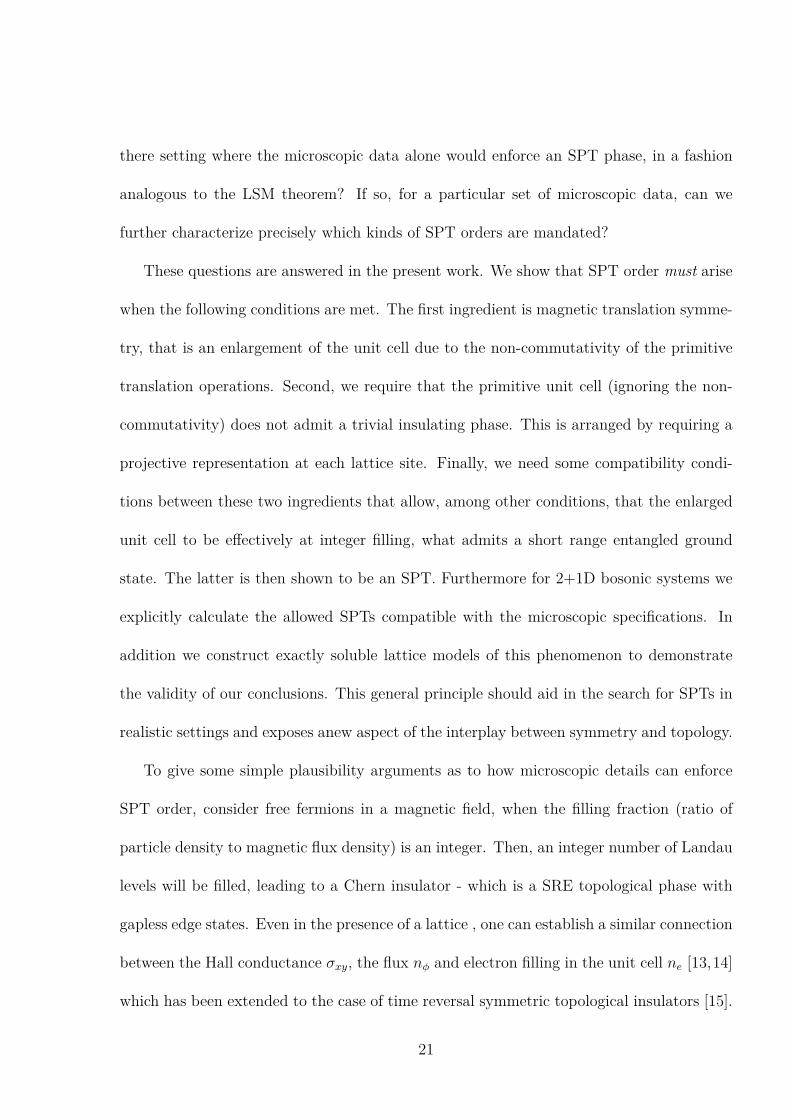
there setting where the microscopic data alone would enforce an SPT phase, in a fashion
analogous to the LSM theorem? If so, for a particular set of microscopic data, can we
further characterize precisely which kinds of SPT orders are mandated?
These questions are answered in the present work. We show that SPT order must arise
when the following conditions are met. The first ingredient is magnetic translation symme-
try, that is an enlargement of the unit cell due to the non-commutativity of the primitive
translation operations. Second, we require that the primitive unit cell (ignoring the non-
commutativity) does not admit a trivial insulating phase. This is arranged by requiring a
projective representation at each lattice site. Finally, we need some compatibility condi-
tions between these two ingredients that allow, among other conditions, that the enlarged
unit cell to be effectively at integer filling, what admits a short range entangled ground
state. The latter is then shown to be an SPT. Furthermore for 2+1D bosonic systems we
explicitly calculate the allowed SPTs compatible with the microscopic specifications. In
addition we construct exactly soluble lattice models of this phenomenon to demonstrate
the validity of our conclusions. This general principle should aid in the search for SPTs in
realistic settings and exposes anew aspect of the interplay between symmetry and topology.
To give some simple plausibility arguments as to how microscopic details can enforce
SPT order, consider free fermions in a magnetic field, when the filling fraction (ratio of
particle density to magnetic flux density) is an integer. Then, an integer number of Landau
levels will be filled, leading to a Chern insulator - which is a SRE topological phase with
gapless edge states. Even in the presence of a lattice , one can establish a similar connection
between the Hall conductance σxy, the flux nϕ and electron filling in the unit cell ne [13,14]
which has been extended to the case of time reversal symmetric topological insulators [15].
21

To state our result more precisely, we consider a two dimensional lattice where the unit
translations obey: TxTyT−1x T−1
y = g, where g is an element of the symmetry group G. This
generalizes the notion of a magnetic translation, particles acquire a phase factor depending
on their g charge. We assume g is in the center of the symmetry group G (i.e. commutes
with all other elements), but otherwise consider a general G, which can either be discrete
or continuous, Abelian or nonAbelian, and can include time reversal implemented by an
antiunitary representatation. Furthermore, in each unit cell a projective representation
of the symmetry group labeled by ‘α’ is present. We derive a formula which provides a
necessary and sufficient condition on these inputs to allow for a SRE phase, and determine
constraints on the resulting SPT. Physically, this formula demands that a symmetry flux g
inserted into this system will precisely generate a projective representation that can screen
‘α’ [15].
Let us give two physical pictures to view this filling and flux enforced SPTs. First
we describe a vortex condensation based picture, for a system of lattice bosons with a
conserved U(1) charge, with flux nϕ and filling nb per lattice unit cell. Although our
chapter focuses on having projective representations per site (rather than fractional filling)
this example will be useful to build intuition. It is well known that a conventional insulator
can be thought of as a condensate of vortices. However, for fractional filling nb, the vortices
see a fractional flux per unit cell [16], and their condensate will break lattice symmetries.
Similarly, the bosons themselves cannot condense without breaking lattice symmetries due
to the fractional flux nϕ. However the bound state of a vortex and p bosons may be able to
propagate freely if: nb ± pnϕ ∈ Z is an integer. The resulting object is a boson for p even
which can then condense giving rise to a SRE and symmetric insulator. These are nothing
22

but the Bosonic Integer quantum Hall insulators at ν = nb/nϕ = p [12, 17, 18]. Note, here
the condensing particle carries unit vorticity and hence the resulting insulator is free of
topological order [19] and also preserves the U(1) symmetry since the condensing charge is
attached to vorticity. A generalization of this result to include arbitrary symmetry groups
is the main result of this chapter. An interesting exception occurs for p = 1, which is
realized for example when one has bosons at half filling (or a projective representation of
U(1) o Z2), and a π flux in each unit cell. The doubled unit cell is at integer filling. At
first sight it appears we can obtain an insulator by condensing the vortex-charge composite
which sees no net flux in the unit cell. However, this composite is a fermion and cannot
be condensed. This is also seen by a flux threading argument [14] that constrains such
SRE phases to have σxy = odd integer, which is impossible for a SRE topological phase of
bosons [17,18]. Interestingly, this result continues to hold if the U(1) is broken to a discrete
symmetry as shown below.
A second perspective is to begin in a topologically ordered phase with fractionalized ex-
citations and consider confining all exotic excitations by an appropriate anyon condensate.
For example, for bosons at half filling, one could obtain toric code (Z2) topological order
where the e particle carries half charge [20]. The m particle however sees the fractional
charge density as background flux and cannot condense while preserving spatial symme-
tries. This is the situation in the absence of magnetic translations, where the LSM theorem
enforces topological order for gapped symmetric states. However, once we allow for mag-
netic translations with g charge, a way out to an SRE phase may become available. The
m particle, bound to a g charge that sees the magnetic flux, forms a composite object that
may condense uniformly and confine the topological order. At the same time, this leads
23

to an SPT phase since the condensing anyon carries nontrivial symmetry charge [21, 22].
Indeed this picture will allows us to construct models of such LSM enforced SPT phases as
we describe below.
Before discussing construction of models, it may be helpful to give a few examples.
Consider a system of degenerate doublets (“S=1/2”) on sites of a square lattice. This
site degeneracy may arise from spin rotation invariance (SO(3)), or even just as Kramers
degeneracy protected by time reversal ZT2 symmetry. Now consider an additional Z2 sym-
metry which is invoked in defining the magnetic translations, i.e. we have a fully frustrated
Ising model on the same lattice. According to our results, in both these situations SRE
ground states are possible but must be SPT phases. While the SPT phase is unique for
the second case of Kramers doublets of ZT × Z2, in the former case of SO(3) × Z2 there
is more than one SPT phase possible. Interestingly, if we consider a minor modification of
the ZT × Z2 model, such that the doublets on each site are non Kramers pairs, protected
by the combination of the two symmetries, then no SRE ground state exists (and hence no
SPT exists) that respects all symmetries. These examples are discussed in detail in Section
2.3.1 which also introduces models that realize them.
In constructing models, the first step is to begin in the deconfined phase of a discrete
lattice gauge theory (or of a dimer model). Then, one way to obtain a confined phase is by
decorating the electric field lines with domain walls of a global symmetry. This identification
implies that we have condensed the composite of magnetic flux and symmetry charge. The
resulting confined phase is potentially an SPT if the electric charges are associated with
the appropriate symmetry fractionalization [21, 22]. However, to obtain an LSM enforced
SPTs the situation is different since they involve fractional spin on the sites. In a dimer
24

model this corresponds to having an odd number of dimers associated with a unit cell, in
which case we cannot decorate them with regular domain walls (which should be closed
loops). However if the global symmetry is also associated with flux in the unit cell (for
example a fully frustrated Ising model), the two kinds of frustration cancel each other out,
and one can still achieve this decoration of electric field line. This is discussed explicitly
in Section 2.2, for a specific model and the resulting state is shown to be the desired SPT.
The model there is one of hardcore bosons on the Kagome lattice tuned to half filling by
particle hole symmetry, previously introduced by Balents Fisher and Girvin [23]. While
their focus was on a Z2 spin liquid phase, we decorate their model with an additional Z2
symmetry realized by a fully-frustrated Ising model. The combination is shown to realize
an LSM enforced SPT phase with gapless edge states, but a short range entangled bulk.
Finally in Section 2.3 we discuss the problem for general symmetry groups, and derive
the necessary and sufficient conditions for SRE phases to emerge and identify the class of
SPTs that must be realized. Proofs can be found in the appendices.
2.2 A simple model realizing SPT phase
Our discussion starts from a concrete microscopic model realizing an SPT phase. The
beauty of this model is its simplicity, which only includes two-spin and three spin interac-
tions. It turns out that the crucial features of this model can be systematically generalized
which form the main results of the current study.
The model constructed below (see Eq.(2.5)) is based on the Balents-Fisher-Girvin(BFG)
model [23]. The original BFG model [23] is a model with spin-1/2 residing on Kagome
25

;
Figure 2.1: (color online) Degrees of freedom in the decorated BFG model. The Ising d.o.f.
σI live on the honeycomb lattice and the spin d.o.f. Si lives on the Kagome lattice. The
Ising coupling signs sIJ = +1 on red bonds, and sIJ = −1 on blue bonds. The thick red
bonds represent the “y-odd zigzag chains” used in Eq. (2.14)
lattice. It is the low energy effective Hamiltonian if we take the Jz ≫ J⊥ limit of the
following XXZ Hamiltonian
HXXZ = J⊥∑7
[(∑i∈7
Sxi )
2 + (∑i∈7
Syi )
2 − 3] + Jz∑7
(∑i∈7
Szi )
2, (2.1)
which has a spin-liquid ground state for Jz ≫ J⊥ with deconfined spinons as confirmed by
various numerical methods [24, 25].
Let’s then take a look at the low energy effective Hamiltonian. The limit Jz ≫ J⊥
ensures that Sz7 = 0 for every hexagon and the resulting Hamiltonian in this low energy
manifold takes the following ring-exchange form
HBFG = −Jring∑▷◁
(∣∣ ↓ ↑
↑ ↓⟩⟨ ↑ ↓
↓ ↑∣∣+ h.c.), (2.2)
with Jring = J2⊥/Jz.
Let’s then decorate the XXZ model by putting a layer of Ising spins σ inside every
26

triangle of the Kagome lattice, which comprises a honeycomb lattice. The Ising spins are
in a transverse field, i.e.,
HIsing = h∑I
σxI , (2.3)
with Ising spin σI living on the honeycomb lattices labeled by I.
We then couple these two layers through a binding term
Hbinding = −∑
Ii
J
λSzi · (sIJσz
IσzJ), (2.4)
where the summation is over all the bonds IJ on honeycomb lattice with Si at the bond
center. The sign sIJ = ±1 are frustrated in the sense that∏
I,J∈7 sIJ = −1. We have
specifically chosen a choice of sIJ in Fig. 2.1. The binding term binds spin-up with Ising
happy bond (sIJσzIσ
zJ = +1) and spin-down with Ising un-happy bond (sIJσz
IσzJ = −1).
The full Hamiltonian we are considering is then given by (see Fig. 2.1)
H = HXXZ +Hbinding +HIsing. (2.5)
One can divide H into two parts
H0 = Jz∑7
(Sz7)2 −∑
Ii
J
λSzi (sIJσ
zIσ
zJ).
H1 = J⊥∑7
[(Sx7)2 + (Sy7)2 − 3] +∑I
hσxI .
(2.6)
Considering the the limit where Jz, λ≫ J⊥, h, we can first deal with H0 and then treat
H1 as a perturbation. All the terms in H0 commutes with each other and hence all the eigen-
states and eigen-energies are known for H0. In fact, there is a two-to-one mapping from the
ground state sector to the low energy sector of the BFG model (i.e. Szi configurations
satisfying 3 Sz = +1/2 per hexagon). We will consider periodic boundary conditions, and
27

the Hilbert space of the original BFG model has four topological sectors labeled by parities
of the∏
k∈C 2Szk around the non-contractable loops C (which is just the non-contractable
vison flux line [26]). This mapping only map onto one specific topological sector since∏k∈C 2S
zk is identified with
∏IJ∈C sIJ due to Hbinding. The preimage of any low energy
Szi configuration inside this topological sector are two states |Sz
i ,+⟩ and |Szi ,−⟩
(related to each other by a global Ising flip).
It turns out that the effective Hamiltonian in the parameter regime where Jz ≫ λ ≫
J⊥, h and h2
λ2 ≫ J⊥Jz
has the following form (see Appendix. 2.7.1 for detailed calculation)
Hdeco.BFG = −10J2⊥h
2
9Jzλ2
∑▷◁
(∣∣ ↓ ↑
↑ ↓
−σzI
−σzJ
⟩⟨ ↑ ↓
↓ ↑
σzI
σzJ
∣∣+ h.c.). (2.7)
Note that the kinetic term in this effective Hamiltonian is the ring exchange term of four
spins at the ends of each bowtie as in the original BFG model combined with the flipping
term of the two Ising d.o.f. within this bowtie, such that the constraint Szi (sIJσ
zIσ
zJ) = 1
is still satisfied everywhere.
We shall then prove that the ground state of the decorated BFG model is a symmetric
short-range entangled SPT state. In fact, using the mapping P between the Hilbert space
of the decorated BFG model and the original BFG model
P : (|Szi ,+⟩+ |Sz
i ,−⟩)/√2 → |Sz
i ⟩ . (2.8)
Such a mapping is clearly an isometry. Next we notice that
PHdeco.BFGP−1 = HBFG, (2.9)
with the identification Jring = 10J2⊥h2
9Jzλ2 , which can be proven by directly comparing the matrix
elements on the two sides.
28
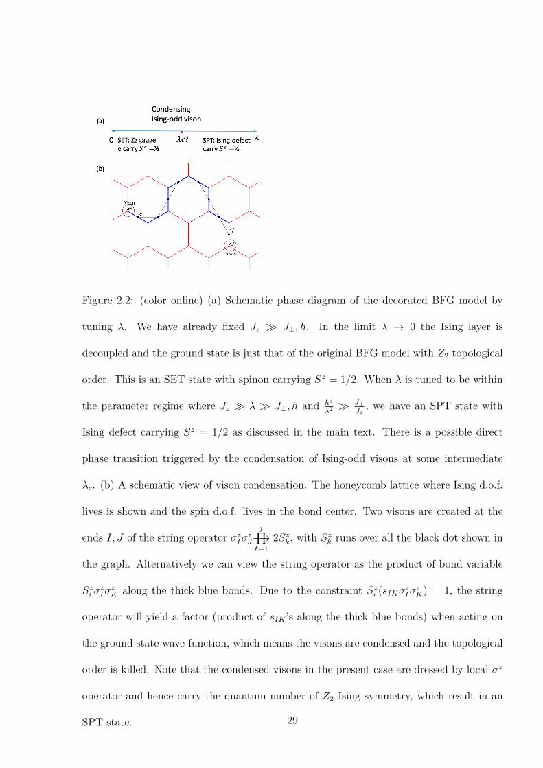
Figure 2.2: (color online) (a) Schematic phase diagram of the decorated BFG model by
tuning λ. We have already fixed Jz ≫ J⊥, h. In the limit λ → 0 the Ising layer is
decoupled and the ground state is just that of the original BFG model with Z2 topological
order. This is an SET state with spinon carrying Sz = 1/2. When λ is tuned to be within
the parameter regime where Jz ≫ λ ≫ J⊥, h and h2
λ2 ≫ J⊥Jz
, we have an SPT state with
Ising defect carrying Sz = 1/2 as discussed in the main text. There is a possible direct
phase transition triggered by the condensation of Ising-odd visons at some intermediate
λc. (b) A schematic view of vison condensation. The honeycomb lattice where Ising d.o.f.
lives is shown and the spin d.o.f. lives in the bond center. Two visons are created at the
ends I, J of the string operator σzIσ
zJ
j∏k=i
−→ 2Szk . with Sz
k runs over all the black dot shown in
the graph. Alternatively we can view the string operator as the product of bond variable
Szi σ
zIσ
zK along the thick blue bonds. Due to the constraint Sz
i (sIKσzIσ
zK) = 1, the string
operator will yield a factor (product of sIK ’s along the thick blue bonds) when acting on
the ground state wave-function, which means the visons are condensed and the topological
order is killed. Note that the condensed visons in the present case are dressed by local σz
operator and hence carry the quantum number of Z2 Ising symmetry, which result in an
SPT state. 29
Therefore the spectrum of Hdeco.BFG within the Ising-even sector is exactly the same as
that of HBFG inside a specific topological sector, which is known to be gapped. And the
ground state |ψ⟩ of HBFG, should also be mapped to the ground state |ψdeco.⟩ of Hdeco.BFG.
However there is still one possibility that there exists a state in the Ising-odd sector with
exactly the same energy as |ψdeco.⟩, which features the Ising symmetry breaking. This
possibility is ruled out because |ψdeco.⟩ has no long-range order in σz as will be discussed
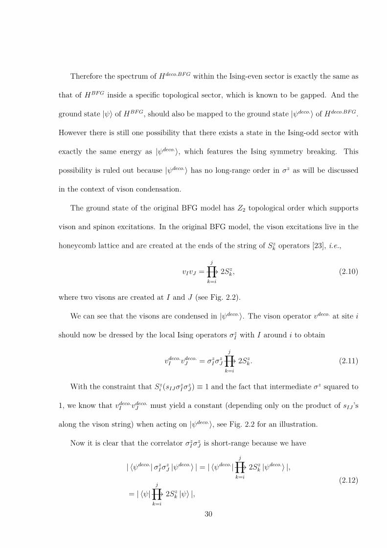
in the context of vison condensation.
The ground state of the original BFG model has Z2 topological order which supports
vison and spinon excitations. In the original BFG model, the vison excitations live in the
honeycomb lattice and are created at the ends of the string of Szk operators [23], i.e.,
vIvJ =
j∏k=i
−→ 2Szk , (2.10)
where two visons are created at I and J (see Fig. 2.2).
We can see that the visons are condensed in |ψdeco.⟩. The vison operator vdeco. at site i
should now be dressed by the local Ising operators σzI with I around i to obtain
vdeco.I vdeco.J = σzIσ
zJ
j∏k=i
−→ 2Szk . (2.11)
With the constraint that Szi (sIJσ
zIσ
zJ) ≡ 1 and the fact that intermediate σz squared to
1, we know that vdeco.I vdeco.J must yield a constant (depending only on the product of sIJ ’s
along the vison string) when acting on |ψdeco.⟩, see Fig. 2.2 for an illustration.
Now it is clear that the correlator σzIσ
zJ is short-range because we have
| ⟨ψdeco.|σzIσ
zJ |ψdeco.⟩ | = | ⟨ψdeco.|
j∏k=i
−→ 2Szk |ψdeco.⟩ |,
= | ⟨ψ|j∏
k=i
−→ 2Szk |ψ⟩ |,
(2.12)
30

where the last correlator exhibits exponential decay since visons are deconfined in the
original BFG model (the last equality holds because P commutes with the string operator).
The above discussions feature the physical picture of the condensation of visons carrying
Ising quantum number, which kills the Z2 topological order. We will soon show that the
resulting phase is an SPT phase, which is exactly a realization of the anyon condensation
mechanism to obtain SPT phases proposed in Ref. [21]. In fact, if we start from the
decoupling limit with λ = 0 and gradually increase λ with all other couplings fixed, we
should be able to see two phases: an SET phase with spinon carrying Sz = 1/2 when λ
small and an SPT phase resulting from the condensation of Ising-odd visons when λ is in
the parameter regime Jz ≫ λ≫ J⊥, h and h2
λ2 ≫ J⊥Jz
. This two phases might be related by
a continuous phase transition at some intermediate λc. See Fig. 2.2 for an illustration.
One way to see that the ground state of the decorated BFG model Eq.(2.7) is an
SPT phase is to consider the Ising defects, which turn out to be topologically bound with
Sz = ±1/2 — a projective representation of the symmetry group (see discussion below).
In order to introduce Ising defects we need to take a branch cut and modify the terms
straddling the branch cut such that only one side is conjugated by the Ising symmetry
σx. The net effect is that for the bonds IJ crossed by the branch cut, the sign of sIJ is
flipped. See Fig. 2.3 for an illustration. To compute the Sz quantum number carried by
the Ising defect it is convenient to introduce the equivalent hard-core boson description:
ni ≡ Szi + 1/2. Now let’s take a loop C enclosing one of the Ising defect and measure
the total charge within the area D bounded by C. This is done by the following U(1)
transformation ∏7∈D
(∏i∈7
eiθ2ni) =
∏i∈C
eiθ2ni ·
∏i∈D/C
eiθni , (2.13)
31

;
Figure 2.3: (color online) An pair of Ising defects (only one is shown) is created at the end
points of the branch cut (dashed black line) after modifying the original Hamiltonian H
in Eq.(2.5) into H ′. The sign sIJ is flipped in H ′ along the branch cut comparing with
the original model. (red bond: sIJ = +1, blue bond: sIJ = −1) For any loop C enclosing
the Ising defect as the gray loop shown here, the product∏sIJ around the loop flips sign
comparing with the original model. In order that H ′binding does not cost extra energy, the
spin should be flipped wherever sIJ changes its sign. As a result, the total Sz around the
loop C is changed by an odd integer. The result is that Ising defect is topologically bound
with a half-integer spin. See the discussion in the main text.
32

from which we know that the fractional charge part is determined by boson numbers on
the boundary only.
In order that the binding term after modification H ′binding does not cost energy, the
boson number ni on the bond IJ across the branch cut should be changed by 1. Since
C only crosses Ising defect line odd times, the total boson numbers around C should be
changed by 1(mod 2). From Eq. (2.13), this amounts to the change of charge within D by
12(mod 1). This fact doesn’t depend on the position of the branch cut or the position of C
we have chosen, indicating that the extra 12
charge is bounded with the Ising defect. In the
original spin language it means Ising defect carries spin Sz = ±1/2.
Summary: Before proceeding let’s pay close attention to the symmetry property of the
Hamiltonian in Eq. (2.5). This model has the following Z2g×(U(1)oZ2h) onsite symmetry
1. Spin-rotation symmetry U(1):∏i
eiθ(Szi +
12), with θ ∈ [0, 2π).
2. Spin-flip and Ising-flip symmetry Z2h = I, h:∏i
Sxi
∏I∈A
σxI , which flips all the spins
on Kagome lattice and Ising d.o.f on A sublattice of the honeycomb lattice. This
symmetry operation leaves the Hamiltonian in Eq. (2.5) invariant.
3. Ising symmetry Z2g = I, g:∏I
σxI , which flips all the Ising d.o.f. on the honeycomb
lattice.
The onsite symmetry group has the direct product structure G = Z2g×(U(1)oZ2h). In
addition, every unit cell (three kagome sites and two honeycomb sites) carries a nontrivial
projective representation of U(1)oZ2h (i.e. a half-integer spin). Naively one would suspect
that the LSM theorem would rule out a symmetric short-range-entangled state in such a
system. However, due to the frustrated nature of the gluing term, we actually have magnetic
33

translation symmetry Tx, Ty in the system instead of usual translation T orig.x , T orig.
y , which
can be written as
Tx = (∏
I∈y-odd zigzag chainsσxI )T
orig.x ,
Ty = T orig.y ,
(2.14)
which satisfy the magnetic translation algebra
TxTyT−1x T−1
y = g. (2.15)
Therefore it is still possible for us to have an SPT state. And we also know that the
g-defect carries Sz = ±1/2, which has the same projective representation as that carried
by the unit-cell. Below we will find that this is not merely a coincidence and there is
a deep connection between the patterns of short-range entanglement and the projective
representation carried by a unit-cell related by the magnetic translation algebra.
2.3 Main Results
Our main results are captured in two theorems. Theorem-I is easier to state but less general.
Theorem-II is more general but is more mathematically involved to state.
Consider a two-dimensional bosonic quantum system respecting an onsite symmetry
group G (which could contain time-reversal), and g is a unitary symmetry element in the
center of G (i.e., g commutes with any element in G). The system respects a “magnetic”
translation symmetry group generated by Tx, Ty satisfying the algebra:
TxTyT−1x T−1
y = g, (2.16)
where Tx, Ty are assumed to be the usual translation operations combined with certain site-
dependent onsite unitary transformations. We further assume that the physical degrees of
34

freedom (d.o.f.) in each real space unit cell (not the enlarged magnetic unit cell) form a
nontrivial projective representation α of G, specified by a 2-cocycle: ∀a, b ∈ G,α(a, b) ∈
U(1) and α ∈ H2(G,U(1)). Precisely, the unitary or antiunitary transformation Ua, Ub of
a, b ∈ G satisfy:
UaaUb = α(a, b)Uab, (2.17)
where the left-superscript a in aUb denotes the group action of a on Ub: if a is unitary
(antiunitary), then aUb = Ub (aUb = U∗b , i.e. complex conjugation of Ub).
We ask the following question: is it possible for such a system to have a short-range
entangled(SRE) gapped ground state without breaking symmetries?
Here we use the definition of SRE states following Ref. [12]; i.e., those are gapped
quantum phases that can be deformed into the trivial product state via local unitary
transformations. Note that if the system respects usual translational symmetries, this
would be impossible: constrained by a generalized Lieb Shultz Mattis theorem [1, 2, 4],
the nontrivial projective representation per unit cell indicates that a gapped liquid ground
state necessarily features topological order. Here because the system respects a magnetic
translation symmetry, it is possible that a SRE liquid ground state exists. We give sufficient
and necessary conditions for such a liquid phase to exist, and show that this SRE liquid
phase must be an SPT phase.
In the presence of an onsite symmetry group G, focusing on bosonic systems specified
by Eq.(2.16,2.17), we have the following theorems:
35

Theorem-I: Here we further assume that G = G1 × ZN where ZN is the finite
abelian subgroup generated by g. The quantum system above can have a SRE liquid
ground state if and only if the two conditions below are both satisfied. Such a liquid
phase is necessarily a nontrivial SPT phase because the g-symmetry defect must carry
the projective representation α.
1. αN ≃ 1 ∈ H2(G,U(1)), i.e. N of these projective representations fuse into a
regular representation.
2. The group function (which maps elements of the symmetry group to phases, while
preserving the group relations) γαg (a) ≡ α(g,a)α(a,g)
, ∀a ∈ G is a trivial 1-cocycle (or
equivalently, a trivial one-dimensional representation):
γαg ≃ 1 ∈ H1(G,U(1)).
What is the physical meaning of these two conditions? The first condition ensures that
the enlarged magnetic unit cell does not have projective representations. Interestingly, this
is not sufficient to ensure an SRE phase. Additionally, condition 2 must be satisfied, which
essentially states that the symmetry involved in magnetic translations, g, can be chosen to
commute with all other projective group actions in a proper gauge.
Theorem-II: Here we do not make extra assumptions on G. The quantum system
above can have a SRE liquid ground state if and only if there exists a 3-cocyle ω0:
∀a, b, c ∈ G,ω0(a, b, c) ∈ U(1) and ω0 ∈ H3(G,U(1)), such that the group function
δω0g (a, b) ≡ ω0(g,a,b)ω0(a,b,g)
ω0(a,g,b)is 2-cycle equivalent to α−1: δω0
g ≃ α−1 ∈ H2(G,U(1)). Such
36

a liquid phase is necessarily a nontrivial SPT phase because the g-symmetry defect
must carry the projective representation α. The possible nontrivial SPT phases form a
coset from the classification point of view (see Remark below).
Remark: it is straightforward to show that ∀α ∈ H2(G,U(1)), γαg ∈ H1(G,U(1)).
And similarly ∀ω ∈ H3(G,U(1)), δωg ∈ H2(G,U(1)). The mappings γg : H2(G,U(1)) →
H1(G,U(1)) and δg : H3(G,U(1)) → H2(G,U(1)) reducing a n-cocycle to a (n − 1)-
cocycle are the so-called slant-products in mathematical context. γg and δg preserve the
multiplication relation in the cohomology group. In particular, there is a subgroup Ag ∈
H3(G,U(1)) such that ∀ω ∈ Ag, δωg ≃ 1 ∈ H2(G,U(1)), (i.e., Ag the kernal of the mapping
δg).
When the condition in Theorem-II is satisified, ω0 must be a nontrivial element in
H3(G,U(1)) because α is nontrivial by assumption. And the realizable SPT phases form a
coset from the classification point of view. More precisely, the 3-cocyle characterizing the
SRE liquid phase must be one of the element in the following coset: ω0 · Ag.
Outline of the proof: The proof of these theorems is a combination of a pumping
argument of entanglement spectra and derivations/constructions based on a recently de-
veloped symmetric tensor-network formulation [21], which we outline here. Basically, if a
SRE liquid phase exists, by the pumping argument of entanglement spectra one knows that
the g-symmetry-defect in this phase must carry the projective representation α, and conse-
quently this phase must be an SPT phase. This physical observation can be further justified
by calculations based on symmetric tensor-networks, leading to the following mathemati-
cal result: if the 3-cocycle characterizing the SRE liquid phase as ω ∈ H3(G,U(1)), then
37

magnetic translation symmetry dictates δωg ≃ α−1, which is exactly the same mathematical
condition for the g-symmetry-defect carrying the projective representation α. In addition,
based on the symmetric tensor-network formulation, for any ω satisfying δωg ≃ α−1, a
SRE liquid phase characterized by ω respecting the magnetic translation symmetry can
be constructed. These prove that the conditions in Theorem-II are necessary and suffi-
cient for the SRE liquid phase to exist. In addition, when ω0 exists, because a 3-cocycle
ω ∈ H3(G,U(1)) satisfies δωg ≃ α−1 if and only if ω ∈ ω0 · Ag, the coset structure in the
Remark is also established.
Theorem-I is just a special case of Theorem-II. Namely when G = G1 × ZN , one can
show that if and only if the two conditions in Theorem-I is satisified does the condition in
Theorem-II is satisfied. The condition-(1) in Theorem-I is well anticipated. If condition-(1)
is not satisfied, then physical degrees of freedom form a nontrivial projective representation
of G even in the enlarged magnetic unit cell (N times larger than original unit cell), and the
generalized Lieb Shultz Mattis theorem [1,2,4] already forbids a SRE liquid phase to exist.
The condition-(2) is less obvious and more interesting, which puts additional constraints
for the existence of a SRE liquid phase (see example-(4) below).
Before going into the details of the proof, let us consider a few simple examples to see
the applications of the Theorems and the Remark.
2.3.1 Examples
In these examples, the element g in the magnetic translation algebra Eq.(2.16) generates a
ZIsing2 ≡ I, g Ising symmetry group. For instance, a fully frustrated Ising model on the
square lattice would satisfy this magnetic translation symmetry. The symmetry-enforced
38

SPT phases in example-(1,2,3) will be demonstrated via a class of decorated quantum dimer
models, which are exactly solvable at the Rokhsar-Kivelson points [27].
(1) G = SO(3)× ZIsing2 , and a spin-1/2 per unit cell: Namely, the projective
representation α per unit cell is nontrivial because only the SO(3) part is projectively
represented, and the Ising and the spin-rotation still commute: α(g, a) = α(a, g), ∀a ∈ G.
Clearly the two conditions in Theorem-I are both satisified. First, two spin-1/2’s fuse into
a regular SO(3) representation, and γαg (a) = 1,∀a ∈ G.
According to Theorem-I, at least one SRE liquid phase can exist and must be an SPT
phase in which the g-symmetry-defect carries a half-integer spin. To understand how many
SPT phases are possibly realized, one can follow the Remark. 1 The result is that among
all possible SPT phases classified by H3(SO(3) × ZIsing2 , U(1)) = Z × Z2
2 , only one of the
Z2 indices is enforced to be nontrivial. And there are many distinct SPT phases that can
be realized, which form a coset ω0 ·Ag, where Ag = Z×Z2. In particular, after gauging the
ZIsing2 symmetry, one may obtain either the toric-code or double-semion topological order,
depending on which SPT phase is realized.
(2) G = ZT2 × ZIsing
2 , and a Kramer doublet per unit cell: Here ZT2 = I, T is
the time-reversal symmetrg group. Denoting the Ising and time-reversal transformations on
the physical d.o.f. in one unit cell as Ug, and UT (antiunitary), the projective representation
1SPT phases protected by G = SO(3)× ZIsing2 form a group H3(SO(3)× ZIsing
2 , U(1)). The Kunneth
formula gives: H3(SO(3)×ZIsing2 , U(1)) = H3(SO(3), U(1))×H3(Z2, U(1))×H2(SO(3), Z2) = Z×Z2×Z2.
Following the Remark, it is straightforward to show that only the Z2 index in H2(SO(3), Z2) is enforced to
be nontrivial. (Namely ω0 in Theorem-(2) can be chosen to be the nontrivial element in H2(SO(3), Z2),and
the kernal Ag = H3(SO(3), U(1))×H2(SO(3), Z2) = Z × Z2.)
39

α per unit cell satisfies:
U2g = 1, UT U
∗T = −1, UT U
∗g = UgUT . (2.18)
For instance, this algebra is satisfied if Ug = σx and UT = iτy for a four-dimensional
local Hilbert space (upon which σ and τ Pauli matrices act). One can check that the
two conditions in Theorem-(1) are both satisfied, and thus at least an SRE liquid phase
can exist and must be an SPT phase in which the g-symmetry-defect carries the projective
representation α (a Kramer-doublet) above.
Naively this example is very similar to the example-(1). However there is an important
difference. In this example, only one SPT phase can be realized — following the Remark,
this is because the kernel subgroup Ag is the trivial Z1 group. 2 After gauging the ZIsing2
symmetry, one must obtain a toric code topological order. This realizable SPT phase is
topologically identical to the one obtained by decorating Ising domain walls with the ZT2
Haldane chains [30].
(3) G = ZT2 × ZIsing
2 , and a non-Kramer doublet per unit cell: Here the projective
representation α per unit cell satisfies:
U2g = 1, UT U
∗T = 1, UT U
∗g = −UgUT . (2.19)
For instance, Ug = σx and UT = σz on a two-dimensional local Hilbert space would satisfy
this algebra. One can check that the two conditions in Theorem-(1) are both satisfied,
2Following the Kunneth formula: H3(ZT2 × ZIsing
2 , U(1)) = H3(ZT2 , U(1)) × H3(Z2, U(1)) ×
H2(ZT2 , Z2) = Z1 × Z2 × Z2. In this example, the Z2 index in H2(ZT
2 , Z2) is enforced to be nontriv-
ial, and the Z2 index in H3(Z2, U(1)) is enforced to be trivial. This is because here ω0 in Theorem-2 is the
nontrivial element in H2(ZT2 , Z2), and the kernel subgroup Ag = Z1.
40

and thus at least an SRE liquid phase can exist and must be an SPT phase in which the
g-symmetry-defect carries the projective representation α (a Kramer-doublet) above.
Similar to example-(2), there is only one realizable SPT phase. This SPT phase turns
out to be the non-trivial Levin-Gu SPT phase protected by the ZIsing2 alone. 3 Namely,
here after gauging the ZIsing2 symmetry, one must obtain a double-semion topological order.
(4) G = Z′2 × ZIsing
2 , and a projective representation per unit cell: In this exam-
ple, Z ′2 = I, h is another unitary Ising symmetry group. The projective representation α
satisfies:
U2g = 1, U2
h = 1, UgUh = −UhUg. (2.20)
For instance, Ug = σx, Uh = σz realize this algebra. Two of such projective representations
fuse into a regular representation of G, so the condition-(1) in Theorem-(1) is satisified.
But one can show that the condition-(2) is not satisfied:
γαg (h) = −1, (2.21)
i.e., γαg is a nontrivial 1-cocycle. Therefore according to Theorem-(1), a SRE liquid phase is
not possible. Without breaking symmetry, this suggests that topological order is inevitable
for gapped systems. This is a somewhat surprising result. If one views the system using
the enlarged magnetic unit cell, there is no reason why a SRE liquid is not allowed.
3Now in this example, ω0 in Theorem-2 is the nontrivial element in H3(Z2, U(1)), and the kernel
subgroup Ag = Z1.
41

2.4 Decorated Quantum Dimer Models for SPT phases
Closely related to the decorated-BFG model in Sec.2.2, in this section we describe a class
of exactly solvable models realizing symmetry-enforced SPT phases. These models are
constructed by decorating quantum dimer models(QDM) with relevant physical degrees of
freedom, whose ground states can be exactly solved at the corresponding Rokhsar-Kivelson
point [27]. Although this class of models can be generalized to other lattices, here we will
focus on the decoration of the QDM on the triangular lattice [32, 33]. In particular, we
will construct models realizing the symmetry-enforced SPT phases in example-(1,2,3) in
Sec.2.3.1
2.4.1 G = SO(3)× ZIsing2 , a spin-1/2 per unit cell
Continuing with discussions in example-(1) in Sec.2.3.1, in the presence of onsite global
symmetry G = SO(3) × ZIsing2 , we consider quantum systems with one spin-1/2 per unit
cell in two spatial dimensions respecting the Ising magnetic translation symmetry Eq.(2.16).
Note that we will reserve symbols Tx, Ty for the magnetic translations, and use T orig.x , T orig.
y
to represent the original translations.
We will construct two exactly solvable models (model-A and model-B) respecting the
symmetry described above featuring SRE liquid ground states. Although the Ising defects
in both models carry half-integer spins, the two models are in distinct SPT phases. The
simplest way to understand their difference is that, after gauging the Ising symmetry, model-
A has toric-code topological order while model-B has double-semion topological order.
We start with constructing model-A. This model contains two sets of degrees of freedom
(d.o.f.): the Ising-d.o.f. σI which live on a honeycomb lattice and the spin-1/2-d.o.f. Si =
42

Tx
Ty
σIσJ
τj
τi
Figure 2.4: (color online) The Ising d.o.f. σ live on the honeycomb lattice and the spin
d.o.f. τ lives on the triangular lattice. The Ising coupling signs sIJ = +1 on red bonds,
and sIJ = −1 on blue vertical bonds. The thick red bonds represent the “y-odd zigzag
chains” used in Eq.(2.25,2.36 ). The thick gray horizontal bonds on the triangular lattice
represent the “y-odd rows” used in Eq.(2.36).
43
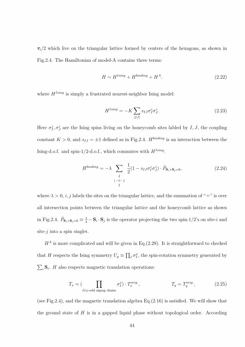
τi/2 which live on the triangular lattice formed by centers of the hexagons, as shown in
Fig.2.4. The Hamiltonian of model-A contains three terms:
H = HIsing +Hbinding +HA. (2.22)
where HIsing is simply a frustrated nearest-neighbor Ising model:
HIsing = −K∑⟨IJ⟩
sIJσzIσ
zJ . (2.23)
Here σzI , σ
zJ are the Ising spins living on the honeycomb sites labled by I, J , the coupling
constant K > 0, and sIJ = ±1 defined as in Fig.2.4. Hbinding is an interaction between the
Ising-d.o.f. and spin-1/2-d.o.f., which commutes with HIsing:
Hbinding = −λ∑
i jI
J
1
2(1− sIJσ
zIσ
zJ) · PSi+Sj=0, (2.24)
where λ > 0, i, j labels the sites on the triangular lattice, and the summation of “ ” is over
all intersection points between the triangular lattice and the honeycomb lattice as shown
in Fig.2.4. PSi+Sj=0 ≡ 14−Si ·Sj is the operator projecting the two spin-1/2’s on site-i and
site-j into a spin singlet.
HA is more complicated and will be given in Eq.(2.29). It is straightforward to checked
that H respects the Ising symmetry Ug ≡∏
I σxI , the spin-rotation symmetry generated by∑
i Si. H also respects magnetic translation operations:
Tx = (∏
I∈y-odd zigzag chainsσxI ) · T orig.
x , Ty = T orig.y , (2.25)
(see Fig.2.4), and the magnetic translation algebra Eq.(2.16) is satisfied. We will show that
the ground state of H is in a gapped liquid phase without topological order. According
44

to our general results, this ground state must be in an SPT phase, which we will show
momentarily.
The physical consequence of HIsing and Hbinding is to provide a highly degenerate low
energy manifold, which will be lifted by HA. To understand the low energy manifold,
let us firstly consider HIsing. Because every hexagonal plaquette frustrated, there will be
at least one bond in each plaquette that is energetically unhappy. Namely the ground
state manifold of HIsing is formed by all possible Ising configurations satisfying the “one-
unhappy-Ising-bond-per-plaquette” condition.
Hbinding further constrains the spin-1/2 d.o.f. in the low energy manifold. It has effect
only on the Ising unhappy bonds (sIJσzIσ
zJ = −1), and energetically binds the two spin-1/2’s
near the unhappy Ising-bond into a spin singlet. The degenerate ground state manifold of
HIsing +Hbinding is now clear: it is formed by all such quantum states satisfying the “one-
unhappy-Ising-bond-per-plaquette” condition and the two neighboring spin-1/2’s normal
to every unhappy Ising-bond form a spin singlet.
It is well-known that the Ising configurations satisfying the “one-unhappy-Ising-bond-
per-plaquette” condition are intimately related to the Hilbert space of the QDM [34–36].
Pictorically, any such an Ising configuration can be mapped to a dimer covering (with one
dimer per site) on the triangular lattice by assigning a dimer crossing the unhappy Ising
bond. The effect of Hbinding is simply to energetically binds the two spin-1/2’s in each
dimer into a spin-singlet. Namely if the Ising configuration is given, the state of spin-1/2
d.o.f. is also fixed.
Similar to the model in Sec.2.2, there is a two-to-one mapping from the ground state
manifold of HIsing +Hbinding to the QDM Hilbert space, since two low energy states differ
45
by a global Ising transformation map into the same state in the QDM. Second, these states
only map to one specific topological sector of the QDM: The parity of the number of dimers
crossing a loop is simply given by the sign of the product∏
⟨IJ⟩∈loop sIJ .
In fact, these relations between the Ising d.o.f. and the dimer d.o.f. can be viewed as
the well-known duality mapping between quantum Ising models and Z2 gauge theories [37].
The Ising paramagnet phase is dual to the deconfined Z2 gauge phase in the QDM, while the
Ising ordered phase is dual to the confined Z2 gauge theory. More precisely, the “unhappy-
Ising-bond” is dual to the electric flux line (i.e., the dimer) in the gauge theory, and the
“one-unhappy-Ising-bond-per-plaquette” condition in the low energy manifold on the Ising
side is dual to the “one-Z2-gauge-charge-per-site” condition in the QDM. Here, the only
new ingredient apart from this well-known duality is that there are also spin-1/2 d.o.f. on
the Ising side. But due to Hbinding, these spin-1/2’s form a pattern of spin singlets fixed by
the Ising d.o.f., and consequently the duality mapping is not modified after a convention
of the spin-singlet signs is given (see below).
After introducing HA, we will see that the degeneracy in the low energy manifold will
be lifted and the unique ground state on a torus sample is formed. The usual QDM
Hamiltonian on the triangular lattice is:
HTCQDM = −t
∑plaquettes
(| ⟩⟨ |+ h.c.
)+ v
∑plaquettes
(| ⟩⟨ |+ | ⟩⟨ |
), (2.26)
where the summation is over all plaquettes (rhombi): “ ”, “ ”, “ ”. The ground states of
this model are exactly known at the RK-point given by t = v > 0, and the superscript TC
is highlighting that the topological order is toric-code [32, 38] like in the deconfined phase
46

(i.e., the usual Z2 gauge theory). At this point HTCRK can be rewritten as a summation of
projectors [32]:
HTCRK = t
∑plaquettes
(| ⟩ − | ⟩
)(⟨ | − ⟨ |
). (2.27)
Clearly the equal weight superposition of all dimer coverings within any fixed topological
sector |ΦTCRK⟩ =
∑c |c⟩ (c labels possible dimer coverings) is one ground state of HTC
RK since
it is annihilated by all projectors.
Based on the duality mapping, HTCQDM is mapped to HA. Any dimer covering |c⟩ will
be mapped to two Ising configurations |c1⟩ and |c2⟩ distinct from each other by a global
Ising transformation. One can further choose a translationally symmetric sign convention
for the spin-singlets on the nearest neighbor bonds along the three orientations:
| ⟩ ≡ 1√2
(|↑↑↑ ↓↓↓⟩ − |↓↓↓ ↑↑↑⟩
),
| ⟩ ≡ 1√2
(∣∣↑↑↑
↓↓↓ ⟩−∣∣
↓↓↓↑↑↑ ⟩)
,
| ⟩ ≡ 1√2
(∣∣ ↑↑↑↓↓↓
⟩−∣∣ ↓↓↓↑↑↑
⟩)⟩. (2.28)
With this sign convention, given a c, |ci⟩ (i = 1 or 2) fully determines a state in the ground
state manifold of HIsing+Hbinding by replacing the dimer configuration by the corresponding
spin-singlet configuration. In addition, |c1⟩, |c2⟩ for all c form a complete orthornormal
basis in this manifold.
47

HA is defined as:
HA =− t
σzI ,σ
zJ=±1∑
plaquettes
(∣∣ −σzI
−σzJ⟩⟨
σzI
σzJ∣∣+ h.c.
)
+ v
σzI ,σ
zJ=±1∑
plaquettes
(∣∣ σzI
σzJ⟩⟨
σzI
σzJ∣∣
+∣∣ σz
I
σzJ⟩⟨
σzI
σzJ∣∣) (2.29)
Note that the t-term also flips the two Ising spins inside the plaquette. At the RK point
t = v > 0, HA can again be written as a summation of projectors:
HARK = t
σzI ,σ
zJ=±1∑
plaquettes
(∣∣ −σzI
−σzJ⟩−∣∣ σz
I
σzJ⟩)
·
(⟨−σz
I
−σzJ∣∣− ⟨ σz
I
σzJ∣∣) (2.30)
To study the ground state of the total Hamiltonian H, it is suffice to focus on the degenerate
ground state manifold of HIsing + Hbinding, and clearly HA acts within this manifold. In
addition, it is straightforward to show that |ΦARK⟩ =
∑c(|c1⟩ + |c2⟩), i.e, the equal weight
superposition of all states in this manifold, is a ground state of HARK because it is annihilated
by every projector in Eq.(2.30). |ΦARK⟩ is clearly a fully symmetric liquid wavefunction.
It is known that for the QDM Eq.(2.26), the RK point of H is exactly at a first-
order phase transition boundary between a deconfined gapped liquid phase (v < t) and a
staggered valence bond solid phase (v > t) [32]. Based on the duality mapping, the model-
A is in a fully symmetric gapped liquid phase for vc < v < t with a unique ground state on
torus. In the limit of K,λ ≫ v, t, vc is given by the same critical value vc ≈ 0.7t as in the
original QDM [32]. More precisely, in the global Ising-even sector of the Hilbert space of
model-A, this mapping to the Hilbert space of the QDM is given by 1/√2(|c1⟩+ |c2⟩) → |c⟩,
and clearly HA is mapped to HTCQDM . Namely, the full energy spectrum of model-A in the
48

Ising-even sector has a one-to-one correspondence with the full energy spectrum of HTCQDM .
In addition, in the Ising paramagnetic phase, ground state in the global Ising-odd sector of
model-A has a finite excitation energy which is the same as the energy cost of a Z2 gauge
flux in the QDM.
Next we show that the liquid phase vc < v < t in model-A is an SPT phase because
the Ising defects carry half-integer spins. Similar to the discussion in Sec.2.2 (see Fig.2.3),
after a pair of Ising defects are spatially separated the original Hamiltonian H is modified
into H ′. Comparing with H, the sIJ flips sign in H ′ whenever the bond I − J crosses the
branch cut. Namely, for any loop on the honeycomb lattice enclosing a single Ising defect,
the product∏sIJ along the loop changes sign. In order not to cost H ′binding energy, the
parity of the number of dimers crossing this loop also flips. Consequently, an Ising defect
is topologically bound with a monomer (an unpaired site on the triangular lattice). This
monomer clearly carries a half-integer spin in model-A, which can be detected by the local
spin susceptibility at low temperatures.
Next, we demonstrate a different symmetry-enforced SPT phase using the model-B
defined as follows:
H = HIsing +Hbinding +HB. (2.31)
Comparing with the model-A in Eq.(2.22), only the last term is modified:
HB =v
σzI ,σ
zJ=±1∑
plaquettes
(∣∣ σzI
σzJ⟩⟨
σzI
σzJ∣∣+ ∣∣ σz
I
σzJ⟩⟨
σzI
σzJ∣∣)+
σzI ,σ
zJ=±1∑ (
−it∣∣ −σz
I
−σzJ⟩⟨
σzI
σzJ∣∣+ h.c.
)
+
σzI ,σ
zJ=±1∑ (
−it∣∣ −σz
I
−σzJ
⟩⟨σzI
σzJ
∣∣+ h.c.
)+
σzI ,σ
zJ=±1∑ −it
∣∣ −σzI
−σzJ
⟩⟨ σzI
σzJ
∣∣+ h.c.
(2.32)
49

One can straightforwardly check that the model-B defined in Eq.(2.31,2.32) also respects the
Ising symmetry, the SO(3) spin-rotation symmetry, and the magnetic translation symmetry
Eq.(2.16). Below we show that in a finite parameter regime v′c < v < t, the model-B is in
a gapped liquid phase, and this phase is another SPT phase.
In the ground state manifold of HIsing +Hbinding, the duality transformation maps HB
into the following QDM Hamiltonian:
HDSQDM = v
∑plaquettes
(| ⟩⟨ |+ | ⟩⟨ |
)+∑, ,
−it(| ⟩⟨ |+ | ⟩⟨ |+ | ⟩⟨ |
)+ h.c. (2.33)
This QDM was firstly introduced and studied in Ref. [33], where the exactly solvable RK
point t = v has been shown to be adjacent a gapped liquid phase for v ≲ t. Interestingly,
this phase was demonstrated to have a double-semion topological order (the superscript DS
here is to highlight this fact). By the duality mapping, we know that in a finite parameter
regime v′c < v < t, the model-B is in a gapped liquid phase.
Similar to previous disussion on the model-A, it is straightforward to show that the
Ising defect in the gapped liquid phase of model-B also carries half-integer spin, so it is
also an SPT phase. To see the difference from the SPT phase realized in model-A, let us
consider the Ising symmetry only. It is known that Ising symmetry itself can protect two
paramagetic phases: the trivial phase and the SPT phase. Levin and Gu pointed out [39]
that the duality mapping maps the usual Ising paramagnet to the toric-code topological
order, while the nontrivial Ising SPT phase maps to the double semion topological order.
Consequently, the SPT phases realized in model-A and model-B are different because the
Ising symmetry alone already distinguishes them.
50

2.4.2 G = ZT2 × ZIsing
2
Here we demonstrate symmetry-enforced SPT phases outlined in example-(2) and (3) in
Sec.2.3.1. Unlike the G = SO(3) × ZIsing2 case, here we show that symmetry conditions
fully determine the SPT phase. The models below have the same Hilbert space as in the
G = SO(3)×ZIsing2 case (i.e., σI on the honeycomb lattice and τi on the triangular lattice),
but with different symmetries defined.
A Kramer doublet per unit cell: A simple generalization is for example-(2) (i.e.,
a Kramer-doublet per unit cell) where we can recycle the model-A. Namely, defining the
Ising symmetry Ug =∏
I σxI as before and the antiunitary time-reversal symmetry as UT =
eiπSy= iτ y, clearly model-A respect all the required symmetries. In addition, we have
one Kramer doublet τ per unit cell. According to our discussion in example-(2), this SRE
liquid phase realized in vc < v < t must be an SPT phase in which the Ising defect carries
a Kramer doublet, which is obviously realized in model-A. In addition, after gauging ZIsing2
symmetry, one necessarily obtains the toric-code topological order, which is confirmed in
model-A.
On the other hand, model-B, gauging which gives double-semion topological order,
explicitly breaks the time-reversal symmetry defined above.
A non-Kramer doublet per unit cell: Now let us move on to example-(3) in
Sec.2.3.1. In order to construct a model realizing the non-Kramer doublet projective rep-
resentation defined in Eq.(2.19), let us define the following symmetry operations:
Ug = τ z∏I
σxI , UT = τ x. (2.34)
Consequently we have one non-Kramer doublet τ per unit cell. The model Hamiltonian in
51

this example will be given by
H = HIsing + Hbinding + HB, (2.35)
where HIsing is given in Eq.(2.23), Hbinding is in Eq.(2.39). HB has the same form as HB in
Eq.(2.32), but with a modified interpretations of the dimers: replacing the | ⟩’s defined
in Eq.(2.28) by | ⟩’s and | ⟩’s defined in Eq.(2.37,2.38) depending the dimer positions
(see discussions below and Fig.2.5). Eventually we will show that in a finite regime v ≲ t
this model features a SRE gapped liquid ground state which is the Levin-Gu Ising SPT
phase, consistent with discussions in Sec.2.3.1.
We will construct a model similar toH = HIsing+Hbinding+..., but respecting a magnetic
translation operations different from Eq.(2.25) since Ug is now different. In particular, we
define magnetic translations:
Tx =( ∏i∈y-odd row
τ zi
)( ∏I∈y-odd zigzag chains
σxI
)T orig.x ,
Ty = T orig.y , (2.36)
(see Fig.2.4), which satisifies Eq.(2.16) with g =∏
i τzi
∏I σ
xI following Eq.(2.34). Although
HIsing still respects all the symmetries, Hbinding does not respect g and Tx. This is because
the usual spin singlets | ⟩ in the projector PSi+Sj=0 = | ⟩⟨ | does not respect g and
Tx. We therefore need to modify these dimer states and the projectors.
We define the following dimer states formed by the τ spins:
| ⟩ ≡ 1√2
(|↑↑↑ ↑↑↑⟩+ |↓↓↓ ↓↓↓⟩
),
| ⟩ ≡ 1√2
(∣∣↑↑↑
↑↑↑ ⟩+∣∣
↓↓↓↓↓↓ ⟩)
,
| ⟩ ≡ 1√2
(∣∣ ↑↑↑↑↑↑
⟩+∣∣ ↓↓↓↓↓↓
⟩)⟩. (2.37)
52

Figure 2.5: To construct model in Eq.(2.35), the dimer states living on the nearest neighbor
bonds on the triangular lattice have a spatial dependent pattern: the dimer states living
on the dashed bonds are defined in Eq.(2.37), and those living on the dotted bonds are
defined in Eq.(2.38).
Clearly these dimer states are both Ising and time-reversal even according to Eq.(2.34).
Under the magnetic translation Tx in Eq.(2.36), dimer states with | ⟩ and | ⟩
connecting even and odd rows on the triangular lattice will transform into the following
states:
| ⟩ ≡ 1√2
(∣∣↑↑↑
↑↑↑ ⟩−∣∣
↓↓↓↓↓↓ ⟩)
,
| ⟩ ≡ 1√2
(∣∣ ↑↑↑↑↑↑
⟩−∣∣ ↓↓↓↓↓↓
⟩)⟩. (2.38)
Note that these dotted dimer states are Ising even, but time-reversal odd according to
Eq.(2.34). The magnetic translational symmetric assignment of the dimer states is given in
Fig.(2.5): the states | ⟩, | ⟩, | ⟩ are assigned on the dashed bonds, while the states
| ⟩, | ⟩ are assigned on the dotted bonds.
By replacing the spin singlets in PSi+Sj=0 = | ⟩⟨ | by the corresponding | ⟩⟨ |
53

and | ⟩⟨ | in the spatial dependent fashion in Fig.2.5, we modify Hbinding naturally as
Hbinding = −λ∑
i jI
J
1
2(1− sIJσ
zIσ
zJ) ·
(| ⟩⟨ |
)
− λ∑
i jI
J
1
2(1− sIJσ
zIσ
zJ) ·
(| ⟩⟨ |
), (2.39)
Now HIsing+ Hbinding respects all the required symmetries, but one still need terms like
HA or HB to lift the ground state degeneracy to reach a SRE gapped liquid phase. In order
to preserve the Ising and magnetic translation symmetry, it is natural to replace the dimer
states | ⟩ by the corresponding | ⟩ and | ⟩. Let us denote the resulting modified
Hamiltonians as HA or HB. Both modified models HIsing + Hbinding + HA and HIsing +
Hbinding + HB are solvable, by duality mapping to the HTCQDM and HDS
QDM respectively.
These two models both give SRE gapped ground states in the regime v ≲ t respecting the
magnetic translation symmetry and the Ising symmetry, gauging which give toric-code and
double semion topological order respectively.
Finally, let us consider the time-reversal symmetry in Eq.(2.19). Importantly, | ⟩’s are
time-reversal even while | ⟩ are time-reversal odd. As shown in the pattern Fig.2.5, any
dimer resonant term like | ⟩⟨ | will involve an odd number of | ⟩ states. Consequently,
only HB is time-reversal symmetric, while HA explicitly breaks the time-reversal. In fact
according to Theorem-I, it is impossible to have a SRE liquid respecting all the required
symmetries and gauging the Ising symmetry gives a toric code topological order.
54

2.5 Proof of Theorems
Here we present a combination of physical argument and mathematical derivations based
on symmetric tensor network formulation [21,40–47]. We will focus on Theorem-II, and in
Appendix2.7.2 we show that Theorem-I can be viewed as its special case.
We need to show the condition in Theorem-II is necessary and sufficient for a SRE
liquid phase to exist, which must be an SPT phase. To show this condition is necessary,
we consider such a SRE liquid phase and the pumping of the entanglement spectra during
an adiabatic process in Sec.2.5.1, leading to an observation that a g-symmetry defect must
carry a projective representation α. In a SRE liquid phase characterized by 3-cocycle ω, we
use the symmetric tensor-network formulation in Sec.2.5.2 to establish that the projective
representation carried by a g-symmetry defect is given by (δωg )−1. Since the projective
representation carried by a symmetry defect is physical and independent of formulation,
together with the pumping argument, the necessary condition in Theorem-II is established
independent of formulation.
As a complementary calculation, we also explicitly compute the projective representa-
tion carried by a g-symmetry defect in a SRE liquid phase representable within the sym-
metry tensor-network formulation in Appendix.2.7.5, which turns out to be α, consistent
with the previous discussion [48].
To further show that the condition is also sufficient, we will show that for any 3-cocycle
ω0 satisfying (δω0g )−1 ≃ α, generic symmetric tensor network wavefunctions representing a
SRE liquid phase characterized by ω0 can be constructed in Sec.2.5.3.
55

2.5.1 Entanglement Pumping argument
Here let us assume a SRE liquid phase exist. It is straightforward to show that after a local
unitary transformation (a site dependent Ug action) without changing the physical action
of G, one can always choose a gauge in which Ty = T orig.y and Tx = (
∏y−odd Ug) · T orig.
x .
Then we consider putting this SRE liquid on a infinite cylinder C along the x-direction,
with Ly number of unit cells across the y-direction loop. We choose Ly = ly ·N + dy where
ly, dy are integers, gN = I and 0 ≤ dy < N . Note that if dy = 0 this choice of Ly will
explicitly break the Tx symmetry.
This infinite long cylinder can be viewed as a one-dimensional system, and for a large
enough Ly the onsite symmetry G will be respected. We will study the entanglement
spectrum of this one dimensional system at a particular cut x0 + 1/2. A SRE liquid
respecting G symmetry dictates that entanglement states at this cut carry a particular
projective representation ξ of G [49, 50].
Next, we adiabatically create a g-symmetry defect/anti-defect pair at a given y-coordinate
and separate them to infinity along the x-direction. After repeating this procedure for every
y-coordinate, we totally move Ly number of g-symmetry defects acrosses the entanglement
cut x0+1/2. As shown in Fig.2.6, the final Hamiltonian is related with the original Hamil-
tonian by the original translation operation T orig.x . Therefore, the final entanglement states
at the cut x0+1/2 is equivalent to the initial entanglement states at a different cut: x0−1/2.
Because the initial entanglement states at x0−1/2 differs from the initial entanglement
states at x0 + 1/2 by a column of unit cells along y-direction, we conclude that the final
entanglement eigenstates at x0 +1/2 must carry the αdy · ξ projective representation. This
pumping of the entanglement projective representation can only be explained by the pro-
56

x0+1/2
Figure 2.6: Illustration of adiabatically separating a pair of g-defect/antidefect along the x-
direction with g3 = I. For simplicity, one may imagine Hamiltonian to host nearest neighbor
(NN) terms. Along the x-direction, due to the magnetic translation symmetry Eq.(2.16),
the NN interactions on the vertical bonds have a three-unit-cell periodicity (solid,dashed
and dotted bonds). While the g-defect crosses the entanglement cut at x0 + 1/2, the
Hamiltonian along the branch cut (dashed gray line) is effectively translated along x-
direction by one unit cell. After separating such pairs of defects for every row, the final
Hamiltonian is related to the original Hamiltonian by T orig.x .
57
jective representation α carried by a g-symmetry defect, and (α)Ly ≃ αdy . But because N
g-defect fuse into a trivial object, we must have (α)N ≃ 1. Consequently α = α.
2.5.2 Symmetry-enforced constraints on SPT cocycles
Here we consider an SPT wavefunction represented using the symmetric tensor-network for-
mulation [21]. The advantage of this formulation is that it allows us to introduce symmetry
defects conveniently.
The local symmetry transformation of an onsite symmetry a on a g-defect is given by the
application of of Ua inside a disk D covering the g-defect, together with an application of
unitary operations on the virtual degrees of freedom on the boundary of D. This boundary
operation should be defined in such a way that after these two operations, no excitation is
created near the boundary of D. In Appendix 2.7.4 we explictly constructed such bound-
ary operations. With these boundary operations, we explicitly show that the projective
representaion carried by the g-defect is given by (δωg )−1 in an SPT phase characterized by
the 3-cocycle ω, which is given without proof in Ref. [48].
2.5.3 Generic constructions of Symmetry-enforced SPT wave-
functions
Our strategy here is to start from an SPT state characterized by a 3-cocycle ω with a regular
representation of G per unit cell and respecting the usual translation symmetry T orig.x , T orig.
y .
Such a state can be generically represented using the symmetric tensor-network formula-
tion [21]. In particular, the symmetric tensor-network needs to satisfy a collection of
algebraic equations (constraints). Then we show that after properly modifying these alge-
58

braic constraints, the new tensor-network will respect the magnetic translation symmetry
Tx, Ty, at the same time the physical d.o.f. must carry a projective representation (δωg )−1
per unit cell (otherwise the wavefunction vanishes). The tensor-network states satisfying
these modified constraints are generic constructions of the SPT states in Theorem-II.
The details of the construction can be found in Appendix 2.7.6.
2.6 Discussion
Generalized Hastings-Oshikawa-Lieb-Schultz-Mattis theorems put strong constraints on
possible symmetric quantum states of matter. In particular, in the presence of transla-
tion symmetry and a projective representation of the onsite symmetry group per unit cell,
it is impossible to have a gapped short-range entangled (SRE) symmetric ground state.
In this chapter we discuss that in the presence of magnetic translation symmetry, gapped
SRE symmetric ground states could exist, which are enforced to be symmetry protected
topological (SPT) phases. Focusing on bosonic systems in two spatial dimensions, we pro-
vide the generic necessary and sufficient condition for such symmetry-enforced SPT phases
to occur in Theorem-I and II. When the condition is satisified, we sharply characterize the
coset structure of the realizable SPT phases in the Remark.
The condition-(2) in Theorem-I is particular non-obvious. It states that if symmetries
protecting the fractional spin (projective representation) per unit cell and those generating
the magnetic translations fail to commute with one another, then SRE liquid state is
impossible even if the fractional spins fuse into an integer spin (regular representation) in
the magnetic unit cell.
59
In addition, we design a class of decorated quantum dimer models realizing some of
these symmetry-enforced SPT phases, which are exactly solvable at the corresponding
Rokhsar-Kivelson points. A particularly simple model realizing a symmetry-enforced SPT
phase is given in Sec.2.2 by coupling a Balents-Fisher-Girvin spin liquid with a layer of
pure-transverse-field Ising spins via three-spin interactions. This model also demonstrates
the route to obtain SPT phases via condensing anyons in SET phases [21, 22].
It is interesting to consider the situation of fermions with magnetic translation symme-
tries, in which case (generalized) Hastings-Oshikawa-Lieb-Schultz-Mattis theorem apply for
fractional filled systems with regular translation symmetries. In fact, earlier works [13, 14]
establish the magnetic translation symmetry protected integer Hall conductivity, and a
recent work by Wu et.al. studied the magnetic translation enforced quantum spin Hall
insulators in fractionally filled fermionic systems [15]. Connecting with these works, the
present work focuses on bosonic systems with projective representation per unit cell, but
obtains systematic results.
60

2.7 Appendices
2.7.1 Perturbation study of the decorated Balents-Fisher-Girvin
model
The Hamiltonian for the decorated BFG model can be split into two parts
Hdeco.BFG = H0 +H1,
H0 = Jz∑7
(Sz7)2 −∑
Ii
J
λSzi (sIJσ
zIσ
zJ),
H1 = J⊥∑(i,j)
S+i S
−j +
∑I
hσxI ,
(2.40)
where (i, j) runs over first, second, third neighbors within a hexagon of Kagome plaquette.
Let’s take the limit Jz, λ ≫ J⊥, h and only focus on the low energy Hamiltonian in
the ground state manifold of H0. Then we can treat H1 as a small perturbation and use
the conventional Brillouin-Wigner perturbation to derive the effective Hamiltonian. The
effective Hamiltonian is then given by (take E0 as the ground state energy of H0),
Heff = E0 + Pg(H1 +H1G′0H1 +H1G
′0H1G
′0H1 + · · · )Pg, (2.41)
where G′0 = Pe(E0 − H0)
−1Pe and Pg/Pe are the projector onto the the ground/excited
states of H0.
We will work under the limit Jz ≫ λ and calculate the effective Hamiltonian order by
order to find the leading non-constant terms in J⊥ and h since we have not specified the
relation between them yet. Let’s denote N as the number of Kagome unit-cell. The zeroth
order energy is E0 = −32Nλ. Higher order terms are as follows:
1. H(1)eff = PgH1Pg = 0.
61

2. H(2)eff = PgH1G
′0H1Pg = −9N
J2⊥
2Jz+2λ−2N · h2
3λ. The first term comes from the process of
switching a pair of spin-up and spin-down and then switching back within a hexagon.
The second term comes from the process of flipping a Ising d.o.f. twice. To this order,
we only have constant terms.
3. H(3)eff = PgH1G
′0H1G
′0H1Pg =
J3⊥
(2Jz+2λ)2
∑(i,j,k)
(S+i S
−k S
+k S
−j S
+j S
−i + S+
j S−k S
+i S
−j S
+k S
−i ),
where the summation runs over all ordered triplets (i, j, k) with (i, j), (j, k), (k, i)
appearing in H1. The term S+i S
−k S
+k S
−j S
+j S
−i = (1/2 + Sz
i )(1/2 − Szj )(1/2 − Sz
k)
measures the energy of the configuration with Szi = 1/2, Sz
j = −1/2, Szk = −1/2.
And the term S+j S
−k S
+i S
−j S
+k S
−i = (1/2 + Sz
i )(1/2 + Szj )(1/2 − Sz
k) measures the
energy of the configuration with Szi = 1/2, Sz
j = 1/2, Szk = −1/2. To this order, the
term does depend on the spin configuration and is the leading non-constant term in
J⊥.
4. H(4)eff = PgH1G
′0H1G
′0H1G
′0H1Pg = −10J2
⊥h2
9Jzλ2
∑▷◁
(∣∣ ↓ ↑
↑ ↓
−σzI
−σzJ
⟩⟨ ↑ ↓
↓ ↑
σzI
σzJ
∣∣+ h.c.) +O(h4
λ3 ) +
O(J2⊥h2
Jzλ2 ) + O(J4⊥J3z), where we have used the limit Jz ≫ λ. The first term is a kinetic
term which is the leading non-constant contribution in h. The latter three terms
are not written out explicitly due to the following reason. Terms proportional to
J4⊥J3z
are less significant compared to that from the 3-rd order perturbation. Terms
proportional to h4
λ3 (process of flipping two different Ising d.o.f. twice) is a constant.
And the potential term proportional to J2⊥h2
Jzλ2 (process of separately flipping Ising d.o.f
twice and exchanging spin-up and down twice) is also a constant in the limit Jz ≫ λ.
The leading non-constant terms are terms of order J3⊥J2z
and terms of order J2⊥h2
Jzλ2 , where
the latter is what we want. So we further require h2
λ2 ≫ J⊥Jz
such that the term obtained
62

from the 3rd-order perturbation can be neglected.
Then we achieve the decorated BFG model
Heff = −10J2⊥h
2
9Jzλ2
∑▷◁
(∣∣ ↓ ↑
↑ ↓
−σzI
−σzJ
⟩⟨ ↑ ↓
↓ ↑
σzI
σzJ
∣∣+ h.c.) (2.42)
in the parameter regime where Jz ≫ λ≫ J⊥, h and h2
λ2 ≫ J⊥Jz
.
2.7.2 Theorem-I as a special case of Theorem-II
Necessary condition for the existence of SRE state: constraints on the on-
site projective representation First we prove that only when the on-site projective
representation α satisfies the following 2 conditions is a SRE ground state possible.
1. αN ≃ 1 ∈ H2(G,U(1)).
2. γαg (a) ≃ 1 ∈ H1(G,U(1)).
Suppose the unit-cell is enlarged along x-direction to include N original unit-cell, then
we have TNx TyT
−Nx T−1
y = gN = 1,i.e., we have usual translation TNx , Ty in the enlarged unit-
cell. From Hastings’ theorem we know that for a SRE ground state to exist, the enlarged
unit-cell must carry usual representation. Hence we know αN is a trivial 2-cocycle.
Next, we know from Theorem-II that for such a SRE state to exist, there must exist a
3-cocycle ω ∈ H3(G,U(1)), such that δωg (a, b) = α(a, b)−1 up to a 2-coboundary. By tuning
the 2-coboundary of α(a, b), we are tuning the 1-coboundary of γαg (a). Therefore we have
γαg (a) ≃ γωg (a), where γωg (a) ≡δωg (a,g)
δωg (g,a).
δωg (a, g) =ω(a, g, g)ω(g, a, g)
ω(a, g, g)= ω(g, a, g),
δωg (g, a) =ω(g, a, g)ω(g, g, a)
ω(g, g, a)= ω(g, a, g).
(2.43)
63

Therefore we always have γωg (a) = 1, which means γαg (a) ≃ 1 ∈ H1(G,U(1)).
Sufficient condition for the existence of SRE state: explicit construction of
the 3-cocycle We shall show that the necessary condition given in the last section is also
sufficient. To be more specific, we will construct a 3-cocycle ω ∈ H3(G,U(1)) out of α
given αN ≃ 1 ∈ H2(G,U(1)) and γαg (a) ≃ 1 ∈ H1(G,U(1)), such that δωg (a, b) = α(a, b)−1.
From Theorem-II, we know that such an SRE state described by 3-cocycle ω ∈ H3(G,U(1))
always exist, which completes our proof of Theorem-I.
Let’s first fix a canonical gauge of α(a, b). Due to the direct product structure G =
G1 × ZN , we denote a general group element a ∈ G as
a = gnaha, na = 0, 1 · · ·N − 1, ha ∈ G1. (2.44)
We are given the condition that αN is a trivial 2-cocycle in H2(G,U(1)). Let’s first
tune the 2-coboundary of α(a, b) such that αN = 1. Then α(a, b) ∈ ZN .
We also know that
γαg (a) ∈ B1(G,U(1)). (2.45)
If G1 is a unitary group, then γαg (a) ≡ 1. If G1 has anti-unitary operations, we should
generally represent γαg (a) as the 1-coboundary γaγ
.
Therefore we know that
α(g, a)
α(a, g)=
γaγ
∈ ZN ,→ γ ∈ Z2N . (2.46)
We choose the 2-coboundary δ(a) = δ(g)na where δ(g) = γN−1.
Then under the 2-coboundary δ(a) we have
α(a, b) → δ(g)na ·a (δ(g)nb)
δ(g)⟨na+nb⟩Nα(a, b), (2.47)
64

where ⟨n⟩N = n for n < N and ⟨n⟩N = n−N for n ≥ N .
Here the change of α(a, b) is always a ZN element since
δ(g)na ·a (δ(g)nb)
δ(g)⟨na+nb⟩N
=
(aγγ)(N−1)nb ∈ ZN , if na + nb < N.
(aγγ)(N−1)nb · γN(N−1) ∈ ZN , if na + nb ≥ N.
(2.48)
Then after the change of 2-coboundary, we still have αN = 1.
But γαg (a) is changed as follows
γαg (a) =α(g, a)
α(a, g)→ δ(g)
aδ(g)· γaγ
=γN
aγN= 1, (2.49)
where we have used Eq. (2.48) and the fact that γ2N = 1. Then after the change of
2-coboundary we always have γαg (a) = 1.
In summary, we have fixed αN = 1 and α(g, a) = α(a, g) as the canonical gauge choice.
With the condition αN = 1 and α(g, a) = α(a, g), we can explicitly construct the
3-cocycle as follows:
ω(a, b, c) = [α(b, c)−1]nasa , sa = 1/− 1 for a unitary/anti-unitary. (2.50)
First let’s prove ω(a, b, c) is indeed a 3-cocycle. We have
ω(a, b, c)ω(a, bc, d)ω(b, c, d)sa
= [α(b, c)−1]nasa [α(bc, d)−1]nasa [α(c, d)−1]nbsasb
= [α(c, d)−1]nasasb [α(b, cd)−1]nasa [α(c, d)−1]nbsasb ,
(2.51)
where in the last equality we have used the 2-cocycle condition of α, i.e.,
α(b, c)α(bc, d) = α(c, d)sbα(b, cd). (2.52)
65

And we also have
ω(ab, c, d)ω(a, b, cd)
= [α(c, d)−1](⟨na+nb⟩N )sasb · [α(b, cd)−1]nasa ,
(2.53)
which equals Eq. (2.51) since αN = 1. Therefore ω satisfies the 3-cocycle condition
ω(a, b, c)ω(a, bc, d)ω(b, c, d)sa = ω(ab, c, d)ω(a, b, cd). (2.54)
Next we show that the slant product of ω with respect to g gives us α−1,
δωg (a, b) =ω(a, b, g)ω(g, a, b)
ω(a, g, b)=
[α(b, g)−1]nasa [α(a, b)−1]
[α(g, b)−1]nasa
= α(a, b)−1,
(2.55)
where we have used α(b, g) = α(g, b).
2.7.3 A brief introduction to symmetric tensor network repre-
sentation of SPT phases
In this appendix we want to briefly summarize the symmetric tensor network representation
of SPT phases and fix the notations for future convenience. More details of the general
formalism can be found in Ref. [21,47]. Basic set-up Let’s consider a PEPS state formed
by infinite numbers of site tensors and discuss the symmetry implementation on such state
[40–47]. We assume that for a symmetric PEPS the symmetry transformed tensors and the
original tensors are related by a gauge transformation:
Wgg T = T, (2.56)
where T is the tensor states with all internal legs uncontracted and Wg is the product of
the gauge transformation acting on all internal legs of the tensor network.
66

The invariant gauge group (IGG) is the group of all the gauge transformations leaving
the uncontracted tensor T invariant. These are denoted as global IGG in contrast to the
plaquette IGG introduced later. The global IGG naturally arises from the following tensor
equations:
T = WaaWbb T = Wabab T, (2.57)
from which we know that
Wa ·a Wb = η(a, b)Wab, (2.58)
where η(a, b) should leave the tensor invariant and hence is an IGG element.
And we have the associativity condition for η(a, b):
η(a, b)η(ab, c) =Waa η(b, c)η(a, bc). (2.59)
The global IGG elements are a characteristic of symmetry breaking or topological order.
In order to obtain an SPT state, we require all the global IGG elements can be decomposed
into the product of plaquette IGG elements as shown in Fig 2.7, i.e., η(a, b) =∏
p λp(a, b).
There is a global phase ambiguity in such decomposition, namely we have∏
p λp =∏
p χpλp
with χp a global phase since∏
p χp = I. The decomposible global IGG tells us that
topological order is killed and the resulting phases should be an SPT phase described by
the 3-cocycle ω, which arises as the phase ambiguity when lift Eq. (2.59) to plaquette IGG,
λp(a, b)λp(ab, c) = ωp(a, b, c)Waaλp(b, c)λp(a, bc). (2.60)
The ω shown above is a well-defined 3-cocycle since the phase ambiguities in λ will only
modify it by a 3-coboundary.
Representation of δωg (a, b) using plaquette IGG In this subsection we want to give
a representation of the slant product δωg (a, b) in terms of plaquette IGG for an SPT state
67

Figure 2.7: The decomposition of global IGG into plaquette IGG. λ’s from different pla-
quettes commutes with each other, and the action of any two λ’s in the same plaquette
leave the tensor invariant.
characterized by 3-cocycle ω, where g lies in the center of the whole symmetry group G.
First, from definition we have
δωg (a, b) =ω(a, b, g)ω(g, a, b)
ω(a, g, b)(2.61)
The 3-cocycle arises from the decomposition of global IGG into the plaquette IGG, see
Eq. (2.60). Therefore in order to compute δωg (a, b), we need the following equations:
λp(a, b) · λp(ab, g) = ω(a, b, g) ·a λp(b, g) · λp(a, bg),
λp(g, a) · λp(ga, b) = ω(g, a, b) ·g λp(a, b) · λp(g, ab),
λp(a, g) · λp(ag, b) = ω(a, g, b) ·a λp(g, b) · λp(a, gb).
(2.62)
Writing Eq. (2.62) in a more convenient way (we ignore the subscript p henceforth):
ω(a, b, g) = λ−1(a, bg) ·Waa λ−1(b, g) · λ(a, b) · λ(ab, g),
ω(g, a, b) = λ−1(g, ab) ·Wgg λ−1(a, b) · λ(g, a) · λ(ga, b),
ω−1(a, g, b) = λ−1(ag, b)λ−1(a, g) ·Waa λ(g, b) · λ(a, gb).
(2.63)
68
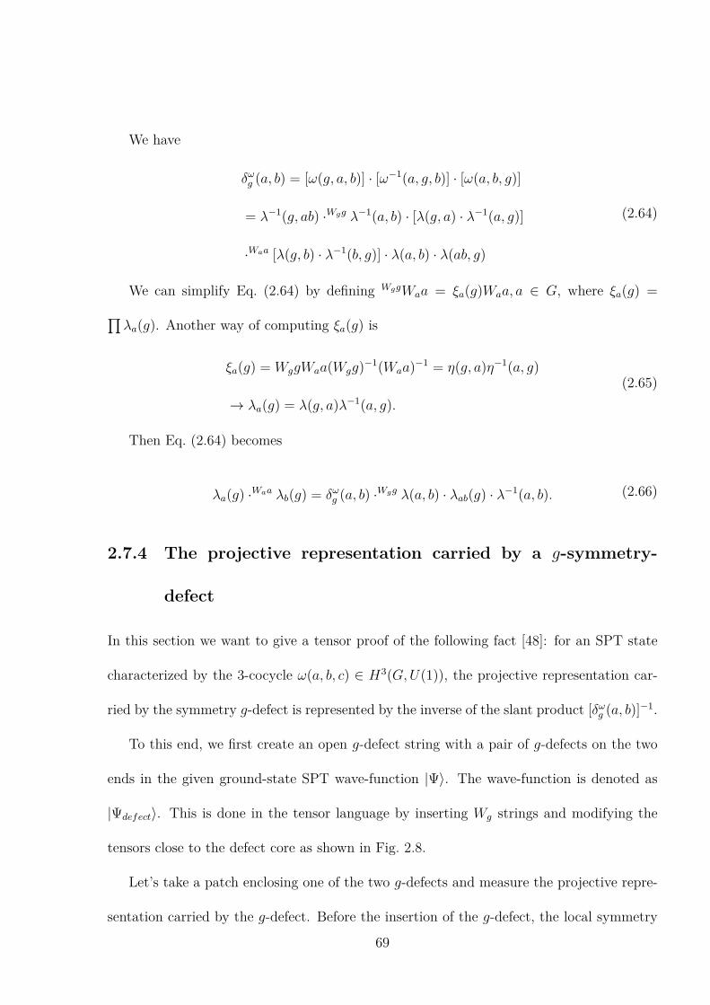
We have
δωg (a, b) = [ω(g, a, b)] · [ω−1(a, g, b)] · [ω(a, b, g)]
= λ−1(g, ab) ·Wgg λ−1(a, b) · [λ(g, a) · λ−1(a, g)]
·Waa [λ(g, b) · λ−1(b, g)] · λ(a, b) · λ(ab, g)
(2.64)
We can simplify Eq. (2.64) by defining WggWaa = ξa(g)Waa, a ∈ G, where ξa(g) =∏λa(g). Another way of computing ξa(g) is
ξa(g) = WggWaa(Wgg)−1(Waa)
−1 = η(g, a)η−1(a, g)
→ λa(g) = λ(g, a)λ−1(a, g).
(2.65)
Then Eq. (2.64) becomes
λa(g) ·Waa λb(g) = δωg (a, b) ·Wgg λ(a, b) · λab(g) · λ−1(a, b). (2.66)
2.7.4 The projective representation carried by a g-symmetry-
defect
In this section we want to give a tensor proof of the following fact [48]: for an SPT state
characterized by the 3-cocycle ω(a, b, c) ∈ H3(G,U(1)), the projective representation car-
ried by the symmetry g-defect is represented by the inverse of the slant product [δωg (a, b)]−1.
To this end, we first create an open g-defect string with a pair of g-defects on the two
ends in the given ground-state SPT wave-function |Ψ⟩. The wave-function is denoted as
|Ψdefect⟩. This is done in the tensor language by inserting Wg strings and modifying the
tensors close to the defect core as shown in Fig. 2.8.
Let’s take a patch enclosing one of the two g-defects and measure the projective repre-
sentation carried by the g-defect. Before the insertion of the g-defect, the local symmetry
69
action U(a) on the patch is defined as acting Wa on the virtual legs on the edge and D(a)
on the physical legs inside the patch, i.e.,
U(a) =∏
boundaryWa
∏bulk
D(a). (2.67)
The symmetry operation should leave |Ψ⟩ invariant up to a phase. Then the projective
representation inside the patch is measured by acting
D(a) ·D(b) · [D(a b)]−1 (2.68)
on the physical legs inside the patch. Alternatively, we can do this by monitoring the
inverse of the phase generated by acting η(a, b) ≡ Wa ·a Wb · (Wab)−1 on the boundary
virtual legs since, by our assumption, the action of U(a)U(b)U(ab)−1 leaves the patch fully
invariant.
In general , acting η(a, b) on the virtual legs of a tensor leaves the tensor invariant only
up to a phase. Therefore η itself is not a global IGG. Instead, we have
η(a, b) = Wx(a, b)η′(a, b), (2.69)
where Wx(a, b) is a pure-phase gauge transformation which yields the extra phase for each
site and η′(a, b) leaves every tensor invariant. Now η′(a, b) is decomposable and we denote
it as η′(a, b) =∏λp(a, b).
As for our present case, suppose we have the action of∏
boundaryη(a, b) on the ground
state wave-function ∏boundary
η(a, b) |Ψ⟩ = eiϕ |Ψ⟩ , (2.70)
from which we know that the projective representation inside the patch is just∏
bulk(D(a) ·
D(b) · [D(a b)]−1) = e−iϕ.
70

From the previous discussion we have
e−iϕ∏
boundaryη(a, b) =
∏boundary
η′(a, b). (2.71)
After the insertion of g-defect, the new local symmetry operation U g(a) should be
defined as acting Wa on the virtual legs on the edge and D(a) on the physical legs inside
the patch. Here we have used the Wa as shown in Fig. 2.9 where Wa on the bond crossing the
defect line is changed to be [λa(g)](d) ·Wa and remains Wa elsewhere. This newly-defined
Wa ensures that no boundary excitations are created. The physical symmetry operation in
the bulk should still be the same.
We will then use∏
boundary η(a, b) to measure the projective representation inside the
patch, where η(a, b) ≡ Wa ·a Wb · (Wab)−1. Far away from the defect core, the tensor
wave-function is basically the same as before. And∏
boundary η(a, b) will be the same as∏boundary η(a, b) except at the bond crossing the defect line, see Fig. 2.10. The η(a, b) at
the bond crossing the defect line should be Wa ·a Wb · (Wab)−1:
[λa(g)](d) ·Wa ·a [λb(g)](d) ·a Wb · ([λab(g)](d) ·Wab)−1
= [λa(g)](d) ·Waa [λb(g)](d) ·Wa ·a Wb · (Wab)−1[λ−1
ab (g)](d)
= [λa(g)](d) ·Waa [λb(g)](d) · η(a, b) · [λ−1ab (g)](d).
(2.72)
We can work with the decomposable η′(a, b) at the boundary if we keep track of the eiϕ
phase. After going through the calculation as shown in Fig. 2.10, we have
∏bdr
η(a, b) |Ψdefect⟩ = eiϕδωg (a, b) |Ψdefect⟩ . (2.73)
Comparing Eq. (2.70) with Eq. (2.73) and note that projective representation is defined
through the inverse of Eq. (2.70), we know that the g-defect carries [δωg (a, b)]−1 projective
representation.
71

2.7.5 Consequence of the magnetic translation symmetry in tensor-
network formulation
The magnetic translation symmetry and on-site projective representation constrain the
possible symmetric short-range entangled states in a system. Specifically, we have the
following fact: for a system with on-site projective representation of the on-site symmetry
group G characterized by α(a, b) and magnetic translation symmetry TxTyT−1x T−1
y = g, an
SPT ground state described by the 3-cocycle ω ∈ H3(G,U(1)) can be realized as its ground
state only when δωg (a, b) = α(a, b)−1.
Basic set-up We have TxTyT−1x T−1
y = g, which leads to
WTxTxWTyTy(WTxTx)−1(WTyTy)
−1 = Wgg. (2.74)
We define η(a, b) as
Wa ·a Wb = η(a, b)Wab. (2.75)
By acting η(a, b) on T, we will get an extra phase α(a, b)−1 per unit-cell, therefore it is
not a global IGG. However, we can define a pure-phase gauge transformation W (α(a, b))
which yields exactly the phase α(a, b)−1 for every site tensor, see Fig. for an illustration.
Then we can write η(a, b) as
η(a, b) = W (α(a, b))η′(a, b), (2.76)
where η′(a, b) =∏λ(a, b) is an IGG and is decomposable.
Similarly since we have D(g) D(a) = γa(g)D(a) D(g) on physical leg, where γa(g) =
α(g, a)/α(a, g) ∈ H1(G,U(1)). We write the action of Wgg on Waa as
WggWaa = W (γa(g))ξa(g) ·Waa, (2.77)
72

where ξg(a) =∏λg(a) is a decomposable IGG element and the definition of W (γa(g)) is
the same as W (α(a, b)).
And as for Tx, Ty, we have
WTxTxWaa = W (γa(Tx))ξa(Tx)Waa, etc.. (2.78)
We act Eq. (2.74) on Waa and obtain an IGG equation
Wggξ−1a (Ty) ·WggWTyTy ξ−1
a (Tx) ·WTxTx ξa(Ty) · ξa(Tx) = ξa(g), (2.79)
which, when lift to plaquette IGG, should give us (we have absorbed the phase ambiguity
into the definition of λa(g))
Wggλ−1a (Ty) ·WggWTyTy λ−1
a (Tx) ·WTxTx λa(Ty) · λa(Tx) = λa(g). (2.80)
Acting Wgg We first act Wgg on Eq. (2.75), then we have
Wgg[WaaWbb] =Wgg [η(a, b)Wabab]
⇒ W (γa(g)) ·a W (γb(g))ξa(g) ·Waa ξb(g) ·WaaWbb
=Wgg η(a, b) ·W (γab(g))ξab(g)Wabab,
(2.81)
which then leads to
ξa(g) ·Waa ξb(g) =Wgg η′(a, b) · ξab(g) · η′−1(a, b), (2.82)
where extra phase factors W (α(a, b)), W (γa(g)) all cancel.
When lifting Eq. (2.82) to plaquette, we have (from Eq. (2.66))
λa(g) ·Waa λb(g) = δωg (a, b) ·Wgg λ(a, b) · λab(g) · λ(a, b)−1. (2.83)
Acting translation We have another way of deriving Eq. (2.83). We first act WTxTx
on the two sides of Eq. (2.75) and obtain an IGG equation,
ξa(Tx) ·Waa ξb(Tx) =WTxTx η(a, b) · ξab(Tx)η(a, b)−1, (2.84)
73

where the extra W (γa(Tx)),W (γb(Tx)),W (γab(Tx)) cancel since we have γa(Tx) ·a γb(Tx) =
γab(Tx).
When lift Eq. (2.84) to plaquette IGG, we have
λa(Tx) ·Waa λb(Tx) = [α(a, b)]−y ·WTxTx λ(a, b)λab(Tx)λ−1(a, b), (2.85)
where∏[α(a, b)]−y =WTxTx W (α(a, b)) ·W (α(a, b))−1 and the plaquette IGG [α(a, b)]−y are
just loops of phases as shown in Fig. 2.12.
Similarly we have
λa(Ty) ·Waa λb(Ty) =WTyTy λ(a, b)λab(Ty)λ
−1(a, b), (2.86)
where there is no extra factor coming from WTyTyW (α(a, b)) ·W (α(a, b))−1 since it is Ty
invariant.
With Eq. (2.85) and Eq. (2.86) we can explicitly calculate the action of
WTxTxWTyTy(WTxTx)−1(WTyTy)
−1
on Eq. (2.75) in terms of plaquette IGG. The action of WTxTxWTyTy(WTxTx)−1(WTyTy)
−1
74

on LHS of Eq. (2.75) is
Wgg[λa(Ty) ·Waa λb(Ty)]−1 ·WggWTyTy [λa(Tx)
Waaλb(Tx)]−1
·WTxTx [λa(Ty)Waaλb(Ty)] · [λa(Tx)Waaλb(Tx)]
=WggWaa λ−1b (Ty) ·Wgg [λ−1
a (Ty) ·WTyTyWaa λ−1b (Tx)
WTyTyλ−1a (Tx)]
·WTxTx λa(Ty) ·WTxTxWaa λb(Ty) · λa(Tx)Waaλb(Tx)
= λa(g)WaaWggλ−1
b (Ty) · λ−1a (g) ·Wgg [WaaWTyTyλ−1
b (Tx)λ−1a (Ty)
WTyTyλ−1a (Tx)]
·WTxTx λa(Ty) · λa(Tx)
·WaaWTxTx λb(Ty) ·Waa λb(Tx)
= λa(g) ·WaaWgg λ−1b (Ty) ·WaaWggWTyTy λ−1
b (Tx) · [λ−1a (g)Wggλ−1
a (Ty)WggWTyTyλ−1
a (Tx)
·WTxTx λa(Ty)λa(Tx)]
·WaaWTxTx λb(Ty)Waaλb(Tx)
= λa(g) ·Waa [Wggλ−1b (Ty) ·WggWTyTy λ−1
b (Tx) ·WTxTx λb(Ty)λb(Tx)]
= λa(g) ·Waa λb(g),
(2.87)
where we have used Eq. (2.77) and Eq. (2.78) in the first three equalities and we have used
Eq. (2.80) in the last two equalities.
75

The action of WTxTxWTyTy(WTxTx)−1(WTyTy)
−1 on RHS of Eq. (2.75) is
Wgg[WTyTyλ(a, b)λab(Ty)λ−1(a, b)]−1 ·WggWTyTy [α(a, b)−y
·WTxTx λ(a, b)λab(Tx)λ−1(a, b)]−1
·WTxTx [WTyTyλ(a, b)λab(Ty)λ−1(a, b)] · α(a, b)−y ·WTxTx λ(a, b)λab(Tx)λ
−1(a, b)
=WTyTy [α(a, b)−y]−1 · α(a, b)−y ·Wgg λ(a, b)Wggλ−1ab (Ty)
·WggWTyTy λ−1ab (Tx) ·
WTxTx λab(Ty) · λab(Tx) · λ−1(a, b)
= α(a, b)−1 ·Wgg λ(a, b) · λab(g) · λ−1(a, b),
(2.88)
where we have used Eq. (2.80) and α−1(a, b) is just a plaquette IGG with loop of phases
α−1(a, b).
Combining Eq. (2.87) with Eq. (2.88), we have
λa(g) ·Waa λb(g) = α−1(a, b)Wggλ(a, b) · λab(g) · λ−1(a, b). (2.89)
Comparing Eq. (2.89) with Eq. (2.83), we have
α−1(a, b) = δωg (a, b). (2.90)
It is easy to see that the global phase ambiguities in Eq. (2.80),(2.85),(2.86) will at most
modify the LHS of Eq. (2.90) up to a 2-cobounday, therefore it should be understood as
the 2-cycle equivalence δωg ≃ α−1 ∈ H2(G,U(1)).
2.7.6 Generic constructions of symmetry-enforced SPT tensor-
network wavefunctions
In this section we want to construct an SPT state with on-site symmetry group G, magnetic
translation symmetry satisfying TxTyT−1x T−1
y = g where the SPT is characterized by the
76

3-cocycle ω ∈ H3(G,U(1)) and the on-site symmetry group is represented projectively with
the 2-cocycle α(a, b) equal to the inverse of the slant product of ω with respect to g,i.e.,
α(a, b) ≃ [δωg (a, b)]−1 ∈ H2(G,U(1)). (2.91)
To achieve this goal, we will use the tensor network formalism. Let’s start from a
SPT tensor wavefunction with the symmetry group Z2 × G described by a 3-cocycle ω ∈
H3(G,U(1)), where Z2 represents the usual translation T orig.x , T orig.
y . Then we know that
every tensor is invariant under the action D(a) on physical leg together with∏Wa on all
the virtual legs, from which we have a set of tensor equations. Here we require D(a) to
be a direct sum of usual representation D1(a) and projective representation D2(a) with
2-cocycle [δωg (a, b)]−1. We choose the gauge transformation WT orig.
x,WT orig.
yto be identity
for simplicity. The global IGG η(a, b) comes from the following tensor equation:
Wa ·a Wb = η(a, b)Wab, (2.92)
where η(a, b) is decomposable, i.e., η(a, b) =∏λp(a, b). We require tensors to be fully
invariant under η(a, b) without even generating phases. This condition ensures D(a) on the
physical legs to be projected onto D1(a) sector.
We define WggWaa = ξa(g)Waa, where ξa(g) =∏λa(g) is a decomposable global IGG.
More generally we define (Wgg)xWa = ξa(g, x)Wa, where ξa(g, x) =∏λa(g, x). Then we
have the following relation:
λa(g, x+ 1) =Wgg λa(g, x) · λa(g). (2.93)
Then we change our tensor wave-function in the following way:
1. We revise the original tensor such that it is invariant under the symmetry operation
and the new plaquette IGG defined in Fig. 2.13. Note that this step is necessary for
77
us to obtain a symmetric and non-vanishing tensor wave-function after the insertion
of Wg.
2. We insert [Wg(u)]x on the upper leg of every tensor as shown in Fig. 2.14. Physically
it means inserting one g-defect per unit-cell.
3. We define the new on-site symmetry operation Wa and translation symmetry WTx
as shown in Fig. 2.14. We will show that the new tensor is invariant under such
symmetry transformations.
From the last section we have shown that every g-defect carries a projective represen-
tation represented by δωg (a, b)−1, therefore one would expect after insertion of g-defects, we
now have one δωg (a, b)−1 projective representation per unit-cell. Let’s show it more clearly
through explicit calculations.
First, let’s show that the revised tensor wave-function satisfies all the required symme-
tries. It’s apparent that the new tensor has magnetic translation symmetry WTxTx,WTyTy
defined in Fig. 2.14, i.e.
WTxTxWTyTy(WTxTx)−1(WTyTy)
−1 = Wgg. (2.94)
It can be proven that the new tensor is invariant under the new symmetry transfor-
mation Waa as shown in Fig. 2.15. The invariance of the new tensor T (x,y) under the new
plaquette IGG is also apparent as shown in Fig. 2.14. Then we know that Eq. (2.60) still
holds for this state, which means the new state obtained is still an SPT state described by
the same 3-cocycle ω.
Finally we want to show that the new tensor now carries a projective representation
[δωg (a, b)]−1 per unit-cell. It can be proven that by acting Wa ·a Wb · W−1
ab on all the virtual
78
legs of a tensor we will get a phase δωg (a, b) for every tensor as shown in Fig. 2.16.
In doing so we need the following identity
λa(g, x)Waaλb(g, x)λ(a, b)λab(g, x)
−1 ·(Wgg)x [λ(a, b)−1] = [δωg (a, b)]x. (2.95)
Let’s denote the LHS of Eq. (2.95) as f(x). From Eq. (2.66) we have f(1) = δωg (a, b),
then we need to find out the relation between f(x) and f(x + 1). Using λ(g, x) =Wgg
λ(g, x− 1) · λ(g), we can rewrite Eq. (2.95) as
[Wggλa(g, x− 1)λa(g)]Waa[Wggλb(g, x− 1) · λb(g)]λ(a, b)[Wggλab(g, x− 1) · λab(g)]−1 ·(Wgg)x [λ(a, b)−1]
= [Wggλa(g, x− 1)λa(g)]WaaWggλb(g, x− 1) ·Waa λb(g)λ(a, b)λab(g)
−1
· [Wggλab(g, x− 1)]−1 ·(Wgg)x [λ(a, b)−1]
=Wgg λa(g, x− 1)[λa(g)ξ−1a (g)]WggWaaλb(g, x− 1)ξa(g)
Waaλb(g)λ(a, b)λab(g)−1
·Wgg [λab(g, x− 1)]−1 ·(Wgg)x [λ(a, b)−1]
= δωg (a, b)Wggλa(g, x− 1)[λa(g)ξ
−1a (g)]WggWaaλb(g, x− 1)[ξa(g)λa(g)
−1]Wggλ(a, b)
·Wgg [λab(g, x− 1)]−1 ·(Wgg)x [λ(a, b)−1]
= δωg (a, b)Wgg[λa(g, x− 1)Waaλb(g, x− 1)λ(a, b) · λab(g, x− 1)−1 ·(Wgg)x−1
λ(a, b)−1].
(2.96)
The above derivation tells us that f(x) = δωg (a, b)Wggf(x − 1), therefore by induction
we have f(x) = [δωg (a, b)]x.
With the help of Eq. (2.95), we can readily calculate the new IGG η(a, b) ≡ Wa ·a Wb ·
W−1ab . The η(a, b) on the up and down virtual legs are just η(a, b) defined before. The
79

η(a, b) on the left leg is computed as follows:
[λa(g,−x)](d) ·Wa ·a [λb(g,−x)](d) ·a Wb · ([λab(g,−x)](d) ·Wab)−1
= [λa(g,−x)](d) ·Waa [λb(g,−x)](d) ·Wa ·a Wb · (Wab)−1[λab(g,−x)](d)−1
= [λa(g,−x)](d) ·Waa [λb(g,−x)](d) · η(a, b) · [λab(g,−x)](d)−1
= [δωg (a, b)]−x[λ(a, b)](u)−1 ·(Wgg)−x
[λ(a, b)](d).
(2.97)
Similarly, we have on the right leg
[δωg (a, b)]x+1 ·(Wgg)−x−1
[λ(a, b)](d)−1 · [λ(a, b)](u). (2.98)
Therefore, as shown in Fig. 2.16, we know that η(a, b) is just δωg (a, b) times the product
of plaquette IGG shown in Fig. 2.14 which leaves the tensor invariant up to a phase δωg (a, b).
Then on the physical leg we are forced to have D(a)D(b) = [δωg (a, b)]−1D(ab), i.e., D(a) is
projected onto D2(a) sector. So the desired on-site projective representation is achieved.
80

Figure 2.8: An example of g-defect line. The g-defect line is obtained by inserting Wg on
only one side of the virtual legs crossed by the red dashed line. The tensors close to the
defect core should be revised in order to make the tensor wave-function symmetric and non-
vanishing. Following the usual convention, we say that the defect line always points from
g−1-defect to g-defect, and we always insert Wg to the left when one goes forward along
the line. Therefore in the figure we can identify the right end as the g-defect (remember
Wg(d) = Wg(u)−1). The grey area encloses a g-defect and we can to measure its projective
representation through the action of η′(a, b) on the boundary virtual legs, see the discussion
in the main text.
81

Figure 2.9: Invariance of the wave-function under U g(a). In the figure we can see that
Wa = [λa(g)](d) ·Wa where the defect line crosses the boundary and Wa = Wa elsewhere.
Such a definition ensures that no boundary excitations are created by acting U g(a) (for
the moment we do not care about what happens at the defect core). In deriving the
second figure, we have used the invariance of the tensor under Waa, the identity WaW−1g =
W−1g ξa(g)Wa and invariance of the tensor under plaquette IGG λa(g).
82

Figure 2.10: Measurement of projective representation carried by g-defect. From Eq. (2.72),
we know that η(a, b) = λa(g) ·Waa λb(g) · η(a, b) · λ−1ab where the boundary is crossed by the
defect line and η(a, b) = η(a, b) elsewhere. In the first equality we have used Eq. (2.71).
In the second equality we have used the decomposition of η′(a, b) and Eq. (2.66). In the
third equality we have used the tensor invariance under plaquette IGG. In the last equality
we have used the identity λ(r)−1 ·W−1g = W−1
g ·Wg λ(r)−1 and the tensor invariance under
plaquette IGG.
83

Figure 2.11: The definition of phase-gauge transformation W (α(a, b)).
Figure 2.12: The decomposition rule of WTxTxW (α(a, b)) ·W (α(a, b))−1 (LHS) as a product
of plaquette IGG λ(α(a, b)) (RHS).
84

Figure 2.13: The original tensor before insertion of g-defect is required to be invariant
under the revised symmetry operation and the revised plaquette IGG.
85

Figure 2.14: (a) The definition of the new tensor T (x,y) after the insertion of [Wg(u)]x to
the upper leg of every original tensor T (x,y). (b) The new translation operation WTxTx.
It can be readily checked that T (x,y) is invariant under such translation. Note that we
have Tx = gyT orig.x , Ty = T orig.
y and WTy = 1. (c) The new on-site symmetry operation
Waa. It is shown in Fig. 2.15 that T (x,y) is invariant under such symmetry operation. (d)
The new plaquette IGG for the new tensor T (x,y). As before, λ’s from different plaquettes
commute with each other, and the action of any two λ’s in the same plaquette leave the
tensor invariant. The tensor T (x,y) invariance under plaquette IGGs follows trivially from
Fig. 2.13.
86

Figure 2.15: The revised tensor T (x, y) is invariant under the newly-defined symmetry op-
eration. The first equality comes from the commutation relation WaWxg = W x
g ξa(g,−x)Wa.
In the second equality we have used the invariance of tensor under Wa as shown in Fig. 2.13
and the decomposition of ξa(g,−x). In the third equality we have used the identity
λa(g,−x)(l) =Wgg [λa(g,−x − 1)](l) · λa(g)(l). And we have also used the invariance of
tensor under plaquette IGG as in Fig. 2.14 in the third and fourth equalities.
87

Figure 2.16: Every site-tensor carries a projective representation characterized by
[δωg (a, b)]−1. We show this by acting WaaWbb(Wabab)
−1 on both the physical legs and
the virtual legs of tensor T (x,y), which should leave the tensor invariant without gen-
erating any phase. But from the calculation we find that the action on vitrual legs
will contribute a factor δωg (a, b), therefore the representation on the physical legs are
D(a) ·D(b) = [δωg (a, b)]−1D(ab), i.e., they are projected onto the D2(a) sector with projec-
tive representation. In the calculation above, we have used Eq. (2.95) in the first equality.
And we have used the invariance of the tensor under the plaquette IGG defined in Fig. 2.14
in the second equality.
88

Bibliography
[1] E. Lieb, T. Schultz, and D. Mattis, Annals of Physics 16, 407 (1961).
[2] M. Oshikawa, Phys. Rev. Lett. 84, 1535 (2000).
[3] A. Paramekanti and A. Vishwanath, Phys. Rev. B 70, 245118 (2004).
[4] M. B. Hastings, Physical Review B 69, 104431 (2004).
[5] M. B. Hastings, EPL (Europhysics Letters) 70, 824 (2005).
[6] M. Zaletel, A. Vishwanath, Physical Review Letters, 114(7), 077201 (2015).
[7] M. Cheng, M. Zaletel, M. Barkeshli, A. Vishwanath, and P. Bonderson, arXiv preprint
arXiv:1511.02263 (2015).
[8] X.-L. Qi and S.-C. Zhang, Rev. Mod. Phys. 83, 1057 (2011).
[9] M. Z. Hasan and C. L. Kane, Rev. Mod. Phys. 82, 3045 (2010).
[10] I. Affleck et al. Physical Review B 87, 155114 (1987).
[11] X. Chen, Z.-C. Gu, Z.-X. Liu, and X.-G. Wen, Science 338, 1604 (2012),
[12] X. Chen, Z.-C. Gu, Z.-X. Liu, and X.-G. Wen, Phys. Rev. B 87, 155114 (2013).
89

[13] I. Dana, Y. Avron, and J. Zak, Journal of Physics C: Solid State Physics 18, L679
(1985).
[14] Y.-M. Lu, Y. Ran, and M. Oshikawa, Annals of Physics 413, 168060 (2020).
[15] J. Wu, T.-L. Ho, and Y.-M. Lu, arXiv preprint arXiv:1703.04776 (2017).
[16] D.-H. Lee and M. P. Fisher, Physical Review Letters 63, 903 (1989).
[17] Y.-M. Lu and A. Vishwanath, Phys. Rev. B 93, 155121 (2016).
[18] T. Senthil and M. Levin, Phys. Rev. Lett. 110, 046801 (2013).
[19] L. Balents, M. P. Fisher, and C. Nayak, Physical Review B 60, 1654 (1999).
[20] X.-G. Wen, Quantum
eld theory of many-body systems: from the origin of sound to an origin of light and
electrons (Oxford University Press on Demand, 2004).
[21] S. Jiang and Y. Ran, Physical Review B 95, 125107 (2017).
[22] K. Duivenvoorden, M. Iqbal, J. Haegeman, F. Verstraete, and N. Schuch, arXiv
preprint arXiv:1702.08469 (2017).
[23] L. Balents, M. P. A. Fisher, and S. M. Girvin, Phys. Rev. B 65, 224412 (2002).
[24] D. Sheng and L. Balents, Physical Review Letters 94, 146805 (2005).
[25] S. Isakov, Y. B. Kim, and A. Paramekanti, Physical review letters 97, 207204 (2006).
[26] E. Fradkin, Field theories of condensed matter physics (Cambridge University Press,
2013).
90

[27] D. S. Rokhsar and S. A. Kivelson, Physical review letters 61, 2376 (1988).
[28] SPT phases protected by G = SO(3)×ZIsing2 form a group H3(SO(3)×ZIsing
2 , U(1)).
The Kunneth formula gives: H3(SO(3) × ZIsing2 , U(1)) = H3(SO(3), U(1)) ×
H3(Z2, U(1)) × H2(SO(3), Z2) = Z × Z2 × Z2. Following the Remark, it is straight-
forward to show that only the Z2 index in H2(SO(3), Z2) is enforced to be non-
trivial. (Namely ω0 in Theorem-(2) can be chosen to be the nontrivial element in
H2(SO(3), Z2),and the kernal Ag = H3(SO(3), U(1))×H2(SO(3), Z2) = Z × Z2.)
[29] Following the Kunneth formula: H3(ZT2 × ZIsing
2 , U(1)) = H3(ZT2 , U(1)) ×
H3(Z2, U(1))×H2(ZT2 , Z2) = Z1×Z2×Z2. In this example, the Z2 index in H2(ZT
2 , Z2)
is enforced to be nontrivial, and the Z2 index in H3(Z2, U(1)) is enforced to be trivial.
This is because here ω0 in Theorem-2 is the nontrivial element in H2(ZT2 , Z2), and the
kernel subgroup Ag = Z1.
[30] X. Chen, Y.-M. Lu, and A. Vishwanath, Nature commu- nications 5 (2014).
[31] Now in this example, ω0 in Theorem-2 is the nontrivial element in H3(Z2, U(1)), and
the kernel subgroup Ag = Z1.
[32] R. Moessner and S. L. Sondhi, Phys. Rev. Lett. 86, 1881 (2001).
[33] Y. Qi, Z.-C. Gu, and H. Yao, Physical Review B 92, 155105 (2015).
[34] R. Moessner and S. Sondhi, Physical Review B 63, 224401 (2001).
[35] R. Moessner, S. L. Sondhi, and E. Fradkin, Physical Re- view B 65, 024504 (2001).
[36] R. Moessner, S. Sondhi, and P. Chandra, Physical review letters 84, 4457 (2000).
91

[37] J. B. Kogut, Reviews of Modern Physics 51, 659 (1979).
[38] A. Y. Kitaev, Annals of Physics 303, 2 (2003).
[39] M. Levin and Z.-C. Gu, Phys. Rev. B 86, 115109 (2012).
[40] D. Perez-Garcia et al. New J. Phys. 12, 025010 (2010).
[41] H. Zhao, Z. Xie, Q. Chen, Z. Wei, J. Cai, and T. Xiang, Physical Review B 81, 174411
(2010).
[42] S. Singh, R. N. C. Pfeifer, and G. Vidal, Phys. Rev. A 82, 050301 (2010).
[43] S. Singh, R. N. Pfeifer, and G. Vidal, Physical Review B 83, 115125 (2011).
[44] S. Singh and G. Vidal, Physical Review B 86, 195114 (2012).
[45] B. Bauer et al. Physical Review B 83, 125106 (2011).
[46] A. Weichselbaum, Annals of Physics 327, 2972 (2012).
[47] S. Jiang and Y. Ran, Phys. Rev. B 92, 104414 (2015).
[48] M. P. Zaletel, Physical Review B 90, 235113 (2014).
[49] F. Pollmann, A. M. Turner, E. Berg, and M. Oshikawa, Phys. Rev. B 81, 064439
(2010).
[50] X. Chen, Z.-C. Gu, and X.-G. Wen, Phys. Rev. B 83, 035107 (2011).
92

Chapter 3
Divergent bulk photovoltaic effect in
Weyl semimetals
3.1 Introduction
Weyl semimetals are a class of materials that can be regarded as three-dimensional analogs
of grapheneupon breaking time-reversal or inversion symmetry. Electrons in a Weyl semimetal
behave as Weylfermions, which have many exotic properties, such as chiral anomaly and
magnetic monopoles in thecrystal momentum space. The surface state of a Weyl semimetal
displays pairs of entangled Fermi arcs at two opposite surfaces. To linear order, the
electrons near a Weyl node can be described by the effective two-by-two Hamiltonian:
HWeyl = (∑
a kaαa − µ)σ0 +
∑a,b k
aβabσb, where µ is the chemical potential, k is the mo-
mentum relative to the Weyl node, a/b = x, y, z, σb are the Pauli matrices and σ0 is the
identity matrix. After choosing the frame of the principal axes and a proper basis, the
93

off-diagonal elements in β can be eliminated:
HWeyl = (~k · vt − µ) σ0 + ~∑a
(kavaσa). (3.1)
Here apart from the generally anisotropic velocity v, another velocity vt describes the tilting
of the bands and breaks the degeneracy between the bands at k and −k, with the chemical
potential (µ) usually nonzero.
It is known that either inversion symmetry or time-reversal symmetry needs to be broken
in order to realize the Weyl nodes, and the experimentally confirmed Weyl semimetals
have been overwhelmingly non-centrosymmetric and time-reversal symmetric, including the
(Nb,Ta)(As,P) and W1−xMoxTe2 series [2–8]. When the tilting velocity is large enough,
which is realized in materials like W1−xMoxTe2, the system can becomes a Type-II WSM [7],
since along some directions the two energy bands share the same sign of the velocity. Such
a system must have finite size Fermi surfaces (Fig.3.1(d))1. The type of a Weyl node is
determined by a dimensionless number W :
W ≡√
(vxt /vx)2 + (vyt /v
y)2 + (vzt /vz)2, (3.2)
and a Type-I(Type-II) Weyl node is realized if W < 1 (W > 1).
As we show later, the bulk photovoltaic effect [10] with its direct connection to Berry
curvature, [?, 11] offers a method to distinguish these two types. It has also attracted
significant interest due to its potential applications in renewable energy generation [12] and
fast photo-detectors [13,14]. The intrinsic contributions to the BPVE can be expressed as
1Consequently it may be more accurate to call it a Type-II Weyl metal instead of a semimetal. However
to be consistent with existing literature we follow the existing naming convention.
94

the second order nonlinear photocurrent response:
ja = σabc2 (ω)Eb(ω)Ec(−ω), (3.3)
where, a/b/c = x, y, z, −→j is the DC electric current density, E(t) = Re[E(ω)e−iωt +
E(−ω)eiωt] is the electric field of the light. In order to have a nonzero σ2, inversion sym-
metry needs to be broken, which happens to be also a condition to realize WSM. Generally
speaking, σabc2 has both intraband and interband contributions. However, for time-reversal
symmetric materials with linear polarized light, it turns out that this photocurrent response
only has interband contributions, which has been coined the shift-current(σabc2 = σabc
shift) as
it results from a change in the center of mass of the electrons upon optical excitation.
Perturbation theory within the single-particle framework [11, 15, 16] gives:
σabcshift(ω) =
2πe3
~2
∫d3k
(2π)3
∑n,m
Iabcmn[fnm · δ(ωmn − ω)], (3.4)
where n,m label energy bands, ~ωmn(k) ≡ Em(k)−En(k) is the energy difference between
the two bands. fnm(k) = fn(k) − fm(k) is the difference of the Fermi-Dirac function
between the two bands. The gauge invariant quantity Iabcmn(k) ≡ 12· Im[rbmnr
cnm;a+r
cmnr
bnm;a],
where ramn(k) ≡ i⟨um(k)|∂ka |un(k)⟩ is nothing but the non-Abelian Berry’s connection
(with ramn;b(k) its generalized derivative: ramn;b ≡ ∂ramn
∂kb− i[Ab
m(k) − Abn(k)]r
amn(k), and
Abn(k) ≡ i⟨un(k)|∂kb|un(k)⟩ the usual intraband Berry’s connection).
It has been pointed out that the shift current response is related to the topology of the
band structure [?]. Indeed the quantities responsible for σshift directly involves the Abelian
and non-Abelian Berry’s phases. Because Weyl nodes are monopoles of the Abelian Berry’s
connection, these quantities are expected to be diverging and singular near Weyl nodes,
which motivates us to carefully study the resulting nonlinear optical effects.
95

Eq.(3.4) has a familiar form of the Fermi’s golden rule. Indeed, considering the case of
linearly polarized light along the b-direction, one has:
Iabbmn = |rbnm|2Ranm,b, (no summation on indices) (3.5)
where the gauge invariant real space displacement Rnm,b(k) is the so-called “shift-vector”,
defined as:
Ranm,b(k) ≡ −∂Arg[rbnm]
∂ka+ Aa
n(k)− Aam(k), (3.6)
If one interprets Eq.(3.4,3.5) as the Fermi’s golden rule, |rbnm|2 is just the matrix-element
factor for the optical absorption. Thus, eRnm,b(k) should be viewed as the dipole moment
induced the photo-excited particle-hole pair, giving rise to a rate of change in polarization,
i.e., DC photocurrent.
Motivated by photogalvanic applications [12–14], previously the shift-current response
has been mainly discussed in the context of insulators [11, 16], where the low temperature
σshift vanishes when ~ω is below the band gap. It is convenient to introduce the optical
joint density of states including the factor fnm responsible for the Pauli-blocking effect:
JDOS(ω) ≡∫
d3k
(2π)3
∑m,n
[fnm · δ(ωmn − ω)] (3.7)
For most materials, Iabcmn(k) is a smooth function of momentum, and according to Eq.(3.4)
the response σshift is essentially proportional to JDOS. It has been proposed that engi-
neering JDOS in semiconductors may be a route to optimize the BPVE [17]. Although
the JDOS ∝ ω2 is small due to the linear dispersion in WSM, recent second harmonic [18]
and photocurrent experiments [?,19] show that these materials host large nonlinear optical
effects at least in the infrared regimes. In this chapter we show that the WSM actually fea-
96
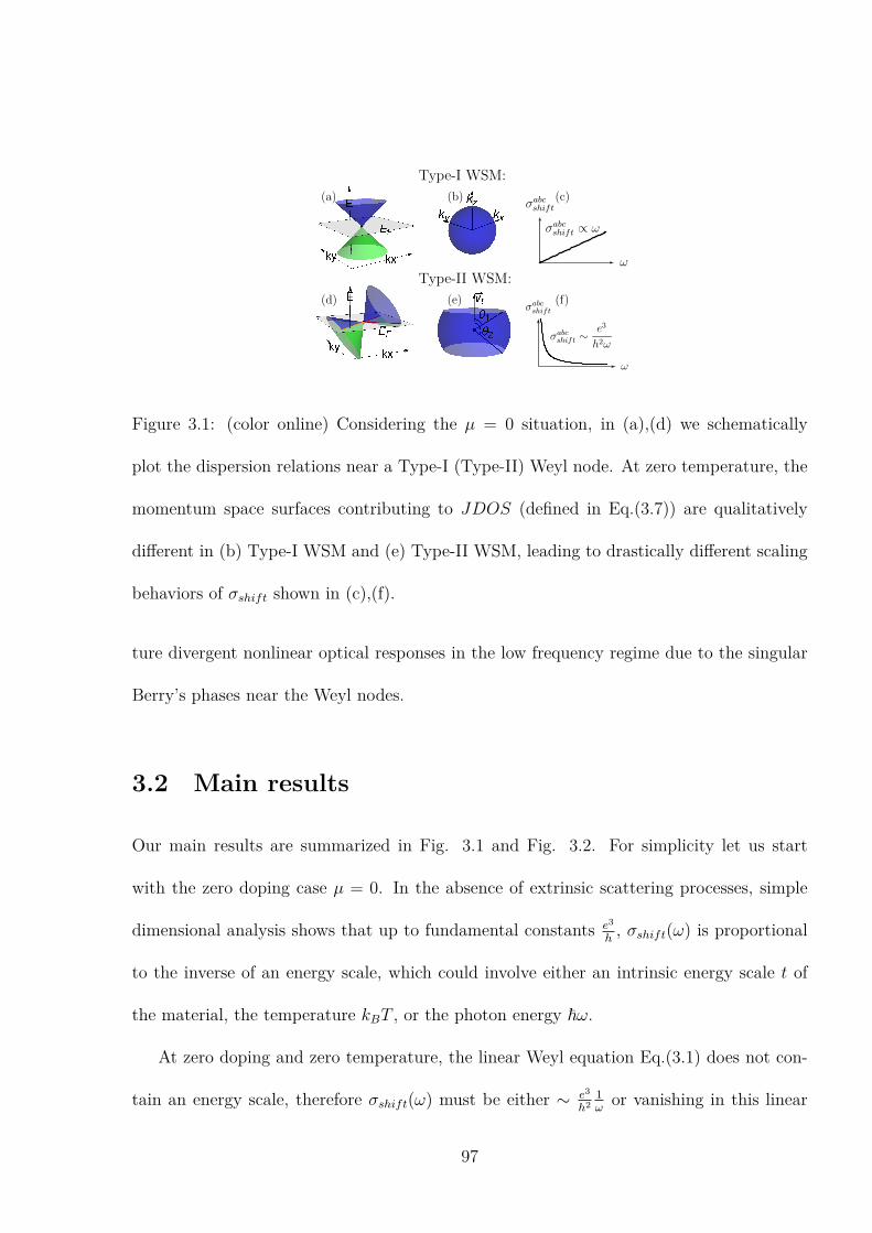
(a) (b)
Type-I WSM:
(c)
(d) (e)
Type-II WSM:
(f)
Figure 3.1: (color online) Considering the µ = 0 situation, in (a),(d) we schematically
plot the dispersion relations near a Type-I (Type-II) Weyl node. At zero temperature, the
momentum space surfaces contributing to JDOS (defined in Eq.(3.7)) are qualitatively
different in (b) Type-I WSM and (e) Type-II WSM, leading to drastically different scaling
behaviors of σshift shown in (c),(f).
ture divergent nonlinear optical responses in the low frequency regime due to the singular
Berry’s phases near the Weyl nodes.
3.2 Main results
Our main results are summarized in Fig. 3.1 and Fig. 3.2. For simplicity let us start
with the zero doping case µ = 0. In the absence of extrinsic scattering processes, simple
dimensional analysis shows that up to fundamental constants e3
h, σshift(ω) is proportional
to the inverse of an energy scale, which could involve either an intrinsic energy scale t of
the material, the temperature kBT , or the photon energy ~ω.
At zero doping and zero temperature, the linear Weyl equation Eq.(3.1) does not con-
tain an energy scale, therefore σshift(ω) must be either ∼ e3
h21ω
or vanishing in this linear
97
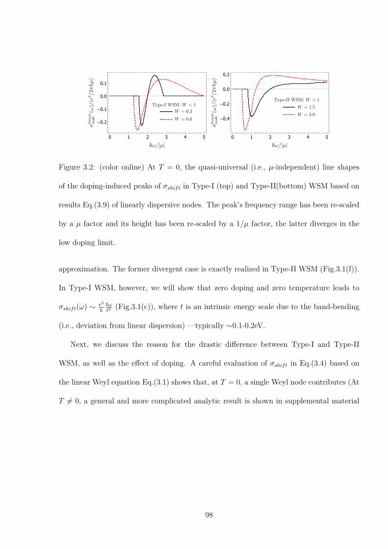
0 1 2 3 4 5
-0.2
-0.1
0.0
0.1
0 1 2 3 4 5
-0.4
-0.2
0.0
0.2
Figure 3.2: (color online) At T = 0, the quasi-universal (i.e., µ-independent) line shapes
of the doping-induced peaks of σshift in Type-I (top) and Type-II(bottom) WSM based on
results Eq.(3.9) of linearly dispersive nodes. The peak’s frequency range has been re-scaled
by a µ factor and its height has been re-scaled by a 1/µ factor, the latter diverges in the
low doping limit.
approximation. The former divergent case is exactly realized in Type-II WSM (Fig.3.1(f)).
In Type-I WSM, however, we will show that zero doping and zero temperature leads to
σshift(ω) ∼ e3
h~ωt2
(Fig.3.1(c)), where t is an intrinsic energy scale due to the band-bending
(i.e., deviation from linear dispersion) —typically ∼0.1-0.2eV.
Next, we discuss the reason for the drastic difference between Type-I and Type-II
WSM, as well as the effect of doping. A careful evaluation of σshift in Eq.(3.4) based on
the linear Weyl equation Eq.(3.1) shows that, at T = 0, a single Weyl node contributes (At
T = 0, a general and more complicated analytic result is shown in supplemental material
98

Eq.(3.35,3.36)):
σabcshift =
πχ
8W 2·∑d
[ϵdca
vbtvdt
(vd)2+ (b↔ c)
]· σlinear
node (ω) (3.8)
where:
σlinearnode ≡ (cos[θ1]sin[θ1]2 − cos[θ2]sin[θ2]2) ·
e3
h2ω, (3.9)
and: θ1 ≡ arccos[ 2µ~ω + 1
W
], θ2 ≡ arccos
[ 2µ~ω − 1
W
]. (3.10)
Up to an order unity constant σabcshift(ω) is determined by σlinear
node (ω). Here W is defined in
Eq.(3.2), ϵabc is the Levi-Civita antisymmetric tensor, and we have chosen the convention
ω > 0. χ ≡ sign[vxvyvz] = ±1 is the chirality of the Weyl node (i.e., monopole charge).
Note that we have chosen the frame x, y, z to be right-handed. We have also defined a
function arccos[s] ≡ 0 if s ⩾ 1, arccos[s] ≡ π if s ⩽ −1, and arccos[s] ≡ arccos[s] if
−1 < s < 1.
Interestingly, due to the chirality factor in this result, we know that this 1/ω divergent
term is absent in Dirac semimetals, because in those systems each Dirac node can be viewed
as two Weyl nodes with opposite chiralities sharing the same set of µ, vt and opposite v.
It can also be immediately seen from Eq. (3.8) that the 1/ω divergence is absent for σaaashift
due to the Levi-Civita antisymmetric tensor.
The physical meaning of the two angles θ1,θ2 is the following. For the moment it is
convenient to re-scale the momentum in x, y, z directions so that vx = vy = vz = v. The
energy conservation δ(ωmn − ω) constrains our consideration on a sphere in the re-scaled
momentum space, whose radius equals 2ωv
. The re-scaled vt can be used to define a special
axis to set up a spherical coordinate system. Generally speaking, Pauli blocking takes over
in certain solid angle regions. Namely the factor fnm further constrains the sphere into a
99

region between the polar angles θ1 and θ2 (See Fig.3.1(e) for an illustration).
In Type-I WSM (W < 1) at zero doping, the whole sphere contributes, consistent with
θ1 = 0 and θ2 = π (Fig.3.1(b)). But this is exactly a situation when the θ-dependent
factor in Eq.(3.9), and thus the 1/ω term in σshift, vanishes. (Note that, in this case, a
careful analysis including band-bending effects shows that even the constant order vanishes,
leaving the next order σshift ∝ ω in the low frequency limit. See supplemental information.)
But in Type-II WSM (W > 1) at zero doping, only the part of the sphere between θ1,2 =
arccos[± 1W] contributes (Fig.3.1(e)), leading to the 1/ω divergent response.
This results from the strongly angle dependent diverging Berry connection in WSM,
despite the integrand Iabcmn in Eq.(3.4) scaling as 1ω3 . The full angular average over the 4π
solid angle would annihilate the 1/ω term in σshift. However, Pauli-blocking could take
over in certain angular regions, removing the net cancellation and retaining the divergent
term.
In particular, at T = 0, in Type-I WSM (W < 1) with finite µ, this 1/ω term survives
only over a frequency range: 2|µ|1+W
⩽ ~ω ⩽ 2|µ|1−W
. (Thus in the extreme case when vt = 0 and
W = 0, this term vanishes.) In fact, it is straightforward to show that, σlinearnode would also
change sign exactly at ~ω = 2|µ|. Altogether this leads to a large peak in the σshift(ω) with
a width ∼ |µ|/~ and a height ∼ e3
h· 1|µ| , featuring a characteristic sign-changing line-shape
(Fig.3.2 top). Similarly a finite µ truncates the 1/ω divergence in Type-II WSM and leads
to a sign-changing large peak when ~ω ∼ µ (Fig.3.2 bottom).
As shown in Fig.3.2, the line-shapes of these peaks are quasi-universal: they only depend
on the dimensionless number W . Different values of doping µ only re-scale the peak’s
frequency range by a µ factor and its height by a 1/µ factor. This means that one may
100

use µ to control the frequency range of the peak to engineer tunable frequency-sensitive
photo-electric devices.
Temperature and impurities— At finite temperatures, the Fermi-Dirac distribution
would smear out and truncate the divergences when ~ω ≲ kBT (which is confirmed in
our tight-binding model calculations Fig.3.3). But at low temperatures kBT ≪ ~ω these
divergences are not significantly modified. (See supplemental material Eq.(3.35,3.36) for a
general analytic form of the σshift within linear-dispersion approximation.) However even
at zero temperature, impurities give rise to scattering, while finite temperature enables
other scattering mechanisms (e.g. electron-phonon). These scatterings, which can be phe-
nomenologically characterized by a scattering time τ , have been ignored so far. Namely,
even at low temperatures kBT ≪ ~ω our result Eq.(3.8) holds only in the long scattering
time ωτ ≫ 1 limit with the divergences truncated when ω ≲ 1τ. For instance, previous ex-
periments report that τ in the Type-I WSM TaAs is of the order of a pico-second [20, 21].
This suggests that our predicted striking response can be observed in the Terahertz or
higher frequency regimes.
A conceptually interesting situation occurs when a finite temperature is introduced in
the µ = 0 Type-I WSM, where divergence is absent at T = 0 due to angular cancellation
discussed before. However when T = 0, the thermally excited particle-hole pairs partially
play the role of doping, and there is no reason for a full angular cancellation. In this case,
simple dimensional analysis leads to striking results: we expect a temperature-induced peak
of the intrinsic σshift when ~ω ∼ kBT , whose height ∼ e3
hkBTdiverging in the low T limit.
(see supplemental material Eq.(3.35) and Fig.3.4) This is observed in our tight-binding
model calculations (see Fig.3.3(a)).
101

The size of the effects —It is interesting to estimate the size of effects in the divergent
regimes; e.g., when ~ω ∼ µ for Type-I WSM or ~ω ≳ µ in Type-II WSM, in the presence of
a temperature kBT ≪ ~ω. Previously shift-current responses have not be much studied in
the low frequency (e.g. Terahertz) regimes. Note that even in a generic multiband metal,
σshift is expected to vanish at zero temperature in the low frequency regimes. This is simply
because the energy conservation δ(ωmn − ω) and fnm in JDOS constrain both the valence
band and the conduction band at the Fermi level when ω → 0, which would not occur due
to band-repulsions.
Plugging in ω = 1THz, the estimated size of σshift ∼ e3
h21ω
in the divergent regimes is
∼ 0.01A/V 2, several orders of magnitudes larger than known reported values in visible or
infrared regimes [22–27]
Tight-binding model— To concretely illustrate the predicted responses we compute the
σshift tensor using a minimal time-reversal symmetric 4-band tight-binding model featuring
4 Weyl nodes: [18]
HTB = t[(2.5− cos kx − cos ky − cos kz)τx + sin kyτy
+ 0.5 cos kysxτy + sin kzsxτz + (ξ cos kx − µ0)]− µ, (3.11)
where sa(spin) and τa(orbital) are two sets of Pauli matrices. t is an overall energy scale
which can be 0.1 − 0.5eV, to be broadly consistent with the relevant energy scales in
existing Weyl materials. Symmetries in this model include: time-reversal isyK (K is
conjugation), x → −x mirror sx, and y → −y mirror syτx. The four Weyl nodes are
located at (kx = ±0.920, ky = ±0.464, kz = 0), with an energy µ0t and µ0 = 0.606ξ. A
positive parameter ξ controls the tilting velocity vt: for ξ < 1(ξ > 1), Type-I(Type-II)
WSM is realized. We choose ξ = 0.5 (ξ = 1.5), corresponding to W = 0.539(W = 1.616),
102
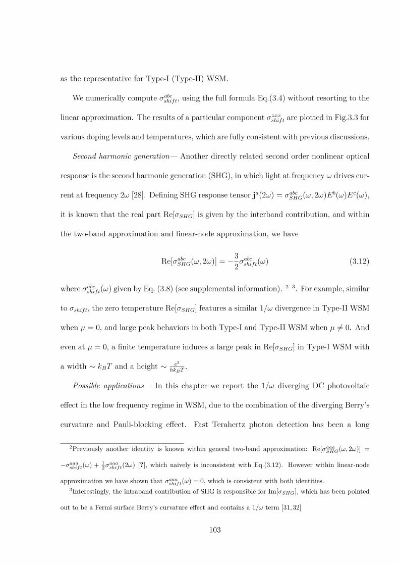
as the representative for Type-I (Type-II) WSM.
We numerically compute σabcshift, using the full formula Eq.(3.4) without resorting to the
linear approximation. The results of a particular component σzxxshift are plotted in Fig.3.3 for
various doping levels and temperatures, which are fully consistent with previous discussions.
Second harmonic generation— Another directly related second order nonlinear optical
response is the second harmonic generation (SHG), in which light at frequency ω drives cur-
rent at frequency 2ω [28]. Defining SHG response tensor ja(2ω) = σabcSHG(ω, 2ω)E
b(ω)Ec(ω),
it is known that the real part Re[σSHG] is given by the interband contribution, and within
the two-band approximation and linear-node approximation, we have
Re[σabcSHG(ω, 2ω)] = −3
2σabcshift(ω) (3.12)
where σabcshift(ω) given by Eq. (3.8) (see supplemental information). 2 3. For example, similar
to σshift, the zero temperature Re[σSHG] features a similar 1/ω divergence in Type-II WSM
when µ = 0, and large peak behaviors in both Type-I and Type-II WSM when µ = 0. And
even at µ = 0, a finite temperature induces a large peak in Re[σSHG] in Type-I WSM with
a width ∼ kBT and a height ∼ e3
hkBT.
Possible applications— In this chapter we report the 1/ω diverging DC photovoltaic
effect in the low frequency regime in WSM, due to the combination of the diverging Berry’s
curvature and Pauli-blocking effect. Fast Terahertz photon detection has been a long
2Previously another identity is known within general two-band approximation: Re[σaaaSHG(ω, 2ω)] =
−σaaashift(ω) +
12σ
aaashift(2ω) [?], which naively is inconsistent with Eq.(3.12). However within linear-node
approximation we have shown that σaaashift(ω) = 0, which is consistent with both identities.
3Interestingly, the intraband contribution of SHG is responsible for Im[σSHG], which has been pointed
out to be a Fermi surface Berry’s curvature effect and contains a 1/ω term [31,32]
103

standing challenge. The reported large photovoltaic effect may be useful for this purpose.
In addition, the doping-induced large peak regimes of σshift in WSM, whose frequency
ranges are controlled by µ, may be useful as a tunable frequency-sensitive probe for far-
infrared or Terahertz photons, i.e., a spectrum analyzer.
3.3 Appendices
3.3.1 Shift current in type-I Weyl semi-metal
In this section we shall prove that for a generic type-I Weyl semi-metal with Fermi level
at the Weyl nodes, the leading term in the shift current tensor will be proportional to ω
when ω → 0.
The low energy physics can be captured by the following generic 2-band Hamiltonian
with chemical potential µ set to zero
H = f0σ0 +∑
i=x,y,z
fiσi, (3.13)
where f0, fi are functions of k and fi = 0 when k = 0. The eigenvalues are Ec = f0 + ϵ,
Ev = f0 − ϵ with ϵ =√∑
i f2i . Since the tilting will not affect the shift current tensor, we
will set f0 to be zero.
The shift current tensor for the 2-band model is obtained by doing the following integral
[11, 17]
σabcshift(ω) =
2πe3
~2
∫d3k
(2π)3Iabccv [fcv · δ(ωcv − ω)], (3.14)
where Iabccv has the following explicitly gauge-invariant expression
Iabccv =∑i,j,m
[1
8ϵ3(fmfi,bfj,ac − fi,bfj,afm
ϵ,cϵ)ϵijm + (b↔ c)], (3.15)
104

where ϵijm is the Levi-Civita symbol.
Now let’s prove that terms proportional to 1/ω (denoted as σ(−1)(ω) below) and terms
independent of ω (denoted as σ(0)(ω) below) in σabc vanish in the low frequency limit ω → 0.
A simple order of estimate with k ∼ ω when ω → 0 tells us that only the k-linear terms
and k-quadratic terms in fi will contribute to σ(−1)(ω) and σ(0)(ω). Therefore it suffices to
consider a linear node plus some quadratic corrections. It is always possible to choose the
following form of fi by an affine transformation which does not affect the integral (~vF is
set to be 1 throughout this section)
fi = ki + αijlkjkl, (3.16)
where αijl is a rank-3 tensor symmetric respect to the interchange j ↔ l and repeated
indices are summed over.
In the spherical coordinate system, we have
kx = rsin[θ]cos[ϕ], ky = rsin[θ]sin[ϕ], kz = rcos[θ]. (3.17)
And the unit vector k = (sin[θ]cos[ϕ], sin[θ]sin[ϕ], cos[θ]) will be used below to simplify the
notation.
When ω is small, ki ∼ r ∼ ω and we can expand ϵ in powers of r
ϵ = r + r2f(θ, ϕ) +O(r3), (3.18)
where f(θ, ϕ) is a function of αijl, θ, ϕ. It is easy to obtain the explicit form of f(θ, ϕ), but
for our purpose we only need the fact that f(θ, ϕ) = −f(π − θ, π + ϕ) since it comes from
the angular dependence of terms involving 3 ki’s.
105

In the same spirit we can expand Iabc in powers of r
Iabc =1
8ϵ3[I
(0)abc + I
(1)abc +O(r2)], with
I(0) = −ϵbamkmkcϵ2
+ (b↔ c) = −ϵbamr2kmkcϵ2
+ (b↔ c),
I(1) = 2ϵbjmαjackm +habc(kx, ky, kz)
ϵ2+ (b↔ c) = 2rϵbjmαjackm + r3
habc(kx, ky, kz)
ϵ2+ (b↔ c)
(3.19)
where habc(kx, ky, kz) is a homogeneous polynomial of degree 3, whose explicit form, for our
purpose, is not important.
The integral then becomes
σabc(ω) = const ∗∫dΩ(
∫r2drIabc(r, θ, ϕ)δ(2ϵ(r, θ, ϕ)− ω)), (3.20)
where dΩ = sin[θ]dθdϕ.
When ω → 0, we know that for any fixed θ, ϕ there is only one solution r(θ, ϕ) to the
equation 2ϵ(r(θ, ϕ), θ, ϕ) = ω, from which we can solve r as a function of θ and ϕ. In fact,
we can expand r(θ, ϕ) in powers of ω with f(θ, ϕ) defined before
r(θ, ϕ) =ω
2− ω2
4f(θ, ϕ) +O(ω3). (3.21)
The integral can then be written as
σabc(ω) = const ∗∫dΩ
1
ω3
r(θ, ϕ)2
∂rϵ|r=r(θ,ϕ)
[I(0)abc + I
(1)abc +O(ω2)]
= const ∗∫dΩ
1
ω3[r(θ, ϕ)2 − 2r(θ, ϕ)3f(θ, ϕ) +O(ω4)][I
(0)abc + I
(1)abc +O(ω2)]
= const ∗∫dΩ
1
ω[1− 2ωf(θ, ϕ) +O(ω2)][I
(0)abc + I
(1)abc +O(ω2)]
(3.22)
Terms that are of order 1/ω comes from the integral over I(0)abc with r(θ, ϕ) set to ω/2 in
Eq.(3.22)
σ(−1)(ω) = const∗∫dΩ
1
ω(I
(0)abc) = const∗
∫dΩ
1
ω[−ϵbam(k)m(k)c+(b↔ c)] = const∗(−ϵbac−ϵcab) = 0,
(3.23)
106

where we have used the fact that∫(k)m(k)ndΩ = 4π
3δm,n.
Terms that are independent of ω comes from the following 3 integrals:
σ(0)I = const ∗
∫dΩ
1
ω(I
(0)abc) = const ∗
∫dΩf(θ, ϕ)[−ϵbamkmkc + (b↔ c)], (3.24)
σ(0)II = const∗
∫dΩ
1
ω(I
(1)abc) = const∗
∫dΩ[ϵbjmαjackm+habc(kx, ky, kz)/2+(b↔ c)] (3.25)
and
σ(0)III = const ∗
∫dΩf(θ, ϕ)(I
(0)abc) = const ∗
∫dΩf(θ, ϕ)[−ϵbam(k)m(k)c + (b↔ c)]. (3.26)
It is easy to see that under (θ, ϕ) → (π−θ, π+ϕ), the integrand of Eq.(3.24),(3.25),(3.26)
all change sign, therefore they are all equal to zero.
In conclusion, we have analytically shown that in the low frequency limit ω → 0, term
that diverges as 1/ω and term that is independent of ω in the shift current tensor σabc
vanish. Therefore the leading term in σabc will be proportional to ω.
3.3.2 Analytical formula for the shift current in Weyl semi-metal
with tilting and doping in low-frequency limit
In this section we will obtain an analytical formula of the shift-current tensor for a Weyl
node with both tilting and nonzero chemical potential within the linear approximation at
zero temperature. This formula captures the physics of type-I and type-II Weyl semimetals
with or without doping in a unified fashion.
Let’s consider the following generic Hamiltonian
H = (~k · vt − µ)σ0 +∑
i=x,y,z
~kiviσi. (3.27)
107

We will choose the following parameterization viki = rOij kj, where Oij is an orthogonal
matrix and k = (sin[θ]cos[ϕ], sin[θ]sin[ϕ], cos[θ]). The orghogonal matrix O is chosen such
that
(vtxvx,vtyvy,vtzvz) ·O = (0, 0,W ), (3.28)
where W =√
(vtx
vx)2 + (
vtyvy)2 + (v
tz
vz)2. In fact the third column of O is fully determined
(O13, O23, O33) =1
W(vtxvx,vtyvy,vtzvz). (3.29)
In this new coordinate system, we have
σabcshift(ω) =
2πe3
~2
∫d3k
(2π)3Iabc12 [f21 · δ(ω12 −ω)] =
e3sign[vxvyvz]4π2~2vxvyvz
∫r2drdΩIabc12 f21 · δ(2r−ω).
(3.30)
where Iabc12 is given by
− vavbvc8r3
[Omj kjOclklϵbam + (b↔ c)] (3.31)
and f21 is given by
f21 =1
eβ(~Wrcos[θ]−~r−µ) + 1− 1
eβ(~Wrcos[θ]+~r−µ) + 1, (3.32)
which is a function of r and θ.
Therefore we have
σabcshift(ω) = −e
3sign(vxvyvz)vavbvc8ωh2vxvyvz
∫sin[θ]dθdϕf21(ω/2, θ)[Omj kjOclklϵbam + (b↔ c)].
(3.33)
The angular integration can be easily done:
∫dΩf21(ω/2, θ)kmkn =
∫dΩf21(ω/2, θ)(k
2xδm,n+(k2z−k2x)δm,nδm,3) = c·δm,n−π·g(ϖ, z,W )δm,nδm,3,
(3.34)
108

where c is a constant, z = eβµ is the fugacity and ϖ = β~ω2
. The isotropic part c · δm,n does
not contribute to the shift current tensor as in the case of type-I Weyl semimetal without
doping. And the anisotropic part can be evaluated by first integrating over ϕ and then
integrating over x = cos[θ] to yield
g(ϖ, z,W ) = −∫ 1
−1
(3x2 − 1)f21(ω/2, x)dx =2
Wϖln[1 + z−1e(1−W )ϖ
1 + z−1e(1+W )ϖ· 1 + z−1e(W−1)ϖ
1 + z−1e−(1+W )ϖ]
−∑n=2,3
6
W nϖn[Lin(−z−1e(1−W )ϖ) + Lin(−z−1e(1+W )ϖ)− Lin(−z−1e−(1+W )ϖ)− Lin(−z−1e(−1+W )ϖ)],
(3.35)
where Lin(x) is the polylogarithm of order n.
Therefore after inserting Eq.(3.29) and Eq.(3.34) into Eq.(3.33) we have the following
result
σabcshift(ω) =
πsign(vxvyvz)8W 2
·[ϵdca
vtbvtd
(vd)2+ (b↔ c)
]· σlinear
node (ω) (3.36)
where: σlinearnode (ω) ≡
[g(ϖ, z,W ) · e3
h2ω
]Therefore up to an order 1 constant, the shift-current response tensor is determined by
the function σlinearnode . Let’s discuss two simple limits of Eq. (3.35). First, when µ = 0, the
function g only depends on the dimensionless variable ϖ, which gives us the scaling form
σshift(ω)|β = b · σshift(bω)|β/b (3.37)
We plot this scaling behavior at finite temperatures and µ = 0 for a few representative
values of W in Fig.3.4. In particular for Type-I WSM at µ = 0, T = 0 induces a peak of
σshift whose width∝ kBT and height∝ 1/kBT . This behavior is also observed in Fig.3(a)
in our tight-binding model calculations.
109

Next, when β → ∞, we can obtain a simpler form of g(ϖ, z,W ). In fact, an easier way
is to replace the Fermi-Dirac distribution function by the Heaviside step function:
f21 = Θ(r−k·vt+µ/~)−Θ(−r−k·vt+µ/~) = Θ(r(1−W cos[θ])+µ/~)−Θ(−r(1+W cos[θ])+µ/~).
(3.38)
The Heaviside step function together with the δ function constraint the integration
region of θ, therefore we will introduce the following two θ angles to characterize the upper
and lower limit of the integration
θ1 ≡ arccos[ 2µ~ω + 1
W
], θ2 ≡ arccos
[ 2µ~ω − 1
W
](3.39)
where the function arccos[s] is defined in the following way: arccos[s] ≡ 0 if s ⩾ 1,
arccos[s] ≡ π if s ⩽ −1, and arccos[s] ≡ arccos[s] if −1 < s < 1.
After integration we have
σlinearnode (ϖ, z,W )|T→0 = (cos[θ1]sin[θ1]2 − cos[θ2]sin[θ2]2)
e3
h2ω, (3.40)
which gives us the shift-current tensor at zero-temperature:
σabcshift(ω) =
πsign(vxvyvz)8W 2
·[ϵdca
vtbvtd
(vd)2+(b↔ c)
]·(cos[θ1]sin[θ1]2−cos[θ2]sin[θ2]2)
e3
h2ω(3.41)
3.3.3 Analytical formula for the second-harmonic-generation in
Weyl semi-metal with tilting and doping in low-frequency
limit
The second-harmonic-generation (SHG) response tensor is defined via ja(2ω) = σabcSHG(ω, 2ω)E
b(ω)Ec(ω).
From the standard time-dependent perturbation theory [28,33,34], we have the following
110

expression for the real part of the SHG response tensor
Re[σabcSHG(ω, 2ω)] =
iπe3
2~2ω2
∑m,n,p
∫BZ
dk3
(2π)3[(vamnw
bcnm +
2vamnvbnpvcpmωmp + ωnp
)fmnδ(2ω − ωnm)
+ (wabmnv
cnm + wac
mnvbnm)fmnδ(ω − ωnm) +
vamnvbnpvcpmωpm + ωpn
(fmpδ(ω − ωpm)− fnpδ(ω − ωnp))],
(3.42)
where vimn ≡ 1~ ⟨m| ∂kiH |n⟩, wij
mn ≡ 1~2 ⟨m| ∂ki∂kjH |n⟩ and vbnpvcpm = vbnpv
cpm + vcnpv
bpm.
Note that since we are dealing with generic tight-binding models, a careful derivation
following Ref. [33] yields the extra wijmn terms which are absent in the literatures listed
above.
For a 2-band model within the linear approximation, Eq. (3.42) can be simplified to be
Re[σabcSHG(ω, 2ω)] =
iπe3
2~2
∫BZ
dk3
(2π)3vavcvbcv∆c
cvω3cv
fcv[8δ(2ω − ωcv)− δ(ω − ωcv)], (3.43)
where ∆inm ≡ vinn − vimm and v/c corresponds to valence/conduction bands respectively.
In the linear approximation, we have the following identity
rbmnrcnm;a + rcmnr
bnm;a = −v
anmvbmn∆
cmn
ω3mn
− ∆amnvbmnv
cnm
ω3mn
. (3.44)
Therefore we can rewrite Eq. (3.43) as follows
Re[σabcSHG(ω, 2ω)] =
iπe3
2~2
∫BZ
dk3
(2π)3fvc(r
bcvr
cvc;a+ rccvr
bvc;a)[8δ(2ω−ωcv)− δ(ω−ωcv)], (3.45)
where we have used the fact that the integration over ∆acvvbcvvcvc
ω3cv
vanishes due to time-
reversal symmetry.
Eq. (3.45) assumes a very similar form to the expression of shift-current. In fact, it’s
easy to see that within the linear approximation we have Re[σabcSHG(ω, 2ω)] = −4σabc
shift(2ω)+
12σabcshift(ω) = −3
2σabcshift(ω), where σabc
shift(ω) is given by Eq. (3.36). As a consequence, all the
111

discussions of leading-order terms in
Re[σabcSHG(ω, 2ω)]
with the presence of tilting and doping at non-zero temperature naturally follow that of
σabcshift(ω) in the last section.
112

0.0 0.1 0.2 0.3 0.4 0.5-0.5
0.0
0.5
1.0
1.5
2.0(a)
0.0 0.1 0.2 0.3 0.4 0.5-40
-30
-20
-10
0
10
20(b)
0.0 0.1 0.2 0.3 0.4 0.5-8
-6
-4
-2
0
2
4
(c)
0.0 0.1 0.2 0.3 0.4 0.50
50
100
150
200
(d)
0.0 0.1 0.2 0.3 0.4 0.5-60
-40
-20
0
20(e)
0.0 0.1 0.2 0.3 0.4 0.5
-10
-5
0
(f)
Figure 3.3: (color online) Numerically computed σzxxshift(ω) using the full tight-binding model
Eq.(3.11) with parameters in the main text (squares and triangles), comparing with analytic
linear-node results after summing over four Weyl nodes σlinearnode (ω) (dashed lines). At zero
doping, (a): σshift ∝ ω at T = 0 in Type-I WSM in the low frequency regime; a finite
temperature partially plays the role of doping and induces a peak of σshift whose width
∝ T and height ∝ 1/T (see supplemental material Fig.3.4); (d): σshift ∝ 1/ω at T = 0 in
Type-II WSM, fully consistent with the result Eq.(3.8) within the linear approximation.
This divergence is truncated by a finite temperature below ~ω ∼ 5kBT . (b)(c)(e)(f): At
finite dopings σshift feature large peaks whose width ∝ µ and height ∝ 1/µ. At T = 0
these large peaks are well captured by Eq.(3.8) (the slight deviations for µ = 0.1t cases are
due to expected band-bending effects.). At kBT = 0.02t the peaks for µ = 0.02t cases are
strongly smeared out, while those for µ = 0.1t are quantitatively reduced.
113

0 5 10 15 200.000
0.005
0.010
0.015
0 5 10 15 200.00
0.02
0.04
0.06
0.08
0.10
0.12
Figure 3.4: At zero doping µ = 0, based on the linear-node result Eq.(3.35), we find that
a finite temperature induces a peak of σshift in Type-I WSM (left), and truncate the 1/ω
divergence in Type-II WSM(right) when ~ω ∼ kBT . Note that the frequency range is
re-scaled by a kBT factor while σshift is re-scaled by a 1/kBT factor. The line shapes of
these curves only depend on W but independent of kBT .
114

Bibliography
[1] N. Armitage et al., Reviews of Modern Physics, 90(1), 015001 (2018).
[2] B. Lv, H. Weng, B. Fu, X. Wang, H. Miao, J. Ma, P. Richard, X. Huang, L. Zhao, G.
Chen, et al., Physical Review X 5, 031013 (2015).
[3] S.-M. Huang, S.-Y. Xu, I. Belopolski, C.-C. Lee, G. Chang, B. Wang, N. Alidoust, G.
Bian, M. Neupane, C. Zhang, et al., Nature communications 6, 7373 (2015).
[4] S.-Y. Xu, I. Belopolski, N. Alidoust, M. Neupane, G. Bian, C. Zhang, R. Sankar, G.
Chang, Z. Yuan, C.-C. Lee, et al., Science 349, 613 (2015), ISSN 0036-8075.
[5] B. Lv, N. Xu, H. Weng, J. Ma, P. Richard, X. Huang, L. Zhao, G. Chen, C. Matt, F.
Bisti, et al., Nat. Phys. 11, 724 (2015).
[6] L. Yang, Z. Liu, Y. Sun, H. Peng, H. Yang, T. Zhang, B. Zhou, Y. Zhang, Y. Guo, M.
Rahn, et al., Nat. Phys. 11, 728 (2015).
[7] A. A. Soluyanov, D. Gresch, Z. Wang, Q. Wu, M. Troyer, X. Dai, and B. A. Bernevig,
Nature 527, 495 (2015).
[8] S.-Y. Xu, I. Belopolski, D. S. Sanchez, C. Zhang, G. Chang, C. Guo, G. Bian, Z. Yuan,
H. Lu, T.-R. Chang, et al., Science advances 1, e1501092 (2015).
115

[9] Note1,consequently it may be more accurate to call it a Type-II Weyl metal instead of
a semimetal. However to be consistent with existing literature we follow the existing
naming convention.
[10] P. Sturman, Photovoltaic and Photo-refractive Effects in Noncentrosymmetric Mate-
rials, vol. 8 (CRC Press, 1992).
[11] J. Sipe and A. Shkrebtii, Physical Review B 61, 5337 (2000).
[12] K. Butler et al., Energy & Environmental Science 8, 838 (2015).
[13] Q. Wang, J. Lai, and D. Sun, Optical Materials Express 6, 2313 (2016).
[14] S. Young, in SPIE Defense Security (International Society for Optics and Photonics,
2016), pp. 98350P
[15] R. von Baltz and W. Kraut, Physical Review B 23, 5590 (1981).
[16] C. Aversa and J. Sipe, Physical Review B 52, 14636 (1995).
[17] A. M. Cook, B. M Fregoso, F. de Juan, S. Coh, and J. E. Moore, Nat. Comm 8, 14176
(2017).
[18] L.Wu, S. Patankar, T.Morimoto, N. L. Nair, E. Thewalt, A. Little, J. G. Analytis, J.
E. Moore, and J. Orenstein, Nat. Phys. 13, 350 (2017).
[19] Q. Ma, S.-Y. Xu, C.-K. Chan, C. Zhang, G. Chang, Y. Lin, W. Xie, T. Palacios, H.
Lin, S. Jia, et al., Nat. Phys. 13, 842 (2017).
[20] S. Parameswaran, T. Grover, D. Abanin, D. Pesin, and A. Vishwanath, Physical Re-
view X 4, 031035 (2014).
116

[21] J. Behrends, A. G. Grushin, T. Ojanen, and J. H. Bardarson, Physical Review B 93,
075114 (2016).
[22] D. Auston, A. Glass, and A. Ballman, Physical Review Letters 28, 897 (1972).
[23] A. Glass, D. von der Linde, and T. Negran, Applied Physics Letters 25 (1974).
[24] W. Koch, R. Munser, W. Ruppel, and P. Wurfel, Ferroelectrics 13, 305 (1976).
[25] A. Zenkevich, Y. Matveyev, K. Maksimova, R. Gaynutdinov, A. Tolstikhina, and V.
Fridkin, Phys. Rev. B 90, 161409 (2014).
[26] C. Somma, K. Reimann, C. Flytzanis, T. Elsaesser, and M. Woerner, Physical review
letters 112, 146602 (2014).
[27] F. Zheng, H. Takenaka, F. Wang, N. Z. Koocher, and A. M. Rappe, The journal of
physical chemistry letters 6, 31 (2014).
[28] R. W. Boyd, Nonlinear optics (Academic press, 2003).
[29] Note2, previously another identity is known within general two-band approximation:
Re[σaaaSHG(ω, 2ω)] = −σaaa
shift(ω) +12σaaashift(2ω) [?], which naively is inconsistent with
Eq.(3.12). However within linear-node approximation we have shown that σaaashift(ω) =
0, which is consistent with both identities.
[30] Note3, interestingly, the intraband contribution of SHG is responsible for Im[σSHG],
which has been pointed out to be a Fermi surface Berry’s curvature effect and contains
a 1/ω term.
[31] I. Sodemann and L. Fu, Physical review letters 115, 216806 (2015).
117

[32] T. Morimoto, S. Zhong, J. Orenstein, and J. E. Moore, Physical Review B 94, 245121
(2016).
[33] D. Moss, E. Ghahramani, J. Sipe, and H. Van Driel, Physical Review B 41, 1542
(1990).
[34] E. Ghahramani, D. Moss, and J. Sipe, Physical Review B 43, 8990 (1991).
118

Chapter 4
Nonreciprocal directional dichroism
induced by a temperature gradient as
a probe for mobile spin dynamics in
quantum magnets
4.1 Introduction
Quantum spin liquids(QSL), proposed by Anderson [1] for spatial dimensions > 1, attracted
considerable interest in the past decades (see Ref. [2–5] for reviews). Although theoret-
ically these novel states of matter are known to exist and have even been successfully
classified [6,7], to date there is no experimentally confirmed QSL material. As a matter of
fact, an increasing list of candidate QSL materials emerges recently due to the extensive
experimental efforts, including, for instance, Herbertsmithite [8, 9], α-RuCl3 under a mag-
119

netic field [10], and quantum spin ice materials [11, 12]. An outstanding challenge in this
field is the lack of appropriate experimental probes. Traditional probes for magnetic ex-
citations include thermodynamic measurements, various spectroscopy measurements such
as neutron scattering and nuclear magnetic resonance, and the thermal transport. Ideally,
one would like to directly probe the mobile magnetic excitations in a QSL, such as the
fractionalized spinons. The major limitation of traditional probes is from the contributions
of other degrees of freedom; e.g., the spectroscopy measurements couple to local impurity
modes, while the thermal transport couple to phonons. It is highly nontrivial to directly
probe the intrinsic contribution from the mobile magnetic excitations. To highlight this
challenge, there is no known direct probe to even detect the mobility gap of magnetic
excitations, which is fundamentally important in the field of topologically ordered states.
In this chapter we propose a thermo-optic experiment which serves as a new probe
for mobile magnetic excitations in Mott insulators respecting either the spatial inversion
symmetry I or the time-reversal symmetry T 1, or both: the temperature-gradient-induced
nonreciprocal directional dichroism (TNDD). In a sense TNDD combines the thermal trans-
port and optical spectroscopy together, and effectively decouples from phonon and local
magnetic modes.
4.2 The effect of TNDD
Theory of TNDD Nonreciprocal directional dichroism (NDD) is a phenomenon referring
to the difference in the optical absorption coefficient between counterpropagating lights [14].
1or time-reversal symmetry combined with a spatial translation such as in an antiferromagnet
120
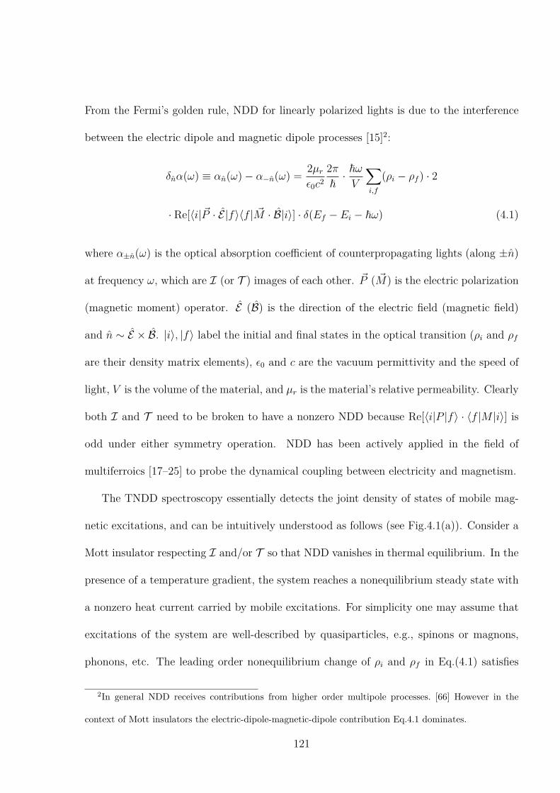
From the Fermi’s golden rule, NDD for linearly polarized lights is due to the interference
between the electric dipole and magnetic dipole processes [15]2:
δnα(ω) ≡ αn(ω)− α−n(ω) =2µr
ϵ0c22π
~· ~ωV
∑i,f
(ρi − ρf ) · 2
· Re[⟨i|P · E |f⟩⟨f |M · B|i⟩] · δ(Ef − Ei − ~ω) (4.1)
where α±n(ω) is the optical absorption coefficient of counterpropagating lights (along ±n)
at frequency ω, which are I (or T ) images of each other. P (M) is the electric polarization
(magnetic moment) operator. E (B) is the direction of the electric field (magnetic field)
and n ∼ E × B. |i⟩, |f⟩ label the initial and final states in the optical transition (ρi and ρf
are their density matrix elements), ϵ0 and c are the vacuum permittivity and the speed of
light, V is the volume of the material, and µr is the material’s relative permeability. Clearly
both I and T need to be broken to have a nonzero NDD because Re[⟨i|P |f⟩ · ⟨f |M |i⟩] is
odd under either symmetry operation. NDD has been actively applied in the field of
multiferroics [17–25] to probe the dynamical coupling between electricity and magnetism.
The TNDD spectroscopy essentially detects the joint density of states of mobile mag-
netic excitations, and can be intuitively understood as follows (see Fig.4.1(a)). Consider a
Mott insulator respecting I and/or T so that NDD vanishes in thermal equilibrium. In the
presence of a temperature gradient, the system reaches a nonequilibrium steady state with
a nonzero heat current carried by mobile excitations. For simplicity one may assume that
excitations of the system are well-described by quasiparticles, e.g., spinons or magnons,
phonons, etc. The leading order nonequilibrium change of ρi and ρf in Eq.(4.1) satisfies
2In general NDD receives contributions from higher order multipole processes. [66] However in the
context of Mott insulators the electric-dipole-magnetic-dipole contribution Eq.4.1 dominates.
121

δρi, δρf ∝ ∇T · τ from a simple Boltzmann equation analysis, where τ is the relaxation
time.
The crucial observation is that this nonequilibrium state breaks both the inversion
symmetry (by ∇T ) and the time-reversal symmetry (by τ). Consequently one expects
a NDD signal proportional to ∇T · τ . Precisely speaking TNDD is a second-order thermo-
electromagnetic nonlinear response: it is a change of optical absorption (a linear response)
due to a temperature gradient. The factor ∇T ·τ in TNDD indicates that it is a generaliza-
tion of Drude-phenomenon to nonlinear responses. Notice that the Drude-phenomenon is
independent of whether the system has a quasiparticle description or not. Even in the ab-
sence of quasiparticle descriptions, strongly interacting liquids may have nearly conserved
momentum. The relaxation time τ in Drude physics should be interpreted as the momen-
tum relaxation time [26]. This indicates that TNDD discussed here can be generalized to
systems without quasiparticle descriptions such as the U(1)-Dirac spin liquid [27–29] and
the spinon Fermi surface state [30, 31].
Advantages of TNDD spectroscopy Now we comment on the major advantages
of TNDD as a probe of spin dynamics. First, TNDD is a dynamical spectroscopy with
the frequency resolution in contrast to the DC thermal transport, and essentially probes
the joint density of states of magnetic excitations. Second, the fact that TNDD only
receives contributions from Re[⟨i|P |f⟩ · ⟨f |M |i⟩] dictates that the phonons’ contribution
can be safely ignored: The natural unit for the magnetic moment of phonon, the nuclear
magneton, is more than three orders of magnitudes smaller than that of the electron, the
Bohr magneton.
In addition, at the intuitive level, a local magnetic mode (e.g. from a magnetic impurity
122

atom) can only couple to a local temperature instead of a temperature gradient. A local
temperature respects both I (after taking disorder-average) and T . Consequently, such
local modes are not expected to contribute to TNDD either. From a more careful estimate
(see App.4.4.1 for detailed discussions), we find that the contribution to TNDD from local-
ized modes with a localization length ξ, comparing to the contribution from the intrinsic
mobile magnetic modes, is at least down by a factor of ξ/lm, where lm is the mean-free
path of the mobile magnetic excitations. We have assumed that ξ ≪ lm: for local magnetic
modes carried by magnetic impurity atoms or crystalline defects, typically ξ is comparable
with the lattice spacing a, while usually lm ≫ a in a reasonably clean Mott insulator at
low temperatures.
Estimate of the TNDD response One may estimate the size of TNDD signal in a
spin-orbital coupled Mott insulator. The relevant dimensionless ratio limiting the experi-
mental resolution is:
TNDD(ω) ≡ δnα(ω)
αn(ω) + α−n(ω). (4.2)
In a Mott insulator, the polarization carried by a magnetic excitation can be estimated
as ζ · e · a, where a is the lattice spacing and ζ is dimensionless. Assuming the average
temperature of the system kBT to be comparable to the magnetic excitation energy3, we
find that (see App.4.4.2 for details):
TNDD(ω) ∼(D
J
)2ζ
α· |∇T | · lm
T∼(D
J
)2
· |∇T | · lmT
, (4.3)
3Similar to a thermal transport experiment, if the temperature of the system is far below the magnetic
excitation energy, a temperature gradient would not efficiently affect the magnetic excitation distributions
and would not lead to a sizable TNDD.
123

in the limit of a weak spin-orbit coupling. Here α ≈ 1/137 is the fine-structure constant
and we used ζ ∼ 10−2 ∼ α in typical transition metal Mott insulators [33]. Notice that in
the absence of spin-orbit coupling, TNDD vanishes since the spin magnetic moment M is
a spin-triplet4. D and J are the Dzyaloshinskii-Moriya(DM) interaction and the exchange
interaction respectively. In a system with a strong spin-orbit coupling one may setD/J ∼ 1,
and TNDD(ω) is proportional to the ratio of the temperature change across lm and the
temperature. To optimize signal, one may choose a large temperature gradient such that
∇T · w ∼ T where w is the linear system size along the ∇T direction, and TNDD(ω) ∼
lm/w. For instance, lm of magnetic excitations in a quantum spin ice material was reported
to be of the order of a micron [35]. For a typical millimeter sample size, TNDD(ω) can be
as large as 10−3, well detectable within the currently available experimental technology.
Crystal symmetry analysis TNDD can be phenomenologically described by a tensor
η:
δnα(ω) =∑a,b,c
ηabc(ω)EaBb∇cT (4.4)
The symmetry condition for ηabc(ω) is determined by the fusion rule of two vectors (E ,∇T )
and one pseudovector (B) into a trivial representation under the point group. For any point
group, symmetry always allows nonzero ηabc: one may always consider the case n ∼ E × B
to be parallel to ∇T .
As an example, we find that there are four independent response coefficients for the D3d
4We only consider the contribution from the spin magnetic moment in this chapter. The orbital magnetic
moment in a Mott insulator is a spin-singlet but is much smaller than the spin magnetic moment, by a
factor of (t/U)2 in the (t/U)-expansion. [33,67]
124

point group:
δnα = η1∇zT (E × B)z + η2Bz(E × ∇T )z + η3Ez(B × ∇T )z
+ η4[(ExBy + EyBx)∇yT − (ExBx − EyBy)∇xT
](4.5)
Here the x-axis is a C2-axis and the yz-plane is a σd mirror-plane in the D3d group. The
D3d point group is realized in the QSL candidate Herbertsmithite, in the Heisenberg model
on the Kagome lattice with DM interactions (see below and Fig.4.1(b)), as well as in
the generalized Kitaev-Heisenberg model on the honeycomb lattice [36–38], relevant for
Na2IrO3 [39] and RuCl3 [40–42].
Microscopic model We present a concrete microscopic calculation for the TNDD
spectrum. The nearest neighbor spin-1/2 Hamiltonian under consideration is on the kagome
lattice:
H = J∑<ij>
Si · Sj +∑<ij>
Dij · Si × Sj, (4.6)
This model is relevant for various QSL candidate materials such as ZnCu3(OH)6Cl2 (Her-
bertsmithite) and Cu3Zn(OH)6FBr, and respects both T and I. Based on the D3d crystal
symmetry for the kagome plane, the DM vector Dij = −Dji has two independent coupling
constants: Dz (out-of-plane) and Dp (in-plane) [43] (see Fig.4.1(b)). Precisely speaking:
Dij = dij · (Dz · z +Dp · z × rij), (4.7)
where dij = ±1, rij is the unit vector along the direction from the site-j to the site-i. As
shown in Fig.4.1(b), in each bow-tie: d12 = d23 = d31 = 1, d34 = d45 = d53 = −1.
Dipole-coupling with an external electric field δH = −E · P , the electric polarization P
125
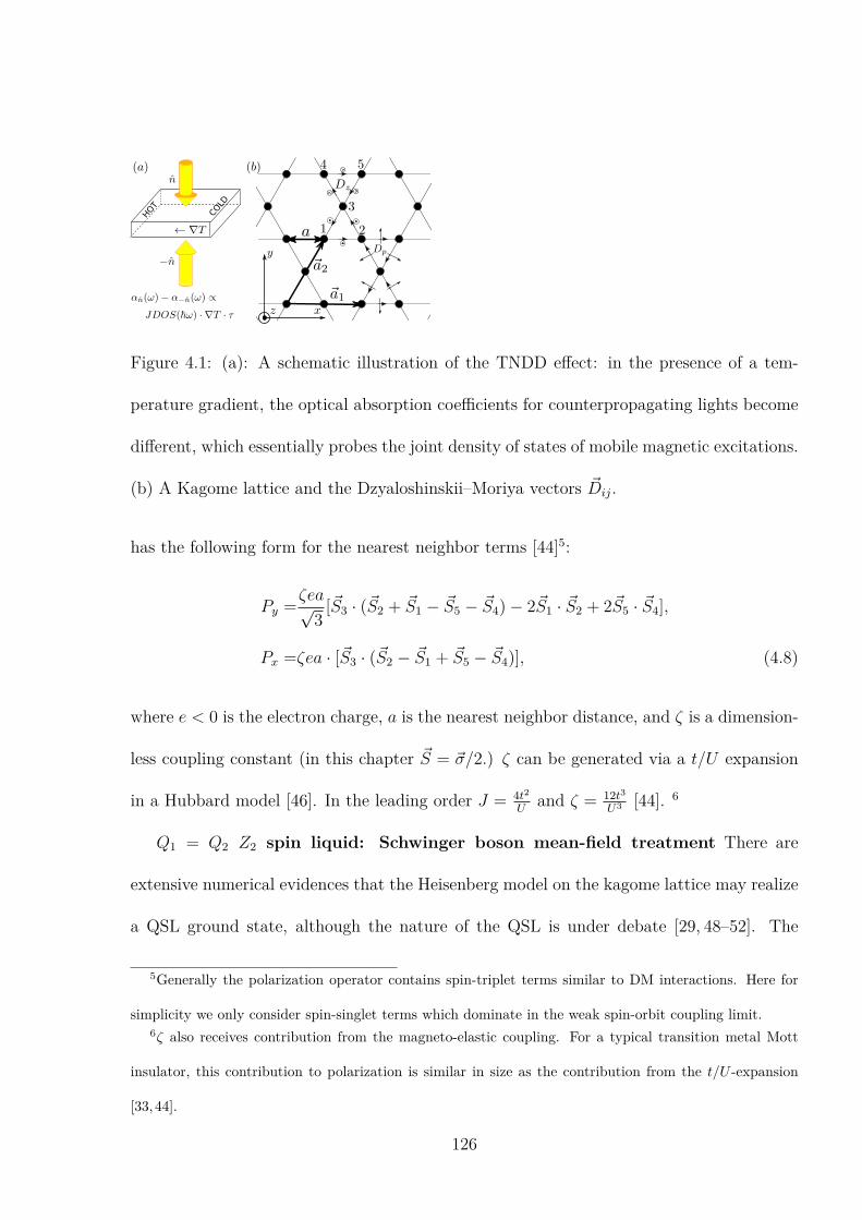
HOT
COLD
Figure 4.1: (a): A schematic illustration of the TNDD effect: in the presence of a tem-
perature gradient, the optical absorption coefficients for counterpropagating lights become
different, which essentially probes the joint density of states of mobile magnetic excitations.
(b) A Kagome lattice and the Dzyaloshinskii–Moriya vectors Dij.
has the following form for the nearest neighbor terms [44]5:
Py =ζea√3[S3 · (S2 + S1 − S5 − S4)− 2S1 · S2 + 2S5 · S4],
Px =ζea · [S3 · (S2 − S1 + S5 − S4)], (4.8)
where e < 0 is the electron charge, a is the nearest neighbor distance, and ζ is a dimension-
less coupling constant (in this chapter S = σ/2.) ζ can be generated via a t/U expansion
in a Hubbard model [46]. In the leading order J = 4t2
Uand ζ = 12t3
U3 [44]. 6
Q1 = Q2 Z2 spin liquid: Schwinger boson mean-field treatment There are
extensive numerical evidences that the Heisenberg model on the kagome lattice may realize
a QSL ground state, although the nature of the QSL is under debate [29, 48–52]. The
5Generally the polarization operator contains spin-triplet terms similar to DM interactions. Here for
simplicity we only consider spin-singlet terms which dominate in the weak spin-orbit coupling limit.6ζ also receives contribution from the magneto-elastic coupling. For a typical transition metal Mott
insulator, this contribution to polarization is similar in size as the contribution from the t/U -expansion
[33,44].
126

present work does not attempt to resolve this long-standing puzzle. Instead, we will focus
on one candidate spin liquid state, which may be realized in the model Eq.(4.6): Sachdev’s
Q1 = Q2 Z2 QSL [53]. The Q1 = Q2 QSL is a gapped state and can be described using the
Schwinger boson mean-field theory [54–56], in which spin is represented by bosonic spinons:
Si =12b†iασαβbiβ, while boson number per site is subject to the constraint b†iαbiα = 2S. We
then do the usual mean-field decoupling and diagonalize the quadratic mean-field spinon
Hamiltonian to obtain three spinon bands. We treat DM interaction as a perturbation and
keep contributions up to the linear order of D/J . Under this approximation we arrive at
the following mean-field Hamiltonian.
HMF = −µ∑i
(b†iαbiα − 2S)− J
2
∑⟨ij⟩
(A∗ijAij + h.c.)
+∑⟨ij⟩
(Dij
4· Aij
ˆC†
ij + h.c.), (4.9)
where operators Aij ≡ biαϵαβbjβ and Cij ≡ −ibiα(ϵσ)αβbjβ. HMF may be viewed as an ansatz
to construct variational spin-liquid wavefunctions with parameters Aij, µ. In Sachdev’s
Q1 = Q2 state, Aij have the following spatial pattern: Aij = dijA, and A can be chosen to
be real. See Appendix. 4.4.3 for more details.
After Bogoliubov diagonalization, three bands are found: HMF =∑α=↑,↓
k,u=1,2,3Eu,kγ
α†u,kγαu,k
as shown in Fig.4.2, where ↑, ↓ label the Kramers degeneracy. Tuning chemical potential
µ so that the band structure is near the boson condensation at Γ, the lowest energy band
u = 1 is well described by a relativistic boson disperson:
E1,k ≈√∆2 + ~2k2v2, (4.10)
where ∆ is the bosonic spinon gap.
127

- 2 - 1 0 1 2
0.0
0.5
1.0
1.5
Figure 4.2: The Schwinger boson band dispersion (blue solid lines) for the mean-field
Hamiltonian Eq.(4.9) of Sachdev’s Q1 = Q2 Z2 QSL with parameters A = 1, Dz = Dp =
0.1J , and µ = −1.792J . The low energy band-1 near the Γ point is well described by
the relativistic dispersion Eq.(4.10) with gap ∆ = 0.16J (red line). The two-spinon (red
dots at ±k) contribution to the TNDD response computed in Eq.(4.11) and App.4.4.3 is
illustrated.
TNDD contributed from the bosonic spinons In the low temperature limit, the
two-spinon contribution dominates TNDD with |f⟩ ∼ γα,†u,kγβ†v,−k
|i⟩ in Eq.(4.1). 7. ρi, ρf in
Eq.(4.1) is related to the nonequilibrium bosonic spinon occupation gu,k. From a simple
Boltzmann equation analysis with a single relaxation time τ , gu,k deviates from the equilib-
rium occupation g0u,k
= 1
eβ(r)E
u,k−1by δgu,k =
∂g0u,k
(r)
∂EEu,k
τ vu,k
·∇T
T (r), where vu,k =
∂Eu,k
~∂k. This
δgu,k is responsible for TNDD.
Since TNDD is a bulk response we consider a 3D system consisting of stacked 2D layers
each described by the model Eq.(4.6) with an interlayer distance d. Using the electric
polarization Eq.(4.8) and spin magnetic moment M = gsµBS, in App.(4.4.3 we compute
the low temperature/energy TNDD response tensor defined in Eq.(4.4) within our mean-
7Notice that a single spinon excitation is not gauge invariant and does not contribute to physical
responses
128

2Δ 4Δ
0
2
4
6
0
2
4
6
Figure 4.3: The bosonic two-spinon contribution to TNDD spectra of Sachdev’s Q1 = Q2
Z2 QSL Eq.(4.9) at the temperature kBT = 0.7∆ (solid black line) and kBT = 0.4∆ (solid
red line), together with the two-spinon joint density of states (dashed blue line).
field treatment (corresponding to η2 in Eq.(4.5)). As plotted in Fig.4.3, we find that
(x, y, z-directions are illustrated in Fig.4.1)
ηxzy(ω) = C ·[1 + 2g0(~ω/2)
]· (kBT )3
·[3G3(z)− 3lnz ·G2(z) + (lnz)2G1(z)
]· e−
√(~ω/2)2−∆2/∆ · ~ω · JDOS(~ω) · τ · v
T. (4.11)
Here the constant C ≡ 8πu0α2ζaa0 · µrgsa3
~3v3 , where a0 is the Bohr radius. u0 ∝ (D/J)2 is
a dimensionless constant related to the mean-field band structure and can be determined
numerically. For the parameters Dz = Dp = 0.1J and µ = −1.792J we find that u0 =
0.603. The 3D optical joint density of states JDOS(~ω) ≡ D · ~ω · Θ(~ω − 2∆) where
D ≡ 18π~2v2d . g0(~ω/2) = 1
eℏω/2kBT−1, z ≡ e
− ∆kBT , and Gν(z) ≡ 1
Γ(ν)
∫∞0
xν−1dxz−1ex−1
is the Bose-
Einstein integral. Eq.(4.11) holds when the temperature and the photon energy are within
the regime of the relativistic dispersion Eq.(4.10).
In the limit kBT ≪ ∆, Eq.(4.11) can be simplified and we have ηxzy(ω) ∝ e−∆/kBT ,
where the thermal activation factor can be traced back to δgk. Importantly, beyond the
mean-field treatment, TNDD is generally ∝ δρi, δρf ∝ ∇T · τ in Eq.(4.1), and a thermal
129

activation factor e−∆/kBT in TNDD is always due to the energy diffusion near the mobility
gap ∆. Therefore TNDD can serve as a sharp measurement of the mobility gap ∆ of the
magnetic excitations.
4.3 Discussion and conclusion
Bosonic vs. fermionic spinons We computed the TNDD response contributed from bosonic
spinons in the Sachdev’s Q1 = Q2 Z2 QSL. Fermionic spinons also exist in this Z2 QSL
and their contribution to TNDD can be similarly computed in a dual Abrikosov fermion
approach [58,59]. Without pursuing this calculation in details, one expects that the bosonic
factor [1 + 2g0(~ω/2)] (Bose-Einstein integrals) in Eq.(4.11) will be replaced by the cor-
responding fermionic factor [1 − 2f 0(~ω/2)] (Fermi-Dirac integrals), where f 0(~ω/2) =
1/(e~ω/2kBT + 1). The contributions from the bosonic spinons and fermionic spinons have
different temperature dependence, which, in principle, may be used to detect the statistics
of quasiparticles in certain situations.
Magnetically ordered states It is also interesting to consider the TNDD response in a
conventional magnetically ordered state respecting either I, or T combined with a lattice-
translation symmetry (as in the case of an antiferromagnet), or both. One may similarly
consider the two-magnon contribution to the TNDD response, which probes the joint den-
sity of states of magnons. Our estimate Eq.(4.3) will be modified as follows (see Appendix
4.4.2 for details). If the magnetic order is non-collinear, which breaks spin-rotational sym-
metry completely, the (D/J)2 factor in Eq.(4.3) is replaced by ∼ 1. If the magnetic order
is collinear, which only breaks the spin-rotation symmetry down to U(1), the (D/J)2 factor
130

is replaced by D/J .
Conclusion In this chapter we propose the temperature-gradient-induced nonrecipro-
cal directional dichroism (TNDD) spectroscopy experiment in Mott insulators. Comparing
with traditional probes for magnetic excitations, TNND spectroscopy has unique advan-
tages: it directly probes mobile magnetic excitations and decouples from local impurity
modes and phonon modes. For instance, an activation behavior ∝ e−∆/kBT in the tempera-
ture dependence of TNDD sharply measures the mobility gap ∆ of the magnetic excitations,
a quantity challenging to measure using traditional probes but of fundamental importance
in the field of topologically ordered QSL.
The present work can be viewed as one example in a large category of nonlinear thermo-
electromagnetic responses. There are other interesting effects. For instance, a temperature
gradient also induces a circular dichroism in a system respecting both T and I. We leave
these other responses as topics of future studies.
4.4 Appendices
4.4.1 Localized modes
Let us consider the situation of a Mott insulator in the presence of impurities/disorders,
which could introduce localized magnetic modes. Below we consider the contribution to
TNDD response from these localized modes.
Firstly, we comment on the meaning of “localized modes” discussed here. In an isolated
localized phase of matter, like a many-body localized phase(see Ref. [60, 61] for reviews),
thermalization breaks down and the meaning of a temperature-gradient is unclear. We are
131

NOT discussing the TNDD response in this situation.
In realistic quantum materials, the magnetic localized modes are coupled with a thermal
bath (e.g., phonon thermal bath) and a local temperature is well defined. To facilitate the
discussion, one may consider a system with a U(1) spin rotation symmetry in order to
sharply define a magnetic localized mode. In addition, we assume a finite mobility gap ∆
of the U(1) charge, and magnetic localized excitations may exist below ∆. Assuming lm
being the mean-free path for mobile magnetic excitations, practically the localized magnetic
modes may fall into two regimes according to the localization length ξ:
(1): ξ ≪ lm. This is the more common situation realized in practical materials. Here
the localized magnetic modes may be extrinsic magnetic impurity atoms, or may form at
crystalline defects. They may also form at the centers of the vortices of valence bond solid
(VBS) order [62]. Typically the localization length ξ of these magnetic modes is of the
same order as the lattice spacing a, while lm ≫ a in a reasonably clean Mott insulator.
It is difficult to model a magnetic localized mode with ξ ∼ a since lattice scale details
cannot be neglected. Instead, we consider the following situation a ≪ ξ ≪ lm so that a
low energy effective description is still valid. As a crude model for such magnetic localized
modes, one may consider a quantum dot of size ξ in the presence of a temperature gradient;
for instance, the left (right) edge of the quantum dot is in contact with a heat reservior
at temperature TL (TR). The modes in the quantum dot are travelling ballistically since
ξ ≪ lm. Consequently the right-mover (left-mover) in the quantum dot is at temperature
TL (TR). Such a nonequilibrium ensemble is quantitatively comparable with a large (energy-
)diffusive system in the presence of the same temperature gradient but with lm ∼ ξ (for
example, see Eq.(4.24)). Namely, in the present situation, ξ replaces the role of lm in our
132
estimate Eq.(4.3). we conclude that the dimensionless ration TNDD(ω) contributed by
such localized modes is reduced by a factor of ∼ ξ/lm.
(2): ξ ≫ lm. In this situation, the system hosts would-be mobile modes. These modes
scatter with disorder multiple times before eventually become localized. For instance,
Anderson weak-localization in two spatial dimensions happens with ξ parametrically larger
than lm. It is instructive to consider a system size L satisfying ξ > L > lm. For such a
system size the localization physics is not present yet. Because photon absorption is still a
local process, we expect that the contribution to the TNDD response from such localized
modes to be comparable with that from mobile modes.
In summary, the contribution to TNDD response from localized modes in the regime
ξ ≪ lm can be safely neglected. In the opposite regime ξ ≫ lm, the localized modes still
contribute to TNDD significantly. Nevertheless, the localized modes in the latter regime
are would-be extended (mobile) states in the absence of disorder.
4.4.2 Spin-orbit coupling and the estimate of TNDD response
From the discussion in the main text and Eq.(4.1), up to matrix element effects, the TNDD
spectroscopy directly probes the joint density of states JDOS(~ω) of the mobile magnetic
excitations:
δnα(ω) ≡ αn(ω)− α−n(ω) ∝ ~ω · JDOS(~ω) · ∇T · τ (4.12)
In order to estimate the optical absorption coeffient αn in a Mott insulator, one need to
estimate the strength of electric polarization and the magnetic dipole moment. It turns out
that they are comparable in a typical transition metal Mott insulator, which is drastically
different from the case of a band metal/insulator. In the latter case the electric polarization
133
carried by a typical particle-hole excitation is ∼ e · a where e is the electron charge and
a is the lattice constant, while the magnetic moment carried by the same excitation is of
the order of a Bohr magneton µB. For a given electromagnetic wave, the magnetic dipole
energy scale µB · B is smaller than the electric dipole energy scale e · a · E by roughly a
factor of the fine-structure constant ∼ 1/137, which is why the magnetic dipole processes
are often neglected in a band metal/insulator.
In a Mott insulator, however, the electric polarization carried by a magnetic excitation
is heavily reduced. In the framework of the Hubbard model, this electric polarization can
be estimated as ζ ·e ·a where the dimensionless factor ζ ∼ 8(t/U)3 [33]. On the other hand,
the magnetic dipole moment carried by the same excitation is still ∼ µB. As a result, they
would have comparable sizes for typical 3d transition metal Mott insulators with t/U ∼ 10.
The absorption coefficient due to the electric dipole processes can be estimated based
on the Fermi’s golden rule:
αn(ω) ∼2
nrϵ0c
2π
~· |⟨f |P |i⟩|2 · ~ω · JDOS(~ω)
∼ 16π2
nr
αζ2a2 · ~ω · JDOS(~ω). (4.13)
where nr is the relative refractive index of the material, c is the speed of light, α is the
fine structure constant ∼ 1/137, and JDOS(~ω) is the joint density of states for the
relevant excitations at photon energy ~ω. We assume that the temperature is comparable
with the magnetic excitation energy scale, and we have used the typical matrix element
⟨f |P |i⟩ ∼ ζ · e · a where a is the lattice constant.
Notice that JDOS(~ω) may be estimated as ∼ 1a3
1W
where a is the lattice constant
and W is the band width of the excitations. For a typical photon energy ∼ W , one finds
134

that ~ω · JDOS(~ω) ∼ 1/a3, independent of the nature of the excitations. For instance,
the interband absorption coefficient α(ω) in a band metal/insulator is typically ∼ 107m−1.
The dimensionless coupling constant ζ reduces by a factor of 102 in transition metal Mott
insultors, which gives the absorption coefficient ∼ 103m−1, broadly consistent with the
tera-Hertz penetration depth (∼ 1mm) for these quantum magnets [63, 64].
The TNDD response can be similarly estimated. We first consider the case of a quantum
paramagnet.
δnα(ω) ∼2µr
ϵ0c22π
~· (ρi − ρf ) · 2 · Re[⟨f |P |i⟩⟨i|M |f⟩]
· ~ω · JDOS(~ω) (4.14)
We again assume that the temperature is comparable with the magnetic excitation energy
scale, and consequently the effect of temperature gradient in (ρi − ρf ) can be estimated by
the dimensionless factor |∇T |·lmT
where lm is the mean-free path of the magnetic excitations.
If the spin-orbit coupling (SOC) is strong one may estimate ⟨f |P |i⟩ ∼ ζea while ⟨i|M |f⟩ ∼
gsµB (gs is the g-factor the spin magnetic moment.). Putting together we have:
δnα(ω) ∼ 16π2µrgsα2ζa0a ·
|∇T | · lmT
· ~ω · JDOS(~ω),
if strong SOC. (4.15)
Here a0 is the Bohr radius.
From Eq.(4.13,4.15), and a0 ∼ a, we can estimate that if the spin-orbit coupling is
strong and the temperature is comparable with the magnetic excitation energy scale, the
dimensionles ratio TNDD in Eq.(4.2)
TNDD(ω) ∼ α
ζ
|∇T | · lmT
∼ |∇T | · lmT
, if strong SOC. (4.16)
135

Here we used the fact that for a typical transition metal Mott insulator ζ ∼ 10−2 ∼ α.
In the absence of the SOC, ⟨i|M |f⟩ = 0 because M = gsµBS is proportional to the
conserved total spin S (We only consider the spin magnetic moment. The orbital magnetic
moment in Mott insulators is much smaller and neglected.). In the limit of a weak SOC:
D/J ≪ 1, the TNDD response can be estimated as follows. The only effect of the weak
SOC is in the matrix element product: ⟨f |P |i⟩⟨i|M |f⟩.
For the magnetic dipole matrix element: ⟨i|M |f⟩ ∝ 1Ef−Ei
⟨i|[S,H]|f⟩ ∝ ⟨f |D · [S, Si ×
Sj]|i⟩. Notice that the operator of the commutator is a spin triplet. There are two possi-
bilities: (1): the states |f⟩ and |i⟩ differ by spin-1 in the limit D/J → 0. For instance, |f⟩
may be a spin triplet while |i⟩ is a spin singlet in that limit; (2): the states |f⟩ and |i⟩ have
the same spin in the limit D/J → 0.
In the situation-(2), the magnetic dipole matrix element ⟨i|M |f⟩ ∝ (D/J)2, because
the wavefunction corrections of |f⟩ and |i⟩ due to nonzero D/J need to be considered. In
this situation, the electric dipole matrix element ⟨f |P |i⟩ ∝ (D/J)0 since P is a spin singlet
operator in the limit of D/J → 0. Therefore in situation-(2) we have ⟨f |P |i⟩⟨i|M |f⟩ ∝
(D/J)2.
In the situation-(1), a similar consideration leads to: ⟨i|M |f⟩ ∝ (D/J) and ⟨f |P |i⟩ ∝
(D/J). So we still have ⟨f |P |i⟩⟨i|M |f⟩ ∝ (D/J)2.
In summary, we have the following estimate in a quantum paramagnet assuming the
temperature is comparable with the magnetic excitation energy scale:
TNDD(ω) ∼(D
J
)2α
ζ
|∇T | · lmT
∼(D
J
)2 |∇T | · lmT
, if weak SOC. (4.17)
136

Next we estimate the TNDD response in magnetic ordered states due to magnon excita-
tions. Even in the absence of microscopic SOC, the (D/J)2 factor in the estimate Eq.(4.17)
will be replaced by ∼ 1 in a non-collinear magnetic ordered state, because the spin-rotation
symmetry is completely broken.
In a collinear magnetic ordered state, the spin rotation symmetry is broken down to U(1)
in the absence of SOC. The electric polarization operator P is expected to carry zero charge
under this U(1) rotation. To have a nonzero matrix element product ⟨f |P |i⟩⟨i|M |f⟩, one
must consider the linear-order effect of the SOC. Therefore in this case the (D/J)2 factor
in the estimate Eq.(4.17) will be replaced by ∼ D/J .
4.4.3 Details of the mean-field calculation for TNDD
In this section we provide a detailed account of the Schwinger boson mean-field theory.
The spin is represented by bosonic spinons
Si =1
2b†iασαβbiβ, (4.18)
while boson number per site is subject to the constraint:
b†iαbiα = κ. (4.19)
Although κ = 2S for spin-S, it will be convenient to consider κ to be a continuous param-
eter, taking on any non-negative value [53, 65].
Considering the operator identities Si ·Sj = −12A†
ijAij+κ2
4and Si×Sj =
14[ˆC†
ijAij+h.c.],
where
Aij = −Aji = biαϵαβbjβ,ˆCij =
ˆCji = −ibiα(ϵσ)αβbjβ. (4.20)
137
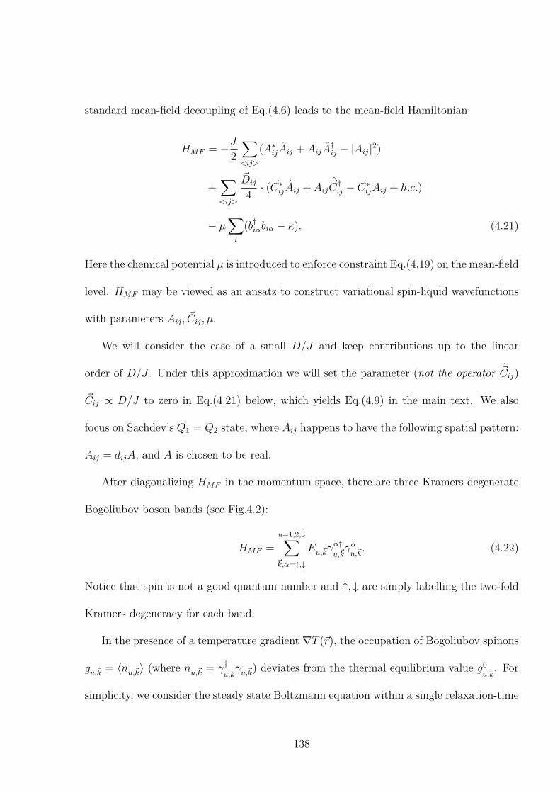
standard mean-field decoupling of Eq.(4.6) leads to the mean-field Hamiltonian:
HMF = −J2
∑<ij>
(A∗ijAij + AijA
†ij − |Aij|2)
+∑<ij>
Dij
4· (C∗
ijAij + AijˆC†
ij − C∗ijAij + h.c.)
− µ∑i
(b†iαbiα − κ). (4.21)
Here the chemical potential µ is introduced to enforce constraint Eq.(4.19) on the mean-field
level. HMF may be viewed as an ansatz to construct variational spin-liquid wavefunctions
with parameters Aij, Cij, µ.
We will consider the case of a small D/J and keep contributions up to the linear
order of D/J . Under this approximation we will set the parameter (not the operator ˆCij)
Cij ∝ D/J to zero in Eq.(4.21) below, which yields Eq.(4.9) in the main text. We also
focus on Sachdev’s Q1 = Q2 state, where Aij happens to have the following spatial pattern:
Aij = dijA, and A is chosen to be real.
After diagonalizing HMF in the momentum space, there are three Kramers degenerate
Bogoliubov boson bands (see Fig.4.2):
HMF =
u=1,2,3∑k,α=↑,↓
Eu,kγα†u,kγαu,k. (4.22)
Notice that spin is not a good quantum number and ↑, ↓ are simply labelling the two-fold
Kramers degeneracy for each band.
In the presence of a temperature gradient ∇T (r), the occupation of Bogoliubov spinons
gu,k = ⟨nu,k⟩ (where nu,k = γ†u,kγu,k) deviates from the thermal equilibrium value g0
u,k. For
simplicity, we consider the steady state Boltzmann equation within a single relaxation-time
138

approximation:
vu,k · ∇rgu,k(r) = −gu,k(r)− g0
u,k(r)
τ, (4.23)
where g0u,k
(r) = 1
eEu,k
/kBT (r)+1
, vu,k = 1~∇kEu,k. To the leading order, these give δgu,k(r) ≡
gu,k(r)− g0u,k
(r):
δgu,k(r) ≡ δg↑u,k
(r) = δg↓u,k
(r) =∂g0
u,k(r)
∂EEu,k
τ vu,k · ∇TT (r)
(4.24)
Since the velocity vu,k = −vu,−k, we have:
δgu,k(r) = −δgu,−k(r) (4.25)
To be concrete, we focus on the case E = x and B = z, with the light propagating
direction n = −y and the temperature gradient ∇T ∝ y(the η2 response in Eq.(4.5)). In
order to compute the matrix elements in Eq.(4.1), one writes Px and Mz in terms of the
Bogoliubov bosons, and selects the relevant terms:
Px →v,α,w,α′∑
q
Xv,α,w,α′
q γα†v,qγα′†w,−q + h.c.
+1
A
v,α,w,α′,t,β∑q,p
Y v,α,w,α′,t,βq,p γα†v,qγ
α′†w,−qγ
β†t,pγ
βt,p + h.c.,
Mz = −gsµb
∑i
b†iασzαβ
2biβ
→v,α,w,α′∑
q
Zv,α,w,α′
q γα†v,qγα′†w,−q + h.c.. (4.26)
The objects Xv,α,w,α′
q , Y v,α,w,α′,t,βq,p , Zv,α,w,α′
q are determined by the Bogoliubov transforma-
tion from Eq.(4.9) to Eq.(4.22).
Plugging in Eq.(4.1), one finds
δnα(ω) =8πµr
ϵ0c2dRe[I(ω)], (4.27)
139

where
I(ω) =ω
A
v,α,w,α′∑q
[Xv,α,w,α′
q +1
A
t,β∑p
Y v,α,w,α′,t,βq,p · gt,p
]∗· Zv,α,w,α′
q (1 + gv,q + gw,−q) · δ(Ev,q + Ew,−q − ~ω). (4.28)
Here the bosonic factor (1 + gv,q + gw,−q) is well anticipated from the golden rule. The
factor gt,p appears because of the quartic interactions in P in Eq.(4.8).
It is a good moment to study the symmetry property of I(ω). In thermal equilibrium,
it is straightforward to see that the inversion symmetry alone dictates I(ω) = 0, while
time-reversal symmetry alone allows a nonzero imaginary part of I(ω) (giving rise to the
well-known natural circular dichroism in noncentrosymmetric systems).
Next we consider the effect of nonequilibrium occupation δgu,k in Eq.(4.24). Expanding
Eq.(4.28) gives three contributions, I = I(A) + I(B) + I(C):
I(A)(ω) ∝ X∗ · Z · (δgv,q + δgw,−q),
I(B)(ω) ∝ Y ∗ · Z · g0t,p · (δgv,q + δgw,−q),
I(C)(ω) ∝ Y ∗ · Z · δgt,p · (1 + g0v,q + g0w,−q). (4.29)
While the inversion symmetry allows all these contributions, the time-reversal symmetry
only allows their real parts: the directional dichroism. In addition, in the special situation
that v = w, namely if the created two spinons are in the same band, obviously I(A)(ω) =
I(B)(ω) = 0 due to Eq.(4.25) and only I(C)(ω) is nonzero.
Focusing on the low temperature/energy TNDD spectroscopy, one may consider the
contribution v = w = t = 1 from the lowest energy band only (see Fig.4.2 for a plot of the
140

Figure 4.4: The fit log(Wq,p/[py · (ζea4gsµB)]) = log(u0) −√E2
1,q −∆2/∆ (i.e., Eq.(4.31)
with u = uy = u0ζea4gsµB y) with only one fitting parameter u0. In each case 696 data
points with both√E2
1,p −∆2/∆ and√E2
1,q −∆2/∆ between 0.5 and 1.7 are plotted. Since
many data points are related by the lattice symmetry and/or share the same momentum
q (but different p), the visibly different data points are much fewer. We set A = 1,
and consider three cases of different SOC strength: case-(a): Dz = Dp = 0.025J (and
µ = −1.752J); case-(b): Dz = Dp = 0.05J (and µ = −1.765J); case-(c) Dz = Dp = 0.1J
(and µ = −1.792J). Notice that for each case the chemical potential µ is tuned so that
the spinon gap is fixed to be ∆ = 0.16J . As shown in this figure, we numerically find that
u0 = 0.0378 in case-(a), u0 = 0.151 = 0.0378·3.99 in case-(b), and u0 = 0.603 = 0.151·3.99
in case-(c). The scaling u0 ∝ (D/J)2 is confirmed.
141

band structure), and compute I(ω) = I(C)(ω) analytically. In this case:
I(C)(ω) =ω
A2
∑q,p
Wq,p · δg1,p(1 + 2g01,q)δ(2E1,q − ~ω),
where Wq,p ≡∑α,α′,β
(Y 1,α,1,α′,1,βq,p )∗ · Z1,α,1,α′
q . (4.30)
Wq,p is a real function satisfying Wq,p = −W−q,−p due to the inversion symmetry. Taylor
expanding near the Γ-point, to the leading order one expects: Wq,p ≈ u · p+ v · q. In fact,
interestingly, we numerically found that Wq,p can be well described as
Wq,p = (u · p) e−√
E21,q
−∆2/∆ (4.31)
in the momentum regime where the relativistic dispersion Eq.(4.10) holds (see Fig.4.4 for
details). We do not attempt to analytically justify Eq.(4.31) here since it deviates from the
main purpose of this chapter. Eq.(4.30,4.31) then lead to:
I(C)(ω) =ω
A2
∑p
(u · p δg1,p)
·∑q
e−√
E21,q
−∆2/∆(1 + 2g01,q)δ(2E1,q − ~ω). (4.32)
Crystal symmetry and dimensional analysis show that u = uy = u0ζea4gsµB y, consistent
with the η2 response in Eq.(4.5). The dimensionless number u0 is expect to be ∼ (D/J)2
and can be determined numerically (see Fig.4.4 for details).
With Eq.(4.24,4.27,4.10,4.32) the low temperature/energy TNDD response can be com-
puted within our mean-field treatment:
δyα(ω) = C ·[1 + 2g0(~ω/2)
]· (kBT )3
·[3G3(z)− 3lnz ·G2(z) + (lnz)2G1(z)
]· e−
√(~ω/2)2−∆2/∆ · ~ω · JDOS(~ω) · ∇yT · τ · v
T. (4.33)
142

This is just the Eq.(4.11) in the main text.
We can apply the estimate in the previous section to the present example as follows.
We firstly estimate αn due to the electric dipole processes following the golden rule:
αn(ω) ∼2
nrϵ0c
2π
~(ζea)2[1 + 2g0(~ω/2)]~ω · JDOS(~ω)
=16π2
nr
αζ2a2[1 + 2g0(~ω/2)]~ω · JDOS(~ω), (4.34)
where nr is material’s relative refractive index. For the situation with kBT ∼ J ∼ ~va
and
~ω ∼ 2∆, Eq.(4.11,4.34) give the dimensionless ratio TNDD(ω) in Eq.(4.2):
TNDD(ω) ∼ αa0ζa
· u0∇yT · τ · v
T, (4.35)
confirming the estimate Eq.(4.3) since u0 ∝ (D/J)2.
Finally, we would like to remark on the validity of the mean-field treatment. Although
we performed the calculation within the mean-field approach, the main component of the
calculation (Eq.(4.29,4.30) in App.4.4.3) is justified as long as the quasiparticle description
is valid. These microscopic contributions to TNDD can be written down phenomenologi-
cally as a low quasiparticle-density expansion, up to the second order ∝ gp · gq. Some other
components of the calculation (e.g., the matrix element behavior Eq.(4.31) ) may receive
corrections moving beyond the mean-field approximation, but these would not change the
result of TNDD response qualitatively.
143

Bibliography
[1] P. Anderson, Materials Research Bulletin 8, 153 (1973).
[2] P. A. Lee, Journal of Physics: Conference Series 529, 012001 (2014).
[3] Y. Zhou, K. Kanoda, and T.-K. Ng, Rev. Mod. Phys. 89, 025003 (2017).
[4] L. Savary and L. Balents, Reports on Progress in Physics 80, 016502 (2016).
[5] C. Broholm, R. J. Cava, S. A. Kivelson, D. G. Nocera, M. R. Norman, and T. Senthil,
Science 367 (2020), 10.1126/science.aay0668,
[6] X.-G. Wen, Phys. Rev. B 65, 165113 (2002).
[7] X.-G. Wen, Rev. Mod. Phys. 89, 041004 (2017).
[8] M. P. Shores, E. A. Nytko, B. M. Bartlett, and D. G. Nocera, Journal of the American
Chemical Society 127, 13462 (2005),
[9] M. R. Norman, Rev. Mod. Phys. 88, 041002 (2016).
[10] Y. Kasahara, T. Ohnishi, Y. Mizukami, O. Tanaka, S. Ma, K. Sugii, N. Kurita, H.
Tanaka, J. Nasu, Y. Motome, T. Shibauchi, and Y. Matsuda, Nature 559, 227 (2018).
[11] M. Hermele, M. P. A. Fisher, and L. Balents, Phys. Rev. B 69, 064404 (2004).
144

[12] M. J. P. Gingras and P. A. McClarty, Reports on Progress in Physics 77, 056501
(2014).
[13] Or time-reversal symmetry combined with a spatial translation such as in an antifer-
romagnet
[14] R. Fuchs, The Philosophical Magazine: A Journal of Theoretical Experimental and
Applied Physics 11, 647 (1965), https://doi.org/10.1080/14786436508224252.
[15] D. Szaller, S. Bord´acs, V. Kocsis, T. R˜o om, U. Nagel, and I. K´ezsm´arki, Phys.
Rev. B 89, 184419 (2014).
[16] In general NDD receives contributions from higher order multipole processes. [66] How-
ever in the context of Mott insulators the electric-dipole-magnetic-dipole contribution
Eq.4.1 dominates.
[17] J. Goulon, A. Rogalev, C. Goulon-Ginet, G. Benayoun, L. Paolasini, C. Brouder, C.
Malgrange, and P. A. Metcalf, Phys. Rev. Lett. 85, 4385 (2000).
[18] M. Kubota, T. Arima, Y. Kaneko, J. P. He, X. Z. Yu, and Y. Tokura, Phys. Rev. Lett.
92, 137401 (2004).
[19] T. Arima, Journal of Physics: Condensed Matter 20, 434211 (2008).
[20] I. K´ezsm´arki, N. Kida, H. Murakawa, S. Bord´acs, Y. Onose, and Y. Tokura, Phys.
Rev. Lett. 106, 057403 (2011).
[21] Y. Takahashi, R. Shimano, Y. Kaneko, H. Murakawa, and Y. Tokura, Nature Physics
8, 121 (2012).
145

[22] Y. Okamura, F. Kagawa, M. Mochizuki, M. Kubota, S. Seki, S. Ishiwata, M. Kawasaki,
Y. Onose, and Y. Tokura, Nature Communications 4, 2391 (2013).
[23] I. Kzsmrki, D. Szaller, S. Bordcs, V. Kocsis, Y. Tokunaga, Y. Taguchi, H. Murakawa,
Y. Tokura, H. Engelkamp, T. Rm, and U. Nagel, Nature Communications 5, 3203
(2014).
[24] S. Toyoda, N. Abe, S. Kimura, Y. H. Matsuda, T. Nomura, A. Ikeda, S. Takeyama,
and T. Arima, Phys. Rev. Lett. 115, 267207 (2015).
[25] Y. Tokura and N. Nagaosa, Nature Communications 9, 3740 (2018).
[26] P. Jung and A. Rosch, Phys. Rev. B 75, 245104 (2007).
[27] I. Affleck and J. B. Marston, Phys. Rev. B 37, 3774 (1988).
[28] M. Hermele, T. Senthil, M. P. A. Fisher, P. A. Lee, N. Nagaosa, and X.-G. Wen, Phys.
Rev. B 70, 214437 (2004).
[29] Y. Ran, M. Hermele, P. A. Lee, and X.-G. Wen, Phys. Rev. Lett. 98, 117205 (2007).
[30] O. I. Motrunich, Phys. Rev. B 72, 045105 (2005).
[31] S.-S. Lee and P. A. Lee, Phys. Rev. Lett. 95, 036403 (2005).
[32] Similar to a thermal transport experiment, if the temperature of the system is far
below the magnetic excitation energy, a temperature gradient would not efficiently
affect the magnetic excitation distributions and would not lead to a sizable TNDD.
[33] L. N. Bulaevskii, C. D. Batista, M. V. Mostovoy, and D. I. Khomskii, Phys. Rev. B
78, 024402 (2008).
146

[34] We only consider the contribution from the spin magnetic moment in this chapter.
The orbital magnetic moment in a Mott insulator is a spin-singlet but is much smaller
than the spin magnetic moment, by a factor of (t/U)2 in the (t/U)-expansion. [33,67]
[35] Y. Tokiwa, T. Yamashita, D. Terazawa, K. Kimura, Y. Kasahara, T. Onishi, Y. Kato,
M. Halim, P. Gegenwart, T. Shibauchi, S. Nakatsuji, E.-G. Moon, and Y. Matsuda,
Journal of the Physical Society of Japan 87, 064702 (2018).
[36] G. Jackeli and G. Khaliullin, Phys. Rev. Lett. 102, 017205 (2009).
[37] J. c. v. Chaloupka, G. Jackeli, and G. Khaliullin, Phys. Rev. Lett. 105, 027204 (2010).
[38] H. Takagi, T. Takayama, G. Jackeli, G. Khaliullin, and S. E. Nagler, Nature Reviews
Physics 1, 264 (2019).
[39] Y. Singh and P. Gegenwart, Phys. Rev. B 82, 064412 (2010).
[40] J. A. Sears, M. Songvilay, K. W. Plumb, J. P. Clancy, Y. Qiu, Y. Zhao, D. Parshall,
and Y.-J. Kim, Phys. Rev. B 91, 144420 (2015).
[41] R. D. Johnson, S. C. Williams, A. A. Haghighirad, J. Singleton, V. Zapf, P. Manuel,
I. I. Mazin, Y. Li, H. O. Jeschke, R. Valent´ı, and R. Coldea, Phys. Rev. B 92, 235119
(2015).
[42] H. B. Cao, A. Banerjee, J.-Q. Yan, C. A. Bridges, M. D. Lumsden, D. G. Mandrus, D.
A. Tennant, B. C. Chakoumakos, and S. E. Nagler, Phys. Rev. B 93, 134423 (2016).
[43] M. Elhajal, B. Canals, and C. Lacroix, Phys. Rev. B 66, 014422 (2002).
[44] A. C. Potter, T. Senthil, and P. A. Lee, Phys. Rev. B 87, 245106 (2013).
147

[45] Generally the polarization operator contains spin-triplet terms similar to DM interac-
tions. Here for simplicity we only consider spin-singlet terms which dominate in the
weak spin-orbit coupling limit.
[46] A. H. MacDonald, S. M. Girvin, and D. Yoshioka, Phys. Rev. B 37, 9753 (1988).
[47] ζ also receives contribution from the magneto-elastic coupling. For a typical transi-
tion metal Mott insulator, this contribution to polarization is similar in size as the
contribution from the t/U -expansion [33, 44].
[48] S. Yan, D. A. Huse, and S. R. White, Science 332, 1173 (2011).
[49] S. Depenbrock, I. P. McCulloch, and U. Schollw¨ock, Phys. Rev. Lett. 109, 067201
(2012).
[50] Y. Iqbal, F. Becca, S. Sorella, and D. Poilblanc, Phys. Rev. B 87, 060405 (2013).
[51] H. J. Liao, Z. Y. Xie, J. Chen, Z. Y. Liu, H. D. Xie, R. Z. Huang, B. Normand, and
T. Xiang, Phys. Rev. Lett. 118, 137202 (2017).
[52] Y.-C. He, M. P. Zaletel, M. Oshikawa, and F. Pollmann, Phys. Rev. X 7, 031020
(2017).
[53] S. Sachdev, Phys. Rev. B 45, 12377 (1992).
[54] D. P. Arovas and A. Auerbach, Phys. Rev. B 38, 316 (1988).
[55] N. Read and S. Sachdev, Phys. Rev. Lett. 66, 1773 (1991).
[56] S. Sachdev and N. Read, International Journal of Modern Physics B 05, 219 (1991).
148

[57] Notice that a single spinon excitation is not gauge invariant and does not contribute
to physical responses
[58] Y.-M. Lu, Y. Ran, and P. A. Lee, Phys. Rev. B 83, 224413 (2011).
[59] Y.-M. Lu, G. Y. Cho, and A. Vishwanath, Phys. Rev. B 96, 205150 (2017).
[60] R. Nandkishore and D. A. Huse, Annual Review of Condensed Matter Physics 6, 15
(2015).
[61] D. A. Abanin, E. Altman, I. Bloch, and M. Serbyn, Rev. Mod. Phys. 91, 021001
(2019).
[62] M. Levin and T. Senthil, Phys. Rev. B 70, 220403 (2004).
[63] D. V. Pilon, C. H. Lui, T. H. Han, D. Shrekenhamer, A. J. Frenzel, W. J. Padilla, Y.
S. Lee, and N. Gedik, Phys. Rev. Lett. 111, 127401 (2013).
[64] A. Little, L. Wu, P. Lampen-Kelley, A. Banerjee, S. Patankar, D. Rees, C. A. Bridges,
J.-Q. Yan, D. Mandrus, S. E. Nagler, and J. Orenstein, Phys. Rev. Lett. 119, 227201
(2017).
[65] F. Wang and A. Vishwanath, Phys. Rev. B 74, 174423 (2006).
[66] Y. Gao and D. Xiao, Phys. Rev. Lett. 122, 227402 (2019).
[67] O. I. Motrunich, Phys. Rev. B 73, 155115 (2006).
149