boundary-layer processes for weather and climate

Boundary-Layer Processes for Weather and Climate

Bjorn Stevens

Max-Planck-Institut fur Meteorologie20146 Hamburg, [email protected].

ABSTRACT

An overview of the planetary boundary layer, from the perspective of models for weather and climate, is provided. Em-phasis is placed on developing basic concepts, starting from general elementary considerations, and proceeding to thespecial and complex. In so doing we develop several central themes, such as the role of the boundary-layer depth, thediffering characteristics of shear versus buoyancy and the models they most naturally engender. Two complications tothese paradigms are considered, as examples of the complexity of real boundary layers. The first being the baroclinicboundary layer as a modification of the shear boundary layer, the second being the stratocumulus-topped boundary layeras an exotic form of the convective boundary layer. It is shown how both have proven difficult to represent with fidelity inlarge-scale models for weather and climate.

1 The planetary boundary layer (PBL)

In this article I try to develop the readers intuition and appreciation for the planetary boundary layer, and plan-etary boundary-layer processes by focusing on the big picture in the context of classical boundary-layer theory.In so doing I endeavor to draw out what are enduring and essential themes, including: the role of the boundarylayer depth, shear versus buoyancy effects, the role and character of turbulence, and the tension between ide-alization and realization. This is not a review, as should be evident by my parsimonious approach to citations.Nor is it meant as a substitute for (or even summary of) the many excellent and more comprehensive text-booksand compendiums on the subject, for instance Garratt (1992); Holtslag and P.G.Duynkerke (1998); Arya andHolton (2001). Rather it is an attempt at synthesizing what I perceive to be some of the important issues andstreams of thought in ongoing endeavors to represent planetary boundary layers in models for weather andclimate.

What better way to start, than with a question? What is the planetary boundary layer? Previous lecturersin this series have answered this question in different ways. Wippermann (1976) defines it foremost as “anabstraction.” Stull describes it simply as the “bottom 100 - 3000 m of the troposphere,” while Beljaars (1994)imbues the definition with physical content by describing the planetary boundary layer as “the lower part of thetroposphere where the direct influence from the surface is felt through turbulent exchange.” My answer to thisquestion, which is clearly influenced by the above lines of thought, is that:

the planetary boundary layer is a turbulent layer that emerges due to the destabilizing influence ofthe surface on the atmosphere, and which is characterized by the length-scale h, such that

z∗� h�H ,L ,

where z∗ measures the scale of surface variations (for instance a roughness hight, or a canopyscale), H is the depth of the troposphere and L is a characteristic length scale measuring varia-tions in surface properties.

Describing the boundary layer in this sense incorporates Wippermann’s idea of the boundary layer as an ab-straction, something that emerges in an ideal sense, i.e., , in the limit as h/H and z0/h simultaneously approach

ECMWF Seminar on Parametrization of Subgrid Physical Processes, 1-4 September 2008 87

STEVENS, B.: BOUNDARY-LAYER PROCESSES

zero. Because H is on the order of a scale height, or roughly 8-15 km, and z0 is typically less than a meter, therange of length scales such as those identified by Stull emerge naturally from the above definition.

Fundamentally the idea of layers in the atmosphere embody asymptotic thinking, i.e., the idea that certain limitsselect a subset of physical processes which we endeavor to represent even when the limit is not strictly satisfied.This applies to many of the “layers” one encounters, from the surface layer, to the roughness sublayer, to theviscous layer, to the troposphere itself. In reality of course, there is no such thing as the planetary boundarylayer; still it proves to be a useful concept when thinking about how to represent processes in the lower tropo-sphere. Its utility stems from its success in identifying a set of essential processes whose representation provesnecessary to adequately match atmospheric flows to the properties of the underlying surface. The emphasis onessential reflects a desire to discriminate between things or processes that we believe are important and generalfrom details that are thought to have no general importance. The idea is a classical one, namely that a roughcharacterization of surface-atmosphere interactions can be accomplished by an accurate description of the gen-eral processes, and that refinements of this description can fill in details as required or desired. Asymptoticscan be thought of as a way to winnow the details from the essence of the problem, in the way wind winnowschaff from grain. In so doing asymptotics simplifies the system, rendering it amenable to different lines ofattack—some of which will be discussed further below.

The importance, or rather necessity, of representing PBL processes with at least some level of detail has longbeen recognized. As Winn-Nielsen (1976) points out in reference to the incorporation of Ekman pumpingand suction in the equivalent barotropic model of Charney and Eliassen, the “incorporation of the planetaryboundary layer in a numerical prediction model was done even before the first 1-day forecast was made.”This is because boundary-layer processes, and the secondary circulations they entail, set the timescale for thespin-up or spin-down of large-scale atmospheric circulations and thus are essential to the basic structure of theatmospheric circulation.

In subsequent years we have developed a much richer understanding of the ways in which the PBL may helpset or determine the characteristics of larger-scale circulations. For example boundary layer convergence haslong offered the intriguing, but ever controversial, possibility of amplifying incipient large-scale circulations(in particular low-pressure disturbances, e.g., Charney and Eliassen, 1964; Ooyama, 1964; Moskowitz andBretherton, 2000). The character of the diurnal cycle over land, in particular the nighttime minimum tempera-tures, the phasing and character of convective precipitation (Atkins et al., 1998), is also thought to be intricatelyconnected to the development and character of the planetary boundary layer (see also Khairoutdinov and Ran-dall, 2006). boundary-layer research has also been motivated by an attempt to better understand the nature oflocal circulations, with particular applications related to the dispersion of hazard material. From a larger-scaleperspective boundary-layer processes, whether it be those that mediate the exchange of sea-salt between theocean and atmosphere from ocean breakers, or simply the subtle and seemingly sensitive distribution of hazeand clouds, are increasingly thought of as being critical to the behavior of the climate system.

The outline of the remainder of the document is as follows. In section 2 I review some of the basic tools usedin the analysis of boundary layers, section 3 draws out essential results from the theory of classical laminarboundary layers. These ideas are developed in the context of idealized planetary boundary layers in section 4.Section 5 presents a flavor of some of the boundary layer regimes that nature presents us with, and in lieu of aconclusion section 6 presents some closing comments and discussion.

2 Tools — The Alpha and Omega

2.1 Asymptotics

Asymptotics provides a rational way of simplifying complex systems. A relevant and expository example of theasymptotic method is the development of Prandtl’s boundary-layer equations. We begin with the Navier-Stokesequations for constant density flow, in an inertial-frame, assuming slab symmetry in the y (or cross steam)

88 ECMWF Seminar on Parametrization of Subgrid Physical Processes, 1-4 September 2008


direction:

∂tu+(u∂x +w∂z)u =−α∂x p+ν(∂xx +∂zz)u (1)

∂tw+(u∂x +w∂z)w =−α∂z p+ν(∂xx +∂zz)w (2)

∂xu+∂zw = 0. (3)

Here symbols have their usual definitions with α being the specific volume, or the inverse density, and ν (not beconfused with v, which we shall have recourse to later) the kinematic viscosity. The question Prandtl asked washow, for a mean flow with velocity scale U and spatial variations of scale L, one could reconcile the asymptoticsof this system of equations in the limit of vanishing viscosity with the boundary condition of no-slip at a lowersurface (say z = 0). The trivial limit whereby the viscous term is allowed to vanish as ν → 0 is singular, as italso removes one of the boundary conditions needed to specify the state of the actual system.

His answer was that a distinct vertical scale, h must emerge such that h ∝ (ν/UL)1/2. Only in such a case canthe crucial term ν∂zzu, which represents the effects of the momentum exchange to the surface, be retained inthe limit of ν → 0. Applying this scaling to the above system of equations yields the Prandtl boundary-layerequations:

∂tu+(u∂x +w∂z)u =−α∂x p+ν∂zzu (4)

∂xu+∂zw = 0. (5)

This scaling, i.e., the asymptotics of Prandtl, introduces several key concepts. First that of a boundary layeritself, whose distinguishing characteristic is its depth, which scales with ν1/2, but also the concept of a sec-ondary circulation. In this case the secondary circulation is represented by w whose magnitude is given, throughcontinuity, by w ∝ uh/L; because h� L, w� u. It is this latter fact that renders the momentum balance in thevertical entirely negligible with regard to the first order evolution of the system.

2.2 Similarity

If asymptotics is the alpha of boundary-layer alphabet, then similarity is its omega. What is similarity and whyis it so important? The book form of the answer to this question is given by the excellent text by Barenblatt(1996). My phrase form of the answer is that similarity is non-dimensional equivalence. Just as two triangles aresimilar if their non-dimensional measures (angles) are equivalent, we say two systems are similar if they too arenon-dimensionally equivalent. Similarity forces one to identify the non-dimensional structure of the system—alternatively the constraints imposed by the dimensionality of the parameters of the system. As a result of suchan analysis one can often identify rather simple structure in otherwise seemingly complex systems.

Similarity proves to be a useful way to think about systems when a direct assault on the solution of a problemproves unsuccessful. As an example imagine being tasked with solving for the period of a pendulum, whichwe shall denote T , without knowing Newtons mechanics. One could simply set about measuring pendulumperiods and classifying them as a function of the parameters of a pendulum, hoping to identify regularity in thedata. However if one stepped back and thought about the problem, they might come to the conclusion that theessential parameters of a pendulum system are the gravitational acceleration, g and the length of the pendulum,`. Dimensionally they allow only one way to form a unit of time, namely T ∝ (`/g)1/2. Given this one couldhypothesize that the non-dimensional period of a pendulum must be universal, by which we mean that all idealpendulums conform to the law that their non-dimensional period, Πτ defined such that

Πτ = T(g

`

)1/2,

is constant. Then one must only make a few measurements to arrive at ones answer, one to establish Πτ and acouple of others to check that it really is universal.



So doing might reveal the success of the approach. Although, if sufficiently large starting angles (initial pen-dulum displacements) for the trial pendulum systems are employed, matters would quickly go awry. Fromwhich, the investigator would quickly learn that the initial analysis failed to consider the effect of anothernon-dimensional parameter of the system, namely the starting angle. In other words, the analysis outlinedabove only applies in the limit of small starting angles, or if you will, linear pendulums. The point of thisbeing that asymptotics can help identify simple systems, which then lend themselves to an enlightened formof empiricism, which we call similarity. Similarity, like asymptotics proves indispensable to the analysis offluid mechanical phenomena in general, and boundary-layer processes in particular—in large part because theproblem of turbulence has proven otherwise so intractable.

3 Laminar Boundary-Layer Theory

In this section we review some results from the theory of laminar boundary layers. The classic reference on thesubject remains the book by Schlichting (1979).

3.1 Blasius

Figure 1: A sketch of a flat plate boundary layer

Prandtl’s boundary equations can be written as a single equation in terms of the stream function

ψ(x,z) where u = ∂zψ, and w =−∂xψ. (6)

Prandtl’s student Blasius solved this equation for the special case of steady flow with no pressure gradientsdownstream of an incident plane or splitter plate along which the stream-wise velocity must vanish, as illus-trated in Fig. 1. In terms of the stream function Blasius equation is:

∂zψ ∂2xzψ−∂xψ ∂

2zzψ = ν∂

3zzzψ. (7)

In addition to x (the distance from the plates leading edge) and z (the height above the plate) both the free stream(outer) velocity U and ν might be expected to control the nature of the solution. That is we might expect tolook for solutions of the form:

ψ = g(x,z,ν ,U). (8)

Based on the dimensions of the parameters of the problem, the independent variables, and quite likely insightfrom Prandtl’s boundary-layer analysis, Blasius hypothesized a self-similar development of the boundary layer.In his theory the behavior of the system non-dimensionalized by the length-scale (νx/U)1/2 should behave inde-pendently of its free-stream Reynolds number1 (Ux/ν)1/2 and in so doing depend only on the non-dimensionalheight η = z

( Uνx

)1/2. This implied that x and z are no longer independent, in which case the partial differential

equation could be written non-dimensionally as the ordinary differential equation:

f (η)d2 fdη2 +2

d3 fdη3 = 0, (9)

1Barrenblatt calls this incomplete similarity as the Reynolds number similarity (non-dimensional equivalence independent ofReynolds number) emerges only under a particular coordinate transformation.



subject to the boundary conditions

f (0) =d fdη

∣∣∣∣η=0

= 0 andd fdη

∣∣∣∣η=∞

= 1. (10)

Solutions to this system were found to agree well with experiments at sufficiently, but not too, large Re. Atvery large Re the boundary layer becomes turbulent.

Blasius’s solution to this differential equation can also be integrated to yield, interesting properties of the flow.For instance the thickness of the boundary layer can be defined objectively in terms of integrals over the flow.One such measure is the displacement height, defined:

h≡ 1U

∫∞

0[U−u(z)] dz≈ 1.721

(νxU

)1/2, (11)

which conforms to the expected scaling of Prandtl. Similarly, the net drag on the flow through some distance Lof flow over a plate of some width b can be solved for directly as

D = b∫ L

0ν

(∂u∂ z

)z=0

d,x = f ′′(0)νU(

Uνx

)1/2

∝

(νU3

x

)1/2

(12)

A remarkable feature of this solution is that the drag scales with U3/2 rather than U as would be expected in theabsence of a boundary layer. This ability of boundary layers to qualitatively change the drag regime of a flowis one of their most important effects.

Overall Blasius’s problem illustrates how a boundary layer, associated with a viscous length scale, developsin the flow. It also shows that this boundary layer develops self-similarly, which means that at each pointdownstream of the plate’s leading edge the flow is non-dimensionally equivalent to the flow at each and everyother point. The interesting twist in this solution is that rather than the solution being scaled by what onemight expect in the absence of a boundary layer, i.e., U, the appropriate velocity scale is actually a combinationof both the external velocity scale and a diffusive velocity scale, i.e., (Uν/x)1/2. The Blasius problem neatlyillustrates that the concept of a boundary layer is intrinsically bound up with the development of an additionallength-scale in the flow, in this case one associated with viscous effects. It also provides a powerful illustrationof similarity concepts.

3.2 Ekman

Another laminar boundary layer of some interest is the Ekman layer. For an Ekman layer one is concernedwith how viscous effects and a no-slip lower boundary manifest themselves in the presence of rotation. Theframework we take is for a rotating plane with the outer-flow in geostrophic balance, with (ug,vg) denoting thegeostrophic velocities.

For this flow we look for solutions u(z) and v(z) satisfying a subset of Prandtl’s equations on a rotating plane2:

f (vg− v) = ν∂zzu (13)

f (u−ug) = ν∂zzv (14)

∂xu+∂yv+∂zw = 0. (15)

subject to the boundary conditions of vanishing flow at the surface, and matching to the free-stream (geostrophic)flow in the interior (as z→∞). In addition to the presence of the Coriolis terms, which forces us to abandon slab

2This leads to the (− f v, f u) terms which measure the apparent (Coriolis) force associated with our non-inertial reference frame.Note that assuming geostrophic balance of the large-scale (outer) flow, allows us to write the pressure gradients as f vg and f ug for thex and y momentum equations respectively



symmetry, the above equations differ from the original Prandtl equations in that time-derivatives and advectiveterms are neglected.

In the case where the second derivatives of ug and vg vanish, solutions for u and v are well known and adopt theform

u = ug[1− e−κz cos(κz)

]− vge−κz sin(κz) (16)

v = vg[1− e−κz cos(κz)

]+uge−κz sin(κz), (17)

where κ =√

f /2ν in the northern hemisphere ( f > 0) is an inverse length-scale.

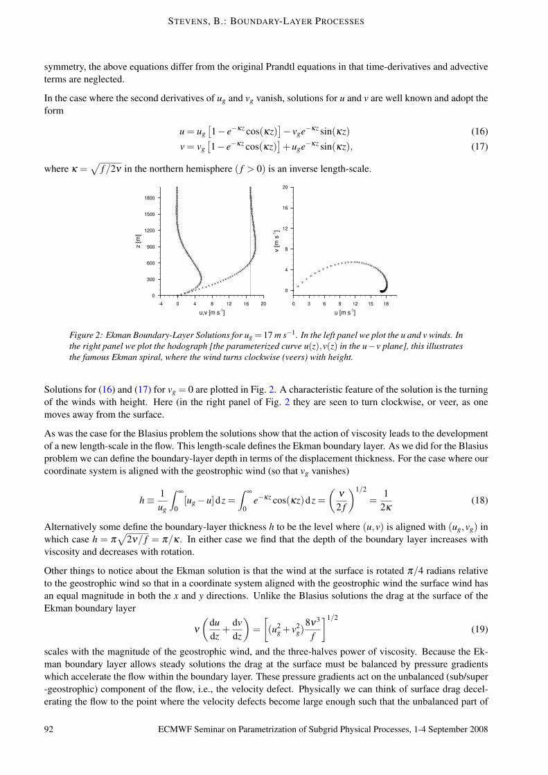
Figure 2: Ekman Boundary-Layer Solutions for ug = 17 m s−1. In the left panel we plot the u and v winds. Inthe right panel we plot the hodograph [the parameterized curve u(z),v(z) in the u−v plane], this illustratesthe famous Ekman spiral, where the wind turns clockwise (veers) with height.

Solutions for (16) and (17) for vg = 0 are plotted in Fig. 2. A characteristic feature of the solution is the turningof the winds with height. Here (in the right panel of Fig. 2 they are seen to turn clockwise, or veer, as onemoves away from the surface.

As was the case for the Blasius problem the solutions show that the action of viscosity leads to the developmentof a new length-scale in the flow. This length-scale defines the Ekman boundary layer. As we did for the Blasiusproblem we can define the boundary-layer depth in terms of the displacement thickness. For the case where ourcoordinate system is aligned with the geostrophic wind (so that vg vanishes)

h≡ 1ug

∫∞

0[ug−u]dz =

∫∞

0e−κz cos(κz)dz =

(ν

2 f

)1/2

=1

2κ(18)

Alternatively some define the boundary-layer thickness h to be the level where (u,v) is aligned with (ug,vg) inwhich case h = π

√2ν/ f = π/κ . In either case we find that the depth of the boundary layer increases with

viscosity and decreases with rotation.

Other things to notice about the Ekman solution is that the wind at the surface is rotated π/4 radians relativeto the geostrophic wind so that in a coordinate system aligned with the geostrophic wind the surface wind hasan equal magnitude in both the x and y directions. Unlike the Blasius solutions the drag at the surface of theEkman boundary layer

ν

(dudz

+dvdz

)=[(u2

g + v2g)

8ν3

f

]1/2

(19)

scales with the magnitude of the geostrophic wind, and the three-halves power of viscosity. Because the Ek-man boundary layer allows steady solutions the drag at the surface must be balanced by pressure gradientswhich accelerate the flow within the boundary layer. These pressure gradients act on the unbalanced (sub/super-geostrophic) component of the flow, i.e., the velocity defect. Physically we can think of surface drag decel-erating the flow to the point where the velocity defects become large enough such that the unbalanced part of



the pressure gradient balances the drag. As rotation weakens, the acceleration is increasingly less effective andthus must occur over an increasingly deep layer. In the limit as f → 0 h→ ∞ which is another way of sayingthat steady solutions are no longer possible.

3.3 Secondary Circulations

Both the Ekman and the Blasius boundary layers have residual vertical circulations. For the Blasius boundarylayer the convergence of the stream-wise wind drives a large-scale circulation away from the plate:

w =12

(νux

)1/2 [η f ′− f

]. (20)

In contrast the Ekman boundary layer only has an implied vertical circulation in the case when the forcingvaries spatially. By continuity, and the requirement that the undisturbed (outer) flow is divergence free,

w(z) =∫ z

0(∂xvg−∂yug)e−κz sin(κz)dz, (21)

where we note that the term in the brackets is just the geostrophic vorticity, ωg. In the case where ωg is constantwith height it can be taken outside of the integral so that

w(z) = ωg

∫ z

0e−κz sin(κz)dz = hωg. (22)

This indicates that the vertical motion is positive for cyclonic ( f ωg > 0) motion and negative for anti-cyclones.Physically we can see the effect of the boundary layer is to turn the flow in the direction of the pressuregradient. This leads to cross isobaric flow which is divergent in high pressure regions and convergent in lowpressure regions.

These residual circulations are important because they are thought to interact with the large scale flow. Forinstance in the Ekman boundary layer it is the residual circulation which organizes the tea leafs into the centerof the cup upon stirring. It is also this residual circulation which is responsible for stretching or contractingvortex tubes, thereby either spinning up or spinning down a large-scale circulation on a timescale much fasterthan the viscous timescale L/ν2. The effects of residual circulations in atmospheric analogs to Ekman flowsare precisely those effects that Charney and Eliassen recognized as critical to their representation of large-scalecirculations.

3.4 Rayleigh-Benard

The Ekman and Blasius theory form the conceptual paradigm for shear driven boundary layers. However inthe atmosphere the development of thermal boundary layers also plays a critical role. A guiding paradigm forthe thermal, or convective, boundary layer is the framework developed by Rayleigh to understand Benard’sexperiments. The experimental framework interpreted by Rayleigh is illustrated schematically in Fig. 3, andwhile it ended up being different in important respects3 from Benard’s experiments it has proven enduring. Animportant feature to note about this paradigm of convective turbulence is that the depth of the convecting layeris imposed as an independent parameter.

The non-dimensional analysis of the Bousinessq equations conforming to the sketch of Fig. 3 identifies twonon-dimensional parameters:

Ra =−g(Θ0−Θ1)h3

νκθ0and Pr =

ν

κ(23)

3In the middle part of the last century it was shown that most of the motions observed by Benard actually arose from variations inthe surface tension with temperature, not thermal instability.



r6.5cmθ0

θ1< θ0

H viscosity (ν)

cold

hot

plumes

Figure 3: Basic configuration for the Rayleigh-Benard convective instability problem.

called the Rayleigh and Prandtl numbers respectively, where now κ denotes the thermal diffusivity. Ra and Prencapsulate important aspects of convective flows. The first parameter measures how hard the system is beingdriven, the second depends on the working fluid. Given a working fluid sets the Prandtl number, leaving onlyRa free. Conceptually this is a delightful state of affairs as any two flows of a given fluid should be similar in sofar as their Rayleigh numbers are similar. Rather than having to study how convection responds to independentvariations in the temperature difference between the plates, versus variations in the depth of the convectingfluid, or the strength of the viscosity, all that is necessary is to study the behavior of the flow as a function ofthe Rayleigh number.

Insight into the Rayleigh number can be derived, for instance, by considering a parcel rising through the fluidwith the temperature, θ0 of the lower boundary. Such a parcel will accelerate through the cooler ambient fluidand will have a convective available potential energy, here measured in terms of a convective velocity scale w∗,

w2∗ =

g(Θ0−Θ1)h2Θ0

. (24)

This shows that the Rayleigh number is analogous to square of a Reynolds number defined in terms of aconvective velocity scale. It also shows that the depth of the layer, h, selects the characteristics of the flow,rather than the other way around.

The Rayleigh-Benard problem is often phrased in terms of the transition to turbulence, the character and prop-erties of the ensuing turbulent fluid and its dependence on the particulars of the boundary conditions. Othereffects, such as a mean wind, rotational effects, weakly non-linear effects and the planform structure of theconvection can all be explored (e.g., Emanuel, 1994). Scaling laws for the fully developed regime can also beinvestigated, of particular interest is the question of Ra number similarity. Apart from its analytic tractability theflow configuration also lends itself well to laboratory experiments, as such it forms a paradigm for convectivelydriven flows, such as might define the character of atmospheric boundary layers.

4 Turbulent (Planetary) Boundary Layers

A defining characteristic of the planetary boundary layer, as we have defined it, is that it is turbulent. While thelaminar boundary-layer theory helps set concepts, it is not directly applicable to the turbulent case. Turbulencearises in the atmosphere because of the range of scales and the small viscosity of the working fluid, whichnon-dimensionally is expressed in the greatness of the Reynolds, or effective Rayleigh number, of atmosphericflows.

4.1 Turbulence (Reynolds Number Similarity)

By Reynolds number similarity we typically mean that an appropriately defined Reynolds (or Rayleigh) numberis so large, that molecular effects can be neglected, i.e., , the flow behaves independently of the particular valueof its molecular properties, such as measured by the diffusivity or viscosity of the fluid. Mathematically one way



of dealing with turbulent flows is to decomposed any field of interest into an expected value and a fluctuation:

ψ = ψ +ψ′, (25)

where an over-line denotes an expected value, and ψ is an arbitrary field. At sufficiently high Reynolds orRayleigh number we expect (hope) that the divergence of the turbulent fluxes dominates that of the diffusivefluxes: ∣∣∂zu′w′

∣∣>> |ν∂zzu| , more generally∣∣∂zψ

′w′∣∣>> |ν∂zzψ| . (26)

One class of models of turbulence often assume that the fluxes are related to the structure of the flow at thesame point. The simplest of such “local” models assumes a linear relationship between local fluxes and localgradients:

ψ ′w′=−K∂zψ (27)

where the coefficient of proportionality, K has the units of diffusivity, and is often interpreted as an exchangecoefficient or an eddy diffusivity/viscosity. It may depend on the quantity being mixed, i.e., differ for scalarsversus components of the momentum. Such eddy-diffusivity models of turbulence can be rigorously justified inthe limit when the effective length-scale, `, of the mixing eddy is much smaller than the scale of variation of themean flow, a limit which generally is not well satisfied in atmospheric boundary-layer flows. The most famousexample of an eddy diffusivity model of turbulence is Prandtl’s mixing-length model, wherein turbulence isassumed to arise due to the mean shear, so that the turbulent diffusivity takes the form:

K = `2 |∂zu| .

This introduces the mixing-length `, which is assumed to be related to the scale of the turbulent eddies. Whilethis discussion focuses attention on the question of how to model the turbulent fluxes, turbulent boundary layersraise additional questions, in particular how to match the mean flow and the turbulence model to the surface, orthe flow interior. Each is an issue in the construction of models of the planetary boundary layer.

4.1.1 Turbulent momentum (shear) boundary layers

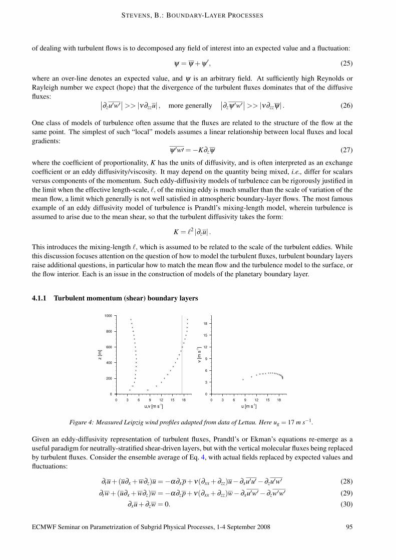
Figure 4: Measured Leipzig wind profiles adapted from data of Lettau. Here ug = 17 m s−1.

Given an eddy-diffusivity representation of turbulent fluxes, Prandtl’s or Ekman’s equations re-emerge as auseful paradigm for neutrally-stratified shear-driven layers, but with the vertical molecular fluxes being replacedby turbulent fluxes. Consider the ensemble average of Eq. 4, with actual fields replaced by expected values andfluctuations:

∂tu+(u∂x +w∂z)u =−α∂x p+ν(∂xx +∂zz)u−∂xu′u′−∂zu′w′ (28)

∂tw+(u∂x +w∂z)w =−α∂z p+ν(∂xx +∂zz)w−∂xu′w′−∂zw′w′ (29)

∂xu+∂zw = 0. (30)



So that neglecting the diffusive relative to the turbulent fluxes, and assuming the latter are horizontally homo-geneous, yields the following analog to Prandtl’s horizontal momentum equation, but now in terms of expectedvalues:

∂tu+(u∂x +w∂z)u =−α∂x p+∂z (K∂zu) , (31)

where in general K may be expected to vary with height.

Overall many of the concepts and results from laminar boundary-layer theory, in particular the Ekman solutions,can be more readily applied to the expected state of the planetary boundary layer. As an example considerthe famous Leipzig wind profiles, shown in Fig. 4, which Lettau (1950) used to derive the Eddy Diffusivity(Viscosity) profile of a nearly neutral shear layer. The main features of the Ekman solution are apparent, anddifferences principally reflect the spatial (height) variations in K. However, because K is not known a priori, butrather depends on the evolution of the flow itself, the application of such approaches to models of the planetaryboundary layer is often not as straightforward as this discussion may make it seem.

4.1.2 Turbulent thermal (convective) boundary layers

The simplest paradigm for a turbulent thermal (shear-free) boundary layer is that of a uniformly stratified fluid(such that ∂zθ = Γ) heated from below. In this case the thermodynamic equation takes the form:

∂tθ =−∂zw′θ ′ (32)

Formulating the problem in this manner (remember the pendulum) leads to a sufficiently simple state of affairsthat dimensional analysis helps pose meaningful constraints. Indeed, one can argue on dimensional grounds4,that the evolution of a thermal boundary layer should proceed such that

h = α

(QtΓ

)1/2

, (33)

where α > 1 is the non-dimensional boundary-layer depth, and Q≡ w′θ ′∣∣0 is the surface heat flux.

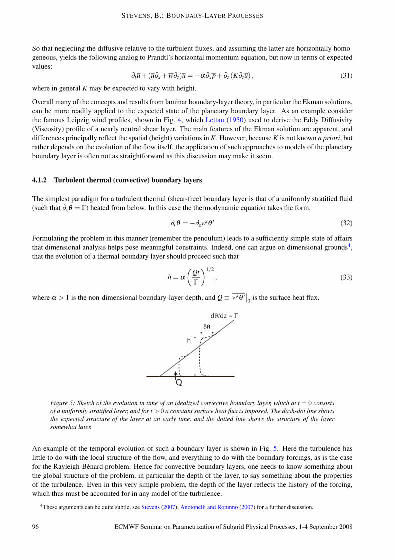
Q

dθ/dz = Γ

h

δθ

Figure 5: Sketch of the evolution in time of an idealized convective boundary layer, which at t = 0 consistsof a uniformly stratified layer, and for t > 0 a constant surface heat flux is imposed. The dash-dot line showsthe expected structure of the layer at an early time, and the dotted line shows the structure of the layersomewhat later.

An example of the temporal evolution of such a boundary layer is shown in Fig. 5. Here the turbulence haslittle to do with the local structure of the flow, and everything to do with the boundary forcings, as is the casefor the Rayleigh-Benard problem. Hence for convective boundary layers, one needs to know something aboutthe global structure of the problem, in particular the depth of the layer, to say something about the propertiesof the turbulence. Even in this very simple problem, the depth of the layer reflects the history of the forcing,which thus must be accounted for in any model of the turbulence.

4These arguments can be quite subtle, see Stevens (2007); Anotonelli and Rotunno (2007) for a further discussion.



4.2 Surface Matching

In addition to the question of how to represent the effects of turbulence on the mean flow within the boundarylayer, one must also decide how best to match the mean flow within the boundary layer to the surface below, andthe free (essentially non-turbulent and stratified) flow aloft. The question of surface matching is well addressedin the literature, but bears brief review as it helps frame some of the issues to be discussed subsequently.

The central points of the theory of surface matching again involves a combination of asymptotics and similarity.Asymptotics argues for the existence of a “surface layer” which has the characteristic of being much shallowerthan the depth of the boundary layer as a whole yet much deeper than the height of variations in surfaceproperties (e.g., what we previously denoted by z∗). In such a case, a neutrally stratified fluid can be expected todevelop velocity gradients that depend only on the velocity scale u∗ defined by the surface flux (i.e., u2

∗≡∣∣u′w′∣∣),

and the height, z above the surface, so thatz

u∗∂zu =

1k. (34)

Here k is the von Karman constant, so that 1/k is the non-dimensional velocity gradient and is presumed to beuniversal. Integrating (34) requires the additional specification of a constant, z0 (or roughness height), which isthe height at which the velocity profile would vanish if extended toward the surface (which of course it shouldnot be, as the arguments leading up to Eq. 34 presumed z� z0—hence it defines a virtual surface

When thermal effects are included an additional length-scale (measuring effectively the relative role of shearand buoyancy) emerges. This is called the Obukhov length-scale and is defined as follows:

L =− u3∗

kB. (35)

Here B is the buoyancy flux and has units of m2 s−3. The factor of k is arbitrary, but customary. L is negativein regions of positive buoyancy fluxes, i.e., where convection destabilizes the flow. Hence incorporating Bmeans that the non-dimensional velocity gradient is no longer expected to be constant, but rather to depend onthe non-dimensional height, such that

zu∗

∂zu =1k

Φ(z/L). (36)

Here Φ, the non-dimensional velocity gradient, is determined empirically (Businger, 1973). Its argument, thenon-dimensional height, z/L defines an effective Richardson number. This approach, called Monin-Obukhovsimilarity theory, can (and is) extended to describe profiles of thermodynamic properties, or passive scalars,and overall is one of the success stories in our endeavor to parameterize turbulent atmospheric processes. Itshould be familiar to most readers of this document.

Thus from the perspective of planetary boundary layers as a whole, the emergence of surface layer theorymakes two important contributions. First it introduces a length-scale, L that measures the relative contributionsof shear and buoyancy to the destabilization of the flow. Second, it means that models of the planetary boundarylayer depend only indirectly (through matching conditions) on the representation of the surface.

5 Planetary Boundary-Layer Regimes

5.1 Basic Issues

Rather simple boundary layers have been presented in terms of two classes. One in which L ≈ 0 and shear-instability is relatively unaffected by stability effects, and another wherein L� 0 and the presence of a meanflow has relatively little effect on the turbulence. For the neutrally stratified shear layers, turbulence is thoughtto exhibit a predominantly local character in that its properties reflect the local structure of the flow. Mixing-length models work well for such flows, although how best to represent the mixing-length itself remains a topic



of research. If one adopts von Karman’s initial suggestion as taking ` ∝ ∂zu/∂zzu then the logarithmic velocityprofile near the surface, as would be expected by integration of Eq. (34), implies that the distance from thelower boundary (the wall) is the only length-scale in the system, which is consistent with the assumption thatlead to (34).

On the other hand we have endeavored to argue that for convective layers, plumes convert potential to kineticenergy over the depth, h, of the convective layer. In such a situation the boundary-layer depth can be expectedto play a larger role, and the character of the turbulence depends more strongly on the structure of the layeras a whole. Moreover, how to match the vigorously-mixed convective layer, to the outer flow emerges asperhaps a more critical issue. This is evident, for instance, in a comparison of Figs. 4 and 5. For the case ofthe Leipzig wind profile the flow properties transition gradually to those of the outer layer, but for the cartoonof the convective boundary layer there is a distinct transition layer (the so-called entrainment interfacial layer)separating the convective layer from the outer layer.

What about L� 0? In this case we expect shear and stability effects to work against one another, as buoyancyeffects will resist the tendency of shear-flow instability to destabilize the flow. Such stability effects can bemeasured by the Brunt-Vaisalla frequency, N2 = g

Θ∂zθ thereby introducing another timescale into the flow.

So for instance, for stable Ekman layers one could look for solutions as a function of N/ f . The effect ofstability introduces further complications as it supports waves and intermittency (bursts, perhaps associatedwith breaking waves) in the turbulent activity, which greatly complicates the treatment of such layers.

In summary, even for very basic planetary boundary layers the dimensionality of the solution space is non-trivial. In addition to L which characterizes the surface driving, the boundary-layer depth, h, the Coriolisparameter f , and (at least for stably stratified layers) N2, all emerge as parameters. Among these, both h and Lare ambiguous as they depend on the character of the flow itself. But if one can take them as given it says thatthe structure of the planetary boundary layer, in even the simplest circumstances, should depend on at least twonon-dimensional numbers, h/L and f /N.

5.2 Complications

Of course nature is much more complex than this. Indeed, one might argue that the planetary boundary layeris best defined by the complexity of the regimes it encompasses. In this section we just try to develop a tastefor some of the complicating factors, and their relevancy to outstanding issues in our endeavor to represent theeffects of boundary-layer processes in weather and climate.

5.3 Baroclinicity

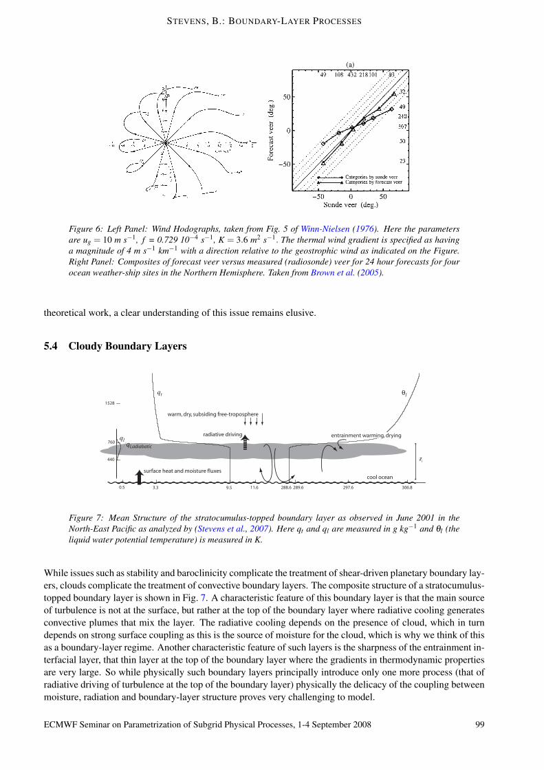
One important complication, is also an original one, as it was a focus of the introductory remarks of Winn-Nielsen (1976). And that is the effect of baroclinicity, i.e., vertical shear in the geostrophic wind arising fromlarge-horizontal temperature gradients. Even such a simple change to the experimental configuration (Ekman’sproblem) effectively introduces two additional timescales into the problem. Winn-Nielsen (1976) among othersshowed that these baroclinic effects can significantly alter the character of the Ekman spiral, and that for someconditions the winds can be expected to back (turn counter-clockwise) rather than veer with height. An exampleis shown in the left panel of Fig.6. These different wind profiles in turn are characterized by distinctly differentsecondary circulations, with concomitant effects on the mean flow.

The difficulty state-of-the-art boundary-layer representations have in capturing such effects, is illustrated in arecent study by Brown et al. (2005) from which the right panel in Fig. 6 is excerpted. The figure shows thatthe wind turning in the boundary layer is less pronounced in the model than it is in the data. Brown showsthat reducing the mixing in stable boundary layers tends to mitigate this issue, but exacerbate other problems,particularly over land where enhanced mixing of momentum in situations where one would not expect muchturbulent exchange improves the forecast skill of the model (see Beljaars, 1994). Notwithstanding the extensive



Figure 6: Left Panel: Wind Hodographs, taken from Fig. 5 of Winn-Nielsen (1976). Here the parametersare ug = 10 m s−1, f = 0.729 10−4 s−1, K = 3.6 m2 s−1. The thermal wind gradient is specified as havinga magnitude of 4 m s−1 km−1 with a direction relative to the geostrophic wind as indicated on the Figure.Right Panel: Composites of forecast veer versus measured (radiosonde) veer for 24 hour forecasts for fourocean weather-ship sites in the Northern Hemisphere. Taken from Brown et al. (2005).

theoretical work, a clear understanding of this issue remains elusive.

5.4 Cloudy Boundary Layers

surface heat and moisture fluxes

radiative driving

cool ocean

qt θl

warm, dry, subsiding free-troposphere

zi

ql ql,adiabatic

0.5 3.3 9.5 11.6 288.6 297.6 306.8

entrainment warming, drying

1528

760

440

289.6

Figure 7: Mean Structure of the stratocumulus-topped boundary layer as observed in June 2001 in theNorth-East Pacific as analyzed by (Stevens et al., 2007). Here qt and ql are measured in g kg−1 and θl (theliquid water potential temperature) is measured in K.

While issues such as stability and baroclinicity complicate the treatment of shear-driven planetary boundary lay-ers, clouds complicate the treatment of convective boundary layers. The composite structure of a stratocumulus-topped boundary layer is shown in Fig. 7. A characteristic feature of this boundary layer is that the main sourceof turbulence is not at the surface, but rather at the top of the boundary layer where radiative cooling generatesconvective plumes that mix the layer. The radiative cooling depends on the presence of cloud, which in turndepends on strong surface coupling as this is the source of moisture for the cloud, which is why we think of thisas a boundary-layer regime. Another characteristic feature of such layers is the sharpness of the entrainment in-terfacial layer, that thin layer at the top of the boundary layer where the gradients in thermodynamic propertiesare very large. So while physically such boundary layers principally introduce only one more process (that ofradiative driving of turbulence at the top of the boundary layer) physically the delicacy of the coupling betweenmoisture, radiation and boundary-layer structure proves very challenging to model.



10ql

ERA-40

IFS

GFS

q [gkg-1] θ [K]

z [m]

Figure 8: Mean Structure of the stratocumulus-topped boundary layer as represented in the ERA40, theIFS and the GFS for the period and time corresponding to the observations presented in Fig. 7, taken from(Stevens et al., 2007).

This point is illustrated in Fig. 8 where the model representation of the boundary layer observed in Fig. 7is presented. Here we see that the models “resolve” the transition between the boundary layer and the free-troposphere over the characteristic 5-6 grid points. Because the vertical discretization is so coarse, this resultsin a much diffuser transition which distorts the mixing processes between the troposphere and the boundarylayer, and hence the properties of the boundary-layer state (see for instance the thermal structure of the globalforecast system (GFS) model). As a result the amount of cloud in the modeled boundary layer tends to be toolittle (here underestimated by at least a factor of ten), which results in insufficient radiative cooling to driveturbulence and mixing within the boundary layer.

5.5 And So On

The complications, of course, do not end here. As our demands of global models increase, myriad otherquestions come into play. A by no means non-exhaustive list includes: the coupling of the planetary boundarylayer to clouds that evacuate mass from the boundary layer (for instance the cumulus topped boundary layersdiscussed by Siebesma, 1998), but also the coupling of boundary layers to canopies, water waves, complexunderlying orography and so on.

6 Discussion & Outlook

In this presentation I have endeavored to develop the big picture of boundary-layer processes, and the recurringthemes that emerge from such a picture. The first is that the boundary layer indeed embodies the concept of adistinct (sometimes very distinct) layer of the atmosphere, one in which vertical transport (through turbulence)and surface coupling are very active. The depth of this layer plays an important role in the character of theturbulence, particularly for convective layers. The driving forces of turbulence are either shear in the horizontalwinds, or convection. Shear is usually manifest through the drag at the surface, but also modified by stabilityand varying pressure gradients (for instance in baroclinic boundary layers). Convection emerges from surfaceheating, for conventional boundary layers over land, but also can arise due to radiative processes acting at thetop of the boundary layer (such as one finds in stratocumulus layer).

Approaches to modeling boundary layers are varied; but invariably are faced with similar questions. What is theboundary-layer depth? What type of mixing rule is required within the boundary layer? How is the boundarylayer coupled to the free-troposphere above, versus the surface below? Depending on one’s emphasis, verydifferent types of models emerge to address these questions. Interest in convective layers favors the use of



global rules, in that the mixing depends on the structure of the layer as a whole; while interest in shear andmomentum boundary layers favor local approaches. More fundamentally, models differ in whether one viewsboundary layers in terms of idealized regimes (through which similarity approaches might be useful to lendinsight into their workings) or the outcome of specific processes.

In the former approach (regime based methods) models are first tasked with identifying the regime and thenapplying appropriate mixing rules. In the latter processes are allowed to compete in the hope that they will findthe correct regime. An example of a regime based model is that of the UK Met Office (Lock, 2004). Regimebased methods suffer from the need to identify a small set or regimes (to be practical) and the question of howto deal with intermediate regimes. Process based methods have the potential of being more general, but dependon a mature understanding and capacity for modeling the underlying processes, and resolving their verticalstructure—something which most large-scale models still fail to do.

Throughout most of this discussion we have identified boundary layers as ideas, abstractions. This may besomewhat old fashioned. Increasingly interest is demanding representations of planetary boundary layers thatbreak the classifications we wish, for reasons of theory and tractability, to confine them too. For instance asmodels represent ever more processes at ever finer resolution, interest in layers where h may be smaller than Lis encouraged, as is interest in layers where turbulence is not continually coupling the flow to the surface, or inrepresentations where statistical theories become less applicable. In all challenges continue to mount; but thenso do the opportunities for new and novel contributions.

Acknowledgments

The author would like to thank the organizers of this seminar, and in particular Anton Beljaars for many helpfuldiscussions.

References

Anotonelli, M. and R. Rotunno, 2007: Large-eddy simulation of the onset of the sea breeze. J. Atmos. Sci., 64,4445–4457.

Arya, P. and J. Holton, 2001: Introduction to Micrometeorology. Academic Press.

Atkins, N. T., R. M. Wakimoto, and C. L. Ziegler, 1998: Observations of the finescale structure of a drylineduring VORTEX 95. Mon. Wea. Rev., 126, 525–550.

Barenblatt, G., 1996: Scaling, self-similarity, and intermediate asymptotics. Cambgridge, Cambridge, NewYork, Melbourne.

Beljaars, A., 1994: The impact of some aspects of the planetary boundary layer scheme in the ECMWF model.Seminar on Parametrization of Sub-grid Scale Physical Processes, 5-9 September 1994, ECMWF, ShinfieldPark, Reading, United Kingdom, 125–162.

Brown, A., A. Beljaars, H. Hersbach, A. Hollingswroth, M.Miller, and D.Vasiljevic, 2005: Wind turning acrossthe marine atmospheric boundary layer. Quart. J. Roy. Meteor. Soc., 131, 1233–1250.

Businger, J., 1973: Workshop on Micrometeorology, American Meteorological Society, Boston, MA, chapterTurbulent transfer in the atmospheric surface layer. 67–100.

Charney, J. G. and A. Eliassen, 1964: On the growth of the hurricane depression. J. Atmos. Sci., 21, 68–75.

Emanuel, K. A., 1994: Atmospheric Convection. Oxford, New York, Oxford, pp. 580.



Garratt, J. R., 1992: The atmospheric boundary layer. Cambridge, 372 pp.

Holtslag, A. and P.G.Duynkerke, eds., 1998: Clear and Cloud Boundary Layers, volume 48. Royal NetherlandsAcademy of Arts and Sciences.

Khairoutdinov, M. and D. A. Randall, 2006: High-resolution simulation of shallow-to-deep convection transi-tion over land. J. Atmos. Sci., 63, 3421–3436.

Lettau, H., 1950: A re-examination of the ”Leipzig Wind Profile” considering some relations between windand turbulence in the frictional layer. Tellus, 2, 125–129.

Lock, A., 2004: The sensitivity of a gcm’s marine stratocumulus to cloud-top entrainment. Quart. J. Roy.Meteor. Soc., 130, 3323–3338.

Moskowitz, B. M. and C. S. Bretherton, 2000: An analysis of frictional feedback on a moist equatorial kelvinmode. J. Atmos. Sci., 57, 2188–2206.

Ooyama, K., 1964: A dynamical model for the study of tropical cyclone development. Geophys. Int.,, 4, 187–198.

Schlichting, H., 1979: Boundary Layer Theory. McGraw Hill, New York, 7th edition.

Siebesma, A. P., 1998: Shallow convection. Buoyant convection in Geophysical Flows, E. J. Plate, E. E. Fe-dorovich, D. X. Viegas, and J. C. Wyngaard, eds., Kluwer Academic Publishers, Dordrecht, The Netherlands,volume 513 of C, 441–486.

Stevens, B., 2007: On the growth of layers of non-precipitating cumulus convection. J. Atmos. Sci., 64, 2916–2931, in press.

Stevens, B., A. Beljaars, S. Bordoni, C. Holloway, M. Kohler, S. K. V. Savic-Jovcic, and Y. Zhang, 2007: Onthe sturcture of the lower troposphere in the summertime stratocumulus regime of the northeast Pacific. Mon.Wea. Rev., 135, 985–1004.

Winn-Nielsen, A., 1976: Introductory remarks. Seminar on the Treatment of the Boundary Layer in NumericalWeather Prediction, 6-10 September 1976, ECMWF, Shinfield Park, Reading, United Kingdom, 1–15.

Wippermann, F., 1976: Theoretical aspects of the planetary boundar layer. Seminar on the Treatment of theBoundary Layer in Numerical Weather Prediction, 6-10 September 1976, ECMWF, Shinfield Park, Reading,United Kingdom, 39–76.


boundary-layer processes for weather and climate

Documents