boundary layers and homogenlzatlon of transport...
TRANSCRIPT

Publ. RIMS, Kyoto Univ.15 (1979), 53-157
Boundary Layers and Homogenlzatlonof Transport Processes
By
Alain BENSOUSSAN*. Jacques L. LlONS*
and George C. PAPANICOLAOU**1}
Contents
Page§0. Introduction. 54
§1. Physical theory of transport processes.
1. 1. The transport equation. 55
1. 2. Boundary conditions. 57
1. 3. Existence and uniqueness. 60
1. 4. Cellular geometry, homogenization and force fields. 64
1. 5. Half-space problems. 66
§2. Probabilistic theory of transport processes.
2. 1. Construction of transport processes. 71
2. 2. Boundary conditions. 75
2. 3. Connection with the physical theory. 83
2. 4. Asymptotic problems and homogenization. 87
2. 5. Ergodic properties of transport operators. 89
2. 6. Reflection and transmission operators for
half-space problems. 96
2. 7. Potential theory for the half-space problem. 106
§3. Diffusion approximations.
3. 1. Asymptotic expansion in an unbounded region
and homogenization. 115
Communicated by K. Ito, July 7, 1976. Revised August 15, 1977.* I. R. L A., Laboria, Laboratoire de Recherche en Informatique et Automatique,
Domaine de Voluceau-Rocquencourt, 78150 Le Chesnay, France.** Courant Institute of Mathematical Sciences, New York University, 251 Mercer Street,
New York, N. Y. 10012, U. S. A.15 Supported by an Alfred P. Sloan Foundation Fellowship and by the Air Force Office
of Scientific Research under Grant No. AFOSR-76-2884.

54 ALAIN BENSOUSSAN, JACQUES L. LIONS AND GEORGE C. PAPANICOLAOU
3. 2. Validity of the expansion. 121
3. 3. Weak convergence of the process. 122
3. 4. Boundary layer coordinates. 129
3. 5. Asymptotic expansions for absorbing boundary
conditions (without cells). 132
3. 6. Asymptotic expansion for reflecting boundary
conditions (without cells). 138
3. 7. Weak convergence of reflected process. 146
References 156
§ 00 Introduction
This work started as a continuation of [1] but in the meantime the
scope of the project widened and the intimate connection -with homogeniza-
tion problems [2, 3] became apparent. The contents are briefly as follows.
In Section 1 we review for completeness the physics of transport
processes. We focus on those points that bear upon the asymptotic analy-
sis when the mean free path tends to zero. We refer to [1] for many
references to related work and to [4, 5] for additional information on
asymptotic problems.
In Section 2 we give a probabilistic description of linear transport
processes much like in [1]. The material is standard in the theory of
Markov processes. The theorem at the end of Section 2. 5 and the results
of Sections 2. 6 and 2. 7 are of direct interest to the asymptotics. They
are also of independent interest.
Section 3 contains the main results, namely the asymptotic limit of
small mean free path in transport theory. Without cellular-space struc-
ture (i.e., without homogenization) the results are fairly complete al-
though interface problems are not treated. With cellular structure and
boundary layers the analysis has yet to be carried out. We employ the
theory of Stroock and Varadhan [6] which seems to be just the right
tool for our problems.
The analysis herein is restricted to transport problems that involve
scattering only (no fission) to highest order in the mean free path param-
eter. Processes that involve particle creation, multiplicative processes, can

BOUNDARY LAYERS OF TRANSPORT PROCESSES 55
be formulated as branching transport processes. Their asymptotic analysis
requires several additional considerations not given here (cf. [21]).
The general scheme by which asymptotic results are obtained is to
first construct formal asymptotic expansions in the usual way as in [4, 5,
8] and in Sections 3. 1, 3. 5 and 3. 6. Sections 2. 5, 2. 6 and 2. 7 provide
simple sufficient conditions for the existence of such expansions. Then
we prove that the expansions are truly asymptotic. To prove limit theo-
rems (invariance principles) we follow along the lines of [6] and the
set-up abstracted by Kurtz in [7]; this is done in 3. 3 and 3. 7.
We thank M. Williams and E. Larsen for many discussions on the
problems considered here. We also thank the referee of the paper for
carefully reading the manuscript and suggesting many improvements and
corrections.
Finally we thank S. R. S. Varadhan for generously sharing with us
his insight into the problems considered here and introducing us to many
important ideas and techniques which enter into much of what follows.
§ 1. Physical Theory of Transport Processes
1.1. The Transport Equation
In many physical phenomena the quantities of interest satisfy, within
certain reasonable approximations, linear transport equations. Radiative
transport theory [9, 10] and neutron transport theory [11,12,13] are
perhaps the best known examples of physical theories leading to the
transport equation we shall study here. Gas dynamics on the other hand
leads to Boltzmann's equation [14, 15, 16] which is nonlinear. The re-
levant linearizations of this equation do not admit the kind of probabilistic
treatment we intend to give so we shall not discuss gas dynamics here.
Let (j)(t,x7 v) denote the density of particles at time £>0, at location
x<EiIC and with velocity v^Rs. The word "particles" stands for photons
or neutrons depending on the context and will be used throughout in a
generic sense. The particles move on straight lines in the absence of
collisions. We assume that they collide with obstacles in the underlying
medium and that the latter are not affected by the collisions; the particles

56 ALAIN BENSOUSSAN, JACQUES L. LIONS AND GEORGE C. PAPANICOLAOU
do not collide with each other. The last assumption leads to a linear
conservation equation for <f) which we now describe.
In the interval (t, t + Jt) we have
9 9 A p
dt dx
This is the total derivative of <p and v- - stands for the dot productdx
of v and the x gradient. In the same time interval 0 (t, x, v) increases
as a result of collisions at x, t which convert particles of velocity v'=£v
into particles of velocity v. It decreases as a result of collisions that
convert particles of velocity v to velocities v'^v. Let 2(t* x, v, v') de-
note the fraction of particles per unit time converted from velocity v' to
velocity v and assume it is a continuous function of v and T/. Let
6 (t, x, v) denote the fraction of particles per unit time converted to veloc-
ity vf=f=^v. Then we have
, v) - t f > ( t , x , v)
where the integral is over all velocities in Rs. Combining the above
expressions we get the transport equation
Q 1 1) 9 ( t > ( t 9 x 9 v ) Q<t>(t9x9v)dt dx
The functions 2 and 6 are called the differential and the total scattering
cross-section respectively.
Equation (1. 1. 1) must be supplemented with initial and boundary
conditions. In the absence of boundaries, xEiR3 and (1.1.1) is to hold
in all of jR3 for both x and v and
(1.1.2) tf(0,;r,tO=00(a:,tO
a given initial particle density. Boundary conditions are considered in the
next section.

BOUNDARY LAYERS OF TRANSPORT PROCESSES 57
If for each x and t we have
(1. 1. 3) f-T (*, .r, v', v) dvf = ff (t, .r, v) ,
then the collisions are called pointwise conservative; there is no creation
or anihilation of particles. As a consequence I I (f)dvdx, the total num-
ber of particles, does not change in time. If the left hand side of (1. 1. 3)
exceeds the right hand side then we have net creation of particles; other-
wise net destruction. In many important problems (1. 1. 3) does not hold
pointwise but the solutions of (1. 1. 1) admit nontrivial steady-state be-
havior. Such situations are also called conservative but they are clearly
different from (1. 1. 3) . To emphasize the difference we shall refer to
(1. 1. 3) as the pointwise conservative case.
I. 2 Boundary Conditions
Let £D be a domain in R*. A typical boundary value problem is the
following
(1.2.1) JM_ + t;.JM-=,dt dx
Here n denotes the unit outer normal to the boundary dS) of 3), Pro-
blem (1. 2. 1) is well defined as can be seen from the following conside-
rations. Let dS denote a surface element at x with normal n. Then
n -v<f>(t, x, v) dSdvdt is the number of particles crossing dS at x with
velocity v within, dv and at time t within dt. To confirm this we inte-
grate (1. 2. 1) and use Green's Theorem to obtain the identity
(1.2.2) ( \<l>(t,x,v)dvdx+ \ \ \ ti>v(!)(s,x,v}J® J JO JdS) Jn.tf>0
= I I 0o (xy v} dxdv +1 I \ffs (5, .r, v) (f) (t, x9 v) dvdxdsJff> J Jo J<fl J
-h 1 I Q(s9 x, v} dvdSds .Jo JdiD Jn>v<V

58 ALAIN BENSOUSSAN, JACQUES L. LIONS AND GEORGE C. PAPANICOLAOU
The left hand side of (1. 2. 2) represents the total number of particles in
S) at time t plus the total number of particles that exited from 3) up to
time t. The right hand side is the total number of particles present at
time t = Q plus the total number that entered 3) through the boundary
up to time t and (the middle term) the total number that were created
in S) up to time t. We have defined ff, by
(1. 2. 3) (T, (t, x, v) = {l (t, x, v', v) dvf - ff (t, x, v) .
Uniqueness for (1. 2. 1) is easily established from (1. 2. 2) , assuming that
, because 0>0 and we have the inequality
< \ W0(x,v)dxdv + iff g(s,x,v)dvdSds + M I ®(s)ds ,JS) J JO Jd$ Jn.<<0 JO
where
(0 (*) = f \(f) (t, x, v} dvdx .
Existence is discussed in the next section and again in Section 2. 1 in a
probabilistic setting.
Another typical boundary value problem involves reflection of parti-
cles at the boundary. Let B(t,x,v,vf} denote the fraction of particles
which at the point x^dS) and at time t are converted from outgoing
with velocity v' (n-vf^>Q>) to incoming with velocity v (n-v<^Q). The
reflecting boundary value problem is then
(1.2.4) .+ v--= s<l>dv'-(I<l>, x<=£), v(=R3, t>Q 9dt dx
(1.2.5) - f t -
= f B(t, x, v, v'} n-v'<j>(t,x,v'}dv' + g (t, x, v} ,Jn.«'>0
The left hand side of (1. 2. 5) is the flux of particles incoming at the
boundary and the right hand side is the incoming flux due to reflection
plus the incoming flux due to exterior sources.

BOUNDARY LAYERS OF TRANSPORT PROCESSES 59
Let us denote by ffB(t,x,v), n-v^Q, the fraction of particles reflec-
ted at x^d£), £>0, which arrived at the boundary with velocity v.
Then,
(1.2.6) ffB(t,x,v)= ( B(t,x9v',v)dv'Jn.t>'<0
and hence, from (1. 2. 5)
(1.2.7) - f n-v<j)(t,x,v}dvJw.»<0
= G B ( t 9 J C , v ) n - v < f > ( t , j ; , v ) d v + cj (t, x, v) dv ,Jn«tJ>0 Jn-t?<0
Equation (1. 2. 7) is the analog of (1. 2. 2) at the boundary points, i.e.,
it is the law of conservation of flux at the boundary.
When ffB(t,x,v)=l then we have total reflection at the boundary.
In general, 0<<T5(£, x, v) <1 and strict inequality on the right corresponds
to partial reflection at the boundary.
At the interface between two adjoining media boundary conditions are
imposed to preserve continuity of flux. Thus, if 0: (t, x, v) and 02 (t, x, v)
denote the particle density in S)l and S)2 respectively, we have the follow-
ing boundary value problem (assume no reflection) .
(1.2.8) + ^ . ^ ^Jt/-^, x^S)^ vtERs, O>0,dt dx
(1.2.9) - + v.<=dt dx
0! (0, x, v} = 0oi (*, v)
(j)2 (0, X, V) = 002 (X, V)
(1. 2. 10) - n, - vfa (t, x, v) = g1 (t, x, v) ,
— nz ' v(j)z (f, x, v) = g2 (t, x, v) 5
.re 95),,
(1. 2.11) - Hi - vfa (t, x, v) = nz • vfa (t, x, v) ,

60 ALAIN BENSOUSSAN, JACQUES L. LIONS AND GEORGE C. PAPANICOLAOU
nz • vfa (t, x, v)=Hl- vfa (t, x, v) ,
Clearly (1.2.11) can be written simply as (since n1=—n2
(1.2.110 <t>i(t,x,v)=fa(t,x9v)9
However, it is appropriate to write (1. 2. 11) since this is the general
statement of flux continuity. If the motion inside 3)l and S)z is not
linear between collisions (see the probabilistic treatment) , then the multi-
plicative factors in (1. 2. 11) need not cancel in general.
I, 3, Existence and Uniqueness
The existence of solutions to (1. 2. 1) which we shall outline yields
also that 0 is nonnegative if the data is nonnegative. Therefore, the
conservation law (1. 2. 2) yields uniqueness if \ffg <^M<^oo. In the par-
tially reflecting case instead of (1. 2. 2) we have the conservation equation
(1.3.1) f {<f>(t,x,v)dvdx + f f f fi'V^(s9x9v^J<2> J -JO J9<2) Jn.w>0
= I 0o (x9 v} dxdv 4-1 j I ff, (s9 x, v) (f) (s9 x, v) dvdxds
I 1 I 6B(s9x9v)ii' v(j) (5, x, v) dvdSdsJO JdS) Jn-u>0
I I I 0 ( 5 > x » w ) dvdSds .Jo JdS) Jn.u>0
+
Here we have used (1.2.6). From (1.3.1) and the fact that 0<(T5<1
uniqueness follows as for (1. 2. 1) .
We pass now to the question of existence and we shall restrict atten-
tion to (1. 2. 1) with 3) a bounded open set in JR3. One must distinguish
two cases here. When the differential scattering cross-section 2(t, x, v, v')
is a symmetric function of v and v' the existence theory for (1. 2. 1)
is identical to the one for its adjoint and thus it will follow from the
general considerations of Sections 2.1, 2. 2. Problem (1. 2. 1) is well-
posed under very general conditions on the data and for £e [0, T],

BOUNDARY LAYERS OF TRANSPORT PROCESSES 61
but arbitrary.
When 2 is not symmetric the existence theory for (1. 2. 1) follows
in a weak sense from the probabilistic treatment. The iteration argument
below leads directly to the desired results as we now show.
First we rewrite (1. 2. 1) as an integral equation by the usual method
of characteristics. Let t = ts)(x,v) denote the time for a particle to reach
starting from x^S) and moving with velocity — v. Then we have
(1. 3. 2) 0 (*, x,v)=i (/</*) 0o Or - vt, r;)
/ rtX exp — I 6(s.x — v(t — s), v) d
\ Jo
Q 0 — ts>,x — vt^ v)n -v
X exp — 1 (7 (s, x — v (t — s) , v) ds}-® I
Ct
~ $(r,x~v(t-r},v)JS
X £(s,x- v(l—s), v, v')<j>(js,x — v(t — s)9 v')dv'ds .
,A, expt/\tg
Here t f\tg = m.m(l,, f&) and ^(^<f^) equals one if t<^l^ and zero other-
wise. We assume that the data 00 and g are compatible, i.e. for x^dS),
n-v<Q, 00 (x, v) = g (0, x, v) . We also assume that — (TZ -77) -1g (t, x, v)
is uniformly bounded x<^d3), n-v<0 and 0<^<T<oo.
Regarding the ^/-behavior of the data 00>0 and g>0, and the scat-
tering cross-section 2 we assume the following
(1. 3. 3) [sup oCr, T;) dv<oo ,J e.^
(1.3.4) I sup sup g(^? :, v)dv<^oo ,J t>0 J-E95)
(1. 3. 5) I sup sup sup 2 (t, x, v'9 v)dv' <^oo .** t^ X<=® WGJJ3
These hypotheses are quite reasonable especially when there is a cut-off
in velocity space so only velocities of up to a finite magnitude enter into
the problem. Regarding the total scattering cross-section (J we assume
that

62 ALAIN BENSOUSSAN, JACQUES L. LIONS AND GEORGE C. PAPANICOLAOU
(1. 3. 6) 0<(T<M<oo .
Now (1. 3. 2) can be solved by iteration. We let
(I. 3.7) 0(0) (*,•£, v}
t r\ Jo '
ift (f /• /y. irtf cvj\y \*' "S)) •*- Vl'fQj UJ
n -v
/ pX 6Xp I — I 0 \S' X — "V (t — S) 9 *Uj t
\ Jt-tcD
and
where
(1. 3. 9) KJ (t, x, v} = |£_tA^exp ( - p (r, x-v(t-rt,v)
r ^ ' fj > jFrom these definitions we find that
I sup sup 0(0) (t9 x9 v) dv<C<^oo
and inductively
I sup 0(7I) (2, x. v)dv<- —CJ x^ ~ n!
where C and C' are constants in view of our assumptions8 Since the
solution 0 of (1. 3. 2) is formally
our estimates above show that this series converges and $ exists in the
norm
(1. 3. 10) J sup sup |00, .r, v) \dvJ Q^s^t x^Q
This concludes the proof of existence.
BOUNDARY LAYERS OF TRANSPORT PROCESSES 63
The bounds obtained above for the iteration process are, of course,
very crude and behave very poorly for t large. On the other hand the
large t behavior of solutions to (1. 3. 2) is a much more difficult problem;
it is actually an eigenvalue problem. Uniqueness, as observed earlier,
follows simply from conservation relations such as (1. 2. 2) or also, from
(1.3.2).
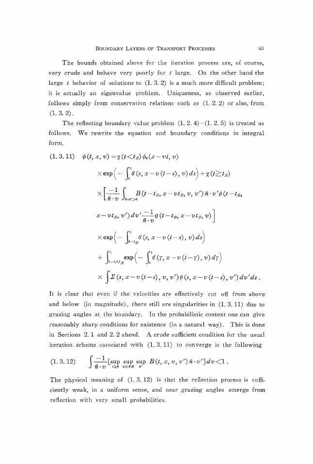
The reflecting boundary value problem (1. 2. 4) - (1. 2. 5) is treated as
follows. We rewrite the equation and boundary conditions in integral
form.
(1. 3. 11) 0 (*, x, v) = K (*<**) 0o (x - vt, v)
/ nXexp - G(s,x-v(t-s)9
\ Jo
X -1— E(t~t^xLfi -V Jn.t>'>0
x — vt®, v')dv' - <7 (£ — £<£, •£ — vt®, v)n-v J
/ r \X exp ( — I ff (s x — v (t — s) , v) ds\-
exp
\2(s9x-v(t — s)9 v, v')(j>(s,x-v(t-s), v')dv'ds .
It is clear that even if the velocities are effectively cut off from above
and below (in magnitude) , there still are singularities in (1. 3. 11) due to
grazing angles at the boundary. In the probabilistic context one can give
reasonably sharp conditions for existence (in a natural way) . This is done
in Sections 2. 1 and 2. 2 ahead. A crude sufficient condition for the usual
iteration scheme associated with (1. 3. 11) to converge is the following
(1.3.12) [-^-[sup sup sup B(t,x, v, v'} n « v'~\dv <\ .J n " v ^° x^ds) v
The physical meaning of (1. 3. 12) is that the reflection process is suffi-
ciently weak, in a uniform sense, and near grazing angles emerge from
reflection with very small probabilities.
64 ALAIN BENSOUSSAN, JACQUES L. LIONS AND GEORGE C. PAPANICOLAOU
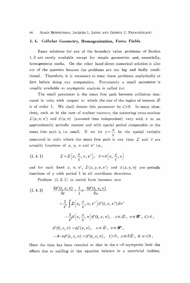
I. 4. Cellular Geometry, Homogenizatioii, Force Fields
Exact solutions for any of the boundary value problems of Section
1. 2 are rarely available except for simple geometries and, essentially,
homogeneous media. On the other hand direct numerical solution is also
out of the question because the problems are too big and badly condi-
tioned. Therefore, it is necessary to treat these problems analytically at
first before doing any computation. Fortunately a small parameter is
usually available so asymptotic analysis is called for.
The small parameter is the mean free path between collisions mea-
sured in units with respect to which the size of the region of interest S)
is of order 1. We shall denote this parameter by £>0. In many situa-
tions, such as in the case of nuclear reactors, the scattering cross-sections
S(x9v9v') and G(x9v) (assumed time independent) vary with x in an
approximately periodic manner and with spatial period comparable to the
mean free path e, i.e. small. If we let y = — be the spatial variable
measured in units where the mean free path is one then H and G are
actually functions of x9 y, v and vf i.e.,
(1. 4. 1)
and for each fixed x, v, v', 2(x9y9v9v') and G(x9y9v) are periodic
functions of y with period 1 in all coordinate directions.
Problem (1. 2. 1) in scaled form becomes now
(1,4.2)dt s dx
v v < t x
J- x-/ "t- _. \ JB f J. _. _ A _ . .— sr\ _. — TIS /^\.nZ i ' - / - ' - - ? ^ *
-n-v<jf(t,x,v)=ge(t,x,v), O>0,
Here the time has been rescaled so that in the £^>0 asymptotic limit the
effects due to scalling in the equation balance in a nontrivial fashion.

BOUNDARY LAYERS OF TRANSPORT PROCESSES 65
The data ,$0e and gs depend on £ in general. The basic problem is to
study the behavior of 0e as e—»0 and obtain asymptotic expansions.
The geometry of the above problem, where the coefficients vary rapid-
ly in a periodic manner, is referred to as the cellular geometry. The
limit we seek to analyze is the homogenization limit, so called because
the first approximation usually satisfies an equation with spatially aver-
aged, i.e. homogenized, coefficients. In addition, a small mean free path
limit or a diffusion limit is superimposed in (1. 4. 2). A description of
the above problem can be found in [5].
The results of Section 3 show that the solution $* of (1. 4. 2) can be
constructed by solving homogenized diffusion equations and half-space pro-
blems^ The probabilisitc formulation assists in finding natural hypotheses
for the validity of the expansions and yields more insight into the struc-
ture of the limits.
The reflecting boundary value problem (1. 2. 4), (1. 2. 5) is scaled
the same way. The boundary reflection function B will in general depend
on e now, and, it will turn out later, the principal term of B must be
totally reflecting, i.e. (TB=1 in (1. 2. 6).
The interface problem (1. 2. 8) - (1. 2. 11) with the scaling of (1. 4. 2)
remains, intact and it is, in fact, a very important problem in nuclear
engineering where the two media S)l and £D2 are the core and the
moderator (or reflector) respectively. The core is a problem with rapid
periodic spatial variations while in the moderator only a diffusion ap-
proximation is sought.
Force fields can also exist. In general linear transport theory most
problems of interest lead to equations which have abstractly the form
(i.4.3) M^j^i^'H-j^', 0»(0) =0,,(Jt- o £
where Jd, £% and jCs are linear operators. The asymptotic analysis of
Section 3 applies formally to any such problem provided some general
conditions are supposed to hold. It is more difficult however to find
simple sufficient conditions for the validity of the formal expansions.
In Section 3 we do not consider cellular structure and boundary layers simultaneously.

66 ALAIN BENSOUSSAN, JACQUES L. LIONS AND GEORGE C. PAPANICOLAOU
1. 5* Half-Space Problems
Half-space problems are perhaps the only nontrivial boundary value
problems that admit reasonably explicit analytical solutions. They have
been studied extensively [9, 11] by essentially two different methods. The
first is invariant imbedding [9] which lends itself readily to numerical
analysis. The second is by eigenfunction expansion [11] where a careful
analysis is needed to obtain the necessary orthogonality relations.
From the viewpoint of asymptotic analysis centered about the diffusion
approximation, half-space problems enter in the boundary layer analysis.
Here the diffusion solution is matched to that of an appropriately local-
ized half-space problem. However, a relatively small portion of the full
solution of the half-space problem enters the asymptotic formulas and this
is an additional simplifying feature.
We consider the half-space problem in connection with the diffusion
approximation without homogenization. It is time-homogeneous and under
the additional hypothesis that the velocities take values on the unit sphere
we have that $ = $(&, jtt) , x<Q9 — 1<C/£<;1, C# = ^-component of veloc-
ity) satisfying
(1.5.1)
Perturbation theory requires, in addition, that
a. 5. 2)i.e. the half-space problem is conservative. If (1. 5. 2) is not satisfied,
the asymptotic expansions have a degenerate form which is less interesting
(and actually simpler to analyze) than when (1. 5. 2) holds.
We require the following qualitative properties from (1. 5. 1) under
(1. 5. 2) :
(i) The limit \\mx_,_x (fr^x* /JL) exists for each
(1.5.3)
and is independent of

BOUNDARY LAYERS OF TRANSPORT PROCESSES 67
(ii) This constant limit is approached exponentially fast.
For the actual formulas we would like to have explicit results for
(1. 5. 4.)
(i) The limit of 0(:r, /O , as x— > — oo, as a functional of (/>(//)>
(ii) The emergent distribution 0 (0, /JL) , 0</*<!1 as a functional of
For general 2 and <7 it is hardly surprising that explicit results in (1. 5. 4)
are not available. On the other hand properties (1. 5. 3) are valid under
very general conditions and this is, in fact, the subject of ergodic theory
that is taken up in Sections 2. 5-2. 7. Probabilistic methods are well
suited for the analysis of general qualitative properties.
The two quantities (i) and (ii) in (1. 5. 4) are related in a simple
manner, assuming (1. 5. 2) and (1. 5. 3) hold. Let us restrict attention
to the symmetric case
(1. 5. 5) 2 (/i, /i'} =2(n', ft) , - 1<A, //<! ,
and derive this relation. Clearly, in view of (1.5.2) 0 = 1 is a solution
of (1.5.1) (without boundary conditions) and since I /jtd/ji = QJ-i
(i. 5. 6) G", /Or (/O
has a solution Y (/•*), unique up to an additive constant. We are assuming
that the Fredholm alternative applies to the operator on the right of
(1.5.6). Along with 0 = 1 we have now another solution ^ —
Elementary manipulations yield thus the identities
(1.5.7)
(1.5.8) (0(0, ju) -ft r
where f is defined by
(1.5.9) £=Hm^(.r , /0
and is independent of tn in view of (1. 5. 3) .
The indentity (1. 5. 8) now yields the desired relation
(1. 5. 10)
f°J-i

68 ALAIN BENSOUSSAN, JACQUES L. LIONS AND GEORGE C. PAPANICOLAOU
We note that the nonuniqueness of T(U) does not affect the value of $
as one can verify using the identity (1. 5. 7) . Thus, it is enough to have
access to /£0(0, //), 0</£<1, in order to construct the relevant asymptotic
expansion. This quantity is perhaps most easily obtained by invariant im-
bedding [9]. We outline this procedure here.
Solving the problem (1.5.1) in the region — oo<^x<^y with the
boundary conditions
(1. 5. 11) -v<t>(y, /O =00") , -1</<<0 ,
does not alter, clearly, the quantity fj.(j)(y,/JL), 0<C/*<Q, which is the emer-
gent flux distribution. We shall exploit this fact to obtain a functional
equation for the operator R transforming the incident flux at y to the
reflected flux at v
(1.5.12) p 4 ( y , f t ) = - ^R(fi,ti')ti't(y,ti')d/if, 0<ft<l .
Actually, it is more convenient to introduce special notation and define
R in a slightly different manner. Let
(1. 5. 13) r (x, fi) = 0 Or, ,/0 , (J+ (/Ji) = ff Qi)
and
(1.5.14)
Then (1. 5. 1) takes the form
(1.5.15) *f=J>'(*
+ rv-,Jo

BOUNDARY LAYERS OF TRANSPORT PROCESSES 69
+ f V- (X /O <T (X /O rf^' - <r (/£) <j>- (x, ft)Jo
We also define R, for any -r<y,
(1.5.16) ^+(y,^)= f#(A, /OJo
Differentiating this equation with respect to 3% using (1. 5. 15) and the
definition (1. 5. 16) we arrive at the following nonlinear integral equation
for R(JU,JUQ) [9, Chapter IV].
(1.5.17)
r1 rJO Jo
Despite the difficult-looking form of (1. 5. 17) , it is well suited for
numerical integration especially by solving an initial value problem whose
steady solution is R(jU, #<,) of (1.5.17).
It is worthwhile to specialize (1. 5. 1) and (1. 5. 17) to the isotropic
(1.5.18)
Then (1. 5. 17) becomes
(1.5.19) (l + l
=1(1+ ("*<"• "'W2 \ Jo /t'
and hence ^ (/j, /J0) = (//0, /O . Letting

70 ALAIN BENSOUSSAN, JACQUES L. LIONS AND GEORGE C. PAPANICOLAOU
(1. 5. 20) H (A) = 1 + r*<^'W = 1 + r*<"'."WJo #' Jo #'
we find that H({i) is Chandrasekhar's £T function [9, p. 97] which satis-
fies the nonlinear integral equation
(1. 5. 21) H (/O = 1 + l^fl" GK) f1 ^dfif .2 Jo jJ.-\- jj.
The values of this function and many identities are given in [9, Chapter
V and Table XI, p. 125 with o)0 = l].
In the isotropic case T(/JL) of (1. 5. 6) is equal to fi so that (1. 5. 10)
becomes
(1.5.22) £ =
= -| [ JV 0 ( - /O // + J^ J^ (A, A') 0 ( - 00 ^'
= 1 Pfl + l^l WHWW2 Jo L 2 /j Jo JU + /JL J
On using equation 22 of [9, p. 109] it follows that
(i. 5. 23)
We have therefore, in the isotropic case, an explicit expression for (j)
which is a basic quantity for the asymptotic analysis.
The isotropic case is not the only one that allows the reduction via
H functions. What is necessary is that 2 (/I, /O be a degenerate kernel,
i.e., a sum of products of functions of fj. and jj! (as well as symmetric).
The analysis of the general H function can be found in [9, Chapter V] .
Problems with reflecting boundary conditions can be treated in a
similar manner. Since we shall reconsider these problems in a probabilis-
tic setting in Sections 2. 6-2. 7, we shall not discuss them further here.
The sample of methods described above is intended to show that the
boundary layer problems (half-space problem) that will appear in the
constructions of Section 3 are far from intractable and a good deal is
known about their effective solution.

BOUNDARY LAYERS OF TRANSPORT PROCESSES 71
§ 2, Probabilistic Theory of Transport Processes
2. 1. Construction of Transport Processes
Transport processes constitute a special class of Markov processes
that are useful in modeling a variety of phenomena including the ones
contemplated in the previous sections. We shall outline the construction
of these processes here and we shall discuss some of their properties in
the following sections. The probabilistic formulation of the asymptotic
problems is in many ways more convenient than the corresponding one
of the physical theory. The formal structure of the expansions differs,
however, only insofar as the probabilistic approach deals with backward
equations which are conservative while the physical approach deals with
forward equations that are not necessarily (pointwise) conservative.1
We shall consider a pair of processes (X(t) 9 Y(f))9 £>0, with values
in RnXRm which is constructed as follows. Let (?(*), 17 (*)) denote tne
solution of the deterministic system of ordinary differential equations
(2.1.1) =F(f (0,7(0), £(0)=*,at
^^- = H(f (0,7(0), 7(0) =y.at
We shall assume that F and H are smooth and bounded vector functions
so that (2. 1. 1) has a solution for all £>0. To indicate dependence on
initial conditions we shall also write $ (f) = f (t, x9 y) , fj (t) = 7] (t, x, y) .
Let q (x, y) be a nonnegative smooth and bounded function and let ^
be an exponentially distributed random variable so that
(2.1.2) P{r1>f}=exp(- f's (£(*), 7 (*))<&)•\ Jo /
In the interval O<£<TI we define ( X ( t " ) , Y ( f ) ) by
(2.1.3) X(0=£(0,
To deal with non-conservative equations probabilistically one must consider branchingtransport processes. We shall not do this here (cf. [21]).

72 ALAIN BENSOUSSAN, JACQUES L. LIONS AND GEORGE C. PAPANICOLAOU
At time Tj the Y process jumps to a new value and thereafter the motion
continues along solutions of (2.1.1). Let x(x,y,A), x^Rn, vGJRm ,
AdRm be a probability measure for each x and y and a continuous
function for each Borel subset AdRm. Then we define
(2.1.4)
Xexp(- f 0\ Jo
Let r2 be an exponentially distributed random variable such that
(2. 1. 5) P{r2>t}
= exp ( - f 'qr (f 0, Xh y.) , T? (5, X,, y,) ) ds] , X,, yt given ,\ Jo 7
where X1 = X(r1) =$ (rj and Y1=Y r(r1), the value immediately after the
jump. In the interval r1<^<r1H-r2 we define (X(f) ,
(2.1.6)
The process is now continued in the obvious manner. If it is uniquely
defined then the resulting (X(t), Y(t)*) is a Markov process which is a
consequence of the exponential distribution of the interjump times. For
uniqueness we must show that with probability one only finitely many
jumps occur in each finite time interval. The uniqueness of solutions of
(2. 1. 1) takes care of the rest. Assuming that
(2. 1. 7) 0<q<M<oo ,
we have that for
(2.1.8) P{r1 + r,+ --- +
= p^-«(r1 + ... + rB)>e-««|<c«tJE^-«(r l-r». + r»)}.
n^ , Y (f»_i -)
r -I n —
Choosing a so that J\'I(X~l<^\ and letting n—»oo we find that indeed

BOUNDARY LAYERS OF TRANSPORT PROCESSES 73
tH ---- +rn— >oo as ;z— >oo with probability one. Thus (X(£),y(/)) is
well defined and it is easily seen that it is a right-continuous (X(f) is
continuous) Feller process and hence a strong Markov process. We shall
denote by PTi2/ and EXt{l the probability measure and the expectation of
this process, starting at (x, y) . This measure is in the space of trajectories
in R11'*'111 with continuous first n components and right-continuous remain-
ing m components having left hand limits. The right-continuous (T-algebra
of events up to time t is denoted by 3t9 t>Q.
Let f(x,y) be a bounded measurable function on RnX Rm and define
u by
(2. I, 9) u (t, x, y) = Ex. y \f(X(t) , Y(f) ) } .
By conditioning on the first jump time ^ we obtain the following integral
equation for u\
(2.1.10) u(!,x,y)
, •>! (0 ) exp ( - [q (? (5) , 7? (5) ) dV Jo
x e x p -\ o
It is easy to see, independently of previous considerations, that (2. 1. 10)
has a unique solution and that
(2.1.11) l«(«, . r ,y) <sup!/(.r,y)|.x.y
This is done by the usual iteration arguments.
Under additional smoothness conditions on/, (2. 1. 10) can be written
as a differential equation, as can be easily verified.
(2.1.12)
^(0,x, y) =/(j:, y),
where
(2. 1. 13) _C</ (x, y) F (.r, y) - Ml

74 ALAIN BENSOUSSAN, JACQUES L. LIONS AND GEORGE C. PAPANICOLAOU
dy
(2. 1. 14) Qxg (x, y) =g (x, y) g (*, 2:) Tt(x,y, dz) - q (x, y) g (.r, y) .
The operator X is the infinitesimal generator of the Markov process
(X(t), Y(t)) and it is the sum of two terms: The streaming terms along
the vector fields F and H (here F- - stands for F dotted with thedx
gradient operator) and the jump operator Q. For each fixed x, Qx is
itself the generator of a Markov process, a pure jump process. We some-
times refer to this process as Y x ( f ) . From (2.1.9), uniqueness and the
Markov property it follows that the process (X(f) , Y(t)) is completely
determined by its generator JC, in (2.1.13). Equation (2.1.12) is the
backward Kolmogorov equation.
Let g (t, x, y) be a bounded continuous function such that
is also bounded and continuous. Define Mg(t) by
(2.1.15) Mt(fy=g(
From the fact that the expectation in (2. 1. 9) satisfies (2. 1. 10) , and
hence (2.1.12), it follows that
(2.1.16) £
Using (2. 1. 16) it is easily verified now that Mg(t) is a right-continuous
martingale bounded for each t<^oo :
(2.1.17) E{M,(f)\3,}=M,(s), 0<s<t.
We may also write (2. 1. 15) in the form
(2.1.18) g(t,X(f),Y(t»
where Mg (t) =Mg(t) —g (0, x, y) is a zero-mean martingale.

BOUNDARY LAYERS OF TRANSPORT PROCESSES 75
2. 2. Boundary Conditions
Let S) be a bounded open set in Rn with smooth boundary and let
t$ be the first time X ( f ) reaches1 dS), the boundary of *D9 starting from
(.r, 3') > x^S). We recall that X(t) is continuous. Clearly t$ is a stop-
ping time i.e. the event {t^^t} belongs to $t for all £>0. The minimum
of t§ and f, t l\tg), is also a stopping time.
Let u(t,x,y) be any bounded continuous solution of
(2.2.1) ^L = £u, e>o, *&3), y e = J T .9£
Then u(t — s,X(s)9 Y(s))9 0:<5<X is a bounded, right-continuous martin-
gale and by the optional stopping theorem [17]
(2.2.2) E,t1{u(t
This identity can be rewritten in the form
(2.2.3) «(*, j:, y) =£,„ {a
If now u(l,jc,y) is a solution of (2.2.1) subject to the boundary condi-
tions
(2. 2. 4) *(0, x, 30 =/(*, y)
« (^, x, y) - h (x, 3') ^ e d<D, v e { J: n(x)*F (x, J) >0}
it follows that (/ and 7z are bounded measurable)
(2. 2. 5) it (I, x, y) =Ex,y\f(X(t) ,
In (2. 2. 4) T£ denotes the unit outward normal to dS) and the restriction
on y will be denoted more compactly by n - F>Q. It is clear that at the
instant X ( f ) touches the boundary, its velocity F(X(t), Y ( f ) ) is pointing
outward.
The expression (2. 2. 5) is well defined since the measure Px,y of the
process is well defined and f and // are bounded and measurable. It is
£0=4-00 if X(0 never reaches

76 ALAIN BENSOUSSAN, JACQUES L. LIONS AND GEORGE C. PAPANICOLAOU
necessary to verify that the function u defined by (2. 2. 5) satisfies
(2. 2. 1) and (2. 2. 4) in an appropriate sense. By a renewal argument
similar to the one used in the previous section it follows that u of
(2. 2. 5) satisfies the integral equation
(2.2.6) «(*,* ,y)=x (*<?*)/(£ (0,7(0)
X 6 X p -
x e x p -
, r
JK (*-*,£(*), * )*
*) ) ex P -
where I $ is the first time $(f) reaches dS) starting from (x, y) ,
We assume here that / and 7i are compatible
(2. 2. 7) /(.r, v) - 7z (.r, y) , xGE 9.0, ;1 • F(x, y) >0 ,
and % (t<^t$) = 1 if t<Ll ® and zero otherwise.
It is easily verified now that (2. 2. 6) is the integral equation version
of (2. 2. 1) , (2. 2. 4) . Therefore the necessary identification of the solu-
tion of the boundary value problem (2. 2. 1) , (2. 2. 4) , actually its integral
equation form (2. 2. 6) , with (2. 2. 5) is complete. Incidentally, the usual
iteration arguments provide existence and uniqueness for (2. 2. 6) independ-
ently of previous considerations.
We consider the process with reflection. For each x^.dS) let 5^
= {y:7j(x}-F(x,y)>Q}andS-=iy:n(x).F(x,y)<()} and let B(x,y,A),
x^dS), y£^S+, AdS~~ be a stochastic kernel for each x^dS). This
means that for each x^dS), y^S+, B(x,y,A) is a probability measure
on S~ (of total mass equal to 1) and B (x, y, A f] S~) is continuous in x
and y for each Borel set A in Hm. For x^S) (2) is an open set), y
arbitrary, let the generator of our process be JC of (2. 1. 13) as usual.
For x^dS) and y€=S~ again lei Jl be the generator but for x<E.d£)
and y€ES~ r let the generator be given by

BOUNDARY LAYERS OF TRANSPORT PROCESSES 77
(2.2.8) (B-I)g(x,y')= f B(x, y, dz)cj(x, z) -g(x, y),Js-
More precisely, the process proceeds as usual in the interior or at bound-
ary points with inward pointing velocity but, upon hitting the boundary
with outgoing velocity, its velocity is instantaneously switched to an
ingoing one according to the probability law B(x9y*A).
To insure uniqueness, and hence the Markov property, it is enough to
show that in any finite time interval the process returns to the boundary
finitely often with probability one. We need for this one additional as-
sumption as follows. For each £^>0 there exists a rJ^>0 such that
(2.2.9) inf inf f B(x,y,dz)>8.z^dS) y^S* Jn'F<-e
Let T!, r2, ••• be the successive time intervals between returns to the boun-
dary. For any Ct^>0 we have
(2. 2. 10) Pr>, {r,+ r, + •-• + r,<t}
It suffices to show that for a sufficiently large
(2.2.11) £,.,{<?-
where x^dS) and y(^S~ and r is the first return time to the boundary.
This along with (2. 2. 10) implies that only finitely many returns occur
in each finite time interval. But we have
(2.2.12) !-£,,,{*-'"-}=- f B(x,y9dz)EXt,{l-e-**}Js-
>c? inf inf EXjy{l — c~K~}.
For x^dS) and v such that n(x) -F(x9y)<^ — s, it follows that
where r is the time until the first jump of Y after leaving x and r is the
deterministic time it takes the path to reach dS) starting from (x, y).
Clearly r is positive uniformly in x^dS) and v such that n(x) -F(x,y}
<-s. Thus,

78 ALAIN BENSOUSSAN, JACQUES L. LIONS AND GEORGE C. PAPANICOLAOU
(2. 2. 13) £„,{*-" }<Ex«{e-'*K}
<EXiV{e-*\ r<r} + e-^PXsy{T>?}
<^-+e-«.a
By choosing a large enough the right hand side of (2. 2. 13) can be
made less than one uniformly in x^dS) and y such that n-F<^ — e. This
combined with (2.2.12) yields (2.2.11).
Therefore the reflected process subject to (2. 2. 9) is uniquely defined,
is a right continuous strong Markov process as before, and we will denote
by PX,V its measure and Ex,y expectation relative to this measure.
Let f(x,y) be a bounded measurable function on £DxS, where we
define
(2.2.14) S=ShU*S~,
since we are also contemplating situations where -5 is not Rm but some
other space, a compact metric space,f say. Put
(2. 2. 15) u (t, x, y) = E*,,{f(X(t) , Y(t) ) } .
In a manner analogous to (2. 2. 6) , if we let t & be the first time to reach
d3) along the orbits of (2.1.1) starting from (x,y), x^S), it follows
that
(2.2.16) w(*,*,y)
l , ? (5) ) <
- ^? I (7^) , z)s-
Xexp(- f\ Jo
fJs
The compactness will be used later in the ergodic theory and the asymptotic expan-sions.

BOUNDARY LAYERS OF TRANSPORT PROCESSES 79
We know already that the solution of this equation exists and is unique.,
Existence follows also by the usual iteration arguments independently of
the above considerations. It is not difficult to verify now that (2. 2. 16)
is the integral equation version of the boundary value problem (defined
when f is smooth)
(2.2,17)
t9x9y) = B(x9y9dz)u(t9x9z)9js-
This problem is the backward Kolmogorov equation of the reflected process
Let G and dG be denned as follows
(2.2.18) G= CSxS) U {(x,y),x^d3),y<=S-}9
(2.2.19) dG={(x<y)>x<Edg)>y^S^}.
The reflected process is a process1 on G = G\JdG. Let g(t,x,y) be a
bounded continuous function such that (dt-\-JC)cj is also bounded and
continuous on [0, oo) X G. Let y#(x9y) be the characteristic function of
G and let
(2.2.20) M,(*)=0(
Here N(t), £>0 denotes the right-continuous increasing step process of
unit jumps defined by
(2. 2. 21) N(t) = 0, (T0
r Actually, the process spends zero time on dG by construction.

80 ALAIN BENSOUSSAN, JACQUES L. LIONS AND GEORGE C. PAPANICOLAOU
N(t) = 1, (T^r^^^ + r^^,
k, ffk = r, -f ••• 4-r^<^<r2 -f ••• + r^ = aw, ,
where rl is the first time d3) is reached and r2, r8, • • • , are the times be-
tween successive returns to the boundary. The process N ( f ) increases
only when (X(t),Y(t)) is in dG but spends no time in dG since it is
instantaneously reflected; N(t) is well defined since only finitely many
jumps occur in each finite time interval. The integral with respect to dN
in (2. 2. 20) is an abbreviation for the expression
where Y(ffk — ) the left hand limit of the right continuous process Y(f)
at the instant dS) is reached and before reflection. Paths with jumps
times equal to the hitting times at the boundary occur with probability
zero and are excluded from consideration.
We shall show that
(2.2.22) ^,,{Mg(0}-g(0,.r,v).
From this it follows easily that M9(t) is a right-continuous martingale
just as the Mg(t) of (2. 1. 15) was a martingale. From (2. 2. 20) we have
This identity holds for any ffn^t<^ffn^lt n = 0, 1, 2, • • - , and the sums are
over finitely many terms with probability one. We rearrange terms on
the right as follows

BOUNDARY LAYERS OF TRANSPORT PROCESSES 81
rt/\ffic- 1 fl \ 1£ + -£)»(*, xW,r(*))<fr
JsAfffc-i ^as ; J
+ E to (<?., * (ff 0 , y (ff A.) ) -- (/ (<r *, x (O , r (ff , - ) )
,-*, 3')-
Now we take expectations. We have
X
which proves (2.2.22). The expectations inside the sums on the right
are zero, the first by the optional stopping theorem for the martingale
(2. 1. 15) in the interior of 3), and the second because of the definition
(2. 2. 8) of the reflection operator
(2. 2. 23) E{g (6,, X(ffk} , Y (<T,) ) 2V} = A7 (*
We shall need in the next section a more elaborate version of the
pair (2. 2. 20) , (2. 2. 22) which we shall consider next.
Let a(x,y) be a bounded continuous function on G and b(x.y) a
bounded continuous function on d^DxS with £ (.r, v) <C1. Let g(t,j:,y)
be as in (2.2.20) and define C7fc (*) and T,,, £ = 1, 2, 3, • • - , as follows:
U t/\Ck~a
N>k-\

82 ALAIN BENSOUSSAN, JACQUES L. LIONS AND GEORGE C. PAPANICOLAOU
r<A"*- { r«expJt/\ffk-l ( Jt/\ffk-l
' 25)
We note that, as above, for £ = 1,2, • • • ,
(2.2.26) £{£/*(;) 1 2wJ=0, J
We now define
oo r/fc-i (• rt/\<Tj-
(2.2.27) W(0=S Hexp at=i li^i ( Jt/Vj.,
* f rt/\sj-IIexp ay=i I J«A»/-I
ff .
This expression is well defined and the sum runs over finitely many terms
with probability one. In view of (2. 2. 26) we have
(2.2.28) E*iy{W(t)}=Q.
By rearranging terms in (2. 2. 27) and cancelling several of them when
using (2. 2. 24) and (2. 2. 25) we arrive at the identity
(2.2.29) £f. , jA(Off(/ ,X(0,y(0)
- f'A (*)(!+_£ +a W,X(*),y(s))<fc

BOUNDARY LAYERS OF TRANSPORT PROCESSES 83
with
(2. 2. 30) A (0 - exp [" Pa (X (5) , Y (s) ) s
+ f ' logf - 1
Jo to vi-6(X(s),Y(When written out explicitly, the integrals with respect to dN take the
following form:
(2. 2. 31) flog ( - - - — - ) dN(s)V Jo g \ l - i X 5 ) y ( * - ) ) /
= 13 logfci g
(2.2.32)
i P~aI Jo
From the identity (2. 2. 29) we conclude that the expression under
the expectation on the left side in (2. 2. 29) is a martingle.
29 .3. Connection with the Physical Theory
The physical problems of linear conservative transport theory do not
deal with the statistics of a single particle but with the average density
of a random number of them. However, the motion of one particle does
not affect the others (by linearity) so that all pertinent information can
be obtained by integrating functionals of a single process relative to the
measures already constructed and by integrating over the initial points
with respect to appropriate measures given as data of the problem.
Consider first the problem without reflection. Let a (x, y) , f(x9 y) ,
g(x9y) be bounded measurable functions on G and let h(x,y) be bounded

84 ALAIN BENSOUSSAN, JACQUES L. LIONS AND GEORGE C. PAPANICOLAOU
measurable on dG. The generalized* solution of the boundary value
problem
ut
u (0, x, y) = g (x, y) , (x, y) e G
M (t, x, y} = h (x, y) , O, y) e 9G
admits the probabilistic representation
(2. 3. 2) « (t, x, y) = £,,, lexp ( [a (X (s) , Y (s) ) d.I \ J«
'exp ( j^ a (X (r) , 3T (r) ) df
xf(X(ff),Y(ff»dff
Here ^ is the first time X(f) reaches the boundary d£D of 3) and the
data g and h are assumed compatible at xE^dS), yEi.S+. The representa-
tion (2. 3. 2) follows easily from a minor modification of (2. 1. 16). In
general, with compatible data or not, (2. 3. 2) is the probabilistically natu-
ral generalized solution of (2. 3. 1).
The expression (2. 3. 2) is the expectation of a functional of a single
particle starting at (x,y). If G(x,y) is the initial density of particles,
F(t,x,y) is the density per unit time of particles created inside and
H(t, x, y) is the flux density of particles per unit time entering from the
boundary (so that x^dS)* y^S") then the expectation of the functional
in (2. 3. 2) over all particles is
r That is, the solution of the integral equation version of (2.3. 1).

BOUNDARY LAYERS OF TRANSPORT PROCESSES 85
(2.3.3) «;(*)= f \u(t,x9y)G(x,y)dxdyJ® Js
+ I 1 u (P — s, x> y ) F 0, x, y) dsdxdyJo J& JS
+ 11 1 u( t — s9xyy)H(s9x,y^dsdSJo jd® Js-
dS (x) = surface element on
In particular, if a = h=f=0 in (2.3.2) and g(x,y) =-%A(x) where A is
a subset of 3), say, then the corresponding w (t) in (2. 3. 3) is the
expected number of particles in A at time t that have not yet reached
9.2). It is clear from this example that all relevant expectations can be
constructed by the above 2-step procedure i.e., first by an expectation of
the form (2. 3. 2) and then an average of the form (2. 3. 3) . The con-
nection with the forward equations corresponds to inserting (^-functions in
(2. 3. 2) for the functions gr, h, or f depending on the situation.
For the reflected process the situation is similar. Suppose a, f, g and
h are as before and let b (x, y) <1 be another bounded measurable func-
tion on 9G. The generalized, as above, solution of the boundary value
problem
(2.3.4) >x>y =£u(t ,x,y}+a( x,y~)u(t ,x,y~)+f( x,y),dt
t>0, (x,y
B (x, y, dz) u (t, x,z)-u (t, x,y~)+b (x, y} u (t, x, y)Js-
+ A(;c ,y)=0, (x,
admits the probabilistic representation1
(2.3.5) u(t,x,y}=E*x,y
+ JE£J A(s)h(X(s)9Y(s-))dN(s)
T We drop %e and %9G since the process spends zero time on dG anyway.

86 ALAIN BENSOUSSAN, JACQUES L. LIONS AND GEORGE C. PAPANICOLAOU
where
(2. 3. 6) A (0 - exp I f "a (X (s) , Y (5) ) ds( Jo
Ilog If
Jo
Here we employ the notation of Section 2. 2. The representation (2. 3. 5)
follows from (2. 2. 29) and, as before, it gives the probabilistically natural
generalized solution to (2. 3. 4) .
The functions a and - represent1 creation or annihilation (killing)1 — b
rates for the process in the interior and the boundary, respectively, depend-
ing upon the sign of a and b\ negative corresponds to annihilation. Aver-
ages over collections of particles yield expressions such as (2. 3. 3) here
also.
As an example, if a=b=g=f=0 and h = \ then
(2.3.7) u(t,x,y)=E
is the expected number of times the process reaches Q3) up to time t
starting from (x, y) and it satisfies the boundary value problem
(2.3.8)at
u(t,x,y)= f JBfoy, <**)*(*, *,30+1, C r , y ) e = 9 G .Js-
As another example consider the case a=f=g = 0 and
Then
(2. 3. 9) ««(*, x, y) =E* ,{€-**«>} =£ e-««Ply{N(t) =k}9k=Q
which is the generating function of the distribution of the increasing
process N(t) , satisfies the boundary value problem
The collision operator Q in (2. 1. 13) and (2. J. 14) is still, however, a generator bothat Ql=0. This explains why, even with the terms a and b, we continue to referto the processes as a conservative transport processes.

BOUNDARY LAYERS OF TRANSPORT PROCESSES 87
'X>y=£u«(t,x,y\ 0>0, (*,dt
f B Or, y , dz) ua (*, x, z) - ua (t, x, y)Js-
2. 4. Asymptotic Problems and Homogenlzatlon
Diffusion approximations are of principal interest to us here for both
the absorbing and reflecting processes. After describing the diffusion limit
we shall consider the homogenization problem.
Let £>0 be a parameter and suppose that instead of X in (2. 1. 13)
we define J?£ by
(2.4.1) £*dx
z,y)+±-HV(x,y)+H^(x,. ? ,s / dy
dy
and denote the corresponding (free-space) process by (Xs (£), Y15 (f)).
We shall analyze the asymptotic limit of this process as e—»0. The
way the various terms in J?£ are scaled relative to each other reflects
(i) the situations of physical interest and (ii) the situations for which a
nontrivial limit exists. Naturally, in addition to the usual hypotheses for
the existence of the process for £>>0, we need hypotheses for the asymp-
totics. From (2. 4. 1) it is clear that the parameter e"1 is a measure of

88 ALAIN BENSOUSSAN, JACQUES L. LIONS AND GEORGE C. PAPANICOLAOU
the frequency of jumps for the Ys (t) process: We speed-up the jumps
but at the same time increase the intensity of the external forces and
the velocities.
Now the hypotheses for the asymptotics are,* roughly, of two kinds
(i) Ergodic properties of
(2.4.2) -Ti = Q,dy
(ii) Centering for F(2\
We also need a uniqueness theorem for the limiting diffusion process and
smoothness if error estimates are desired. Only (i) presents a problem,
generally, since (ii) will be simply imposed as a condition here.
The operator Xi is the generator of a Markov process on S ( = Rm up
to now) with x playing the role of a parameter. Let Yx (t) , £>0 denote
the process. Recall that Qx is defined by (2. 1. 14) . We want, for the
asymptotics, Yx (t) to be ergodic in a sufficiently strong sense so that the
Fredholm alternative is valid for J^j in a convenient form. Physically
this is a requirement about the local (x is fixed here) "velocity" process:
that it equilibrate rapidly.
The centering condition is that F(z} averages to zero relative to the
invariant measure of Yx (t) .
So far we have discussed the free-space problem. What about the
absorbing process of Section 2. 1 with the scaled generator (2. 4. 1) ? A
certain amount of information can be deduced immediately from the result
at hand on the free-space problem. However, this information relates
to the limit of Xs (t) . To find the limit properties of Ys (t) when Xs is
on dS) it is necessary to do a boundary layer analysis. This turns out to
be a problem of much the same form as (2. 4. 1) only now the ergodic
theory for the problem corresponding to Xi is somewhat different.
The next three sections deal at length with various ergodic problems
which will be encountered in Section 3. The reflected process also re-
quires boundary layer considerations even though we restrict attention to
Xs (t) and its limit.
Homogenization is the analysis of the asymptotic limit of processes
They are discussed in detail in Section 3.

BOUNDARY LAYERS OF TRANSPORT PROCESSES 89
with generators of the form (2. 4. 1) where, in addition, the vector func-
tions F(i\ i = 2,3, H(i\ / = 1, 2, 3 and q and n of Q change rapidly with
x. Specifically, we assume that
(2. 4. 3) F(i) - Fff) (.r, C y) z = 2, 3 ,
7-/(i) - P?» (.r, C y) / = 1,2,3
q = q(jc, C, v)
TT^TT (.T, C V, A) ,
where C^-^" and as functions of C they are periodic of period 1 in all
components and for all x, y. We may therefore consider the function as
defined on the unit ;z-dimensional torus T"1. The operator X£ is now
defined as in (2. 4. 1) with the new F, H* q, n and with ^ = ^— i.e., with£
rapidly varying, periodically, coefficients.
Again a major portion of the asymptotic analysis of the homogeniza-
tion problem is concerned with ergodic properties of the operator cor-
responding to Xi in (2. 4. 2) above. In the next section we analyze
the situation that is needed for the free-space problem. Boundary layers
and homogenization, simultaneously, can also be treated but we do not
do so here. The analog of the results of Section 2. 7 with homogenization
is valid again but will not be considered here.
2. 5o Ergodic Properties of Transport Operators
It is necessary for the perturbation analysis to have available a cer-
tain amount of information about the ergodic properties of Markov proces-
ses on some state space S with generatorsf
(2.5.1)
Here q is a bounded measurable non-negative function and 7t(y, A),
AdS, is a measurable function of y and a probability measure for each
For the analysis of the homogenization problems it is necessary to
r The continuity of q and n is removed here since the ergodic theory holds in greatergenerality.

90 ALAIN BENSOUSSAN, JACQUES L. LIONS AND GEORGE C. PAPANICOLAOU
have available ergodic properties of Markov processes on TxS, where
T is a finite dimensional torus, with generators
(2. 5. 2) Q/(C, y)=F (C, y) • ' y)
, y) f 7r(C, y, dz)f(C, *) -«(C, y)/(C, y).Js
Here /(C, v) is smooth in C F(^,y) is a smooth function of C with
values in Rn where n is the dimension of T and F-—^— stands for the5>C
inner product of F with the gradient of f.
We introduce the following hypotheses regarding (2. 5. 1) .
(i)
(2.5.3) 0<?1<?(y)<9!i<oo
for some constants qt and qu.
(ii) There is a reference probability measure (f) on S such that Tc(y, A.)
is absolutely continuous relative to 0 with density 7T (y, 2?) such that
(2. 5. 4) 0<7r,<7T(y, *) <7TM<°o, y,zt=S,
where Tii and nu are constants.
Let P (£, 3;, A) denote the transition function corresponding to Q of
(2. 5. 1) and let Y(f) , >0, be the corresponding process. We have that
(2.5.5) P (*,y, A) =jfc(y)
f TT (y,Js
and that the process is well defined in view of (2. 5. 3) . It is well known
that under hypotheses (i) and (ii) above there exists a unique invariant
probability measure P (A) , i.e.,
(2.5.6) F(A)= (p(dz)P(t,z,A), *>0Js
and that for t large there is a constant <2^>0 such that
(2.5.7) |P(*,y,A)-P(A)|^<r01, y^S, AcS.
As a consequence, the recurrent potential kernel tf>(y,A)
(2.5.8)

BOUNDARY LAYERS OF TRANSPORT PROCESSES 91
is well defined and the equation
(2.5.9) Qg(y) = -h(y), y^S
has a bounded solution for each bounded measurable h such that
(2. 5. 10)
In other word, the Fredholm alternative is valid for (2. 5. 9).
We are primarily interested in the corresponding results for Q of
(2. 5. 2). However, before continuing with the analysis of that problem
we shall give, for completeness, the elementary arguments that yield the
results (2. 5. 6), (2. 5. 7) (and hence the Fredholm alternative for Q of
(2.5.1)).
First we show that there is an /i>0 (7i<[oo) and a (?>0 such that
(2. 5. 11) P (h, v, A) >50 (A), y EE 5, A c S.
From (2. 5. 5) it follows that
P(t,y,A)> f {n(y,z)iA(z)e-w-'Jo Js
From this and (2. 5. 3), (2. 5. 4) we obtain
which implies (2.5.11) with h = l/qu, say, and S =
Next we verify that there is a positive constant p<^I such that for
(2.5.12) \P(?ih9y9A)-P(nh9z9A)\<pn-\ y,z£:S, AdS.
Let ByiZ be the subset of 5, depending on y and z, where the signed
measure P(h,y, •) —P(h,z* •) is positive and B~tZ its complement (Hahn
decomposition theorem) . From
we conclude that
(2.5.13) f \P(h,y,dQ-P(h,z,dQ-\J y,*
= - L [PC//,y,^C)J^y,'

92 ALAIN BENSOUSSAN, JACQUES L. LIONS AND GEORGE C. PAPANICOLAOU
Moreover, there is a positive constant p<l such that
JBV,t
111 fact
(2.5.15) (J = l-d
since
P (A, y, 5-) - P (/2, *, 50 -1 - [P (h, y, B-) -f P (h, z. B-) ]
Now we have for n = 2, 3, 4, ••• .
(2.5.16)
fJs
L C^ C*. y , rfC) - P (A, *, rf C) ] P ( (» - 1) A, C,*/ ?i2
+ f,Jsy,3
< fJ^,«
sup|P((»-l) A, C, ^) -P((»-1)A, T?, A) |C,7
from which (2. 5. 12) follows by iteration. We are therefore in a posi-
tion to ascertain the existence of a unique limit P (A) for P (t, y. A) as
£— >oo and that this satisfies (2.5.6). Clearly supyP(t,y,A) and
inf y P (t, y, A) , with AdS fixed, are, respectively, iionincreasing and
nondecreasing with £|oo and
0< lim inf P(ty y, A) <lim P(^, C, A) <Tirn P(^, C? A)t ' oo T/ t f o o Z f o o

BOUNDARY LAYERS OF TRANSPORT PROCESSES 93
But the right and left ends of this chain are identical by (2. 5. 12) so
lim.£_>00 P (t, y, A) exists and is independent of y; we call it P (A) . The
equation (2. 5. 6) follows from the Chapman-Kolmogorov equation and
the bounded convergence theorem. Note that from (2. 5. 11) we have
the lower bound
(2.5.17) F(A)^>8<i>(A).
To obtain the estimate (2. 5. 7) we write t = nh -f s (t is large) , with
;z^>2 an integer and 0<Is<V7, and
\P(t,y,A)-P(A)
Now we decompose the right hand side as in (2. 5. 16) and deduce the
result (2.5.7) from (2.5.12).
We note that once estimate (2. 5. 11) is obtained all the results
follow (using also (2. 5. 3)). In view of this, the analysis of the process
with (2. 5. 2) as generator, in -particular the Fredholm alternative, will
follow once an estimate like (2. 5. 11) is available. We shall proceed
now with this objective.
Let us denote by P(t,£,y,A), AdTxS, C^T, ye S the transition
function corresponding to Q of (2. 5. 2) . It satisfies the integral equation
(2.5.18)
Xexp - fJo
Here we have assumed that ?(£) =f (t, C> y) ^T satisfies the differential
equations
(2.5.19) = F($(fi,y), *>0, f ( 0 , C , y ) = Cat
and n(Z,y,B), BdS, has density TT (C, 3;> -) relative to a fixed probability
measure 0 (jE>) on /S.
Evidently, it is necessary to impose restrictions on the nature of the

94 ALAIN BENSOUSSAN, JACQUES L. LIONS AND GEORGE C. PAPANICOLAOU
solution curves of (2. 5. 19); in particular upon their dependence on
In the most interesting application in which (2. 5. 2) arises, homogeniza-
tion in neutron transport problems, the space S may be taken as the
interior of the unit sphere in n dimensions and F(£,y)= y. We shall
treat this case in detail and, to avoid lengthy expressions, we set n = 2.
Thus, we shall assume that
(2.5.20) S={y^R2: |
T — 2-dimensional unit torus
and (Z(f) , Y ( f ) ) is the process on TxS with transition function P(t,
y,D), DdTxS satisfying
(2. 5. 21) P (t, C, y , D) = to (C + yt, y) exp - q (C + ys, y) ds\ Jo
ys,y,yi)P(t -s, C + ys, y
/ fS \Xexp - g(C + r, y}dr }dylds .\ Jo /
Here we have assumed that the jump probabilities TT are absolutely con-
tinuous with respect to Lebesgue measure which we denote by dy\ it is
normalized to total mass one on S. Lebesgue measure on T, normalized
again, is denoted by d£. We shall show that there is an
and a £>0 such that for any DdTxS
(2. 5. 22) P (h, C, y , Z>) ><J £
This is just like (2.5.11) so the results (2. 5. 6) - (2. 5. 10) (the
Fredholm alternative) will follow for the present problem also.
It is enough to show that (2. 5. 22) holds for sets D of the form
AX B where AcT and BdS.
We iterate (2. 5. 21) three times, keep the third term and discard the
others and use (2. 5. 3) and (2. 5. 4) to obtain the lower bound
• ^ dsz dyl dyziAJo Jo Js Js
By restricting the ranges of Si and s2 we obtain further

BOUNDARY LAYERS OF TRANSPORT PROCESSES 95
(2. 5. 23) P (t, C, y , A x B) > (&,«,) V-'
/»2t/3sz dyz
J-S
pt/3 /»2t/3 /» /•
dsi \ dsz dyz IJO J«/3 JB J-S
In (2.5.23) the point C + .v i + yi52H-y2 U~ SL — s*) ^^2 is identified with
its corresponding base point in T— [0, 1) X [0, 1). If we introduce the set
A= U iA + n}dR2,?iez2
then we can replace A by A in (2. 5. 23) and allow the argument of
%Z to be in R2.
Let ^f = ^ + ys14-y2(t — s1 — s2). We have
(2. 5. 24) f dy^A (C + y i^») = f ^i%l (Cx
Js Js
In this equality, the point C' + Vi^ is regarded as a point in T (reduced
point), with AcT, on the left. On the right, C'+y^z is regarded as a
point in R2 and Ac [0, 1) X [0, 1) C U2. There is a point ;z' of the lattice
Z2 such that |C'— '|<1. We have then the lower bound
provided 52^>3. Combining this with (2. 5. 24) we have that
(2.5.25) f*yi3k(C' + yi*)>^ f^,Js j!j JA
provided 52>3.
If ^>9 in (2. 5. 23) then s2>3 and (2. 5. 25) applies. Thus,
-1 fJ^x
proves (2. 5. 22) (this argument is an improvement of a previous
one, supplied to us by the referee) .
For a general orbit structure obtained by solving (2. 5. 19) one way
one might derive the result (2. 5. 22) is by assuming that each coordinate
of f (t) is bounded above and below by constant multiples of the orbit
of some simpler problem such as the rectilinear one just analyzed.

96 ALAIN BENSOUSSAN, JACQUES L. LIONS AND GEORGE C. PAPANICOLAOU
We summarize the results concerning (2. 5. 2) as follows:
Theorem. Let S={y^Rn: Lv|<Cl}, T= n- dimensional torus and
for (C, y)^TxS and /(C, y) a real bounded and differ entiable in C
function define
) + g(C,y) fcce.y.y
-<KC,y)/(C,y).
Assume that (2. 5. 3) <z;z^ (2. 5. 4) Ao/rf /b?* g a/z^ n (as functions oj
the extra variable ^ as 'well) . Then Q is the generator of an ergodic
Markov process (Z(t), Y(t)) on TxS Tvith a unique invariant mea-
sure P(d^,dy). Furthermore, if h (C, 3') is a bounded function o?i
TxS such that
the equation
has a hounded solution, i.e., the Fredholm alternative holds.
Remark. In the theorem the equation —Qg — h is understood to
hold in its integral form (cf . (2. 5. 21) ) . Thus h need not be differentia-
ble in C and so g need not be differ entiable in £.
If g, TT and h are differentiate in C, then so is g and Qg= —h holds
in the usual way.
If q, n and h depend differentiably on a parameter x, then g also
depends differentiably on x.
2. 6* Reflection and Transmission Operators for Half -Space
Problems
The boundary layer analysis, just as the homogenization problem,
requires information about the ergodic properties of certain processes de-
nned on a half-line. In this and the next section we shall examine in

BOUNDARY LAYERS OF TRANSPORT PROCESSES 97
detail these properties. We begin by formulating the problem under con-
sideration.
Let S be a compact metric space (such as the unit sphere in Rn) ,
the state space of a Markov process Y(t) , let $ be a fixed reference prob-
ability measure on it and let Q, defined by
(2.6.1)
be the generator of Y(f) , £>0. We assume that
(2. 6. 2) 0<<7z<?(y)<^<oo ,
(2. 6. 3) O<^<TT(V, /)</:,t<oo ,
where <?/, <?„, /TZ and /:«, are constants. As discussed in the previous sec-
tion, Y(f) is ergodic with invariant measure P (A.) and if P(t, y, A),
, is the transition function of Y(t) ,
(2. 6. 4) P ( f , y , A) =P{Y(f) eA\Y(0) = y > ,
then, there is an a^>0 such that
(2. 6. 5) sup sup !/>(*, y, A) -P(A) |<£?-tt£ ,y<=S ^CS
at least for / large enough. With q(y) and rr(y, y7) continuous, lr(0 is
a right-continuous strong Markov process on 5.
Let 2: (3^) be a function from 5 into [ — 1, 1], say, which is continuous,
and assume that
(2. G. G)
We also assume that ~ (3') is nontrivial i.e.,
(2.6.60
For the potential theory of the half-space problem (Theorem 2, Section
7), it will be necessary to introduce one more condition regarding z (y)
as follows. Let z(Y(t))=zt be the stationary process on — oo<^<;oo
with values in [ — 1,1] obtained by letting Y(t) be as above and with
initial distribution P i.e. P{Y(0) e A} =P (A) . By (2.6.6) E{zt] =0
and

98 ALAIN BENSOUSSAN, JACQUES L. LIONS AND GEORGE C. PAPANICOLAOU
«(yi)«(yi)=/'(0, t>0,
is the covariance function. Note that F (f) is even about t = Q. More-
over, in view of (2. 6. 5) ,
(2.6.6") <J2= (~ T(i)dt = f°V"J — oo J — oo
= 2 f f f"[P(*, yi, rfJ J Jo
= -2 J/Vyf)*(y,)Q-Xy,)
In the sequel we assume that ffz^>0 as the notation indicates.
On (—00, oo) xS we consider a Markov process, which we must
show is well denned, with infinitesimal generator
(2, 6. 7) Q/(7, y ) = z (y )
where Q acts on /^ as a function of y only and it is given by (2. 6. 1) .
Let Y(t) , £>0 be the process on S generated by Q. Define H(f) ,
by
(2.6.8) H ( f ) = y + { l z ( Y ( s ) ) d s 9 *rj<= (-00^00).Jo
Since only finitely many jumps occur, for Y, in finite time intervals and
since |z|<l it follows that H(t) is well defined and continuous and
(2.6.7) is the generator of (H(t),Y(t)), t>Q.
We decompose the state space S into sets as follows.
(2.6.9) S-
Let r be the first time that H(t) =0 starting from ^<0 and with F(0)
= ye5, which is a stopping time. If 7j = H(Q) =0 and y^S^ we define
r = 0 but if y£zS~ we allow the process to evolve until the time r that

BOUNDARY LAYERS OF TRANSPORT PROCESSES 99
again H(r) =Q. Clearly, from (2.6.8) we see that Y(r) ^S with this
definition. We must also show that r<C°° with probability one.
Because of (2. 6. 6) and the validity of the Fredholm alternative for
Q, Q"1^ exists and is a bounded function of y. Thus
(2.6.10) /07 , f c v)=?- (Q~ 1 ~)(AO ^(-00,00), yeS,
satisfies Qf=Q i.e., is a harmonic function. Let rj^ (a, b) , a finite interval,
and let rab be the first time H(t) is equal to a or b starting from y with
Y"(0) =y. From the optional stopping theorem we have
£,.„ \f(H (ra») , y(rat) ) } =/(?, y) .
Hence, if
A = {# is reached before b}
and A is the complement of A, we have
Letting a— > — oo and noting that f ( a , y ) — - > — °° for all 3' we conclude
that for any f)<Cj) and y(=S.
PqtV{b is reached) —1
Therefore, the random variable Y(r) £^S{ above is well defined for any
??<0 and y&S or ?? = 0 and y
Let
(2.6.11)
where,
and
We have just shown that (2. 6. 11) is well defined and by the usual
arguments of Sections 2. 1 and 2. 2 we have that U satisfies the boundary
value problem*
f Its integral equation form. This is the convention throughout.
100 ALAIN BENSOUSSAN, JACQUES L. LIONS AND GEORGE C. PAPANICOLAOU
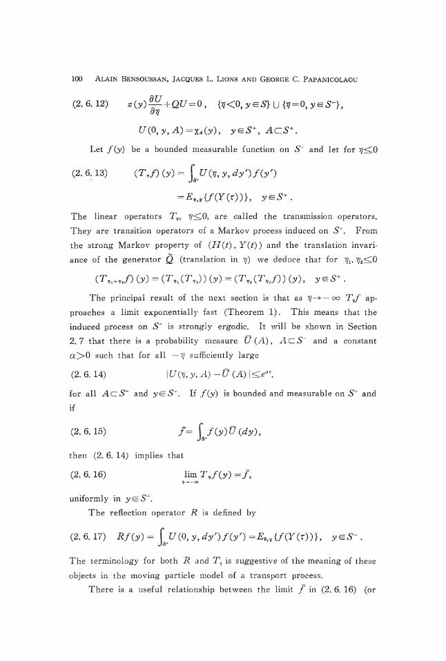
(2.6.12) z(y)?
+, ACLS+.Let f(y) be a bounded measurable function on 5"1" and let for
(2. 6. 13) (T,/) (y) = f £7 (77, y, *y')/(y'JS+
The linear operators T,, ?7<CO, are called the transmission operators.
They are transition operators of a Markov process induced on 5T. From
the strong Markov property of (H(f) , Y(t) ) and the translation invari-
ance of the generator Q (translation in r/) we deduce that for ^, %fSO
(T,I+,,/) (y) = (T,, (T,,) ) (y) - (T,2 (T, ,/) ) (y) , y e 5+ .
The principal result of the next section is that as fj— > — oo Tvf ap-
proaches a limit exponentially fast (Theorem 1) . This means that the
induced process on S^ is strongly ergodic. It will be shown in Section
2.7 that there is a probability measure U (A.) , AdS~ and a constant
a>0 such that for all —f\ sufficiently large
(2. 6. 14) IC/0?, y, A) -C7 (A) |<^a7,
for all AdS4" and ye-5T. If /(y) is bounded and measurable on S^ and
if
(2.6.15) /= f /(y)C7(dy),Js*
then (2. 6. 14) implies that
(2. 6. 16) lim T,/(y) =/,
uniformly in
The reflection operator .R is defined by
(2.6.17) Rf(y)= fJ5*
The terminology for both J^ and T1, is suggestive of the meaning of these
objects in the moving particle model of a transport process.
There is a useful relationship between the limit f in (2. 6. 16) (or

BOUNDARY LAYERS OF TRANSPORT PROCESSES 101
2. 6. 15) and Rf which we shall now derive.
For f(7], y) , a differ eiitiable function of f] and a bounded measurable
function of y, Qf(y, y) is defined by (2. 6. 7) . We now define Q* acting
on /*(??, A), ^<0, Ad S, which are differentiate for each fixed A and
measures for each fixed ~fl as follows:
(2.6.18)
')- fJA
With this notation we have the following Green's identity: for any yi<
and any f fay) such that Q/=0 and /* (y, A) such that Q*/*=0
(2.6.19) 0 = f% f [/*(v,J?! JS
- fJ
Let 7z (v) be a bounded measurable function on *Sf"r and let u ( i ] , y ) be
the solution of
(2. 6. 20) s^l^ + Q^O ? ^<0, ytES} IJ {^ = 0, y eS-}
Let A = lim7_>_00«(T7, y) which is a constant by (2. 6. 16). We apply first
the identity (2.6.19) with ^^O, ^ = — 0 0 to the functions
f*(y,A)=P(A).
This yields the result
(2. 6. 21) f z (y ) (u (0, y ) - A ) P(dy)=0Js
which we may rewrite, using (2. 6. 17) , as
(2. 6. 22) f z (y ) A (y ) P (dy ) + fJs* Js-
Let us apply (2. 6. 19) with % = (), ^ = — 0 x 3 to the functions
* (y ) 1M (y ) P (^) - 0 .s-

102 ALAIN BENSOUSSAN, JACQUES L. LIONS AND GEORGE C. PAPANICOLAOU
Here 0(3', A) is the recurrent potential kernel of Y(t) defined by (2. 5. 8)
where P(t,y,A) is the transition function of Y(f). Clearly this choice
of /* satisfies Q*/*=0 so the identity (2.6.19) applies. We obtain
(2. 6. 23) f *(y) («(0, y) - h) f z(y')P(dy'W(y' , dy) =0 .Js Js
This implies that
(2.6.24) A = ^-f*(y) fsCyJs Js
which, using (2. 6. 17) and rearranging, takes the form
(2. 6. 25)
')r f A(y)*(y)0(y' ,<*y) + f £A (y)*(y)0(y',L Js+ ___ Js-
with the denominator positive by the hypothesis below (2. 6. 6") . This is
the desired relationship between h and Rh.
We turn next to the half-space problem with reflection. The reflected
process (HR (t) , YR ( t ) ) is defined on the state space {(-co, 0] X S} . In
the interior set of points {(— cx^, 0) X /S} |J {{0} X S ~ } 9 the generator is Q,
given by (2. 6. 7) , as before. On the boundary {0} X S+ the process is
reflected instantaneously according to a given probability law B(y,A),
y^S+, AdS~, just as in Section 2. 2. We assume that the kernel B
satisfies condition (2. 2. 9) (x corresponds to the single point ^ = 0 here)
and this insures that the process hits the boundary finitely often in finite
time intervals, with probability one. We denote by PftV and by E*y the
probability distribution and expectation starting at (??, 3*) of the reflected
process.
We consider the solution of the following initial-boundary value prob-
Recall the convention that (2. 6. 26) is taken in its integral equation form.
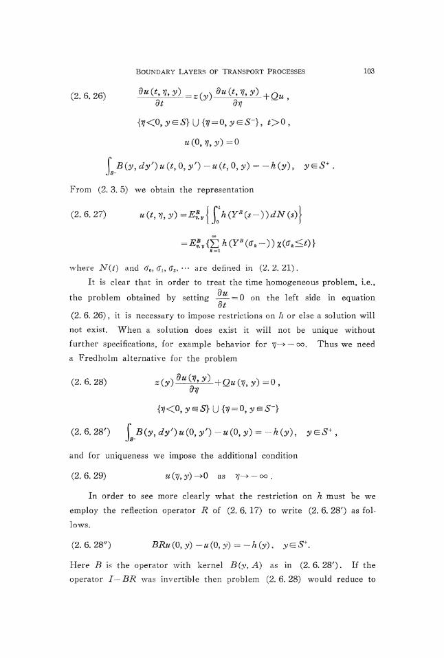
BOUNDARY LAYERS OF TRANSPORT PROCESSES 103
(2.6.26) =z(y) +Qu,dt dy
, t>0 ,
«(0 ,7 ,y)=0
f B(y,dy')u(t,Q,yf)-u(t,Q,y) = -h(y},Js~
From (2. 3. 5) we obtain the representation
(2. 6. 27) u (t, y, y) = £*, { £ h (YR (s-})dN (s) j
where N(t) and <T0, (7^ (72, ••• are defined in (2.2.21).
It is clear that in order to treat the time homogeneous problem, i.e.,
the problem obtained by setting - = 0 on the left side in equationdt
(2. 6. 26) , it is necessary to impose restrictions on h or else a solution will
not exist. When a solution does exist it will not be unique without
further specifications, for example behavior for rj-> — oo. Thus we need
a Fredholm alternative for the problem
(2.6.28) s O v ) M ' y +Q«0? ,y )=o .
(2.6.28') f S(y,^y /)«(0,y ')-«(0,y) = -Js-
and for uniqueness we impose the additional condition
(2. 6. 29) u (77, 30 ->0 as T?-> - oo .
In order to see more clearly what the restriction on h must be we
employ the reflection operator R of (2. 6. 17) to write (2. 6. 28') as fol-
lows.
(2. 6. 28") BRu (0, y) - « (0, y) = - A (y) , y <E S+.
Here .B is the operator with kernel S(y, A) as in (2. 6. 28X) . If the
operator I—BR was invertible then problem (2.6.28) would reduce to

104 ALAIN BENSOUSSAN, JACQUES L. LIONS AND GEORGE C. PAPANICOLAOU
problem (2. 6. 20) with h replaced by (I—BR) ~~lh. However, the opera-
tor BR has 1 as an eigenvalue since both R and B transform the func-
tion one (on their respective ranges) to itself. Equivalently, from
(2. 6. 27)
will not exist (N(£) — >oo with probability^ one) unless h is appropriately
restricted.
The operator BR is the transition operator of a discrete-time Markov
process on S+ and for f(y) bounded measurable on S~ we have
(2. 6. 30) BRf(y} = f B(y, dy') \ U(0, y', dy")f(y")Js- Js-
= f /GO { B(y,dy')U(0,y',dy"-).Js+ Js-
If we assume, as we will do, that there exists a probability measure (f>
on S~ and a 5>0 such that
(2.6.31) B(y,A)>dt(A),
then it follows that BR is strongly ergodic with UR(A), AdS'1', its
unique invariant measure (and the Fredholm alternative holds) , It is
enough to notice that
as a consequence of (2. 6. 31) . The rest goes as in Section 2. 5. In fact
\BR(yi,A)-BR(yt,A)\
S+tVlty2 is the set of y's where B(yl9 A) — B(y2, A) is positive
(Hahn decomposition). Here p — l — B by (2.6.31) as in (2.5.14).
Thus, the relevant ergodic properties for the reflected process can
be deduced in an elementary way from a hypothesis such as (2. 6. 31) .

BOUNDARY LAYERS OF TRANSPORT PROCESSES 105
We require no ergodic or other properties from [7; all is based on the
B. If we know that £7(0, y, A), y^.S~, AC5"1", satisfies a lower bound
like the one for B, then that in turn suffices for the ergodicity of BR
without assumptions on B, other than the ones made before (2. 6. 30).
Note that the invariant measure UB of BR is the asymptotic distribution
of Y*(<T*-) as k-*oo.
Let us return to (2. 6. 28) and assume that
(2.6.32) f UR(dy)h(y)=0.Js+
Then, by the Fredholm alternative and (2. 6. 32),
(2.6.33) « (0 , jO=vj ( (&R)*-C7 B )A(30+6- ,
where (BR)°(y, A) =XA(^) and (BR)k for &>1 are the interates of the
transition operator BR. The sum in (2. 6. 33) converges since (BR)k
tends to UB geometrically fast as k—>oo. In (2. 6. 33) we have also
added a constant c on the right hand side which is to be determined
from (2. 6. 29).
In fact, with u (0, y), ye*ST, determined, problem (2.6.28) is identi-
cal to (2. 6. 20). Thus for each constant c, (2. 6. 28) and (2. 6. 28')
have a unique solution u ( y 9 y \ c ) . From the ergodic properties of
U(ij,y,A) as J]—> — oo (c.f. (2.6.14)) it follows that linv>~oo^07, y\ c)
will exist for each c and we will have
(2. 6. 34) lim u (??, ? ;< : )= ft/ (dy) f] ( (5J?) * - f/B) A (y) -f- c .
If we choose the constant c so that the right-hand side of (2. 6. 34) is
zero, then (2. 6. 29) is satisfied and (2. 6. 28)-(2. 6. 29) indeed has a unique
solution if h is such that (2. 6. 32) holds. The special constant c so
chosen will be denoted ch
(2.6.35) Cfc=
The solvability condition on // for the problem
(2.6.36) s ( y ) - ^ + Q«=-/U,30, r/<0,

106 ALAIN BENSOUSSAN, JACQUES L. LIONS AND GEORGE C. PAPANICOLAOU
«— »0 exponentially fast as fj— > — oo ,
Bu-u=-h, y = 0y y<=S+ ,fJs-
with f— >0 exponentially fast as '(]— > — oo, is the same as above, namely
(2. 6. 32) . However, the constant c must be chosen in accordance with
Theorem 2 of Section 2. 7 (cf . (2. 7. 41) ) and it depends on 7z and /.
2. 78 Potential Theory for the Half-Space Problem
In this section we shall first show that, as ij-* — oo, U(i], y, A) has a
limit U (A) and that (2. 6. 14) holds. Then we shall prove some related
results that will be also needed in the asymptotic analysis of the follow-
ing sections.
Theorem l.f Let U(y,y,A), ^<0, yd 5, AdS~ be the solution
of (2.6.12). Then there is an ??0, — oo<??0<0 and a p<l such that
(2.7.1) \U(^yi,A)-U(7j0,y2,A)\<py yl9y^S9 AdS+.
Remark. From (2. 7. 1) it follows that
(2.7.2) li
exists uniformly in y£iS and, moreover, the limit is approached exponen-
tially fast i.e., (2. 6. 14) holds. The passage from (2. 7. 1) to these re-
sults is as in Section 2. 5.
Proof. Let jP (*, ??, y, D) be the transition function of (H(t) , Y(t) )
whose generator is Q of (2. 6. 7). Here DC {(— oo, 0] XS}. Let tQ be
a positive number to be chosen later and suppose that t0<^ — y0. Let
P (t, y, A), y^S, Ad S, be the transition function corresponding to the
generator Q of (2. 6. 1) i.e.,
(2. 7. 3) P(t, y, A) =P{Y(f) <=A\Y(Q) =y},
and let P (A) , Ac^S, be its invariant measure. From the results of
This theorem is due to S. R. S. Varadhan (private communication).

BOUNDARY LAYERS OF TRANSPORT PROCESSES 107
Section 2. 5 we know that (2. 6. 5) holds. Since £ (3;) in (2. 6. 7) is
not identically zero and since (2. 6. 6) holds, it follows that for some
(2.7.4) P{|z(y)l>0}=r>0.
Let us also choose ta sufficiently large so that
(2.7.5)
as we know is possible by (2. 6. 5) .
We shall need the following general fact about two probability mea-
sures Pl and Pz (on some general measurable space X) .
(i) There exists a measure Ps and two measures JP/ and P2' which
are orthogonal to each other such that
(2. 7. 6) P: = P3 + P/, P2 = P3 + P,'.
(ii) P, (X) = 1 - sup |P, (A) - P2 (A)AC.X
P/ (X) = P,' (X) = sup IP, (A) - P2 (J) 1 .AdX
These facts are verified as follows. Define the signed measure v(A)
on ^Y by
v(A)=P1(A)-Pt(A)
and let 5+ and B~ be a Hahn decomposition for y (A) so that 5+ U £»~
= X, B+n-B~-0, J>(JBTlA)>0, y(^-nA)<0, for all Ac.Y. Now
define
(2.7.7) P3(A)=l(P1(A)+P2(A))-lv(5+pA)+lv( JB-n^).^ £ £
Since v(A) =y (An S+) + v (An S~) it follows from (2.7.7) that
(2.7.8)
Define also
(2.7.9) /Yd) -=v(Bl n A), TV (A) = — v(B~ f] A).
From (2. 7. 8) and (2. 7. 9) il follows that (2. 7. 6) (i) holds and that

108 ALAIN BENSOUSSAN, JACQUES L. LIONS AND GEORGE C. PAPANICOLAOU
PI and P2' are orthogonal. To verify (ii) in (2. 7. 6) we note from
(2.7.8) that
But
Thus, the facts stated in (2. 7. 6) have been proved.
We return now to the proof of the theorem. Let P (tQ, y^ A) and
P(A>3 ;23^) be denoted, respectively, by Pl and P2 on S and let P3 and
PI', PZ be the other measures described in (2.7.6). From (2.7.5)
and (2. 7. 6) it follows that
(2. 7. 10) P8(5) =l-sup |P2 (A) -P,(A) I
and
(2.7.11) P1'(S)=P,'(5)=1-P,(,S)
Note further that
<sup|P,(A)-J
™¥ T~T'
Hence,
(2.7.12) P,{|*(y)|>0}

BOUNDARY LAYERS OF TRANSPORT PROCESSES 109
Now let U(-q,y9A), ??<0, y^S, AdS be the solution of (2.6.12).
If tQ<^ — f]0 i.e., % is sufficiently large and negative, we have
(2.7.13)
= f G (T?O, y,, y3; A) P (£„, y,,i J
where,
(2.7.14)
= E{U(H(t,) , y (^0) , A) ly (*„) =y,, y (0) =y i > H(0) =%}
is a non-negative function bounded by one. Thus, using (2. 7. 6) ,
(2.7.15) \U(7i0>yi,A)-U(Tja,y2,A-)\
= I [GO?,, ylt y3; A)P,(rfy,) - [G(T?O, yf, ys;I J J
J [G 0?», y i, y, ; A) - G (?„, y,, y, ; A) ] P
< J|G(i?,, yi, ys; A) -G(i?,, y,, ys; A) |P3(c?y3)
We must now estimate the integrand on the right of the last inequality
in (2.7.15).
From (2. 7. 14) it follows that
(2. 7. 16)
< sup |J7(^, y&- A)-U(3i, y,; A)\,

110 ALAIN BENSOUSSAN, JACQUES L. LIONS AND GEORGE C. PAPANICOLAOU
where we have used the fact that |c(.y)|<^l. Therefore it suffices to
estimate \U(yly y; A) — £/(%, y\ A) \ and this we do directly from (2.6.
12). We have that
or, upon integrating,
£/(%, y ; A) <C7(%, .y; A) e«".-"."i
and hence
t/Ofc, y, A) - f/(^, v, A) <1 - <r'i'
Replacing U by 1 — £7 in this argument gives
(2. 7. 17) |t7(%, v, A) -C7(^,y, A) l^l-^-
We may also replace g (;y) on the right hand side by qu from (2. 5. 3) .
We return now to (2. 7. 15) and use (2. 7. 17). This yields
(2.7.18)
(by (2,7.12))
4
This completes the proof of the theorem.
We are now in a position to complete the potential theory associated
with the process (H(t), Y(t)) on (— oo, 0] XS and generated by Q of
(2. 6. 7) . We have the following result that will be used in the asymp-
totic analysis.
Theorem 2, Let #0?, y) be a nonnegative function on ( — oo? 0]
X S such that
(2. 7. 19) g (7f v) <r A 7?<0, r>0, S>Q .

BOUNDARY LAYERS OF TRANSPORT PROCESSES ill
Let h(y) be a bounded f IMC ti on on S and consider the problem
(2.7.20) -*(y) + Q w = g , on {?<0, y ^S} U {7 = 0,
(cf. (2. 6. 12)). I/7 7i(y) 75 adjusted appropriately by the addition of a
constant (see (2. 7. 41) below) , then (2. 7. 20) 7z#s <2 unique bounded
solution w(y9y) that decays exponentially fast as y—> — oo.
Before giving" the proof of this theorem we prove a lemma as fol-
lows.
Lemma. Let g ("/?, y) satisfy (2.7.19). Then there exist solu-
tions of
(2.7.21) ~z(y) + Qw=g, on {7?<0, y
lliat are bounded for all
Proof of the Lemma. We shall assume that the solution of (2. 7.
21) that we seek satisfies zc;(0, y) =0, y^.S^\ we show that such a solu-
tion exists and is bounded.
Suppose we can iind a funct ion // (^, y) such that
(2. 7. 22) 0<?/<M<oo
and
(2.7.23)
Then
(2. 7. 24)
and the lemma follows. To see that (2. 7. 24) is true note that for any
we have

112 ALAIN BENSOUSSAN, JACQUES L. LIONS AND GEORGE C. PAPANICOLAOU
(2. 7. 25) oo>M> u 0?, y)
>£, J r*I Jo
>£„,{ fr1 Jo
and hence (2. 7. 24) also, by letting t*[ oo. Here r is the first time
reaches the origin starting from H(G) — <CO.
To construct the comparison function u we proceed as follows. Let
/O?) , ??<[0 be a smooth function to be chosen later on and define fl (y, v) ,
My,v) by
(2.7.26)
Here and in the remainder of the proof of this lemma the overbar denotes
average with respect to the invariant measure of Q i.e., P of (2. 5. 6) .
Clearly /i and fz are well defined because of (2. 5. 9) , (2. 5. 10) and
(2. 6. 6) . We write
(2.7.27) /1=_Q-i*l£
df
The positivity was assumed explicit y below (2. 6. 6"). From these defini-
tions it follows that
(2. 7. 28) - (z-- + Q (/+ /, + /,)
Now choose f(ff) so that
(2.7.29) _ £

BOUNDARY LAYERS OF TRANSPORT PROCESSES 113
with 0 </?<<? and 0<C7<C^ appropriately chosen. With this choice, the
right hand side of (2. 7. 28) , which is h of (2. 7. 23) , is
[ 0/0l_£e^-i
0
For ££ sufficiently large and /?^>0 sufficiently small we achieve the in-
equality on the right side of (2. 7. 23) . Integrating (2. 7. 29) yields
(2.7.31) /(,) = (A -**)>() , 7?<0,6 p
where A>0 is sufficiently large. Moreover if u=f-\-fi~\-fz then clearly
u>0 if A is sufficiently large. This completes the proof of the lemma.
Proof of Theorem 2. Let (T7/)(y) be defined by (2. 6. 13). It
follows from the lemma just proven that we may write the solution of
(2.7.20) as
, Y (
Let z*i, T2, • • • , rn be the first times —/z + 1, — ;z + 2, • • • , 0 are reached start-
ing from f\— —n. Then,
(2.7.33) w(-n,y) =£_B|F{ J^g(H(5), F(j)) A
(2.7.32) zc. (^, y) =• JEM { A (y(r) )}+£„{ [( Jo
Here 2^ is the ^-algebra associated with the stopping time rfc-i. With
define
(2. 7. 34) 5. (y) = £_.,, I f "fir (H (5) , Y (5) ) ds\ .( Jo J
From the lemma above it follows that
(2.7.35)
for some constant c^>0 and <?>0 sufficiently small. From (2. 7. 33) and
(2. 7. 34) it follows that

114 ALAIN BENSOUSSAN, JACQUES L. LIONS AND GEORGE C. PAPANICOLAOU
(2. 7. 36) w ( - n, y) = gn + T^gn^ + Tl ., + • • • + T^fr .
Let Gn(y) be defined by
(2.7.37) G»(y)=I]2f»(y).fc=l
We shall show that
(2.7.38) limw(-n,y)=Gn f o o
where
(2. 7. 39) G = f G (y ) C7 (dy ) , G (y ) = lim Gn (y )JS+ w f oo
and the limit in (2. 7. 38) is approached exponentially fast, uniformly in
y^S. Note that G(y) exists since Gn(y) is an increasing sequence and
the limit G is approached exponentially fast in view of (2. 7. 35) . We
write
(2.7.40)
The second term on the right side of (2. 7. 40) is small uniformly in n
and y as long as k is sufficiently large. With k large and fixed now we
let n—»oo on the first term on the right side of (2.7.40). By the
ergodicity of T_j it tends to
f U(dy}£ (T*_7'gf,) (y) = fJs* .7=1 Js*
and so the statement is proved.
Let h be defined by
= fJs+
If we adjust A(y) by adding a constant so that
(2.7.41) /H-G-0,
then clearly z^(^53/)->0 as ^^ — oo and the approach is exponentially
fast uniformly in y^S. The proof of the theorem is complete.

BOUNDARY LAYERS OF TRANSPORT PROCESSES 115
§ 3. Diffusion Approximations
3. I. Asymptotic Expansion in an Unbounded Region
and Homogeiiization
We begin with the asymptotic analysis as £->0 of the following prob-
lem (cf. Section 2. 4)
/o i i\ du£(t, X. y} 1 ~ £/, N(3. 1. 1) - o * = — Q*,W*(t,x9y)ut S
_
e
(3.1.10 « e (0 ,^y)=
Here F(o:, C 3;) and G(x,^,y) are smooth bounded functions on RnxTfl
X S-~»Rn, where Trt is the unit ^-dimensional torus and S is any compact
metric space (such as the unit sphere in Rn for example) ; a (x, C y) is a
smooth bounded function on RnXTnXS->R. The operator QJiC/ with
parameters x^Rn and ^<^Tn, is given by
(3. 1. 2) Q..C/CV) = v (x, C, y) f TT (^r, C, y, dz)f(z) - q (x, C y)/0v) ,Js
where g is a continuous function on R^X^xS such that
(3. 1. 3) 0<^<<? (x, C 3')
and 7T (x, C, y, A) , A a Borel subset of 5, is a probability measure for
each (#, C> y) °n RnXTHxS and is continuous in (.r, C, 3;) for each Borel
set A. Under these conditions (3. 1. 1) has the probabilistically natural
(generalized) solution
(3.1.4) ,/' (t, .r, y) - ETty fexp ([a (,Yf (.) , ¥&, V (I v Jo £

116 ALAIN BENSOUSSAN, JACQUES L. LIONS AND GEORGE C. PAPANICOLAOU
for bounded and continuous f(x,£,y). Here (Xs (t), ¥*(£)), £>0 fixed,
( V \= —) dependence
£ /of coefficients and data is smooth then if (t, x, y) is smooth also and
satisfies (3. 1. 1) in the usual way. We shall assume that this is the
case in what follows.
We wish to describe the asymptotic behavior of if (t, x, y) as £—»0,
0<£<T<°° and to analyze the corresponding process (Xs (t), Y2 (t)).
To this end, and under liberal smoothness assumptions, we first construct
an asymptotic expansion for if (t, x, y). In Section 3. 2 we prove that
this is a valid asymptotic expansion and in Section 3. 3 we show that
Xs (t), 0<£<T, converges weakly as a process on C ([0, T]; Rn) to a
diffusion Markov process.
Let us introduce explicitly the variables
(3.1.5) C = -, ? = ~£ £2
and let us seek an expansion of the form
(3. 1. 6) «• (t, x, y) = f; e*«t (t, x, C, y)k = 0
Here the superscript IL stands for "initial layer" and reflects the nature
of such terms on the right side of (3. 1. 6) as we see below. We require
that both sums on the right side of (3. 1. 6) satisfy (3. 1. 1) and that
their sum satisfies (3. 1. lx). Thus, we have at first the following se-
quence of problems1 for the interior expansion (uk without superscripts).
(3.1.7)
(3.1.8)
(3.1.9) ^i«^+j:,«y-i+j:,^-,—^2 = 0, #=2,3,4,(J £
Here X\, Xz and Xz are defined by
In inserting (3. 1. 6) into (3. 1. 1) and equating coefficients of equal powers of e, wetreat x, C and £, r as independent variables. Thus, (d/dx)-*(d/dx) + (I/O (d/d£).

BOUNDARY LAYERS OF TRANSPORT PROCESSES 117
(3.1.10) -Ci = Q*,t + F(x,C9y).
(3. 1. 11) £, = F(x, C? y) ~ + G(x, C, y) -
(3.1.12)
We take W0 independent of y and C so that u0 = uQ(t,x) satisfies
(3. 1. 7) . We will find the determining equation for u0 later. We con-
sider next equation (3. 1. 8) . The operator Xi is an operator on func-
tions TnxS with x a fixed parameter. It is precisely of the form (2. 5. 2)
for which we have studied the validity of the Fredholm alternative in
Section 2. 5. The theorem at the end of Section 2. 5 deals with the case
5= unit sphere in Rn and F = y9 this is the case of interest in transport
theory. We shall assume that the Fredholm alternative, as stated in
that theorem, is valid for JC1 of (3. 1. 10) in order to get a better idea
of the structure of the expansion. The remark at the end of Section 2. 5
clarifies the smooth dependence of quantities on the parameter x.
Let P (dyd^\ x) be the invariant measure1" of £lm We shall assume
that
(3. 1. 13) f F(x, C, y}F(dyd^ x} =0 ,Jr«xs
i.e., that the singular velocity term in (3. 1. 1) averages to zero relative
to the invariant measure of the cell-collision operator jClt Condition
(3. 1. 13) and the Fredholm alternative for X\ yield the solution HI of
(3. 1. 8) in the form
(3. 1. 14) MI = «IO— -Cr'-fzHo ,
or more explicitly
(3. 1. 15) Ul (t, x, C, y) = u10 (t, x)
+ f ff (y, C, dy\ dC ; x)F(x, C', yx) • 9gl'(*' .JTnxS Qx
We use ~ to distinguish objects on TnxS from the corresponding ones on S alone(i.e., without fast periodic structure).

118 ALAIN BENSOUSSAN, JACQUES L. LIONS AND GEORGE C. PAPANICOLAOU
Here 0 is the recurrent potential kernel of Xi that is, if P (t, y, £, A; x) ,
AdTnXS is the transition function corresponding to Jll (the kernel of
then,
(3. 1. 16) $(y, C, A; x) = (""[£(*, y, C, A; x}Jo
The function u1Q (t, x) , like u0 (t, x) is determined later.
We use next (3. 1. 14) in (3. 1. 9), with N=2, and rewite it in the
form
i 2 2 1 0 i 2 0 s 0 - ,dt
Let us denote by overbar integration of a quantity with respect to P.
Then the solvability condition for u2 is clearly
(3.1.17) =(-j:i£?£^£^u,=Xu,.Ot
Note that the term — _C2«io drops out upon averaging in view of (3. 1. 13) .
Explicitly the operator X on the right side of (3. 1. 17) has the form
(3.1.18) Xg(x)
= f>
X
-h
fjTnx
fJTnx
This is an elliptic second order differential operator and so (3. 1. 17) is
a parabolic equation for UQ (t, x) . Initial conditions for UQ will be obtained
from the initial layer analysis later.
The solution uz of (3.1.9) (with N=2) takes the form
(3. 1. 19) uz - u20 - XilX2u1Q - Xrl ( - £*£?£* +Xs-I)uQ,
where //20~~ ^20 (^> -0 i-s determined by the solvability condition for (3. 1. 9)
with N = 4. The solvability condition for (3. 1.9) with N=3 determines
(up to initial data) the function u1Q (t, x) as ^ve no^w sho^v. We have

BOUNDARY LAYERS OF TRANSPORT PROCESSES 119
— £zuz — £sUi + -^1
dt
£z l£^
= (£2£l l£2 —
dt
from which we obtain the following equation for u10 (t, x)
dt
This is an iiihomogeneous diffusion equation with inhomogeneous term
depending on UQ. Initial data are determined below from the initial layer
expansion.
The higher order terms in the interior expansion in (3. 1. 6) (not the
initial layer terms) are obtained in the same fashion up to initial conditions.
Each time UN is solved from (3.1.9) an unknown function um(t,x) is
introduced and this is in turn determined (up to initial values) by the
solvability condition for uN+2.
Now we consider the initial layer expansion. Inserting 2*>=o£*M*L
into (3. 1. 1), treating £ and r as independent variables, and equating
coefficients of equal powers of s leads to the following problems.
(3.1.21) ^-
,.
(3. 1. 22) ™±-= £lUlL+£zul9t
(3.1.23)at
We require also that
(3.1.24) ^L(r,:r,Cy)-»0 as r-*oo, 7V=0, 1, 2, •
and, from (3.1. I/), that
(3. 1. 25) «o (0, x9 C, y) + ^oji (0, x, C, y) =/(a:, C, y) ,

120 ALAIN BENSOUSSAN, JACQUES L. LIONS AND GEORGE C. PAPANICOLAOU
(3. 1. 26) UN (0, x, C, y) + *4L (0, x, C, y) = 0, JST= 1, 2, • • • .
Clearly (3. 1. 24) is the condition that we have an initial layer behavior
and (3. 1. 25) , (3. 1. 26) are the initial conditions from which we will
determine initial values for UQ, u10, w2o> ""•
From (3.1.21), (3.1.25) and the ergodic properties of Xi it is
clear that ulL will go to zero* as r-^oo provided we have
(3. 1. 27) «„" (0, x, C, y) =/(*, C, y) -/ (a-)
where,
(3.1.28) /(*) = f F(rfWy ;*)/(*, C,y)JrnxS
and hence
(3.1.29) K,(0, *)=/(*).
Thus, (3. 1. 17) and (3. 1. 29) determine uQ(t,x) completely and similarly
(3.1.21) and (3.1.27) determine u{L = urQ
L (r, x, C 30 completely (with
.r being a parameter in the WQL problem) .
To determine uv (i.e., initial data for u10) and u[L we note that from
(3. 1. 22) and (3. 1. 26) (in operator notation)
(3.1.30) «1"(r) = -e-r«r«1(0)+ [ 'ex^-^XtulJo
TJo
Jo 2 ""2
The last term on the right in (3. 1. 30) goes to zero as r f °° hence, in
order that u[L (r) —>0 as r—>oo we must have
The initial condition (3. 1. 31) for 2tw (t, x) and (3. 1. 20) determine it
completely. Similarly, (3.1.22) and (3.1.26) (JV=1) determine u{L
and it satisfies (3. 1. 24) (exponentially fast). Thus the second terms
in the expansion have been determined. The rest of the terms are calcu-
ulL actually goes to zero exponentially fast as r->°o.
BOUNDARY LAYERS OF TRANSPORT PROCESSES 121
lated by the same general process.
When (3. 1. 1) has no rapidly varying periodic terms, i.e., jc/e does
not appear in JF\ G, a, Q, and f9 then the above expansion yields the
standard diffusion approximation of transport theory [1 and the references
therein]. On the right side of (3.1.1) we do not have terms with y
derivatives (force terms, whenever this makes sense) but the formalism
extends obviously to this case.
3. 2« Validity of the Expansion
The validity of the expansion (3. 1. 6) rests upon the following three
general ingredients which have been mentioned already.
( i) Smoothness
(ii) The Fredholm alternative for J.\ of (3. 1. 10)
(iii) The centering condition (3. 1. 13).
Smoothness is inevitable if we want expansions and error estimates. The
Fredholm alternative for Xi must also hold one way or another; it is the
essence of the expansion procedure. The centering condition (3. 1. 13)
can be removed but then the expansion (3. 1. 6) changes form and in
particular u$ depends on e in a nontrivial way.
The result we state below (and results in other sections to follow)
follows easily from hypotheses of the form (i), (ii), and (iii) above.
The results1 of Section 2. 5 on the Fredholm alternative are not intended
for literal use but to show that (ii) is nonvacuous in the present con-
text. We state the results in some generality assuming that (i), (ii),
and (iii) do hold.
Let us return to (3. 1. 1) and assume that coefficients and data depend
smoothly on x and £. We also assume that
(3. 2. 1) The Fredholm alternative as in the theorem at the end of
Section 2. 5 is valid for Xl of (3. 1. 10).
The coefficients of the diffusion equation (3. 1. 17) being smooth by hy-
potheses and /(.r) being smooth imply that the solution u0(t, x) is also
smooth. Similarly, u*}L is smooth and so on.
T The theorem at the end of Section '2. 5.

122 ALAIN BENSOUSSAN, JACQUES L. LIONS AND GEORGE C. PAPANICOLAOU
Theorem. Under the above hypotheses, the construction of the
expansion (3.1.6) gives an asymptotic expansion of zcs (t, x, y) as £—>
0, 0<£<T<oo, x^Rn, y^S. Specifically, we have that uniformly
N / „ \ JV f f „/ Q O O \ - £ / * \ **.—! _ k I . •A* \ X—! _ Tf. T T; / *" •*'
o \ e / fc=° \e s
Proof. The construction of (3. 1. 6) makes sense since all is smooth.
By construction we have that
- — («•-
and
=01.0 = 0.
By the maximum principle (recall a is bounded and 0<^<CT<C°°) it fol-
lows that
But,
(3.2.3) [« f i
fc=0
This completes the proof of the theorem.
3. 3. Weak Convergence of the Process
Let XB denote the infinitesimal generator of the process (Xs ( t ) ,
Y£ (t) ) , the one associated with (3. 1. 1) :

BOUNDARY LAYERS OF TRANSPORT PROCESSES 123
(3. 3. 1) _£' = [±F(X, £-, y) +G(*. f , y)]
The state space of the process is RnXS, where S is a compact separable
metric space and Qx c, £==—, is defined by (3. 1. 2). The purpose of this£
section is to show that Xs (f) , Q<^t<T<^oo, converges weakly as a meas-
ure on C([0, T]; Rn) as £-»0, to the diffusion Markov process X(t)
whose generator is _£, given by (3. 1. 18) with a=Q. The smoothness
requirements of Section 3. 1 and 3. 2 will be weakened considerably here.
However, we only show weak convergence.
The hypotheses for this section are as follows. Qr.c *s defined by
(3. 1. 2) and q (x, C, y) , n (x, C, y, A) are continuous in (x, C, y) e I?71 X Tra
X-S, have bounded ^: and C derivatives and the Fredholm alternativef
holds, i.e., 0 of (3. 1. 16) is well defined, it is differentiable in x and
takes bounded continuous functions of C? y into bounded continuous func-
tions of C> y. In addition, it maps differentiable functions of C to differen-
tiable functions of C
The vector functions F(x,^,y) and G(x,£9y) are assumed continu-
ous and bounded on RnXTnXS-*Rn and with bounded x and C deriva-
tives. We assume (3. 1. 13) holds.
With these hypotheses, for £>0 JL& of (3. 3. 1) is indeed the genera-
tor of a Markov process as described in Section 2. 1.
Let f(x) be a smooth bounded function and let fl (x, C> 3;) ^>e a bound-
ed solution of
(3. 3. 2) Q,ir/i (*, C, y) + F (x, C, y) • 9 / l C C ' y )
,ox
so that*
(3.3.3) /,(*,C,y)= fJmx
Define J7 on smooth functions by (3. 1. 18) (with <zs=0) or again
As in the theorem ai the end of Section jj. 5 with .y replaced hy F(x,Z,y) (.en para-meter) i.e., (3. 2. 1).<? is defined by (3.1.16).

124 ALAIN BENSOUSSAN, JACQUES L. LIONS AND GEORGE C. PAPANICOLAOU
(3.3.4) Xf(x) = { P(d^dy ; x) \F (x, C, y) • 9/1 (*' C?
Jr»xs L 0.r
We assume that X has continuous and bounded coefficients and that it is
uniformly elliptic.
Theorem. Under the above hypotheses Xs (t) , 0<^<T<C°o, con-
verges weakly as o— >0 to the diffusion Markov process generated by
i.
Proof. First we note [18] that X indeed generates uniquely a
diffusion Markov process on Rn. In addition Xe (t) , £>0, is continuous
with probability one. The proof is in two steps. First we show com-
pactness of Xs in D ( [0, T] ; JR71) and this suffices since Xs and the limit
X are in C [19 p. 150]. Second we identify the limit processes by
showing that they solve the martingale problem associated with X [18].
Since the latter has a unique solution under our hypotheses the proof is
complete.
Let f(x) be a smooth function and define /: by (3. 3. 3) . Put
(3. 3. 5) r (x, :, y) =/ (x) + £/; (x, C, 30 -
It follows that
(3.3.6) £'f'x,^,y=Xf(x)
where
(3. 3. 7) A, (x, Z,y-)=F (x, C, y)
. C, y) - l ' ' +G(x. C, y)9C ^
Thus, ^-l/ (a:, C> 3') is a bounded continuous function on RnXTnxS and

BOUNDARY LAYERS OF TRANSPORT PROCESSES 125
(3. 3. 8) fJmxi
Define M} by
(3. 3.9) Mef(t) =J
From the analysis of Section 2.1 it follows that M}(t) is a bounded
right-continuous, zero mean martingale relative to £Ff, the (T-algebra as-
sociated with the process (Xs (•) » Y5 ( ' ) ) up to time t. The increasing
process1 (M}(t)y associated with this martingale is given by
(3. 3. io) <M; (o > = f ' [.£• Cf ) 2 -JO
xe
= [Q/f - 2/: Q/J Xf (,) , y (*) ds
where we have omitted subscripts on Q for simplicity. The second equa-
lity here follows from the fact that the derivative operators in £* are
of first order and cancell out. Also, the factor £~2 in front of Q cancells
with the £ factors in f5 =/+ £/i since Qf= 0 (/ is independent of y and
o.The increasing process (Mf (fy )> is defined by the condition that
(Mf(t))* — (Mf(t)y be a martingale also. It can be verified by direct
computation that the expression (3. 3. 10) satisfies this definition. We
also have that
(3.3.11)
Let us rewrite (3. 3. 9) using (3. 3. 5) and (3. 3. 6). We obtain
(3. 3. 12)
f For simplicity we write <(M/> instead of <(M/, M/).

126 ALAIN BENSOUSSAN, JACQUES L. LIONS AND GEORGE C. PAPANICOLAOU
/ L \ ' £ ' / *\
£o
Let us also give an explicit expression for Hf in (3. 3. 10) . It is easily
seen that, in fact,
(3.3.13) H,(*,C,:y)=<K*,C,y
x [ f [<?(£, y', d?dy"-,x) -<?(C, y, rfC'^y*;I JTnxS
and this is a bounded and continuous function of its arguments.
Now we go to step one of the proof: weak compactness of ^£ in
D. We choose f(x) to be xi9 i = l, 2, --,n, the coordinate functions suc-
cessively. These functions are unbounded but /j, J?£/~> Af and Hf are
bounded. Let
(3.3.14) bi(x)=Zxi, f = l,2, • • - , 7 7 ,
so that the vector function b (x) is the drift of the diffusion operator X.
From (3. 3. 12) we obtain
(3.3.15) XKO=*<
where Mf (t) and At(x,^,y} stand for A// and A/ with /(.r) =^. De-
fine:
(3. 3, 16) %\ (0 - .r, + f'ii (.Yf (5) ) -h M? (0Jo
r£
+Jo

BOUNDARY LAYERS OF TRANSPORT PROCESSES 127
Comparing (3. 3. 15) and (3. 3. 16) we conclude1 that
lim P{ sup \X£(t) ~Xe(t) |>ff} =0,e I o
Thus, it suffices to show that the processes Xs (t) are (relatively) weakly
compact in D.
We note first that
lim sup P{ sup \Xe(t) \>N} -0#t°° o<e<i
making use of Kolmogorov's inequality for the martingale M\ (f) and
(3. 3. 10) , (3. 3. 11) . It suffices now [19, 20] to show that
(3. 3. 17)
where C is a constant independent of s, £T, t and s. However, from
(3. 3. 14) we have
(I r*t \
%,(3. 3. 18) E{\X£(t) -X*(s) |2|ff.}<4£ J|
+ 4E
5), C a constant.
This clearly implies (3. 3. 17) and the first step (compactness in D) has
been shown. Only the martingale estimate in (3. 3. 18) requires elabora-
tion. We have
E{\M'(f) -Me(s) |2|£FS} = E{(M\(t) -M\(s)Y\3s}
x*
kl'= S a:!.

128 ALAIN BENSOUSSAN, JACQUES L. LIONS AND GEORGE C. PAPANICOLAOU
the last being a consequence of the boundedness of H^ £ = 1,2, --,n.
Step 2, the identification of the limit, is an immediate consequence of
(3. 3. 12) once we show that
(3. 3. 19) lim Ee j O
\'E\A,Js (
for each / smooth and bounded. This is so because (3. 3. 12) and (3. 3.
19) imply that for any limit measure of the processes Xs, the expression
is a martingale. Since the martingale problem associated with X has a
unique solution the proof is complete.
To prove (3.3.19) it suffices to show that for each x^Rn and
uniformly in y
(3. 3. 20) lim Ex>y\ ^24° ' ( Jo
The function Af(x, C, 30 is bounded and continuous. If it were a smooth
function of x and C then (3. 3. 20) would follow immediately in view
of (3.3.8) and the Fredholm alternative for Q + F- — . That is, we
would be able to construct a function Bf(x> C y) (analogous to u2 in
(3. 1. 19)) such that
(3. 3. 21) QX),
and then apply (3. 3. 9) with f = e*Bf.
Since Af is merely continuous in x and C we first approximate it by
a smooth function of C f°r each x and y. Call it AJ so that
(3. 3. 22) Af (x, C, y) ~ A«f (x, C, .v) I
for all (x, C 3') R^XT^XS, Put
(3. 3. 23) Aaf (x) = > (d^dy ; x) A°f(x, C, y ) .
The function Aaf — Aa
f is smooth in C and satisfies (3.3.8). We now
approximate this by a smooth function of x uniformly on compact .r-sets
(without altering (3. 3. 8) ) :

BOUNDARY LAYERS OF TRANSPORT PROCESSES 129
(3.3.24) \Aaf-A
a,-AJ*\<(i
we have
(3. 3. 25)ft
A,dff\Jo
E -f- A1}-
-4- U * _ i l l f p j
A?rf(7 -fl £i j 1 I ( Jo
The first and third terms on the right side of (3. 3. 25) are small if a is
small because of (3. 3. 22) and the fact that A?->0 as <2->0 by (3. 3. 8).
With a fixed the second term on the right in (3. 3. 25) is small for ft
small because of (3.3.24) and the fact that Xs (t) , 0<£<T, stays in a
compact set uniformly in e with high probability (compactness) . With
ct and ft fixed the last term on the right side of (3. 3. 25) goes to zero
as £— >0 because A"'^ is smooth and (3. 3. 8) holds for it. The proof of
the theorem is complete.
3, 4. Boundary Layer Coordinates
In the next sections we shall be concerned with boundary value
problems associated with J?£ of (3. 3. 1) "without ^— dependence, i.e.,
(3.4.1) X'=^Qf+-F^x,y-)-j- + G(X,y)-j-£" S OX OX
where Qx is defined as in (3. 1. 2) but without ^ dependence. It will be
necessary to express the operator JLZ in convenient local coordinates near
the boundaries which are always in .r-space. We do this in this section.
Let 3) be a bounded domain in R" and dW denote its boundary
which we assume is a smooth (;z — l) -dimensional hypersurface. Since the
surface Q3) is a compact subset of Rn it can be covered by a finite
number of open sets that include a d neighborhood of the boundary (i.e.,
U S(x,d), S(x, d) = {y: \x — y\<^.8\) . These finitely many open setsxE.d$will be referred to as coordinate patches.
In each coordinate patch the surface is given parametrically by £
= £(T), $ a vector in Rn and 7= (ft, • • • , 7 n _ 1 ) is the parameter point that

130 ALAIN BENSOUSSAN, JACQUES L. LIONS AND GEORGE C. PAPANICOLAOU
runs over a subset of Rn~l with compact closure. We shall confine at-
tention to a single coordinate patch.
We introduce new coordinates, the stretched coordinates, x— > (ft e^)
given by1"
(3.4.2) *
where for each x in the patch £(7) is the (unique since x is near enough
to the surface) point on the surface such that $ (f) —x and n (f) , the unit
outer normal at $ (f) , are parallel. The parameter j runs over a subset
of I?71"1 and TI<S$ (the lower bound of f] goes to — oo like 1/e) .
We assume that (ft, ft, • • • , fti-i) are orthogonal curvilinear coordi-
nates for g(f) that is
(3.4.3)
are orthonormal vectors that span the tangent space of the surface at
f (f) . The functions 0^(7"), z" = l, • • • , « — ! are the scale factors of the local
coordinates on the surface. Note that (a\a2, ••',an~\n) is an orthonor-
mal frame in Rn at each point of the surface. Define also the curvature
matrix
(3.4.4)
and write
(3. 4. 5) a(r) = (av(r)) = fe(r)^) f, j = l, 2, -, TZ-I
(3. 4. 6) J" (r, T7) = (I-er/a~2p) "'a'1, 1= (n-l) X (rc-1) identity.
The elements of this (w — 1) X (w — 1) matrix are denoted by Jfjt
It is easily seen that in the new coordinates (ft 577) , x-derivatives
are expressed as follows
(3.4.7) 1
Here np and alp are the pLh Cartesian coordinates of the vectors n and
T We shall abuse notation by writing £(#) and n(x) instead of ^(T*(^)) andwhen we want to return from (7-, etf) to x.

BOUNDARY LAYERS OF TRANSPORT PROCESSES 131
a£ /" = !, 2, - • - , ; / —1. The operator J'c of (3.4.1) takes the following
form in terms of the boundary layer coordinates (7% £7?) .
(3.4.8)
11 \—p=i L e
From (3. 4. 8) we see that
(3.4.9) X k - ~ ^ L i - £ i 2 ^ 3 L 4£2 £
where £%L4. is defined by (3. 4. 9) and has coefficients proportional to £.
Comparing (3. 4. 8) and (3. 4. 9) we obtain the following expression for
the operators JLBJA, XBLI and JLBL% in (3. 4. 9) .
(3. 4. 10) JCBLl = Qf (r)
+ i. (f (r) , y) ZP (r) -*=i
(3.4.12) £BL,
-9??
132 ALAIN BENSOUSSAN, JACQUES L. LIONS AND GEORGE C. PAPANICOLAOU
Here Qj denotes the operator Q of (3. 1. 2) (without C dependence) with
its coefficients differentiated with respect to xp, Q%q denotes differentiation
of the coefficients with respect to xp and xq and Fpiq, etc., denotes the
derivative of Fp with respect to xq.
30 5* Asymptotic Expansions for Absorbing Boundary Conditions
(without cells)
In this section we shall analyze the asymptotic behavior as £— >0 of
the following problem. Let 3)c.Rn be a bounded open set with smooth
boundary dS). Let us(x,y) satisfy the boundary value problem
(3. 5. 1) j;sus(x,y) +f(x,y) = 0, {x$E$),y^S} U
(3.5.2) u'(x,y)=g(x,y),
(3.5.3) x ,e2 e dx
(3.5.4) S+ = S+(x) = {y(=S:F(x,y) -n(
Here n (x) is the unit outer normal at x^.dS), /, Q and a are smooth
functions on Rn X S, F (x, y) is a smooth /z-vector function on Rn X S (S
is a compact metric space as in Section 3. 1; for example the unit ball in
Rn) and Qx is given by
(3. 5. 5) O/Cy) = q (x, y) J/r (x, y, dz)f(z) - q (x, y)f(y) .
We assume that q and TT depend smoothly on x, that they are continuous
in y and that (2. 5. 3) and (2. 5. 4) hold (uniformly in x) so that the
Fredholm alternative holds for Qx in the form (2. 5. 9) , (2. 5. 10) . Note
that in (3.5.3) the term G -- (cf. (3.1.1)) has been dropped fordx
simplicity; otherwise S+ depends on e. Also we focus attention on the
time-independent, steady, problem (3. 5. 1) in order to avoid problems
with initial-boundary layers, i.e., difficulties near space-time corners where
special considerations are necessary in constructing complete expansions.
The weak convergence result of Section 3. 3 handles the stopped pro-
cess Xs(t/\ts), ts = first exit time of Xs (/) from 3), under appropriate
conditions. We seek here to analyze, in addition and in more detail, the

BOUNDARY LAYERS OF TRANSPORT PROCESSES 133
behavior of Y2 (f) near <jS) i.e., boundary layer phenomena. That is why
we focus attention on (3. 5. 1), (3. 5. 2). We shall not consider here the
analogous problem with cellular structure.
We begin by looking for an expansion of the form
(3.5.6) u*(x,y)
— Z] £kUk(x, y) +Zj £kukL(y, fC^O, 30 * = ((*-£(*))•»(*))/«&=o &=o
where u^L are the boundary layer terms and they are functions of the
local boundary layer coordinates (cf. Section 3. 4). We assume that out-
side a fixed neighborhood of the boundary ?/fL=0, £ = 0,1,2, • • • . Since
the boundary layer terms, it turns out, decay exponentially away from the
boundary this is easily accomplished by a smooth truncation. On the
other hand it is convenient to have ifkL (??, $ (f), y) defined for all ?7<0
and so we shall allow this mild inconsistency in the following to avoid
complicating the formulas with cutoffs.
The construction of the expansion is as follows. In the interior of
3) we require thai
This yields the following problems.
(3.5.7)
Here we have
(3.5.8) . ,dx
From the ergodic properties of X\ it follows that ICQ = UO(X) i.e., it is
independent of v and the first equation in (3. 5. 7) is satisfied.
Let P (A; x) , AdS be the invariant measure associated with the
process whose generator is Qx of (3. 5. 5) (x is a parameter) . Define,
as in (2. 5. 8) , the potential kernel

134 ALAIN BENSOUSSAN, JACQUES L. LIONS AND GEORGE C. PAPANICOLAOU
(3.5.9) 0(y,4;a;) = f°° [/>(*, 3>, A', x) -P(A- x}~\dt,Jo
where jP(£, y, A; j;) is the transition function. In order to solve the
second equation in (3.5.7) we assume (as in (3.1.13)) that
(3. 5. 10)
Then, by the Fredholm alternative
(3.5.11) UI = UK-£IIJ:.UI,
or
Js dx
As in Section 3. 1, UQ(X) and uw(x), etc., are determined from solvability
conditions for uz and us etc., in (3. 5. 7).
Substituting (3. 5. 11) into the third equation (3. 5. 7) we obtain
(3. 5. 13) Xi«, + j:2 ( «10 - -Tr1 JT,«O) + ^3^o -h /== oand therefore the solvability condition for (3. 5. 13) yields the following
equation for UQ (x) .
(3. 5. 14) Iu0 (x} + /Or) = 0 , x e ^) ,
where
(3.5.15)
(3.5.16) /(^)
Boundary conditions for u$(x) are obtained from the boundary layer ex-
pansion later on. Note that ulQ drops out of the solvability condition
for (3. 5. 13) in view of (3. 5. 10) .
It is easily seen, exactly as in Section 3. 1, that uw(x) satisfies an

BOUNDARY LAYERS OF TRANSPORT PROCESSES 135
equation of the form (3. 5. 14) also. Now the inhomogeneous term de-
pends on UQ(X) however. So, up to boundary conditions, UQ(X) and
WioOe), hence Uj(x,y), are determined. The higher order terms go the
same way.
Let us next consider the boundary layer terms (3. 5. 6). We employ
the notation of Section 3. 4 systematically. It is required that
(3. 5. 17) <£BL(Y\ £ku%L) =0 ,fc = 0
(3. 5. 18) u%L-*Q as ??-> - oo, k = 0, 1, 2, - - - ,
and
(3. 5. 19)
^3.5.20) {uk-rukj\xed£ — *
Since XBL m (3. 4. 9) stops with £BL± we shall stop here with u%L\ fur-
ther computations require expanding XBU and they are not particularly
revealing. Now from (3. 5. 17) and (3. 4. 9) it follows that
(3. 5. 21)
(3. 5. 22)
(3. 5. 23)
Let us look in detail at the determination of u$L. We have that,
with T a parameter (or $ = $(3;), x a parameter)
(3. 5. 24)
(3. 5. 25)
(3. 5. 26)
This is exactly the problem we analyzed in Section 2. 6, specifically, equa-
tion (2. 6. 12) . In order that (3. 5. 24) - (3. 5. 26) have a solution, which
will be unique, it is sufficient that
njs+

136 ALAIN BENSOUSSAN, JACQUES L. LIONS AND GEORGE C. PAPANICOLAOU
where U is the invariant measure of the transmission operator (cf. (2. 6.
15)) and now depends parametrically on the boundary point $ (?'). It
follows that the correct boundary condition for UQ(X} , x^dS) is
(3. 5. 27) «„ (*) ! feta = f U (dy; x) fir (x, y) | ,6W .JS+
Equation (3. 5. 14) and boundary condition (3. 5. 27) determine UQ(X)
and then (3. 5. 24) - (3. 5. 26) determines u%L. Thus, the first term in the
expansion (3. 5. 6) is completely determined.
To solve the equation (3. 5. 22) so that (3. 5. 18) holds for u%L we
use Theorem 2 of Section 2. 7, which was obtained expressly for the
present situation. The quantity XBLZ^L is exponentially decaying as —>
— oo and if u1Q is chosen appropriately at the boundary d£D (cf. (2. 7. 41))
then, Uj_ (x, y) and ufL (y, <? (?), .y) are uniquely determined. Identical con-
siderations lead to the determination of uz and ujL.
Theorem. Assume that F, Q, f, g, <z<CO, depend smoothly on
x^EiS) and continuously on y£=S, that dS) is smooth and that Ju of
(3. 5. 15) is uniformly elliptic in S). Assume that Q satisfies hypo-
theses such as (2. 5. 3) and (2. 5. 4) {uniformly in x) so that it is
ergodic. Assume that (3. 5. 10) holds. Then the solution if (x, y)
of (3. 5. 1), (3. 5. 2) satisfies'
(3.5.28) sup supx^Q y!=S
= 0(e).
Proof. First of all since X is uniformly elliptic and everything is
smooth so is uQ(x)9 the solution of (3.5.14) and (3.5.27). All other
quantities that figure in the above construction are also smooth.
Let
(3. 5. 29) W (x. y) = if (x, y) - (MO (x) + £«, (x, y) + £2«2 (x, y) )
- («f (y, $ (x) , y) + eup (11, f (x) , y)
+ £2«f (-/?, ? (.r) , y) ) |,= ((I-fW).SW)/c •
Recall the convention about cutoffs for «fL stated below (3. 5. 6).

BOUNDARY LAYERS OF TRANSPORT PROCESSES 137
By construction we have that
(3. 5. 30) j:eW*(x,y) =O(e) in {x^3),y^S\ U {
Thus, if a(x, y)< — (J<0 then (3.5.28) follows immediately from
(3. 5. 30) and (3. 5. 29) . If on the other hand we have
(3.5.31) Ec{r£}<c<oo ,
where
(3.5.32) r =
then again the result follows. Here XB (f) has generator s~2Qx-\-e"1F
-- 1 The proof is complete in view of the following.dx
Lemma, Estimate (3. 5. 31) 75 true under, in fact, weaker hy-
potheses than the present ones, provided s is sufficiently small.
Proof of the Lemma. Let X(t) denote the limit process with gen-
erator (cf . (3. 5. 15) )
(3.5.33) Zh(x)= fJS
, f 7 \-ns \— ~ 0(y, dz; x)F(x, z)dx \ dx '
Let r be the first exit time of X(t) from 3). From the uniform ellipti-
city of JC (which is an unnecessarily strong hypothesis) it follows that
there is a function V(x), .rEE.2), bounded smooth and positive such that
(3.5.34) £V(x)<-l.
But then

138 ALAIN BENSOUSSAN, JACQUES L. LIONS AND GEORGE C. PAPANICOLAOU
or
and hence, letting t t oo,
(3.5.35) E*{r}<sup F (*)=<; <oo .x^S)
For example, we may take V '(x) =K—eaXl with K and a sufficiently
large.
With V(x) so defined, define Vl(x,y) and Vz(x,y) by
QxV,(x, y) +F(x, y) . = 0OX
Q,V2 (x, y)+F (x, y) • Z^l - JF (*) = 0 .
Clearly V1 and Vz are well defined bounded and smooth. Furthermore
X-N . JL J-~\ (
It follows that for £ sufficiently small V* = V-\-^Vl-±^Vz is nonnegative
and, say,
, ,2
This implies (3. 5. 31) the same way (3. 5. 34) implied (3. 5. 35) . The
proof is complete.
3. 6, Asymptotic Expansion for Reflecting Boundary Conditions
(without cells)
In this section we shall analyze the asymptotic behavior as e— »0 of
the following problem. Let S)c.Rn be a bounded open set with smooth
boundary dS). Let ite (x, y) satisfy the problem (cf. (2.3.4)).
(3.6.1) .TV(*,
(3. 6. 2) f B (x, v, dz) iC Cr, ~) - if (x, y) + eb (x, y) us (x, y)Js-

BOUNDARY LAYERS OF TRANSPORT PROCESSES 139
(3.6.3) -C* = Q* + -F(x9y)-2-+a(x,y),£- £ OX
(3. 6. 4) S± = SJ- (x) - {y e 5: F (x, y) • ft (x) SgO, x e d£)} ,
(3. 6. 5) a (X y) < - a<0, b (or, y) <0 .
As in Section 3. 5 we do not have — dependence, Qx is as defined in£
(3. 5. 5), n(x) is the unit outer normal to dS),f, g, a and b are smooth
functions on Rn X S and F is a smooth //-vector function on I?" X 5 such
that
(3. 6. 6) f F Cr, y) P (dy ; x) ^0 .Js
Here P(A;.r), Ac*S, is the invariant measure of the process associated
with Qx\ we assume as in 3. 5 that it is ergodic and the Fredholm alterna-
tive holds in the form (2. 5. 9) and (2. 5. 10) . Note that g is multiplied
by £ in (3. 6. 2) . This is the appropriate scaling so that ne = O (1) as
£->0; otherwise if 0r = O(l), then 1^ = 0(8'^.
We need the following assumptions on the boundary operator B (cf.
(2. 2. 9) and (2. 6. 31) ) .
(3.6.7) B(x,y,A), x^dS), yeS", Ac5~ depends1 smoothly on x,
is continuous in y and given (5i^>0 there is a d2^>0 such that
infx^dij) ]/(ES
inf 1]/(ES+ Jn--?
(3. 6. 8) There is a nontrivial reference probability measure (p on S
and a £3>0 such that <?(A)>0 if B(x,y,A) =1 and
for all x^d3), y^S\ Ac:S'.
Under the above hypotheses (some of them are needed only for the
asymptotics) (3. 6. 1) and (3. 6. 2) have a unique solution. Notice the
necessity of having (3.6.5) here; the problem with a = b = 0 does not
have a solution for general / and g.
We begin by looking for an expansion of the form
(3. 6. 9) ue(.r, v) =f] cVCt, v) +f] s*af'(?, f (.r), y)L((,_f(,„.«„,/,*: = 0 fr-0 I
That is, B(x,y,Ar\S~), AdS, is smooth in ~r.

140 ALAIN BENSOUSSAN, JACQUES L. LIONS AND GEORGE C. PAPANICOLAOU
where u%L are the boundary layer terms and they are functions of the
local boundary coordinates (cf. Section 3. 4) . We assume as in 3. 5 that
they vanish outside a fixed neighborhood of dS). On the other hand
it will be convenient to disregardf this in the computation and suppose
that they are defined for all ??<IO; it turns out they decay to zero ex-
ponentially fast as f]-^ — oo.
In the interior, the expansion goes exactly as it did in Section 3. 5,
i.e., we have (3. 5. 7) - (3. 5. 16) . In particular, UQ(X) satisfies (3.5.14)
with X and / given by (3. 5. 15) and (3. 5. 16) .
Let us consider the boundary layer terms in (3. 6. 9) . It is required
that
(3.6.10) JTkCIl 6*^=0,fc=0
(3.6.11) HJ?L-»0 as 7y->-oo, £ = 0, 1,2, • • - ,
(3.6.12) fJs-
(3. 6. 13) f B (Ul + z*fL) - (u, + u^} + b (u0 + UB,L) 4- g = 0 .Js-
The operator J^eBL is given by (3. 4. 9) and, as in 3. 5, we shall not
expand it beyond £BL* so that we stop here with the term UBL. We have
clearly that
(3.6.14) XBL^L = O
(3. 6. 15) XBL^ + £BL^L - 0
(3. 6. 16) -CaLittf* + -Cawttf* + XBuUB,L = 0 .
From (3.6.14), (3.6.11) with & = 0, and (3.6.12) with k = 0 we con-
clude that*
(3. 6. 17) «?L^0 .
Thus, UBL (TJ, $ (x) , y) satisfies the problem (£ (x) a parameter)
r We adopt again the convention about cutoffs stated below (3.5.6).* This means that boundary layer terms are O(f) and should be contrasted with the
absorbing case (Section 3. 5) where they are O (1).

BOUNDARY LAYERS OF TRANSPORT PROCESSES 141
(3.6.18) JTazX^O, 77<0,
(3. 6. 19) z/fL-*0 as 11— > - co ,
(3.6.20) { Bu?L-u?L=-g~ { Eu^i^-bu,,Js- Js-
77 = 0, .v
But this is exactly problem (2. 6. 26) (with ?(x), the point on the bound-
ary, a parameter here) . Hence, the solvability condition on the right
side of (3.6.20) is now as follows (with x = ^(x)
f o/ ^7 \ f / / j f \T?f f\ du0(x)l AB(x,y,dz) <J}(z,dz ;x)F(x,z ) • °v y =0.Js- J-s 9^: J
This gives the following boundary conditions for u0 (
(3.6.21) B(x) .u'* +b(x)u*(x) +g(x} =0 , xdx
where
(3. 6. 22) B (X) = §sUR (dy ; x) [ £0 (y,dz; x) F (x,
- \B(x,y,dz) \<t,(z,Js- Js
(3.6.23) b(x)= f UR(dy;x)b(x, y) ,Js*
(3.6.24) g(x)=
Equation (3. 5. 14) and the boundary conditions (3. 6. 21) determine
UQ(X) uniquely (formally). Note in particular that the term
(3.6.25) 3(*)= \P(dy;x)a(x,y-)JS
in (3. 5. 15) is strictly negative by (3. 6. 5) and this is used in the unique-
ness. We need however one more condition in order to have (rigorously)
existence uniqueness and smoothness of solutions for (3. 5. 14), (3. 6. 21).
This is the following.

142 ALAIN BENSOUSSAN, JACQUES L. LIONS AND GEORGE C. PAPANICOLAOU
There is a 04>0 such that
(3. 6. 26) n(x)-B (x) >S, for all x e dQ .
It is clear that n (x) -B(x)>0 but we must, as we do, exclude tangential
reflection at the boundary.
Returning to (3. 6. 18) - (3. 6. 20) we see that u?L is now uniquely
determined and has the required properties; in particular (3. 6. 19) holds
exponentially fast. The determination of u%L with the right properties
follows in a similar manner. Now however we must use (2. 6. 36) which
relies on Theorem 2 of Section 2. 7. From the solvability condition for
u%L we obtain boundary conditions for uiQ, as usual.
Let us consider briefly the form of the vector field B (x) in (3. 6. 22) ,
in the important special case that
(3.6.27)n(x)-F(x,y)P(dy,x}
This corresponds, of course, to a special choice for the operator B(x,y,
A) . It says, loosely, that reflection at the boundary does not alter the
interior equilibrium distribution of velocities (for a moving particle mod-
el) . If B(x,y, A) satisfies
(3.6.28) f fi(x-)-F(x,y)F(dy;a:)B(x,y,A)Js-
+ {n(x)'F(x9y)F(dy9x)=09 for all AdS~ ,JA
then indeed (3. 6. 27) follows. For this we make use of the identity
(3.6.29) f *(x)-F(x,y)U(0,y,A;x)F(dy;x-)Js-
')=Oy for all
where U(fj,y,A\x) (x^dS) is a parameter) satisfies (2.6.12) with
z (y) == n (x) • F (x, y). Recall also that UB is the invariant measure of
the transition operator BR of (2. 6. 30).
Using (3. 6. 27) in (3. 6. 22) we find that B takes the form

BOUNDARY LAYERS OF TRANSPORT PROCESSES 143
(3.6.30) B(x)= f {JS JS
On comparing (3. 6. 30) with the differential operator in (3. 5. 15) we see
that B (x) is the conormal vector field associated with X. Thus, if
(3. 6. 27) (or (3. 6. 28) ) holds then (3. 6. 21) becomes
(3. 6. 31) du*(& +b(x) u*(x} +g(x) -0 , x(=d£) .dn-j
Theorem. Assume that F, Q, a, B, b* f and g depend smoothly
on x^S), that dS) is smooth, that (3. 6. 5) , (3. 6. 6) , (3. 6. 7) , (3. 6. 8)
and (3. 6. 26) hold. Assume that X of (3. 5. 15) is uniformly elliptic
in 3) '. Assume that Qx of (3. 5. 5) satisfies the Fredholm alternative
hi the form (2.5.9) and (2.5.10). Then
(3. 6. 32) sup sup | u£ (x, y) -u*(x) = O (e) ,x^s) 7/es
where uQ(x) satisfies (3.5.14) and (3.6.21).
Proof. First we observe that our hypotheses imply that tiQ(x) is
smooth along with all other quantities that enter the constructions above.
Define, up to cutoffs,
(3. 6. 33) Wc - if ~ (//o + gw, 4- £2z/2) - (eu*L + fr$L ) .
By construction we have that1
(3.6.34)
(3.6.35)
We must show that this implies
(3.6. 36) M^|=O(s),
from which (3.6.32) follows immediately (cf. (3.2.3)).
Let hi (x, y) and h\ (x, y) denote the right hand sides of (3. 6. 34)
and (3. 6. 35) so that h{ = O (s) and h\ = O (s3) . From the considera-
tions leading from (2. 3. 4) to (2. 3. 5) we conclude that if (Xs (t) ,
Y2 (f) ) is the reflected process generated by
1 We employ the obvious operator notation (cf. (3.6.1), (3.6.2)).

144 ALAIN BENSOUSSAN, JACQUES L. LIONS AND GEORGE C. PAPANICOLAOU
(3.6.37) £
B—I, xG.dS) , y^S+, (instantaneous reflection)
then, (cf. (2. 3. 4) , (2. 3. 5) , (2. 3. 6) )
(3. 6. 38) W (x, y) = £f., { £" A' (5) AJ (X* (j), y* (j)) Js
+ £?. J f"A' (s) AS (X' (*), Y>(s -)) rftf' (,) 1,( JO J
^L£ (0 - exp { ['* (X£(5), 7£(5) ) ds
+ flogf . l
Jo \ 1-^(^(5) y£(5-)Here N2 (t) is the increasing process that counts returns to the boundary
and it is defined as in (2. 2. 21). Note that by (3. 6. 5) the first integral
on the right side of (3.6.38) is indeed O(s). The second integral is
majorized by a constant times
(3.6.39) y£Crs;y)=£3£? J [°°e'n9dN6(s)\, a>09I Jo )
2 B I f *
~Y™£ ' ' " [ J O *
The lemma that follows shows that
(3. 6. 40) ve(t, x, 3>) =j££ J (V( Jo
is bounded independently of x, y, t and e. This completes the proof of
the theorem.
Lemma. Under the hypotheses of the theorem, Vs (t, x, y) defined
by (3.6.40), is bounded independently of t>Q, x^£D, y^S, and
0<£<£0, with a>0 fixed.
Proof of Lemma. Since dS) is smooth there exists a function <t>(x)
on 3) such that 0(.r)>0 for x^3), (f>(x) is smooth and bounded, <f)(x)
= 0, x^dS), and \V(j)(x) \>1, x^d3). For example, for £>0 sufficiently
large, the solution of
BOUNDARY LAYERS OF TRANSPORT PROCESSES 145
satisfies these conditions.
With (fr(x) so fixed we define fa(x,y) as a bounded solution of
(3.6.41) Q,01(x,ya;
This function fa is well defined by the Fredholm alternative for Qx and
(3.6.6). We define 0fL (??, x, y) , x^.d3) as the solution of
as ??— > — oo
77=0 f f f .<IJS*
ES+ 9.r I
We also define1
u * \^ s
11 follows thai
(3.6.43) (^Q, + ±F-^4s = F.^+sfaL-±.
= 0(1)
and
(3. 6. 44) (B -1) L^ - - sB • -^-
We now use the above in (2. 2. 20) to obtain the following identity
(with Xe = s-2Q+£-1F-—).\ Sir
(3. 6. 45) JE£ 77 {^~"V^£ C^f (0, ir<F (0)}
r -as R
Jo
' 1 fV-r»• , y S I ^ C / 5 — J
I Jo
Up to cutoffs as usual.

146 ALAIN BENSOUSSAN, JACQUES L. LIONS AND GEORGE C. PAPANICOLAOU
Hence, by (3. 6. 43), (3. 6. 44) and the boundedness of (f> and its deriva-
tives,
(3.6.46) -£*,( rg-"Uo dx
<^(a)<oo ,
where c (pt) is a constant depending only on cc^>§ and not on x9 y, t
and £<E [0, £0].
By construction, F0 = -~-^— is directed inwards at the boundary anddx
since |F0|I>1 for x^.dS) it follows that F0 is bounded away from tangen-
tial directions uniformly in x^dS). Condition (3. 6. 26) and this observa-
tion imply that there is a constant 85^> such that
(3.6.47) -g(;cdx
Combining (3. 6. 46) and (3. 6. 47) we obtain
and the proof of the lemma is complete.
38 7a Weak Convergence of Reflected Process
This section is a companion to Section 3. 6. We shall remove many
of the smoothness requirements but we shall only show weak conver-
gence; the procedure is analogous to the one of Section 3. 3. We begin
by formulating the problem anew as follows.
Let <DdRn be a bounded open set such that
(3.7.1) $
where (j)(x) is defined on j2), has two bounded continuous derivatives
and
(3.7.2)
where F0 is the gradient and
Let S be a compact metric space and let, for each x€z3)9 Qx denote
the generator

BOUNDARY LAYERS OF TRANSPORT PROCESSES 147
(3. 7. 3) Q,/(30 =q(x,y) f n (x, v, dz)f(z) - q (x, y)f(y) ,Js
defined on continuous functions on S. We assume that q(x, y) and
Tt(x9 y, A), A a Borel subset of S, are continuous functions of x and y
such that
(3. 7. 4) 0<^<g (x, y) <qu<oo
(3.7.5) n(x9 v. A) has density TT (.r, y» ~) with respect to a reference
measure such that n is jointly continuous and
Ti<7r (x, y, z) <7ru<°° •
We assume in addition that q and 7? are continuously differ entiable func-
tions of x. According to the results of Section 2. 5, Qx generates an
ergodic (strong) Markov process on S with transition function P(t9y9A9
x) 9 invariant measure P (A; x) and recurrent potential kernel </>(y, A\ x) .
These quantities depend differentiably upon the parameter x^.3) as re-
marked at the end of Section 2. 5.
Let F(x,y) be a continuous ^-vector function on 3)xS once bound-
edly differentiable in x and such that
(3. 7.6) f F (x, v) P (rfy ; xJs
For each x^dS) let TZ (x) denote the unit outer normal vector. We
define S±9 subsets of S, as follows
(3.7.7) S± = S±(x) = {y^S: n(x) -F(x9y)^09
Let B(x.y, A), x^QS), y^S^, A a Borel subset of 5", be a proba-
bility kernel, continuous in x and y and such that (3. 6. 7) and (3. 6. 8)
hold.
Under the above hypotheses, and with £>0 fixed, there exists a
unique process (X* (t), Y* (f)) onf G that spends zero time on dG and
has generator
(3.7.S) J" = J!_Q,-|-lF(.r,y)-^-,
cf. (2.2.18) and (2.2. 19).

148 ALAIN BENSOUSSAN, JACQUES L. LIONS AND GEORGE C. PAPANICOLAOU
J^£ = B — I, xEl d3) , 3' EE -S4" (instantaneous reflection) .
We refer to Section 2. 2 for more details. The case of delayed reflection
at the boundary (not discussed in Section 2. 2) is easily accommodated
as follows. The process spends an exponentially distributed length of
time at x^d3), y^S+ before switching inward according to B. The
parameter of the exponential distribution is (properly scaled) qB(x,y)/£
and so
with associated martingale (cf . (2. 2. 20) )
MI (0 = g (t, Xs (0 , Y* (o ) - f^ (*• (5) , YJo
\ds
We shall not deal with delayed reflection in what follows but all results
(and those of Section 3. 6) extend immediately to this case.r
In the case of instantaneous reflection the increasing step process
N5 (t) at the boundary is defined by (2. 2. 21) and the associated martin-
gale by (2. 2. 20) .
We are interested in showing that Xs (t) , 0<^<T<C°o, converges
weakly as a process on C([0, T] ; 3)) to a diffusion Markov process. We
shall now introduce this limiting process and some relevant hypotheses
about it. Let f(x) be in C2 (3)) and define
(3.7.9) Xf(x)= \Js
This is a second order elliptic differential operator and we assume that
it is (a) uniformly elliptic in 3) and (b) the diffusion and drift coefficients
In fact this case is easier than the one with instantaneous reflection.

BOUNDARY LAYERS OF TRANSPORT PROCESSES 149
are continuous in 3) (which is compatible with previous assumptions).
Define also, for xE^dS), the vector field*
(3.7.10) B(*) = f U,(dy;x)\ f B(x,y,dz~)Js+ I js-
Here, UR(A\x), Ac/Sh , is the invariant measure of the operator BR
defined by (2.6.29) and x^d<3) is a parameter. We assume that there
is a 54^>0 such that
(3.7.11)
In addition we assume that B (x) is uniformly Lipschitz continuous on
Under the above hypotheses the submartingale problem for {£ , B}
has a unique solution according to the theory of Stroock and Varadhan
[6]. This means that there is a unique process (measure) X(t) on
C([0, T];^)) such that -X(O) =x with probability one and for each
smooth /Or) 011 3) such that B (x) • (df(x) /dx) >0,
(3.7.12)
is a submartingale. Moreover this process is Feller continuous and hence
a strong Markov process.
Theorem. Under the above hypotheses, Xs (f) converges "weakly
(as a process on C([0, T] ; £))) as e— »0? 0<^<T<<oo, to the diffusion
Markov process X(t) on 3) associated -with {£,B} of (3.7.9) and
(3. 7. 10) .
Proof. The proof goes, as usual in two steps. Step 1 consists in
showing that for 0<Ie<l, say, the processes Xs (•) are compact and
step 2 consists in identifying the limits with the process associated
(uniquely) with {J^,B}. We begin with the compactness.
Since the processes ^£(-) are continuous and the limit process is
1 We change the sign in (3.6.22) to conform with the notation of Stroock andVaradhan [6].

150 ALAIN BENSOUSSAN, JACQUES L. LIONS AND GEORGE C. PAPANICOLAOU
continuous it suffices to show compactness in D ([0, T]; 3)) (S) is also
bounded). Hence [20], it suffices to show that
(3.7.13) lim Tim" sup sup ER {\ X£ (*) - Xs (s) \ 3S} = 0 .ffj.0 ejO \t —s|<;<y
Here, the sup next to the expectation is over the past up to time 5 i.e.,
sup over all x = X£ (s) e <D, y=Y*(s)SES.
The following considerations are relevant for both the compactness
and the identification. Let f(x) be a smooth function and let fl (x, y) be
defined by
(3.7.14) /i(;
In some fixed neighborhood of d3) we define the boundary layer function
fiL(y,?(x),y) (cf. Section 3.4) as the solution of the problem (cf.
(3.4.10))
(3.7.15) £BLif?L = ®, ^<0,
(3. 7. 16) f?L (T], f (x) , y) ->0 as ^-> - ex? (uniformly in y),
(3. 7. 17) (B
This problem has a unique solution, Differ entiable in (??, ^), because the
right hand side of (3. 7. 17) satisfies the appropriate solvability condition
by definition of B in (3. 7. 10) (cf. Section 2. 6). Now define
(3. 7.18) fs(x, y) =/(*)+ e/i(*, y)
where /^L is defined (in a differ entiable manner) as zero outside a fixed
neighborhood of Q3) (cutoff).
From the construction above it follows that for all xE^S), y&S and
(3. 7. 19) £>f'(x, y) =F(x, y)

BOUNDARY LAYERS OF TRANSPORT PROCESSES 151
where g{ (x, y) is bounded independently of e and is zero outside a fixed
neighborhoodt of dS). The same construction of /£ yields that for
(3.7. 20) (B - /) /• (x9 y} = eB (x)dx
It follows that (cf. (2.2.20))
(3. i, 21) M,.(O =/•(*•(*),
is a zero mean, bounded martingale. As in (3. 3. 9) , (3. 3. 10) , the in-
creasing process associated with this martingale is given (after a short
computation) by
(3. 7. 22) <M/£ (0 > = (" IX6 (/•) 2 - 2/'_Cy] (Xe (5) , Y* (5)Jo
+ f'[(B-.0(/T-2/' (£-/)/'Jo
- ( (B - 1) /•) 2] (X£ (5) , Y* (5 - ) <W6 (5)
= (" [Q/!2 - 2f1Qf1 + gQ (Xs (5) , Y* (,) ) 5Jo
+ s JJ [ (B - 1) (/, + /i") 2 - 2 (/, + /«) (S - 7)
x
where gl is similar to g{ above and the integrand in the second integral
is bounded.
Now we are in a position to prove (3. 7. 13) . We use (3. 7. 21) with
f(x) =xi9 z" = l, 2, • • • , n successively or, with vector notation f(x) =x, so
<7?0c»,y)-*0 exponentially fast as £ 0 for each x in this neighborhood and not ondS) in view of (3.7.16). Same for g\ in (3.7.22).

152 ALAIN BENSOUSSAN, JACQUES L. LIONS AND GEORGE C. PAPANICOLAOU
that*
+ 4
Hence
/"Q 7 O1\ TTR ( I V"£ /'^ V<£ / "N I CZT \ <r" / 77-B f I V£ /*\ V ^ \(^o. /. Zo) iL, \\A. (t) ~A (s) I «zs/^:(^' {1-^- W — A (5)
*j f'I Js
Comparing (3. 7. 23) with (3. 7. 13) and using the fact that J3 is bounded
and the integrands on the right side of (3. 7. 22) are bounded, it follows
that (3. 7. 13) will be proved if we show that
(3. 7. 24) E* { (dV5 (0 - eN8 (5) ) 2 1 ffs} <C3s2 + c4 (^ - 5) .
Here cz and c4 are constants independent of e, ^ and 5
To prove (3. 6. 24) we proceed as follows [6] . Let (f) (x) be the
support function of 3) as defined by (3.7.1) and take f(x)=<l)(x) in
(3. 7. 18) . We do this in order to exploit the hypothesis (3. 7. 11) which
says that the limit process is reflected in a strictly interior direction.
From (3.7.21), with* fs = <f>e, and (3.7.11) it follows that
(3. 7. 25) ff4i
r / r*<ER\( \1
Js
+ s (ER {(sN* (0 - eN* (5))2 [ffs}) "2,
where c and cr are constants. Away from a neighborhood of the bound-
is the vector valued martingale corresponding to* 8 = e0fL; also we write 0e(0 =0£(Xe(t), Ye(0).

BOUNDARY LAYERS OF TRANSPORT PROCESSES 153
ary of order e, (f)s is >Q and near the boundary is O(s). Using this
observation, (3. 7. 21) and (3. 7. 11) we estimate the third term on the
right side of (3. 7. 25) and this leads to
(3. 7. 26) E
The last term on the right side of (3. 7. 26) is estimated by using
(3. 7. 21) with /== (<f)2. It can be verified easily that J7e(0e)2 is bound-
ed independently of £ and since (/) = Q on 95) fiB-Ptf) drops out. There-
fore, for some constant c we have
(3. 7. 27) £* { (eN8 (0 - sN8 (5) ) 2 1 ffs]
and this leads to (3. 7. 24) . This completes the proof of (3. 7. 13) and
hence compactness of Xs (•) in D.
We pass now to the second step in the proof which consists of show-
ing that for any smooth f(x) with B (x) • >Q for x^dS) thedx
quantity
is a submartingale with respect to any limit measure of the .XG(-) process.
Our main tool is again the martingale (3. 7. 21) with f(x) smooth on
3) and such that B (x) -M^£l>0 for9x
We may rewrite (3.7.21) as follows:
(3. 7. 28) f(X* (0 ) - /(X' (*) ) - J/(X* (5) ) <
= e [ - /t (X6 (0 , y (0 ) - /« (X6 (0 , Y* (0 )
s (5) , y (S) ) + /," (Xs (.) , y« (5) ) ]

154 ALAIN BENSOUSSAN, JACQUES L. LIONS AND GEORGE C. PAPANICOLAOU
lg{ (Xs (*), Y* (s)) ds + Mf. (*) - Mf. (5).j
Here we write ffL (x, y) for simplicity even though f?L is defined in
terms of boundary layer coordinates. Define
(3.7.29) Af(x,y)=F(x,y-)'?fl(?'y> •
In a manner entirely analogous to the one of Section 3. 3 we can use a
preliminary smoothing of Af as a function of x and (3. 7. 24) to show
that
(3. 7. 30) Km £* I f ' Af (Xs (s) , Y6 (5) ) <fc | ff.l = 0 ,£JO I Js }
uniformly in x = X£ (5) e ^3 y = Y2 (5) GE 5.
With (3. 7. 30) on hand the desired characterization of the limiting
process will follow immediately from (3. 7. 28) if we can show that
(3.7.31) limE^j f g!no Us
Recall that g{ (x, y) is a function that has support in a fixed neighborhood
of the boundary, it is bounded independently of £ and goes to zero uni-
formly in y as e— »0 for x in any closed subset not containing boundary
points.
Let S)3={x<=3): \x-d£)\<d} and 3)1 = S)- 3) t. Then
(3. 7. 32) EE{ I g!(X*(s-),Y£(s))ds\3s\\
. rt+ CEB
where C is a constant. The first term on the right side of (3. 7. 32)
goes to zero as s— »0. We must therefore show that
(3. 7. 33) lim I5i sup £« , j f *«, (X' (5) ) c^l = 0 ,3],Q e],Q x,y (JO j
where we have set 5 = 0 and t = T<^oo without loss in generality.
To prove (3. 7. 33) we adapt again a device of Stroock and Varadhan

BOUNDARY LAYERS OF TRANSPORT PROCESSES 155
[6]. Let (<J>0 is fixed)
[ 1 (S-rY, 0<r<d(3.7.34) 7,(r)=j S
I 0 r>8 ,
(3. 7. 35) 0 , (x) = % (0 Or) ) = %<> 0 (x) ,
where 0(.r) is the support function of 3). With </>s(x) as the function
f(x) we construct <PJ.I(.T, y) according to (3.7.14) and set
(3. 7. 36) $l(x, y) = £,(:c) + e£,.,(:c, y),
(x, y,
Then,
(3.7.37) j:^J(^y)
using the notation (3. 7. 9) and (3. 7. 29) , and
(3.7.38) (B-I)$l(xJy)=B(B-I)$s,l(x,y
It is convenient to write the operator X of (3. 7. 9) in the usual form
It follows from (3. 7. 35) that
(3. 7. 39) J0S Or) = (0 Or) ) 1 f] atj (x) ^- ^- + (0 (x) ) J0 (x) .
Combining (3. 7. 39) , (3. 7. 34) and (3. 7. 35) in the martingale (2. 2. 20)
we obtain
\ \T
(Jo
where cl9 c2, c$ and (74 are constants. Using (3. 7. 24) and (3. 7. 30)
yields the results

156 ALAIN BENSOUSSAN, JACQUES L. LIONS AND GEORGE C. PAPANICOLAOU
f O T A l~\\ 1 ' ~1~" ' 7~* 72 1 I ft ^—\ (s0 (/0 / -\T-R / s \ 7 I f\(6. 1. 40) lim lim s u p A J > t y < 1 ^o0 NJ «i/— ~(A (j))aj> =0 .5;o ejo ar .y ' (Jo i,i=i dx t dxi )
We observe now that (i) the coefficients (af/) are uniformly elliptic
in 3), (ii) [F0|>1 for x^dS) and F^ is continuous in 3) and (iii)
rfs (0 (JT) ) i, say, for x^S)¥ with (J7 going to zero as $ goes to zero.
Thus, for some
and hence (3. 7. 40) proves the desired result (3. 7. 33). The proof of
the theorem is complete.
References
[ 1 ] Papanicolaou, G., Asymptotic analysis of transport processes, Bulletin of the A. M.S., 81 (1975), 330-392.
[ 2 ] Babuska, L, Homogenization and its applications, Univ. of Maryland TechnicalNote BN-821, July 1975, and many other reports from the University of Maryland.
[ 3 ] Bensoussan, A., Lions, J. L. and Papanicolaou, G. C., Asymptotic Analysis for PeriodicStructures, North Holland, 1978. See also C. R. Acad. Sc. Paris, 281 (A) (July 1975),89-94 and 317-322, and also 282 (A) (January 1976), 143-147 and 1277-1282.
[ 4 ] Larsen, E. and Keller, J. B., Asymptotic solution of neutron transport problemsfor small mean free paths, J. Math. Phys., 15 (1974), 75-81.
[5] Larsen, E., Solution of the steady, one-speed neutron transport equation for smallmean free path., J. Math. Phys., 15 (1974), 299-305.
and D'Arruda, J., Asymptotic theory of the linear transport equation forsmall mean free paths L, Phys. Rev. A, 13 (1976), 1933, Part II to appear in SI AMJ. Appl. Math.
, Neutron transport and diffusion in inhomogenous media, L, J. Math.Phys., 16 (1975), 1421-1427, Part II to appear in Nuclear Science and Engineering.
[6] Stroock, D. and Varadhan, S. R. S., Diffusion processes with boundary condition,Comm. Pure Appl. Math., 24 (1971), 147-225.
[ 7 ] Kurtz, T. G., Semigroups of conditioned shifts and approximation of Markov pro-cesses, Ann. Probability, 3 (1975), 618-642.
[8] Williams, M., Dissertation, N. Y. U. February 1976.[ 9 ] Chandrasekhar, S., Radiative transfer, Dover, 1960.[10] Weinberg, A. and Wigner, E., The Physical theory of neutron chain reactors, Uni-
versity of Chicago Press, 1958.[11] Case, K. M. and Zweifel, P. F., Linear transport theory, Addison-Wesley, Reading,
Mass., 1967.[12] Williams, M. M. R., Mathematical methods in particle transport theory, Wiley,
New York, 1971.[13] Davison, B. and Sykes, J. B., Neutron transport theory, Clarendon Press, Oxford
England, 1957.

BOUNDARY LAYERS OF TRANSPORT PROCESSES 157
[14] Kogan, M. N., Rarefied gas dynamics, Plenum Press, New York, 1969.[15] Grad, H., Singular and nonuniform limits of solutionb of the Boltzmann equation,
SIAM-AMS Proc., 1, Araer. Math. Soc., Providence, R. L, (1969), 269-308.[16] Chapman, S. and Cowling, T. G., The mathematical theory of nonuniform gases,
Cambridge Univ. Press, Cambridge England, 1952.[17] Doob, J. L., Stochastic processes, Wiley, New York, 1953.[18] Stroock, D. and Varadhan, S. R. S., Diffusion processes with continuous coefficients
I and 11, Comm. Pure Appl. Math. 22 (1969), 345-400 and 479-530.[19] Billingsley, P., Convergence of probability measures, Wiley, New York, 1968.[20] Gihman, I. I. and Skorohod, A. V., The theory of stochastic processes /, Springer,
New York, 1974.[21] Papanicolaou, G. C., Boundary behavior of branching transport processes, Stochastic
Analysis, edited by A. Friedman and M. Pinsky, Academic Press, New York, (1978),215-237.
