INTERNATIONAL JOURNAL OF CONTROL2021, VOL. 94, NO. 10, 2822–2833https://doi.org/10.1080/00207179.2020.1736641

Boundary-to-Displacement asymptotic gains for wave systems with Kelvin–Voigtdamping

Iasson Karafyllisa, Maria Kontorinakib and Miroslav Krsticc

aDepartment of Mathematics, National Technical University of Athens, Athens, Greece; bDepartment of Statistics and Operations Research, Universityof Malta, Msida, Malta; cDepartment of Mechanical and Aerospace Engineer, University of California, San Diego, La Jolla, CA, USA

ABSTRACTWe provide estimates for the asymptotic gains of the displacement of a vibrating string with endpointforcing, modelled by the wave equation with Kelvin–Voigt and viscous damping and a boundary distur-bance. Two asymptotic gains are studied: the gain in the L2 spatial norm and the gain in the spatial supnorm. It is shown that the asymptotic gain property holds in the L2 norm of the displacement withoutany assumption for the damping coefficients. The derivation of the upper bounds for the asymptotic gainsis performed by either employing an eigenfunction expansion methodology or by means of a small-gainargument, whereas a novel frequency analysis methodology is employed for the derivation of the lowerbounds for the asymptotic gains. The graphical illustration of the upper and lower bounds for the gainsshows that the asymptotic gain in the L2 norm is estimated much more accurately than the asymptoticgain in the sup norm.

ARTICLE HISTORYReceived 20 August 2019Accepted 25 February 2020

KEYWORDSWave equation; ISS;damping; boundarydisturbances

1. Introduction

Asymptotic gain properties for !nite-dimensional systemswere introduced by (Angeli et al., 2004; Coron et al., 1995;Mironchenko, 2016; Mironchenko & Wirth, 2018; Sontag &Wang, 1996). More speci!cally, in (Sontag &Wang, 1996) it wasshown the Input-to-State Stability (ISS) superposition theorem,which was extended in (Angeli et al., 2004) for the case of theinput-output asymptotic gain property. Recently, the asymptoticgain property has been used in time-delay systems (Karafyl-lis & Krstic, 2017) and abstract in!nite-dimensional systems(Mironchenko, 2016; Mironchenko & Wirth, 2018). For lin-ear systems, where the asymptotic gain function is linear, theasymptotic gain (coe"cient) may be used as a measure of thesensitivity of the system with respect to external disturbances.

The wave equation with viscous and Kelvin–Voigt damp-ing is the prototype Partial Di#erential Equation (PDE) for thedescription of vibrations in elastic media with energy dissi-pation but may also arise in di#erent physical problems (e.g.movement of chemicals underground; see Guenther & Lee,1996; Karafyllis & Krstic, 2018a). The study of the dynamicsof the wave equation with viscous and Kelvin–Voigt dampinghas attracted the interest of many researchers (Chen et al., 1998;Gerbi & Said-Houari, 2012; Guo et al., 2010; Liu & Rao, 2006;Pellicer, 2008; Pellicer & Sola-Morales, 2004; Zhang, 2010).Recently, the control of the wave equation with Kelvin–Voigtdamping was studied in (Krstic & Smyshlyaev, 2008; Siranosianet al., 2009), while the control of the wave equation with vis-cous damping was studied in (Roman et al., 2016a; Roman et al.,2016b; Roman et al., 2018).

CONTACT Iasson Karafyllis iasonkar@central.ntua.gr Department of Mathematics, National Technical University of Athens, Zografou Campus, 15780, Athens,Greece

The long-time behaviour of the wave equation with vis-cous and Kelvin–Voigt damping under a boundary disturbancewas studied in (Karafyllis & Krstic, 2018a), within the the-oretical framework of the ISS property (Karafyllis & Jiang,2011; Karafyllis & Krstic, 2018b). Moreover, an upper boundof the maximum displacement that can be caused by a unitboundary disturbance (Input-to-Output Stability gain in the supnorm) was given under a speci!c assumption for the dampingcoe"cients.

The aim of the present work is the extension of the result in(Karafyllis & Krstic, 2018a) to various directions by employingthe asymptotic gain property for the wave equation with viscousand Kelvin–Voigt damping given by

∂2 u∂ t2

(t, x) = ∂2 u∂ x2

(t, x) + σ∂3 u

∂ t ∂ x2(t, x) − µ

∂ u∂ t

(t, x),

for (t, x) ∈ (0,+∞) × (0, 1), (1)

u(t, 0) = d(t)

u(t, 1) = 0, for t ≥ 0, (2)

where σ > 0, µ ≥ 0 are constants. This is the mathematicalmodel of a vibrating string with internal and external damp-ing and u(t, x) denotes the displacement of the string at timet ≥ 0 and position x ∈ [0, 1]. One end of the string (at x = 1) ispinned down while external forcing acts on the other end of thestring (at x = 0). The e#ect of the external forcing is describedby the boundary disturbance d(t) and

© 2020 Informa UK Limited, trading as Taylor & Francis Group

INTERNATIONAL JOURNAL OF CONTROL 2823

• we show that the asymptotic gain property holds in the L2norm of the displacement without any assumption for thedamping coe"cients (Theorem 3.1),

• we provide upper and lower bounds for the asymptotic gainsin the sup-normandL2 normof the displacement (Theorems2.3 and 2.4 and Theorems 3.1 and 3.2).

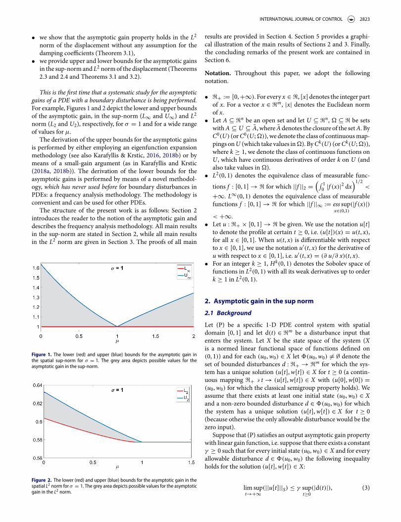
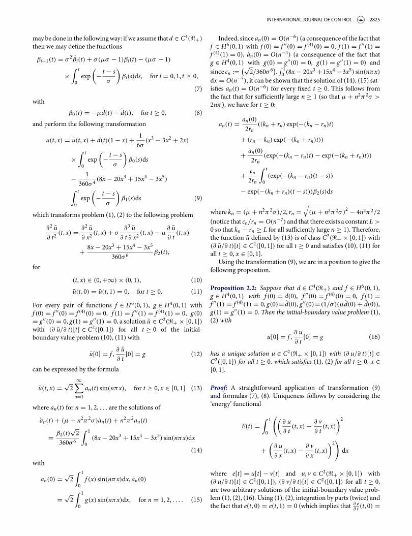
This is the !rst time that a systematic study for the asymptoticgains of a PDE with a boundary disturbance is being performed.For example, Figures 1 and 2 depict the lower and upper boundsof the asymptotic gain, in the sup-norm (L∞ and U∞) and L2norm (L2 and U2), respectively, for σ = 1 and for a wide rangeof values for µ.

The derivation of the upper bounds for the asymptotic gainsis performed by either employing an eigenfunction expansionmethodology (see also Karafyllis & Krstic, 2016, 2018b) or bymeans of a small-gain argument (as in Karafyllis and Krstic(2018a, 2018b)). The derivation of the lower bounds for theasymptotic gains is performed by means of a novel methodol-ogy, which has never used before for boundary disturbances inPDEs: a frequency analysis methodology. The methodology isconvenient and can be used for other PDEs.

The structure of the present work is as follows: Section 2introduces the reader to the notion of the asymptotic gain anddescribes the frequency analysis methodology. All main resultsin the sup-norm are stated in Section 2, while all main resultsin the L2 norm are given in Section 3. The proofs of all main

Figure 1. The lower (red) and upper (blue) bounds for the asymptotic gain inthe spatial sup-norm for σ = 1. The grey area depicts possible values for theasymptotic gain in the sup-norm.

Figure 2. The lower (red) and upper (blue) bounds for the asymptotic gain in thespatial L2 norm for σ = 1. The grey area depicts possible values for the asymptoticgain in the L2 norm.

results are provided in Section 4. Section 5 provides a graphi-cal illustration of the main results of Sections 2 and 3. Finally,the concluding remarks of the present work are contained inSection 6.

Notation. Throughout this paper, we adopt the followingnotation.

• &+ := [0,+∞). For every x ∈ &, [x] denotes the integer partof x. For a vector x ∈ &m, |x| denotes the Euclidean normof x.

• Let A ⊆ &n be an open set and let U ⊆ &n, # ⊆ & be setswithA ⊆ U ⊆ A, where Adenotes the closure of the setA. ByC0(U) (orC0(U;#)), we denote the class of continuousmap-pings onU (which take values in#). ByCk(U) (orCk(U;#)),where k ≥ 1, we denote the class of continuous functions onU, which have continuous derivatives of order k on U (andalso take values in #).

• L2(0, 1) denotes the equivalence class of measurable func-

tions f : [0, 1] → & for which ||f ||2 =(∫ 1

0 |f (x)|2 dx)1/2

<

+∞. L∞(0, 1) denotes the equivalence class of measurablefunctions f : [0, 1] → & for which ||f ||∞ := ess sup

x∈(0,1)(|f (x)|)

< +∞.• Let u : &+ × [0, 1] → & be given. We use the notation u[t]

to denote the pro!le at certain t ≥ 0, i.e. (u[t])(x) = u(t, x),for all x ∈ [0, 1]. When u(t, x) is di#erentiable with respectto x ∈ [0, 1], we use the notation u′(t, x) for the derivative ofu with respect to x ∈ [0, 1], i.e. u′(t, x) = (∂ u/∂ x)(t, x).

• For an integer k ≥ 1, Hk(0, 1) denotes the Sobolev space offunctions in L2(0, 1) with all its weak derivatives up to orderk ≥ 1 in L2(0, 1).

2. Asymptotic gain in the sup norm

2.1 Background

Let (P) be a speci!c 1-D PDE control system with spatialdomain [0, 1] and let d(t) ∈ &m be a disturbance input thatenters the system. Let X be the state space of the system (Xis a normed linear functional space of functions de!ned on(0, 1)) and for each (u0,w0) ∈ X let $(u0,w0) *= ∅ denote theset of bounded disturbances d : &+ → &m for which the sys-tem has a unique solution (u[t],w[t]) ∈ X for t ≥ 0 (a contin-uous mapping &+ ! t → (u[t],w[t]) ∈ X with (u[0],w[0]) =(u0,w0) for which the classical semigroup property holds). Weassume that there exists at least one initial state (u0,w0) ∈ Xand a non-zero bounded disturbance d ∈ $(u0,w0) for whichthe system has a unique solution (u[t],w[t]) ∈ X for t ≥ 0(because otherwise the only allowable disturbance would be thezero input).

Suppose that (P) satis!es an output asymptotic gain propertywith linear gain function, i.e. suppose that there exists a constantγ ≥ 0 such that for every initial state (u0,w0) ∈ X and for everyallowable disturbance d ∈ $(u0,w0) the following inequalityholds for the solution (u[t],w[t]) ∈ X:

lim supt→+∞

(||u[t]||S) ≤ γ supt≥0

(|d(t)|), (3)

2824 I. KARAFYLLIS ET AL.

where ||u[t]||S is the norm of a functional space S of func-tions de!ned on (0, 1). Two things should be emphasised at thispoint:

(1) Property (3) is an output asymptotic gain property. Noticethat the state may have additional components, denotedhere by w[t]. The output map is the map X ! (u,w) → u ∈S, where S is a normed linear functional space (of functionsde!ned on (0, 1)) with norm ||.||S. We assume that the mapX ! (u,w) → u ∈ S is continuous. Notice that even in thecase where the only component of the state is u[t], the out-put map is not the identity mapping when norm ||.||S doesnot coincidewith the normofX. For instance,Xmay be theH1(0, 1) space while the norm ||.||S may be the sup normor the L2 norm.

(2) Property (3) is an output asymptotic gain property withlinear gain function. The function g(supt≥0(|d(t)|)) =γ supt≥0(|d(t)|) that appears on the right hand side of (3)is linear. This feature allows us to use the name ‘d-to-uasymptotic gain in the norm of S’ for the quantity

γ‖ ‖ := sup

lim supt→+∞

(||u[t]||S)

supt≥0

(|d(t)|): (u0,w0) ∈ X,

d ∈ $(u0,w0), d *= 0

≤ γ , (4)

where (u[t],w[t])∈X denotes the solutionwith (u[0],w[0])= (u0,w0), corresponding to d ∈ $(u0,w0).

It should be noticed that γ‖ ‖, i.e. the d-to-u asymptotic gainin the norm of S de!ned by (4), is the smallest constant γ ≥ 0for which (3) holds for every initial state (u0,w0) ∈ X and forevery bounded disturbance d : &+ → &m for which the systemhas a unique solution (u[t],w[t]) ∈ X for t ≥ 0.

Remark 2.1: (a) Due to the semigroup property, the outputasymptotic gain property with linear gain function (3)holds if and only if the following inequality holds for everyinitial state (u0,w0) ∈ X and for every d ∈ $(u0,w0):

lim supt→+∞

(||u[t]||S) ≤ γ lim supt→+∞

(|d(t)|). (5)

Therefore, the d-to-u asymptotic gain in the norm of Sde!ned by (4) satis!es the following equation

γ‖ ‖ = sup

lim supt→+∞

(||u[t]||S)

lim supt→+∞

(|d(t)|): (u0,w0) ∈ X,

d ∈ $(u0,w0), lim supt→+∞

(|d(t)|) > 0

provided that there exists at least one initial state (u0,w0) ∈ Xand a disturbance d ∈ $(u0,w0)with lim sup

t→+∞(|d(t)|) > 0. If for

every (u0,w0) ∈ X the allowable disturbance set$(u0,w0) con-tains only disturbances d : &+ → &m with lim sup

t→+∞(|d(t)|) = 0,

then de!nition (4) and inequality (5) imply that γ‖ ‖ = 0.

(a) The ratio limt→+∞

(||u[t]||S)/ limt→+∞

(|d(t)|) for disturbancesd ∈ $(u0,w0) which have a limit as t → +∞ may becomputed by using the Laplace transform of the PDEin many linear PDEs. However, we emphasise that theasymptotic gain γ‖ ‖ cannot be computed by using theratio lim

t→+∞(||u[t]||S)/ lim

t→+∞(|d(t)|) for disturbances d ∈

$(u0,w0) that have a limit as t → +∞. It should benoticed that de!nition (4) involves all allowable dis-turbances (and not only those that have a limit ast → +∞) and is based on the vastly di#erent ratiolim supt→+∞

(||u[t]||S)/supt≥0

(|d(t)|).

2.2 Frequency analysis

The frequency analysis of the d-to-u asymptotic gain in thenorm of S consists of two steps.

Step 1: Let dω : &+ → &m be a parameterised family ofnon-zero inputs, with parameter ω > 0, which are periodicwith period T = 2π/ω, i.e. dω(t + 2π/ω) = dω(t) for all t ≥ 0.For each ω > 0, !nd a periodic solution (uω[t],wω[t]) ∈ X of(P) with period T = 2π/ω that corresponds to the input dω :&+ → &m.

Step 2: If Step 1 can be accomplished, then estimate the d-to-u asymptotic gain in the norm of S, by means of the followinginequality

supω>0

max

0≤t≤2π/ω(||uω[t]||S)

sup0≤t<2π/ω

(|dω(t)|)

≤ γ‖ ‖. (6)

Inequality (6) is a direct consequence of (4), the fact that(uω[t],wω[t]) ∈ X is a periodic solution of (P) with periodT = 2π/ω that corresponds to the non-zero input dω : &+ →&m and the fact that the mappings X ! (u,w) → u ∈ S, &+ !t → (u[t],w[t]) ∈ X are continuous mappings (and thereforemax

0≤t≤2π/ω(||uω[t]||S) exists for each ω > 0).

2.3 Wave equationwith Kelvin–Voigt and viscousdamping

Consider the wave equation with Kelvin–Voigt and viscousdamping (1), (2), where σ > 0, µ ≥ 0 are constants. With-out loss of generality, the tension, i.e. the coe"cient of(∂2 u/∂ x2)(t, x) in (1) has been assumed to be equal to 1; thiscan always be achieved with appropriate time scaling. For thissystem the disturbance is scalar, i.e. d : &+ → &m withm = 1.

In order to obtain an existence/uniqueness result for thewaveequation with Kelvin–Voigt and viscous damping, we !rst needto move the disturbance from the boundary to the domain andmake the boundary conditions homogeneous. However, thisprocess should be done with caution because we would also likethe non-homogeneous term that will appear in the PDE to beexpressed by a su"ciently fast convergent Fourier series. This

INTERNATIONAL JOURNAL OF CONTROL 2825

may be done in the followingway: if we assume that d ∈ C4(&+)

then we may de!ne the functions

βi+1(t) = σ 2βi(t) + σ (µσ − 1)βi(t) − (µσ − 1)

×∫ t

0exp

(− t − s

σ

)βi(s)ds, for i = 0, 1, t ≥ 0,

(7)

withβ0(t) = −µd(t) − d(t), for t ≥ 0, (8)

and perform the following transformation

u(t, x) = u(t, x) + d(t)(1 − x) + 16σ

(x3 − 3x2 + 2x)

×∫ t

0exp

(− t − s

σ

)β0(s)ds

− 1360σ 4 (8x − 20x3 + 15x4 − 3x5)

∫ t

0exp

(− t − s

σ

)β1(s)ds (9)

which transforms problem (1), (2) to the following problem

∂2 u∂ t2

(t, x) = ∂2 u∂ x2

(t, x) + σ∂3 u

∂ t ∂ x2(t, x) − µ

∂ u∂ t

(t, x)

+ 8x − 20x3 + 15x4 − 3x5

360σ 6 β2(t),

for

(t, x) ∈ (0,+∞) × (0, 1), (10)

u(t, 0) = u(t, 1) = 0, for t ≥ 0. (11)

For every pair of functions f ∈ H6(0, 1), g ∈ H4(0, 1) withf (0) = f ′′(0) = f (4)(0) = 0, f (1) = f ′′(1) = f (4)(1) = 0, g(0)= g′′(0) = 0, g(1) = g′′(1) = 0, a solution u ∈ C2(&+ × [0, 1])with (∂ u/∂ t)[t] ∈ C2([0, 1]) for all t ≥ 0 of the initial-boundary value problem (10), (11) with

u[0] = f ,∂ u∂ t

[0] = g (12)

can be expressed by the formula

u(t, x) =√2

∞∑

n=1an(t) sin(nπx), for t ≥ 0, x ∈ [0, 1] (13)

where an(t) for n = 1, 2, . . . are the solutions of

an(t) + (µ + n2π2σ )an(t) + n2π2an(t)

= β2(t)√2

360σ 6

∫ 1

0(8x − 20x3 + 15x4 − 3x5) sin(nπx)dx

(14)

with

an(0) =√2∫ 1

0f (x) sin(nπx)dx, an(0)

=√2∫ 1

0g(x) sin(nπx)dx, for n = 1, 2, . . . . (15)

Indeed, since an(0) = O(n−6) (a consequence of the fact thatf ∈ H6(0, 1) with f (0) = f ′′(0) = f (4)(0) = 0, f (1) = f ′′(1) =f (4)(1) = 0), an(0) = O(n−4) (a consequence of the fact thatg ∈ H4(0, 1) with g(0) = g′′(0) = 0, g(1) = g′′(1) = 0) andsince cn :=

(√2/360σ 6).

∫ 10 (8x − 20x3 +15x4 −3x5) sin(nπx)

dx = O(n−5), it can be shown that the solution of (14), (15) sat-is!es an(t) = O(n−6) for every !xed t ≥ 0. This follows fromthe fact that for su"ciently large n ≥ 1 (so that µ + n2π2σ >

2nπ), we have for t ≥ 0:

an(t) = an(0)2rn

((kn + rn) exp(−(kn − rn)t)

+ (rn − kn) exp(−(kn + rn)t))

+ an(0)2rn

(exp(−(kn − rn)t) − exp(−(kn + rn)t))

+ cn2rn

∫ t

0(exp(−(kn − rn)(t − s))

− exp(−(kn + rn)(t − s)))β2(s)ds

where kn = (µ + n2π2σ )/2, rn =√

(µ + n2π2σ )2 − 4n2π2/2

(notice that cn/rn = O(n−7) and that there exists a constant L >

0 so that kn − rn ≥ L for all su"ciently large n ≥ 1). Therefore,the function u de!ned by (13) is of class C2(&+ × [0, 1]) with(∂ u/∂ t)[t] ∈ C2([0, 1]) for all t ≥ 0 and satis!es (10), (11) forall t ≥ 0, x ∈ [0, 1].

Using the transformation (9), we are in a position to give thefollowing proposition.

Proposition 2.2: Suppose that d ∈ C4(&+) and f ∈ H6(0, 1),g ∈ H4(0, 1) with f (0) = d(0), f ′′(0) = f (4)(0) = 0, f (1) =f ′′(1) = f (4)(1) = 0, g(0)= d(0), g′′(0)=(1/σ )(µd(0) + d(0)),g(1) = g′′(1) = 0. Then the initial-boundary value problem (1),(2) with

u[0] = f ,∂ u∂ t

[0] = g (16)

has a unique solution u ∈ C2(&+ × [0, 1]) with (∂ u/∂ t)[t] ∈C2([0, 1]) for all t ≥ 0, which satis!es (1), (2) for all t ≥ 0, x ∈[0, 1].

Proof: A straightforward application of transformation (9)and formulas (7), (8). Uniqueness follows by considering the‘energy’ functional

E(t) =∫ 1

0

((∂ u∂ t

(t, x) − ∂ v∂ t

(t, x))2

+(

∂ u∂ x

(t, x) − ∂ v∂ x

(t, x))2)

dx

where e[t] = u[t] − v[t] and u, v ∈ C2(&+ × [0, 1]) with(∂ u/∂ t)[t] ∈ C2([0, 1]), (∂ v/∂ t)[t] ∈ C2([0, 1]) for all t ≥ 0,are two arbitrary solutions of the initial-boundary value prob-lem (1), (2), (16). Using (1), (2), integration by parts (twice) andthe fact that e(t, 0) = e(t, 1) = 0 (which implies that ∂ e

∂ t (t, 0) =

2826 I. KARAFYLLIS ET AL.

∂ e∂ t (t, 1) = 0), we obtain for all t ≥ 0:

E(t) = −2σ∫ 1

0

(∂2 e

∂ t ∂ x(t, x)

)2dx

− 2µ∫ 1

0

(∂ e∂ t

(t, x))2

dx. !

Since E(t) ≤ 0 for all t ≥ 0 and since E(0) = 0, we obtainthat E(t) = 0 for all t ≥ 0. This implies that (∂ u/∂ x)(t, x) =(∂ v/∂ x)(t, x) for all t ≥ 0, x ∈ [0, 1], which gives u ≡ v. Theproof is complete.

LetX be the linear space of all (f , g) ∈ C2([0, 1]) × C2([0, 1])for which there exists a bounded input d ∈ C2(&+) such thatthe initial-boundary value problem (1), (2), (16) has a uniquesolution u ∈ C2(&+ × [0, 1]) with (∂ u/∂ t)[t] ∈ C2([0, 1]) forall t ≥ 0. Notice that Proposition 2.2 guarantees that D ⊆ X,where

D = {(f , g) ∈ H6(0, 1) × H4(0, 1) : f ′′(0) = f (4)(0) = f (1)

= f ′′(1) = f (4)(1) = g(1) = g′′(1) = 0}.

For every (f , g) ∈ X, let $(f , g) denote the set of bounded dis-turbances d ∈ C2(&+) for which the initial-boundary valueproblem (1), (2), (16) has a unique solutionu ∈ C2(&+ × [0, 1])with (∂ u/∂ t)[t] ∈ C2([0, 1]) for all t ≥ 0. The linear space X isequipped with the norm ||(f , g)||X = ||f ||∞ + ||g||∞; thereforeit becomes clear that for every (f , g) ∈ X, d ∈ $(f , g) the map-ping &+ ! t →

(u[t], ∂ u

∂ t [t])

∈ X with(u[0], ∂ u

∂ t [0])

= (f , g) iscontinuous.

2.4 Asymptotic gain in the sup norm

We assume that the following assumption holds.

(H1) There exists a constant γ ≥ 0 such that for everybounded disturbance d ∈ C2(&+) for which (1), (2) hasa unique solution u ∈ C2(&+ × [0, 1]) with (∂ u/∂ t)[t]∈ C2([0, 1]) for all t ≥ 0, the following inequality holds:

lim supt→+∞

(||u[t]||∞) ≤ γ supt≥0

(|d(t)|). (17)

It was shown by Karafyllis and Krstic (2018a) that Assump-tion (H1) holds when 2 < 2µσ + σ 2π2. It is clear that the con-dition 2 < 2µσ + σ 2π2 implies that su"ciently large damp-ing (friction) is present in the string. When Assumption(H1) holds, we are in a position to de!ne the asymptoticgain of the displacement in the sup norm by means of theformula

γ∞ := sup

lim supt→+∞

(||u[t]||∞)

supt≥0

(|d(t)|): (f , g) ∈ X, d ∈ $(f , g), d *= 0

,

(18)

where u ∈ C2(&+ × [0, 1])with (∂ u/∂ t)[t] ∈ C2([0, 1]) for allt ≥ 0 is the solution of the initial-boundary value problem (1),(2), (16). The results by Karafyllis and Krstic (2018a) show that

when 2 < 2µσ + σ 2π2, the following inequality holds

γ∞ ≤ g(

µσ − 1σ 2

), (19)

where g(s) := inf{1/(sin(θ)

(1 −

√p(s, θ)

)2) : 0 < θ <(π −

√|s| − s

)/2}and p(s, θ) := |s|/(s + (π − 2θ)2).

Our !rst main result in the present work concerning the supnorm is a sharper result than the result given by Karafyllis andKrstic (2018a). Its proof is provided in Section 4.

Theorem 2.3: Consider the wave equation with Kelvin–Voigtand viscous damping (1), (2), where σ > 0, µ ≥ 0 are con-stants with 2 < 2µσ + σ 2π2. Then Assumption (H1) holds andinequality (19) holds with g(s) := inf

{1/(sin(θ)(1 − p(s, θ))) :

0 < θ < π −√

|s| − s}and p(s, θ) := |s|/(s + (π − θ)2).

Our second main result in the present work concerning thesup norm is given below and it is proved by means of the fre-quency analysis procedure that was described above. Its proof isprovided in Section 4.

Theorem 2.4: Consider the wave equation with Kelvin–Voigtand viscous damping (1), (2), where σ > 0, µ ≥ 0 are constants.Suppose that Assumption (H1) holds. De!ne for each ω > 0:

r :=ω

√(µσ − 1)2ω2 + (µ + σω2)2

1 + σ 2ω2 , (20)

a :=√r cos(θ/2)

b :=√r sin(θ/2) (21)

where θ ∈ (0,π) is the unique angle that satis!es the equations

cos(θ) = (µσ − 1)ω2

(1 + σ 2ω2)r, sin(θ) = (µ + σω2)ω

(1 + σ 2ω2)r. (22)

Then the following inequality holds:

γ∞ ≥ supω>0

√√√√ maxx∈[0,1]

(cosh(2ax) − cos(2bx))

cosh(2a) − cos(2b)

. (23)

Noticing that the right hand side of (23) is always greateror equal to 1, Theorem 2.3 allows us to obtain the followingcorollary for the sup norm.

Corollary 2.5: Consider the wave equation with Kelvin–Voigtand viscous damping (1), (2), where σ > 0, µ ≥ 0 are constants.Suppose that µσ = 1. Then γ∞ = 1.

3. Asymptotic gain in the L2 norm

3.1 Existence of asymptotic gain in the L2 norm

It is not clear whether Assumption (H1) holds for all σ > 0,µ ≥ 0 for the wave equation with Kelvin–Voigt and viscousdamping. However, the analogue of Assumption (H1) for the L2

INTERNATIONAL JOURNAL OF CONTROL 2827

norm holds for all σ > 0, µ ≥ 0. This is a consequence of thefollowing theorem.

Theorem 3.1: Consider the wave equation with Kelvin–Voigtand viscous damping (1), (2), where σ > 0, µ ≥ 0 are constants.There exists a constant γ ≥ 0 such that for every bounded dis-turbance d ∈ C2(&+) for which (1), (2) has a unique solutionu ∈ C2(&+ × [0, 1]) with (∂ u/∂ t)[t] ∈ C2([0, 1]) for all t ≥ 0,the following inequality holds:

lim supt→+∞

(||u[t]||2) ≤ γ supt≥0

(|d(t)|). (24)

Moreover, the constant γ ≥ 0 satis!es the inequality

γ ≤ G(µ, σ ), (25)

where

G(µ, σ ) :=

1√3

if µσ ≥ 1

1π

√

2∞∑n=1

n−2A2n if 0 ≤ µσ < 1

(26)

and

An = 1 + 2√1 − µσ

(2βn

√1 − µσ

σ (µ + n2π2σ )(1 + βn) − 2βn

)βn

,

βn : = µ + n2π2σ√

(µ + n2π2σ )2 − 4n2π2

,

if µ + n2π2σ > 2nπ ≥ 2σ−1, (27)

An = 1, if nπσ < 1 and µ + n2π2σ ≥ 2nπ , (28)

An = 1 + 2√1 − µσ exp

(−1 − 1√

1 − µσ

),

if nπσ = 1 +√1 − µσ , (29)

An = 1 + 2√1 − σµ

exp(

(µ+n2π2σ )√4n2π2−(µ+n2π2σ )

2

arccos(2−σµ−n2π2σ 2

2√1−σµ

))

exp(

(µ+n2π2σ )π√4n2π2−(µ+n2π2σ )

2

)− 1

,

if µ + n2π2σ < 2nπ . (30)

The proof of Theorem 3.1 can be found in the followingsection. A direct consequence of Theorem 3.1 is the fact thatfor every σ > 0, µ ≥ 0, we can de!ne the asymptotic gain ofthe displacement in the L2 norm for the wave equation withKelvin–Voigt and viscous damping in the following way:

γ2 := sup

lim supt→+∞

(||u[t]||2)

supt≥0

(|d(t)|): (f , g) ∈ X, d∈$(f , g), d *= 0

,

(31)where u ∈ C2(&+ × [0, 1])with (∂ u/∂ t)[t] ∈ C2([0, 1]) for allt ≥ 0 is the solution of the initial-boundary value problem

(1), (2), (16). Moreover, it follows from Theorem 3.1 that thefollowing inequality holds:

γ2 ≤ G(µ, σ ), (32)

where the function G(µ, σ ) is de!ned by (26). Finally, ifAssumption (H1) holds then the following inequality is adirect consequence of the fact that ||u||2 ≤ ||u||∞ for all u ∈C0([0, 1]):

γ2 ≤ γ∞. (33)

3.2 Lower bound of asymptotic gain in the L2 norm

Our second main result in the present work concerning theL2 norm is given below and it is proved by means of the fre-quency analysis procedure that was described above. Its proof isprovided in Section 4.

Theorem 3.2: Consider the wave equation with Kelvin–Voigtand viscous damping (1), (2), where σ > 0, µ ≥ 0 are constants.De!ne r, a, b by means of (20), (21) for each ω > 0, where θ ∈(0,π) is the unique angle that satis!es equations (22). Then thefollowing inequality holds:

γ2 ≥ supω>0

(Q(ω)), (34)

where Q(ω) :=√p +

√M with

M :=1

4(cosh(2a) − cos(2b))2+

sinh2(2a) + sin2(2b)−4(b sin(2b)cosh(2a)+a sinh(2a)cos(2b))16(a2 + b2)(cosh(2a)

−cos(2b))2

(35)

p = b sinh(2a) − asin(2b)4ab(cosh(2a) − cos(2b))

. (36)

Combining Theorem3.1 andTheorem3.2, we get the follow-ing corollary, which is proved in the following section.

Corollary 3.3: Consider the wave equation with Kelvin–Voigtand viscous damping (1), (2), where σ > 0, µ ≥ 0 are constants.Suppose that µσ ≥ 1. Then γ2 = 1/

√3.

It is clear that the condition µσ ≥ 1 implies the vibratingstring becomes overdamped when µσ ≥ 1 and the boundaryforcing cannot produce large (in the L2 norm) oscillations inthe string.

4. Proofs of main results

Proof of Theorem 2.3: The fact that Assumption (H1) holdswhen 2 < 2µσ + σ 2π2 is a direct consequence of Theorem2.2 by Karafyllis and Krstic (2018a). We next notice that everysolution u ∈ C2(&+ × [0, 1]) with (∂ u/∂ t)[t] ∈ C2([0, 1]) for

2828 I. KARAFYLLIS ET AL.

all t ≥ 0, of (1), (2) is a solution of the system of the integro-di#erential equation

∂ u∂ t

(t, x) = σ∂2 u∂ x2

(t, x) − µσ − 1σ

u(t, x)

+ µσ − 1σ 2

∫ t

0exp

(− t − s

σ

)u(s, x)ds

+ exp(

− tσ

)(∂ u∂ t

(0, x) − σ∂2 u∂ x2

(0, x)

+ µσ − 1σ

u(0, x))

(37)

Let θ ∈ (0,π), ϕ ∈ [0,π − θ) be a pair of angles with|µσ − 1| + 1 − µσ < σ 2ϕ2 (such a pair of angles exists dueto the fact that 2 < 2µσ + σ 2π2). De!ne the positive func-tion η(x) := sin(θ + ϕx) for x ∈ [0, 1] and the norm ||u||∞,η :=max0≤x≤1

(|u(x)|/η(x)) . Notice that Assumptions (H1), (H2), (H3),

(H4) by Karafyllis and Krstic (2018a) hold for the PDE problem

∂ u∂ t

(t, x) = ∂2 u∂ x2

(t, x) − µσ − 1σ

u(t, x) + f (t, x)

with u(t, 0) − d(t) = u(t, 1) = 0. Applying Corollary 4.3 byKarafyllis and Krstic (2018a) to (37) with

f (t, x) = µσ − 1σ 2

∫ t

0exp

(− t − s

σ

)u(s, x)ds

+ exp(

− tσ

)(∂ u∂ t

(0, x) − σ∂2 u∂ x2

(0, x)

+ µσ − 1σ

u(0, x))

and using the semigroup property and the fact that lim supt→+∞

(||f [t]||∞,η) ≤ |µσ−1|σ sup

t→+∞(||u[t]||∞,η), we get

lim supt→+∞

(||u[t]||∞,η) ≤ 1sin(θ)

lim supt→+∞

(|d(t)|) + |µσ − 1|µσ − 1

+σ 2ϕ2 lim supt→+∞

(||u[t]||∞,η)

It follows from the above inequality and the fact that ||u||∞ ≤||u||∞,η for all u ∈ C0([0, 1]) that γ∞ ≤ 1/((1 − |s|/(s + ϕ2))sin(θ)) for all θ ∈ (0,π), ϕ ∈ [0,π − θ) with |s| − s < ϕ2 ands := (µσ − 1)/σ 2. Therefore, for every θ ∈ (0,π) with θ <

π −√

|s| − s, it holds that γ∞ ≤ 1/((1 − |s|/(s + (π − θ)2))sin(θ)). Thus, inequality (19) holds with g(s) := inf {1/(sin(θ)

(1 − p(s, θ))) : 0 < θ < π −√

|s| − s}

and p(s, θ) := |s|/(s + (π − θ)2). The proof is complete.

Proof of Theorem 2.4: We apply the frequency analysismethodology for the parameterised family of inputs dω(t) =sin(ωt) with parameter ω > 0. A periodic solution uω[t] of (1),(2) that corresponds to the input dω(t) = sin(ωt) is given by the

formula

uω(t, x) = sin(ωt)h(x) + cos(ωt)g(x), for t ≥ 0, x ∈ [0, 1](38)

where h,g are solutions of the boundary-value problem

σωg′′(x) − µωg(x) − ω2h(x) − h′′(x) = 0ω2g(x) + g′′(x) + σωh′′(x) − µωh(x) = 0, (39)

h(0) = 1, h(1) = g(0) = g(1) = 0. (40)

It can be veri!ed that the functions

h(x) =

(cosh(a(2 − x)) − cos(2b) cosh(ax)) cos(bx)− sin(2b) sin(bx) cosh(ax)

cosh(2a) − cos(2b)

g(x) =

sin(2b) cos(bx) sinh(ax) − (sinh(a(2 − x))+cos(2b) sinh(ax)) sin(bx)

cosh(2a) − cos(2b)(41)

where a,b are de!ned by (21), are solutions of the boundary-value problem (39), (40). Using (6) and (38), we obtain theinequality

supω>0

(max

0≤t≤2π/ω

(max0≤x≤1

(|sin(ωt)h(x) + cos(ωt)g(x)|)))

≤ γ∞.

(42)Since

max0≤t≤2π/ω

(max0≤x≤1

(|sin(ωt)h(x) + cos(ωt)g(x)|))

= max0≤x≤1

(max

0≤t≤2π/ω(|sin(ωt)h(x) + cos(ωt)g(x)|)

)

= max0≤x≤1

(√h2(x) + g2(x)

)(43)

and since (41) implies that

h2(x) + g2(x) = cosh(2a(1 − x)) − cos(2b(1 − x))cosh(2a) − cos(2b)

,

for x ∈ [0, 1], (44)

we obtain from (42), (43) and (44) the desired inequality (23).The proof is complete.

Proof of Theorem 3.1: It su"ces to show that there existsa constant γ ≥ 0 such that for every bounded disturbanced ∈ C2(&+) for which (1), (2) has a unique solution u ∈C2(&+ × [0, 1])with (∂ u/∂ t)[t] ∈ C2([0, 1]) for all t ≥ 0, withthe following property:

For every ε > 0 there exists T > 0 such that ||u[t]||2 ≤γ sup

s≥0(|d(s)|) + ε for all t ≥ T.

Let an arbitrary bounded disturbance d ∈ C2(&+) for which(1), (2) has a unique solution u ∈ C2(&+ × [0, 1]) with

INTERNATIONAL JOURNAL OF CONTROL 2829

(∂ u/∂ t)[t] ∈ C2([0, 1]) for all t ≥ 0. De!ne:

yn(t) =√2∫ 1

0u(t, x) sin(nπx)dx, for n = 1, 2, . . . . (45)

De!nition (45) in conjunction with (1), (2) implies that the fol-lowing di#erential equations hold for all t ≥ 0 and n = 1, 2, . . .:

yn(t) + (µ + n2π2σ )yn(t) + n2π2yn(t)

= nπ√2(σ d(t) + d(t)) (46)

When µ + n2π2σ > 2nπ then we may de!ne

kn := µ + n2π2σ

2, rn :=

√(µ + n2π2σ )

2 − 4n2π2

2(47)

and express the solution of (46) by the following formula:

yn(t) = exp(−(kn − rn)t)2rn

((kn + rn − (kn − rn)

× exp(−2rnt))yn(0)+yn(0)(1 − exp(−2rnt)))

− nπσ

rn√2exp(−(kn − rn)t)(1 − exp(−2rnt))d(0)

+ gn(t), (48)

gn(t) : =nπrn

√2

∫ t

0((σkn + σ rn − 1) exp(−(kn + rn)(t − τ ))

+ (1 + σ rn − σkn) exp(−(kn − rn)(t − τ ))) d(τ ) dτ .(49)

When nπσ = 1 ±√1 − µσ (or equivalently when µ + n2π2

σ = 2nπ) then the solution of (46) is given by the followingformulas:

yn(t) = (1 + knt)yn(0) exp(−knt) + yn(0)t exp(−knt)

− nπσ√2t exp(−knt)d(0) + gn(t), (50)

gn(t) = nπ√2∫ t

0(σ + (1 − σkn)(t − s))

exp(−kn(t − s)) d(s) ds. (51)

When µ + n2π2σ < 2nπ then we may de!ne:

ωn :=

√4n2π2 − (µ + n2π2σ )

2

2(52)

and in this case the solution of (46) is given by the followingformulas:

yn(t) = yn(0)(knωn

sin(ωnt) + cos(ωnt))exp(−knt)

+ yn(0)ωn

sin(ωnt) exp(−knt)

− nπσ√2

ωnsin(ωnt) exp(−knt)d(0) + gn(t), (53)

gn(t) = nπ√2

ωn

∫ t

0(σωn cos(ωn(t − s))

+ (1 − σkn) sin(ωn(t − s))) exp(−kn(t − s)) d(s) ds.(54)

We next show that for every θ > 0 there exists T > 0 thatdepends only on the initial conditions, such that for all t ≥ Tit holds that:

|yn(t) − gn(t)| ≤ θ

nfor all t ≥ T, n = 1, 2, . . . (55)

De!nitions (47) imply that there exist positive constantsδ, β , c > 0 so that the following inequalities hold for all n ≥ 1with µ + n2π2σ > 2nπ :

δ ≥ 2n2π2

µ+n2π2σ≥ kn − rn ≥ n2π2

µ+n2π2σ≥ β

rn ≥ cn2π2(56)

It follows from (48) and (56) that the following estimate holdsfor all t ≥ 0 and n ≥ 1 with µ + n2π2σ > 2nπ :

|yn(t) − gn(t)| ≤ exp(−βt)2rn

((kn + rn)|yn(0)| + |yn(0)|)

+ σ

cnπ√2exp(−βt)|d(0)|. (57)

De!nition (45) and (2) imply that yn(t) =√2d(t)/(nπ) +(√

2/(nπ)) ∫ 1

0 u′(t, x) cos(nπx)dx. Therefore, we get:

|yn(t)| ≤√2|d(t)|nπ

+ 1nπ

||u′[t]||2, for all t ≥ 0, n = 1, 2, . . .(58)

Similarly, de!nition (45) implies that:

|yn(t)| ≤∥∥∥∥∂ u∂ t

[t]∥∥∥∥2, for all t ≥ 0 and n ≥ 1. (59)

Using (2), (56), (57), (58) and (59), we obtain for all t ≥ 0 andn ≥ 1 with µ + n2π2σ > 2nπ :

|yn(t) − gn(t)|

≤ exp(−βt)2rn

((δ + 2rn)

1nπ

(√2|u(0, 0)| + ||u′[0]||2

)

+∥∥∥∥∂ u∂ t

[0]∥∥∥∥2

)+ σ

cnπ√2exp(−βt)|u(0, 0)|. (60)

It follows from (56) and (60) that the following inequalityholds for all t ≥ 0 and n ≥ 1 with µ + n2π2σ > 2nπ :

|yn(t) − gn(t)|

≤ exp(−βt)2nπ

((2 + δ

cπ2

)(√2|u(0, 0)| + ||u′[0]||2

)

+ 1cπ

∥∥∥∥∂ u∂ t

[0]∥∥∥∥2+ σ

c√2|u(0, 0)|

)(61)

If µ + n2π2σ > 2nπ holds for all integers n ≥ 1 then (55) is adirect consequence of (61). We next consider the case that thereexist integers n ≥ 1 for which µ + n2π2σ ≤ 2nπ .

2830 I. KARAFYLLIS ET AL.

Let N ≥ 1 be the integer de!ned in the following way: N =1 if µσ > 1 and N =

[(1 +

√1 − µσ

)/(σπ)

]+ 1 if µσ ≤ 1.

Notice that µ + n2π2σ > 2nπ for all n ≥ N. Without loss ofgenerality, we may assume that the positive constant β > 0 forwhich (56) holds, also satis!es the inequality (µ + π2σ )/2 > β .It then follows from (50), (53), (58), (59) and (2) that thereexists a constant G > 0 (depending only on the initial condi-tions) such that the following inequality holds for all t ≥ 0 andn = 1, . . . ,N − 1 with µ + n2π2σ ≤ 2nπ :

|yn(t) − gn(t)| ≤ G exp(−βt).

The above inequality implies that

|yn(t) − gn(t)| ≤ GN − 1n

exp(−βt). (62)

Therefore, if there exist integers n ≥ 1 for which µ + n2π2σ ≤2nπ , then (55) is a direct consequence of (61) and (62). Thus,we have shown that (55) holds.

For all n ≥ 1 with µ + n2π2σ > 2nπ , de!nitions (47), (49)imply the following estimates for all t ≥ 0:

|gn(t)| ≤ nπrn

√2||d||∞

∫ t

0|(σkn + σ rn − 1) exp(−(kn + rn)

× (t − τ )) + (1 + σ rn − σkn)

× exp(−(kn − rn)(t − τ ))|dτ

≤ nπrn

√2||d||∞

(1

kn − rn− 1

kn + rn

)

if µσ ≥ 1 or nπσ ≤ 1(equivalently if σ (kn − rn) ≤ 1) (63)

|gn(t)| ≤ nπrn

√2||d||∞

∫ t

0|(σkn + σ rn − 1) exp(−(kn + rn)

× (t − τ )) + (1 + σ rn − σkn)

× exp(−(kn − rn)(t − τ ))|dτ

≤ nπrn

√2||d||∞

(1

kn − rn− 1

kn + rn

)

×

1 + 2(

σkn − σ rn − 1σkn + σ rn − 1

) kn2rn

√(σkn + σ rn − 1)(σkn − σ rn − 1)

if µσ < 1 and nπσ > 1(equivalently if σ (kn − rn) > 1),(64)

where ||d||∞ := sups≥0(|d(s)|). Notice that µσ ≥ 1 (whichimplies µ + n2π2σ ≥ 2nπ for all n ≥ 1), de!nitions (47), (51)and estimate (63) give:

|gn(t)| ≤√2

nπ||d||∞, for all n ≥ 1 and t ≥ 0. (65)

Using (63), (64), (51), (54), (47), (52) and de!nitions (27),(28), (29), (30), we obtain the following estimates for the case

µσ < 1:

|gn(t)| ≤√2

nπAn||d||∞, for all n ≥ 1 and t ≥ 0. (66)

We are ready to !nish the proof. Let arbitrary ε > 0 be given.Since limn→+∞(An) = 1 (a consequence of de!nition (27)), itfollows that the sequence {An}∞n=1 is bounded. Let A be an upperbound for the sequence {An}∞n=1. Pick θ > 0 su"ciently smallso that θ2(π2/6) + θ

(π

√2/3

)||d||∞A ≤ ε2. Then there exists

T > 0 so that (55) holds. Using the triangle inequality, we obtainfrom (55) for all n ≥ 1 and t ≥ T:

|yn(t)|2 ≤ θ2

n2+ |gn(t)|2 + 2θ

n|gn(t)|. (67)

De!nition (45) and the fact that the set of functions {√2 sin

(nπx) : n = 1, 2, . . .} is an orthonormal basis of L2(0, 1) impliesthat Parseval’s identity holds, i.e. ||u[t]||22 =

∑∞n=1 y2n(t). If

µσ < 1 then we get from (66), (67) for all t ≥ T:

||u[t]||22 ≤ θ2∞∑

n=1n−2 + 2

π2 ||d||2∞∞∑

n=1n−2A2

n

+ 2√2

πθ ||d||∞

∞∑

n=1n−2An. (68)

Using (68) and the fact∑∞

n=1 n−2 = π2/6, we get for all t ≥ T:

||u[t]||22 ≤ θ2π2

6+ (G(µ, σ ))2||d||2∞ + π

√2

3θ ||d||∞A, (69)

where A is the upper bound for the sequence {An}∞n=1. It followsfrom (69) and the fact that θ2(π2/6) + θ

(π

√2/3

)||d||∞A ≤

ε2 that ||u[t]||2 ≤ G(µ, σ )||d||∞ + ε for all t ≥ T.The analysis is similar for the caseµσ ≥ 1 (simply setAn ≡ 1

in the above analysis).The proof is complete.

Proof of Theorem 3.2: We apply the frequency analysismethodology for the parameterised family of inputs dω(t) =sin(ωt) with parameter ω > 0. A periodic solution uω[t] of (1),(2) that corresponds to the input dω(t) = sin(ωt) is given by(38), where h, g are given by (41). Using (38), we get for all t ≥ 0:

||u[t]||22 = p + q1 cos(2ωt) + q2 sin(2ωt), (70)

where

p : = 12

∫ 1

0(h2(x) + g2(x)) dx, (71)

q1 : =12

∫ 1

0(g2(x) − h2(x)) dx, (72)

q2 : =∫ 1

0h(x)g(x) dx. (73)

INTERNATIONAL JOURNAL OF CONTROL 2831

Using (41), (44), (71), (72), (73), we obtain (36) as well as thefollowing formulas:

q1 = cosh(2a)cos(2b) − 12(cosh(2a) − cos(2b))2

+ b sin(2b) − a sinh(2a)4(a2 + b2)(cosh(2a) − cos(2b))

(74)

q2 = sinh(2a)sin(2b)2(cosh(2a) − cos(2b))2

− asin(2b) + b sinh(2a)4(a2 + b2)(cosh(2a) − cos(2b))

(75)

Equation (70) implies that

max{||u[t]||22 : 0 ≤ t ≤ 2π

ω

}= p +

√q21 + q22, (76)

Equation (76) combined with (74), (75) and (6) gives (34) withQ(ω) :=

√p +

√M andM given by (35). The proof is complete.

Proof of Corollary 3.3: It su"ces to show that limω→0+(Q(ω))

= 1/√3, where Q(ω) :=

√p +

√M with p,M de!ned by

(35), (36). Indeed, de!nitions (35), (36) imply that p → 1/6and M → 1/36 as (a, b) → (0, 0). Moreover, de!nitions (20),(21) imply that a → 0 and b → 0 as ω → 0+. The proof iscomplete.

5. Graphical illustration of the theorem statements

This section is devoted to the graphical illustration of the theo-rems’ statements for the upper and lower bounds of the asymp-totic gains. To this purpose, we de!ne:

U∞ : = g(

µσ − 1σ 2

),

for σ > 0,µ ≥ 0 with 2 < 2µσ + σ 2π2, (77)

where g(s) := inf{1/(sin(θ)(1 − p(s, θ))) : 0 < θ < π−√

|s| − s}and p(s, θ) := |s|/(s + (π − θ)2),

L∞ : = supω>0

(A(ω)), (78)

A(ω) : =

√√√√ maxx∈[0,1]

(cosh(2ax) − cos(2bx))

cosh(2a) − cos(2b), (79)

and a, b are being de!ned by (21),

L2 := supω>0

(Q(ω)), (80)

where

Q(ω) :=√p +

√M, (81)

and p,M are being de!ned by (35), (36) and

U2 := G(µ, σ ), (82)

Figure 3. The lower (red) and upper (blue) bounds for the asymptotic gain in thesup norm forσ = 0.5. The grey area depicts possible values for the asymptotic gainin the sup norm.

Figure 4. Bode-like plot of ln(A(ω)) for σ = 0.0001.

where G(µ, σ ) is de!ned by (26). Notice that the results of theprevious sections guarantee that

γ∞ ≤ U∞, for all σ > 0,

µ ≥ 0 for which Assumption (H1) holds, (83)

L∞ ≤ γ∞, for all σ > 0,

µ ≥ 0 for which Assumption (H1) holds, (84)

L2 ≤ γ2 ≤ U2, for all σ > 0,µ ≥ 0. (85)

Figures 1 and 3 depict the lower and upper bounds of theasymptotic gain in the sup norm for σ = 1 and σ = 0.5, respec-tively, and for a wide range of values for µ. Figures 4–6 areBode-like plots for the logarithm of A(ω) de!ned by (79) forσ = 0.0001, σ = 0.001 and σ = 0.01, respectively, and for fourdi#erent values of µ. These plots indicate that for small σ andµ, A(ω) presents ‘spikes’ at frequencies which di#er by π . Onthe other hand, for su"ciently large σ and µ, A(ω) identicallyequal to 1.

Figures 2 and 7 depict the lower and upper bounds of theasymptotic gain in the L2 norm, for σ = 1 and σ = 0.5, respec-tively, and for a wide range of µ values. Notice that for µσ ≥1, we get L2 = U2 = 1/

√3. Comparing Figures 2 and 7 with

Figures 1 and 3, we conclude that the asymptotic gain in the L2norm is estimated much more accurately than the asymptoticgain in the sup norm.

Figures 8–11 are Bode-like plots for the logarithm of Q(ω)

de!ned by (81) for σ = 0.0001, σ = 0.001, σ = 0.01 andσ = 0.5, respectively, and for four di#erent values of µ. As inthe sup norm, these plots indicate that for small σ and µ, Q(ω)

2832 I. KARAFYLLIS ET AL.

Figure 5. Bode-like plot of ln(A(ω)) for σ = 0.001.

Figure 6. Bode-like plot of ln(A(ω)) for σ = 0.01.

Figure 7. The lower (red) and upper (blue) bounds for the asymptotic gain in theL2 norm for σ = 0.5. The grey area depicts possible values for the asymptotic gainin the L2 norm.

Figure 8. Bode-like plot of ln(Q(ω)) for σ = 0.0001.

presents ‘spikes’ at frequencies which di#er by π . These are‘dangerous’ frequencies: the amplitude of the oscillation of theboundary of a string becomes magni!ed in its domain.

Figure 9. Bode-like plot of ln(Q(ω)) for σ = 0.001.

Figure 10. Bode-like plot of ln(Q(ω)) for σ = 0.01.

Figure 11. Bode-like plot of ln(Q(ω)) for σ = 0.5.

6. Concluding remarks

We have provided estimates for the asymptotic gains of the dis-placement of a vibrating string with external forcing. By consid-ering an external boundary disturbance for the wave equationwithKelvin–Voigt and viscous damping, we have shown that theasymptotic gain property holds in the spatial L2 norm of the dis-placementwithout any assumption for the damping coe"cients.We have also provided upper and lower bounds for the asymp-totic gains in the spatial sup-norm and the spatial L2 norm ofthe displacement.

The present work provided estimates of the asymptotic gainsof the displacement of a vibrating string with external forcingwithout any uniformity with respect to the disturbances (see thenotion of the uniform asymptotic gain property by (Sontag &Wang, 1996)). It should be noticed that the present paper stud-ied output asymptotic gain properties and not state asymptotic

INTERNATIONAL JOURNAL OF CONTROL 2833

gain properties and that uniform asymptotic gains have beende!ned only for the case where the output coincides with thestate. One can think of many di#erent extensions of the uni-form asymptotic gain property to the case of a general outputmap. In any case, a slight modi!cation of the proof of Theorem3.1 shows that the following property holds:

For every ε > 0, R > 0 there exists T = T(ε,R) > 0such that for every

(u[0], ∂ u

∂ t [0])

∈ X with ||u[0]||∞ +||u′[0]||2 +

∣∣| ∂ u∂ t [0]

∣∣ |2 ≤ R the inequality ||u[t]||2 ≤ (ε +G(µ, σ )) sup

s≥0(|d(s)|) + ε holds for all t ≥ T and d ∈

$(u[0], ∂ u

∂ t [0]).

where G(µ, σ ) is the function de!ned by (26). The above prop-erty guarantees some uniformity with respect to the allowabledisturbances.

As noted in the introduction, this is the !rst systematic studyof the asymptotic gains for a PDE with a boundary disturbance.Although here we studied the wave equation with Kelvin–Voigtand viscous damping, it is expected that similar studies will beperformed for many other important PDEs.

Disclosure statementNo potential con$ict of interest was reported by the author(s).

ReferencesAngeli, D., Ingalls, B., Sontag, E. D., & Wang, Y. (2004). Separa-

tion principles for input-output and integral-input to state stabil-ity. SIAM Journal on Control and Optimization, 43(1), 256–276.https://doi.org/10.1137/S0363012902419047

Chen, S., Liu, K., & Liu, Z. (1998). Spectrum and stability for elastic systemswith global or local Kelvin-Voigt damping. SIAM Journal on AppliedMathematics, 59(1), 651–668. https://doi.org/10.1137/S0036139996301283

Coron, J. M., Praly, L., & Teel, A. (1995). Feedback stabilization of non-linear systems: Su"cient conditions and Lyapunov and input-outputtechniques. In Alberto Isidori (Ed.), Trends in control (pp. 293–348).Springer-Verlag.

Gerbi, S., & Said-Houari, B. (2012). Existence and exponential stability of adamped wave equation with dynamic boundary conditions and a delayterm. Applied Mathematics and Computation, 218(24), 11900–11910.https://doi.org/10.1016/j.amc.2012.05.055

Guenther, R. B., & Lee, J. W. (1996). Partial di"erential equations of mathe-matical physics and integral equations. Dover.

Guo, B.-Z., Wang, J.-M., & Zhang, G.-D. (2010). Spectral analysis of a waveequation with Kelvin-Voigt damping. Zeitschrift für Angewandte Math-ematik und Mechanik, 90(4), 323–342. https://doi.org/10.1002/zamm.200900275

Karafyllis, I., & Jiang, Z.-P. (2011). Stability and stabilization of nonlinearsystems. Springer-Verlag London. (Series: Communications andControlEngineering).

Karafyllis, I., & Krstic, M. (2016). ISS with respect to boundary distur-bances for 1-Dparabolic PDEs. IEEETransactions onAutomatic Control,61(12), 3712–3724. https://doi.org/10.1109/TAC.2016.2519762

Karafyllis, I., & Krstic, M. (2017). Predictor feedback for delay systems:Implementations and approximations. Birkhäuser. (Series: Mathematics,Systems & Control: Foundations & Applications).

Karafyllis, I., & Krstic, M. (2018a). Small-gain stability analysis of cer-tain hyperbolic-parabolic PDE loops. Systems and Control Letters, 118,52–61. https://doi.org/10.1016/j.sysconle.2018.05.012

Karafyllis, I., & Krstic, M. (2018b). Input-to-state stability for PDEs.Springer-Verlag. (Series: Communications and Control Engineering).

Krstic, M., & Smyshlyaev, A. (2008). Boundary control of PDEs: A course onbackstepping designs. SIAM.

Liu, K., & Rao, B. (2006). Exponential stability for the wave equations withlocal Kelvin–Voigt damping.Zeitschrift fürAngewandteMathematik undPhysik, 57(3), 419–432. https://doi.org/10.1007/s00033-005-0029-2

Mironchenko, A. (2016). Local input-to-state stability: Characteriza-tions and counterexamples. Systems & Control Letters, 87, 23–28.https://doi.org/10.1016/j.sysconle.2015.10.014

Mironchenko, A., & Wirth, F. (2018). Characterizations of input-to-statestability for in!nite-dimensional systems. IEEE Transactions on Auto-matic Control, 63(6), 1692–1707. https://doi.org/10.1109/TAC.2017.2756341

Pellicer, M. (2008). Large time dynamics of a nonlinear spring-mass-damper model. Nonlinear Analysis: Theory, Methods & Applications,69(9), 3110–3127. https://doi.org/10.1016/j.na.2007.09.005

Pellicer, M., & Sola-Morales, J. (2004). Analysis of a viscoelastic spring-mass model. Journal of Mathematical Analysis and Applications, 294(2),687–698. https://doi.org/10.1016/j.jmaa.2004.03.008

Roman, C., Bresch-Pietri, D., Prieur, C., & Sename, O. (2016a, July 6–8).Robustness of an adaptive output feedback for an anti-damped boundarywave PDE in presence of in-domain viscous damping. Proceedings of theAmerican control Conference, Boston, MA, USA.

Roman, C., Bresch-Pietri, D., Cerpa, E., Prieur, C., & Sename, O. (2016b,December 12–14). Backstepping observer based-control for an anti-damped boundary wave PDE in presence of in-domain viscous damping.Proceedings of the 55th IEEE Conference on Decision and control (pp.549–554). Las Vegas, NV, USA.

Roman, C., Bresch-Pietri, D., Cerpa, E., Prieur, C., & Sename, O. (2018).Backstepping control of a wave PDE with unstable source termsand dynamic boundary. IEEE Control Systems Letters, 2(3), 459–464.https://doi.org/10.1109/LCSYS.2018.2841898

Siranosian, A., Krstic, M., Smyshlyaev, A., & Bement, M. (2009). Motionplanning and tracking for tip displacement and de$ection angle for$exible beams. Journal of Dynamic Systems, Measurement, and Control,131(3). https://doi.org/10.1115/1.3072152

Sontag, E. D., & Wang, Y. (1996). New characterizations of input-to-statestability. IEEE Transactions on Automatic Control, 41(9), 1283–1294.https://doi.org/10.1109/9.536498

Zhang, Q. (2010). Exponential stability of an elastic string with localKelvin–Voigt damping. Zeitschrift für Angewandte Mathematik undPhysik, 61(6), 1009–1015. https://doi.org/10.1007/s00033-010-0064-5