BOUNDING THE NUMBER OF GRAPHS CONTAINING

VERY LONG INDUCED PATHS

by

Steven Kay Butler

A thesis submitted to the faculty of

Brigham Young University

in partial fulfillment of the requirements for the degree of

Master of Science

Department of Mathematics

Brigham Young University

April 2003

BRIGHAM YOUNG UNIVERSITY

GRADUATE COMMITTEE APPROVAL

of a thesis submitted by

Steven Kay Butler

This thesis has been read by each member of the following graduate committee andby majority vote has been found to be satisfactory.

Date Wayne W. Barrett, Chair

Date James W. Cannon

Date Rodney W. Forcade

BRIGHAM YOUNG UNIVERSITY

As chair of the candidate’s graduate committee, I have read the thesis of StevenKay Butler in its final form and have found that (1) its format, citations, andbibliographical style are consistent and acceptable and fulfill university anddepartment style requirements; (2) its illustrative materials including figures, tables,and charts are in place; and (3) the final manuscript is satisfactory to the graduatecommittee and is ready for submission to the university library.

Date Wayne W. BarrettChair, Graduate Committee

Accepted for the DepartmentTyler J. JarvisGraduate Coordinator

Accepted for the CollegeG. Rex Bryce, Associate DeanCollege of Physical and Mathematical Sciences

ABSTRACT

BOUNDING THE NUMBER OF GRAPHS CONTAINING

VERY LONG INDUCED PATHS

Steven Kay Butler

Department of Mathematics

Master of Science

Induced graphs are used to describe the structure of a graph, one such type

of induced graph that has been studied are long paths.

In this thesis we show a way to represent such graphs in terms of an array

with two colors and a labeled graph. Using this representation and the techniques of

Polya counting we will then be able to get upper and lower bounds for graphs

containing a long path as an induced subgraph.

In particular, if we let P(n, k) be the number of graphs on n + k vertices

which contains Pn, a path on n vertices, as an induced subgraph then using our

upper and lower bounds for P(n, k) we will show that for any fixed value of k that

P(n, k) ∼ 2(nk+(k2))/2k!.

Contents

Introduction 1

1 Graph theory 1

1.1 Paths . . . . . . . . . . . . . . . . . . . . . . . . . . . . . . . . . . . . 2

1.2 Induced subgraphs . . . . . . . . . . . . . . . . . . . . . . . . . . . . 3

2 Counting our graphs 3

2.1 Some special cases . . . . . . . . . . . . . . . . . . . . . . . . . . . . 4

3 Polya counting 5

3.1 Counting colorings with Burnside’s Lemma . . . . . . . . . . . . . . . 6

3.2 Polya counting and graph theory . . . . . . . . . . . . . . . . . . . . 8

4 Coloring and our problem 8

4.1 Multiple coloring representations for a fixed graph . . . . . . . . . . . 9

4.2 Working with representative colorings . . . . . . . . . . . . . . . . . . 10

5 Counting our inequivalent colorings 11

5.1 Stirling numbers of the first kind . . . . . . . . . . . . . . . . . . . . 11

5.2 Counting our inequivalent colorings . . . . . . . . . . . . . . . . . . . 13

6 Upper bound 16

7 Lower bound 17

7.1 Having a long induced path in only one way . . . . . . . . . . . . . . 17

7.2 Colorings fixed only under the identity automorphism . . . . . . . . . 19

7.3 The lower bound . . . . . . . . . . . . . . . . . . . . . . . . . . . . . 22

8 Asymptotic behavior 24

Conclusion 26

References 27

v

Introduction

In graph theory, important information about the structure of a graph can be

obtained from knowing what induced subgraphs it does or does not contain. Some

graphs are completely characterized in this manner. For instance, a forest is a graph

that does not contain a cycle as an induced subgraph, and a bipartite graph is a

graph which does not contain an odd cycle as an induced subgraph.

For the thesis we want to consider the graphs which contain paths as induced

subgraphs, and more particularly very long paths as induced subgraphs (very long

in the sense that the induced path will involve most of the vertices of the graph).

Such graphs have been investigated in [1], [4] and [8].

Graphical enumeration is a branch of graph theory which counts the number

of graphs with a given structure. Classical problems in graphical enumeration

include counting the number of trees and the number of connected graphs; many of

these results are available in [6]. Some problems in graphical enumeration prove

unwieldy and the best results involve getting an order of magnitude on the growth.

For this thesis we will examine the problem of enumerating the number of

graphs which contain very long paths as an induced subgraph. We will let P(n, k)

represent the number of graphs on n + k vertices which contain Pn, a path on n

vertices, as an induced subgraph. Then we will establish upper and lower bounds

for P(n, k) and from these bounds we will show that if we fix k then

P(n, k) ∼ 2(nk+(k2))

2k!.

1 Graph theory

This section contains a brief overview of the elements of graph theory that will arise

in this thesis. More detailed and complete information about graph theory can be

found in [2] and [7].

A graph, G = (V,E), is a pair of sets V and E where V is the vertex set and

E ⊂ V × V is the edge set. We will follow the convention of denoting the elements

of E without bracketing, that is we will use ab instead of (a, b) or {a, b}.In this thesis we will assume that all graphs are simple graphs. This means

that the elements of E are unordered (i.e., the edge ab is the same as the edge ba),

E cannot have repeated elements (we cannot have multiple edges between two

1

vertices) and no element of E has the form aa (we do not have loops).

The terminology for vertex and edge come from the way of representing a

graph with a picture. Each vertex of V is associated with a point in the plane (or

other appropriate space) and each edge of E is a line connecting the two vertices.

An example of a graph and its corresponding picture in the plane are shown in

Figure 1.

V={a,b,c,d}E={ab,ac,ad,bd,cd}

dc

ba

Figure 1: A graph

Two vertices in a graph are adjacent if there is an edge connecting them. For

the graph in Figure 1 vertices a and d are adjacent while vertices b and c are not.

The degree of a vertex v, denoted by deg(v), is the number of times that v

appears as an element in the unordered pairs of E. Graphically, it is the number of

edges that connect with the vertex. For the graph in Figure 1 we have deg(a) = 3

and deg(b) = 2.

Two graphs, G = (V,E) and H = (W,F ) are isomorphic if there exists a

bijection φ : V → W so that ab ∈ E if an only if φ(a)φ(b) ∈ F . That is, two graphs

are isomorphic if we can send the vertex set of G to the vertex set of H in a way

that preserves adjacency.

1.1 Paths

Many of the commonly encountered graphs have been given special names. These

names are given to either describe the structure of the graph (such as the claw, a

wheel, or a cocktail party graph) or are named after mathematicians who used the

graph in a new and important way (such as the Petersen graph).

The graph that we will focus on is the path. A path with n vertices, denoted

by Pn, is a graph that is isomorphic with the graph G = (V,E) where

V = {a1, a2, a3, . . . , an−1, an}E = {a1a2, a2a3, . . . , an−1an}.

Graphical examples of paths are shown in Figure 2.

2

P5P4P3

Figure 2: Examples of paths

1.2 Induced subgraphs

A subgraph G′ = (V ′, E ′) of a graph G = (V,E) is a graph with V ′ ⊂ V and

E ′ ⊂ E. If E ′ contains all of the edges of E that connect the vertices of V ′ then the

graph is an induced subgraph. A subgraph and an induced subgraph of the graph

shown in Figure 1 are shown in Figure 3.

a

c d

Induced subgraphV={a,c,d}E={ac,ad,cd}

SubgraphV={a,c,d}E={ac,cd} dc

a

Figure 3: A subgraph and an induced subgraph of the graph in Figure 1

As stated in the introduction, the induced subgraphs can give important

information about the structure of a graph and are often used to describe classes of

graphs.

2 Counting our graphs

For small values of n and k we can determine P(n, k) by examining all of the graphs

on n + k vertices. For example, we can examine the eleven graphs on four vertices

and determine that P(3, 1) = 6, the graphs on four vertices are shown in Figure 4

with the graphs containing P3 as an induced subgraph boxed.

Figure 4: P(3, 1) = 6

3

This method of examination quickly becomes undesirable as n + k gets large

because of the high growth rate of the number of graphs. For example, in order to

determine P(19, 4) by inspection we would have to examine the

559, 946, 939, 699, 792, 080, 597, 976, 380, 819, 462, 179, 812, 276, 348, 458, 981, 632

different graphs on 23 vertices (information about counting the number of graphs on

a given number of vertices is found in [6]).

Examining all of these graphs is not a desirable approach. As an alternative,

we will approach our enumeration problem by using Polya counting techniques.

2.1 Some special cases

Before beginning into Polya counting techniques, we will find the value of P(n, k) in

several special cases.

For example, P1 consists of a graph with a single vertex and so every graph

on n vertices contains P1 as an induced subgraph. Similarly P2 consists of two

vertices and an edge connecting the vertices. So every graph on n vertices which has

an edge will contain P2 as an induced subgraph, in particular every graph except

one (i.e., the graph with n vertices and no edges) will contain P2 as an induced

subgraph.

To count the number of graphs which contain P3 as an induced subgraph we

first introduce some more graph theory terms. A graph is connected if between any

two vertices, a and b, of the graph there is a series of edges where the first edge is

incident with a, the last edge is incident with b and any two consecutive edges share

a common vertex. Pictorially, a graph is connected if for any two vertices we can

connect them by tracing over edges of our graph without lifting our pencil.

The distance between two vertices in a connected graph is the smallest

number of edges that we have to use to connect the two vertices. The diameter of a

connected graph is the greatest distance between two vertices of the graph. The

only graph with a diameter of 0 is the graph which consists of a single vertex and is

called the complete graph on one vertex. The graphs that have a diameter of 1 are

also complete graphs and are graphs with two or more vertices where all of the

vertices are mutually adjacent.

We claim that any connected graph that has a diameter greater than 1 must

contain P3 as an induced subgraph. This can be seen by noting that since the

4

diameter is greater than 1 there must be two vertices, c0 and ck, and a sequence of

edges c0c1, c1c2, . . . , ck−1ck with k ≥ 2 so that no shorter sequence of edges connects

c0 and ck. The induced subgraph on the vertices {c0, c1, c2} must be P3 since if c0c2

is an edge of the graph then the sequence of edges c0c2, c2c3, . . . , ck−1ck is a shorter

sequence of edges that connects c0 and ck.

The maximal connected induced subgraphs of a graph are called the

components of the graph. From the previous argument it follows that the only way

that a graph can not contain P3 as an induced subgraph is if all of the components

of the graph are complete graphs.

Hence, all of the information about a graph which does not contain P3 as an

induced subgraph is contained in the size (i.e., the number of vertices) of the

components. The sequence of numbers denoting the size of the components is a

partition of the number of vertices. Further, every partition of the number of

vertices corresponds to a graph which does not contain P3 as an induced subgraph.

So let p(n) denote the number of partitions of n. Then the number of graphs

on n vertices that do not contain P3 as an induced subgraph is p(n). This can be

seen in Figure 4 where the five graphs which do not contain P3 as an induced

subgraph correspond to the five partitions of four, i.e.,

1 + 1 + 1 + 1 = 2 + 1 + 1 = 2 + 2 = 3 + 1 = 4.

There is no easy characterization of graphs on n vertices which do not

contain P4 or any longer path as an induced subgraph until we get to Pn. In

particular, there is only one graph on n vertices which contains Pn as an induced

subgraph, the graph Pn.

If we let U(n) denote the number of non-isomorphic graphs on n vertices

then we can summarize what we have so far in the following,

P(1, n − 1) = U(n), P(3, n − 3) = U(n) − p(n),P(2, n − 2) = U(n) − 1, P(n, 0) = 1.

To get bounds for the rest of the values of P(n, k) we will use the methods of

Polya counting.

3 Polya counting

Polya counting is used to count colorings of objects which have symmetry.

5

The perennial introduction to Polya counting is coloring the corners of a

square with 2 different colors. Since there are four corners and each can be colored

in one of two ways there are a total of 24 = 16 different colorings of the corners.

However, some of these colorings are the same, or are equivalent, in the sense

that we can get from one to the other by rotating or flipping the square (in other

words, by using the symmetry of the square). We can group the 16 colorings into 6

equivalence classes of colorings as shown in Figure 5, where q and r are the two

different colors. So there are only 6 ways to color the corners of a square with two

different colors when we account for symmetry.

q

q q

rr

r

r

rr

r

q

q

qr r

rr

q

r

rq r

r

q

r

r

r r

r

rrr

r

q

r

q

r

q

q

q

r

q

qqqq

q q

q q

q q

q

q

qq q

q

r r

rr

q

r

Figure 5: Colorings of the square

This example is easy to work through by inspection, but as the complexity of

the object changes, inspection become more difficult.

3.1 Counting colorings with Burnside’s Lemma

To count the number of inequivalent colorings we will use Burnside’s Lemma, but

first we need to introduce some terminology.

Let C be the collection of all of the colorings of our object and let A be a

group that acts on C (it is the structure of this group which contains information

about the symmetry of the object). Information about how groups act on sets can

be found in [5].

Two colorings c1, c2 ∈ C are equivalent if there exists π ∈ A, such that

c2 = π · c1 where π · c1 denotes the action of π on the coloring c1. This action then

induces an equivalence relationship on the colorings.

Given π ∈ A let Cπ = {c ∈ C : π · c = c}. That is, Cπ is the set of colorings

that are invariant under the action π.

In the example using the square if we label the corners 1, 2, 3 and 4 as in

Figure 6 then the group acting on the colorings is the dihedral group of order eight,

6

i.e., D8. The action of the elements of the dihedral group are contained in the

following permutations of the four corners:

Rotations: (1)(2)(3)(4), (1243), (14)(23), (1342)

Flips: (1)(23)(4), (12)(34), (14)(2)(3), (13)(24)

43

21

Figure 6: Labeling the corners of the square

If our two colors are q and r and we use π = (13)(24) then we have

Cπ = {qqqq, qrqr, rqrq, rrrr}.

In this example we have |Cπ| = 4 = 22. In general, if π is composed of i disjoint

cycles and we are coloring with m different colors then we will have that |Cπ| = mi

since each cycle must be uniform in its choice of the m colors.

With our notation in place we can now state Burnside’s Lemma which will

allow us to count the number of inequivalent colorings of C. Proofs of Burnside’s

Lemma can be found in [3] and [7].

Theorem 1 (Burnside’s Lemma). Let N be the number of equivalence classes of

our colorings induced by the action of A. Then

N =1

|A|∑π∈A

|Cπ|.

Stated differently, the number of equivalence classes is the average of the

number of colorings that are fixed by the permutations of A.

As a verification we return once again to our example of coloring the corners

of the square. We can use the permutations already given and get,

N =1

8

(24 + 2(23) + 3(22) + 2(21)

)= 6,

which we have already confirmed through examination.

7

3.2 Polya counting and graph theory

For Polya counting to be useful for graph theory we will abstract this process of

counting colorings.

For example, to use Polya counting to count the number of non-isomorphic

graphs on n vertices we consider the colorings on the(

n2

)possible edges of the graph

with the two colors ‘yes’ and ‘no.’ The action of the edges are the ones that result

from the n! permutations of the vertices.

We will use a similar approach to our problem by rephrasing the problem

into one which uses coloring.

4 Coloring and our problem

In order to use the techniques of Polya counting for counting the number of graphs

containing paths as induced subgraphs we need to introduce the idea of coloring

into our problem.

Suppose that G is a graph on n + k vertices and that the induced subgraph

on the vertices of N ⊂ V is Pn. Then there are three important structures that are

present in G, namely Pn (which is the induced subgraph on the vertex set N), the

induced subgraph on the vertex set V \ N and the edges that connect the two

vertex sets N and V \ N .

To represent the graph in terms of these three structures we introduce the Pn

coloring representation of G with respect to N .

Definition 1. Let G = (V,E) be a graph on n + k vertices with vertex set N ⊂ V

which induces Pn. Then a Pn coloring representation of G with respect to N is a

k × n array and a graph on k labeled vertices where

(i) each vertex of N corresponds to a column of the array and two columns are

adjacent if and only if the corresponding vertices are adjacent.

(ii) the set V \ N is labeled with the labels {1, 2, . . . k} where the ith vertex

corresponds to the ith row of the array, the corresponding labeled induced

subgraph of the set V \ N is the graph on k labeled vertices.

(iii) each entry of the array is colored ‘yes’ if the vertex that corresponds to the

column is adjacent to the vertex that corresponds to the row, otherwise the

entry is colored ‘no.’

8

When representing a Pn coloring representation of G graphically we will use

dark for ‘yes’ and white for ‘no.’ We can also suppress the labeling on the graph

with k vertices by putting each of the k vertices next to its corresponding row. An

example of a Pn coloring representation of a graph is shown in Figure 7.

4

3

21

Figure 7: A graph and one of its Pn coloring representations

4.1 Multiple coloring representations for a fixed graph

Given a Pn coloring representation of a graph there is a unique graph that

corresponds to that coloring. However, given a graph which contains Pn as an

induced subgraph there are possibly many Pn coloring representations of G. This

occurs for two reasons.

The first reason that this occurs is that there was some liberty in how we

constructed our Pn coloring representation of G when we had a fixed N . In the

definition there were two places where we were allowed a choice, namely how we

corresponded vertices to the columns and the rows.

First note that when associating the vertices of the path with the columns,

that in a path there are two vertices with degree one. When we associate a vertex of

N with degree one it will have to go to either the first or last column. Once we have

positioned the vertex, the rest of the positions for the vertices of the path are

determined. In particular, we have only two ways to associate vertices of N with the

columns of the array, the only difference being that we reverse the order of the

columns.

The labeling of the vertices of the induced subgraph on the vertices of V \ N

was arbitrary. So there were k! ways of labeling these vertices. The effect on our

array caused by a change of labeling will appear as a permutation of the rows in our

array.

Let A = Sk × Z2 and let an element of A act on a coloring of the array by

permuting the rows by the element of Sk and reversing the order of the columns if it

9

is not the identity element of Z2. Then for two colorings c1, c2 of the array that are

associated with Pn coloring representations with respect to the same N , there exists

π ∈ A so that c2 = π · c1. This follows by noting that the difference in choices

corresponds to a permutation of the rows and possibly reversing the order of the

columns, which corresponds to an action of the array by one of the elements of A.

Conversely, if c1 is the coloring of an array in a Pn coloring representation

with respect to N and π ∈ A, then c2 = π · c1 is also the coloring of an array in a Pn

coloring representation with respect to the same N . This follows by noting that the

action of π corresponds to making different choices in how we associate vertices with

the rows and columns of the array, and so by changing our choices as dictated by π

we can get a Pn coloring representation with respect to N that uses the coloring c2.

ed

abc

ed

abc

de

cbacba

ed

e

d

cba

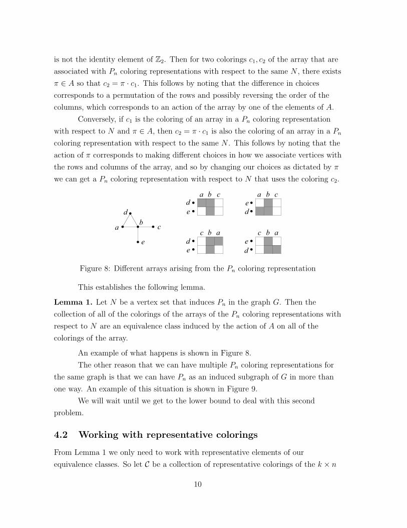
Figure 8: Different arrays arising from the Pn coloring representation

This establishes the following lemma.

Lemma 1. Let N be a vertex set that induces Pn in the graph G. Then the

collection of all of the colorings of the arrays of the Pn coloring representations with

respect to N are an equivalence class induced by the action of A on all of the

colorings of the array.

An example of what happens is shown in Figure 8.

The other reason that we can have multiple Pn coloring representations for

the same graph is that we can have Pn as an induced subgraph of G in more than

one way. An example of this situation is shown in Figure 9.

We will wait until we get to the lower bound to deal with this second

problem.

4.2 Working with representative colorings

From Lemma 1 we only need to work with representative elements of our

equivalence classes. So let C be a collection of representative colorings of the k × n

10

ca

db

fedbfeca

da

fecb

fb

deca

fc

edba

fed

cb

a

Figure 9: A graph with multiple P4 representations

array with two colors, i.e., every coloring of our k × n array is equivalent with

exactly one coloring of C.

So if G is a graph with a Pn coloring representation with respect to N then

the coloring of the array is equivalent to exactly one of the colorings of C. In

particular, by modifying our choices in our Pn coloring representation with respect

to N we get a Pn coloring representation with respect to N of G so that the array

has one of the colorings of C.

It is important to note that we have still not overcome the arbitrariness of

how we choose to associate vertices with the rows and the columns. Ambiguity can

still arise when there is a non-identity element π ∈ A that the coloring is invariant

under. Again, we will examine this in more detail when we come to dealing with the

lower bounds.

5 Counting our inequivalent colorings

The elements of C will form the basis for our upper and lower bounds, so we need to

determine the size of C. This can be most easily achieved by use of Theorem 1

(Burnside’s Lemma).

Before finding the size of C it is useful to examine the structure and

properties of the permutation group on k elements, i.e., Sk. The most important

information for us will be given by the Stirling numbers of the first kind.

5.1 Stirling numbers of the first kind

The Stirling numbers of the first kind, denoted by s(k, i) with i and k non-negative

integers, are defined recursively by

s(k, i) = s(k − 1, i − 1) + (k − 1)s(k − 1, i)

11

with the boundary conditions

s(k, 0) = 0 (k ≥ 1), s(k, k) = 1.

Applying the recursive definition and the boundary conditions to s(k, k) we

have for k ≥ 2 that

s(k, k) = s(k − 1, k − 1) + (k − 1)s(k − 1, k) which yields s(k − 1, k) = 0.

This process can be repeated to show that s(k, i) = 0 whenever k < i.

The Stirling numbers of the first kind, s(k, i), count the number of

permutations of Sk that consist of i cycles in the permutations cycle representation.

This is a consequence of the following theorem found in [3].

Theorem 2. The Stirling number of the first kind, s(k, i), counts the number of

arrangements of k objects into i non-empty circular permutations.

This combined with the following theorem will aid us in counting the number

of inequivalent colorings of C.

Theorem 3. Let s(k, i) denote the Stirling numbers of the first kind. Then

k∑i=1

s(k, i)xi =k−1∏i=0

(x + i).

Proof. Let gk(x) =∑k

i=1 s(k, i)xi. Then the recurrence relationship for the Stirling

numbers of the first kind, along with the boundary conditions, translate into a

recurrence relationship for the functions gk(x). Namely, we have the following.

gk(x) =k∑

i=1

s(k, i)xi =k∑

i=1

(s(k − 1, i − 1) + (k − 1)s(k − 1, i))xi

= xk∑

i=2

s(k − 1, i − 1)xi−1 + (k − 1)k∑

i=1

s(k − 1, i)xi

= x

k−1∑i=1

s(k − 1, i)xi + (k − 1)k−1∑i=1

s(k − 1, i)xi = (x + (k − 1))gk−1(x)

From the boundary conditions for the Stirling numbers of the first kind we have

12

that g1(x) = x and so we have,

k∑i=1

s(k, i)xi = gk(x) = (x + (k − 1))gk−1(x)

= · · · = (x + (k − 1))(x + (k − 2)) · · · (x + 1)g1(x)

= (x + (k − 1))(x + (k − 2)) · · · (x + 1)x =k−1∏i=0

(x + i).

5.2 Counting our inequivalent colorings

Before counting our inequivalent colorings we need to introduce some notation that

will be used in the theorem.

Recall that any element of Sk can be written uniquely up to rearrangement

as the disjoint product of cycles; this is referred to as the cycle representation. So if

σ ∈ Sk then we will let e(σ) denote the number of even cycles in the cycle

representation of σ and o(σ) denote the number of odd cycles in the cycle

representation of σ.

Theorem 4. Let |C| denote the number of representative elements of the colorings

of the array under the action A, i.e., the number of equivalence classes under the

action A. Then

|C| =1

2k!

(∑σ∈Sk

[2n(e(σ)+o(σ)) + 2ne(σ)+�(n+1)/2�o(σ)

])

=1

2k!

(k−1∏i=0

(2n + i) +∑σ∈Sk

2ne(σ)+�(n+1)/2�o(σ)

)

≤ 1

2k!

(k−1∏i=0

(2n + i) + k!2�(n+1)/2�k)

Proof. To apply Burnside’s Lemma we need to determine the number of colorings of

the array that are fixed under the action of π for each π ∈ A. Let π = σ × a where

σ ∈ Sk and a ∈ Z2.

Then, we will determine the number of colorings of the array that are fixed

under π by looking at the behavior of the cycles in the cycle representation of σ in

three cases.

13

(i) A cycle in σ where a is the identity, i.e., we do not reverse the order of the

columns. We can arbitrarily choose the coloring for the row that corresponds

to the first element of our cycle. Then in order for our coloring to remain fixed

every other row corresponding to the elements of the cycle must have the same

coloring. (Imagine that the rows were sequential, then we would color the first

row and then copy the coloring down to every row that corresponded to our

cycle.)

In particular, for every cycle we get to make n choices.

(ii) An even cycle in σ where a is not the identity, i.e., we do reverse the order of

the columns. We choose an arbitrary coloring of the row that corresponds to

the first element of the cycle. Then as we go through the elements of the cycle

we reverse the order and fill in the rows as we go. (Imagine that the rows were

sequential, then we would color the first row and then we would move down

and reverse the row to color the next one and continue the process of moving

down and reversing the row to color in the rest of the rows that corresponded

to our cycle.)

When we return to the row that corresponds to the first element of the cycle

we will have made an even number of reversals and so we will match up with

what we started with. In particular, for every cycle we get to make n choices.

(iii) An odd cycle in σ where a is not the identity, i.e., we do reverse the order of

the columns. We choose an arbitrary coloring of the row that corresponds to

the first element of the cycle. Then as we go through the elements of the cycle

we reverse the order and fill in the rows as we go, as in the previous case.

When we return to the row that corresponds to the first element of the cycle

we will have made an odd number of reversals and in particular will be the

reverse of what we started with. In order to match up with what we started

with (i.e., in order for the coloring to remain fixed) the coloring of the first

row has to be symmetric. In particular, for every cycle we get to make

�(n + 1)/2� choices, that is we get to color half of one row which will then

determine the rest of the coloring for the cycle.

From (i) we have that when π is of the form σ × a and a is the identity then

for every cycle in σ we get n choices and so there are 2n(e(σ)+o(σ)) colorings fixed by π.

14

Combining (ii) and (iii) we have that when π is of the form σ × a and a is

not the identity, then for every even cycle in σ we get n choices and for every odd

cycle in σ we get �(n + 1)/2� choices and so there are 2ne(σ)+�(n+1)/2�o(σ) colorings

fixed by π.

Since A = Sk × Z2 we have that |A| = |Sk| · |Z2| = 2k!. We will now apply

Burnside’s Lemma and get that

|C| =1

2k!

∑σ∈Sk

2n(e(σ)+o(σ))

︸ ︷︷ ︸(I)

+∑σ∈Sk

2ne(σ)+�(n+1)/2�o(σ)

︸ ︷︷ ︸(II)

where the first sum is all elements of π of the form σ × a where a is the identity and

the second sum is all elements of π of the from σ × a where a is not the identity.

Combining these sums gives us our first equality in the conclusion of the theorem.

In (I) note that e(σ) + o(σ) is the number of cycles in σ. If we group the

permutations of Sk according to how many cycles the permutations have then we

will have k groups (for 1, 2, . . . , k) each with s(k, i) elements, where i is the number

of cycles. So we have that

∑σ∈Sk

2n(e(σ)+o(σ)) =k∑

i=1

s(k, i)2ni.

Now applying Theorem 3 with x = 2n we have

k∑i=1

s(k, i)2ni =k−1∏i=0

(2n + i).

Putting this in for (I) we have

|C| =1

2k!

(k−1∏i=0

(2n + i) +∑σ∈Sk

2ne(σ)+�(n+1)/2�o(σ)

)

which gives us our second equality in the conclusion of the theorem.

For (II) note that when σ ∈ Sk that 2e(σ) + o(σ) ≤ k and so

ne(σ) + �(n + 1)/2� o(σ) ≤ �(n + 1)/2� (2e(σ) + o(σ)) ≤ �(n + 1)/2� k.

As an immediate consequence we have∑σ∈Sk

2ne(σ)+�(n+1)/2�o(σ) ≤∑σ∈Sk

2�(n+1)/2�k = k!2�(n+1)/2�k

15

Putting this in for (II), along with what we have already done for (I), we

have

|C| ≤ 1

2k!

(k−1∏i=0

(2n + i) + k!2�(n+1)/2�k)

which gives us our final inequality for the theorem.

Although we have two exact formulas for |C| it is most convenient to use the

bound

|C| ≤ 1

2k!

(k−1∏i=0

(2n + i) + k!2�(n+1)/2�k)

.

While this bound is not sharp it can be calculated without knowing anything about

the elements of Sk.

In addition, asymptotically this bound behaves like the exact formulas. This

is because the first part of the bound (the(∏k−1

i=0 (2n + i))

/(2k!)) is exact and as we

shall see later behaves like 2nk/(2k!) as n gets large while the second term is not

sharp and behaves like 2�(n+1)/2�k/2 which comparatively becomes insignificant as n

gets large.

6 Upper bound

With our bound for the size of C in place we can now give an upper bound for

P(n, k). This is done by bounding the number of Pn coloring representations that

are possible for graphs on n + k vertices as shown in the following theorem.

Theorem 5. We have

P(n, k) ≤ 1

2k!

(k−1∏i=0

(2n + i) + k!2�(n+1)/2�k)

2(k2).

Proof. Let G be any graph on n + k vertices which contains Pn as an induced

subgraph. Then by the discussion that followed Lemma 1 there is a Pn coloring

representation of G that uses one of the colorings of C along with some labeled

graph on k vertices.

In particular, all graphs on n + k vertices which contain Pn as an induced

subgraph are represented at least once (possibly several times) in the combinations

of all k × n arrays which are colored with a coloring of C and all graphs on k labeled

vertices. Since each one of these combinations corresponds to only one graph then

16

the number of graphs on n + k vertices containing Pn as an induced subgraph is at

most the number of these combinations.

There are a total of 2(k2) graphs on k labeled vertices and so there are a total

of |C|2(k2) combinations of colorings of the array with a coloring of C′ with labeled

graphs. Using Theorem 4 we have,

P(n, k) ≤ |C|2(k2) ≤ 1

2k!

(k−1∏i=0

(2n + i) + k!2�(n+1)/2�k)

2(k2).

7 Lower bound

To get our upper bound we created a combination of colorings of the array and

labeled graphs where each graph on n + k vertices which contained Pn as an induced

subgraph was represented at least once. To get our lower bound we will use a

similar approach in that we will create a combination of colorings and labeled

graphs where each graph on n + k vertices which contains Pn as an induced

subgraph will be represented at most once.

In order to obtain a lower bound we will show that by making restrictions on

our colorings that we can overcome two problems that were inherent in our upper

bounds. The first problem is having Pn as an induced subgraph in multiple ways.

The second problem is the colorings of our array which are invariant under multiple

automorphisms.

7.1 Having a long induced path in only one way

In Figure 9 we saw that one graph can have Pn as an induced subgraph in multiple

ways. In looking at all combinations of colorings of C and labeled graphs this caused

some graphs to be counted multiple times. To overcome this problem we will use

the following lemmas.

Lemma 2. Let G = (V,E) and let N ⊆ V induce Pn as a subgraph then for all

v ∈ N we have deg(v) ≤ |V | − n + 2.

Proof. Since the maximum degree of a vertex in Pn is 2, if v ∈ N then v can be

adjacent to at most 2 other vertices of N . In particular v is not adjacent to n − 2 of

17

the vertices of V lying in N . Thus, the maximum degree that v can have is

|V | − (n − 2).

Lemma 3. If the k × n array in a Pn coloring representation of a graph has at least

k + 3 entries in each row colored ‘yes’ then the graph contains Pn as an induced

subgraph in exactly one way.

Proof. Each row corresponds to a vertex in the graph, and by our assumption each

vertex corresponding to a row has degree at least k + 3. By Lemma 2, with

|V | = n + k, it follow that none of the k vertices that correspond to the rows can lie

in an induced subgraph which is Pn. Thus only n of the n + k vertices can lie in an

induced subgraph which is Pn and so we have no more than one way to have Pn as

an induced subgraph.

Since the columns correspond to a Pn which is an induced subgraph we have

at least one way that the graph contains Pn as an induced subgraph.

Combining these two we have exactly one way that the graph contains Pn as

an induced subgraph.

If we add the restriction that our colorings have at least k + 3 or more

elements colored ‘yes’ then from Lemma 3 all of the corresponding graphs with such

colorings can have Pn as an induced subgraph in only one way. In order for the

restriction to be useful we will get a bound on the number of graphs that do not

satisfy this restriction. This will be done with the following lemma.

Lemma 4. Let D be a maximal collection of inequivalent colorings with two colors

of the k × n array under the action of A, such that each coloring of D contains at

least one row with k + 2 or fewer elements colored ‘yes.’ Then

|D| ≤(

k+2∑i=0

(n

i

)) (1

2(k − 1)!

(k−2∏i=0

(2n + i) + (k − 1)!2�(n+1)/2�(k−1)

)).

Proof. Let E denote a maximal collection of inequivalent colorings of the (k − 1)× n

array under the action of the group A′ = Sk−1 × Z2. Now consider the collection of

k × n arrays where the first row contains k + 2 or fewer elements colored ‘yes’ and

the remaining k − 1 rows correspond to a coloring of E .

We claim that every coloring of D is equivalent with at least one coloring in

this collection. To see this start with d ∈ D. Then d is equivalent to a coloring of

the k × n array, call it d′, where the first row has k + 2 or fewer elements colored

18

‘yes’ by an action which permutes the first row with any row which contains k + 2

or fewer elements colored ‘yes.’

The resulting rows 2 through k are a coloring of the (k − 1) × n array and in

particular there is an automorphism in A′ which acts on these k − 1 rows which

takes it to a coloring of E . This automorphism in A′ can be extended to an

automorphism in A that acts on d′ where the first row does not change position

(but possibly might reverse order) and the remaining (k − 1) rows becomes one of

the colorings of E .

In particular we have that d ∈ D is equivalent to a coloring d′ which in turn

is equivalent to a coloring which has k + 2 or fewer elements colored ‘yes’ in the first

row and the remaining k − 1 rows corresponds to a coloring of E .

So we can bound |D| by bounding the number of colorings in this collection.

First note that there are a total of

k+2∑i=0

(n

i

)

different ways that the first row can have k + 2 or fewer elements colored yes.

From Theorem 4 we have that

|E| ≤ 1

2(k − 1)!

(k−2∏i=0

(2n + i) + (k − 1)!2�(n+1)/2�(k−1)

).

Combining these we have that

|D| ≤(

k+2∑i=0

(n

i

)) (1

2(k − 1)!

(k−2∏i=0

(2n + i) + (k − 1)!2�(n+1)/2�(k−1)

)).

7.2 Colorings fixed only under the identity automorphism

A second source for overcounting when we did our upper bound arose because some

colorings of C are invariant under multiple actions. This can cause a graph to have

several distinct labeled graphs associated with a fixed coloring of the array. An

example of this situation is shown in Figure 10.

This occurs because the different actions for which the graph is invariant

corresponds to different sets of choices in how we make our Pn coloring

19

egfh

efgh

abcdabcd

hfge

hgfe

dcbadcba

hg

fe

dcb

a

Figure 10: Representations with a fixed coloring and multiple labeled graphs

representation. In particular, we can have the same coloring of the array but have

changed the labeling of the graph on k vertices.

If we add the restriction that our colorings remain invariant only under the

identity automorphism then we can overcome this problem. In order for this

restriction to be useful we need to get a bound on the number of colorings which

satisfy this restriction. This will be done by breaking the problem into two pieces

and then examining each piece in turn as done in the following lemmas.

Lemma 5. Let D be a maximal collection of inequivalent colorings with two colors

of the k × n array under the action of A such that for each coloring of D there is a

non-identity element π ∈ A where π = σ × a and a is the identity (so we do not

reverse the order of the columns) and for which the coloring is invariant under the

action by π. Then

|D| ≤ (k − 1)

(1

2(k − 1)!

(k−2∏i=0

(2n + i) + (k − 1)!2�(n+1)/2�(k−1)

)).

Proof. Let E denote a maximal collection of inequivalent colorings of the (k − 1)× n

array under the action of the group A′ = Sk−1 × Z2. Now start with any coloring of

E and put the coloring into rows 2 through k of a k × n array. For row 1 put a

duplicate of each of the rows 2 through k in turn, making a total of k − 1 different

colorings (with some possible repetitions) of the k × n array. An example of this

construction is shown in Figure 11.

For every coloring of E we have now constructed k − 1 colorings of the k × n

array, and so we have constructed at most (k − 1)|E| colorings. By application of

Theorem 4 we have that the number of colorings that we have constructed is

20

Figure 11: An example of the construction in Lemma 5

bounded above by

(k − 1)

(1

2(k − 1)!

(k−2∏i=0

(2n + i) + (k − 1)!2�(n+1)/2�(k−1)

)).

All that remains in the proof is to show that each coloring of D is equivalent

to at least one of the colorings that we have constructed.

First note that since we do not reverse the order of the columns that the only

way a coloring can remain invariant under the action of a non-identity element of A

is for there to be a duplicate row in the array.

Let d ∈ D be a coloring. Then d must contain two rows which are duplicated

and in particular we have that d is equivalent to a coloring, d′, in which the first row

is a duplicate of some other row by applying any action of A which takes one of the

duplicate rows to the first row.

Rows 2 through k are a coloring of the (k − 1) × n array and in particular

there is an action in A′ which acts on these k − 1 rows which takes it to a coloring of

E . This action in A′ can be extended to an action in A that acts on d′ where the

first row does not change position (but possibly might reverse order) and the

remaining k − 1 rows becomes one of the colorings of E .

In particular we have that d ∈ D is equivalent to a coloring d′ which in turn

is equivalent to a coloring where rows 2 through k are a coloring in E and the first

row is a duplicate of one of the rows of 2 through k. This completes the proof.

Lemma 6. Let D be a maximal collection of inequivalent colorings of the k × n

array with two colors under the action of the group A such that for each coloring of

D there is an element π ∈ A so that π = σ · a where a is not the identity (so the

effect of the action reverses the order of the columns) so that the coloring is

invariant under π. Then

|D| ≤⌊

k + 2

2

⌋2�(n+1)/2�k.

Proof. Let d ∈ D and consider any row of d. If the row of d is not symmetric then

in order for the coloring to remain invariant under an automorphism which reverses

21

the order of the columns there must be some row which has the coloring in reverse

order. In particular, the rows of d are either symmetric or they can be placed in

pairs which are the reverse order of each other.

Suppose that we have j rows that are paired together. Then the remaining

k − 2j rows must be symmetric. For every pair of rows we get to make a full choice

for one row and the other row will have its coloring determined, so we get a total of

nj choices. For the symmetric rows we get to color half the row and then the other

half must be colored in reverse order to be symmetric and so we get

(k − 2j)�(n + 1)/2� choices.

The number of pairs that we can have is between 0 and �k/2�, so we get

|D| ≤�(k/2)�∑

j=0

2nj+(k−2j)�(n+1)/2�.

Now note that n ≤ 2�(n + 1)/2� so we have

�k/2�∑j=0

2nj+(k−2j)�(n+1)/2� ≤�k/2�∑j=0

22j�(n+1)/2�+(k−2j)�(n+1)/2� =

�k/2�∑j=0

2�(n+1)/2�k

=

(⌊k

2

⌋+ 1

)2�(n+1)/2�k =

⌊k + 2

2

⌋2�(n+1)/2�k.

Any coloring that is invariant under an action which reverses the columns will be

equivalent to one of these, i.e., we permute the rows to put the pairs in order at the

top of the array and the symmetric rows at the bottom. This concludes the

proof.

7.3 The lower bound

The lemmas will provide a way to create a large number of Pn coloring

representations on n + k vertices that correspond to non-isomorphic graphs. This

will establish the lower bound for P(n, k) given by the next theorem.

Theorem 6. Let

S =

(k+2∑i=0

(n

i

)) (1

2(k − 1)!

(k−2∏i=0

(2n + i) + (k − 1)!2�(n+1)/2�(k−1)

))

T = (k − 1)

(1

2(k − 1)!

(k−2∏i=0

(2n + i) + (k − 1)!2�(n+1)/2�(k−1)

))

U =

⌊k + 2

2

⌋2�(n+1)/2�k.

22

Then we have (1

2k!

k−1∏i=0

(2n + i) − S − T − U

)2(k

2) ≤ P(n, k).

Proof. Let D be a maximal collection of inequivalent colorings of the k × n array

where every coloring satisfies the following conditions:

(i) every row of the coloring has at least k + 3 entries colored ‘yes,’

(ii) the only action in A for which the coloring is invariant is the action induced

by the identity element of A.

Then consider all combinations of colorings of the array with colorings of D along

with all graphs on k labeled vertices.

We claim that any graph on n + k vertices which contains Pn as an induced

subgraph is represented at most once in this combination. To see this let G be a

graph on n + k vertices. Then if G has no Pn coloring representation that has the

array colored with a coloring of D then it cannot show up in the combination.

So suppose that the graph does have a Pn coloring representation of G with a

coloring of the array colored with a coloring of D. Then by (i) and Lemma 3 we

know that the graph contains Pn as an induced subgraph in exactly one way, so

there is only one coloring of D which corresponds to a Pn coloring representations of

the graph.

Now note that because of (ii) there is only one possible way of assigning the

vertices to the columns and the rows so that the coloring matches with the coloring

of D. If there were two distinct ways of assigning the vertices to the columns and

the rows then we could form an automorphism that is not the identity for which the

coloring would be invariant, which is impossible by assumption. It follows that for

G there is only one labeled graph that we can associate with the coloring of D. In

particular, G can only show up once in the combination of the colorings of D and all

of the labeled graphs.

Since each graph on n + k vertices which contains Pn as an induced subgraph

is represented at most once in these combinations, and each one of these

combinations corresponds to a graph on n + k vertices which contains Pn as an

induced subgraph, we can conclude that

|D|2(k2) ≤ P(n, k)

23

All that remains is to bound |D|.To bound |D| we will start with a lower bound for the number of

inequivalent colorings of the k × n array and then get an upper bound for the

number of colorings that we need to throw out so that the colorings that remain will

satisfy conditions (i) and (ii).

Our lower bound for the number of inequivalent colorings of the k × n array

comes from Theorem 4. Letting |C| denote the number of inequivalent colorings of

the k × n array we have that

1

2k!

k−1∏i=0

(2n + i) ≤ 1

2k!

(k−1∏i=0

(2n + i) +∑σ∈Sk

2ne(σ)+�(n+1)/2�o(σ)

)= |C|.

Our upper bound for the number of colorings that we need to throw out will

come by combining Lemmas 4, 5 and 6. By Lemma 4, the number of graphs which

do not satisfy (i) is bounded above by S. By Lemmas 5 and 6, the number of graphs

which do not satisfy (ii) is bounded above by T + U . Combining these we have that

the number of graphs which do not satisfy (i) or (ii) is bounded above by S +T +U .

Subtracting our upper bound for the number of colorings that we need to

throw out from our lower bound for the number of inequivalent colorings we can

conclude that1

2k!

k−1∏i=0

(2n + i) − S − T − U ≤ |D|.

This concludes the proof.

8 Asymptotic behavior

Comparing the upper and lower bound we see that as we fix k and let n get large

the term which will dominate in both bounds is the same. In particular we have the

following theorem.

Theorem 7. Let k be fixed. Then

limn→∞

P(n, k)

2nk=

2(k2)

2k!.

Proof. By Theorem 5 we have

P(n, k) ≤ 1

2k!

(k−1∏i=0

(2n + i) + k!2�(n+1)/2�k)

2(k2).

24

Dividing both sides through by 2nk and simplifying we have

P(n, k)

2nk≤ 1

2k!

(k−1∏i=0

(1 + i2−n) + k!2(�(n+1)/2�−n)k

)2(k

2).

Taking the limit as n goes to infinity on both sides we have

lim supn→∞

P(n, k)

2nk≤ 1

2k!

(k−1∏i=0

(1 + 0) + k!(0)

)2(k

2) =2(k

2)

2k!.

By Theorem 6 if we let

S =

(k+2∑i=0

(n

i

)) (1

2(k − 1)!

(k−2∏i=0

(2n + i) + (k − 1)!2�(n+1)/2�(k−1)

))

T = (k − 1)

(1

2(k − 1)!

(k−2∏i=0

(2n + i) + (k − 1)!2�(n+1)/2�(k−1)

))

U =

⌊k + 2

2

⌋2�(n+1)/2�k,

then we have

P(n, k) ≥(

1

2k!

k−1∏i=0

(2n + i) − S − T − U

)2(k

2).

Dividing both sides by 2nk and simplifying we have

P(n, k)

2nk≥

(1

2k!

k−1∏i=0

(1 + i2−n) − S

2nk− T

2nk− U

2nk

)2(k

2).

Consider S/2nk. Simplifying we have that

S

2nk=

(∑k+2i=0

(ni

)2n

) (1

2(k − 1)!

(k−2∏i=0

(1 + i2−n) + (k − 1)!2(�(n+1)/2�−n)(k−1)

)).

Now note that the second term is similar to what we had before and will approach

1/(2(k − 1)!). The top of the first term (the∑k+2

i=0

(ni

)) corresponds to a polynomial

of n with degree k + 2 while the bottom of the first term (the 2n) is an exponential.

So as n gets large the bottom will dominate and drive the first term to zero. In

particular we have that S/2nk goes to zero as n goes to infinity.

Now consider T/2nk. Simplifying we have that

T

2nk=

(k − 1

2n

) (1

2(k − 1)!

(k−2∏i=0

(1 + i2−n) + (k − 1)!2(�(n+1)/2�−n)(k−1)

)).

25

As before the second terms will approach 1/(2(k − 1)!). For the first term (the

(k − 1)/2n) we know that the bottom will dominate and will drive the term to zero.

In particular we have that T/2nk goes to zero as n goes to infinity.

Now consider U/2nk. By the definition of U we have that

U

2nk=

⌊k + 2

2

⌋2(�(n+1)/2�−n)k.

As n gets large the exponent becomes a large negative value and drives the term to

zero. In particular we have that U/2nk goes to zero as n goes to infinity.

So we have

lim infn→∞

P(n, k)

2nk≥ lim

n→∞

(1

2k!

k−1∏i=0

(1 + i2−n) − S

2nk− T

2nk− U

2nk

)2(k

2) =2(k

2)

2k!.

Combining the two results concludes the proof.

As an immediate consequence of the theorem we have that if k is fixed that

P(n, k) ∼ 2(nk+(k2))

2k!.

Conclusion

By using the techniques of Polya counting on a k × n array with two colors we have

been able to find upper and lower bounds for the number of non-isomorphic graphs

on n + k vertices which contain Pn as an induced subgraph. Further, these upper

and lower bounds both grow at the same rate as n gets large for a fixed value of k.

We noted earlier that finding P(19, 4) would be difficult to do by examining

all of the graphs on 23 vertices. With the techniques of this thesis, we can now say

that (6.70802)1022 ≤ P(19, 4) ≤ (1.0075)1023. In this example we can also see that

graphs which contain very long paths as induced subgraphs are rare. Comparing the

upper bound that we have for P(19, 4) with the number of graphs on 23 vertices

(given earlier) we see that for every graph with contains P19 as an induced subgraph

there are at least (5.558)1030 graphs which don’t.

26

References

[1] G. Bacso and Z. Tuza, A characterization of graphs without long induced paths,

Journal of Graph Theory 14 (1990) no.4, 455-464.

[2] B. Bollobas, Modern Graph Theory, Springer, 1998.

[3] R. Brualdi, Introductory Combinatorics (3rd ed), Prentice Hall, 1999.

[4] J. Dong, Some results on graphs without long induced paths, Journal of Graph

Theory 22 (1996) no.1, 23-28.

[5] D. Dummit, R. Foote, Abstract Algebra (2nd ed), Wiley, 1999.

[6] F. Harary and E. Palmer, Graphical Enumeration, Academic Press, 1973.

[7] K. Harris, J. Hirst and M. Mossinghoff, Combinatorics and Graph Theory,

Springer, 2000.

[8] G. Woeginger, J. Sgall, The complexity of coloring graphs without long induced

paths, Acta Cybernetica 15 (2001) no. 1, 107-117.

27