bounds on p-values for a class of stopping rules

Statistics & Probability Letters 48 (2000) 385–392

Bounds on p-values for a class of stopping rules

Jim BishopBryant College, 1150 Douglas Pike, Suite C, Smith�eld RI 02917-1284, USA

Received June 1997; received in revised form October 1999

Abstract

Suppose that Bernoulli trials with unknown stopping rule terminate in s successes and f failures. For a sensible class ofstopping rules, the p-value for a one-sided test is bounded between the negative binomial p-value and twice the binomialp-value for this data. c© 2000 Elsevier Science B.V. All rights reserved

1. Introduction

Consider a series of independent identically distributed Bernoulli trials with probability of success �, andthe following null and alternative hypothesis:

H0: �= 12 H1: �¿ 1

2 :

Suppose the observed outcome is s successes and f failures. The p-value associated with this observationdepends on the stopping rule used to obtain it. For example, Lindley and Phillips (1976) demonstrate thedi�erence in p-values between the binomial (stop after s + f trials) and negative binomial (stop after ffailures) stopping rules. According to the likelihood principle (Berger, 1985), two di�erent stopping rulesresulting in the same values of s and f should not lead to di�erent conclusions about �, so the dependenceof p-value on stopping rule can be viewed as a weakness of p-values as a measure of “signi�cance”. Keener(1988) recommended using the supremum of p-values over all stopping rules in some class, but Berger andBerry (1988) responded that the supremum might be very large for sensible classes.In this paper we �nd bounds on the p-value of Bernoulli experiments by restricting to a natural

class of stopping rules �: We require that the p-value, computed using the likelihood ratio statistic forH0: �= 1

2 vs: H1: �=�1, not depend on the value of �1 (for �1¿12 ). We �nd a simple geometric condition on

the stopping rule that is equivalent to this restriction. For � in this class, the p-value is essentially constrainedbetween an upper bound of twice the binomial p-value and a lower bound equal to the negative binomialp-value.After a section of background and de�nitions, we state and explain the main results in Section 3; proofs

are in Section 4, and a brief discussion is in Section 5.

0167-7152/00/$ - see front matter c© 2000 Elsevier Science B.V. All rights reservedPII: S0167 -7152(00)00020 -1

386 J. Bishop / Statistics & Probability Letters 48 (2000) 385–392

2. Background and de�nitions

Let �1; �2; �3; : : : be independent random variables, where

P�(�i =+1) = �= 1− P�(�i =−1) and Wn = �1 + �2 + · · ·+ �n:Note that Wn is the number of successes minus the number of failures up to time n. Let � be a (nonrandomized)stopping rule. De�ne (n; w) to be a stop point if P�(�= n and Wn = w)¿ 0; this de�nition does not dependon which � ∈ (0; 1) is used. Let A� be the set of all stop points for the rule �.For testing H0: �= 1

2 vs: H1: �= �1, the likelihood ratio at a point (n; w) is given by

�(�1; n; w) = 2n�(n+w)=21 (1− �1)(n−w)=2 (1)

independent of the stopping rule. We de�ne the rejection region with respect to a stop point (n∗; w∗) by

R(�1; n∗; w∗) = {(n; w) ∈ A�: �(�1; n; w)¿�(�1; n∗; w∗)}: (2)

The p-value associated with (n∗; w∗) is

P1=2(�(�1; �; W�)¿�(�1; n∗; w∗)) = P1=2((�;W�) ∈ R(�1; n∗; w∗))

which might depend on �1, of course. Note that we do not require rules to stop with probability one. HenceforthP1=2 is denoted P.We conclude this section with three important examples of stopping rules (see Fig. 1).

(i) Binomial: De�ne �1 ≡ n∗. The p-value associated with (n∗; w∗) is

P(Wn∗¿w∗)

which is the probability that a Binomial (n∗; 12 ) random variable is at least 12 (n∗ + w∗).

(ii) Negative Binomial: Let f∗ be the desired number of failures, and de�ne

�2 = min{n: Wn = n− 2f∗}:If (n∗; w∗) is a stop point, then w∗=n∗−2f∗. The p-value associated with (n∗; w∗) is P(�2¿n∗), whichis the probability that a NegBin(f∗; 12 ) random variable is at least n∗. An exact relation between thenegative binomial and binomial p-values for the stop point (n∗; w∗) can be attained by observing that

P(�2¿n∗) = P(Wn∗−1¿n∗ − 2f∗)

and

P(Wn∗¿n∗ − 2f∗) = P(Wn∗−1¿n∗ − 2f∗) + 12P(Wn∗−1 = n

∗ − 2f∗ − 1):

Fig. 1. Three examples of stopping rules.

J. Bishop / Statistics & Probability Letters 48 (2000) 385–392 387

Thus for the point (n∗; w∗) with w∗ = n∗ − 2f∗ we have

P(Wn∗¿w∗) = P(�2¿n∗) + 12P(Wn∗−1 = w

∗ − 1)so that the binomial p-value for (n∗; w∗) is always greater than the negative binomial p-value, but theymust be close for large n∗.

(iii) Success-minus-failure: De�ne

�3 = min{n: Wn = w∗}:The p-value for a stop point (n∗; w∗) is P(�36n∗), and by the re ection principle

P(�36n∗) = 2P(Wn¿w∗)− P(Wn = w∗)

showing that the success-minus-failure p-value is less than twice the binomial p-value.

3. Main results

We will restrict ourselves to stopping rules satisfying the following:Uniformity condition. A stopping rule � satis�es the uniformity condition if and only if, for all stopping

points (n∗; w∗), the critical region R(�1; n∗; w∗) does not depend on �1 (for �1¿ 12 ).

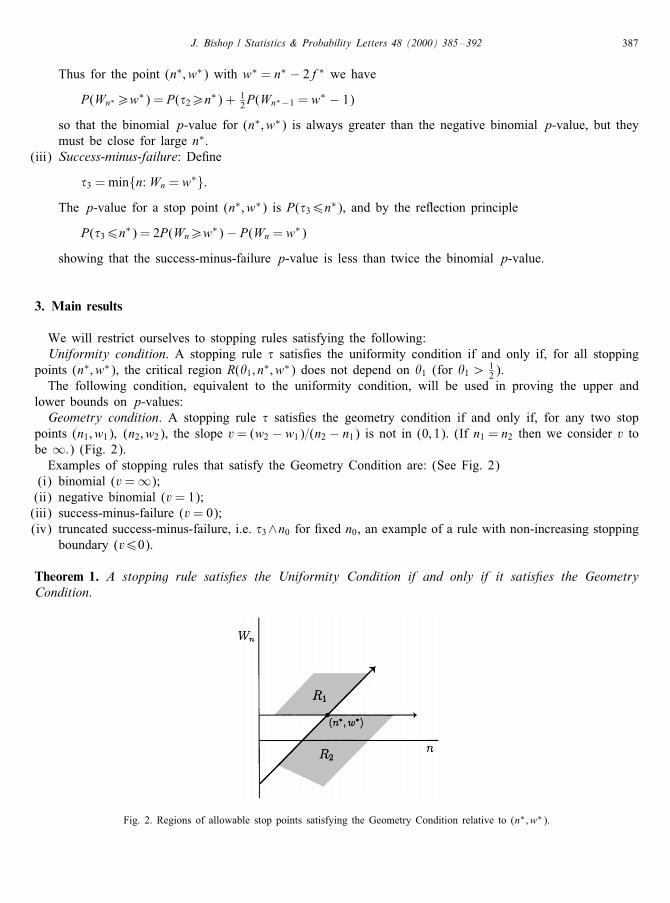
The following condition, equivalent to the uniformity condition, will be used in proving the upper andlower bounds on p-values:Geometry condition. A stopping rule � satis�es the geometry condition if and only if, for any two stop

points (n1; w1); (n2; w2), the slope v= (w2 − w1)=(n2 − n1) is not in (0; 1). (If n1 = n2 then we consider v tobe ∞.) (Fig. 2).Examples of stopping rules that satisfy the Geometry Condition are: (See Fig. 2)

(i) binomial (v=∞);(ii) negative binomial (v= 1);(iii) success-minus-failure (v= 0);(iv) truncated success-minus-failure, i.e. �3∧n0 for �xed n0, an example of a rule with non-increasing stopping

boundary (v60).

Theorem 1. A stopping rule satis�es the Uniformity Condition if and only if it satis�es the GeometryCondition.

Fig. 2. Regions of allowable stop points satisfying the Geometry Condition relative to (n∗; w∗).


Theorem 2 (Upper bound). Let � be a stopping rule satisfying the Uniformity Condition. Then the p-valuefor a stop point (n∗; w∗); is less than or equal to the success-minus-failure p-value; that is;

P(�(�1; �; W�)¿�(�1; n∗; w∗))6P(�36n∗)¡ 2P(Wn∗¿w∗):

A lower bound cannot be obtained without further restriction on the class of permitted stopping rules.Imagine a rule that stops only at (n∗; w∗). The p-value associated with that point could be arbitrarily small(relative to the corresponding binomial p-value, say). So we will impose the following:Stopping condition. A rule satis�es the stopping condition if and only if for some �1¿ 1

2 ; P�1 (�¡∞)=1.

Theorem 3 (Lower bound). Let � be a stopping rule satisfying the Uniformity and Stopping Conditions.Then for any stop point (n∗; w∗) with w∗¿ 0; the p-value is greater than or equal to the negative binomialp-value. Equivalently;

P(�(�1; �; W�)¿�(�1; n∗; w∗))¿P(�2¿n∗):

We conclude this section with an outline of the proofs of Theorems 2 and 3.Suppose that we have proven Theorem 1. It follows that if (n∗; w∗) is a stop point for a rule satisfying the

Uniformity Condition then all stop points are in R1 ∪ R2, whereR1 = {(n; w): w¿w∗ and n− w6n∗ − w∗} (3)

and

R2 = {(n; w): w6w∗ and n− w6n∗ − w∗} \ {(n∗; w∗)}:Furthermore, the p-value can be seen to be

P(�(�1; �; W�)¿�(�1; n∗; w∗)) = P((�;W�) ∈ R1):To maximize P((�;W�) ∈ R1); we de�ne � to stop as soon as (n;Wn) enters R1. This leads to the success-minus-failure rule and Theorem 2.To prove Theorem 3, we try to minimize P((�;W�) ∈ R1) by de�ning � to stop in R1 only if absolutely

necessary to satisfy the requirements of the Stopping Condition. This means that the rule must stop at (n∗ +k; w∗ + k) for k¿2 (if it reaches these points) because otherwise there is a chance of never again enteringR1 ∪ R2 if �1¿ 1

2 . (This is the content of Lemma 5a.) This almost yields the negative binomial rule, whichstops at the points (n∗ ± k; w∗ ± k); except for the nuisance of (n∗ + 1; w∗ + 1). The rule � need not stop at(n∗ + 1; w∗ + 1) as long as it stops at (n∗ + 2; w∗), which is in R2. (If it did not stop at (n∗ + 2; w∗) thenagain the Stopping Condition would fail; see Lemma 5b).So there are two cases to consider. If (n∗+2; w∗) is not a stop point, then (n∗+1; w∗+1) must be a stop

point (if it can be reached), and the negative binomial rule minimizes P((�;W�) ∈ R1). If (n∗ + 2; w∗) is astop point and (n∗ + 1; w∗ + 1) is not, then a slightly di�erent lower bound is attained. A direct comparisonshows that the negative binomial yields the smallest p-value.

4. Proofs of main results

Lemma 4. Let (n1; w1) and (n2; w2) be any two points such that n2¿n1 and let v = (w2 − w1)=(n2 − n1).Then:(a) v¿1⇔ �(�1; n2; w2)¿�(�1; n1; w1) ∀�1¿ 1

2 ;(b) v60⇔ �(�1; n2; w2)6�(�1; n1; w1) ∀�1¿ 1

2 .


Proof. By (1), and w2 = w1 + v(n2 − n1), we have�(�1; n2; w2) = 2n2�

(n2+w1+v(n2−n1))=21 (1− �1)(n2−w1−v(n2−n1))=2

so

�(�1; n2; w2)¿�(�1; n1; w1)⇔ 4�(1+v)1 (1− �1)(1−v)¿1: (4)

Solving for v we �nd that (4) is equivalent to

v¿ln(4�1(1− �1))=ln((1− �1)=�1): (5)

Observe that g(�1) = ln(4�1(1− �1))=ln((1− �1)=�1) is an increasing function of �1 for �1 ∈ ( 12 ; 1) and thatlim�1→ 1

2

g(�1) = 0 and lim�1→1

g(�1) = 1:

Thus (a) and (b) follow from (5).

Proof of Theorem 1. Suppose v= (w2 − w1)=(n2 − n1) 6∈ (0; 1) for any two stop points (n1; w1) and (n2; w2)of �. By Lemma 4, the sets de�ned in (2) do not depend on �1, and � satis�es the Uniformity Condition.Conversely, if there exist stop points (n1; w1) and (n2; w2) such that v= (w2 − w1)=(n2 − n1) ∈ (0; 1); then

by Lemma 4,

∃�′1 with �(�′1; n1; w1)¿�(�′1; n2; w2)

and

∃�′′1 with �(�′′1 ; n1; w1)¡�(�′′1 ; n2; w2)

and therefore the sets in (2) do depend on �1.

Proof of Theorem 2. By Lemma 4, {�(�1; n; w)¿�(�1; n∗; w∗); ∀�1¿ 12} = R1 de�ned in (3). Thus the

p-value associated with (n∗; w∗) is P((�;W�)∈R1) and we will show {(�;W�) ∈ R1}⊆{�36n∗} where �3 =min{n: Wn¿w∗} is the success-minus-failure stopping rule. (Fig. 2 should be convincing.) Write R1=R′1∪R′′1with

R′1 = {(n; w): n6n∗; w¿w∗}and

R′′1 = {(n; w): n¿n∗; n− n∗6w − w∗}:If (�;W�) ∈ R′1, then �6n∗ and W�¿w∗; so �36n∗. If (�;W�) ∈ R′′1 , then �¿n∗ and �− n∗6W�−w∗. SinceW� −Wn∗6� − n∗ for �¿n∗, it follows that W� −Wn∗6W� − w∗ and so Wn∗¿w∗, which implies �36n∗.Therefore, {(�;W�) ∈ R1}⊆{�36n∗} as desired.

Lemma 5. Suppose (n∗; w∗) is a stop point for a rule � satisfying the Geometry and Stopping Conditions.Then for any � ∈ [ 12 ; 1);(a) P�(Wn∗+k = w∗ + k and �¿n∗ + k) = 0 ∀k¿2; and(b) P�(Wn∗+2 = w∗ and �¿n∗ + 2) = 0:

Proof of Lemma 5a. Assume ∃k¿2 such thatP�(Wn∗+k = w∗ + k and �¿n∗ + k)¿ 0

for some 126�¡ 1. This implies

P�(Wn∗+k = w∗ + k and �¿n∗ + k)¿ 0


Fig. 3.

for all 126�¡ 1, since the event is in �(�1; �2; : : : ; �n∗+k). Now, consider

I1 = {Wn∗+k = w∗ + k; �¿n∗ + k}∩{�n∗+k+1 =−1}∩{Wn −Wn∗+k+1¿0;∀n¿n∗ + k + 1}:

Note that (see Fig. 3)

{Wn∗+k = w∗ + k; �¿n∗ + k} ∩ {�n∗+k+1 =−1}⊆{(�;W�) 6∈ R1}:Also,

I1⊆{�¿n∗ + k} ∩ {Wn¿w∗;∀n¿n∗ + k}⊆{(�;W�) 6∈ R2}:Thus I1⊆{(�;W�) 6∈ R1 ∪ R2}, which implies

I1⊆{�=∞} and soP�(I1)6P�(�=∞) for any 1

26�¡ 1:

Since {Wn −Wn∗+k+1¿0;∀n¿n∗ + k + 1} ∈ �(�n∗+k+2; �n∗+k+3; : : :) we have independence andP�(I1) = P�(Wn∗+k = w∗ + k; �¿n∗ + k)

×P�(�n∗+k+1 =−1)×P�(Wn −Wn∗+k+1¿0;∀n¿n∗ + k + 1)

implying P�(I1)¿ 0 for all �¿ 12 . (Note that the �rst factor on the right-hand side is positive by assumption

and the third factor is positive for all �¿ 12 .) Therefore, P�(� =∞)¿ 0; ∀�¿ 1

2 and this contradicts theStopping Condition.

Proof of Lemma 5b. The proof is almost the same as for Lemma 5a. For 5b, de�ne

I2 = {Wn∗+2 = w∗; �¿n∗ + 2}∩{�n∗+3 = +1}∩{Wn −Wn∗+3¿0;∀n¿n∗ + 3}:


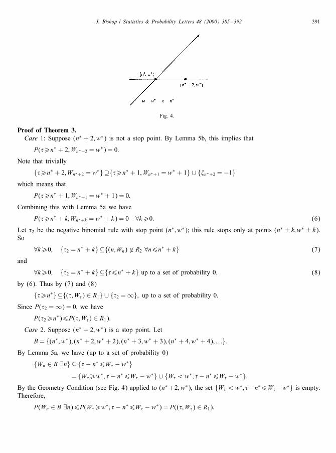
Fig. 4.

Proof of Theorem 3.Case 1: Suppose (n∗ + 2; w∗) is not a stop point. By Lemma 5b, this implies that

P(�¿n∗ + 2; Wn∗+2 = w∗) = 0:

Note that trivially

{�¿n∗ + 2; Wn∗+2 = w∗}⊇{�¿n∗ + 1; Wn∗+1 = w∗ + 1} ∪ {�n∗+2 =−1}which means that

P(�¿n∗ + 1; Wn∗+1 = w∗ + 1) = 0:

Combining this with Lemma 5a we have

P(�¿n∗ + k;Wn∗+k = w∗ + k) = 0 ∀k¿0: (6)

Let �2 be the negative binomial rule with stop point (n∗; w∗); this rule stops only at points (n∗ ± k; w∗ ± k).So

∀k¿0; {�2 = n∗ + k}⊆{(n;Wn) 6∈ R2 ∀n6n∗ + k} (7)

and

∀k¿0; {�2 = n∗ + k}⊆{�6n∗ + k} up to a set of probability 0: (8)

by (6). Thus by (7) and (8)

{�¿n∗}⊆{(�;W�) ∈ R1} ∪ {�2 =∞}; up to a set of probability 0:Since P(�2 =∞) = 0; we have

P(�2¿n∗)6P(�;W�) ∈ R1):Case 2. Suppose (n∗ + 2; w∗) is a stop point. Let

B= {(n∗; w∗); (n∗ + 2; w∗ + 2); (n∗ + 3; w∗ + 3); (n∗ + 4; w∗ + 4); : : :}:By Lemma 5a, we have (up to a set of probability 0)

{Wn ∈ B ∃n} ⊆ {�− n∗6W� − w∗}= {W�¿w∗; �− n∗6W� − w∗} ∪ {W�¡w∗; �− n∗6W� − w∗}:

By the Geometry Condition (see Fig. 4) applied to (n∗+2; w∗), the set {W�¡w∗; �−n∗6W�−w∗} is empty.Therefore,

P(Wn ∈ B ∃n)6P(W�¿w∗; �− n∗6W� − w∗) = P((�;W�) ∈ R1):


It remains to compare P(Wn ∈ B ∃n) from Case 2 with P(�2¿n∗) from Case 1. We have

P(Wn ∈ B ∃n) = P(�2¿n∗)− P(Wn = w∗ + 2; Wn+1 = w∗ + 1; Wn+2 = w∗)

+P(Wn−1 = w∗ − 1; Wn = w∗)

= P(�2¿n∗)− 14P(Wn = w

∗ + 2) + 12P(Wn−1 = w

∗ − 1)and a simple computation with binomial probabilities shows that

P(Wn ∈ B ∃n)¿P(�2¿n∗) if w∗¿0

which was assumed. Thus in both cases, P((�;W�) ∈ R1)¿P(�2¿n∗) and the proof is complete.

5. Conclusion and discussion

We have identi�ed the class of stopping rules for which the p-value computed using likelihood ratio doesnot depend on �1. For this class of stopping rules we have shown that Keener’s suggestion of taking thesupremum is reasonable. The two particular experiments that bound p-values are the negative binomial andthe success-minus-failure experiments.An interesting example of a stopping rule that does not satisfy the Geometry Condition is the rule that stops

when some �xed binomial signi�cance level has been attained. Such rules have the unnerving property thattheir p-values, when calculated using the likelihood ratio statistic, depend heavily on the alternative hypothesis(Bishop, 1999).

References

Berger, J., 1985. Statistical Decision Theory and Bayesian Analysis. Springer, New York.Berger, J.O., Berry, D.A., 1988. The relevance of stopping rules in statistical inference. In: Gupta, S.S., Berger, J. (Eds.), StatisticalDecision Theory & Related Topics IV, Vol. 1. Springer, New York, pp. 29–48.

Bishop, J., 1999. P-values for Stop when Signi�cance is Attained. Preprint.Keener, R., 1988. Discussion. In: Gupta, S.S., Berger, J. (Eds.), Statistical Decision Theory & Related Topics IV, Vol. 1. Springer,New York, pp. 49–56.

Lindley, D.V., Phillips, L.D., 1976. Inference for a Bernoulli process (a Bayesian view). Amer. Statist. 30, 112–119.

bounds on p-values for a class of stopping rules

Documents