boyce/diprima 9th ed, ch 7.5: homogeneous linear systems with
TRANSCRIPT

Boyce/DiPrima 9th ed, Ch 7.5: Homogeneous Linear Systems with Constant Coefficients ���
Elementary Differential Equations and Boundary Value Problems, 9th edition, by William E. Boyce and Richard C. DiPrima, ©2009 by John Wiley & Sons, Inc.
! We consider here a homogeneous system of n first order linear equations with constant, real coefficients:
! This system can be written as x' = Ax, where
Equilibrium Solutions
! Note that if n = 1, then the system reduces to
! Recall that x = 0 is the only equilibrium solution if a ≠ 0. ! Further, x = 0 is an asymptotically stable solution if a < 0,
since other solutions approach x = 0 in this case. ! Also, x = 0 is an unstable solution if a > 0, since other
solutions depart from x = 0 in this case. ! For n > 1, equilibrium solutions are similarly found by
solving Ax = 0. We assume detA ≠ 0, so that x = 0 is the only solution. Determining whether x = 0 is asymptotically stable or unstable is an important question here as well.
Phase Plane
! When n = 2, then the system reduces to
! This case can be visualized in the x1x2-plane, which is called the phase plane.
! In the phase plane, a direction field can be obtained by evaluating Ax at many points and plotting the resulting vectors, which will be tangent to solution vectors.
! A plot that shows representative solution trajectories is called a phase portrait.
! Examples of phase planes, directions fields and phase portraits will be given later in this section.

Solving Homogeneous System
! To construct a general solution to x' = Ax, assume a solution of the form x = ξert, where the exponent r and the constant vector ξ are to be determined.
! Substituting x = ξert into x' = Ax, we obtain
! Thus to solve the homogeneous system of differential equations x' = Ax, we must find the eigenvalues and eigenvectors of A.
! Therefore x = ξert is a solution of x' = Ax provided that r is an eigenvalue and ξ is an eigenvector of the coefficient matrix A.
Example 1: Direction Field (1 of 9)
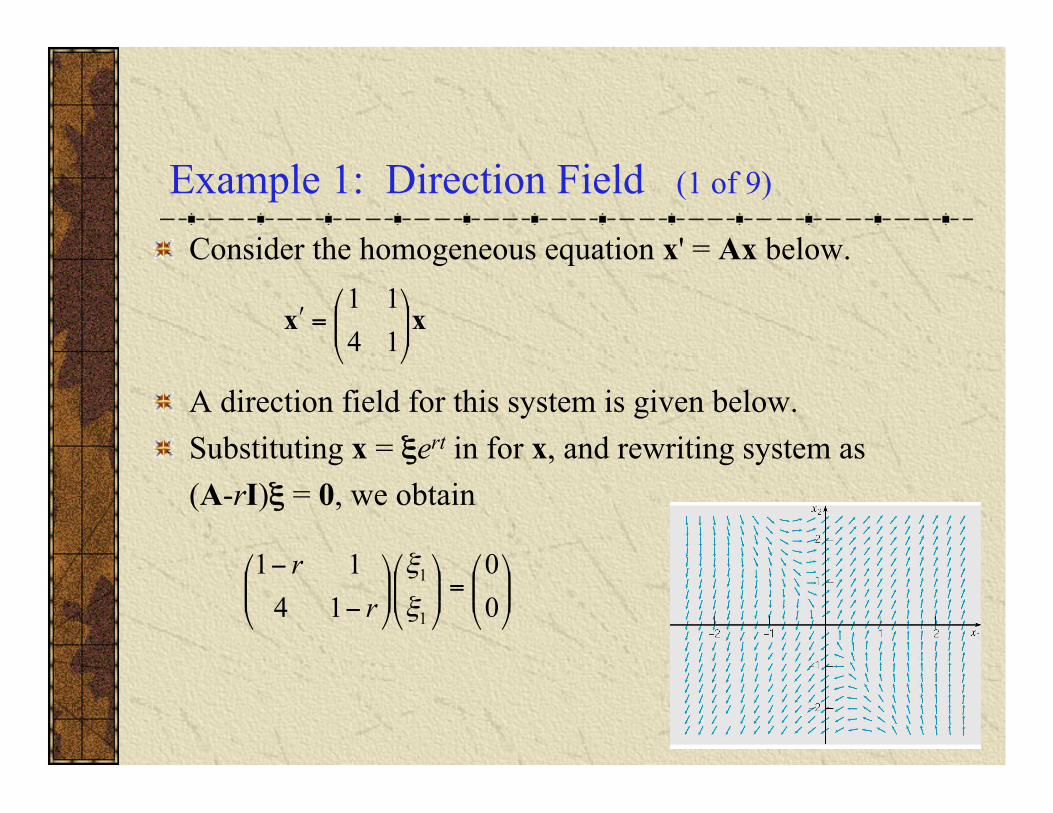
! Consider the homogeneous equation x' = Ax below.
! A direction field for this system is given below. ! Substituting x = ξert in for x, and rewriting system as
(A-rI)ξ = 0, we obtain
Example 1: Eigenvalues (2 of 9)
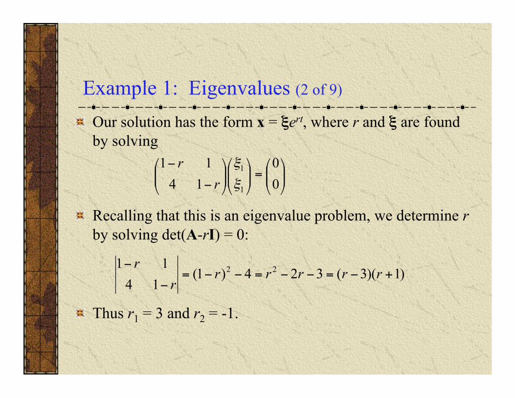
! Our solution has the form x = ξert, where r and ξ are found by solving
! Recalling that this is an eigenvalue problem, we determine r by solving det(A-rI) = 0:
! Thus r1 = 3 and r2 = -1.

Example 1: First Eigenvector (3 of 9)
! Eigenvector for r1 = 3: Solve
by row reducing the augmented matrix:

Example 1: Second Eigenvector (4 of 9)
! Eigenvector for r2 = -1: Solve
by row reducing the augmented matrix:

Example 1: General Solution (5 of 9)
! The corresponding solutions x = ξert of x' = Ax are
! The Wronskian of these two solutions is
! Thus x(1) and x(2) are fundamental solutions, and the general solution of x' = Ax is

Example 1: Phase Plane for x(1) (6 of 9)
! To visualize solution, consider first x = c1x(1):
! Now
! Thus x(1) lies along the straight line x2 = 2x1, which is the line through origin in direction of first eigenvector ξ(1)
! If solution is trajectory of particle, with position given by (x1, x2), then it is in Q1 when c1 > 0, and in Q3 when c1 < 0.
! In either case, particle moves away from origin as t increases.

Example 1: Phase Plane for x(2) (7 of 9)
! Next, consider x = c2x(2):
! Then x(2) lies along the straight line x2 = -2x1, which is the line through origin in direction of 2nd eigenvector ξ(2)
! If solution is trajectory of particle, with position given by (x1, x2), then it is in Q4 when c2 > 0, and in Q2 when c2 < 0.
! In either case, particle moves towards origin as t increases.
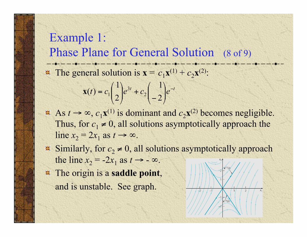
Example 1: Phase Plane for General Solution (8 of 9)
! The general solution is x = c1x(1) + c2x(2):
! As t → ∞, c1x(1) is dominant and c2x(2) becomes negligible. Thus, for c1 ≠ 0, all solutions asymptotically approach the line x2 = 2x1 as t → ∞.
! Similarly, for c2 ≠ 0, all solutions asymptotically approach the line x2 = -2x1 as t → - ∞.
! The origin is a saddle point, and is unstable. See graph.
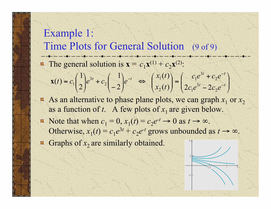
Example 1: Time Plots for General Solution (9 of 9)
! The general solution is x = c1x(1) + c2x(2):
! As an alternative to phase plane plots, we can graph x1 or x2 as a function of t. A few plots of x1 are given below.
! Note that when c1 = 0, x1(t) = c2e-t → 0 as t → ∞. Otherwise, x1(t) = c1e3t + c2e-t grows unbounded as t → ∞.
! Graphs of x2 are similarly obtained.

Example 2: Direction Field (1 of 9)
! Consider the homogeneous equation x' = Ax below.
! A direction field for this system is given below. ! Substituting x = ξert in for x, and rewriting system as
(A-rI)ξ = 0, we obtain
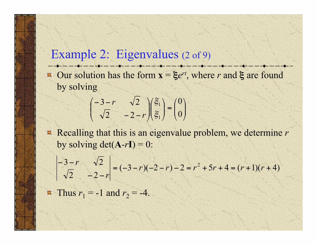
Example 2: Eigenvalues (2 of 9)
! Our solution has the form x = ξert, where r and ξ are found by solving
! Recalling that this is an eigenvalue problem, we determine r by solving det(A-rI) = 0:
! Thus r1 = -1 and r2 = -4.

Example 2: First Eigenvector (3 of 9)
! Eigenvector for r1 = -1: Solve
by row reducing the augmented matrix:
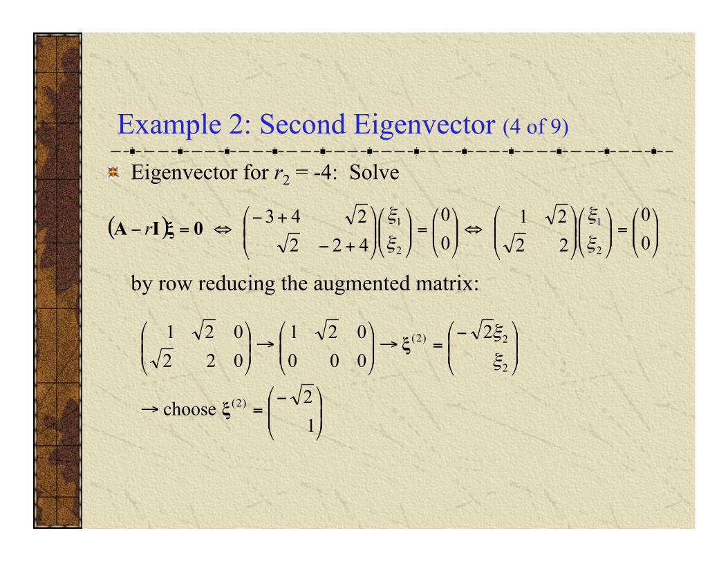
Example 2: Second Eigenvector (4 of 9)
! Eigenvector for r2 = -4: Solve
by row reducing the augmented matrix:

Example 2: General Solution (5 of 9)
! The corresponding solutions x = ξert of x' = Ax are
! The Wronskian of these two solutions is
! Thus x(1) and x(2) are fundamental solutions, and the general solution of x' = Ax is
Example 2: Phase Plane for x(1) (6 of 9)
! To visualize solution, consider first x = c1x(1):
! Now
! Thus x(1) lies along the straight line x2 = 2½ x1, which is the line through origin in direction of first eigenvector ξ(1)
! If solution is trajectory of particle, with position given by (x1, x2), then it is in Q1 when c1 > 0, and in Q3 when c1 < 0.
! In either case, particle moves towards origin as t increases.

Example 2: Phase Plane for x(2) (7 of 9)
! Next, consider x = c2x(2):
! Then x(2) lies along the straight line x2 = -2½ x1, which is the line through origin in direction of 2nd eigenvector ξ(2)
! If solution is trajectory of particle, with position given by (x1, x2), then it is in Q4 when c2 > 0, and in Q2 when c2 < 0.
! In either case, particle moves towards origin as t increases.
Example 2: Phase Plane for General Solution (8 of 9)
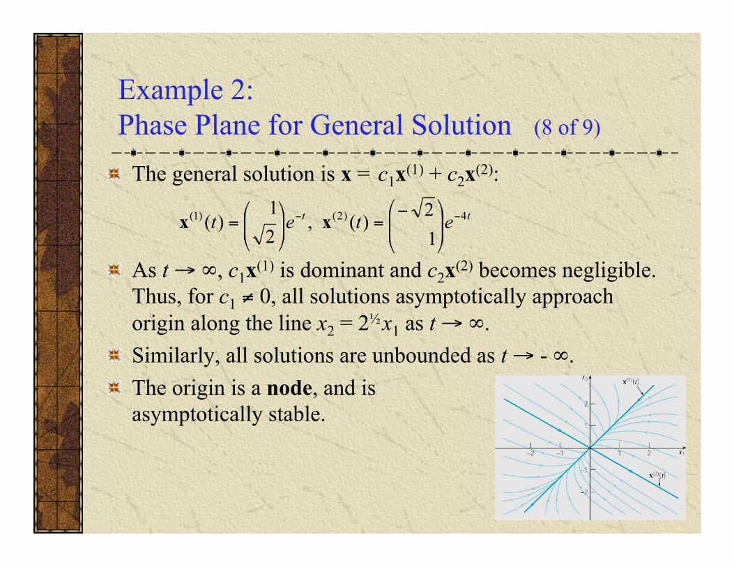
! The general solution is x = c1x(1) + c2x(2):
! As t → ∞, c1x(1) is dominant and c2x(2) becomes negligible. Thus, for c1 ≠ 0, all solutions asymptotically approach origin along the line x2 = 2½ x1 as t → ∞.
! Similarly, all solutions are unbounded as t → - ∞. ! The origin is a node, and is
asymptotically stable.
Example 2: Time Plots for General Solution (9 of 9)
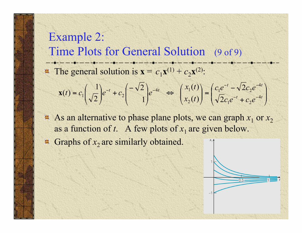
! The general solution is x = c1x(1) + c2x(2):
! As an alternative to phase plane plots, we can graph x1 or x2 as a function of t. A few plots of x1 are given below.
! Graphs of x2 are similarly obtained.

2 x 2 Case: Real Eigenvalues, Saddle Points and Nodes
! The previous two examples demonstrate the two main cases for a 2 x 2 real system with real and different eigenvalues: ! Both eigenvalues have opposite signs, in which case origin is a
saddle point and is unstable. ! Both eigenvalues have the same sign, in which case origin is a node,
and is asymptotically stable if the eigenvalues are negative and unstable if the eigenvalues are positive.

Eigenvalues, Eigenvectors and Fundamental Solutions
! In general, for an n x n real linear system x' = Ax: ! All eigenvalues are real and different from each other. ! Some eigenvalues occur in complex conjugate pairs. ! Some eigenvalues are repeated.
! If eigenvalues r1,…, rn are real & different, then there are n corresponding linearly independent eigenvectors ξ(1),…, ξ(n). The associated solutions of x' = Ax are
! Using Wronskian, it can be shown that these solutions are linearly independent, and hence form a fundamental set of solutions. Thus general solution is

Hermitian Case: Eigenvalues, Eigenvectors & Fundamental Solutions
! If A is an n x n Hermitian matrix (real and symmetric), then all eigenvalues r1,…, rn are real, although some may repeat.
! In any case, there are n corresponding linearly independent and orthogonal eigenvectors ξ(1),…, ξ(n). The associated solutions of x' = Ax are
and form a fundamental set of solutions.

Example 3: Hermitian Matrix (1 of 3)
! Consider the homogeneous equation x' = Ax below.
! The eigenvalues were found previously in Ch 7.3, and were: r1 = 2, r2 = -1 and r3 = -1.
! Corresponding eigenvectors:
Example 3: General Solution (2 of 3)
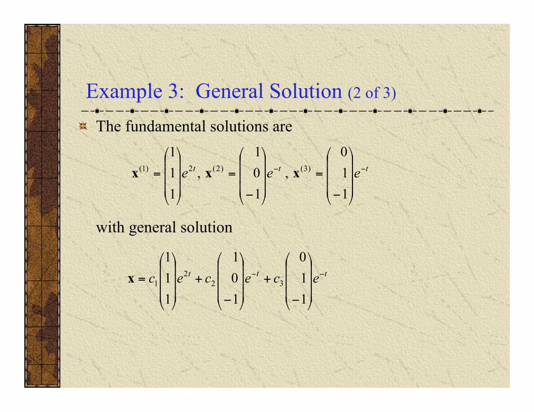
! The fundamental solutions are
with general solution

Example 3: General Solution Behavior (3 of 3)
! The general solution is x = c1x(1) + c2x(2) + c3x(3):
! As t → ∞, c1x(1) is dominant and c2x(2) , c3x(3) become negligible.
! Thus, for c1 ≠ 0, all solns x become unbounded as t → ∞, while for c1 = 0, all solns x → 0 as t → ∞.
! The initial points that cause c1 = 0 are those that lie in plane determined by ξ(2) and ξ(3). Thus solutions that start in this plane approach origin as t → ∞.

Complex Eigenvalues and Fundamental Solns ! If some of the eigenvalues r1,…, rn occur in complex
conjugate pairs, but otherwise are different, then there are still n corresponding linearly independent solutions
which form a fundamental set of solutions. Some may be complex-valued, but real-valued solutions may be derived from them. This situation will be examined in Ch 7.6.
! If the coefficient matrix A is complex, then complex eigenvalues need not occur in conjugate pairs, but solutions will still have the above form (if the eigenvalues are distinct) and these solutions may be complex-valued.
Repeated Eigenvalues and Fundamental Solns ! If some of the eigenvalues r1,…, rn are repeated, then there
may not be n corresponding linearly independent solutions of the form
! In order to obtain a fundamental set of solutions, it may be necessary to seek additional solutions of another form.
! This situation is analogous to that for an nth order linear equation with constant coefficients, in which case a repeated root gave rise solutions of the form
This case of repeated eigenvalues is examined in Section 7.8.