BPJ420: 2011 Final year Project

Prevention of downtime using Statistical Control

Processes at ABI Devland

By: Donovan Mills

26061920

Submitted in partial fulfilment of the requirements for the degree of

Bachelors of Industrial Engineering

in the

Faculty of Engineering, Built Environment and

Information Technology

University of Pretoria

ABI, a Soft Drink Division of SAB Ltd

13/09/2011

2 | P a g e

3 | P a g e

Executive Summary

In order to prevent downtime within ABI, Amalgamated Beverages Industries, encountered at the Devland plant,

certain project managerial processes and procedures have to be implemented, to attain an efficient project, and

system. This will allow for the most achievable prevention and reduction downtime within the plant. A statistical

analysis is to be conducted to view the relevance of behavioural changes within a plant and to determine the

cause and effect, along with the root causes of uncontrolled behavioural changes within a system and its

subsystems. With this analysis statistical trends are to be developed to prevent such catastrophic events and

minimise downtime as much as possible within the real world environment. In the trends understanding of

characteristic changes will be discussed for the full comprehension of all behavioural occurrences.

4 | P a g e

5 | P a g e

Contents

1)INTRODUCTION AND PROBLEM BACKGROUND ............................................................................. 11

1.1) Project Aim ..................................................................................................................................................................... 11

1.2) Project Scope ................................................................................................................................................................... 11

1.3) Productivity and quality as a single entity ....................................................................................................................... 13

1.3.1) Factors affecting productivity and quality as a single entity: ...................................................................................... 13

2) Literature Study ................................................................................................................................................................... 17

2.2) W.E Deming‟s theory of management. ........................................................................................................................... 18

2.2.1) Deming‟s 14 points for reduction in variation: .................................................................................................................. 19

2.3) Using 7 Tools for Quality ................................................................................................................................................ 20

2.3.1) Cause and effect diagram ................................................................................................................................................... 21

2.3.2) Check sheet ........................................................................................................................................................................ 21

2.3.3) Pareto Chart ........................................................................................................................................................................ 22

2.3.4) Scattered diagram ............................................................................................................................................................... 23

2.3.5) Process layout ..................................................................................................................................................................... 23

2.3.6) Histogram ........................................................................................................................................................................... 23

2.3.7) Control Chart ...................................................................................................................................................................... 23

2.3.7.1) How does a control chart work? .................................................................................................................................. 24

2.3.7.2) Different control chart types. ...................................................................................................................................... 24

2.3.7.3) Calculation of control charts used. .............................................................................................................................. 25

2.3.7.3.1) 𝒙 and R charts............................................................................................................................................................... 25

2.3.7.3.2) 𝒙 and s chart. ................................................................................................................................................................ 27

2.3.7.4) How to determine whether something is in statistical control? ................................................................................... 29

2.3.7.5) Understanding Control Chart patterns. ........................................................................................................................ 30

2.4) The Relationship between Control Limits, Natural Limits, and Specification Limits for variable Control Charts. ........ 32

2.5) 6 Sigma ............................................................................................................................................................................ 38

2.6) Conclusion ....................................................................................................................................................................... 41

3) Practical Application ................................................................................................................................................................. 43

3.1) Plant Flow and Layout ......................................................................................................................................................... 43

3.2) Finding Problems.................................................................................................................................................50

3.2.1) Understanding and interpreting control patterns............................................................................................53

3.2.1.1) Problem 1: Cooling Temperature.................................................................................................................53

3.2.1.2) Problem 2: Low Treated Water.....................................................................................................................55

3.2.1.3) Problem 3: CO2 Shortage..............................................................................................................................65

3.2.1.4) Problem 4: Sugar Brix....................................................................................................................................67

3.2.1.5) Problem 5: Sugar Silo...................................................................................................................................70

3.2.1.6) Problem 6: Nano Membrane.........................................................................................................................73

6 | P a g e

4) Conclusion..............................................................................................................................................................79

5) Appendices .......................................................................................................................................................................... 81

6) Resources ............................................................................................................................................................................. 89

7 | P a g e

List of Figures

Figure 2.3.7.2: Different Control Chart Types 24

Figure 2.3.7.4: Control Limits 29

Figure 2.4.2.1: Natural Limits and Specification Limits 1 33

Figure 2 .4.2.2: Natural Limits and Specification Limits 2 33

Figure 2 .4.2.3: Natural Limits and Specification Limits 3 34

Figure 2 .4.2.4: Natural Limits and Specification Limits 4 34

Figure 2.4.3.2: Population and Sample 37

Figure 2.5.1: DMADV 39

Figure 2.5.2: DMAIC 39

Figure 3.1: Problem Solving Flow 43

Figure 3.1.1: Water Treatment Plant 44

Figure 3.1.2: Ammonia Plant 45

Figure 3.1.3.1: 40 Bar 46

Figure 3.1.3.2: 7 Bar 47

Figure 3.1.3: CO2 Plant 48

Figure 3.1.4: Boiler 49

Figure 3.2.1: Equipment Downtime Trend 52

Figure 3.2.1.1 Cooling Temperature 53

Figure 3.2.1.2: Refrigeration cycle of Ammonia 54

Figure 3.2.1.2.1: Treated Water Level 1 55

Figure 3.2.1.2.2: Treated Water Level 2 56

Figure 3.2.1.2.3: Nano Flow rate with Treated Water Level 1 57

Figure 3.2.1.2.4: Nano Flow rate with Treated Water Level 2 58

Figure 3.2.1.2.5: Nano Flow rate with Treated Water Level 3 59

8 | P a g e

Figure 3.2.1.2.6: Nano Flow rate with Treated Water Level 4 59

Figure 3.2.1.2.7: Nano Flow rate with Treated Water Level 5 60

Figure 3.2.1.2.8: Raw Water verses Treated Water 1 61

Figure 3.2.1.2.9: Raw Water verses Treated Water 2 62

Figure3.2.1.2.10: X chart 63

Figure3.2.1.2.11: R chart 63

Figure3.2.1.2.12: Process Capability 64

Figure3.2.1.3.1:CO2 Layout 65

Figure 3.2.1.4.1: Brix Run Chart 67

Figure 3.2.1.4.2: X Chart 68

Figure 3.2.1.4.3: s Chart 68

Figure 3.2.1.5.1: Sugar used verses sugar fed 70

Figure 3.2.1.5.2: X Chart 71

Figure 3.2.1.5.3: s Chart 71

Figure 3.2.1.6.1: Treated Water Level 73

Figure 3.2.1.6.2: Treated Water Level and Nano Flow Rate 74

Figure 3.2.1.6.3: Nano Flow Rate 75

Figure 3.2.1.6.4: Treated Water Level verses Raw Water level 76

Figure 3.2.1.6.5: Raw Water Level, Nano Membrane Flow, and Treated Water Level 77

9 | P a g e

List of Tables

Table 2.4.1: Natural Limits and Control Limits 32

Table 2.4.3.2: Population and Sampled Distribution 36

Table 3.2.1: Downtime Loss Categories 50

Table 3.2.2: Devland Utilities Downtime F11 51

Table 3.2.3: Efficiency Comparison 52

Table 3.2.1.2.1: Process Capability 64

Table 5.1: PIM‟s and POM‟s Water Treatment Plant 79

Table 5.2: Different Control Charts 80

Table 5.3: Control Chart Constants 81

Table 5.4: Water Treatment Plant Standard Operating Procedures 82

Table 5.5 Water Treatment Plant Quick Fix Procedures 84

10 | P a g e

11 | P a g e

1) Introduction and Problem Background

Coca Cola is an international well known product that is widely appreciated and enjoyed. Coca cola makes

various soft drink products along with other non-soft drink products. Just a few of Coca-Cola‟s products to

mention are: Coca-Cola, Sprite, Fanta, Stoney, Nestea, Play energy, PowerAde.

At ABI Devland, a subsidiary company of SAB, South African Breweries, certain soft drinks are produced which

reside within Coca-Cola‟s range. The plant currently has two 1.25L glass production lines running, and a 3rd

plastic production line is currently being installed.

1.1) Project Aim The aim within this project is to reduce the downtime experienced by the utilities department, to prevent the total

downtime encountered by the production lines. The project is required to have a live and recorded track life of

how the utilities department runs within the plant at any given time. This will be done to actually know what is

currently functioning, and how effectively it is functioning to see the chance of downtime occurring.

An in contact notification of current alarms must be delivered along with an archive of these alarms. This archive

of when the plant has broken such barriers for an out of control systems within a particular circumstance will be

monitored and analysed.

Graphical visualization of the plants behavioural characteristics are to be understood, to see how the plant

behaves under a certain stress. Once these graphical visuals are analysed, and the alarms monitored they can be

used to predict and prevent downtime.

A quality control procedure will be implemented to maintain all possible downtime occurrences. Understanding

the managerial procedures to enforce a quality procedure, and reasons for its implementation will be analysed.

Seeing the pro‟s and con‟s of quality control and the various ways in which control can be created, and

maintained.

1.2) Project Scope

1.2.1) Understand ABI’s needs

ABI Devland, like any other manufacturing plant, experiences downtime that is of unnecessary proportion. This

downtime results in loss of potential production and inevitably loss in profit. Aim‟s to understand the causes for

these losses and find a feasible beneficial way to improve the efficiency of the plant.

This project will overlook the areas where the plant may improve within a project management scope. The

implementation of such a system along with a quality control view into the characteristic behaviors within the

individual entities will be under scope. Remembering that improving a subsystem may not always improve the

system as a whole.

12 | P a g e

1.2.2) Problem statement

ABI Devland manufactures 1.25L glass soft drinks on 2 of its production lines. Of which lines 1 and 2 have 2

and 1 fillers respectively. The plant produces on average 100 000 cases of 1.25L of glass product per day. These

100 000 cases are not at full production capability.

The fillers are the heart of the plant and everything orientates itself around them, if there are any faults,

downtimes or for any other reasons problems, the fillers are stopped as a result thereof.

To ensure that these fillers are never halted, or encounter a reduction in production rates or that any other

machines affecting the fillers, due to a bullwhip effect, are not encountered. The machinery within utilities

department often fails, or does not reach manufacturing requirements. As a result downtime is encountered at

ABI Devland. Downtime from the utilities department results in over 60% of the plants preventative downtime.

Currently there are no monitoring systems, electronic and in some cases not even manual systems, to monitor the

plants utilities performances and behaviors. Currently only manual inspections can be done to view if a current

behavior are within a specified tolerance. Unfortunately no trends are created or viewed; in reality these

specifications aren‟t even verified whether they are even correct. When talking of a product, it is not that of the actual Coca-Cola product, but the outputs from the Utilities department.

Utilities and the manufacturing process is viewed as a supply chain. The end user of the supply chain in the scope of

the manufacturing section, on which this project is focused, can be viewed as the filler. All products such as CO2,

treated water, municipal water, chilled water (from the ammonia plant), and any other “product” that comes from the

utilities section is to satisfy the user requirements of the filler, of which the plant revolves around.

1.2.3) Requirements

In order to reduce this downtime, monitoring to understand why downtime occurs must be done. In order to

monitor the utilities department within the plant certain procedures must be undertaken. The implementation of

measurement to measure factors of interest, such as pressure, rate of change of a property, temperature, flow rate,

and various others behaviors, must be implemented. PLC‟s, programmable logic controllers, are to be linked and

upgraded to communicate to each other as a whole system.

The following places to reduce these downtime problems within the utilities department are the:11kV, 7bar (low

pressure), 40bar(high pressure), water treatment including effluent, refrigeration plant, boiler plant, CO2 plant,

sugar plant, caustic, and any other utility field that might come into effect.

These sections will be monitored and a system will withdraw data from the PLC‟s and the measurement

equipment and put them onto an off the shelf product like “Microsoft Excel®”, to capture it for monitoring

purposes, thereafter a statistical evaluation to see why, how and when prevention of downtime can be achieved.

The system is to be live, up-to-date, and able to pull data from an archived system. This system must inform staff

when the plant is to experience a potential error within a particular subsystem.

In order to understand this data, each component in its own subsystem will have its own personal tolerances in

accordance with its evaluated properties.

13 | P a g e

1.2.4) Deliverables and main objectives.

Understand the properties of individual components and its limitations.

Understand the necessity of each property and its machinery.

Define the utilization of the equipment and its capacity constraints.

Construct a system to view the live and previous characteristics of the plant and its subsystems.

Graphically represent characteristic behaviors.

See where potential flaws are in the design of the system and its subsystems by analyzing data from the

live and previous factory characteristics.

Be able to predict downtimes prior to its actual occurrence.

Find where these common flaws can be eliminated and reduced.

Re-engineer of the system and subsystems for a more efficient productive system as a whole.

Reduce total downtime of production of the plant through the utilities section.

The system is to be informative user-friendly and accurate.

1.2.5) Budget

The budget for the project was given by ABI. The budget is to cover:

The implementation of measurement equipment to read the outputs of various behaviours at certain

points of interest.

Cost of linking the measuring equipment to that of the PLC‟s.

The linking costs of the PLC‟s to the switches including the Ethernet cards.

Software licensing and purchasing.

Quality control room equipment and machinery.

Installation of the quality control equipment and machinery

Training of staff to understand how to use this system, along with what it actually implies in is graphical

data presentations.

Administration costs.

Other that may exist due to unforeseen circumstance.

1.3) Productivity and quality as a single entity To understand why quality may be poor or of a low standard, we need to see what affects quality to ensure that

these products are produced to standard. A product that has a good quality does not always have a good

productivity, and nor does a product that has a good productivity have a good quality, but they are related to one

another. If the product is completed in a controlled environment under particular constraints the productivity is

controlled and so is the quality.

1.3.1) Factors affecting productivity and quality as a single entity:

We need to see what factors affect the quality and the productivity of products produced. Knowing what affects

the change in quality and productivity the root causes can be found, analysed, and resolved. Finding the root

cause of a problem will help eradicate the problem, maybe not completely but it will reduce its risk and severity.

14 | P a g e

1.3.1.1) Plant design and system arrangement:

Good designing of plants and efficient system arrangement play a critical feature in the productivity within a

plant. Due to a particular layout certain constraints and restrictions affecting productivity will apply. As the

distance from one point to the next increases it allows for more build up of product to accumulate be it does

increase the time from one point to the next due to movement of the goods. This could affect the quality of a

product due to quality or property depreciation. This can be seen with the temperature of water used to as the

actual product manufactured at ABI. The water temperature is meant to be between 2-10 degrees Celsius. If

this water takes a longer path to flow the temperature increases due to atmospheric temperature change, heat

transfer, friction, and other factors. Therefore in quality of a product the design and layout of a plant will

have an effect on the quality of its product.

1.3.1.2) Age of the plant and its machinery:

As the machinery is used over time, wear between parts and depreciation of the quality of the actual machine

diminishes. As a result of such occurrences the machine cannot produce products as initially designed. This

poor ability to meet production requirements results in the machine itself coming to a standstill, incurring

downtime, and having poor quality issued from it. The effect of down time on a product is bad, as it stops the

process in “mid flight” having the product been of a certain specification then restarted and then the product

will continue to be produced but at a different specification, having a half and half job done not achieving the

desired quality.

1.3.1.3) Energy use:

To ensure that a product is produced to the correct standards sometime it is necessary to spend more time and

energy on the product. In many cases the first 80% of the process uses 20% of the energy and the last 20% of the

work consumes 80% of the energy. This can easily be seen when trying to produce a part on a lathe, the easiest

part of the job is to get the product to its desired design, the difficult part to measure and correctly ensure that the

products finishing touches are in accordance with the design specifications. Also the longer a product is under

process change the more energy is consumed. The art of productive energy usage is to consume the lowest

possible amount of energy attaining the most desirable output.

1.3.1.4) Research and development:

Research and development allows for many now concepts to be undertaken and trailed. The benefits of this

can result in a more productive and quality driven product. The new development may allow a product to

attain a specified quality with half the effort of the previous method. This development allows less work and

stress on a product resulting in the quality of a product to be more easily attained.

1.3.1.4) Human resources:

15 | P a g e

The value of a human is far greater than that of a computer. Computers and monitoring devices are accurate

and informative, but they are not as insightful as a human could potentially be. A computer cannot inform

one on as many aspects by just a quick inspection. Leaks, unusual vibrations or noises, or out of ordinary

characteristics can be identified by a person who understands and knows the plant machinery far quicker than

that of a machine. Inevitably that person must fix the machine, so also in that way a human resource is more

effective as he is already utilised within that section.

1.3.1.5) Work ethics:

The more driven the more productive and efficient the employee. If an employee feels valued his

productivity will improve. A more driven dedicated employee will achieve more than an unmotivated

employee. The work ethics of a company will affect the way the employee feels and works for the company.

We can see that with poor work ethics poor productivity and poor quality will occur. Therefore it is

imperative that employers ensure their employees are content with their jobs and tasks, else one can easily

see a rapid decline in productivity.

1.3.1.6) Management:

Different management procedures have different effects. Clear policies and procedures tend to be more

effective in comparison to companies whom base their responsibilities on personal likes and dislikes.

Now that we can see that productivity has a direct link to quality. Productivity losses are due to some

management problems:

a) Poor planning and improper scheduling of work.

b) Unclear and untimely instructions.

c) Improper utilisation of resources.

d) Overworked staff or shortage of manpower.

e) Poor material planning.

f) Poor maintenance schedules. The error of practicing breakdown maintenance rather than preventative

breakdown maintenance.

g) Poor interdepartmental coordination.

h) Lack of motivation towards setting goals.

i) Lack of willing to try new concepts or procedures.

If we look at some aspects mentioned above, one can see that there are many common and familiar problems that

many employees complain about. Often staff complains about that they are “over worked and under paid”, they

don‟t feel like going to work because they lack the motivation. A common trend within the trade is once a person

becomes familiar with their work they are resistant to change as it complicates things. The implementation of

new procedures like that of regular inspections on machinery and their performances creates extra work for staff

making them more resentful to follow up on new procedures. This is where management needs to be informative

to aid in the understanding that even though there is extra work now to be done, it will reduce the overall work

load. Management must allow staff to see the greater picture in changes within the current system.

16 | P a g e

ABI Devland there are no maintenance inspections taken to ensure that the machinery is functioning not only to

its full potential, as that sometimes is not always necessary, but within design specifications and specifications of

the system. This is where management must employ a procedure with motivation of employees to try a new way

in which to perform daily procedures, to ensure it become more insightful, productive and self stimulating. It is

management‟s role to ensure employees perform to their best capabilities, the right people are doing the right

jobs, and employees are content with their work and their working environment.

1.3.1.7) Government policies and regulations:

Productivity and quality can be easily attained in certain conditions but due to the restrictions of government

policies and regulations some procedures cannot take place. These regulations may be in effect to ensure the

health and safety of users and employees. An example where a regulation may occur will be in conjunction

with the Labour Law of South Africa to aid quality and productivity. The law states that there must be a

resting period of at least 36hours from one personals weekly shift to the next. This benefits the productivity

and quality as it allows the employee adequate time to recuperate from an excessive working week to be

mentally and physically ready to perform in the following week, and weeks to come. This also applies with

lunch and “tea” breaks.

When looking at food legislation. Certain chemicals and procedures have to be undertaken to ensure that

the product is perfectly good to be consumed by the end consumer. Phosphoric acid cannot be used when

cleaning pipes that will have direct contact with part of a final product. Therefore other food grade

chemicals have to be used in order to clean the pipes but still be able to, if through any situation, flow

through to the consumable good, that it is still acceptable to be consumed by the end user. Using this

other chemical will maybe not be as efficient as phosphoric acid so in that way the quality of the products

out put may not be as desired so more procedure my need to be in place. This increases the complexity of

the process having the potential productivity decrease due to the potential failure or error within an extra

process.

1.3.1.8) Job security:

Job security is a large factor to the proficiency of staff. The insecurity in a job creates the staff members to

be more productive and hard working in some cases and in other cases it makes staff more reluctant to work

hard as their mindset is not determined to work efficiently. The converse also applies, as staff are more

comfortable within their position their reluctance to excel to new levels,

1.3.1.9) Worker union’s influence:

The workers unions may create meetings and distract the employees. The employees will not have their full

dedication to their work as they are mentally not there. This will affect their mindset and as a result they may

become dissatisfied with their working conditions. As discussed above the employee will not be happy with

the work ethics and poor quality and poor productivity will be attained.

1.3.1.10) Investment:

17 | P a g e

The ability to invest in a process will help develop and better it. Investment within productivity and quality

is important as it drives the factors for upgrading redevelopment, reengineering, more frequent maintenance,

and other factors.

To improve productivity, and quality as an entity (Performance indicating measures, and Performance

observation measures), PIM‟s and POM‟s have been used numerous times, as it deems to be a beneficial way to

implement and to improve quality, with a low capital investment. In appendix A: Table 1 there are a few PIM‟s

and POM‟s that are introduced to measure the performance and to control the performance of each sub-system

within the Utilities department. Every 4 hours PIM‟s and POM‟s in each section are to be conducted to keep a

watchful eye on the current performance of the plant. This will be discussed later.

Each of these factors along with others will have a detrimental effect to the productivity of staff machinery and

the plant as a whole.

2) Literature Study

In the literature study the following topics will be discussed. The Theology of Deming and his 14 points and how

it affects the purpose of quality. The use of certain quality control tools, the use of process control charts,

understanding and identifying trends. Understanding statistical control, identifying control limits, natural limits,

and specification limits, viewing how capable a process is of attaining a particular measurable unit, and the

theology of 6 Sigma.

Understanding theology behind controlling the plant through statistical control processes is vital in understanding

the various control charts procedures and their outputs. Within each graph and tool it portrays a different

perspective, enabling one to analyse downtime, and running data in a different manner. Using this one can fully

understand the frequency, severity and causes of certain events, to indefinitely reduce downtime by finding the

root cause of it.

2.1) What is Statistical Quality Control? Control simple implies receiving feedback for improvement. Often a process is “controlled” and different

feedback is portrayed. If a process has variation in outputs it may not meet specifications on a regular basis. The

irregularity of these variations determines whether a process‟s variations are random or non-random. The main

objective is to stabilise these variations to a predictable and controllable measure, as not to deviate above the

tolerable specifications within the process.

The purpose of statistics is to study and comprehend the variation in variables within a process or population.

The aim of statistics is to reduce the variation within these processes or populations studied.

A population is the collective group of a subject of interest that exists in a defined period, may that be time or

location. A population must be defined by listing its entities. This list of entities is known as a frame. A sample is

18 | P a g e

the portion of the frame that is under investigation. Two types of samples exist, non-random, and random. A non-

random sample is selected on a basis of convenience. This is to meet certain requirements such as that of a quota,

or to ensure an equal proportion of classes are represented within the study. This results in a bias output. Random

samples are taken so that every sample has an equal opportunity to be selected. The mean is defined as the sum

of the values divided by the number of values; this describes the central location of the data of a sample point.

This is often confused with the mode which is the most frequently occurring variable from a population. The

standard deviation of a stable process shows how much variation exists from a mean.

There are two types of statistical studies; enumerative studies and analytical studies. Enumerative studies are

statistical investigations that lead to action on static populations in the frame being studied. Analytical studies are

statistical investigations that lead into actions on the cause-and-effect of a process that produced the frame being

studied.

2.2) W.E Deming’s theory of management. A theory was developed By Deming called the “Systems of Profound Knowledge” according to W.E. Deming

(1993).This theory of management promotes the joy in work. He believed that a happy employee is a motivated

employee. This results in a more efficient employee, and a more productive one, resulting in a win-win situation

for the employee and the employer. This theory is based on 4 paradigms.

Paradigm 1: People are inspired by intrinsic and extrinsic motivation. Intrinsic come from the joy of performing

an act. Extrinsic motivation comes from the desired reward or fear of punishment.

Paradigm 2: Manage using a process and a results orientation. Management is to improve and innovate a process.

To manage a process on one needs to base it on results. It is always easier to stand ones view with substantial

scientific backing, rather than that of one‟s opinion.

Paradigm 3: Management‟s role is to optimize the entire system. In order to optimize an entire system optimizing

one section of the system won‟ necessarily benefit the entire system as a whole. This may even result in one

component of a system to downgrade its optimization of its components.

Paradigm 4: Cooperation works better that competition. This results in a win-win system for everyone. Suppliers

attain good relations with consumers. This can easily be seen within departments where for instance Processing

will aid Utilities in a more user friendly and efficient environment.

In order of organizational success a shift of thinking is needed to be done. No one point of this change in thought

patterns can be studied in isolation. Below is Deming‟s 14 points for management is evaluated in terms to the

reduction of variation in a process.

19 | P a g e

2.2.1) Deming’s 14 points for reduction in variation:

The “system of profound knowledge creates a list of 14 points where according to E.W. Deming(1986), 1993,

and H.Hirano (1990)can lead the western world in. These 14 points are seen as “roadmaps to guide management

for an organisations success.

1) “Create constancy of purpose toward improvement of product and service with the aim to become

competitive, stay in business, and provide jobs.” To employ all employees and managers to a common

goal and mission statement is vital. All products, and all components must collectively come together to

serve a common purpose.

2) “Adopt a new philosophy. We are in a new economic age”. The acceptance of poor quality outputs from

a process cannot be accepted. The acceptance of defective outputs is to change. As this new philosophy is

adopted, the interpretation of one‟s jobs responsibilities will change and the resultant of variation in the

process will decrease.

3) “Cease dependence on inspection to achieve quality. Eliminate the need for inspection on a mass basis by

building quality into the product in the first place”. The reduction in excessive quality control procedures

is imperative. The reduction in quality control intervals will not decrease the variation, as that shall

remain constant. Excessive inspection does not does not create a uniform product within the specification

limits, but it falls within the specification limits with large variances from point to point, and the tails are

shortened at the specification limits.

4) “End the practice of awarding business on the basis of price tag. Instead, minimize total cost. Move

toward a single supplier for any one item on a long-term relationship of loyalty and trust.” Relying on a

single supplier for a service or product is imperative to maintain a low to minimal variation in the overall

process. The supplier of a product will have a small variation within its product. With a collective group

of suppliers the total variation of each product supplied will have an overall larger variance to the

variance from product to product. This can also result in a problem trying to find the root cause of

variation as it might not be able to be linked directly to the initial root problem. Unfortunately the

problem relying on a sole provider for a product can result in a catastrophic problem, as if there is

downtime from one section the customer or consumer of that product may fail due to the pre-subgroup

failing to reach requirements.

5) “Improve constantly and forever the system of production and service to improve quality and

productivity, and thus constantly decrease cost”. The loss curve based on the Taguchi loss function or

known as the loss curve. Constant reengineering and redevelopment is required. There is always a way

in which a system or a process can improve of become more efficient. This constant improvement will

reduce poor quality of products and stop inadequate products, resulting in cost savings due to fewer

rejections.

6) “Institute training on the job.”A stable process requires no more training and influence, but an unstable

process requires more understanding and comprehension of the system therefore requiring further

training and stability.

7) Institute leadership. The aim of supervision should be to help people and machines and gadgets to do a

better job. Supervision of management is in need of overhaul, as well as supervision of production

workers.” Variation comes not only from an individual but that of the system and how the to entities

interact between each other.

20 | P a g e

8) “Drive out fear so that everyone may work effectively for the company.” As variation is unclear people

are blamed for inefficiencies, where the problem could be due to a system fault. This holds individuals

accountable causing fear making desire to change and improve a process difficult.

9) “Break down barriers between departments. People in research, design, sales, and production must work

as a team to foresee problems of production and in use that may be encountered with the product or

service.” Everyone wishes to attain the desired end result, a smooth running supply chain. In order for

that to occur, barriers of who is liable in certain areas must be broken down. Different departments must

aid those other departments whom require further in depth and understanding breakdown of a process, or

system. Compromising as a system must be done to aid the system as a whole.

10) Eliminate slogans, exhortations, and targets for the workforce that asks for zero defects and new levels of

productivity without providing methods.” Slogans tend to shift the responsibility for common causes, not

analysing the true reason for irregularity in a system.

11) a) “Eliminate work standards (numerical quotas) on the factory floor. Substitute leadership.”

b) “Eliminate management by objective. Eliminate management by numbers and numerical goals.

Substitute leadership.” Instead of focusing on the standard, focus on stability and improving the process

for more constant results. This shift in the way quality is applied will increase the quality.

12) “Remove barriers that rob the hourly worker of his right to pride of workmanship. The responsibility of

supervisors must be changed from stressing sheer numbers to quality. Remove barriers that rob people in

management and engineering of their right to pride of workmanship. This means abolishment of the

annual merit rating and of management by objective.”

13) “Institute a vigorous program of education and self-improvement.” A never ending cycle of improvement

will lower variability in a process or product. The aid of training and a deeper understanding of the

process through education will prohibit variation from escalating and becoming uncontrollable.

14) “Take action to accomplish the transformation.” Change must originate through a new paradigm, a new

chain of thought, as discussed in the System of profound Knowledge. This new way of interpretation will

stabilise variation.

2.3) Using 7 Tools for Quality

Kaizen stated that there could be 7 tools used in insuring controlled understandable quality .According to Kaizen

(1986) “The Key to Japan‟s Competitive Success” he describes the use and aid of these 7 tools for quality. To

control quality there are different tools used. To understand how, why, when, whom and what to use to control

something is a difficult task. Using quality control tools will not always for every work place. Sometimes there is

failure due to certain factors:

Tools are not understood and incorrectly applied as the user lacks the knowledge.

People have poor understanding of the scientific method.

There is a lack of patience to collect tedious, time consuming data.

Random variation is not fully understood, resulting in process tampering.

21 | P a g e

Quality control tools are often reactions and focus on effects rather than causes.

Below the 7 tools will be discussed to control quality within the manufacturing environment. The flow from one

to seven also aids in the uncovering and complexity of the quality one is trying to attain.

2.3.1) Cause and effect diagram

This diagram has numerous names, fishbone diagram, Ishikawa diagram,, based on Ishikawa Kaoru (1990) but

in the end the diagram portrays the same message. This diagram shows the causes of certain events and the

effects thereof. This diagram identifies and categorises problems in an orderly way and identifies their root

causes.

A cause and effect diagram is a graphical visualisation of problems and their causes. Often this will, aid in the

understanding of why such an event may occur or, aid in the prevention of a particular event occurring.

The problem is stated in the “head of the fish” with the causes falling in the categories of: people, methods,

machines, management, materials, measurements, and environment. Causes vary from problems, each problem is

unique but the technique used is not. In this case cause and affect diagrams will be done for the water treatment

plant.

We will use a cause and effect diagram:

a) To find the root cause of a complex problem.

b) When many possible causes of a problem may occur.

c) If the problem is complex.

d) The original way to approach the problem, like trial and error, is time consuming and that cannot be done

due to downtime encountered and a solution is required immediately.

2.3.2) Check sheet

Here checks are done in an organised manner to convert raw data into meaningful information on the behavioural

characteristics in a plant, also known as rational sub grouping. As stated above in the productivity management

section, checks need to be done to ensure visualant awareness is obtained within the plant. Necessary checks

need to be done, at regular intervals, to ensure that all machinery can and is running to required specifications.

Due to machine failure, wear-and-tear, and obsolesce, visual checks need to be done over and above regular

maintenance inspections. This is a way to reduce regular unnecessary maintenance due to a quick visual

inspection, and still keep the plant running to required specifications.

In collecting this data it is necessary to determine what the users are attempting to learn by collecting the data,

what action the users will take, depending on the data. Check sheets can be classified according to attribute,

variable, and defect location data.

22 | P a g e

To know whether a process is within its desired process capabilities on must understand and know its desired,

and designed specifications (see Appendix for Water Treatment Plant Specifications). These specifications must

be known for all aspects of the plant from the treated water through to the 40 bar compressors.

An attribute check sheet gathers data about defects in a process. Here data is gathered is to determine the number

or percentage of defects generated by each cause. Different types of defects can be evaluated and the frequency

of them can be evaluated. This can show the frequency of the problems that occur, or the total downtime this

problem may cause.

Variable check sheets gather data that varies. This can be temperature, mass, pressure, or any measurable

characteristic. This is a way to measure the distribution of a process characteristic, and its relation to its

specification limits. See Appendix A Table 1.

A defect location check sheet is a visual illustration of a product showing where a defect occurs. This is used for

products produce.

The collected data should be grouped in a way that is informative and reliable. The way this checklist is done is

in accordance to the layout of the plant. In this way the employee may capture data that is required in a manner,

not of production flow, but that of the layout of devices that portray the valuable information. So the employee

will walk in to a section, start capturing data and as he or she walks through that selection they collect data

according to the physical layout. Due to different departments and their availability of their services, processing

and utilities are to work together to prevent all potential problems that might occur. Utilities are only present on

shift a day; where processing is present every shift. A 2 hour interval inspection will be done to ensure no

irregularities within the plant performance.

This data collected is useful in constructing a Pareto diagram, histogram and many other graphical charts.

2.3.3) Pareto Chart

The Pareto chart was first defines by Joseph M. Juran in 1950, but the principle only came into effect by Vilfredo

Pareto. A Pareto analysis is used to identify and priorities problems. With the aid of a Pareto diagram the main

and common problems can easily be identified from that of the other less serious and frequent problems. This

aids in problem solving, identifying what the real problem areas to find a feasible, efficient solution. This chart,

by Pareto, is a simple bar chart which represents the frequency of each problem, arranged in descending order of

most frequent occurrence to least frequent occurrence.

Pareto diagrams can be used to determine the root causes of problems. In a stable process once can see that a

particular problem may occur more frequently than any other, and is the root cause for bigger problems. The

more time a particular machine encounters a minor problem the higher the probability of it propagating to a more

severe problem. These problems will be monitored and depending on its frequency it will be repaired to prevent

major breakdowns. In an unstable process a list of problems that occur are tabulated and their downtimes are

accumulated per particular time period. If one month problem A is a major problem, and the following month it

is not a priority or doesn‟t exist, then this shows the process is unstable and shows defects shifts over time.

23 | P a g e

If a process is chaotic then the Pareto diagram will not be effective, as it is not ready for improvement. Therefore

it is vital to stabilise a process prior to use in a Pareto diagram.

Pareto diagrams can show whether action taking for improvement has been effective. As before and after

problems should not be the same, and become less frequent. This is a helpful tool to show improvement of

quality control. This is beneficial for problem solving and continual reinforcement of quality can be maintained.

2.3.4) Scattered diagram

A scattered diagram is useful to compare the relation between variables. It shows what happens to one variable

when the other changes. They cannot prove that one set of variables is dependent on the other, but they can show

a relation. This chart can be used in the example of the ammonia above. We can use the inlet cooling temperature

and the heat exchange of the chilled water from the chilled ammonia to see if there is a relation in the change of

the trending within the system. This will aid in the identification within the problem solving area. If these

problems are related we can go further to see the reasoning and possibly find a solution for this occurrence.

2.3.5) Process layout

A flow chart was first introduced by Frank Gilbreth, but that Hernam Goldstine and John von Neimann were the

first to develop it in the design of computer programs. Flow charts are used to understand where and how a

process runs. For an in depth analysis of determining a cause and effect the process flow of how one department

of utilities links to the other is vital. A flow chart by just a glance allows this to happen. A problem downstream

within the supply chain will affect the rest of the supply. By seeing how one process can affect the rest of the

other processes this will allow us to do problem solving and find viable solutions around such a problem if

possible.

2.3.6) Histogram

Histograms are very helpful informative tools. Histograms or otherwise known as bar graphs can show how

previous period have compared to that of others. It can also show in what way the data may vary from

department, or subsystem of a system. Here the total Utilities department is shown in comparison to the

production at Devland. Instantly one can see the highest period for downtime and the section in which it came

from. This histogram can then be used to decide in what section, priority of prevention of downtime, is more

catastrophic.

2.3.7) Control Chart A control chart is also known as a Shewharts chart, and a process-behaviour chart. This was developed by Shewhart in

1918.The control chat is based on that work of Deming (1982) and Shewhart (1939) A process behavioural chart

is a very descriptive way of describing this chart. Each process and way of measuring the processes performance

24 | P a g e

is measures according to its behavioural change. This chart is used to determine whether or not a process is in

statistical control.

Control charts can be used to the history of a process, the present state of a process and prediction of the near

future state of a process.

2.3.7.1) How does a control chart work?

A run chart is created to display the behavioural characteristics of a process. This run chart is displaying data as

time progresses. Points are plotted onto a run chart. These points vary from one moment of time to the other

depending on the behavioural characteristic of that machine and its process.

In any process there is a tolerance of what can be accepted, what is the preferred target and what is not accepted?

A control chart aid in the identification of what is out of a tolerable variance to a mutually accepted variance of

the target characteristic. Upper control limits (UCL) and lower control limits (LCL), are introduced to know

where this tolerance may lie.

2.3.7.2) Different control chart types.

There are various control chart types. Different control charts are used for different desired outcomes, type of

data and sample sizes. Below are various control charts their use and relevance. See Appendix A Table 2 for a

more detailed description of charts and their usage characteristics.

Figure 2.3.7.2

In the data that that will be measuring, large successive points will be given. These points will come as

subgroups to a larger group. Looking at an Ammonia compressor there are three currently situated at Devland, all

reading the same outputs but as a separate entity. In this project we need to see how these machines compare

Data

Attribute Data (Frequency

counts)

# of defects per sample

u-chart c-chart

# of defects per sample calssified

as yes/no, pass/fail

p-chart np-chart

Variable Data (Measurable)

Small sample subgroups

X-bar and R chart

Large sample subgroups

X-bar and S chart

25 | P a g e

over a given period of time with how many ever intervals. Therefore one can see we need a data point over a

period of time, so an average of a days production, over different machines. The variance in the process‟s

capability and output must be determined to see how fast and diverse an output may vary from one instance to

the next. Inspection of an individual machine will still be required in the aid of problem solving and in the case

where only one machine item as itself exists. The detection of defects is not required as this system wishes to

have no defects. All data will be variable und unpredictable. Frequency will not occur.

Within this system of inspection the best option to fully comprehend all concepts and aspects to the controlling

and preventing down time will be in the use of an Xbar R chart along with the Xbar and s chart, for the larger

more diverse systems.

Xbar and S charts are used when one can collect data in groups. Individual subgroups represent a “sample” of the

process under investigation at a particular moment of time. For an x chart one needs a time based analysis which

is the case here, if not the trends in the process may not be detected and in the end will just act as random

variation.

2.3.7.3) Calculation of control charts used.

Various control charts will be used in order to have a fair evaluation of each variation in a process. A control

chart is much like a run chart with control limits, boundaries, in which one can track the variation within a

process. Depending on the size of the sample, the desired monitoring of the sample and the sample characteristic

different statistical control charts can and will be used. U-chart, P-chart, nP chart, X –Bar chart and R, X-Bar and

S chart are some just to mention.

In order to attain boundaries for a statistical control chart certain algorithms must be equated.

2.3.7.3.1) 𝒙 and R charts

p=the fraction defective in a subgroup of population 𝑝 =𝑥

𝑛

where x is the number of defective items, and n is the total number of items examined.

Therefore to find the mean of p if the mean of a group set is defined as the sum of the values divided by the

number of value 𝑝 = 𝑥

𝑛 s.

The range is the difference of the sample sets largest value and the smallest value. 𝑅 = 𝑥 max −𝑥 min

The standard deviation measures how much variation there is from the mean. The more diverse the data points

are from each other the greater the standard deviation 𝜎 = (𝑥−𝜇)2

𝑁. A sample standard deviation is calculated as

𝑠 = (𝑥−𝜇)2

𝑛−1 which is the deviation of just a sample subgroup selected a population. The population variance

𝜎2 = (𝑥−𝜇)2

𝑁 s2 =

(𝑥−𝜇)2

𝑛−1.

The standard error for the average proportion 𝜎𝑝 = 𝑝 (1−𝑝 )2

𝑛 using this we can calculate the upper and lower

control limits for a p chart.

26 | P a g e

n

)p-(1p3-ppLCL(p)

n

)p-(1p3ppUCL(p)

Boundary between upper zones B and C n

)p(1pp

Boundary between lower zones B and C = n

)p(1pp

Boundary between upper zones A and B = n

)p(1p2p

Boundary between lower zones A and B = n

)p(1p2p

The average range

𝑥

𝑅 is analysed along with the average of the subgroup averages. Their respective equations

are as follows:

k

RR

k x

x

k

x x

Where

)d

(d2

3

RR

, and n

dR

x2

Their control limits are derived as follows:

RD UCL(R)

)d

3d(1R UCL(R)

3 R UCL(R)

4

2

3

R

, and

RD LCL(R)

)d

3d(1R LCL(R)

3 - R LCL(R)

3

2

3

R

R

x

2A x )xUCL(

3 x )xUCL(

, and R

x

2A - x )xLCL(

3 - x )xLCL(

Now going into the boundaries:

27 | P a g e

2

3

2

3

2

3

2

3

Rd B andA zonesupper between Boundary

R2d C and B zonesupper between Boundary

Rd- C and B zoneslower between Boundary

R2d- B andA zoneslower between Boundary

dR

dR

dR

dR

RA3

2x B andA zonesupper between Boundary

RA3

1x C and B zonesupper between Boundary

RA3

1-x C and B zoneslower between Boundary

RA3

2-x B andA zoneslower between Boundary

2

2

2

2

2.3.7.3.2) 𝒙 and s chart.

This chart is the same as the R chart it‟s just that the s chart is for sample sizes 10 or more. The average range s is

analysed along with the average of the subgroup averages

𝑥

𝑠 and is calculated as follows:

1

)( 2

n

xxs

, and k

ss

where 4/cs )1(

2

4c

if 4

2

4

4

)-(13 1B

c

c , and

4

2

4

3

)-(13 1B

c

c

Their control limits are derived as follows:

sB UCL(s)

))-(13

(1 s UCL(s)

)1(s3 s UCL(s)

3 s UCL(s)

4

4

2

4

4

2

4

c

c

c

c

, and

sB LCL(s)

))-(13

-(1 s LCL(s)

)1(s3 s LCL(s)

3 - s LCL(s)

3

4

2

4

4

2

4

c

c

c

c

28 | P a g e

)1()3

2( B andA zonesupper between Boundary

)1()3

1( C and B zonesupper between Boundary

)1()3

1(- C and B zoneslower between Boundary

)1()3

2(- B andA zoneslower between Boundary

4

4

4

4

Bss

Bss

Bss

Bss

The control limits are calculated using 3 times the standard error of the centreline.

n

3 x

and with the standard deviation 4/cs we compute

)n

(3 x 4cs

as the control limit.

If we let

)n

(3A 43

cs

then the control limits are derived as follows:

sA x UCL(x) 3

, and

sA x LCL(x) 3

n

n

n

n

4

4

4

4

c

s2x B andA zonesupper between Boundary

c

sx C and B zonesupper between Boundary

c

s-x C and B zoneslower between Boundary

c

s2-x B andA zoneslower between Boundary

Use table 1 in appendix B for the values.

Using these equations and those values attained from the trending of the Utilities department at ABI Devland we

can create various control charts to see where arise. These problems can then be controlled and analysed. This

will then be used to understand why problems could have arisen and finally solutions to prevention of them

reoccurring can be engineered.

29 | P a g e

Once there is a centreline, a UCL, a LCL, and the graphs are plotted with the data captured the analysis of the

data can now be done.

2.3.7.4) How to determine whether something is in statistical control?

To know whether something is in control one must be able to identify when something is out of control.

Process‟s exhibits out of control behaviour if a subgroup statistic falls outside of either of the control limits.

Stable processes always show random patterns of variation. Most points will tend to cluster about the centreline.

Some points will lie near the control limits but never beyond them. Seldom will there be extended trends

escalating and depreciating for a number of subgroups. Therefore a process is out of control when there is a lack

of point near the centreline, points are beyond the control limits, and there are runs or non-random patterns in the

trending.

The area between the control limits can be subdivided into six areas, each area will be one standard error of the

centreline. The areas will be classified as Zone A, B, and C upper zone and lower zone.

UCL

Zone A

Zone B

Zone C Centreline

Zone C

Zone B

Zone A

LCL

Figure 2.3.7.4

There are seven rules based on this band to identify if a process lacks control, according to Deming‟s 1986 “Out

of the crisis”:

Rule 1: if any one of the subgroups statistics falls outside of the control limits.

Rule 2: if any two of three consecutive subgroups statistics falls on the same side of the centreline of Zone A

of beyond.

Rule 3: if four out of five consecutive subgroups statistics falls on the same side of the centreline of Zone B

of beyond.

Rule 4: if eight consecutive subgroups statistics falls on the same side of the centreline.

Rule 5: if eight or more consecutive subgroup statistics flow upward or downward in value.

Rule 6: if an unusually small number of subgroup statistics run above and below the centreline.

30 | P a g e

Rule 7: if thirteen consecutive subgroups statistics falls on the either side of the centreline within Zone C.

Rules 6 and 7 determine whether a process is noisy or quiet beyond normal trending.

Once we have controlled the chart interpreting what the chat means can now be predicted.

2.3.7.5) Understanding Control Chart patterns.

Using the patterns on control charts indicates reasons for such occurrences.

There are 15 different identifiable patterns in control charts that arise when trended. The way to identify these

patterns and their usefulness in understanding the process and possible reasons for variations will be discusses.

1) Natural patterns:

Does not breach the control limits, there are no non-random patterns, and everything runs near the centreline.

2) Sudden shift in level:

This is one of the quickest easiest patterns to identify; there is a sudden fluctuation in the data value. In an X

chart a sudden shift exist due to special source of variation which changes the average of the process to a

different level, but has no further affect on the process. For an R or S chart the sudden change in a variable

due to special cases can do this. For a p chart a sudden shift down represents deterioration and a sudden shift

down represents improvement within the process.

3) Gradual shift in level:

A gradual shift in the average level output. This pattern is common in the early stages of quality

improvement.

4) Trends:

Gradual shifts in levels, they do not settle to a particular level. X chart tends occur due to disturbances that

fluctuate the process values over time. Tends easy to spot, but the problem arises where an untrained eye

spots a trend where in reality it is not. Caution with trend spotting is advised to those whom know what to

spot.

5) Cycles:

Repeating waves of low and high points over a periodic length. This occurs when some form of regularity

occurs, like starting the compressors up or warming the water for a new day‟s production runs. This is seen

on a X chart.

6) Wild Patterns:

31 | P a g e

i) Freaks:

This is caused by calculation errors, or external disturbances. His is more common when starting to trend

as the PLC in this case may put out a value of 50bar instead of 5bar. This could be due to a scaling factor

incurred by the programmer. This could also occur due to an error in the reading device or signal output.

This point shows a value significantly vast to that of the control limits.

ii) Grouping:

This occurs when a new system of disturbances clutter together. This is a special cause and should be

built into the system.

7) Multiuniverse patterns:

Are classified as a chart with an absence of points near or around the centreline.

i) Mixtures:

This indicates two or more disturbances within a process. There are two forms of mixtures stable

and unstable. Disturbances do not change over time and tend to float around the control limits and

the centreline. This is when samples are drawn from two shifts, or two machines. The machines

may be identical but their outputs vary.

ii) Systematic Variables:

The outputs are drawn from to samples where the outputs are largely diverse. This could be seen

by measuring the pressure from two different compressors. The compressed air may vary

drastically in pressure, but it is still within tolerance of the manufacturing procedures. Each one

could be on the other end of the scale. It may seem that the individual pressures are unstable but

mixed together they may be accepted.

iii) Stratification:

Samples that come from two or more suppliers have the product combined, like two compressors

working in parallel, create a stable outputs with very small differences having an unusually high

presence around the centreline, for example, of the control chart.

iv) Unstable Mixtures:

This will be very common when mixing suppliers of products. This will exist when two or more

distributions for a quality characteristic, that changes overtime with respect to the proportion of

items coming from each process and/ or the average for each distribution.

v) Freaks & grouping:

This is often as a result of special causes, often lying near and around the control lines. This trend

tends to group in bunches or groups, and it will be unevenly distributed between groups.

8) Instability patterns:

Out of control points, erratically flinging from one point to the next. This has large changes in valves

between characteristics. Instability is caused by a special disturbance that can periodically affect the

processes average and/or variability.

9) Relationship patterns:

i) Interaction:

32 | P a g e

Exists when one variable affects the behaviour of another. Interactions between variables are

understood by a technique known as experimental design.

ii) Tendency:

This occurs when control charts are constructed from the same samples. Patterns exist between

two or more variables, if the control charts for the variables follow one another from point to

point.

2.4) The Relationship between Control Limits, Natural Limits, and Specification

Limits for variable Control Charts.

2.4.1) Natural limits and Control Limits.

Natural limits are used for individual samples, which works on run charts. Where Control limits are used for

subgroups statistics, and work on control charts. Where control limits are used for individual charts, the natural

limits and the control limits are identical due to the fact that the subgroup size is one. Below is a table illustrating

the relations between control limits and natural limits.

Chart type

Control

Limits

Natural

Limits

x with R

chart 𝑥 ± 3(𝑅

𝑑2

𝑛) 𝑥 ± 3(

𝑅

𝑑2)

x with S

chart 𝑥 ± 3(𝑆

𝑐4

𝑛) 𝑥 ± 3(

𝑆

𝑐4)

Table 2.4.1

With this we can see if we multiply with the subgroup size, √n, this changes from a control limit to a natural

limit.

2.4.2) Natural Limits and Specification Limits

Natural limits are seen as the voice of the process, and specification limits are seen as the voice of the consumer.

They are both measured as outputs generated by a process. There are four types of relationships between a

natural limit and a specification limit in a stable normal process.

33 | P a g e

Relationship 1: The natural limits are inside the specification limits, and the process is centred on the normal.

Figure 2.4.2.1

Relationship 2: The natural limits are inside the specification limits and the process is not centred on nominal.

Figure 2.4.2.2

34 | P a g e

Relationship 3: The natural limits are outside the specification limits and the process is centred on the nominal.

Figure.2.4.2.3

Relationship 4: The natural limits are outside the specification limits and the process is not centred on the

nominal.

Figure 2.4.2.4

Control Limits and Specification Limits.

x should never have specification limits. This is because control limits apply to process statistics, x , and

specification limits applies to individual units of a process. There is a special case where this does not apply,

when a case is based on a subgroup size of one. In this instance the control limits are based on individual values.

35 | P a g e

2.4.3) Process Capabilities

2.4.3.1) Process capabilities indices for variable data.

Once one has attained data for a process in terms of inputs and output to measure performance, we need to see

how capable the process is in its ability to perform at that particular standard at any given time. If we can reduce

the probability for not meeting the processes particular capabilities, we can reduce the total downtime occurred.

A process that is highly capable produces high volumes with few defects on no defects.

A way to express how capable a process is to express it in terms of indices. A process capability index is a

numerical summary that compares the behaviour of a process‟s characteristic behaviours. Indices relates to the

specification limits, or as discussed above, the voice of the consumer. Indices are helpful as they communicate

how effective a process has performed, and if stable how they will perform in the future to come. This will help

one be able to predict when and where possible failures or errors with in a system may occur. Resulting in one to

easily identify these issues and use these graphical representations and information to eradicate possible

downtime.

2.4.3.2) Population and sampling distribution

Population as discussed above is a collection of items. A sample is a subset of that population. We can define all

the items under inspection by m, and all those items that are actually inspected by n. In this way we can see that

we produce m object but can only, for whatever reason, measure n observations. To measure the entire

population will be most beneficial but not efficient, this is why we need to create a way in saying that if we can

produce n items and they conform to a required specification we can then say with confidence that we can

produce the same ratio of conforming products with m units. Sampling distributions have much less dispersion

than population distributions.

Capability indices are defined as the ratio of the distance from the process centre to the nearest specification

limits, divided by the measure of a process‟s variability.

The reasons as to why we would use capability studies is to determine whether a process is capable of

consistently producing results that meet the specifications, and determine whether a process needs to be

monitored through the use of permanent process charts.

A process capability (PC) can be seen as PC= min(𝑈𝑆𝐿−𝜇

3𝜎,𝐿𝑆𝐿−𝜇

3𝜎) , where USL and LSL are the upper and lower

specification limits respectively. 𝜇 𝑎𝑛𝑑 𝜎is the process mean and standard deviation respectively.

There are 4 main Process capability indices commonly used.

36 | P a g e

Index

Estimation

Equation Purpose Process Assumptions

Cp 𝑈𝐿𝑆−𝐿𝑆𝐿

𝑈𝑁𝐿−𝐿𝑁𝐿

Summarize process potential to meet on the both

specification limits Stable process

Variable data

Process

average=nominal

CPU 𝑈𝑆𝐿−𝑥

3𝜎

Summarize process potential to meet on the upper

specification limit Stable process

Variable data

CPL 𝑥 −𝐿𝑆𝐿

3𝜎

Summarize process potential to meet on the lower

specification limit Stable process

Variable data

Cpk 𝐶𝑝 −|𝑚−𝑥 |

3𝜎

Summarize process potential to meet on the both

specification limits. |𝑚 − 𝑥 |is a factor to compensate

for being off nominal. Stable process

Where

m=nominal

value Variable data

Table 2.4.3.2

It is difficult to view which index is best as they are all appropriate depending on the circumstances and their

outputs.

We can use indices for infinitely large subgroups. If we denote the number of subgroups by m, and the sample

size by n, and i as the subgroup and j as the unit sampled from, we can collect data for indices for a various

sample size. We can have j as the various components or a different day. By doing this we can see similarity in

consistency in similar components and components in various intervals. We can define the sample as xij.

𝑃𝑝𝑘 = min(𝑈𝐿𝑆 − 𝑥

3𝜎 𝑠,𝑥 − 𝐿𝑆𝐿

3𝜎 𝑠)

𝐶𝑝𝑘 = (𝑈𝐿𝑆−𝑥

3𝜎 𝑅 𝑑2

,𝑥 −𝐿𝑆𝐿

3𝜎 𝑅 𝑑2

) where 𝑥 , overall average, is used to estimate the process mean 𝜇, 𝜎 𝑠, and 𝜎 𝑅 𝑑2

are different

estimates of the process standard deviation 𝜎. 𝜎 𝑠 = (𝑋𝑖𝑗 −𝑋2

𝑛𝑚

/(𝑛𝑚 − 1)𝑚

𝑖=1𝑛𝑗=1 is derived from the sample

standard and 𝜎 𝑅 𝑑2

= 𝑅

𝑑2 is derived from the subgroup ranges Ri, i=1,...,m.d2 is derived from the table in

appendix A and that of the X and R chart.

𝐶𝑝 =𝑈𝑆𝐿 − 𝐿𝑆𝐿

𝑈𝑁𝐿 − 𝐿𝑁𝐿

If Cp=1 a process„s capability index indicated that a process will probably generate all of its outputs within

specification limits.

37 | P a g e

If Cp>1 a process‟s capability index indicates that a process will probably generate all outputs within the

specification limits.

If Cp<1 a process‟s capability has an inability to generate all of its outputs within the specification limits.

Figure 2.4.3.2

𝐶𝑝𝑙 =𝑥 −𝐿𝑆𝐿

3𝜎 𝑅 𝑑2

Capability index is used to measure the ability to meet one sided lower specification limit.

𝐶𝑝𝑢 =𝑈𝑆𝐿−𝑥

3𝜎 𝑅 𝑑2

Capability index is used to measure the ability to meet one sided upper specification limit.

Cpk=min {Cpu,Cpl}

38 | P a g e

The processes that achieve a Cpk value of 1.25 are capable, 1.33 are highly capable, and 2 are considered world

class capable. World class capable is seen as six sigma ability.

To compute the actual capability we use table 2 in the appendix along with the equation

𝑧 =(𝑥 − 𝜇)

𝜎 𝑅 𝑑2

Using the table the probability of producing a bad product will be known.

If there are no subgroups and only population data is at hand the way in which to view the capability is as

follows:

𝑃𝑝𝑢 = 𝑈𝐿𝑆 − 𝜇

3𝜎

𝑃𝑝𝑙 = 𝜇 − 𝐿𝑆𝐿

3𝜎

𝑃𝑝𝑘 = min{ Ppu, Ppl}

And 𝜎 = (𝑥𝑖 − 𝑥 )2

(𝑛 − 1)

So we can say that a process has a probability of performing at a particular standard. How does its capability

compare to its stability? A process is stable if only common variation is prevalent in the process. A process is

capable if individual products consistently meet specification.

2.5) 6 Sigma

The difference between 6 sigma and other quality initiatives is that is focuses on the financial aspect of running

projects. 6 sigma ensures that the program is financially viable.6 sigma tries to reduce the defect level to a

minimal level, found in B. Warren (2006).

6 Sigma often has its own divisions within a large organisation. The pro in this is that in parallel these projects

are run with other projects helping to find flaws in the system as an outsiders view. This is great because this

allows one to look at the process in a different view or aspect. The con for this is that often the 6 sigma

organisation is viewed as over dramatised opinion, with their own set of agendas.

Six sigma is a program that emphasizes engineering parts so that a process is fully capable of achieving no to

minimal defects. 6 sigma refers to reducing defectives to 3 parts per million (ppm). Processes are characterized

by specifications that are ±6 standard deviations from the processes mean.

6 Sigma follow the simple acronyms: DMADV, and DMAIC

39 | P a g e

Define: The problem should be well defines and complete.

Measure: Accurate measurements and data are needed as they are the heart of the 6 sigma projects.

Analyse: An analysis of the data will be done to see if it is consistent with the problem definition, along with to

see the root causes

Improve: Improvements must be implemented, and their results must be verified independent with its previous

data samples, to see accurate improvement.

Control: Control must be implemented and a verification of this control must be contained.

This tends to be more of a reactive process.

Figure 2.5.1

DMADV focuses on the design of a process and will not be considered in this project scope, as a system is

already in place. This tends to be a proactive process.

Figure 2.5.2

QFD‟s

A quality functional deployment (QFD) defined by Dr Yoji Akao, the developer of QFDS, as a “method to

transform user demands into design quality, to deploy the functions forming quality, and to deploy methods for

40 | P a g e

achieving the design quality into subsystems and component parts, and ultimately to specific elements of the

manufacturing process”.

A QFD allows the customer‟s needs to be portrayed into engineering characteristics. This allows the desired need

to be fulfilled, whilst setting targets and standard for a product or service. This focuses on an existing process and

fixes its problems.

A QFD works on a rating system that will analyse all aspects of a process and rate it accordingly. These rating

will be grouped to see the actual importance of each aspect. Ratings are given between 0 and 5. 5 addressing the

customer completely, to 0 not affecting the customers need.

41 | P a g e

2.6) Conclusion Through this understanding of theoretical control within processes it is seen that there are various ways in which

to analyse a system, and the real problem is identifying the correct procedure, and manner in which to resolve

such a problem. Overlooking the theory covered a deeper understanding in which the human factor affects the

quality of a process is more deeply understood. The way in which one can measure various different data, and

utilise it in various ways to have it “talk” to you, to decipherer the problems encountered within the system, and

its subsystems. The need to see how capable a process is in attaining its desired characteristic can now be

determined and evaluated respectively. The identification of out of control charts along with its trending and

characteristic behavioural patterns could now be used to problem solve.

42 | P a g e

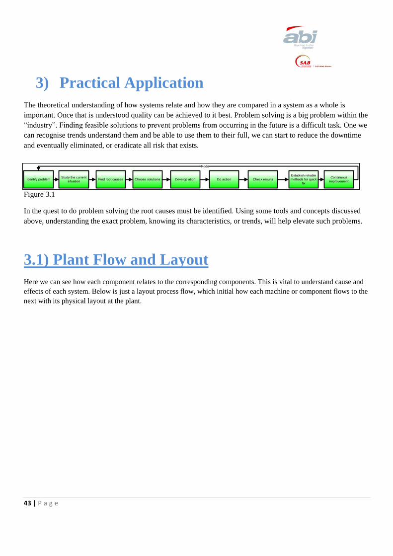
43 | P a g e

3) Practical Application

The theoretical understanding of how systems relate and how they are compared in a system as a whole is

important. Once that is understood quality can be achieved to it best. Problem solving is a big problem within the

“industry”. Finding feasible solutions to prevent problems from occurring in the future is a difficult task. One we

can recognise trends understand them and be able to use them to their full, we can start to reduce the downtime

and eventually eliminated, or eradicate all risk that exists.

Figure 3.1

In the quest to do problem solving the root causes must be identified. Using some tools and concepts discussed

above, understanding the exact problem, knowing its characteristics, or trends, will help elevate such problems.

3.1) Plant Flow and Layout

Here we can see how each component relates to the corresponding components. This is vital to understand cause and

effects of each system. Below is just a layout process flow, which initial how each machine or component flows to the

next with its physical layout at the plant.

Identify problemStudy the current

situationFind root causes Choose solutions Develop ation Do action Check results

Establish reliable

methods for quick

fix

Continuous

improvement

Redo

44 | P a g e

3.1.1) Water Treatment plant

Raw water Treated water

500kL 500kL

P Q

Softener

Softener

Soft

storage

Cl

dosse

r

Carbon

Filer 1

Carbon

Filer 2

Carbon

Filer 3

UV PF 3

Cl

dosse

r

PF 2

PF 1

Nano 1

Nano 2

Nano 3

Line 1

Line 2

Syrup

Line 3

P

Boiler

Line 2 B/W

Line 1 B/W

Figure 3.1.1

45 | P a g e

3.1.2) Ammonia Plant

Condensers

NH3

Unisab II

Comp 2

Unisab III

Comp 3

Unisab II

Comp 1

Liquid Receiver

Heat

Exchanger

Heat

Exchanger

NH3

Supply to line

Chilled

water

tank

Water

Figure 3.1.2

46 | P a g e

3.1.3) Compressor plant

3.1.3.1) 40 bar

Comp Mid Comp Air

Water flow

Water flow

Line 3

Comp air

Figure 3.1.3.1

47 | P a g e

3.1.3.2) 7 bar

Air

Dryer 1

IR 7 Bar

compressor

Atlas Copco 7 Bar

compressor

Comp Air 7 Bar

compressor

Air

receiver

Air

Dryer 2

Plant

90 kW

90 kW

Figure 3.1.3.2

48 | P a g e

3.1.4) CO2 Plant

CO2

Tank 1

CO2

Tank 2

Regulator

Line 3

Line 1

CO2

Tank 5

CO2

Tank 4

CO2

Tank 3

CO2

Tank 6

25T ABI 26T ABI

18T Afrox 18T Afrox

Line 2

This flow meter must

balance with usage at lines

Pressure

Flow (kg/hr)

Pressure

Flow (kg/hr)

Pressure

Flow (kg/hr)

???

Figure 3.1.4

49 | P a g e

3.1.5) Boiler room

Boiler 1 Boiler 2

Water treatment plant

Bottle washer 1

Bottle washer 2

Syrup room

Hot

Well

5TPH

10 Bar

5TPH

10 Bar

Softners

Pressure

Temp

Figure 3.1.5

50 | P a g e

3.2) Finding problems

Here we see downtime affecting the plant over the last year. Looking at the first histogram the total downtime

occurred versus other non production events is illustrated. It can be seen that allowed stoppages and maintenance

has the same duration in production failure as downtime. This should not be the case as maintenance should

prevent and eliminate all downtime occurred.

Table 3.2.1

Using histogram 2 it is easy to see in which months and weeks where the most down time occurred but it is also

very helpful to see in which area that down time did occur. Here in the early part of the year refrigeration cause a

large amount of downtime, followed the CO2 plant.

0.083641434

0.243196251

0.082294791 0.093984102

0.0453774960.05872434

0.338885253

0.078584248 0.091255290.064098818

0.101119824

0.282083407

0.086596326 0.0862098690.116388435

0.175461276

0.118227759 0.103419908 0.1018921140.070043483

00.05

0.10.15

0.20.25

0.30.35

0.4

Downtime Adjustments Maintenance & cleaning

Allowed stoppages

Service stoppages

Downtime Loss Categories

52 Weeks 13 Weeks4 Weeks Week 37

51 | P a g e

.

Table 3.2.2

Overlooking over the last financial year to date the trend within downtime attained at Devland. The trend shows

an uncontrolled system where one week the % of downtime occurs is low to that of the following week to be one

of the highest. This system is shown to be out of control. This chaotic system needs to be neutralized and

“tamed” to a manageable state where nothing is unpredictable.

0.00%

0.50%

1.00%

1.50%

2.00%

2.50%

Total F08

Total F09

Total F10

April May Jun Jul Aug Sep Oct Nov Dec Jan Feb Mar YTD

% o

f A

FH

Devland - Utilities Downtime F11

Elect Water Water Treat Steam

Refridge CO2 Air HP Air LP

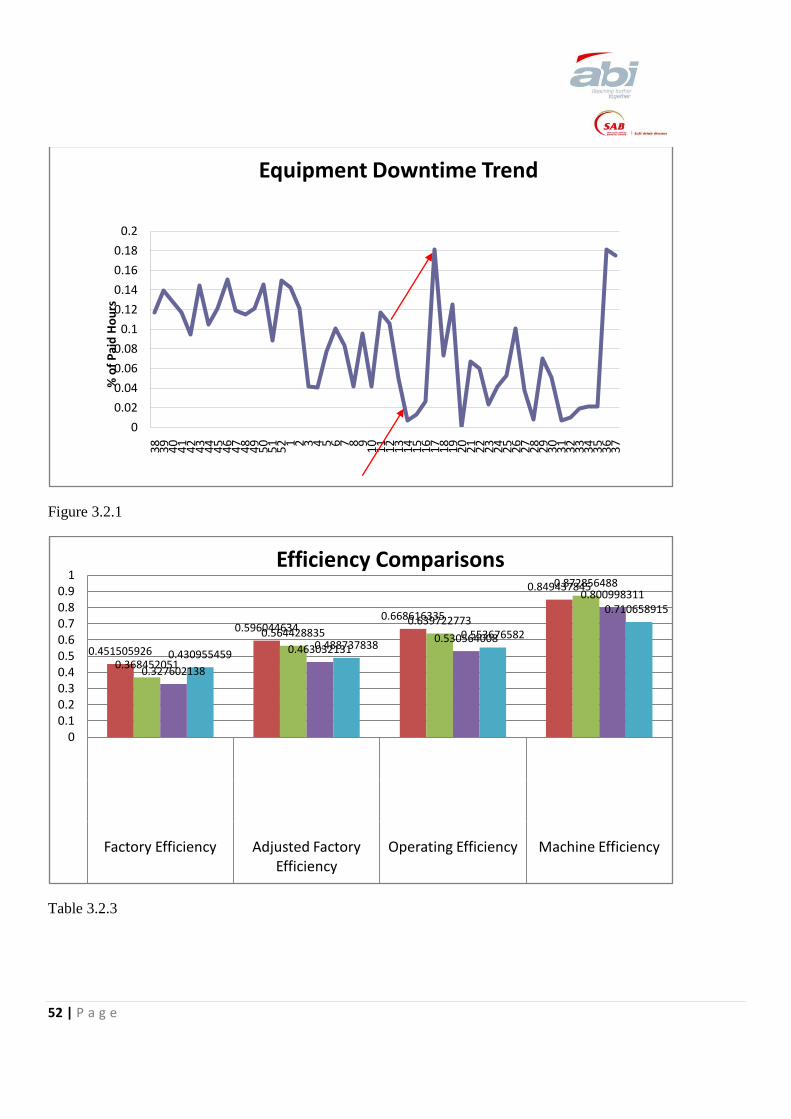
52 | P a g e

Figure 3.2.1

Table 3.2.3

0

0.02

0.04

0.06

0.08

0.1

0.12

0.14

0.16

0.18

0.2

38

39

40

41

42

43

44

45

46

47

48

49

50

51

52 1 2 3 4 5 6 7 8 9

10

11

12

13

14

15

16

17

18

19

20

21

22

23

24

25

26

27

28

29

30

31

32

33

34

35

36

37

% o

f P

aid

Ho

urs

Equipment Downtime Trend

0.451505926

0.5960446340.668616335

0.849437845

0.368452051

0.5644288350.639722773

0.872856488

0.327602138

0.4630321310.530564008

0.800998311

0.4309554590.488737838

0.553676582

0.710658915

00.10.20.30.40.50.60.70.80.9

1

Factory Efficiency Adjusted Factory Efficiency

Operating Efficiency Machine Efficiency

Efficiency Comparisons

53 | P a g e

3.2.1) Understanding and interpreting control chart patterns

3.2.1.1) Problem 1:Cooling Tower Temperature

Once one has controlled the chart it should exhibit natural characteristics. These trends and patterns can be

analysed interoperated and feasible effective solutions can be brought up with the aid of other quality control

tools.

We can view on case below where temperature of the final product tended to be an issue in the production. The

ammonia plant cools the water to the desired temperature through heat exchanges.

Figure 3.2.1.1

Looking at the trending on the 6th of September one can see various patterns within the input of temperature of a

particular cooling tower. Prior to the red line one can see a sudden drop before a more cataclysmic temperature

declines. Even before that sudden drop one can see that the mean of the graph is below that of the standardised

average. A continual lower or lowering of the graph can show as an early indication for something that could, or

will occur. The time period for the plant to run according to its standard operating procedures is that of between

the red line and the blue line, which is a total of 18minutes. The problem that occurred is only 6 minutes long but

its trending patterns could be identified prior to its occurrence. These 6minutes resulted in a total of 18minutes of

production downtime. Further investigation must now be done to determine for the occurrence of this drop, and

as one comes more familiar with the trends one can use this to predict a possible downtime.

When the run chart has a sudden drop like this, it is imperative that the temperature is increased back to its norm.

This sudden drop can be used as an alarm to ensure the correct temperature is maintained.

Looking as a cause and effect diagram the reason for having a low temperature in the cooling tower going in

could be as a result of the chilled ammonia not having enough contact time with the chilled water, and if one

looks at the output of the chilled water we can see if that is the case, and one can act accordingly. One can then

reduce the flow rate of the ammonia to increase the contact time, or one can increase the temperature of the

ammonia of the water is at a standardised temperature. This will result in less work done in the refrigeration

cycle as having less stress on the ammonia compressors and the refrigeration system reducing the cost of

electricity and the maintenance due to higher than required operating procedures.

54 | P a g e

Refrigeration cycle of ammonia.

Figure 3.2.1.2

If one reduces the distance from point 1-2 then less work in needed to be performed for the cycle.(Work is

measured by the area of the block in the graph.) This results in having a higher evaporator pressure. As

temperature and pressure are proportional on must determine whether this compromise of work is ethical due to

the increase of both the characteristics (pressure and temperature) in the evaporator. Will this increase in

properties have a higher maintenance procedure and is it more prone to failure? All these cause and effects must

be analysed in detail considering all aspects to see where minimal stresses within the entire system can be

introduced, to have a more efficient quality driven productive process. Process team is then to decide according

to the evaporators running parameters and design specifications whether it can perform elevated parameters.

55 | P a g e

3.2.1.2) Problem 2: Low Treated Water

The water treatment is considered to have a low water level when the treated water tank, water after the Nano

membrane filters, is at a 40% value. The plant has an automatic shut down when the tank levels get below 30%.

Each Nano membrane produces 50m3 of usable treated water.

Understanding the flow of how water gets treated is vital to knowing how to solve a problem in the system. The

municipal water gets pumped to a raw water tank where some chlorine is dossed into the water. This Chlorine

changes the pH of the water accordingly. The water then flows from the raw water tan through the carbon filters

where the bacteria and germs are removed with the Chlorine. The water is then pushed through two polishing

filters one with 4 material bags, and another with one stainless steel micro filter. Thereafter the water is pump

through a suction pump to 3 delivery pumps where each of those pumps deliver water to the Nano membranes to

further filter the water. This is then sent to the treated water tank to be stored for the line to use. Once the line

requires water it is pumped through a final polishing filter and then treated with a UV sanitizer to kill the last

remaining micro organisms. Then the water is received to the in or syrup room where the treated water is

required. See Water treatment plant Flow diagram for clarification.

Here observation of run charts will be done.

Figure 3.2.1.2.1

In this we can see that the treated water level drops to a value of 31%. For manufacturing purposes the cut off

line for the pumps to automatically stop is at 30%. This is in place as to notify production that the water level is

too low, and something is wrong in the production of treated water. This occurred 3 times within the period of a

day. Just by this trend we can I identify a pattern that it should occur again. If it does it could possibly result in

the plant shutting down and occurring unnecessary downtime.

56 | P a g e

Figure 3.2.1.2.2

In the next figure it shows that the problem occurred at 01:26 am and was corrected the final time at 21:56 in the

evening of the same day. Often these problems are not noticed as no management or utilities staff members are

present at these times of the day. The identifying of why such a problem occurred is vital to resolving this

problem.

57 | P a g e

Figure 3.2.1.2.3

Here the flow rate from the Nano membranes are plotted showing the time they had flow through them and the

time they were off. The production of treated water was prevalent prior to 3:57am then switched off and never

came back on. The problem existed for a period of 1 hour and 17minutes and then resolved at a point where

production suffered a problem of downtime. Nano 3 was on then for some reason unknown went offline along

with the other Nano‟s. Normally the 2nd Nano would come on when the level is below 70% and the 3rd Nano at

50%. This did not occur as one can see. This means that for some reason the Nano‟s were forcefully put off. This

could be due to a downstream problem. The Nanos require pressure of 5bar-8bar to run. To little pressure results

in not enough force to go through the Nano‟s and too much pressure results in the destruction, or depreciation of

quality of the Nano membranes.

58 | P a g e

Figure 3.2.1.2.4

Here just the Nano 3 is inspected to see a relation as to why the Nano may have been switched off but never

returned back on.

59 | P a g e

Figure 3.2.1.2.5

Here the problem is focused to the time of 9:54 and 14:53. The problem is the similar as that which occurred in

the 1st observation, that the Nano‟s only come back on after it is too late.

Figure 3.2.1.2.6

60 | P a g e

The inspection of Nano 2 can be see that as soon as it comes back on the treated water level starts to incline.

Figure 3.2.1.2.7

The same observation is noticed for Nano 3

61 | P a g e

Figure 3.2.1.2.8

To see whether there is a lack of water supply from the initial source, the municipal feed, the raw water tank is

inspected at that time period. Here it is seen that the trend of the sudden depreciation in value for the treated

water is not affected from the possible shortage supply of raw water. The percentage of raw water in the raw

water tank is constant, and can see that in fact it does not fluctuate as the problem is upstream. With this it is

visible that there is an error between that of the treated water and the raw water buffer tanks. The problem occurs

again at a later stage.

62 | P a g e

Figure 3.2.1.2.9

Here we just looking at the problem discussed above with the raw water versus the treated water in a closer view.

Through this observation we can see the problem exists somewhere between the Carbon filter and before the

Nano‟s. Reference to the PIM‟s and POM‟s were used to identify where a problem may lie. Inspecting the PIM‟s

and POM‟s seen in Appendix Table 1. If we see the conductivity of the Nano membranes is less than 200µS,

which means the Nanos need to be cleaned. The PIM‟s and POM‟s showed a low in feed pressure value of 1.5

bar to the Nano‟s. Using the PIM‟s and POM‟s it is seen that the differential pressure between that of the

Polishing Filters one and two near 5bar which results in the filter bags needing replacement. Therefore there is a

blockage between the filters, due to the filter bags being blocked. The filter bags were replaced before they could

be completely blocked and cause longer downtime in production. Picking up this trend of a sudden decline will

eradicate the downtime that is the indication that the filter bags need replacement.

If we use 500 data point over a full day period the X R chart will be seen as.

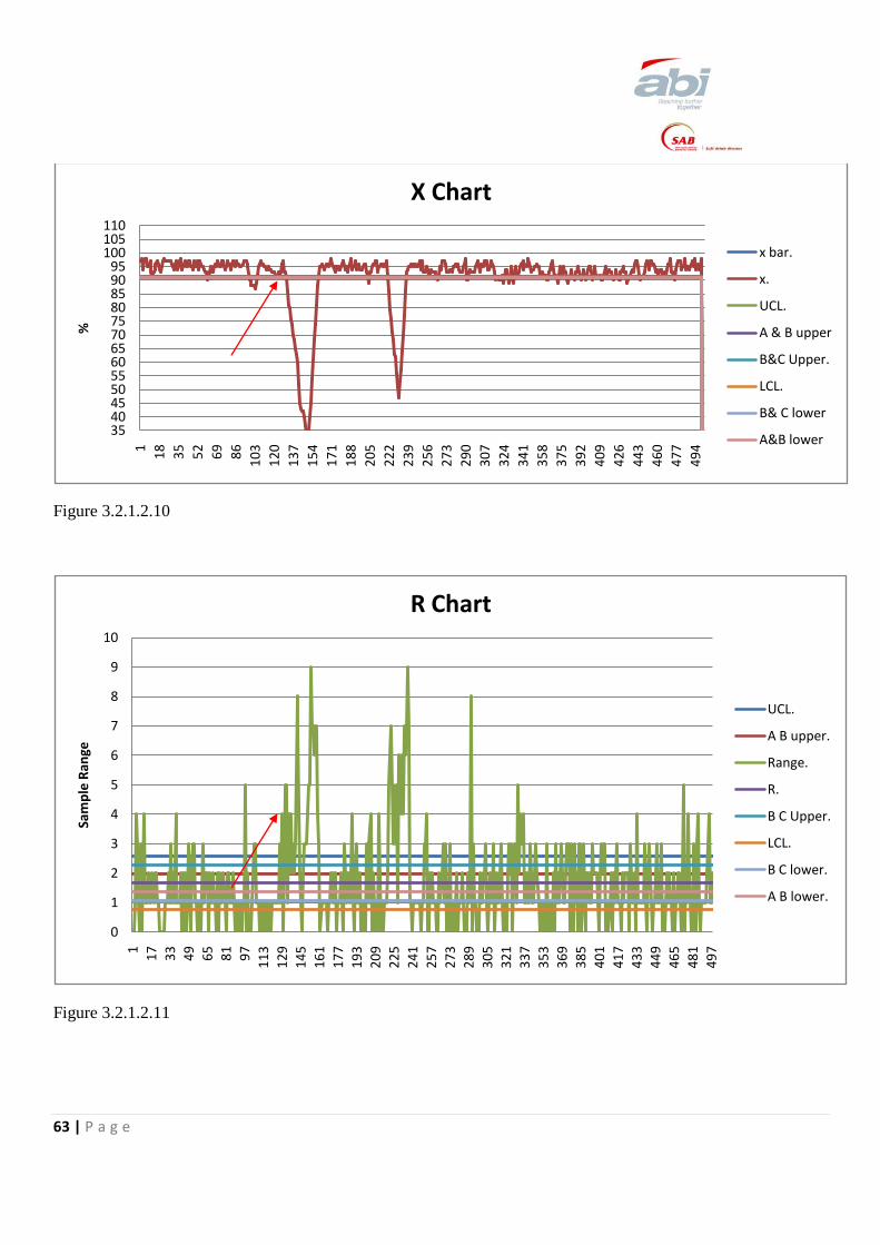
63 | P a g e

Figure 3.2.1.2.10

Figure 3.2.1.2.11

35404550556065707580859095

100105110

1

18

35

52

69

86

10

3

12

0

13

7

15

4

17

1

18

8

20

5

22

2

23

9

25

6

27

3

29

0

30

7

32

4

34

1

35

8

37

5

39

2

40

9

42

6

44

3

46

0

47

7

49

4

%

X Chart

x bar.

x.

UCL.

A & B upper

B&C Upper.

LCL.

B& C lower

A&B lower

0

1

2

3

4

5

6

7

8

9

10

1

17

33

49

65

81

97

11

3

12

9

14

5

16

1

17

7

19

3

20

9

22

5

24

1

25

7

27

3

28

9

30

5

32

1

33

7

35

3

36

9

38

5

40

1

41

7

43

3

44

9

46

5

48

1

49

7

Sam

ple

Ran

ge

R Chart

UCL.

A B upper.

Range.

R.

B C Upper.

LCL.

B C lower.

A B lower.

64 | P a g e

Here we can see that the R chart is completely out of statistical control. Another alarm to be triggered would be

when the process variance is larger than 4%. Even though the Upper control Limit is 3%, it can be deduced in

this situation and others like this that there will tend to be an error when there is a range of 4% or greater. It can

be seen when this 4% or greater error occurs this is when the large depreciation of water % in the tank occurs

from the X chart.

In working with the charts the capability of the chart needs to be determined.

Figure 3.2.1.2.12

Process capability

Cpl 0.200481

Cpu 0.200481

Cpk 0.200481

Table 3.2.1.2.1

Using the trends to identify that a problem such as this occurs can be used. Alarms should be implemented as

soon as the trend of the treated water depreciates to at a level lower than it can feed in over a period of time. If

such a trend exist of depreciating water level exists over a time period of 30min this will be an alarm that

something has gone wrong, in this case the polishing filters were blocked.

0

10

20

30

40

50

60

70

80

90

100

31

35

40

43

47

52

54

57

61

63

65

70

74

77

80

86

88

90

92

94

96

98

Process capability

65 | P a g e

3.2.1.3) Problem 3: CO2 Shortage

CO2 wastage tends to be a problem within production at ABI Devland. For every 1HL of water used in

production 1ton of CO2 is used. There is a tolerance of 25% of allowed wastage during production. The current

value of wastage at Devland is up to over 40% for the last four months. The issue is that the monetary value of

the CO2 is not of a large value, but the problem occurs that there is a shortage of CO2 supply country wide. The

problem is no matter how much money ABI wastes in CO2 losses it cannot be rebated through an actual CO2

loss. If there is no CO2 for the soft drinks there cannot be any production. This insufficient supply of CO2 results

in long durations of unnecessary downtimes.

To see where there are ways to save CO2 losses we need to understand the operation of the CO2 plant. Below is

a flow diagram of the flow chart from the CO2 storage tanks to the starblender where the CO2 is actually mixed,

in a particular ratio in accordance to a particular recipe for a particular product.

Figure 3.2.1.3.1

The CO2 pressure controls on the tanks are made up of two independent systems. The refrigeration unit is meant

to bring the pressure down if too high. The refrigeration unit brings the pressure down from 20 Bars and releases

it off at 18 bars. The evaporation unit is meant to increase pressure when too low. Then the evaporation unit

comes on at 15 Bar and releases pressure off at 17 Bar. The storage tanks mechanical safety blow off valves are

actuated at 23 Bar. The filler lines are rated at:

Line 1 600kg/hr at a maximum pressure of 20.7bar.

Line 2 2300kg/hr at a maximum pressure of 20.7 bar.

66 | P a g e

Potential places for CO2 losses.

Incorrect data capturing.

Incorrect pressure control at CO2 tanks.

Leakages from supply lines to filler.

Incorrect operation of the filler bowl pressures.

Incorrect capture of variance of actual usages by production line teams.

Modifications to the “On Line Filtration System”

To find if there were losses all handling points need to be inspected and verified that no losses occur in their

subsystems. All deliveries to site from Afrox were checked and verified that all receipts were correctly captured.

The Star Blenders also have potential losses; alarms were often low pressure alarms, showing that there tends to

be a problem upstream. There tended to be a variance in actual usage by the filler versus volume based usage.

The inspections of the CO2 lines, from the tanks to the production lines, were done to verify that no leaks occur

within the system. There were small leaks at the CO2 tanks and in the lines in which the CO2 run through. These

leaks were corrected and sealed. There tended to be excessive blow offs of releasing pressure between

subsystems to elevate excess pressure within that particular subsystem.

Attempts to reduce the maximum pressure supplied to the filter have proved unsuccessful as it brings the

refrigeration unit to operate between 17 – 19 bars we need to bring down the evaporation unit to operate at 14 -

16 bars. The regulating valve works on differential pressure. When pressure rises to 23 bar need to reduce it by 2

bars to below 21 bars, and when pressure drops to 14 bars regulator will drop it to 12 bars. The Star blender CO 2

injector requires a minimum of 15 bars to operate. The new advised operating range is to operate from a range of

15-23bar to a range of 15-21bar

Other recommendations are that if long breakdowns or long shut downs, due to maintenance, do occur the

production lines need to switch off the feed of the CO2 to the line to ensure no losses further downstream.

67 | P a g e

3.2.1.4) Problem: Sugar Brix

In order for the line to receive the correct quantity of sugar mixed with water, (simple syrup) used in the

production of the concentrate, the plant needs to be confident that it will attain a Brix value (sugar water mixture

value) of 62º Brix.

Overlooking just a few days to see whether the plant in fact does have the confidence it requires to product this

Brix. Figure 3.1 we can see that the Brix value frequently changes and needs to be monitored on a regular basis.

If there are any sudden drops such as indicated in the figure alarms need to be triggered to prevent the line from

receiving inadequate quality of Brix. By looking at this graph once this problem occurs it follows a pattern where

it continues over a period to suddenly drop in Brix.

Figure 3.2.1.4.1

68 | P a g e

In the X and S chart the trends are identified over a period of 4 days. Every period runs over one full production

shift, 7:00am to 4:00pm. 500 intervals are taken per sub section to insure accurate evaluation. With this every

64,8 seconds a new reading is taken place. By the 375th reading or at 13:45 there tend to be a regular increase in

excess Brix. When this Patten is identified X chart and the S chart simultaneously increase there is a over dosing

of sugar into the continuous sugar dissolver.

Figure 3.2.1.4.2

56

57

58

59

60

61

62

63

64

65

66

1

22

43

64

85

10

6

12

7

14

8

16

9

19

0

21

1

23

2

25

3

27

4

29

5

31

6

33

7

35

8

37

9

40

0

42

1

44

2

46

3

48

4

Bri

x V

alu

e

X Chart

xbar.

xdbar.

A & B upper.

LCL.

B & C lower.

B & C Upper.

A & B lower.

UCL.

69 | P a g e

Figure 3.2.1.4.3

0

1

2

3

4

5

6

7

8

1

21

41

61

81

10

1

12

1

14

1

16

1

18

1

20

1

22

1

24

1

26

1

28

1

30

1

32

1

34

1

36

1

38

1

40

1

42

1

44

1

46

1

48

1

(bla

nk)

Stan

dar

d d

evi

atio

n

S Chart

s.

Sbar.

LCL.

A & B lower.

B & C Upper.

A & B upper.

B & C lower.

UCL.

70 | P a g e

3.2.1.5) Problem 5: Sugar silo

A typical display of the consumption of sugar usage versus sugar loading is at “play” in this diagram. As the one

silo increases in volume, the other decreases in volume. The aim of the silo is to ensure that the sugar usage

never exceeds the sugar loading when the quantity of sugar at hand is below a particular point. A As long as there

is a continual sugar supply ability for the production team there should be no downtimes occurred in this

constraint.

Figure 3.2.1.5.1

Consumed

Loaded

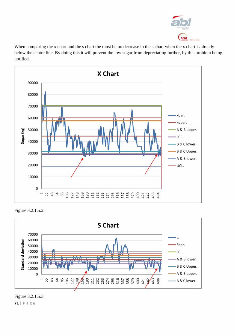
71 | P a g e

When comparing the x chart and the s chart the must be no decrease in the s chart when the x chart is already

below the centre line. By doing this it will prevent the low sugar from depreciating further, by this problem being

notified.

Figure 3.2.1.5.2

Figure 3.2.1.5.3

0

10000

20000

30000

40000

50000

60000

70000

80000

90000

1

22

43

64

85

10

6

12

7

14

8

16

9

19

0

21

1

23

2

25

3

27

4

29

5

31

6

33

7

35

8

37

9

40

0

42

1

44

2

46

3

48

4

Suga

r (k

g)

X Chart

xbar.

xdbar.

A & B upper.

LCL.

B & C lower.

B & C Upper.

A & B lower.

UCL.

0

10000

20000

30000

40000

50000

60000

70000

1

22

43

64

85

10

6

12

7

14

8

16

9

19

0

21

1

23

2

25

3

27

4

29

5

31

6

33

7

35

8

37

9

40

0

42

1

44

2

46

3

48

4

Stan

dar

d d

evi

atio

n

S Chart

s.

Sbar.

LCL.

A & B lower.

B & C Upper.

A & B upper.

B & C lower.

72 | P a g e

When the problem, as indicated by the red arrows, occurs where there is more going out of the silos than being

fed into the silos, the total sugar is below the lower control limit between the lower B and C line notification

needs to be done, to prevent more loss of sugar from accruing. Having too much sugar, in this case, is not an

issue.

73 | P a g e

3.2.1.5) Problem 5: Nano membranes

Earlier the level of treated water was under scope, problem solving and other issues were addressed. In this case

the Nano membranes failed to perform at its standard operating parameters. If one observes the standard Nano

flow rate, one will see that it is either on or off, and when on it has a flow rate of 50m3/hr. An alarm for this case

must be triggered when the plant cannot function to its required specification.

Figure 3.2.1.6.1

In this figure, as indicated, it is already raised that there must be a trigger, and alarm for when the treated water is

below a level of 40% to prevent production from stopping. This is not where the issue in this case lies.

74 | P a g e

Figure 3.2.1.6.2

One can see that the Nano is running to its standard operating procedures at 50m3/hr, when there seems to be a

spike in both the Nano flow rate and the treated water level. Here after the Nano continues to operatate at 50% its

normal operation, 25m3/hr.

75 | P a g e

Figure 3.2.1.6.3

This figure just shows the Nano flow rate individually.

76 | P a g e

Figure 3.2.1.6.4

The treated water level is compared to that of the raw water level and it can be seen that the raw water level is

chaotically out of control. The data points fluctuate from one point to the next. The plant is then shut down as no

production was scheduled for the Sunday evening. This allowed the plant to “relax and readjust the levels and

flows.

77 | P a g e

Figure 3.2.1.6.5

This is just a visual of all the Nanos flow rates along with the raw water and the treated water levels.

One can conclude that if the Nanos operate at a 50% functionality, or 25m3/hr, the plant needs to reset following

the standard shut down and start up procedures.

78 | P a g e

79 | P a g e

4) Conclusion

In this project on can see how analysing raw data can influence and aid in the prevention of downtime within a

manufacturing company. There are various ways in which to help prevent curtain circumstances, but the real problem

is that they are all individual and are isolated to certain circumstances. One of the biggest problems in engineering is

not really the problem, of how to fix a problem, but what is the problem. The aid of such a project is not to help solve

on isolated event or problem, but it allows for constant continual improvement within a system by being able to

understand a problem. By understanding a particular problem and finding where an error exists solving the situation

could not be too hard. Often in a place where know one understand what when wrong there cannot be a feasible

solution as the problem addressed it not know. By using the tools identified we can see that there are various situations

that could arise, but if one follows certain procedures to mitigate errors these errors over time will diminish, and in an

ideal state seize to exist. The problem is that each error is unique to the situation in which it is addressed, but knowing

what to look for in characteristics, trends, patterns, and anything that really just sticks out from an ordinary state, will

help aid in the start to resolving a problem. For such trends and errors that occur within the plant “quick fix”

procedures need to be implemented. There are various issues that could result in various problems. The hardest part is

being able to resolve issues effortlessly and without any concern. (See quick fix procedures for water treatment plant

in appendix). As the understandings of these trends begin to be identified before the problems occur, a solution to this

can be implemented and all issues resolved.

A real problem faced in the engineering field is that many engineers find a problem but they are not too sure how the

system works, and they try to find an ideal solution. In many ways that ideal solution is not ideal and in fact is not the

root cause of an error.

These problems could continue from isolated event to regular frequent events, but the use of such a project is to be

able to identify an error within the system as a whole find the roots error and resolve it in the most suitable way. May

this solution be changing a filter bag, or undergoing a production standard, or redesigning the subsystem to aid in the

efficiency of the system as a whole, or not needing a solution at all as the problem was an isolated “freak” error?

80 | P a g e

81 | P a g e

5) Appendices In designing the PIM‟s and POM‟s for the check sheet used in the study, certain factors had to be known. The standard

operation parameters and the design parameters. The plants in the water treatment and the utilities department have

known operation procedures. Without certain parameters met the plant is unable to perform at its desired

specifications. Other characteristics are not part of design specifications and need to be adjusted once a known

parameter is deduced from studies. These factors are standard operating temperatures, pressures electric flow rates,

speeds and other measurable parameters.

5.1) PIM‟s and POM‟s water treatment Plant

Process Artisan: Controller:

Date:

Daily Units Min Max OK OK OK OK OK OK OK

Municipal flow Pressure kPa kPa kPa O.K. kPa O.K. kPa O.K. kPa O.K. kPa O.K. kPa O.K. kPa O.K.

500kL tank Level 75% 100% % O.K. % O.K. % O.K. % O.K. % O.K. % O.K. % O.K.

Level 50% 100% % O.K. % O.K. % O.K. % O.K. % O.K. % O.K. % O.K.

Pressure Line 1 kPa kPa kPa O.K. kPa O.K. kPa O.K. kPa O.K. kPa O.K. kPa O.K. kPa O.K.

Pressure Line 2 kPa kPa kPa O.K. kPa O.K. kPa O.K. kPa O.K. kPa O.K. kPa O.K. kPa O.K.

Chlorine Dosing tank Level 30% 100% % O.K. % O.K. % O.K. % O.K. % O.K. % O.K. % O.K.

Chlorine correction tank Level 100L 250L L O.K. L O.K. L O.K. L O.K. L O.K. L O.K. L O.K.

Anti-scalent tank Level 50L 120L L O.K. L O.K. L O.K. L O.K. L O.K. L O.K. L O.K.

Level 75% 100% % O.K. % O.K. % O.K. % O.K. % O.K. % O.K. % O.K.

Pressure pump 1 kPa kPa kPa O.K. kPa O.K. kPa O.K. kPa O.K. kPa O.K. kPa O.K. kPa O.K.

Pressure Pump 2 kPa kPa kPa O.K. kPa O.K. kPa O.K. kPa O.K. kPa O.K. kPa O.K. kPa O.K.

Level 75% 100% % O.K. % O.K. % O.K. % O.K. % O.K. % O.K. % O.K.

Pressure pump 1 kPa kPa kPa O.K. kPa O.K. kPa O.K. kPa O.K. kPa O.K. kPa O.K. kPa O.K.

Pressure Pump 2 kPa kPa kPa O.K. kPa O.K. kPa O.K. kPa O.K. kPa O.K. kPa O.K. kPa O.K.

Δ Pressure kPa 100kPa kPa O.K. kPa O.K. kPa O.K. kPa O.K. kPa O.K. kPa O.K. kPa O.K.

Temperature in °C °C °C O.K. °C O.K. °C O.K. °C O.K. °C O.K. °C O.K. °C O.K.

Δ Pressure kPa 100kPa kPa O.K. kPa O.K. kPa O.K. kPa O.K. kPa O.K. kPa O.K. kPa O.K.

Temperature in °C °C °C O.K. °C O.K. °C O.K. °C O.K. °C O.K. °C O.K. °C O.K.

Δ Pressure kPa 100kPa kPa O.K. kPa O.K. kPa O.K. kPa O.K. kPa O.K. kPa O.K. kPa O.K.

Temperature in °C °C °C O.K. °C O.K. °C O.K. °C O.K. °C O.K. °C O.K. °C O.K.

Chlorine 5ppm 8ppm ppm O.K. ppm O.K. ppm O.K. ppm O.K. ppm O.K. ppm O.K. ppm O.K.

Turbidity NTU O.K. NTU O.K. NTU O.K. NTU O.K. NTU O.K. NTU O.K. NTU O.K.

Polishing filters 1 and 2 Δ Pressure kPa kPa O.K. kPa O.K. kPa O.K. kPa O.K. kPa O.K. kPa O.K. kPa O.K.

Post Polishing filter Chlorine 0ppm ppm O.K. ppm O.K. ppm O.K. ppm O.K. ppm O.K. ppm O.K. ppm O.K.

Main Nano flow in Pressure 1.5bar 5bar bar O.K. bar O.K. bar O.K. bar O.K. bar O.K. bar O.K. bar O.K.

Pressure in 8bar bar O.K. bar O.K. bar O.K. bar O.K. bar O.K. bar O.K. bar O.K.

Conductivity 200μS/cm μS/cm O.K. μS/cm O.K. μS/cm O.K. μS/cm O.K. μS/cm O.K. μS/cm O.K. μS/cm O.K.

Flow rate 0m3/hr 50m3/hr m3/hr O.K. m3/hr O.K. m3/hr O.K. m3/hr O.K. m3/hr O.K. m3/hr O.K. m3/hr O.K.

Pressure in 8bar bar O.K. bar O.K. bar O.K. bar O.K. bar O.K. bar O.K. bar O.K.

Conductivity 200μS/cm μS/cm O.K. μS/cm O.K. μS/cm O.K. μS/cm O.K. μS/cm O.K. μS/cm O.K. μS/cm O.K.

Flow rate 0m3/hr 50m3/hr m3/hr O.K. m3/hr O.K. m3/hr O.K. m3/hr O.K. m3/hr O.K. m3/hr O.K. m3/hr O.K.

Pressure in 8bar bar O.K. bar O.K. bar O.K. bar O.K. bar O.K. bar O.K. bar O.K.

Conductivity μS/cm200μS/cm μS/cm O.K. μS/cm O.K. μS/cm O.K. μS/cm O.K. μS/cm O.K. μS/cm O.K. μS/cm O.K.

Flow rate 0m3/hr 50m3/hr m3/hr O.K. m3/hr O.K. m3/hr O.K. m3/hr O.K. m3/hr O.K. m3/hr O.K. m3/hr O.K.

Nano CIP required? Check Yes/No O.K. Yes/No O.K. Yes/No O.K. Yes/No O.K. Yes/No O.K. Yes/No O.K. Yes/No O.K.

Conductivity post nano Micro Siemens 200μS/cm μS/cm O.K. μS/cm O.K. μS/cm O.K. μS/cm O.K. μS/cm O.K. μS/cm O.K. μS/cm O.K.

Intensity W/cm2 O.K. W/cm4 O.K. W/cm6 O.K. W/cm8 O.K. W/cm9 O.K. W/cm11 O.K. W/cm12 O.K.

Lamp 1 current 9.5 A A O.K. A O.K. A O.K. A O.K. A O.K. A O.K. A O.K.

Lamp 2 current 9.5 A A O.K. A O.K. A O.K. A O.K. A O.K. A O.K. A O.K.

Lamp 3 current 9.5 A A O.K. A O.K. A O.K. A O.K. A O.K. A O.K. A O.K.

Lamp 4 current 9.5 A A O.K. A O.K. A O.K. A O.K. A O.K. A O.K. A O.K.

UV Dose 40mJ/cm2250mJ/cm2 mJ/cm2 O.K. mJ/cm4 O.K. mJ/cm6 O.K. mJ/cm8 O.K. mJ/cm9 O.K.mJ/cm11 O.K.mJ/cm12 O.K.

hours 4000hr hr O.K. hr O.K. hr O.K. hr O.K. hr O.K. hr O.K. hr O.K.

Instrument air Pressure kPa kPa kPa O.K. kPa O.K. kPa O.K. kPa O.K. kPa O.K. kPa O.K. kPa O.K.

Alarms on PLC Check O.K. O.K. O.K. O.K. O.K. O.K. O.K.

Sign:

Comments:

01:00 03:0007:00 11:00 19:00 21:00

Process Artisan: Controller:

15:00

UV Sanitizer

Permeate Water

Pre Polishing filter

Nano 2

Water Treatment Plant Monitoring

Nano 3

Softened water

Carbon Filter 1

Carbon Filter 2

Carbon Filter 3

Nano 1

Raw tank

Table 5.1.

82 | P a g e

5.2) Different Control Charts

Chart type Process

Observation

type

X and R chart Quality characteristic within one subgroup Variable

X and S chart Quality characteristic within one subgroup Variable

Im R and XmR

chart Quality characteristic within one subgroup Variable

Three way chart Quality characteristic within one subgroup Variable

P chart Fraction nonconforming within one subgroup Attribute

np chart Number nonconforming within one subgroup Attribute

c chart Number of conformances within one subgroup Attribute

u chart Conformances per unit within one subgroup Attribute

EWMA chart

Exponentially weighted moving average of

quality characteristics measurement within one

subgroup

Attribute or

Variable

CUSUM chart

Cumulative sum of quality characteristic

measurement within one subgroup

Attribute or

Variable

Time series

model

Quality characteristic measurement within one

subgroup

Attribute or

Variable

Regression

control chart Quality characteristic within one subgroup Variable

Real time

contrast chart

Sliding window of quality characteristic

measurement within one subgroup

Attribute or

Variable

Table 5.2

83 | P a g e

5.3) Control Chart Constants

Table 5.3

Sample

Size =

n

A2 A3 d2 D3 D4 B3 B4

2 1.88 2.659 1.128 -- 3.267 -- 3.267

3 1.023 1.954 1.693 -- 2.574 -- 2.568

4 0.729 1.628 2.059 -- 2.282 -- 2.266

5 0.577 1.427 2.326 -- 2.114 -- 2.089

6 0.483 1.287 2.534 -- 2.004 0.03 1.97

7 0.419 1.182 2.704 0.076 1.924 0.118 1.882

8 0.373 1.099 2.847 0.136 1.864 0.185 1.815

9 0.337 1.032 2.97 0.184 1.816 0.239 1.761

10 0.308 0.975 3.078 0.223 1.777 0.284 1.716

11 0.285 0.927 3.173 0.256 1.744 0.321 1.679

12 0.266 0.886 3.258 0.283 1.717 0.354 1.646

13 0.249 0.85 3.336 0.307 1.693 0.382 1.618

14 0.235 0.817 3.407 0.328 1.672 0.406 1.594

15 0.223 0.789 3.472 0.347 1.653 0.428 1.572

16 0.212 0.763 3.532 0.363 1.637 0.448 1.552

17 0.203 0.739 3.588 0.378 1.622 0.466 1.534

18 0.194 0.718 3.64 0.391 1.608 0.482 1.518

19 0.187 0.698 3.689 0.403 1.597 0.497 1.503

20 0.18 0.68 3.735 0.415 1.585 0.51 1.49

21 0.173 0.663 3.778 0.425 1.575 0.523 1.477

22 0.167 0.647 3.819 0.434 1.566 0.534 1.466

23 0.162 0.633 3.858 0.443 1.557 0.545 1.455

24 0.157 0.619 3.895 0.451 1.548 0.555 1.445

25 0.153 0.606 3.931 0.459 1.541 0.565 1.435

84 | P a g e

5.4) Water treatment Plant Standard operating Procedures.

Process

Flow

m3/hr) Pressure (kPa)

Capacity

(m3) Quality/Chemicals/Time

Municipal Inlet Supply 180 <600

Liquid Chlorine Storage & Dosing (TK8/P8): 16 lph 500 500 liters

5-8ppm - 10 % Calcium

Hypochlorite

Raw Water Storage Tank TK1 73 Galv Sectional Steel

Raw Water Supply Pump (P1A/B): 160 400

Filtration Section:

Inlet Supply To Carbon Filters 160 400

Activated Carbon Filters (CF1A-C) 3 x 53 <600 Automated

Service/Rinse Flow Rate 53 8.8 Rinse 10 Minutes

Backwash Flow Rate 92 15.3 10 Minutes

Steaming 250 kg/hr 120 120 deg. C

Polishing Filters (PF1A/B) 1 x 160 <600 5 X 20 micron PP Bag

Polishing Filters (PF2A/B) 1 x 160 <600

16 X 5 micron 40”

Elements

Nano Feed Pumps (P5A/B/C): 3 x 61 560 One per Nano Skid

Membrane Section: Chemical Dosing:

Nano pH Correcting Storage & Dosing

(TK3/P3): 17 lph 400 250 liters 10 % Sulphuric Acid

Nano Anti-Scalent Storage &

Dosing(TK4/P4A/B/C): 3.9 lph 700 140 liters

2-3 ppm - 20 % MDC

200

Membrane Section: Nano 1/2/3

Feed Flow: 61.2 590 Including Recycle

Permeate Flow: 50 100

Recycle Flow: 6-7 280

Reject Flow: 4.4 280 92% Recovery

85 | P a g e

Stage 1 Permeate Backpressure 200 KPa

Stage 1

590 (inlet) 420

(outlet) 6 Housings

36 NF 270-400

Elements

Stage 2 :

420 (inlet) 280

(outlet) 3 Housings 18 NF 90-400 Elements

Treated Water Section:

Treated Water Storage (TK5): 60 304L SS

Treated Water Supply Pumps (P6A/B/C): 150-220 580 Cascade Duty

Aseptic Breather (VB1) 220 5 x Teflec Cartridges

Treated Water Section: Polishing, UV:

Polishing Bag Filter (PF3): 220 580

Ultra Violet Sterilization System (UV1): 150-220 600 Existing Unit

Treated Water return: 11

450 (min) 580

(max) SRV 01

General:

Plant Air Supply: 0.5 500-600 Oil Free

Table 5.4

86 | P a g e

5.5) Water treatment Plant Quick fix Procedures. FAULT PANEL

INDICATION &

ALARM

CHECK ACTION

Nano pH Low AT04 reads <6.5.

Alarm; Nano

Inlet pH low on

trending below

lower control

limit

Check pH monitor status. If monitor status is OK then check

dosing control & acid dosage from

P3.

Nano inlet Pressure Transmitter

(PT01/2/3) > 10,7 bar

Alarm; Nano

Inlet Pressure

High

Check Recycle & Reject flow

rates. Check permeate flow

rates.

If flow rates out of spec, adjust to

correct settings.

Nano inlet Pressure Switch (PS01)

< 1,0 bar

Alarm; Nano

Inlet Pressure

Low

Check if Carbon filters “On

line” and if Polishing filters are

clean differential pressure <

100 KPa.

Place Carbon Filters “On line” And

replace bags/cartridges is dirty.

Nano Permeate AT05/6/7

Conductivity reads > 200 uS/cm

Alarm; Nano

Permeate

Conductivity

High on trending

above upper

control limit.

Check Conductivity Monitor

status.

If monitor status is OK then check

treated water flow rate and inlet

pressure.

Nano Permeate Backpressure <1,8

bar or > 2,2 bar

Trend on water

treatment drops

slowly over

30min

Check Recycle & Reject low

rates. Check permeate flow

rates. Check backpressure

control valve RV3A/B/C.

If flow rates out of spec, adjust to

specification.

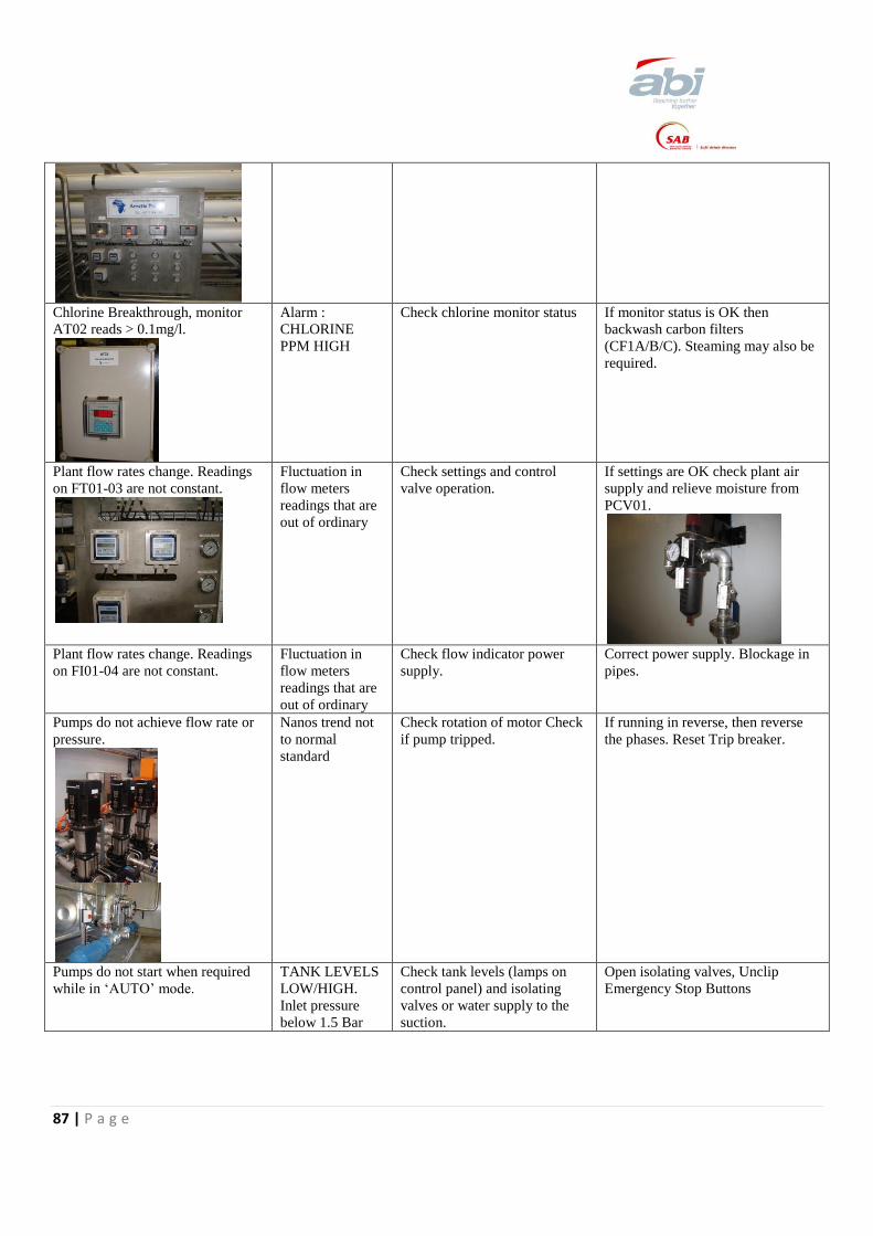
87 | P a g e

Chlorine Breakthrough, monitor

AT02 reads > 0.1mg/l.

Alarm :

CHLORINE

PPM HIGH

Check chlorine monitor status If monitor status is OK then

backwash carbon filters

(CF1A/B/C). Steaming may also be

required.

Plant flow rates change. Readings

on FT01-03 are not constant.

Fluctuation in

flow meters

readings that are

out of ordinary

Check settings and control

valve operation.

If settings are OK check plant air

supply and relieve moisture from

PCV01.

Plant flow rates change. Readings

on FI01-04 are not constant.

Fluctuation in

flow meters

readings that are

out of ordinary

Check flow indicator power

supply.

Correct power supply. Blockage in

pipes.

Pumps do not achieve flow rate or

pressure.

Nanos trend not

to normal

standard

Check rotation of motor Check

if pump tripped.

If running in reverse, then reverse

the phases. Reset Trip breaker.

Pumps do not start when required

while in „AUTO‟ mode.

TANK LEVELS

LOW/HIGH.

Inlet pressure

below 1.5 Bar

Check tank levels (lamps on

control panel) and isolating

valves or water supply to the

suction.

Open isolating valves, Unclip

Emergency Stop Buttons

88 | P a g e

Auto valves XVxx do not open.

No flow on Nano

Filters after

10min.

Check air supply and pressure Adjust air station PCV02 regulating

knob until gauge is 600kPa.

Table 5.5

89 | P a g e

6) Resources The following recourses were used:

W.E. Demings (1993) The new Economics for Industry, Goverment Education (Cambridge, MA:

Massachusetts Institute of Technology).

Deming, W E (1975) "On probability as a basis for action." The American Statistician. 29(4), p146–152

Deming, W E (1986) Out of the Crisis, (Cambridge, MA: Massachusetts Institute of Technology for

Advanced engineering study).

Ishikawa, Kaoru (1990), (Translator: J. H. Loftus), Introduction to Quality Control, p448

GITLOW HS, OPPENHEIM AJ, OPPENHEIM R & LEVINE DM, Quality Management,

Goldstine, Herman (1972). The Computer from Pascal to Von Neumann. Princeton University Press.

p266–267

Values can be found in the table B1. Based on that of ASTM Manual of Data and Control Chart Analysis

p134-136.

http://refrigerationblog.wordpress.com/author/artawina/

http://en.wikipedia.org/wiki/Control_chart

www.stat.ufl.edu/~kyung/sta3032/.../table_of_control_chart_constants.pdf

Warren Brussee,, “All about six sigma: the easy way to get started” , McGraw-Hill Professional (2005)

p237

Akao, Yoji. "Development History of Quality Function Deployment".

The Customer Driven Approach to Quality Planning and Deployment. Minato, Tokyo 107 Japan: Asian

Productivity Organization p339.

“Quality Management” 3rd Edition by McGraw Hill Figure 6.10 Chapter 6 page 163)

http://www.qualityamerica.com/knowledgecente/knowctrWhen_to_Use_an_Xbar_S_Chart.htm

The Journal of Quality Assurance Institute, Vol. 14, No. 1, January 2000, pp. 4-6 & 35-41.

Deming, W. Edwards, Lectures on statistical control of quality., Nippon Kagaku Gijutsu Remmei, 1950

Shewhart, W A (1939) “Statistical Method from the Viewpoint of Quality Control”

Shewhart, W A (1931) “Economic Control of Quality of Manufactured Product”

Imai. M. Kaizen, “The Key to Japan‟s Competitive Success”, New York City: Random House, 1986

King. B. Hoshin Planning, “The Developmental approach Methuen”, MA: Goal/ QPC, 1990, pg 1-13

Brussee Warren, “All About Six Sigma”, Mc-Graw-Hill 2006,. Pg21-27

Terry Bahill, „Systems engineering‟, 3rd edition, McGraw-Hill, 2005

//:beernet.com

90 | P a g e