brain-like design of sensory-motor programs for robots g. palm, uni-ulm
Post on 19-Dec-2015
213 views
TRANSCRIPT
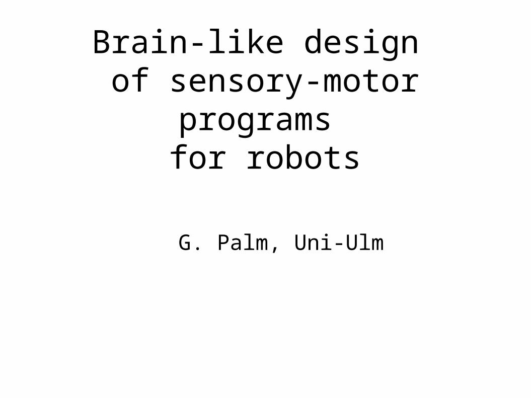
Brain-like design of sensory-motor programs
for robots
G. Palm, Uni-Ulm

The cerebral cortex is a huge associative memory,
or rather a large network of associatively connected topographical areas.
Associations between patterns are formed by Hebbian learning.
Even simple tasks require the interaction of many cortical areas.

Modelling Cortical Areas withAssociative Memories
Andreas Knoblauch & Günther PalmDepartment of Neural Information Processing
University of Ulm, Germany

• Introduction• Neural associative memory
• Willshaw model
• Spiking associative memory (SAM)
• Modeling Cortical Areas for the MirrorBot project• Cortical areas for the minimal scenario „Bot show plum!“
• Implementation of the language areas using SAM
• Summary and Discussion
Overview

Associative Memory (AM)
P1 , P
2 , ... , P
M AM
Addressing with one or more noisy patterns P
X = P
i1 + P
i2 + ... + P
im + noise
AM (Pi1
, Pi2
, ... , Pim
)
(1) Learning patterns:
(2) Retrieving patterns

Neural Associative Memory (NAM)
Binary Willshaw model - sparse coding:
pattern P = 1 1 1 {0,1}n
k = O(log n)
n neurons O(n2/log2n) patterns can be storedmemory capacity ln 2 0.7 bit/synapse
- extensions:- iterative retrieval (Schwenker/Sommer/Palm 1996, 1999)
- spiking associative memory (Wennekers/Palm 1997)
(mainly for biological modelling)
(Willshaw 1969, Palm 1980, Hopfield 1982)
k
n

Binary Willshaw -NAM: Learning
Patterns P(k) {0,1}n , k=1,...,M
P(1) = 1 1 1 1 0 0 0 0
Memory matrix
Aij = min ( 1 , P(k) · P(k))
k i j
P(1) 1 1 1 1 0 0 0
1 1 1 1 1 0 0 0 1 1 1 1 1 0 0 0 1 1 1 1 1 0 0 0 1 1 1 1 1 0 0 0 0 0 0 0 0 0 0 0 0 0 0 0 0 0 0 0 0 0 0 0 0 0 0 0
i
j

Binary Willshaw -NAM: Learning
Patterns P(k) {0,1}n , k=1,...,M
P(1) = 1 1 1 1 0 0 0 0P(2) = 0 0 1 1 1 1 0 0
Memory matrix
Aij = min ( 1 , P(k) · P(k))
k i j
P(1) 1 1 1 1 0 0 0 P(2) 0 0 1 1 1 1 0
1 0 1 1 1 1 0 0 0 1 0 1 1 1 1 0 0 0 1 1 1 1 1 1 1 1 0 1 1 1 1 1 1 1 1 0 0 1 0 0 1 1 1 1 0 0 1 0 0 1 1 1 1 0 0 0 0 0 0 0 0 0 0
i
j

Binary Willshaw -NAM: Retrieving
Learned patterns:P(1) = 1 1 1 1 0 0 0 0P(2) = 0 0 1 1 1 1 0 0
Address pattern:PX = 0 1 1 0 0 0 0 0
PX A
0 1 1 1 1 0 0 0 1 1 1 1 1 0 0 0 1 1 1 1 1 1 1 0 0 1 1 1 1 1 1 0 0 0 0 1 1 1 1 0 0 0 0 1 1 1 1 0 0 0 0 0 0 0 0 0

Binary Willshaw -NAM: Retrieving
Learned patterns:P(1) = 1 1 1 1 0 0 0 0P(2) = 0 0 1 1 1 1 0 0
Address pattern:PX = 0 1 1 0 0 0 0 0
neuron potentials:x = APX
PX A
0 1 1 1 1 0 0 0 1 1 1 1 1 0 0 0 1 1 1 1 1 1 1 0 0 1 1 1 1 1 1 0 0 0 0 1 1 1 1 0 0 0 0 1 1 1 1 0 0 0 0 0 0 0 0 0
x 2 2 2 2 1 1 0

Binary Willshaw -NAM: Retrieving
Learned patterns:P(1) = 1 1 1 1 0 0 0 0P(2) = 0 0 1 1 1 1 0 0
Address pattern:PX = 0 1 1 0 0 0 0 0
Neuron potentials:x = APX
Retrieval result:PR = x
PX A
0 1 1 1 1 0 0 0 1 1 1 1 1 0 0 0 1 1 1 1 1 1 1 0 0 1 1 1 1 1 1 0 0 0 0 1 1 1 1 0 0 0 0 1 1 1 1 0 0 0 0 0 0 0 0 0
x 2 2 2 2 1 1 0
PR (=2) 1 1 1 1 0 0 0

NAM and Problems with Superpositions: Learning

NAM and Problems with Superpositions: Retrieving (1)
Classical: Addressing with 1/2 pattern (k/2) + noise (f)

NAM and Problems with Superpositions: Retrieving (2)
Classical: Addressing with 1/2 pattern (k/2) + noise (f)
Superposition: Addressing with2 x 1/2 pattern + noise

NAM and Problems with Superpositions: Solutions?
Classical: Addressing with 1/2 pattern (k/2) + noise (f)
Superposition: Addressing with2 x 1/2 pattern + noise
Possible Solutions: Spiking neuron models Iterative retrieval? combination?

Working Principle of Spiking Associative Memory
Interpretation of classical potentials x as dx/dt temporal dynamics- the most excited neurons fire first- breaking of symmetry by feedback
- pop-out of one pattern- suppression of others
Problem: How to achieve threshold control?
(e.g. Wennekers/Palm '97)

Counter Model of Spiking Associative Memory
States („counters“) of neuron i : CH
i(t) : # spikes received heteroassociatively until time t
CAi(t) : # spikes “ auto- “ “ “
C(t) : # all spikes
Instantaneous Willshaw-Retrieval-Strategy at time t:
neuron i probably is part of the pattern to be retrieved, if
CAi(t) C(t)
Simple linear example: dx
i / dt = a CH
i + b ( CA
i - C) , b >> a > 0 , 1
Knoblauch/Palm 2001

Overview
A minimal cortical model for a very simple scenario, “Bot show plum!”
Information flow and binding in the model: Hearing and understanding “Bot show plum!” Reacting: Seeking the plum, and pointing to the plum

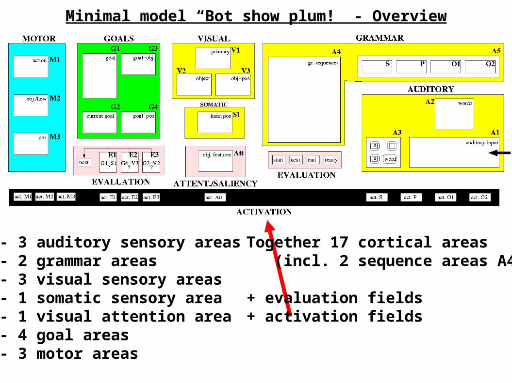
Minimal model “Bot show plum!” - Overview

Minimal model “Bot show plum!” - Overview
- 3 auditory sensory areas

Minimal model “Bot show plum!” - Overview
- 3 auditory sensory areas- 2 grammar areas

Minimal model “Bot show plum!” - Overview
- 3 auditory sensory areas- 2 grammar areas- 3 visual sensory areas

Minimal model “Bot show plum!” - Overview
- 3 auditory sensory areas- 2 grammar areas- 3 visual sensory areas- 1 somatic sensory area

Minimal model “Bot show plum!” - Overview
- 3 auditory sensory areas- 2 grammar areas- 3 visual sensory areas- 1 somatic sensory area- 1 visual attention area

Minimal model “Bot show plum!” - Overview
- 3 auditory sensory areas- 2 grammar areas- 3 visual sensory areas- 1 somatic sensory area- 1 visual attention area- 4 goal areas

Minimal model “Bot show plum!” - Overview
- 3 auditory sensory areas- 2 grammar areas- 3 visual sensory areas- 1 somatic sensory area- 1 visual attention area- 4 goal areas- 3 motor areas

Minimal model “Bot show plum!” - Overview
- 3 auditory sensory areas- 2 grammar areas- 3 visual sensory areas- 1 somatic sensory area- 1 visual attention area- 4 goal areas- 3 motor areas
Together 17 cortical areas (incl. 2 sequence areas A4/G1)

Minimal model “Bot show plum!” - Overview
- 3 auditory sensory areas- 2 grammar areas- 3 visual sensory areas- 1 somatic sensory area- 1 visual attention area- 4 goal areas- 3 motor areas
Together 17 cortical areas (incl. 2 sequence areas A4/G1)
+ evaluation fields
Minimal model “Bot show plum!” - Overview
- 3 auditory sensory areas- 2 grammar areas- 3 visual sensory areas- 1 somatic sensory area- 1 visual attention area- 4 goal areas- 3 motor areas
Together 17 cortical areas (incl. 2 sequence areas A4/G1)
+ evaluation fields+ activation fields

Minimal model “Bot show plum!” - Integration
Input fromrobot sensors -
robot software - simulation environment -

Minimal model “Bot show plum!” - Integration
Input fromrobot sensors -
robot software - simulation environment -
Output to - robot actors - robot software - simulation environment
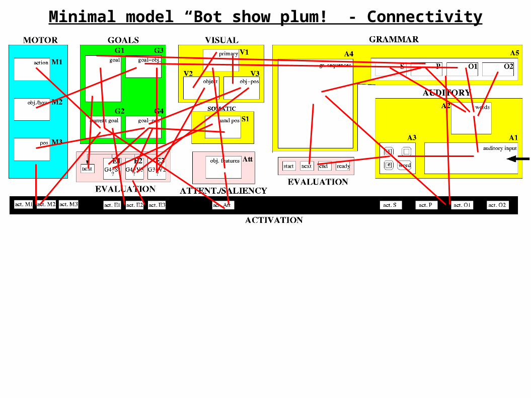
Minimal model “Bot show plum!” - Connectivity

Bot listens to “Bot show plum!”

“Bot show plum!”: Processing of ‘bot’ (1)

“Bot show plum!”: Processing of ‘bot’ (2)

“Bot show plum!”: Processing of ‘bot’ (3)

“Bot show plum!”: Processing of ‘bot’ (4)
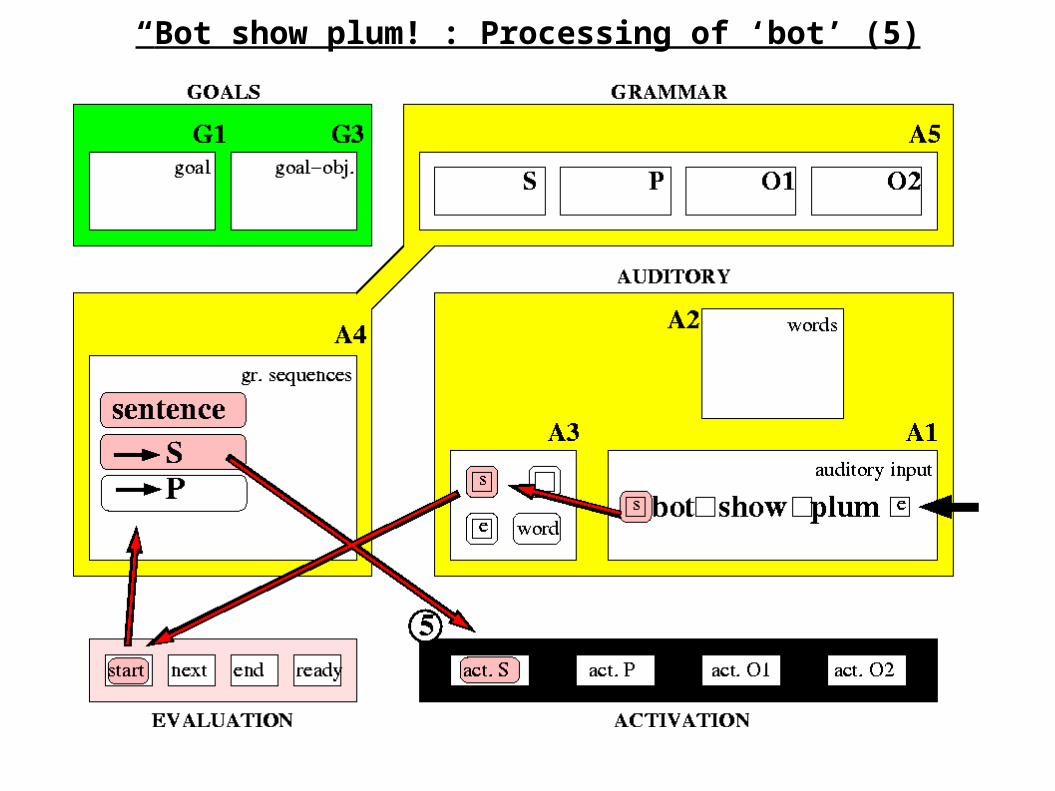
“Bot show plum!”: Processing of ‘bot’ (5)

“Bot show plum!”: Processing of ‘bot’ (6)
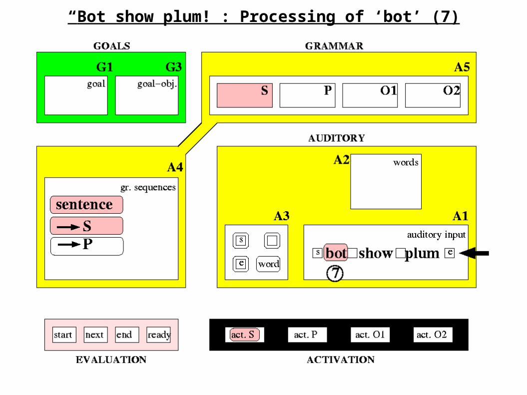
“Bot show plum!”: Processing of ‘bot’ (7)

“Bot show plum!”: Processing of ‘bot’ (8)

“Bot show plum!”: Processing of ‘bot’ (9)

“Bot show plum!”: Processing of ‘bot’ (10)

“Bot show plum!”: Processing of ‘show’ (1)
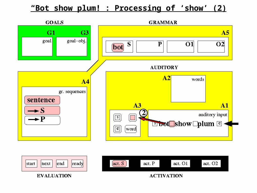
“Bot show plum!”: Processing of ‘show’ (2)
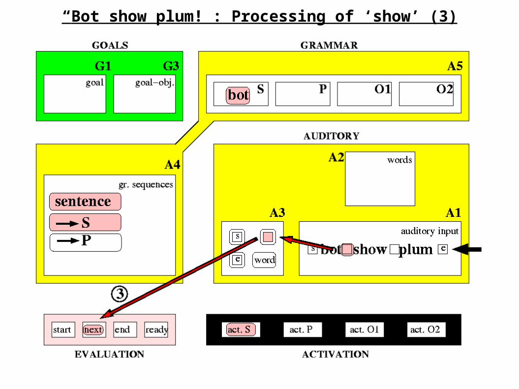
“Bot show plum!”: Processing of ‘show’ (3)
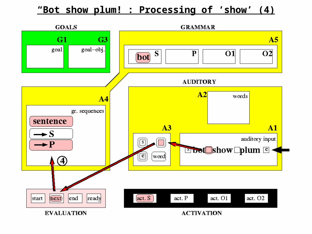
“Bot show plum!”: Processing of ‘show’ (4)

“Bot show plum!”: Processing of ‘show’ (5)

“Bot show plum!”: Processing of ‘show’ (6)

“Bot show plum!”: Processing of ‘show’ (7)

“Bot show plum!”: Processing of ‘show’ (8/9)

“Bot show plum!”: Processing of ‘show’ (10)
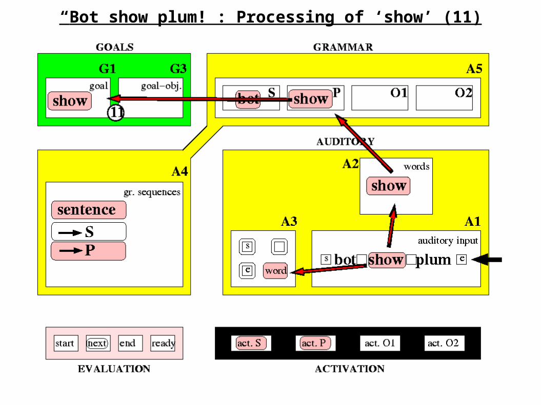
“Bot show plum!”: Processing of ‘show’ (11)

“Bot show plum!”: Processing of ‘show’ (12)

“Bot show plum!”: Processing of ‘plum’ (1)
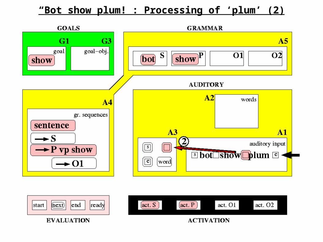
“Bot show plum!”: Processing of ‘plum’ (2)

“Bot show plum!”: Processing of ‘plum’ (3)
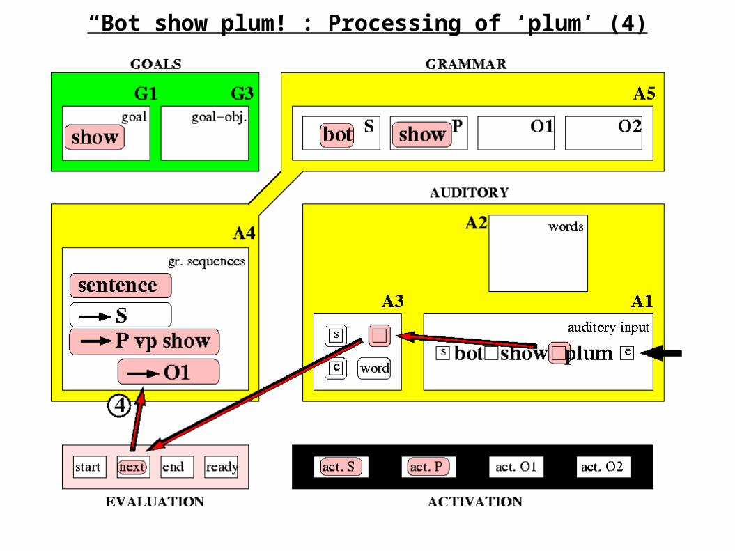
“Bot show plum!”: Processing of ‘plum’ (4)

“Bot show plum!”: Processing of ‘plum’ (5)

“Bot show plum!”: Processing of ‘plum’ (6)

“Bot show plum!”: Processing of ‘plum’ (7)
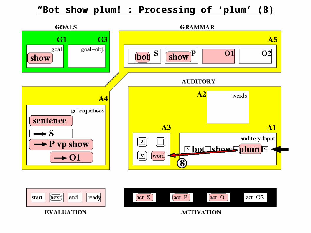
“Bot show plum!”: Processing of ‘plum’ (8)
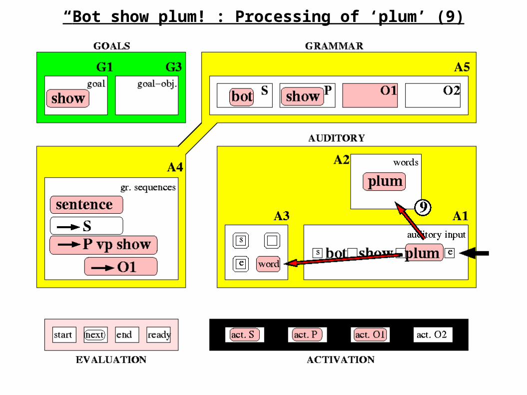
“Bot show plum!”: Processing of ‘plum’ (9)

“Bot show plum!”: Processing of ‘plum’ (10)

“Bot show plum!”: Processing of ‘plum’ (11)

After listening to “Bot show plum!”: Bot knows finally what to do (G1/G3)

Bots reaction to “Bot show plum!”

“Bot show plum!”: Seek plum - Activate motor areas (1)

“Bot show plum!”: Seek plum - Activate motor areas (2)

“Bot show plum!”: Seek plum - Activate motor areas (3)

“Bot show plum!”: Seek plum - Activate motor areas (4)

“Bot show plum!”: Seek plum - Activate motor areas (5)

“Bot show plum!”: Seek plum - Activate motor areas (6)

“Bot show plum!”: Seek plum - Activate motor areas (6/7)

“Bot show plum!”: Seek plum - Activate motor areas (7)
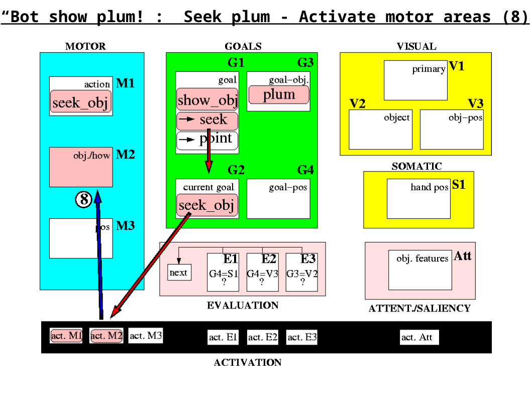
“Bot show plum!”: Seek plum - Activate motor areas (8)

“Bot show plum!”: Seek plum - Activate motor areas (9)

“Bot show plum!”: Seek plum - Motor areas are activated!

“Bot show plum!”: Seek plum - Activate visual attention (1)
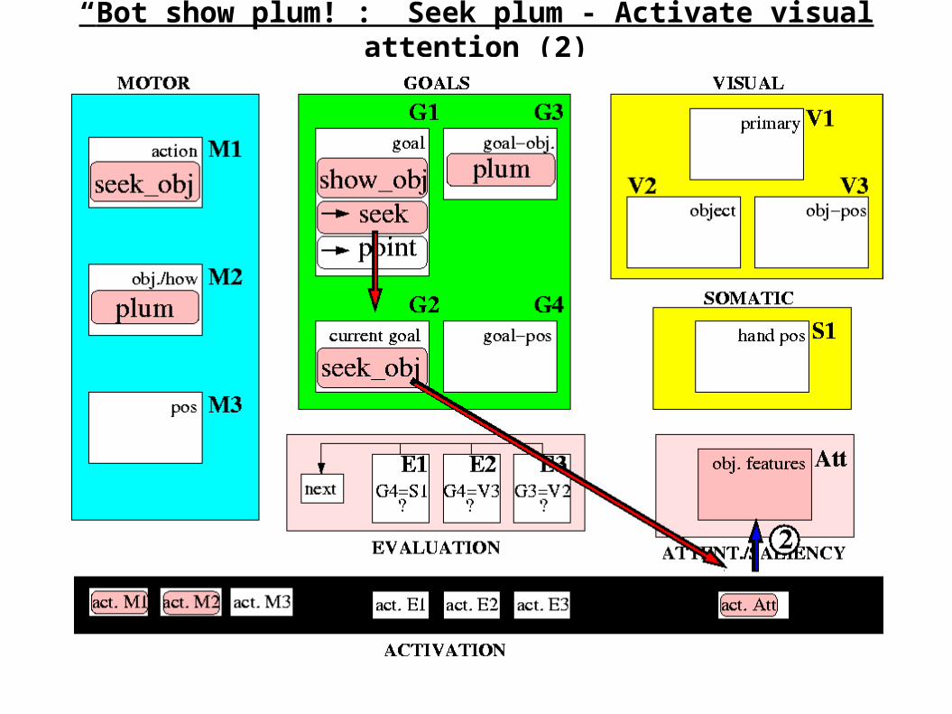
“Bot show plum!”: Seek plum - Activate visual attention (2)

“Bot show plum!”: Seek plum - Activate vis. attention (3)

“Bot show plum!”: Seek plum - Activate vis. attention (4)

“Bot show plum!”: Seek plum - Attention is active!

“Bot show plum!”: Seek plum - Check if plum is visible (1)

“Bot show plum!”: Seek plum - Check if plum is visible (2)

“Bot show plum!”: Seek plum - Check if plum is visible (3)

“Bot show plum!”: Seek plum - Wait until plum is visible!

“Bot show plum!”: Seek plum - plum is visible (1)

“Bot show plum!”: Seek plum - plum is visible (2)

“Bot show plum!”: Seek plum - plum is visible (3)
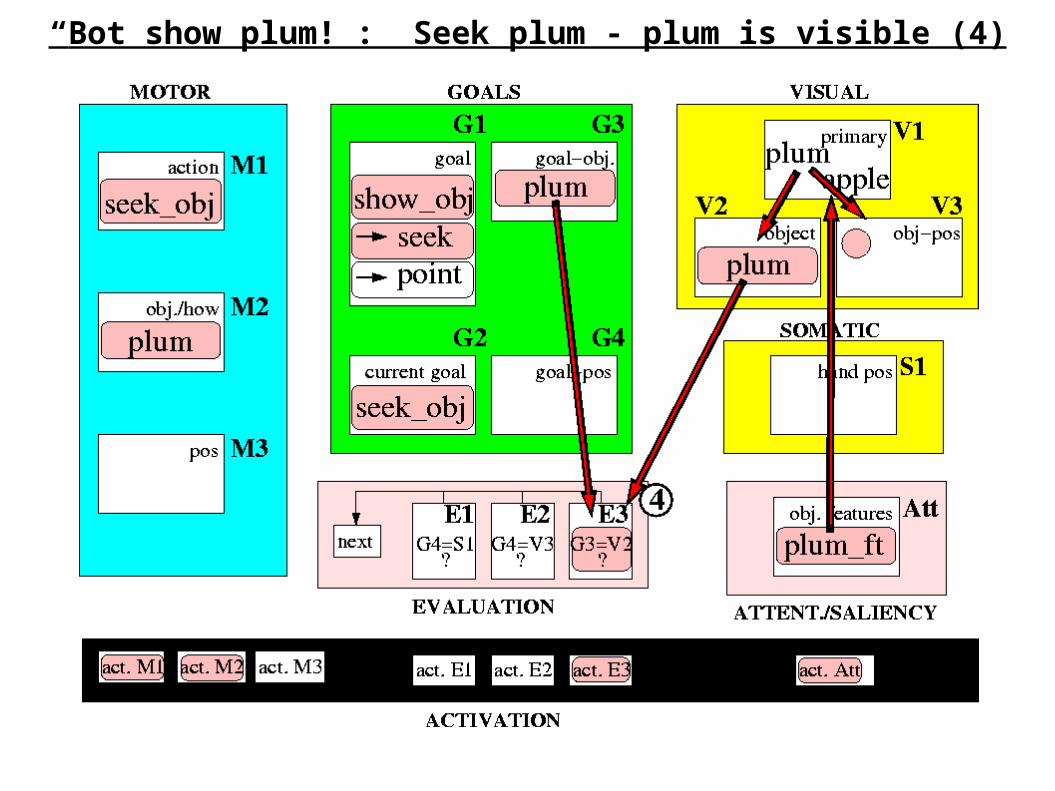
“Bot show plum!”: Seek plum - plum is visible (4)

“Bot show plum!”: Seek plum - plum is visible (5)

“Bot show plum!”: Seek plum - plum is visible (6)

“Bot show plum!”: Plum is found, now point to plum

“Bot show plum!”: point to plum - activate motor areas (1)

“Bot show plum!”: point to plum - activate motor areas (2)

“Bot show plum!”: point to plum - activate motor areas (3)

“Bot show plum!”: point to plum - activate motor areas (4)

“Bot show plum!”: point to plum - activate motor areas (5)

“Bot show plum!”: point to plum - activate motor areas (5/6)

“Bot show plum!”: point to plum - activate motor areas (6)

“Bot show plum!”: point to plum - activate motor areas (7)

“Bot show plum!”: point to plum - activate motor areas (8)

“Bot show plum!”: point to plum - activate motor areas (9)

“Bot show plum!”: point to plum - motor areas are activated!

“Bot show plum!”: point to plum - activate hand position control (1)

“Bot show plum!”: point to plum - activate hand position control (2)

“Bot show plum!”: point to plum - activate hand position control (3)

“Bot show plum!”: point to plum - activate hand position control (4)

“Bot show plum!”: point to plum - activate hand position control (5)

“Bot show plum!”: point to plum - hand position control is active

“Bot show plum!”: point to plum - hand moves to correct position (1)

“Bot show plum!”: point to plum - hand moves to correct position (2)

“Bot show plum!”: point to plum - hand moves to correct position
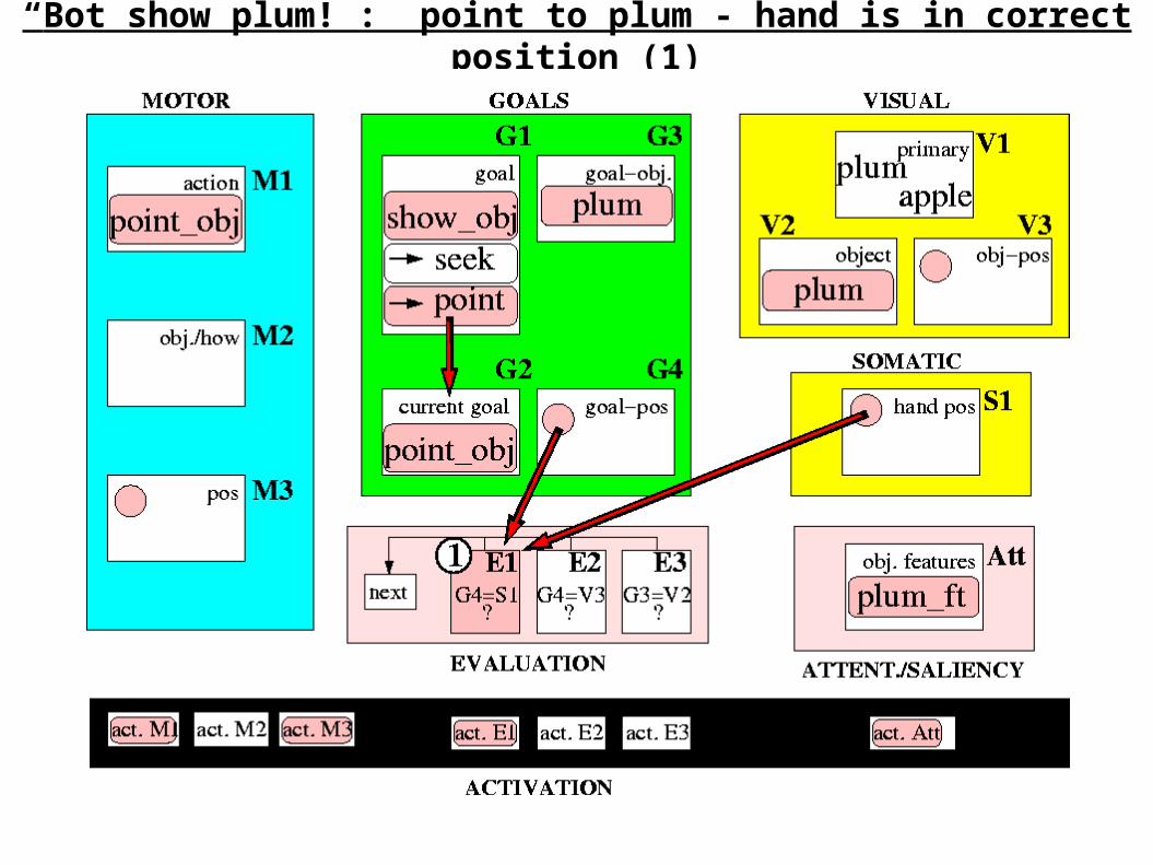
“Bot show plum!”: point to plum - hand is in correct position (1)

“Bot show plum!”: point to plum - hand is in correct position (2)

“Bot show plum!”: Bot has completed the task!

Summary:
- We have proposed a minimal model for „Bot show plum!“ - in principle implementable by using
biological neurons and associative memories
Discussion:
- biologically realistic?
- Modell extensions? - complexer scenarios? - learning? - mirror system?