branch-and-cut-and-price for the robust capacitated
TRANSCRIPT
Branch-and-cut-and-price for the robust
capacitated vehicle routing problem with
knapsack uncertainty
Artur Alves Pessoa, Michael Poss, Ruslan Sadykov, Francois
Vanderbeck
Volume 2018, Number 1
November, 2018

Branch-and-cut-and-price for the robust capacitated vehicle routingproblem with knapsack uncertainty
Artur Alves Pessoaa, Michael Possb,∗, Ruslan Sadykovc, Francois Vanderbeckd
a Universidade Federal Fluminense, Rua Passo da Patria, 156/309-D, Niteroi – RJ, 24210-240, Brazil.b UMR CNRS 5506 LIRMM, Universite de Montpellier, 161 rue Ada Montpellier, France.
c INRIA Bordeaux - Sud-Ouest, 200 avenue de la Vieille Tour, 33405 Talence, France.d IMB, Universite de Bordeaux, 351 cours de la Liberation, 33405 Talence, France.
Abstract
We examine the robust counterpart of the classical Capacitated Vehicle Routing Problem (CVRP).
We consider two types of uncertainty sets for the customer demands: the classical budget polytope
introduced by Bertsimas and Sim (2003), and a partitioned budget polytope proposed by Gounaris
et al. (2013). We show that using the set-partitioning formulation it is possible to reformulate our
problem as a deterministic heterogeneous vehicle routing problem. Thus, many state-of-the-art
techniques for exactly solving deterministic VRPs can be applied for the robust counterpart, and a
modern branch-and-cut-and-price algorithm can be adapted to our setting by keeping the number
of pricing subproblems strictly polynomial. More importantly, we introduce new techniques to
significantly improve the efficiency of the algorithm. We present analytical conditions under which
a pricing subproblem is infeasible. This result is general and can be applied to other combinatorial
optimization problems with knapsack uncertainty. We also introduce robust capacity cuts which
are provably stronger than the ones known in the literature. Finally, a fast iterated local search
algorithm is proposed to obtain heuristic solutions for the problem. Using our branch-and-cut-
and-price algorithm incorporating existing and new techniques, we are able to solve to optimality
all but one open instances from the literature.
Keywords: branch-and-cut-and-price, robust optimization, capacity inequalities, local search
1. Introduction
Vehicle routing problems (VRPs) form a highly studied class of combinatorial optimization
problems with applications in a large number of fields, most often related to freight transporta-
tion and logistics. Vehicle routing concerns distribution of goods between depots and customers.
Distribution is performed by vehicles which use a road network modeled as a graph. A solution
of a VRP is a set of routes each performed by a vehicle starting and ending at its depot such
∗Corresponding authorEmail addresses: [email protected] (Artur Alves Pessoa), [email protected] (Michael Poss),
[email protected] (Ruslan Sadykov), [email protected] (Francois Vanderbeck)
Research papers in Cadernos do LOGIS-UFF are not peer reviewed, authors are responsible for their contents.

Cadernos do LOGIS-UFF L-2018-1 3
that operational constraints are satisfied, requirements of customers are fulfilled, and the trans-
portation cost is minimized. A fundamental variant of VRP is the Capacitated Vehicle Routing
Problem (CVRP), in which a unique product type is delivered from a single depot to customers
using a fleet of identical vehicles. The only operational constraint here is that the total product
demand of clients in a same route should not exceed the vehicle capacity.
The state-of-the-art approaches for exactly solving the CVRP and many other vehicle routing
problems are based on branch-and-cut-and-price algorithms. These approaches formulate the
problem using a set of binary variables, each of which is associated with the selection of a route
that satisfies operational constraints. The number of such variables is usually exponential so that
the linear relaxation of the formulation is solved by column generation. The pricing problem is
a resource constrained elementary shortest path problem, typically solved by a labeling dynamic
programming algorithm (Irnich and Desaulniers 2005). While already quite strong, the continuous
relaxation of these formulations can be further reinforced using cutting planes (Fukasawa et al.
2006) and strong branching can be used to close the gap between the primal and dual bound if
needed. Branch-and-cut-and-price algorithms have witnessed an important progress in the past
12 years: the bidirectional labeling algorithm was introduced by Righini and Salani (2006) to
solve the pricing subproblem faster; an arc elimination by reduced costs (Irnich et al. 2010) was
employed to reduce the size of the graph and to further speed up the labeling algorithm; ng-path
relaxation (Baldacci et al. 2011) replaced the path elementarily requirement in pricing; route
enumeration technique was suggested by Baldacci et al. (2008) in order to close the instance by
a MIP solver when the primal-dual gap is sufficiently low; a limited memory technique for subset
row cuts (Jepsen et al. 2008) and more generally for Chvatal-Gomory rank-1 cuts was proposed
by Pecin et al. (2017b) for limiting the resulting solution time increase in the pricing subproblem.
The branch-and-cut-and-price algorithm of Pecin et al. (2017b), employing the aforementioned
techniques, has proved that it was possible to solve exactly CVRPs much larger than ever before
in reasonable amounts of time. Yet, it neglects to consider that the demands to be picked-up
are rarely known with precision at the time the routes are planned. In the absence of a decision
making tool modeling this uncertainty, decision makers are forced to largely overestimate the
demands or to rely on expensive recourse actions to pick up the additional demands. Fortunately,
different frameworks have arisen in the past decades to take such uncertainty into account when
solving optimization problems, such as stochastic programming (Birge and Louveaux 2011), robust
optimization (Ben-Tal et al. 2009, Ben-Tal and Nemirovski 1998, Kouvelis and Yu 2013), and more
recently, distributionally robust optimization (Wiesemann et al. 2014). Stochastic variants of the
CVRP have been extensively studied in the literature, see Gendreau et al. (1996) for an early
survey and Dinh et al. (2018) for a more recent one and an advanced solution algorithm. Yet,
these approaches result in optimization problems that tend to be significantly more complex than
their deterministic counterparts, making them difficult to apply to large industrial applications.
In addition, these techniques requires exact knowledge about the probability distributions of the

Cadernos do LOGIS-UFF L-2018-1 4
uncertain parameters, which can be hard to obtain in some applications.
Robust and distributionally robust counterparts of the CVRP avoid these two issues by de-
scribing the uncertain demands through either given uncertainty sets or probability distributions
lying in given ambiguity sets. Hence, these approaches assume that only partial information about
the distribution of the uncertain problem data is available. To our knowledge, the first study on
the robust CVRP dates back to Sungur et al. (2008) who consider a variant of the robust CVRP
where travel time is uncertain and the total travel time of each vehicle is bounded. They further
study conditions under which all uncertain parameters reach simultaneously their extreme values,
yielding a deterministic conservative reformulation. Their work was followed by the description
of more general models in Ordonez (2010). Later, Gounaris et al. (2013) study the robust CVRP
and compare several compact mixed-integer formulations for the problems, including formulations
involving recourse variables, modeled with the help of affine decision rules (Ben-Tal et al. 2004).
Gounaris et al. (2013) also study the relationship between the robust CVRP and its chance-
constrained distributionally robust counterpart. The latter problem is addressed more recently
by Ghosal and Wiesemann (2018) where the authors characterize ambiguity sets that make the
problem amenable to efficient numerical solutions. Heuristic algorithms have also been developed
for the robust CVRP, among which Gounaris et al. (2016) who develop an adaptive memory
programming framework for the problem.
This previous research studies have provided excellent exact or heuristic solutions to robust
and distributionally robust CVRP, allowing one to solve larger instances than before. Yet, perfor-
mance still stand significantly behind those offered by the recent algorithms for the deterministic
CVRP (Pecin et al. 2017b). One theoretical reason explaining this difference lies in the complex-
ity of robust optimization with arbitrary uncertainty sets. For instance, it is known that even
optimizing a linear function over a robust robust knapsack constraint (an important substructure
of the CVRP) is NP-hard in the strong sense for arbitrary uncertainty sets (Talla Nobibon and
Leus 2014), contrasting with the weak NP-hardness of the deterministic case. In fact, it is well-
known that arbitrary uncertainty sets make robust combinatorial optimization problems much
harder than their deterministic counterparts, and most polynomially solvable problems become
NP-hard when considering robust variants with arbitrary uncertainty sets (Aissi et al. 2009).
This complexity gap has motivated the introduction of structured uncertainty sets that lead to
robust counterparts almost as easy as the deterministic problems, namely, budgeted uncertainty
sets (Bertsimas and Sim 2003). The latter models the uncertainty on demands through nominal
values, deviations, and a budget of uncertainty. Then, any demand vector in the budgeted uncer-
tainty polytope has a number of components that deviate from their mean that is controlled by
the budget of uncertainty. Bertsimas and Sim (2003) prove that budgeted uncertainty leads to
robust counterparts of min-max problem with cost uncertainty that are fundamentally as easy as
the deterministic problems. Essentially, Bertsimas and Sim (2003) have shown that the optimal
solution of a min-max combinatorial optimization problem with feasibility set X ⊆ {0, 1}n with

Cadernos do LOGIS-UFF L-2018-1 5
cost uncertainty can be obtained by solving n deterministic problems with perturbed cost vec-
tors. Their results have been improved in subsequent works by Alvarez-Miranda et al. (2013), Lee
and Kwon (2014), Lee et al. (2012) and extended to knapsack uncertainty sets by Poss (2018).
While Bertsimas and Sim (2003) focused on cost uncertainty, Alvarez-Miranda et al. (2013) and
Goetzmann et al. (2011) have independently shown how to extend these results to optimiza-
tion problems with uncertain constraint parameters. In addition to its desirable computational
properties, budgeted uncertainty sets also benefit from probabilistic guarantees, providing safe
approximations to chance constraints (Bertsimas and Sim 2004, Poss 2013, 2014). Unfortunately,
applying the above results to classical formulations of the CVRP with m vehicles would lead to
solving O(nm) deterministic CVRP with perturbed data, explaining the current lack of interest
in solving the robust CVRP with these techniques.
The main achievement of our present work is to bridge the gap between the advanced solution
algorithms available for the deterministic CVRP and the iterative algorithms initiated by Bertsi-
mas and Sim (2003). Specifically, we show that, by using the set-partitioning formulation, one can
transpose all classical techniques of the CVRP to its robust counterpart. With that approach,
we solve for the first time many instances proposed in the literature for the robust CVRP. In
the process, we also introduce new techniques that apply to more general robust combinatorial
optimization problems under knapsack uncertainty. We can summarize the contributions of our
paper as follows.
1. We show how to reformulate the robust CVRP with knapsack uncertainty as a deterministic
heterogeneous VRP that involves a polynomial number of pricing subproblems which are
not harder than the pricing problem for the deterministic CVRP.
2. Using complementary slackness conditions, we can empirically verify that many pricing
subproblems are infeasible, thus reducing their number. This technique can be applied to
any robust combinatorial optimization problem with knapsack uncertainty.
3. We introduce new robust capacity inequalities and prove that they are stronger than those
proposed by Gounaris et al. (2013).
4. We develop a fast iterated local search heuristic for the problem which uses four neighbor-
hoods. We show how to check the feasibility of a neighbor either exactly or approximately
in constant time. The heuristic is shown to empirically outperform the one by Gounaris
et al. (2016).
5. Combining these new developments with a deterministic state-of-the-art branch-and-cut-
and price algorithm for the heterogeneous VRP, we are able to solve to proven optimality
all but one instance for the partition uncertainty set considered previously by Gounaris et al.
(2013).
6. We generate new robust CVRP instances for the classic cardinality constrained uncertainty
set and show experimentally that they are more difficult than the ones proposed by Gounaris
et al. (2013). The smallest open instance has only 50 customers.

Cadernos do LOGIS-UFF L-2018-1 6
The rest of the paper is structured as follows. Section 2 defines the uncertainty sets, states the
extension of the the result from Bertsimas and Sim (2003) to knapsack uncertainty and provides
extensions to reduce the number of problems solved. Section 3 describes the set-partitioning
formulation that can be combined with the results from Section 2, and presents the key features
of our branch-and-cut-and-price algorithm. Sections 4 and 5 detail our capacity inequalities
and primal heuristics, respectively. The numerical experiments are presented in Section 6 and
concluding remarks are provided in Section 7. Proofs, detailed numerical experiments, further
examples and algorithmic specifications are deferred to the appendix. The latter also provides
raw results to ease reproducibility of our experiments.
2. Robust model
Let G = (V,A) be a complete digraph with nodes V = {0, 1, . . . , n} and arcs {(i, j) ∈ V × V :
i 6= j}. Node 0 ∈ V represents the unique depot, and each node i ∈ V 0 = V \ {0} corresponds
to a customer with demand di ∈ IR+. The depot hosts m homogeneous vehicles of capacity C.
Each vehicle incurs a transportation cost cij ∈ IR+ if it traverses the arc (i, j) ∈ A. The objective
is to find a set of m routes starting and ending at the depot, each one serving a total demand of
at most C, such that each customer is visited exactly once and the total transportation cost is
minimized.
2.1. Uncertainty polytopes
The demand vector d can take any value in a given polytope D that is included in the box
[d, d + d] defined by the vectors d, d ∈ IRn+, where d represent the nominal values and d the
deviations. Notice that it is irrelevant to consider downward deviations of d in our context
because we focus on capacity constraints for which downward deviations of d will not lead to
infeasibility of the constraints. We consider in this work two different polytopes. The first one
is the budgeted polytope introduced in Bertsimas and Sim (2003, 2004), and widely used in the
robust combinatorial optimization literature since then. Given Γ ∈ IR+, the budgeted polytope
is given by
Dcard =
d ∈ IRn+
∣∣∣∣∣∣ di = di + ηidi, i ∈ V 0,∑i∈V 0
ηi ≤ Γ, 0 ≤ η ≤ 1
.
The second polytope we are interested in comes from Gounaris et al. (2013) where the authors
consider a partition VC = {V1, . . . , Vs} of V 0 and non-negative numbers b1, . . . , bs ∈ IR+.
Dpart =
d ∈ IRn+
∣∣∣∣∣∣ di = di + ξi, i ∈ V 0,∑i∈Vk
ξi ≤ bk, k = 1, . . . , s, 0 ≤ ξ ≤ d
.

Cadernos do LOGIS-UFF L-2018-1 7
To compare the two polytopes, one might use the relation ξi = diηi which underlines the fact
that Dcard constrains the number of elements of d that deviate simultaneously from their nominal
values, while Dpart constrains the total amount of deviation for each partition of the uncertainty
sources set. Restraining the total amount of deviation as in Dpart has been used in other contexts,
such as robust scheduling in Tadayon and Smith (2015).
Let us consider a given combinatorial optimization problem P. Further, let Y ⊆ {0, 1}n be a
set of binary vectors such that the feasibility set of P contains exactly the vectors in Y that also
satisfies the following robust constraint
n∑i=1
(di + ηidi)yi ≤ C, ∀η ∈ H, (1)
where H =
{η ∈ [0, 1]n
∣∣∣∣∣ ∑i∈Vk wiηi ≤ bk, k = 1, . . . , s
}, where wi ≥ 0 for i = 1, . . . , n. In the
context of the CVRP, P decides which customers are visited by a given vehicle and each vector
in Y represent a set of customers that could be visited by the vehicle.
Note that Dknap = {d | di = di+ηidi, ∀i ∈ {1, . . . , n}, η ∈ H} generalizes both Dpart and Dcard.For the former, we set wi = di, and for the latter, s = 1, b1 = Γ, and w1 = · · · = wn = 1. Note
also that, assuming w.l.o.g. that wi > 0 for i = 1, . . . , n, (1) is equivalent to
d>y + max
ξ∈Ξ
{n∑i=1
diwiξiyi
}≤ C, (2)
where Ξ =
{ξ ∈ IRn
+
∣∣∣∣∣ ξ ≤ w, ∑i∈Vk ξi ≤ bk, k = 1, . . . , s
}.
2.2. Reducing robust problems to deterministic ones
In the following, we give an alternative definition for (2) that helps to explore the ability
to solve the deterministic counterpart of P as a subproblem, and also allows us to reduce the
solution space of the subproblems to be solved. For that, it is useful to rewrite (2) replacing the
linear programming problem on its left-hand side by its dual:
d>y + min
θ,z≥0
{b>θ + w>z s.t. zi + θk(i) ≥
diwiyi, i = 1, . . . , n
}≤ C, (3)
where k(i) is the only value of k such that i ∈ Vk. By observing the one-to-one correspondence
between the z variables and the constraints in (3), each zi, for i = 1, . . . , n, can be replaced by
max{0, diwi yi − θk(i)}. This leads to the equivalent constraint
d>y+ min
θ∈IRs+
{b>θ +
n∑i=1
max{0, diyi − wiθk(i)}
}= d
>y+ min
θ∈IRs+
{b>θ +
n∑i=1
max{0, di − wiθk(i)} yi
}

Cadernos do LOGIS-UFF L-2018-1 8
= minθ∈IRs+
{b>θ +
n∑i=1
(di + max{0, di − wiθk(i)}) yi
}≤ C. (4)
Now, let dθi = di + max{0, di − wiθk(i)}, Y knap = {y ∈ Y | d>y ≤ C,∀d ∈ Dknap}, and
Y knapθ = {y ∈ Y | b>θ + (dθ)>y ≤ C}, for each θ ∈ IRs
+. Finally, let θ0k = 0 for k = 1, . . . , s,
θik(i) = di/wi for i = 1, . . . , n, and
Θ = ({0} ∪ {θik(i) | i ∈ V1})× · · · × ({0} ∪ {θik(i) | i ∈ Vs}). (5)
The following theorem, the proof of which is is deferred to Section Appendix A.1 of the appendix,
requires that both di and wi are strictly greater than zero for i = 1, . . . , n. However, since they
may be set as small as needed, this assumption is not restrictive from the practical point of view.
Theorem 1. Y knap =⋃θ∈Θ
Y knapθ
Theorem 1 shows that P under the robust constraint (1) can be solved by taking the best
solution among all instances of its deterministic counterpart generated using Y knapθ , for all θ ∈ Θ.
The uncertainty sets covered by the theorem are more restricted than those studied in Theorem 3
from Poss (2018). This being said, the formula for Θ is simpler than the one from Poss (2018),
which involves solving linear systems of equations. Notice also that the result has been known for
a while in the case of Dcard (Alvarez-Miranda et al. 2013, Bertsimas and Sim 2003, Goetzmann
et al. 2011, Lee and Kwon 2014), in which case Θ′ = {0, d1, d2, . . . , dn}. For the later set, Lee and
Kwon (2014) further showed that only a subset of Θ′ needs to be considered.
Theorem 2 (Lee and Kwon (2014)). Consider Dcard and suppose w.l.o.g. that d1 ≥ d2 ≥ · · · ≥dn ≥ dn+1 = 0. Define Θcard = {dΓ+1, dΓ+3, dΓ+5, . . . , dΓ+γ , 0} where γ is the largest odd integer
such that Γ + γ < n+ 1. It holds that for any y ∈ {0, 1}n
argminθ∈IR1
+
(Γθ + (d+ max{0, d− θ})>y
)∩Θcard 6= ∅.
Defining Y card = {y ∈ Y | d>y ≤ C,∀d ∈ Dcard}, and Y cardθ = {y ∈ Y |Γθ + (d + max{0, d −
θ})>y ≤ C}, for each θ ∈ IRs+, Theorem 2 implies that the robust feasibility set Y card can be
reformulated as the union of the deterministic feasibility sets corresponding to the elements of
Θcard ⊂ Θ.
Corollary 1. Y card =⋃
θ∈ΘcardY cardθ
Let us turn to the implication of Theorem 1 to set Dpart. We see that applying formula (5)
to Dpart leads to a set having a cardinality that no longer depends on n. Let Θpart = {0, 1}s.
Lemma 1. If wi = di for each i = 1, . . . , n, then Θ = Θpart.

Cadernos do LOGIS-UFF L-2018-1 9
2.3. Reducing the cardinality of Θ
We explain next how to reduce even further the number of elements of Θ that need to be
considered. Our approach works in two steps. First, we define
Y knapθ =
y ∈ Y knapθ
∣∣∣∣∣∣∑i∈Vk
wiyi ≤ bk,∀k ∈ {1, . . . , s} | θk = 0,
∑i∈Vk
di>wiθk
wiyi ≤ bk ≤∑i∈Vk
di≥wiθk
wiyi, ∀k ∈ {1, . . . , s} | θk > 0
.
We will show that one needs only to consider an element θ ∈ Θ if Y knapθ is non-empty, by showing⋃
θ∈Θ
Y knapθ =
⋃θ∈Θ
Y knapθ . (6)
In fact, proving (6) would not be enough to cover Corollary 1 because the latter involves a proper
subset Θcard ⊂ Θ. Hence, the theorem below, the proof which is provided in Section Appendix
A.2 of the appendix, generalizes slightly (6), by considering any set Θ∗ ⊆ Θ large enough to
contain all minimizers of the left-hand side of (4).
Theorem 3. Let Θ∗ ⊆ Θ be such that for each y ∈ Y
argminθ∈IRs+
(b>θ + (dθ)>y
)∩Θ∗ 6= ∅. (7)
Then, it holds that⋃
θ∈Θ∗Y knapθ =
⋃θ∈Θ∗
Y knapθ
The constraints that are added in Y knapθ may destroy the structure of the original deterministic
problem, making the corresponding optimization problem harder to solve. Here comes the second
step of our approach: we use these constraints only to find out whether a given set Y knapθ is empty,
in which case the corresponding θ can be removed from Θ∗. This is formalized in the next result.
Corollary 2. Let Θ∗ ⊆ Θ that satisfies (7) and consider a set Θ such that {θ ∈ Θ∗ | Y knapθ 6=
∅} ⊆ Θ. It holds that Y knap =⋃θ∈Θ
Y knapθ .
For an arbitrary set Y , testing the emptiness of Y knapθ can be NP-hard in the strong sense, so
that we test instead the feasibility of a larger and simpler set. The later is defined by relaxing the
combinatorial structure Y to {0, 1}n and removing the first two groups of constraints of Y knapθ .

Cadernos do LOGIS-UFF L-2018-1 10
Formally, we define K(θ) = {k ∈ {1, . . . , s} | θk > 0}, Vk = {i ∈ Vk | di ≥ wiθk}, and
Bknapθ =
y ∈ {0, 1}n | b>θ + (dθ)>y ≤ C,∑i∈Vk
wiyi ≥ bk,∀k ∈ K(θ)
.
Clearly, Y knapθ ⊆ Bknapθ . What is more, testing the emptiness of Bknapθ can be done by solving
z∗ = miny∈{0,1}n
(dθ)>y
∣∣∣∣∣∣∑i∈Vk
wiyi ≥ bk,∀k ∈ K(θ)
=∑
k∈K(θ)
miny∈{0,1}|Vk|
∑i∈Vk
dθi yi
∣∣∣∣∣∣∑i∈Vk
wiyi ≥ bk
=
∑k∈K(θ)
miny∈{0,1}|Vk|
∑i∈Vk
dθi yi
∣∣∣∣∣∣∑i∈Vk
wiyi ≥ bk
.
Hence, z∗ can be computed in pseudo-polynomial time by solving a knapsack problem for each
k ∈ K(θ). If one of these knapsack problem is infeasible, then we set z∗k = ∞. Then, having
z∗ > C−b>θ implies that Bknapθ is empty. For the special cases of Dcard and Dpart this computation
is much simpler and can be done in a polynomial time as we show next.
Clearly, Θcard satisfies (7) whenever s = 1, b1 = Γ, and w1 = · · · = wn = 1, so that the
Corollary 2 can be applied to reduce even further the number of elements considered both in
Corollary 1 and Lemma 1. In this case, one can conclude that Bknapθ is empty (for θ > 0)
whenever
miny∈{0,1}n
∑i∈{1,...,n} | di≥θ
dθi yi
∣∣∣∣∣∣∑
i∈{1,...,n} | di≥θ
yi = Γ
> C − Γθ.
Note that the minimum is attained at the left-hand side of the previous inequality when yi = 1
for the indices i that correspond to the Γ smallest values of di that are not smaller than θ.
In the case of Dpart, we see that θik(i) = 1, so that Vk = Vk and dθi = di. Now, we further
assume that d = κd for some scalar κ > 0 (which is true for all current literature instances), and
consider the linear relaxation of the counterpart of Bknapθ for Dpart
Ipartθ =
y ∈ [0, 1]n | b>θ + d>y ≤ C,
∑i∈Vk
κdiyi ≥ bk,∀k ∈ K(θ)
.
Clearly, Y partθ ⊆ Ipartθ . Further, miny∈[0,1]|Vk|
{∑i∈Vk diyi
∣∣∣∑i∈Vk κdiyi ≥ bk}
= bk/κ for each
k ∈ K(θ), so that the counterpart of z∗ for Dpart is (b>θ)/κ. Hence, Ipartθ is necessarily empty
when (b>θ)/κ > C − b>θ.For both Dcard and Dpart, the set Θ can be computed in a pre-processing phase.
Cadernos do LOGIS-UFF L-2018-1 11
3. Set partitioning formulation and the solution algorithm
3.1. Deterministic problem
We describe in this section the set partitioning formulation used in our branch-and-cut-and-
price algorithm. Let us start with the deterministic version of the problem and define R0 as the
set of all unconstrained elementary routes in G starting and ending at the depot. For each r ∈ R0,
we denote the cost of the route by cr, and indicate whether node i (resp. arc (i, j)) pertains to
the route by the binary number ari (resp. δrij). Then, we describe the set of feasible routes for the
CVRP with demand vector d ∈ IRn+ as
R =
r ∈ R0
∣∣∣∣∣∣∑i∈V0
aridi ≤ C
.
The classical path formulation for the CVRP relies on a set of binary variables, denoted by λ,
where λr is equal to 1 iff route r is part of the optimal solution. We obtain the following integer
linear programming formulation
min∑r∈R
crλr, (8)
s.t.∑r∈R
ariλr = 1, i ∈ V0, (9)∑r∈R
λr = m, (10)
λr ∈ Z, r ∈ R, (11)
In the above formulation, constraints (9) ensure that each customer is covered by exactly one
vehicle, while constraint (10) sets the number of used vehicles to m.
The above integer program typically contains too many variables, so when solving this program
by branch-and-bound, one generally solve the linear programming relaxation using a column
generation procedure, i.e., generating the routes dynamically. Let R ⊆ R be the set of routes
generated so far, the restricted master linear program is obtained from (8)–(11) by replacing R
with R. Given an optimal dual solution (π∗, σ∗) to the linear programming relaxation of (8)–(11)
with R, where π∗ ∈ IRn and σ∗ ∈ IR, we generate new routes by solving the pricing problem
minr∈R
c∗r , (12)
where c∗r = cr −∑
i∈V0ariπ∗i −mσ∗.

Cadernos do LOGIS-UFF L-2018-1 12
3.2. Robust counterpart
When the demand of the clients can take any value in Dknap, the set of feasible routes is
reformulated as
Rknap =
r ∈ R0
∣∣∣∣∣∣∑i∈V0
aridi ≤ C, ∀d ∈ Dknap .
Applying Corollary 2 to Rknap, we obtain
Rknap =⋃θ∈Θ
Rθ, (13)
where
Rθ =
r ∈ R0
∣∣∣∣∣∣∑i∈V0
aridθi ≤ C − b>θ
.
Equation (13) underlines that the set of routes that are feasible for the robust capacity constraint is
nothing else than the union of sets of routes feasible for different deterministic capacity constraints.
Replacing R by Rknap in (8)–(11), and using (13), we obtain the path formulation for the robust
CVRP
min∑θ∈Θ
∑r∈Rθ
crλr, (14)
s.t.∑θ∈Θ
∑r∈Rθ
ariλr = 1, i ∈ V0, (15)
∑θ∈Θ
∑r∈Rθ
λr = m, (16)
λr ∈ Z, θ ∈ Θ, r ∈ Rθ. (17)
Similarly, the robust counterpart of the pricing problem (12) is
minr∈Rknap
c∗r = minr∈
⋃θ∈Θ Rθ
c∗r = minθ∈Θ
minr∈Rθ
c∗r ,
which can be decomposed into subproblems, one for each θ ∈ Θ.
3.3. branch-and-cut-and-price algorithm
To solve formulation (14)–(17), we adopt the branch-and-cut-and-price method by Sadykov
et al. (2017) which is the state-of-the-art algorithm for the (heterogeneous) vehicle routing problem
with time windows. The extension to our problem is the following: set of vehicle types here
corresponds to set Θ; vehicle type θ ∈ Θ is characterized by specific vector dθ of customer
demands and vehicle capacity C − b>θ; the limit m on the number of vehicles is global over all
vehicle types; and there are no time windows. In the reminder of this subsection, we briefly

Cadernos do LOGIS-UFF L-2018-1 13
mention the techniques used in the algorithm. The reader is invited to read the original paper to
obtain the detailed description.
In the algorithm, the linear relaxation of the formulation (14)–(17) is solved by column gener-
ation, stabilized using the automatic dual price smoothing technique by Pessoa et al. (2018). Each
pricing subproblem θ ∈ Θ is solved over the ng-path relaxation (Baldacci et al. 2011) of Rθ by
the bi-directional bucket graph based labelling algorithm proposed by Sadykov et al. (2017). The
main advantage of this labelling algorithm over another recent one by Pecin et al. (2017b) in our
setting is that the former can take into account real-valued customer demands without negative
impact on its performance. The ng-path relaxation is dynamically adjusted using the approach
of Bulhoes et al. (2018). The bucket arcs in the bucket graphs are fixed using reduced cost ar-
guments to simplify the pricing subproblems, as shown in Sadykov et al. (2017). We separate
capacity cuts which are specific for the robust CVRP and which are presented below in Section 4.
We also separate generic rank-1 Chvatal-Gomory cuts for up to 5 rows (Pecin et al. 2017a). Lim-
ited memory technique by Pecin et al. (2017b) is used to decrease the negative impact of rank-1
cuts on the difficulty of the pricing subproblems. Strong branching on edge variables is performed
as in Pecin et al. (2017b). Elementary route enumeration procedure proposed by Baldacci et al.
(2008) is employed to enumerate routes with reduced costs smaller that the current primal-dual
gap. If the number of enumerated routes is small enough, the current branch-and-bound node is
solved by the Cplex MIP solver. The initial feasible solution is obtained by the specific iterated
local search heuristic which we describe in Section 5.
4. Capacity inequalities
Let xij be a binary variable equal to 1 iff there is a vehicle going though arc (i, j). Then, for
any subset of customers S ⊆ V , the rounded capacity inequalities, introduced by Laporte and
Nobert (1983), state that the number of vehicles entering S must not be smaller than the total
demand of the customers in S divided by the vehicle capacity. Stated formally for the robust
problem, we obtain ∑i∈V \S
∑j∈S
xij ≥
⌈1
Cmaxd∈D
∑i∈S
di
⌉, S ⊆ V 0, (18)
which has already been used by Gounaris et al. (2013) for the robust CVRP in the two-index
vehicle flow formulation, here referred to as RVRP-2IF. The maximization overD can be computed
in polynomial time for both uncertainty polytopes considered. For Dcard, one must rely on a
sorting algorithm that ranks the elements of S ∩ Vk according to the non-decreasing values of di.
For Dpart, the maximum can be directly computed as
maxd∈Dpart
∑i∈S
di =∑i∈S
di +
s∑k=1
min
bk, ∑i∈S∩Vk
di
.

Cadernos do LOGIS-UFF L-2018-1 14
Notice finally that (18) can be written in terms of variables λ using the relation xij =∑θ∈Θ
∑r∈Rθ δ
rijλr. We present next a reinforcement of the capacity inequalities.
Let r(S) denote the right-hand side of (18), which is a lower bound on the number of vehicles
required to serve all demand of vertices in S. We remark that the lower bound can be weak if
many routes are used. To understand why, consider the following partition S = S1 ∪ · · · ∪ St and
suppose that each route serves the nodes from one set of the partition. It holds that
t∑`=1
maxd∈D
∑i∈S`
di ≥ maxd∈D
∑i∈S
di,
and the inequality is likely to hold strictly. What is more, the difference between the two sides of
the inequality tends to increase with the number of elements in the partition, therefore reducing
the quality of the bound r(S) when the number of routes used is large.
In order to strengthen (18), we define next a new lower bound r(S) on the number of routes
required to visit S, which tends to be larger than r(S) when t is large. Let us formulate the
number of vehicles required to cover the customers of S as an integer program based on the
reformulation (14)–(17). Specifically, we introduce the integer variable wθ which represents how
many vehicles of type θ are used, each of which having a capacity C−b>θ, and the binary variable
viθ which is equal to 1 iff customer i is affected to a vehicle of type θ (variables v can be related
to variables λ used in (14)–(17) through viθ =∑
r∈Rθ ariλr). We obtain
min∑θ∈Θ
wθ, (19)
s.t.∑θ∈Θ
viθ ≥ 1, i ∈ S, (µi) (20)
∑i∈S
dθi viθ ≤ (C − b>θ)wθ, θ ∈ Θ, (νθ) (21)
wθ ∈ Z, θ ∈ Θ, viθ ∈ Z, i ∈ V, θ ∈ Θ. (22)
where the corresponding dual variables of the continuous relaxation are denoted between paren-
thesis. In this formulation, (19) represents the minimum number of routes required to serve S,
(20) ensures that every customer in S is served, and (21) avoids using more than the available
capacity for each θ ∈ Θ. Solving (19)–(22) for each set S would provide the tightest value for
the right-hand-side of (18). Solving all these integer programs is impractical so that we consider
instead the values of the their continuous relaxation, which we denote r(S). Taking the dual of
the continuous relaxation of (19)–(22), we obtain
r(S) = max∑i∈S
µi,
s.t. µi ≤ dθi νθ, i ∈ S, θ ∈ Θ,

Cadernos do LOGIS-UFF L-2018-1 15
(C − b>θ) νθ ≤ 1, θ ∈ Θ,
µ, ν ≥ 0.
As a result, we have that
r(S) =∑i∈S
minθ∈Θ
dθiC − b>θ
. (23)
We give in Section Appendix B of the appendix three examples that show that (24) improves
upon (18) but there are cases where dr(S)e is smaller than r(S). These examples show that the
strongest capacity inequalities are given by∑i∈V \S
∑j∈S
xij ≥ max{dr(S)e, r(S)} S ⊆ V 0. (24)
This being said, the advantage of using dr(S)e instead of the right-hand side of (24) is that the
former allows to use the separation procedures proposed in Lysgaard et al. (2004), with modified
demands. For that, each demand di is replaced by minθ∈Θ{dθi /(C−b>θ)}, and the vehicle capacity
is set to 1. Since the available implementation of this separation procedure requires that all
demands and the vehicle capacity are integer, we multiply them by a large scale factor and round
them properly to ensure the validity of the cuts. In practice, we have both types of separation
procedures: one specialized in the separation of (24), and another one that uses the procedure of
Lysgaard et al. (2004) and replaces the violated cuts by the equivalent ones of (24).
We conclude the section by showing how to further strengthen the proposed robust capacity
cuts for the specific case of Dpart, with the additional assumption that the demand deviations
are proportional to their nominal values. Namely, we assume that di = κdi for all i ∈ V 0 for
some κ > 0. The following theorem presents an even stronger version of the capacity inequalities;
its proof and the proof of the subsequent proposition are provided in Sections Appendix A.3
and Appendix A.4 of the appendix.
Theorem 4. The inequality∑
i∈V \S
∑j∈S
xij ≥ r(S) is valid for the robust CVRP with Dpart, where
r(S) =s∑
k=1
⌊qk(S)γk
⌋+
⌈s∑
k=1
qk(S)+min{bk,κqk(S)}C
⌉, γk = max
{C
1+κ , C − bk}
, qk(S) =∑
i∈S∩Vkdi and
qk(S) = qk(S)− γk⌊qk(S)γk
⌋for k = 1, . . . , s.
Proposition 1. r(S) ≥ max{dr(S)e, r(S)} always holds and can be strict in some cases.
We separate the robust capacity inequalities at each node of the branch-and-bound tree using a
straightforward extension of the separation heuristic used in Uchoa et al. (2008). For completeness,
its description in is provided Section Appendix C.1 of the appendix.

Cadernos do LOGIS-UFF L-2018-1 16
5. Heuristics
Efficient primal heuristics are usually required to provide good quality upper bounds on the
optimal cost before running exact algorithms. For Dpart, Gounaris et al. (2016) proposed the
AMP heuristic and showed that it helps the previously proposed branch-and-cut (BC) algorithm
(Gounaris et al. 2013) to solve additional instances. Here, we develop an iterated local search
(ILS) heuristic with variable neighborhood search (VNS) in the same spirit as Penna et al. (2013),
which handles both Dpart and Dcard. This heuristic procedure is improved by a data structure
specially designed to allow a faster evaluation of neighborhood solutions. In the next subsection,
we show some properties of robust solutions explored by this data structure. Then, we give the
full algorithm description in the subsection that follows.
5.1. Vehicle routing neighborhoods
A large number of neighborhoods known for vehicle routing problems (Vidal et al. 2013) can
be extended to the robust CVRP. In this paper, we consider four neighborhoods: two intra-route
and two inter-route. The intra-route neighborhoods are subpath inversions (2-OPT) and single
customer moves between positions of the same route (reinsertion), and the inter-route ones are
single-point crossovers of two routes (2-OPT∗) and single customer moves from one route to
another (insert). For all these neighborhoods, the cost of a neighbor solution can be evaluated in
O(1) time by updating the cost of the original solution considering only the costs of edges that
change. For the deterministic version of the problem, a similar approach can be applied to check
the feasibility of each neighbor in O(1) time at the cost of maintaining, for each customer, the
total demand served by the corresponding route up to that point, which is updated in linear time
upon every change in the incumbent solution. The techniques present here allow one to check the
feasibility of neighbor solutions exactly in O(s) time for Dpart, and approximately in O(1) time for
Dcard, also at the cost of updating data structures whenever the incumbent solution is replaced.
In the latter case, the time required by such updates is linear on the route length, but experiments
below show that the proposed technique substantially reduces the overall algorithm run time by
avoiding many exact tests. Moreover, as pointed out in Vidal et al. (2014), any local-search move
composed of a bounded number of edge exchanges and node relocations can also be viewed as
a recombination of a bounded number of subroutes from an incumbent solution. Thus, the new
techniques may also be useful to improve the efficiency of other local search procedures that may
be proposed for this problem.
Consider a robust CVRP solution containing two routes r = (i1, . . . , ip, ip+1, . . . , i|r|), and
r′ = (j1, . . . , jq, jq+1, . . . , j|r′|), each one defined by the sequence of customers they visit. A
2-OPT∗move consists of either exchanging (ip+1, . . . , i|r|) with (jq+1, . . . , j|r′|) or exchanging
(ip+1, . . . , i|r|) with (j1, . . . , jq) and then reversing both subroutes. Moreover, an insert move
of ip+1 into r′ can be viewed as two successive 2-OPT∗moves: one exchanging (ip+1, . . . , i|r|) with
(jq+1, . . . , j|r′|), and another exchanging (jq+1, . . . , j|r′|) with (ip+2, . . . , i|r|). Hence, we describe

Cadernos do LOGIS-UFF L-2018-1 17
the proposed feasibility test only for the route r′′ = (i1, . . . , ip, jq+1, . . . , j|r′|), as it can be analo-
gously used for the modified routes of all neighbors of a given solution containing r and r′, using
the fact that subroute reversions do not affect the route feasibility.
For each i ∈ V 0, let R(i) be the set of customers served by the only route that visits customer
i in the current incumbent solution, until this visit (and including it). For example, considering
the previously defined route r, R(ip) = {i1, . . . , ip}. Let also ∆(i) =∑
j∈R(i)
di. If the current
incumbent solution includes r and r′, d(r′′) =p∑=1
di` +|r′|∑
`=q+1
dj` can be computed in O(1) time as
∆(ip) + ∆(j|r′|)− ∆(jq).
For Dpart, we propose to maintain also the value ∆k(i) =∑
j∈R(i)∩Vkdj , for k = 1, . . . , s. In this
case, the feasibility of r′′ can be tested in O(s) time by checking whether
d(r′′) + min
{bk,
s∑k=1
(∆k(ip) + ∆k(j|r′|)− ∆k(jq))
}≤ C.
Then, if r′′ becomes a part of the incumbent solution, matrix ∆ can be updated in O(s + |r′′|)time.
For Dcard, the proposed technique uses the values ∆(i) =∑
j∈R(i)
djξ∗j , and Λ(i) =
∑j∈R(i)
ξ∗j ,
where ξ∗ represents the worst case scenario for the current incumbent solution. For example,
considering route r, ξ∗ should maximize|r|∑=1
di`ξi` , subject to|r|∑=1
ξi` ≤ Γ, and ξi` ∈ [0, 1], for
` = 1, . . . , |r|. In this case, the feasibility of r′′ can be approximately tested in O(1) time by
checking whether d(r′′) + d(r′′) ≤ C, where
d(r′′) =
d1Γ1 + d2Γ2 if Γ1 + Γ2 ≤ Γ,
d1Γ1 + d2(Γ− Γ1) if Γ1 + Γ2 > Γ and d1 ≥ d2,
d1(Γ− Γ2) + d2Γ2 if Γ1 + Γ2 > Γ and d1 < d2,
where Γ1 = Λ(ip), Γ2 = Λ(j|r′|)− Λ(jq), d1 =∆(ip)
Γ1, and d2 =
∆(j|r′|)−∆(jq)
Γ2. Note that Γ1 and Γ2
are the number of deviated demands in the subroutes (i1, . . . , ip) and (jq+1, . . . , j|r′|), respectively,
and that d1 and d2 represent the average demand deviations in the same two subroutes. Later,
we prove that r′′ is necessarily infeasible if it does not pass in the proposed test. If r′′ passes it, a
full test must be performed. Vectors ∆ and Λ can be updated in O(|r′′|) time. For that, the true
worst-case scenario for r′′ must be calculated using a O(|r′′|)-time selection algorithm to find the
Γth largest demand deviation in r′′. In the experiments reported in Section 6, however, we use
an O(|r′′| log |r′′|) implementation that sorts the demand deviations since the routes are typically
not long enough to justify using a more specialized algorithm.
The next proposition proves the validity of the proposed feasibility test; its proof is deferred

Cadernos do LOGIS-UFF L-2018-1 18
to Section Appendix A.5 of the appendix.
Proposition 2. Let Ξ =
{ξ ∈ [0, 1]n
∣∣∣∣∣ p∑=1
ξi` +|r′|∑
`=q+1
ξj` ≤ Γ
}, and d(r′′) =
maxξ∈Ξ
{p∑=1
di`ξi` +|r′|∑
`=q+1
dj`ξj`
}. Then, d(r′′) ≤ d(r′′).
5.2. Iterated local search
Our ILS-VNS uses the four previously mentioned neighborhoods to improve the current so-
lution. For each neighborhood, O(n2) possible neighbor solutions are evaluated at each iteration
using the previously described data structures. For the inter-route neighborhoods the routes are
searched in a random order that is updated upon each reached local optimum.
Each iteration of the main heuristic algorithm consists of two phases. In the first phase,
a random single-route solution is generated and improved until reaching a local optimum with
respect to a modified transportation cost cij = max{
0,√c2ij − 0.5(c0i − c0j)2
}for each edge (i, j).
The expression used for cij aims to reduce the penalty for moving towards the depot. Then, this
route is split into m non-empty subpaths. Each subpath is derived from the original route by
taking from it the maximum number of consecutive vertices that fits into the vehicle capacity,
starting from the first unvisited customer, and stopping when it remains as many vertices as the
number of unused vehicles. If the obtained subpaths do not cover all customers, this initial solution
is discarded and a new iteration is started. At most 100 iterations are performed trying to find a
feasible solution. In the last iteration, however, the feasibility problem for the considered instance
(packing all customers into m vehicles ignoring the transportation cost) is assumed to be hard
enough for a special treatment. In this case, the well-known first-fit decreasing heuristic for the
bin packing problem is used to pack the customers into vehicles, considering customers in a non-
increasing order of their sum of mean and deviation demands. For every feasible solution found,
the algorithm starts phase two to try to improve it. In this phase, each current solution is improved
until reaching a local optimum with respect to the four neighborhoods previously mentioned.
To escape from local optima, perturbations consisting of 3 customer exchanges between routes
are applied. After each perturbation, the obtained solution is improved until reaching a local
optimum. If the combination of perturbation and improvement does not lead to a smaller cost,
the original solution is restored. Infeasible solutions that result from perturbations are discarded.
The iteration finishes when no improvement is obtained after α perturbations are applied, where
α is set to 1000 or 200, depending on whether the current solution cost is at most 2% greater
than the best solution cost obtained so far or not.
Additional mechanisms are implemented to further speed-up the search over inter-route neigh-
borhoods. These mechanisms are described in Section Appendix C.2 of the appendix.

Cadernos do LOGIS-UFF L-2018-1 19
6. Computational experiments
Extensive experiments have been performed to compare the proposed approach against the
best known algorithms from the literature and to measure the impact of the proposed techniques
over this algorithm. For Dpart, we used the 90 literature instances derived from the classical
CVRP benchmark. For Dcard, we propose new instances. All experiments have run in an Intel(R)
Core(TM) i7-3770 machine with 3.4 GHz and 12 gigabytes of RAM, using a single core.
6.1. Experiments for Dpart
The instances used to test the proposed algorithms for Dpart have been proposed by Gounaris
et al. (2013) based on 90 classical CVRP instances ranging from 15 to 150 customers. Each
deterministic instance has been used to generate one robust CVRP instance as follows:
• mean demands and deviations are equal to the nominal values multiplied by 0.9 and 0.2,
respectively;
• vehicle capacities are increased by a factor of 1.2 with respect to the original ones;
• four partitions are created, each one corresponding to the set of customers positioned in one
of the four quadrants of the customer area;
• the maximum sum of deviations allowed for each partition is computed as the sum of demand
deviations of all customers in the corresponding quadrant multiplied by 0.75.
6.1.1. Heuristic performance
In this subsection, we compare our ILS-VNS heuristic against the AMP heuristic proposed by
Gounaris et al. (2016) and the combination of this heuristic with the branch-and-cut algorithm
proposed by Gounaris et al. (2013) (AMP+BC). For the ILS-VNS heuristic, we measure for each
instance the gap between the cost of the best solution found in a first run after 100 iterations and
the best known solution cost. All best known solutions are proved to be optimal except for the
instance F-n135-k7. We also measure the average, best and worst time required to find a solution
at least as good as in the first run over 10 runs. For comparison, we report averages of the results
available in the literature for both AMP and AMP+BC which correspond to experiments run
in an Intel 2.66 GHz processor with 3 GB RAM. The solution costs obtained by AMP are the
best ones after 1 hour (3,600 seconds) of execution, and, for AMP+BC, are the best ones after
running AMP for 5 minutes (300 seconds), and then BC for for 24 hours (86,400 seconds). For
the instances that could be solved by BC, we used only the BC time reported in Gounaris et al.
(2013). We also point out that considering 1 hour of runtime for AMP may be overestimated as
the authors report that their results do not change much after the first 5 minutes. The overall
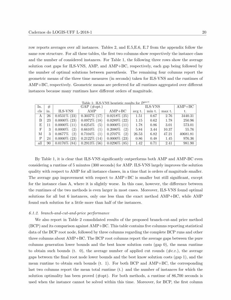
results are summarized in Table 1. In this table, besides the headers, each row reports average
results for one of the six instance classes of the corresponding classical CVRP benchmark. The last
Cadernos do LOGIS-UFF L-2018-1 20
row reports averages over all instances. Tables 2, and E.5,E.6, E.7 from the appendix follow the
same row structure. For all these tables, the first two columns show respectively the instance class
and the number of considered instances. For Table 1, the following three rows show the average
solution cost gaps for ILS-VNS, AMP, and AMP+BC, respectively, each gap being followed by
the number of optimal solutions between parenthesis. The remaining four columns report the
geometric means of the three time measures (in seconds) taken for ILS-VNS and the runtimes of
AMP+BC, respectively. Geometric means are preferred for all runtimes aggregated over different
instances because many runtimes have different orders of magnitude.
Table 1: ILS-VNS heuristic results for Dpart
In. # GAP (#opt.) ILS-VNS AMP+BCcls in. ILS-VNS AMP AMP+BC avg t. min t. max t. t.A 26 0.0531% (23) 0.3037% (17) 0.0218% (25) 1.51 0.67 2.76 3440.31B 23 0.0000% (23) 0.0972% (18) 0.0289% (22) 1.15 0.62 1.78 250.96E 11 0.0000% (11) 0.6254% (5) 0.0000% (11) 1.78 0.86 3.01 573.01F 3 0.0000% (2) 0.6610% (1) 0.2080% (2) 5.84 3.44 10.37 55.76M 3 0.0677% (2) 0.7104% (1) 0.2707% (2) 26.53 6.82 47.21 40681.81P 24 0.0000% (23) 0.2122% (14) 0.0000% (23) 0.86 0.48 1.45 976.36
all 90 0.0176% (84) 0.2913% (56) 0.0296% (85) 1.42 0.71 2.41 981.90
By Table 1, it is clear that ILS-VNS significantly outperforms both AMP and AMP-BC even
considering a runtime of 5 minutes (300 seconds) for AMP. ILS-VNS largely improves the solution
quality with respect to AMP for all instance classes, in a time that is orders of magnitude smaller.
The average gap improvement with respect to AMP+BC is smaller but still significant, except
for the instance class A, where it is slightly worse. In this case, however, the difference between
the runtimes of the two methods is even larger in most cases. Moreover, ILS-VNS found optimal
solutions for all but 6 instances, only one less than the exact method AMP+BC, while AMP
found such solution for a little more than half of the instances.
6.1.2. branch-and-cut-and-price performance
We also report in Table 2 consolidated results of the proposed branch-cut-and price method
(BCP) and its comparison against AMP+BC. This table contains five columns reporting statistical
data of the BCP root node, followed by three columns regarding the complete BCP runs and other
three columns about AMP+BC. The BCP root columns report the average gaps between the pure
columns generation lower bounds and the best know solution costs (gap 0), the mean runtime
to obtain such bounds (t. 0), the average number of applied cut rounds (#c.r.), the average
gaps between the final root node lower bounds and the best know solution costs (gap 1), and the
mean runtime to obtain such bounds (t. 1). For both BCP and AMP+BC, the corresponding
last two columns report the mean total runtime (t.) and the number of instances for which the
solution optimality has been proved (#opt). For both methods, a runtime of 86,700 seconds is
used when the instance cannot be solved within this time. Moreover, for BCP, the first column

Cadernos do LOGIS-UFF L-2018-1 21
gives the average number of branch-and-cut-and-price nodes (#n.), and for AMP-BC, the first
column gives the final gap between the obtained lower bound and the best known solution cost
(gap).
Table 2: branch-and-cut-and-price results for Dpart
In. # BCP root BCP AMP+BCcls in. gap 0 t. 0 #c.r. gap 1 t. 1 #n. t. #opt. gap t. #opt.A 26 2.16% 0.70 3.7 0.00% 2.91 1.00 2.91 26 1.97% 3440.31 12B 23 3.68% 1.31 2.8 0.01% 5.95 1.05 5.98 23 1.39% 250.96 13E 11 2.31% 2.79 5.4 0.00% 11.40 1.00 11.40 11 2.19% 573.01 5F 3 3.01% 139.10 5.0 0.30% 309.40 5.37 833.42 2 1.10% 55.76 2M 3 1.66% 12.49 14.7 0.20% 52.44 3.33 153.51 3 2.70% 40681.81 1P 24 1.27% 0.51 2.8 0.00% 1.47 1.00 1.48 24 2.09% 976.36 10
all 90 2.34% 1.17 3.9 0.02% 4.43 1.11 4.75 89 1.87% 981.90 43
By Table 2, it can be seen that the proposed BCP outperforms AMP+BC for all instance
classes except F, where both methods solve two out of three instances having 44, 71 and 134
customers. In this case, the two smaller instances are harder for BCP because they have relatively
long routes. Overall, BCP solves all instances but one while less than half of them are solved
by AMP+BC. Although the only open instance has been tried for more than 24 hours without
success, all other instances have been solved in less than 2 hours (7,200 seconds). Note that the
mean runtime of BCP is two orders of magnitude smaller than that of AMP+BC. It is worth
to mention that BCP used the solution cost found by ILS-VNS as an initial upper bound (we
have used an upper bound one unit larger for all instances with up to 120 customers for testing
purposes). However, it can be seen in Table 1 that adding the heuristic time to the total BCP
time would not change much the results. It is also remarkable from Table 2 that the cuts closed
almost all the gap left by the column generation lower bound, which allows us to solve almost
all instances at the root node. Note however that the root node for BCP includes the resolution
of IP problems generated through the enumeration of all useful elementary routes by CPLEX,
when such problems are small enough. Nevertheless, the root lower bound used to compute the
numbers in the column gap 1 does not include this resolution step.
6.1.3. Preprocessing
Applying the pre-processing detailed in Section 2.3, we could remove nearly 80% of the sub-
problems, and 22 of 90 instances were reduced to deterministic homogeneous CVRP (with one
subproblem). Further details are provided in Section Appendix E.1.1 of the appendix.
6.1.4. New capacity cuts
The literature cuts are already very effective, closing more than 60% of the gap. Yet, the new
cuts close 33% of the remaining gap, which is a significant improvement. We refer to Section Ap-
pendix E.2 of the appendix for details.
Cadernos do LOGIS-UFF L-2018-1 22
6.2. Experiments for Dcard
6.2.1. New Instances
The new instances are also derived from the classical CVRP instances. As the uncertainty set
Dcard makes the problem harder, the considered 90 instances ranges from 12 to 120 customers (we
included the instances E-n13-k4 and A-n45-k7 not present in the Dpart data set and removed the
largest F-n135-k7 and M-n151-k12). The additional data required to the robust counterpart has
been generated based on the following three parameters: µ is the relative magnitude of demand
deviations, ρ is the multiplicative factor applied to the average route length to compute the
value of Γ, and τ is proportional to the difference between the vehicle capacity and the minimum
required to make the instance feasible, where the scale factor applied makes τ equal to one if
the capacity is the minimum required to use m − 1 vehicles. Smaller values of τ lead to tighter
capacities. Further details on the generation of the specific robust counterpart parameters are
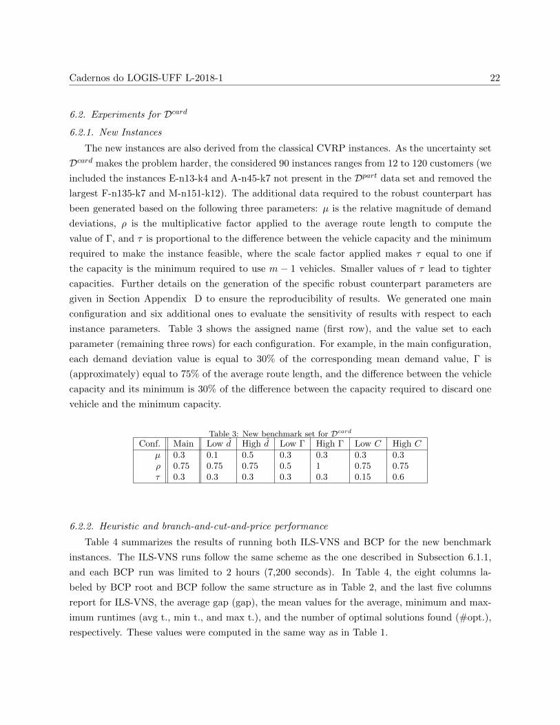
given in Section Appendix D to ensure the reproducibility of results. We generated one main
configuration and six additional ones to evaluate the sensitivity of results with respect to each
instance parameters. Table 3 shows the assigned name (first row), and the value set to each
parameter (remaining three rows) for each configuration. For example, in the main configuration,
each demand deviation value is equal to 30% of the corresponding mean demand value, Γ is
(approximately) equal to 75% of the average route length, and the difference between the vehicle
capacity and its minimum is 30% of the difference between the capacity required to discard one
vehicle and the minimum capacity.
Table 3: New benchmark set for Dcard
Conf. Main Low d High d Low Γ High Γ Low C High Cµ 0.3 0.1 0.5 0.3 0.3 0.3 0.3ρ 0.75 0.75 0.75 0.5 1 0.75 0.75τ 0.3 0.3 0.3 0.3 0.3 0.15 0.6
6.2.2. Heuristic and branch-and-cut-and-price performance
Table 4 summarizes the results of running both ILS-VNS and BCP for the new benchmark
instances. The ILS-VNS runs follow the same scheme as the one described in Subsection 6.1.1,
and each BCP run was limited to 2 hours (7,200 seconds). In Table 4, the eight columns la-
beled by BCP root and BCP follow the same structure as in Table 2, and the last five columns
report for ILS-VNS, the average gap (gap), the mean values for the average, minimum and max-
imum runtimes (avg t., min t., and max t.), and the number of optimal solutions found (#opt.),
respectively. These values were computed in the same way as in Table 1.

Cad
ernos
do
LO
GIS
-UF
FL
-2018-1
23Table 4: Heuristic and branch-and-cut-and-price results for Dcard
# BCP root BCP ILS-VNSIn. cls in. gap 0 t. 0 #c. gap 1 t. 1 #n. t. #opt. gap avg t. min t. max t. #opt.
A 27 2.19% 2.50 4.4 0.02% 17.88 1.11 18.81 27 0.03% 1.98 0.76 4.14 24B 23 5.14% 3.44 5.9 0.23% 41.48 1.50 69.54 20 0.00% 2.57 1.01 5.04 19E 13 1.91% 5.69 5.3 0.03% 24.84 1.16 27.79 13 0.12% 2.85 1.07 4.97 10F 2 2.00% 154.53 0.5 0.00% 222.81 1.00 222.83 2 0.00% 1.26 1.20 1.33 2M 2 4.03% 39.31 6.5 0.00% 108.21 1.00 108.23 2 0.00% 5.72 2.87 10.53 2P 23 1.59% 2.28 3.4 0.00% 10.74 1.00 10.75 23 0.00% 1.93 0.74 3.85 23
all 90 2.79% 3.48 4.6 0.07% 22.47 1.17 26.47 87 0.03% 2.25 0.89 4.37 80
Low d 90 2.79% 3.80 4.3 0.03% 26.14 1.13 28.60 89 0.00% 2.37 0.82 4.67 87
High d 90 2.68% 3.36 4.9 0.16% 19.69 1.35 25.84 86 0.02% 3.50 0.94 7.14 82Low Γ 90 2.74% 4.28 5.4 0.10% 27.71 1.20 30.97 89 0.01% 2.99 1.04 5.65 81High Γ 90 2.67% 2.66 4.6 0.07% 14.77 1.17 17.20 87 0.02% 2.53 0.86 5.02 81Low C 90 3.10% 3.79 6.5 0.43% 26.89 1.37 34.40 85 0.13% 6.10 1.46 13.58 69High C 90 2.92% 3.83 4.6 0.18% 23.91 1.41 33.80 84 0.01% 1.95 0.85 3.35 80

Cadernos do LOGIS-UFF L-2018-1 24
By Table 4, it can be seen that the overall performance of the proposed methods for the
new benchmark set is roughly similar to that observed for the literature instances: ILS-VNS
can find the great majority of the optimal solutions in a few seconds, most of the gap left by
the column generation lower bound is closed but the combination of the proposed cuts with the
literature cuts previously proposed for the deterministic version, and only a few instances could
not be solved exactly withing two hours of runtime. A more detailed analysis however reveals
that there are some cases where instances can still be challenging for the proposed algorithms.
For instance, ILS-VNS could not find optimal solutions for 21 out of 90 low-capacity instances
and the average gap with respect to the best-known solutions is more than four times the gap of
any other configuration. We observed that this is because it is harder to find feasible solutions
with this configuration and the proposed method is not prepared to handle that. Moreover, for
the main class, the three instances that could not be solved belong to the class B, having 50,
56 and 63 customers. It is worth mentioning that four larger instances of the same class could
be solved relatively easily. The main reason for not solving such instances is that all of them
have root gaps larger than 1.5%, which is more than 20 times larger than the average gap for the
whole benchmark set in the main configuration. Regarding other configurations, it can be seen
the instances with lower demand deviations are easier for both ILS-VNS and BCP in the sense
that more optimal solutions are found by the heuristics, more instances could be solved exactly,
and both the root gaps of BCP and the gaps of ILS-VNS with respect to the best known solution
are smaller. We also observe that the root gaps of BCP are significantly larger for high demand
deviations, and for both higher and lower capacities, in the latter case being more than six times
larger than in the main configuration. For the lower capacity, we observed that the higher root
gap is compensated by the stronger effect of fixing by reduced cost and enumeration in these
instances, which leads to a number of solved instances than is not very much different from the
main configuration. Overall, only 23 out of 630 instances could not be solved exactly within 2
hours, ranging from 50 to 100 customers, where 18 of them are from the class B, 4 are from the
class E and 1 is from the class A.
6.2.3. Effect of approximate feasibility testing
We have also measured the effect of the proposed approximate feasibility checking procedure.
For that, we measured the average runtime for each instance with this technique disable and
enabled. The average ratio between the two times is 2.7 for the main configuration. For separate
instance classes, this average ratio does not change much except for the classes F and M, which
are 1.66 and 3.68, respectively. For more detailed results, we refer to Section Appendix E.3 on
the appendix.
6.2.4. Preprocessing
The number of pricing problems left after the preprocessing is roughly 15% smaller than before,
see Section Appendix E.1.2 of the appendix for details.

Cadernos do LOGIS-UFF L-2018-1 25
6.2.5. New capacity cuts
The literature cuts close 40% of the gap for these instances, and the new ones close nearly
40% of the remaining gap, see Section Appendix E.2 of the appendix.
7. Conclusion
Modern branch-and-cut-and-price algorithms have solved vehicle routing instances larger and
faster than ever before. In this work, we carry over these techniques to the robust capacitated
vehicle routing problems with knapsack uncertainty. Extending existing results in robust com-
binatorial optimization and providing original reduction strategies, new valid inequalities, and
improved primal heuristics we are able to solve all but one instance proposed by Gounaris et al.
(2013) for the partition polytope, while obtaining very good results for the new instances gener-
ated for the budget polytope.
Future work could seek to extend these good numerical results to other variants of robust
vehicle routing problems, such as the one involving time windows and uncertain travel times.
Yet, the later problem facing a strongly NP-hard pricing problem in the robust case (Pessoa
et al. 2015), its efficient solution would require more than a simple extension of the techniques
presented in this work (however, if travel times are deterministic, the extension is straightforward).
Further extensions could also apply the present decomposition approach to other combinatorial
optimization problems with uncertainty in the binary knapsack substructure, such as the bin
packing problem with item size uncertainty (Song et al. 2018).
References
Aissi H, Bazgan C, Vanderpooten D (2009) Min-max and min-max regret versions of combinatorial opti-
mization problems: A survey. European Journal of Operational Research 197(2):427–438.
Alvarez-Miranda E, Ljubic I, Toth P (2013) A note on the bertsimas & sim algorithm for robust combina-
torial optimization problems. 4OR 11(4):349–360.
Baldacci R, Christofides N, Mingozzi A (2008) An exact algorithm for the vehicle routing problem based
on the set partitioning formulation with additional cuts. Mathematical Programming 115:351–385.
Baldacci R, Mingozzi A, Roberti R (2011) New route relaxation and pricing strategies for the vehicle
routing problem. Operations Research 59(5):1269–1283.
Ben-Tal A, El Ghaoui L, Nemirovski A (2009) Robust optimization (Princeton University Press).
Ben-Tal A, Goryashko AP, Guslitzer E, Nemirovski A (2004) Adjustable robust solutions of uncertain
linear programs. Math. Program. 99(2):351–376.
Ben-Tal A, Nemirovski A (1998) Robust convex optimization. Math. Oper. Res. 23(4):769–805.
Bertsimas D, Sim M (2003) Robust discrete optimization and network flows. Math. Program. 98(1-3):49–71.
Bertsimas D, Sim M (2004) The price of robustness. Operations Research 52(1):35–53.
Birge JR, Louveaux FV (2011) Introduction to Stochastic programming (2nd edition) (Springer Verlag).
Cadernos do LOGIS-UFF L-2018-1 26
Bulhoes T, Sadykov R, Uchoa E (2018) A branch-and-price algorithm for the minimum latency problem.
Computers & Operations Research 93:66–78.
Dinh T, Fukasawa R, Luedtke J (2018) Exact algorithms for the chance-constrained vehicle routing problem.
Mathematical Programming In press.
Fukasawa R, Longo H, Lysgaard J, Aragao MPd, Reis M, Uchoa E, Werneck RF (2006) Robust branch-and-
cut-and-price for the capacitated vehicle routing problem. Mathematical Programming 106(3):491–
511.
Gendreau M, Laporte G, Seguin R (1996) Stochastic vehicle routing. Eur. J. Oper. Res. 88(1):3–12.
Ghosal S, Wiesemann W (2018) The distributionally robust chance constrained vehicle routing problem.
URL www.optimization-online.org/DBHTML/2018/08/6759.html.
Goetzmann K, Stiller S, Telha C (2011) Optimization over integers with robustness in cost and few con-
straints. WAOA 2011, Saarbrucken, Germany, September 8-9, 2011, Revised Selected Papers, 89–101.
Gounaris CE, Repoussis PP, Tarantilis CD, Wiesemann W, Floudas CA (2016) An adaptive memory
programming framework for the robust capacitated vehicle routing problem. Transp. Sci. 50(4):1239–
1260.
Gounaris CE, Wiesemann W, Floudas CA (2013) The robust capacitated vehicle routing problem under
demand uncertainty. Operations Research 61(3):677–693.
Irnich S, Desaulniers G (2005) Shortest Path Problems with Resource Constraints, 33–65 (Boston, MA:
Springer US).
Irnich S, Desaulniers G, Desrosiers J, Hadjar A (2010) Path-reduced costs for eliminating arcs in routing
and scheduling. INFORMS Journal on Computing 22(2):297–313.
Jepsen M, Petersen B, Spoorendonk S, Pisinger D (2008) Subset-row inequalities applied to the vehicle-
routing problem with time windows. Operations Research 56(2):497–511.
Kouvelis P, Yu G (2013) Robust discrete optimization and its applications, volume 14 (Springer Science &
Business Media).
Laporte G, Nobert Y (1983) A branch and bound algorithm for the capacitated vehicle routing problem.
Operations-Research-Spektrum 5(2):77–85.
Lee C, Lee K, Park K, Park S (2012) Technical note - branch-and-price-and-cut approach to the robust
network design problem without flow bifurcations. Operations Research 60(3):604–610.
Lee T, Kwon C (2014) A short note on the robust combinatorial optimization problems with cardinality
constrained uncertainty. 4OR 12(4):373–378.
Lysgaard J, Letchford AN, Eglese RW (2004) A new branch-and-cut algorithm for the capacitated vehicle
routing problem. Mathematical Programming 100(2):423–445.
Ordonez F (2010) Robust vehicle routing. TUTORIALS in Operations Research 153–178.
Pecin D, Pessoa A, Poggi M, Uchoa E, Santos H (2017a) Limited memory rank-1 cuts for vehicle routing
problems. Operations Research Letters 45(3):206 – 209.
Pecin D, Pessoa AA, Poggi M, Uchoa E (2017b) Improved branch-cut-and-price for capacitated vehicle
routing. Math. Program. Comput. 9(1):61–100.
Penna PHV, Subramanian A, Ochi LS (2013) An iterated local search heuristic for the heterogeneous fleet
vehicle routing problem. Journal of Heuristics 19(2):201–232.

Cadernos do LOGIS-UFF L-2018-1 27
Pessoa A, Sadykov R, Uchoa E, Vanderbeck F (2018) Automation and combination of linear-programming
based stabilization techniques in column generation. INFORMS Journal on Computing 30(2):339–
360.
Pessoa AA, Pugliese LDP, Guerriero F, Poss M (2015) Robust constrained shortest path problems under
budgeted uncertainty. Networks 66(2):98–111.
Poss M (2013) Robust combinatorial optimization with variable budgeted uncertainty. 4OR 11(1):75–92.
Poss M (2014) Robust combinatorial optimization with variable cost uncertainty. EJOR 237(3):836–845.
Poss M (2018) Robust combinatorial optimization with knapsack uncertainty. Dis. Opt. 27:88–102.
Righini G, Salani M (2006) Symmetry helps: Bounded bi-directional dynamic programming for the ele-
mentary shortest path problem with resource constraints. Discrete Optimization 3(3):255 – 273.
Sadykov R, Uchoa E, Pessoa A (2017) A bucket graph based labeling algorithm with application to vehicle
routing. Cadernos do LOGIS L-2017-7, UFF, URL http://www2.logis.uff.br/cadernos/.
Song G, Kowalczyk D, Leus R (2018) The robust machine availability problem – bin packing under uncer-
tainty. IISE Transactions In Press.
Sungur I, Ordonez F, Dessouky M (2008) A robust optimization approach for the capacitated vehicle
routing. IIE Transactions 40(5):509–523.
Tadayon B, Smith JC (2015) Algorithms and complexity analysis for robust single-machine scheduling
problems. J. Scheduling 18(6):575–592.
Talla Nobibon F, Leus R (2014) Complexity results and exact algorithms for robust knapsack problems.
J. Optim. Theory Appl. 161(2):533–552.
Uchoa E, Fukasawa R, Lysgaard J, Pessoa AA, de Aragao MP, Andrade D (2008) Robust branch-cut-and-
price for the capacitated minimum spanning tree problem over a large extended formulation. Math.
Program. 112(2):443–472, URL http://dx.doi.org/10.1007/s10107-006-0043-y.
Vidal T, Crainic TG, Gendreau M, Prins C (2013) Heuristics for multi-attribute vehicle routing problems:
A survey and synthesis. European Journal of Operational Research 231(1):1 – 21.
Vidal T, Crainic TG, Gendreau M, Prins C (2014) A unified solution framework for multi-attribute vehicle
routing problems. European Journal of Operational Research 234(3):658 – 673.
Wiesemann W, Kuhn D, Sim M (2014) Distributionally robust convex optimization. Oper. Res. 62(6):1358–
1376.
Appendix A. Missing proofs
Appendix A.1. Proof of Theorem 1
Let us first prove⋃θ∈Θ
Y knapθ ⊆ Y knap. Hence, let y ∈ Y knap, and ξ∗ ∈ argmax
ξ∈Ξ
{n∑i=1
diwiξiyi
}.
By the strong duality of linear programming, we have that
b>θ∗ + (dθ∗)>y = d
>y + b>θ∗ + w>z∗ = d
>y +
n∑i=1
diwiξ∗i yi ≤ C,
where the last inequality holds because y ∈ Y knap. Thus, y ∈ Y knapθ∗ .

Cadernos do LOGIS-UFF L-2018-1 28
To prove the reverse inclusion, let y ∈ Y knapθ′ for some θ′ ∈ Θ. We have that
d>y + max
ξ∈Ξ
{n∑i=1
diwiξiyi
}=
d>y + min
θ∈IRs+
{b>θ +
n∑i=1
max{0, di − wiθk(i)} yi
}≤
d>y + b>θ′ +
n∑i=1
max{0, di − wiθ′k(i)} yi =
b>θ′ + (dθ′)>y ≤ C.
As a result, y ∈ Y knap, finishing the proof.
Appendix A.2. Proof of Theorem 3
Clearly,⋃
θ∈Θ∗Y knapθ ⊆
⋃θ∈Θ∗
Y knapθ = Y knap. Hence, we prove below that Y knap ⊆
⋃θ∈Θ∗
Y knapθ .
For that, let y ∈ Y knap, and ξ∗ ∈ argmaxξ∈Ξ
{n∑i=1
diwiξiyi
}. Assume also that ξ∗ is an extreme
solution, meaning that for all i, j ∈ {1, . . . , n} with i 6= j, ξ∗i , ξ∗j > 0, and k(i) = k(j), either
ξ∗i = wi or ξ∗j = wj . Note that a non-extreme solution may only be optimal if diwiyi =
djwjyj
for all i, j ∈ {1, . . . , n} with i 6= j, ξ∗i , ξ∗j > 0, k(i) = k(j), ξ∗i < wi, and ξ∗j < wj . For each
k ∈ {1, . . . , s}, let I∗k = {i ∈ Vk | ξ∗i > 0}, I∗k = {i ∈ Vk | ξ∗i = wi}. We further assume w.l.o.g.
that ξ∗i > 0 =⇒ yi = 1 since letting ξ∗i > 0 for some i with yi = 0 does not help to increase the
left-hand side of (2). Let also (θ∗, z∗) be an optimal solution to the left-hand side of (3), where
the value of z∗i is set as max{0, diwi yi − θ∗k(i)} for i = 1, . . . , n.
It remains to prove that y also satisfies
∑i∈Vk
di>wiθ∗k
wiyi ≤ bk ≤∑i∈Vk
di≥wiθ∗k
wiyi, ∀k ∈ {1, . . . , s} | θ∗k > 0, (A.1)
and
∑i∈Vk
wiyi ≤ bk, ∀k ∈ {1, . . . , s} | θ∗k = 0. (A.2)
For that, we use the complementary slackness of the solutions ξ∗ and (θ∗, z∗), as they are
optimal to a linear programming problem and its dual, respectively. Namely, we have that
θ∗k > 0 =⇒∑i∈Vk
ξ∗i = bk,
for k = 1, . . . , s, and,

Cadernos do LOGIS-UFF L-2018-1 29
ξ∗i > 0 =⇒ z∗i + θ∗k(i) =diwiyi,
for i = 1, . . . , n. Given this fact, the second inequality of (A.1) holds because, since ξ∗i ≤ wi for
all i ∈ I∗k , and ξ∗i = 0 for all i ∈ I∗k \ Vk, we have that
bk =∑i∈Vk
ξ∗i ≤∑i∈I∗k
wi ≤∑i∈Vk
di≥wiθk
wiyi,
where the last inequality holds because both ξ∗i > 0 and z∗i + θ∗k(i) = diwiyi together imply that
di ≥ wiθ∗k(i). For the first inequality of (A.1), we have that
bk =∑i∈Vk
ξ∗i ≥∑i∈I∗k
wiyi ≥∑i∈Vk
di>wiθ∗k
wiyi,
where the first inequality holds by definition of I∗k , and the second one is true because both yi = 1
and di > wiθ∗k(i) together imply that z∗i > 0, which implies by complementary slackness between
ξ∗ and (θ∗, z∗) that ξ∗i = wi. Finally, (A.2) is also true because, since ξ∗ is an optimal solution
to the left-hand side of (2) and∑i∈Vk
ξ∗i < bk, we have that ξ∗i = wi for all i ∈ Vk with yi = 1 when
θ∗k = 0.
Appendix A.3. Proof of Theorem 4
In order to be able to prove the theorem, we define a new optimization problem that turns out
to be a relaxation of the problem of assigning the vertices of S to the minimum number of routes,
respecting the vehicle capacities for demands in Dpart = {d = d+ ξ |∑i∈Vk
ξi ≤ bk, k = 1, . . . , s, ξ ≤
κd}. We call it the Stripe Crossing Problem (SCP).
In SCP, we are given s striped boards, where board k has height qk(S), for k = 1, . . . , s.
Each board k has alternated gray and white horizontal stripes, the lowest one being gray. All
gray stripes in board k have height bkκ , and all its white stripes have height max{0, C − 1+κ
κ bk},for k = 1, . . . , s. Only the highest stripe may have a truncated height if it does not fit into the
remaining board space. Note that board k is completely gray if C ≤ 1+κκ bk. SCP asks for a
way to draw vertical lines crossing all stripes of all boards, from bottom to top, minimizing the
number of used pens. It is assumed that each pen has a limited amount C of ink, and spends 1
and 1 + κ units of ink per line length unit in white and gray stripes, respectively. Moreover, each
pen is allowed to draw at most one contiguous line segment in each board. Figure A.1 illustrates
SCP by depicting an instance with 3 boards and a solution using 6 pens. The stripe heights of
board 1 and the height of board 3 are indicated in the figure. Drawn lines are represented as wide
dark-gray vertical lines with the corresponding pen indicated on the right.

Cadernos do LOGIS-UFF L-2018-1 30
< b1κ
C − 1+κκ b1
b1κ
b1κ
C − 1+κκ b1
PEN 1
PEN 2
PEN 3
PEN 4
PEN 5PEN 3
PEN 6
BOARD 1 BOARD 2 BOARD 3
q3(S)
PEN 1
Figure A.1: A Stripe Crossing Problem instance.
Next, we present two propositions that demonstrate the link between SCP and the minimum
number of vehicles required to serve all customers in a given set S.In this link, boards represent
partitions, pens represent vehicles, gray stripes represent demands that deviate in a gives scenario,
and white stripes represent demands that do not deviate from their mean values. We also give an
additional proposition proving that the newly proposed inequality strictly dominates (24).
Proposition 3. The total line length drawn with a given pen over the gray stripes of a given
board is at most bkκ .
Proof. If C ≤ 1+κκ bk, the proposition holds because the pen spends 1 + κ ink per length unit,
being limited to a total length of C1+κ ≤
bkκ . Otherwise, suppose that a given pen draws a line
length ` > bkκ over the gray stripes of a board k. Since the height of any gray stripe in this board
is not greater than bkκ , the pen has to cross one of its white stripes completely. For that, it must
spend at least C − 1+κκ bk + (1 + κ)` > C, which contradicts the limit on the amount of available
ink for this pen, finishing the proof.
Proposition 4. The optimal solution r∗(S) of SCP is a lower bound on the number of routes
required to serve all customers in S in the robust CVRP with the uncertainty set Dpart.
Proof. Let y be a variable matrix representing a feasible solution for the robust CVRP with Dpart,where y`i = 1 if vertex i ∈ V 0 is served by route ` ∈ {1, . . . ,m}, and 0 otherwise. We assume
w.l.o.g. that routes ` = 1, . . . , r, and only them, visit S. Then, it is enough to prove that there is
a feasible solution to the corresponding SCP instance using r pens.
Associate each pen to a route `, for ` = 1, . . . , r. Then, for each board k, build a crossing
vertical line by concatenating line segments drawn by all pens, such that the length of the line
segment drawn by pen ` is given by∑
i∈S∩Vkdiy`i. Note that the total line length drawn over the
board k is given byr∑=1
∑i∈S∩Vk
diy`i = qk(S) since all the demand of S is served by the r routes.
Now, let α`k and β`k be the total line length drawn by pen ` over the white and the gray stripes
of board k, respectively, for k = 1, . . . , s, and ` = 1, . . . , r. We have that the total ink spent by

Cadernos do LOGIS-UFF L-2018-1 31
each pen ` is given by
s∑k=1
(α`k + (1 + κ)β`k) =s∑
k=1
((α`k + β`k) + κβ`k)
≤s∑
k=1
∑i∈S∩Vk
diy`i + κmin
bkκ , ∑i∈S∩Vk
diy`i
≤s∑
k=1
∑i∈Vk
diy`i + min
bk,∑i∈Vk
κdiy`i
= maxd∈Dpart
∑i∈V 0
diy`i
≤ Cwhere the first inequality is a consequence of Proposition 3, and the last one holds because ` is
a feasible route for the robust CVRP. Hence, the constructed solution is feasible for the SCP
instance, finishing the proof.
We are now able to prove the main result of this section.
Proof. of Theorem 4
Proof. First, we show that γk is the exact line length drawn contiguously by a pen with ink C over
the board k if it is used exclusively in this board. To see this, note that, for C ≤ 1+κκ bk, where
board k is completely gray, γk = C1+κ gives the exact length that can be drawn by a pen with ink
C over a gray area. Otherwise, when C > 1+κκ bk, a pen with ink C spends 1+κ
κ bk drawing a total
length of bkκ over the gray stripes, and the remaining ink to draw a total length of C− 1+κ
κ bk over
the white stripes. The sum of these lengths is exactly γk = C − bk.Now, note that
⌊qk(S)γk
⌋is the number of times a pen becomes empty when crossing a board
k (assuming that all pens used in this board are not used elsewhere). Moreover, qk(S) is the
remaining height of board k after excluding the part crossed by these pens. Given that, the exact
total ink required to cross board k can be expressed as
C
⌊qk(S)
γk
⌋+ qk(S) + κmin
{bkκ, qk(S)
},
for k = 1 . . . , s. Thus, summing it up for all boards, dividing by C, and rounding the result up
gives a lower bound on r∗(S) which is exactly equal to r(S). Hence, by Proposition 4, r(S) is a
valid lower bound on the left-hand side of (4) for any feasible robust CVRP solution.

Cadernos do LOGIS-UFF L-2018-1 32
Appendix A.4. Proof of Proposition 1
Note that, for the particular case considered here, r(S) can be rewritten ass∑
k=1
(qk(S) + min{bk, κ qk(S)})
C
,and
r(S) =s∑
k=1
∑i∈S∩Vk
minθ∈{0,ek}
dθiC − b>θ
=s∑
k=1
∑i∈S∩Vk
min
{(1 + κ)di
C,
diC − bk
}
=
s∑k=1
min
{1 + κ
C,
1
C − bk
}qk(S)
=
s∑k=1
1
C
(qk(S) + min
{κ,
bkC − bk
}qk(S)
),
where ek represents a vector with the kth component equal to one, and all remaining ones equal to
zero. The first equality holds because the minimum ofdθi
C−b>θ over Θ (here assumed to be equal to
Θ) is always achieved when θ` = 0 for all ` 6= k. Hence, to prove that r(S) ≥ max{dr(S)e, r(S)},it is sufficient to show that
C
⌊qk(S)
γk
⌋+ qk(S) + min{bk, κ qk(S)}
≥ max
{qk(S) + min{bk, κ qk(S)}, qk(S) + min
{bk
C − bk, κ
}qk(S)
},
or, equivalently, that
C
⌊qk(S)
γk
⌋+ qk(S) + min {bk, κ qk(S)} (A.3)
≥ qk(S) + min
{max
{1,
qk(S)
C − bk
}bk, κ qk(S)
}, (A.4)
for k = 1, . . . , s.
We divide into two cases. First, assume that C1+κ ≥ C − bk. This implies that
γk =C
1 + κ, (A.5)
and also that bkκ ≥
C1+κ = γk. Moreover, by definition of qk(S), it is smaller than γk. Hence,

Cadernos do LOGIS-UFF L-2018-1 33
we have that
bk > κ qk(S).
Applying this result, the definition of qk(S), and (A.5) to (A.3) gives the expression
C
⌊qk(S)
γk
⌋+ (1 + κ)
(qk(S)− C
1 + κ
⌊qk(S)
γk
⌋)= (1 + κ)qk(S),
which is greater than or equal to (A.4).
Now, it remains to prove it for the case where C1+κ < C − bk = γk, which implies that
C < (C − bk) + κγk
bk < κγk. (A.6)
In this case, we may rewrite (A.3) as
C
⌊qk(S)
γk
⌋+ qk(S)− (C − bk)
⌊qk(S)
γk
⌋+ min
{bk, κ qk(S)− κ γk
⌊qk(S)
γk
⌋}= qk(S) + min
{(⌊qk(S)
γk
⌋+ 1
)bk, κ qk(S) + (bk − κ γk)
⌊qk(S)
γk
⌋},
which can be shown to be greater than or equal to (A.4) by applying (A.6).
To show that the inequality can be strict, we extend Example 3 by including the customers
5 and 6 in S ∩ V2, with d5 = d6 = d5 = d6 = 2. In this case, r(S) remains equal to 2 because
the deviation considered for partition 2 in already in its maximum, and the total demand to be
served, including these deviations, increases from 7 to only 11 < 2C. Moreover, r(S) increases
byd
(0,1)5C−2 +
d(0,1)6C−2 = 1, becoming also equal to 2. However, r(S) = 3 since γ2 = 4, q2(S) = 8, and
q1(S) = 1.
Appendix A.5. Proof of Proposition 2
It is enough to prove that there exists ξ ∈ Ξ such thatp∑=1
di`ξi` +|r′|∑
`=q+1
dj`ξj` = d(r′′). For
that, we use the fact that ξ∗ is the worst-case scenario for both r and r′. Clearly, if Γ1 + Γ2 ≤ Γ
the proposition holds since d(r′′) =p∑=1
di`ξ∗i`
+|r′|∑
`=q+1
dj`ξ∗j`
. Next, we prove that it also holds only
for Γ1 + Γ2 > Γ and d1 ≥ d2, since the remaining case is analogous. For that, let
ξ` =
{Γ−Γ1
Γ2ξ∗` if ` ∈ {jq+1, . . . , j|r′|}
ξ∗` otherwise.
Clearly ξ ∈ Ξ. Moreover, since|r′|∑
`=q+1
dj` ξj` = (Γ− Γ1)|r′|∑
`=q+1
dj`ξ∗j`
Γ2= (Γ− Γ1)d2, we have that

Cadernos do LOGIS-UFF L-2018-1 34
p∑=1
di` ξi` +|r′|∑
`=q+1
dj` ξj` = d(r′′), completing the proof.
Appendix B. Three examples for the new capacity cuts
To simplify the cut strength analysis that follows, we assume from now on that Θ = Θ. The
first two examples look at the case D = Dcard.
Example 1. Consider that S = {1, . . . , 20}, Γ = 1, C = 3, and d1 = · · · = d20 = d1 = · · · = d20 =
1. In this case, since only one deviation is allowed for all d ∈ D, we obtain that r(S) = d21/3e = 7.
Alternatively, since Θ = {0, 1}, we have that r(S) = 20 min{2/3, 1/2} = 10.
Although r(S) is usually much larger than r(S) when the number of routes required to serve
S is large, the next example shows that the opposite scenario may occur if only two routes are
required.
Example 2. Consider S = {1, . . . , 5}, Γ = 3, C = 15, d1 = d1 = 5, and d2 = · · · = d5 = d2 =
· · · = d5 = 1. In this case, since the total demand to be served in S can reach 16 > C (by deviating
d1, d2, and d3, for example), we obtain that r(S) = 2. However, since Θ = {0, 1}, we have that
r(S) = min{10/15, 9/12}+ 4 min{2/15, 1/12} = 1.
Note that Example 1 can be easily adapted for D = Dpart because all deviations are unitary.
For that, it is enough to assume that all customers in S belong to the same partition Vk of V 0, and
that bk = Γ = 1. This shows that r(S) can also be strictly larger than r(S) for the uncertainty
set proposed in Gounaris et al. (2013). It is worth mentioning that all deviations in this example
are proportional to the corresponding mean demand values, which is an assumption of the special
case addressed by Theorem 4. The third example shows that the opposite strict inequality may
also occur regardless of whether deviations are proportional to mean values or not.
Example 3. In this case, assume that V 0 is partitioned into two sets (s = 2), S = {1, 2, 3, 4},and S ∩V1 = {1}. Moreover, we have C = 6, d1 = · · · = d4 = d1 = · · · = d4 = 1, and b1 = b2 = 2.
In this case, note that r(S) = 2 since the total deviation of d2, d3, and d4 can reach the limit of
the partition 2, and d1 can deviate by one unity since it is in another partition, resulting in a total
demand of 7 > C units to be served. However, since Θ = {(0, 0), (0, 1), (1, 0), (1, 1)}, we have
r(S) =d
(1,0)1
C − 2+d
(0,1)2
C − 2+d
(0,1)3
C − 2+d
(0,1)4
C − 2= 1.
Appendix C. Further algorithmic details
Appendix C.1. Separation of capacity cuts
Let x be a fractional solution to RVRP-2IF. In our implementation, we separate robust ca-
pacity inequalities (24) at each node of the branch-and-bound tree using the heuristic described
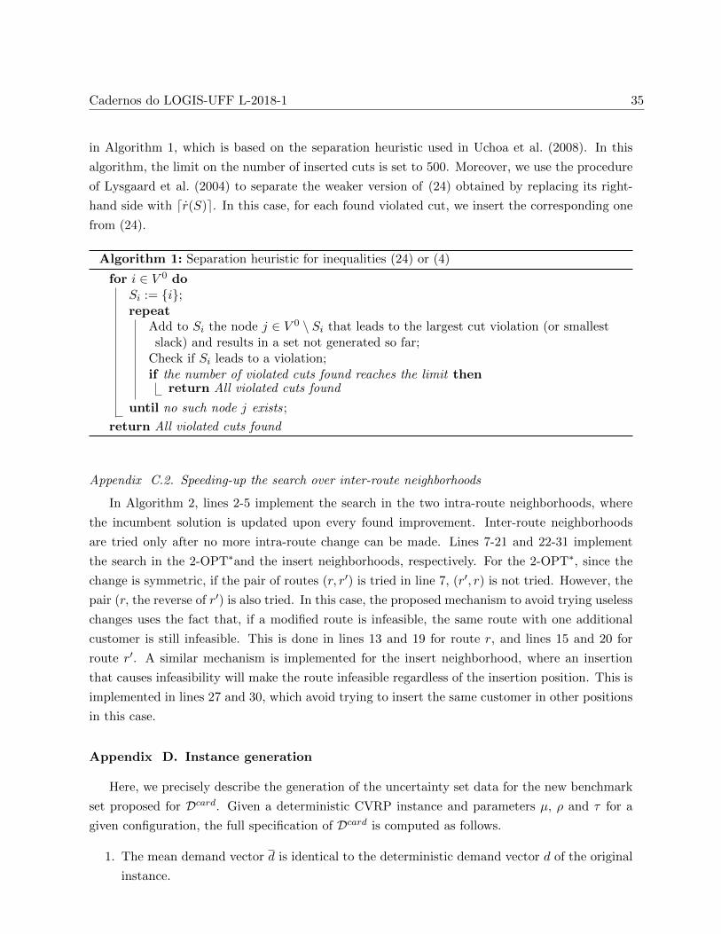
Cadernos do LOGIS-UFF L-2018-1 35
in Algorithm 1, which is based on the separation heuristic used in Uchoa et al. (2008). In this
algorithm, the limit on the number of inserted cuts is set to 500. Moreover, we use the procedure
of Lysgaard et al. (2004) to separate the weaker version of (24) obtained by replacing its right-
hand side with dr(S)e. In this case, for each found violated cut, we insert the corresponding one
from (24).
Algorithm 1: Separation heuristic for inequalities (24) or (4)
for i ∈ V 0 doSi := {i};repeat
Add to Si the node j ∈ V 0 \ Si that leads to the largest cut violation (or smallestslack) and results in a set not generated so far;
Check if Si leads to a violation;if the number of violated cuts found reaches the limit then
return All violated cuts found
until no such node j exists;
return All violated cuts found
Appendix C.2. Speeding-up the search over inter-route neighborhoods
In Algorithm 2, lines 2-5 implement the search in the two intra-route neighborhoods, where
the incumbent solution is updated upon every found improvement. Inter-route neighborhoods
are tried only after no more intra-route change can be made. Lines 7-21 and 22-31 implement
the search in the 2-OPT∗and the insert neighborhoods, respectively. For the 2-OPT∗, since the
change is symmetric, if the pair of routes (r, r′) is tried in line 7, (r′, r) is not tried. However, the
pair (r, the reverse of r′) is also tried. In this case, the proposed mechanism to avoid trying useless
changes uses the fact that, if a modified route is infeasible, the same route with one additional
customer is still infeasible. This is done in lines 13 and 19 for route r, and lines 15 and 20 for
route r′. A similar mechanism is implemented for the insert neighborhood, where an insertion
that causes infeasibility will make the route infeasible regardless of the insertion position. This is
implemented in lines 27 and 30, which avoid trying to insert the same customer in other positions
in this case.
Appendix D. Instance generation
Here, we precisely describe the generation of the uncertainty set data for the new benchmark
set proposed for Dcard. Given a deterministic CVRP instance and parameters µ, ρ and τ for a
given configuration, the full specification of Dcard is computed as follows.
1. The mean demand vector d is identical to the deterministic demand vector d of the original
instance.

Cadernos do LOGIS-UFF L-2018-1 36
Algorithm 2: Local Search (parameter: an incumbent solution INC)
1 repeat2 for each possible 2-OPT move over INC do3 if it improves INC then replace INC by the new solution
4 for each possible reinsertion move over INC do5 if it improves INC then replace INC by the new solution
6 if INC was not changed in the current iteration then7 for each pair of routes r and r′ in INC do8 for p = 0, . . . , |r| do9 q0 ← 0;
10 for q = q0, . . . , |r′| do11 try exchanging the last |r| − p customers of r with the last |r′| − q
customers of r′;12 if r fails in the approximate feasibility test then13 q0 ← q + 1; continue for;
14 if r′ fails in the approximate feasibility test then15 exit for;
16 if it improves the cost of INC then17 if INC fails in the exact feasibility test then18 if INC failed because of r then19 q0 ← q + 1; continue for;
20 else exit for;
21 else replace INC by the new solution
22 for each pair of routes r and r′ in INC do23 for p = 1, . . . , |r| do24 for q = 0, . . . , |r′| do25 try inserting the pth customer of r after q customers in r′;26 if r′ fails in the approximate feasibility test then27 exit for;
28 if it improves the cost of INC then29 if r′ fails in the exact feasibility test then30 exit for;
31 else replace INC by the new solution
32 until INC does not change in the current iteration;
2. d = µd.
3. Γ =⌊ρnm
⌋.
4. This last step is more involved since it aims to define a modified value for the vehicle
capacity C ensuring that the resulting instance is feasible and the capacity is not too loose

Cadernos do LOGIS-UFF L-2018-1 37
(otherwise using a smaller number of vehicles would be desirable in practice). For that, we
define a function BP(c) that receives a tentative capacity value c and computes an upper
approximation of the minimum number of vehicles required to make the current robust
CVRP instance feasible with c as the vehicle capacity. The algorithm used to evaluate BP is
detailed later. Then, we set C = τCmin+(1−τ)Cmax, where Cmin = min{c ∈ IN |BP(c) ≤ m}and Cmax = min{c ∈ IN |BP(c) ≤ m− 1}.
First, we remark that function BP(c) can be fulfilled by any heuristic for the robust counterpart
of the Bin Packing Problem (BPP). To see this, note that BP ignores the objective function of
the robust CVRP instance being processed and tries to pack the customer into the minimum
number of identical vehicles with capacity c. Thus, we compute BP using the well-known first-
fit decreasing heuristic for the deterministic version of BPP, where customers are ordered in a
non-increasing order by the sum of their maximum demands allowed by the uncertainty set. At
each iteration, the heuristic searches in the ordered list of customers for the first one that fits into
the current vehicle. Whenever no customers can be inserted in the current vehicle, a new vehicle
is inserted in the solution. Although this method is not guaranteed to compute the minimum
number of vehicles required, we observed that instances created with τ = 0 were not realistic
since their solution costs (now considering the CVRP objective function) usually increased by
large factors with respect to the deterministic version of the problem. Thus, we decided restrict
our attention to instances with τ ≥ 1.5. For the sake of easy reproducibility of our results, we
report the values of Cmin and Cmax for all instances of the proposed benchmark set in Subsection
Appendix F.1.
Appendix E. Detailed numerical experiments
Appendix E.1. Effect of preprocessing
Appendix E.1.1. Uncertainty set Dpart
Table E.5 shows the effect of the preprocessing technique introduced in Subsection 2.3 based in
Corollary 2 for Dpart. In this table, the last 4 columns shows the average number of vehicles (m),
the average number of subproblems after preprocessing (#sp), the percentage reduction (%red.)
obtained with respect to the initial number of subproblems, which is always equal to 2s = 16, and
the number of instances that could be solved as deterministic CVRP because only one subproblem
remained.
From Table E.5, it can be seen that the proposed preprocessing method is very effective for the
literature instances. Almost 80% of the subproblems have been removed, and 22 of 90 instances
were solved as deterministic CVRP. Moreover, the preprocessing method seems to be more effec-
tive for instance classes where the average number of vehicles is larger. We believe that this is
not a coincidence and that the way instances have been generated favors the observed reduction.
Recall that the limit on the total demand deviation for each quadrant is fixed as 75% of the sum

Cadernos do LOGIS-UFF L-2018-1 38
Table E.5: Effect of preprocessing for Dpart
In. cls #in. m #sp %red. #det.
A 26 7.1 2.7 83.4% 7B 23 7.2 3.9 75.8% 0E 11 7.3 3.6 77.3% 4F 3 5.0 5.0 68.8% 0M 3 9.7 1.3 91.7% 2P 24 7.3 4.3 73.2% 9
all 90 7.2 3.6 77.8% 22
of demand deviations. Since each quadrant has roughly 25% of the total demand to be served
and deviations are proportional to mean demand values, the limit imposed to the total demand
deviation can only be reached for a route the serves roughly 18.75% (> 1/6) of the total demand.
Thus, if the number vehicles is much larger than 6, the preprocessing step is likely to prove that
total deviation limit cannot be reached for many quadrants. This hypothesis is confirmed by the
chart of Figure E.2, where each point represents one or more instances whose coordinates are the
number of vehicles and the number of remaining subproblems after preprocessing. The decrease
on the number of subproblems as the number of vehicles increases is very clear.
0 2 4 6 8 10 12 14 160
2
4
6
8
10
12
14
m vs. Number of remaining subproblems
m
# of
sub
prob
lem
s
Figure E.2: Relation between the number of vehicles and the number of subproblems remaining after preprocessing.
Although the previous observation has been caused a specific artificial property of the bench-
mark set, we believe that similar situations may occur in real-life applications, leading to im-

Cadernos do LOGIS-UFF L-2018-1 39
pressive reductions on the number of subproblems. For testing robust optimization algorithms
however, it is now desirable that the new benchmark sets are designed to avoid the existence of
redundant constraints in the uncertainty set description. This is the case for the new benchmark
set proposed in Subsection 6.2.1.
Appendix E.1.2. Uncertainty set Dcard
Table E.6 presents a measure of the effect of preprocessing the subproblems. In this table,
the first seven rows after the headers refer to the main configuration described in the previous
subsection, containing results for each instance class separately, and then aggregated results. The
additional six rows provide aggregated results for all instance classes considering the remaining
configurations. The results in these rows should be compared with that in the seventh row. The
first two columns contain the instance class or configuration identifier (In. cls), and the number
of instances in that subset (#in.). Tables 4, E.8, and E.7 following the same format except that
results for configurations other than the main one are not presented in the last two tables. The
last four columns of Table E.6 contain the average number of distinct demand values (#dem.),
the average number of subproblems without preprocessing (#sp lit.) according to Theorem 2, and
the average number of subproblems after preprocessing(#sp new), and the percentage reduction
(%red.).
Table E.6: Effect of preprocessing for Dcard
In. cls #in. #dem. #sp lit. #sp new %red.
A 27 20.7 16.6 13.7 16.7%B 23 21.6 16.9 14.0 16.9%E 13 24.3 17.4 14.1 16.0%F 2 53.5 24.5 21.5 11.9%M 2 14.0 10.5 8.5 26.3%P 23 25.5 18.3 16.2 9.4%
all 90 22.7 17.0 14.4 14.7%
Low d 90 22.7 17.0 14.8 12.4%
High d 90 22.7 17.0 14.1 16.1%
Low Γ 90 22.7 17.8 17.7 0.8%High Γ 90 22.7 16.1 10.6 32.6%
Low C 90 22.7 17.0 14.2 16.0%High C 90 22.7 17.0 14.9 11.6%
From Table E.6, we observe that the effect of preprocessing is not so expressive but still
significant for the new benchmark instances. This was expected since the instances have been
generated in a way that Γ is never larger than the average route length. We also observe that the
effect of preprocessing increases for larger values of Γ, and that Theorem 2 provides an important
reduction on the number of subproblems with respect to the number of distinct demand values
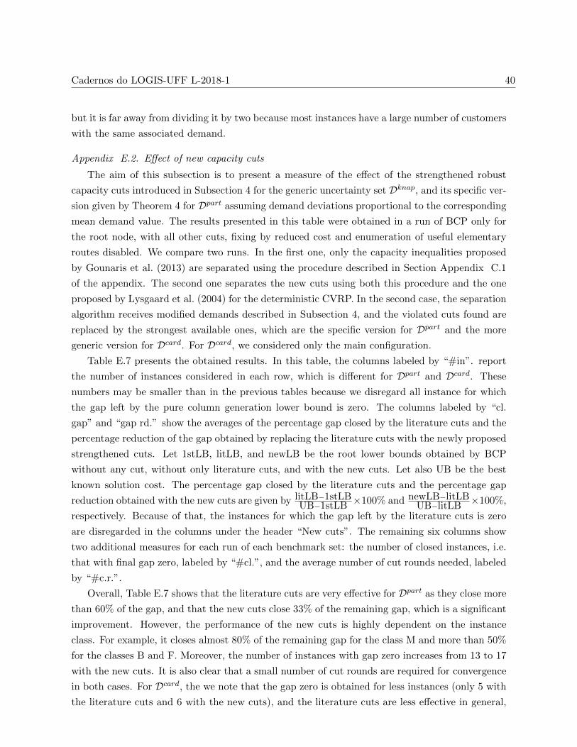
Cadernos do LOGIS-UFF L-2018-1 40
but it is far away from dividing it by two because most instances have a large number of customers
with the same associated demand.
Appendix E.2. Effect of new capacity cuts
The aim of this subsection is to present a measure of the effect of the strengthened robust
capacity cuts introduced in Subsection 4 for the generic uncertainty set Dknap, and its specific ver-
sion given by Theorem 4 for Dpart assuming demand deviations proportional to the corresponding
mean demand value. The results presented in this table were obtained in a run of BCP only for
the root node, with all other cuts, fixing by reduced cost and enumeration of useful elementary
routes disabled. We compare two runs. In the first one, only the capacity inequalities proposed
by Gounaris et al. (2013) are separated using the procedure described in Section Appendix C.1
of the appendix. The second one separates the new cuts using both this procedure and the one
proposed by Lysgaard et al. (2004) for the deterministic CVRP. In the second case, the separation
algorithm receives modified demands described in Subsection 4, and the violated cuts found are
replaced by the strongest available ones, which are the specific version for Dpart and the more
generic version for Dcard. For Dcard, we considered only the main configuration.
Table E.7 presents the obtained results. In this table, the columns labeled by “#in”. report
the number of instances considered in each row, which is different for Dpart and Dcard. These
numbers may be smaller than in the previous tables because we disregard all instance for which
the gap left by the pure column generation lower bound is zero. The columns labeled by “cl.
gap” and “gap rd.” show the averages of the percentage gap closed by the literature cuts and the
percentage reduction of the gap obtained by replacing the literature cuts with the newly proposed
strengthened cuts. Let 1stLB, litLB, and newLB be the root lower bounds obtained by BCP
without any cut, without only literature cuts, and with the new cuts. Let also UB be the best
known solution cost. The percentage gap closed by the literature cuts and the percentage gap
reduction obtained with the new cuts are given by litLB−1stLBUB−1stLB ×100% and newLB−litLB
UB−litLB×100%,
respectively. Because of that, the instances for which the gap left by the literature cuts is zero
are disregarded in the columns under the header “New cuts”. The remaining six columns show
two additional measures for each run of each benchmark set: the number of closed instances, i.e.
that with final gap zero, labeled by “#cl.”, and the average number of cut rounds needed, labeled
by “#c.r.”.
Overall, Table E.7 shows that the literature cuts are very effective for Dpart as they close more
than 60% of the gap, and that the new cuts close 33% of the remaining gap, which is a significant
improvement. However, the performance of the new cuts is highly dependent on the instance
class. For example, it closes almost 80% of the remaining gap for the class M and more than 50%
for the classes B and F. Moreover, the number of instances with gap zero increases from 13 to 17
with the new cuts. It is also clear that a small number of cut rounds are required for convergence
in both cases. For Dcard, the we note that the gap zero is obtained for less instances (only 5 with
the literature cuts and 6 with the new cuts), and the literature cuts are less effective in general,
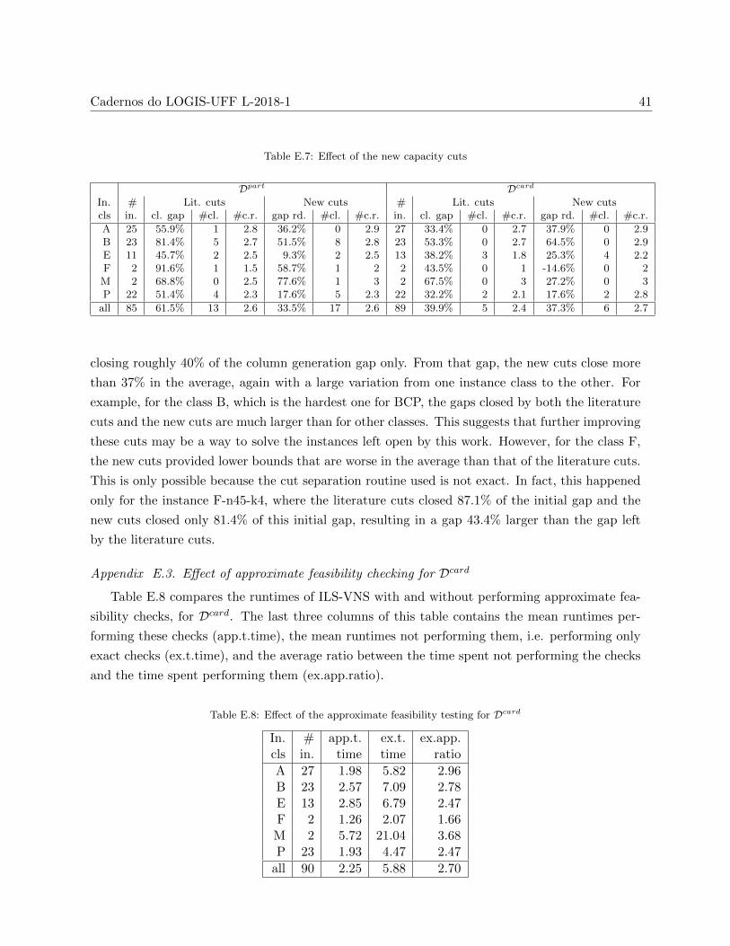
Cadernos do LOGIS-UFF L-2018-1 41
Table E.7: Effect of the new capacity cuts
Dpart Dcard
In. # Lit. cuts New cuts # Lit. cuts New cutscls in. cl. gap #cl. #c.r. gap rd. #cl. #c.r. in. cl. gap #cl. #c.r. gap rd. #cl. #c.r.
A 25 55.9% 1 2.8 36.2% 0 2.9 27 33.4% 0 2.7 37.9% 0 2.9B 23 81.4% 5 2.7 51.5% 8 2.8 23 53.3% 0 2.7 64.5% 0 2.9E 11 45.7% 2 2.5 9.3% 2 2.5 13 38.2% 3 1.8 25.3% 4 2.2F 2 91.6% 1 1.5 58.7% 1 2 2 43.5% 0 1 -14.6% 0 2M 2 68.8% 0 2.5 77.6% 1 3 2 67.5% 0 3 27.2% 0 3P 22 51.4% 4 2.3 17.6% 5 2.3 22 32.2% 2 2.1 17.6% 2 2.8
all 85 61.5% 13 2.6 33.5% 17 2.6 89 39.9% 5 2.4 37.3% 6 2.7
closing roughly 40% of the column generation gap only. From that gap, the new cuts close more
than 37% in the average, again with a large variation from one instance class to the other. For
example, for the class B, which is the hardest one for BCP, the gaps closed by both the literature
cuts and the new cuts are much larger than for other classes. This suggests that further improving
these cuts may be a way to solve the instances left open by this work. However, for the class F,
the new cuts provided lower bounds that are worse in the average than that of the literature cuts.
This is only possible because the cut separation routine used is not exact. In fact, this happened
only for the instance F-n45-k4, where the literature cuts closed 87.1% of the initial gap and the
new cuts closed only 81.4% of this initial gap, resulting in a gap 43.4% larger than the gap left
by the literature cuts.
Appendix E.3. Effect of approximate feasibility checking for Dcard
Table E.8 compares the runtimes of ILS-VNS with and without performing approximate fea-
sibility checks, for Dcard. The last three columns of this table contains the mean runtimes per-
forming these checks (app.t.time), the mean runtimes not performing them, i.e. performing only
exact checks (ex.t.time), and the average ratio between the time spent not performing the checks
and the time spent performing them (ex.app.ratio).
Table E.8: Effect of the approximate feasibility testing for Dcard
In. # app.t. ex.t. ex.app.cls in. time time ratio
A 27 1.98 5.82 2.96B 23 2.57 7.09 2.78E 13 2.85 6.79 2.47F 2 1.26 2.07 1.66M 2 5.72 21.04 3.68P 23 1.93 4.47 2.47
all 90 2.25 5.88 2.70

Cadernos do LOGIS-UFF L-2018-1 42
Appendix F. Raw data for Reproducibility
Appendix F.1. Capacity ranges for the new benchmark set
Table F.9: Minimum and maximum capacities for Dcard
Inst. Cmin Cmin Inst. Cmin Cmin Inst. Cmin Cmin
A-n32-k5 104 126 B-n38-k6 108 126 E-n76-k14 123 132
A-n33-k5 111 135 B-n39-k5 111 135 E-n101-k8 228 258
A-n33-k6 115 134 B-n41-k6 120 141 E-n101-k14 130 140
A-n34-k5 116 139 B-n43-k6 110 129 F-n45-k4 2275 3019
A-n36-k5 112 137 B-n44-k7 115 132 F-n72-k4 36382 48097
A-n37-k5 104 128 B-n45-k5 124 151 M-n101-k10 231 251
A-n37-k6 119 140 B-n45-k6 124 146 M-n121-k7 244 280
A-n38-k5 121 148 B-n50-k7 110 127 P-n19-k2 194 358
A-n39-k5 121 148 B-n50-k8 116 129 P-n20-k2 196 363
A-n39-k6 110 129 B-n51-k7 123 141 P-n21-k2 186 347
A-n44-k6 120 141 B-n52-k7 109 125 P-n22-k2 193 357
A-n45-k6 125 147 B-n56-k7 110 126 P-n22-k8 3420 3790
A-n45-k7 114 129 B-n57-k7 127 145 P-n23-k8 50 57
A-n46-k7 108 123 B-n57-k9 112 124 P-n40-k5 155 188
A-n48-k7 114 130 B-n63-k10 116 127 P-n45-k5 173 210
A-n53-k7 121 140 B-n64-k9 124 137 P-n50-k7 170 195
A-n54-k7 121 138 B-n66-k9 121 134 P-n50-k8 148 166
A-n55-k9 116 129 B-n67-k10 114 124 P-n50-k10 117 128
A-n60-k9 115 128 B-n68-k9 117 130 P-n51-k10 96 106
A-n61-k9 124 138 B-n78-k10 119 130 P-n55-k7 184 209
A-n62-k8 116 131 E-n13-k4 5820 7420 P-n55-k8 164 184
A-n63-k9 124 138 E-n22-k4 6940 9000 P-n55-k10 131 143
A-n63-k10 117 129 E-n23-k3 5330 6266 P-n55-k15 85 90
A-n64-k9 120 133 E-n30-k3 5330 7865 P-n60-k10 141 155
A-n65-k9 123 137 E-n31-k7 163 190 P-n60-k15 91 96
A-n69-k9 118 131 E-n33-k4 9260 12129 P-n65-k10 150 165
A-n80-k10 118 130 E-n51-k5 194 237 P-n70-k10 164 181
B-n31-k5 103 126 E-n76-k7 245 280 P-n76-k4 427 553
B-n34-k5 115 141 E-n76-k8 214 241 P-n76-k5 341 416
B-n35-k5 111 137 E-n76-k10 170 186 P-n101-k4 457 594
Appendix F.2. Raw ILS-VNS results for Dpart

Cadernos do LOGIS-UFF L-2018-1 43
Inst. UB avg t. min t. max t. Inst. UB avg t. min t. max t.
A-n32-k5 748 0.30 0.30 0.31 B-n66-k9 1251 2.75 0.93 6.49
A-n33-k5 642 0.28 0.24 0.31 B-n67-k10 1007 1.15 1.04 1.61
A-n33-k6 717 0.30 0.26 0.55 B-n68-k9 1205 31.25 1.84 112.23
A-n34-k5 715 0.32 0.29 0.38 B-n78-k10 1131 6.57 1.29 20.89
A-n36-k5 755 0.40 0.30 0.64 E-n22-k4 373 0.14 0.14 0.14
A-n37-k5 650 0.41 0.37 0.45 E-n23-k3 563 0.29 0.22 0.52
A-n37-k6 892 0.31 0.30 0.33 E-n30-k3 475 0.29 0.28 0.29
A-n38-k5 704 1.20 0.40 3.84 E-n33-k4 814 0.37 0.37 0.37
A-n39-k5 777 0.64 0.37 1.36 E-n51-k5 516 0.84 0.81 0.88
A-n39-k6 787 0.40 0.38 0.49 E-n76-k7 661 4.20 1.56 8.87
A-n44-k6 909 2.35 0.60 4.32 E-n76-k8 709 7.30 1.43 13.69
A-n45-k6 896 2.50 1.42 4.52 E-n76-k10 796 42.78 5.95 173.49
A-n46-k7 888 0.62 0.53 1.04 E-n76-k14 952 1.78 0.93 3.50
A-n48-k7 1033 0.63 0.53 0.96 E-n101-k8 789 8.90 2.93 21.58
A-n53-k7 974 0.71 0.59 0.93 E-n101-k14 1011 7.40 1.98 16.40
A-n54-k7 1106 2.32 0.52 7.68 F-n45-k4 718 0.85 0.64 1.18
A-n55-k9 1030 3.68 1.49 8.98 F-n72-k4 232 2.10 2.04 2.20
A-n60-k9 1280 1.66 0.86 4.14 F-n135-k7 1122 112.18 30.99 428.40
A-n61-k9 983 87.32 1.74 309.07 M-n101-k10 809 2.97 2.84 3.34
A-n62-k8 1219 4.29 1.05 10.08 M-n121-k7 994 6.83 3.11 13.04
A-n63-k9 1505 7.75 1.66 14.44 M-n151-k12 987 921.55 35.81 2416.68
A-n63-k10 1244 3.34 1.36 7.73 P-n16-k8 439 0.05 0.05 0.05
A-n64-k9 1326 2.78 0.89 5.08 P-n19-k2 195 0.12 0.12 0.12
A-n65-k9 1106 4.85 1.28 13.12 P-n20-k2 208 0.15 0.15 0.15
A-n69-k9 1109 7.13 1.71 12.66 P-n21-k2 208 0.17 0.16 0.17
A-n80-k10 1662 16.17 3.48 38.97 P-n22-k2 213 0.17 0.17 0.17
B-n31-k5 651 0.25 0.24 0.28 P-n22-k8 537 0.09 0.09 0.09
B-n34-k5 768 0.31 0.30 0.31 P-n23-k8 504 0.14 0.09 0.30
B-n35-k5 883 0.31 0.26 0.37 P-n40-k5 447 0.60 0.41 1.15
B-n38-k6 729 0.39 0.38 0.39 P-n45-k5 501 0.64 0.60 0.67
B-n39-k5 532 0.42 0.39 0.52 P-n50-k7 539 2.43 0.59 7.15
B-n41-k6 796 0.39 0.35 0.50 P-n50-k8 592 0.60 0.45 0.97
B-n43-k6 681 0.49 0.47 0.52 P-n50-k10 656 0.58 0.43 0.90
B-n44-k7 835 0.37 0.35 0.38 P-n51-k10 707 1.58 0.82 2.98
B-n45-k5 701 0.56 0.55 0.58 P-n55-k7 549 2.27 0.74 5.54
B-n45-k6 660 0.51 0.44 0.89 P-n55-k8 572 1.24 0.69 2.67

Cadernos do LOGIS-UFF L-2018-1 44
B-n50-k7 679 0.73 0.66 0.97 P-n55-k10 670 1.59 0.60 2.56
B-n50-k8 1224 5.97 0.98 15.52 P-n55-k15 889 1.04 0.48 2.17
B-n51-k7 961 2.85 0.66 7.22 P-n60-k10 712 0.82 0.65 1.95
B-n52-k7 675 0.88 0.71 1.32 P-n60-k15 931 26.82 2.50 74.61
B-n56-k7 623 0.78 0.76 0.80 P-n65-k10 765 8.40 1.33 21.81
B-n57-k7 1055 0.86 0.67 1.27 P-n70-k10 785 2.59 0.71 6.69
B-n57-k9 1540 25.60 2.42 67.59 P-n76-k4 590 3.75 2.45 6.01
B-n63-k10 1407 3.05 0.60 7.17 P-n76-k5 616 3.64 1.94 8.64
B-n64-k9 803 0.93 0.90 0.99 P-n101-k4 673 5.43 4.60 7.08
Appendix F.3. Raw BCP results for Dpart
Inst. root LB UB time Inst. root LB UB time
A-n32-k5 748.0 748 0.42 B-n66-k9 1249.2 1251 47.11
A-n33-k5 630.7 642 2.65 B-n67-k10 1006.0 1007 13.03
A-n33-k6 705.7 717 0.60 B-n68-k9 1204.1 1205 24.46
A-n34-k5 708.8 715 0.60 B-n78-k10 1130.3 1131 24.73
A-n36-k5 742.0 755 1.46 E-n22-k4 362.5 373 1.75
A-n37-k5 645.4 650 1.96 E-n23-k3 550.3 563 8.23
A-n37-k6 881.0 892 0.72 E-n30-k3 475.0 475 19.62
A-n38-k5 698.5 704 1.37 E-n33-k4 807.3 814 35.91
A-n39-k5 775.2 777 1.87 E-n51-k5 515.0 516 5.44
A-n39-k6 777.3 787 0.81 E-n76-k7 660.2 661 20.89
A-n44-k6 902.5 909 2.99 E-n76-k8 707.5 709 12.72
A-n45-k6 894.2 896 1.82 E-n76-k10 793.7 796 8.54
A-n46-k7 885.0 888 2.68 E-n76-k14 947.6 952 2.03
A-n48-k7 1026.4 1033 4.78 E-n101-k8 788.7 789 232.46
A-n53-k7 972.0 974 12.01 E-n101-k14 1011.0 1011 7.16
A-n54-k7 1105.5 1106 7.70 F-n45-k4 715.1 718 38.41
A-n55-k9 1023.8 1030 1.89 F-n72-k4 232.0 232 173.85
A-n60-k9 1276.2 1280 4.65 F-n135-k7 1111.8 1122 86700.00
A-n61-k9 978.4 983 5.28 M-n101-k10 806.3 809 3.18
A-n62-k8 1202.6 1214 15.46 M-n121-k7 993.4 994 163.50
A-n63-k9 1503.1 1505 4.79 M-n151-k12 979.1 985 6949.66
A-n63-k10 1233.0 1233 14.47 P-n16-k8 434.5 439 0.02
A-n64-k9 1321.8 1325 16.45 P-n19-k2 195.0 195 0.63
A-n65-k9 1101.8 1106 1.09 P-n20-k2 207.8 208 0.61
A-n69-k9 1105.5 1109 8.75 P-n21-k2 207.3 208 1.14
A-n80-k10 1659.1 1662 13.68 P-n22-k2 209.9 213 1.21

Cadernos do LOGIS-UFF L-2018-1 45
B-n31-k5 649.8 651 0.90 P-n22-k8 537.0 537 0.13
B-n34-k5 768.0 768 10.43 P-n23-k8 500.8 504 0.04
B-n35-k5 883.0 883 1.51 P-n40-k5 442.2 447 1.18
B-n38-k6 728.3 729 1.16 P-n45-k5 496.7 501 4.73
B-n39-k5 532.0 532 9.64 P-n50-k7 535.0 539 2.47
B-n41-k6 793.9 796 4.29 P-n50-k8 586.8 592 0.34
B-n43-k6 678.7 681 4.36 P-n50-k10 650.7 656 0.24
B-n44-k7 833.7 835 1.51 P-n51-k10 698.7 707 0.42
B-n45-k5 698.5 701 16.32 P-n55-k7 546.4 549 5.44
B-n45-k6 656.9 660 5.50 P-n55-k8 569.1 572 6.43
B-n50-k7 679.0 679 2.40 P-n55-k10 666.3 670 3.48
B-n50-k8 1222.5 1224 5.35 P-n55-k15 880.8 889 0.20
B-n51-k7 956.9 961 5.57 P-n60-k10 707.0 712 1.36
B-n52-k7 672.0 675 7.88 P-n60-k15 922.8 931 0.71
B-n56-k7 622.1 623 6.76 P-n65-k10 761.9 765 4.06
B-n57-k7 1052.9 1055 7.99 P-n70-k10 782.4 785 1.44
B-n57-k9 1539.1 1540 4.62 P-n76-k4 589.4 590 98.61
B-n63-k10 1407.0 1407 5.40 P-n76-k5 615.4 616 73.24
B-n64-k9 801.4 803 6.45 P-n101-k4 672.7 673 373.37
* Root LB value correspond to gap 1 value on Table 2.
** Only underlined UB values are not proved to be optimal
Appendix F.4. Raw ILS-VNS results for Dcard
Inst. UB avg t. min t. max t. Inst. UB avg t. min t. max t.
A-n32-k5 857 0.27 0.24 0.29 B-n64-k9 865 260.78 38.08 976.54
A-n33-k5 675 0.27 0.25 0.34 B-n66-k9 1319 4.14 1.62 10.42
A-n33-k6 758 0.42 0.25 1.09 B-n67-k10 1086 1.13 0.63 1.68
A-n34-k5 776 0.29 0.28 0.31 B-n68-k9 1298 20.30 2.50 69.54
A-n36-k5 823 0.42 0.30 0.79 B-n78-k10 1261 1305.63 157.17 3065.41
A-n37-k5 706 0.38 0.36 0.40 E-n13-k4 277 0.02 0.02 0.02
A-n37-k6 948 2.76 0.69 9.44 E-n22-k4 373 0.13 0.12 0.13
A-n38-k5 714 0.37 0.36 0.40 E-n23-k3 570 0.23 0.23 0.23
A-n39-k5 818 0.88 0.40 1.74 E-n30-k3 495 0.33 0.32 0.34
A-n39-k6 850 0.63 0.35 0.92 E-n31-k7 379 0.21 0.17 0.23
A-n44-k6 930 0.55 0.45 0.93 E-n33-k4 836 0.37 0.35 0.42
A-n45-k6 918 1.44 0.46 6.10 E-n51-k5 519 1.32 0.69 2.92
A-n45-k7 1163 8.31 0.55 29.40 E-n76-k7 699 5.07 1.85 11.90

Cadernos do LOGIS-UFF L-2018-1 46
A-n46-k7 988 0.52 0.39 0.84 E-n76-k8 736 11.34 1.93 29.46
A-n48-k7 1129 2.91 0.52 9.89 E-n76-k10 830 385.70 66.56 895.89
A-n53-k7 1019 1.91 0.99 4.47 E-n76-k14 1022 171.57 61.57 421.72
A-n54-k7 1169 3.41 0.77 8.77 E-n101-k8 826 25.06 3.41 81.78
A-n55-k9 1107 2.72 1.09 7.46 E-n101-k14 1121 419.22 6.58 1557.43
A-n60-k9 1408 6.62 2.45 12.19 F-n45-k4 736 0.74 0.72 0.78
A-n61-k9 1022 2.55 0.89 4.76 F-n72-k4 236 2.13 2.00 2.26
A-n62-k8 1339 9.73 3.11 18.01 M-n101-k10 918 3.87 1.80 7.70
A-n63-k9 1620 7.85 1.44 23.39 M-n121-k7 1030 8.47 4.58 14.39
A-n63-k10 1348 9.87 1.77 26.70 P-n19-k2 195 0.14 0.14 0.15
A-n64-k9 1417 26.56 4.24 65.36 P-n20-k2 208 0.18 0.18 0.18
A-n65-k9 1184 3.69 1.01 12.21 P-n21-k2 208 0.19 0.19 0.19
A-n69-k9 1177 16.96 4.21 28.54 P-n22-k2 213 0.20 0.20 0.20
A-n80-k10 1803 33.70 6.34 116.94 P-n22-k8 601 0.19 0.12 0.29
B-n31-k5 694 0.23 0.19 0.47 P-n23-k8 527 0.29 0.17 0.47
B-n34-k5 789 0.29 0.27 0.33 P-n40-k5 468 0.47 0.44 0.72
B-n35-k5 986 0.23 0.22 0.26 P-n45-k5 512 2.17 0.51 5.97
B-n38-k6 823 0.32 0.27 0.49 P-n50-k7 563 0.92 0.50 1.48
B-n39-k5 561 0.34 0.30 0.52 P-n50-k8 614 1.32 0.42 2.82
B-n41-k6 838 2.96 0.30 6.36 P-n50-k10 695 3.06 0.98 8.78
B-n43-k6 779 1.69 0.43 2.88 P-n51-k10 736 1.96 0.44 6.52
B-n44-k7 943 0.93 0.46 2.47 P-n55-k7 583 1.98 0.60 3.42
B-n45-k5 739 0.61 0.53 0.74 P-n55-k8 624 2.92 0.80 9.46
B-n45-k6 668 0.38 0.37 0.40 P-n55-k10 718 14.52 1.13 49.25
B-n50-k7 758 1.48 0.44 3.28 P-n55-k15 945 1.91 0.99 3.56
B-n50-k8 1330 24.06 8.89 73.10 P-n60-k10 755 7.40 1.44 19.94
B-n51-k7 1027 2.26 0.54 5.66 P-n60-k15 1020 117.25 37.21 310.22
B-n52-k7 775 0.58 0.45 0.84 P-n65-k10 809 8.17 1.78 18.45
B-n56-k7 740 1.20 0.96 1.75 P-n70-k10 824 37.48 2.81 88.71
B-n57-k7 1132 2.02 0.76 4.79 P-n76-k4 590 7.49 2.33 20.40
B-n57-k9 1656 21.47 4.64 52.27 P-n76-k5 621 4.24 1.77 11.39
B-n63-k10 1588 19.13 2.17 56.77 P-n101-k4 681 6.84 4.50 15.75
Appendix F.5. Raw BCP results for Dcard
Inst. root LB UB time Inst. root LB UB time
A-n32-k5 857.0 857 3.79 B-n64-k9 852.0 866 7200.00
A-n33-k5 675.0 675 6.55 B-n66-k9 1319.0 1319 97.71
A-n33-k6 758.0 758 1.22 B-n67-k10 1086.0 1086 54.20

Cadernos do LOGIS-UFF L-2018-1 47
A-n34-k5 776.0 776 2.26 B-n68-k9 1298.0 1298 63.23
A-n36-k5 823.0 823 7.79 B-n78-k10 1261.0 1261 216.35
A-n37-k5 706.0 706 3.81 E-n13-k4 277.0 277 0.17
A-n37-k6 948.0 948 9.26 E-n22-k4 373.0 373 3.39
A-n38-k5 714.0 714 4.14 E-n23-k3 570.0 570 9.98
A-n39-k5 818.0 818 36.82 E-n30-k3 495.0 495 14.10
A-n39-k6 850.0 850 6.63 E-n31-k7 378.3 379 0.76
A-n44-k6 930.0 930 3.51 E-n33-k4 836.0 836 38.69
A-n45-k6 918.0 918 10.86 E-n51-k5 519.0 519 15.18
A-n45-k7 1163.0 1163 4.85 E-n76-k7 697.0 697 148.17
A-n46-k7 988.0 988 13.18 E-n76-k8 736.0 736 95.75
A-n48-k7 1129.0 1129 47.08 E-n76-k10 830.0 830 200.64
A-n53-k7 1019.0 1019 29.49 E-n76-k14 1020.0 1020 32.34
A-n54-k7 1169.0 1169 53.05 E-n101-k8 826.0 826 909.78
A-n55-k9 1107.0 1107 21.92 E-n101-k14 1107.0 1109 1977.15
A-n60-k9 1404.1 1408 176.50 F-n45-k4 736.0 736 85.10
A-n61-k9 1022.0 1022 34.40 F-n72-k4 236.0 236 583.44
A-n62-k8 1339.0 1339 106.29 M-n101-k10 918.0 918 25.98
A-n63-k9 1612.1 1618 334.82 M-n121-k7 1030.0 1030 450.81
A-n63-k10 1348.0 1348 56.41 P-n19-k2 195.0 195 0.28
A-n64-k9 1413.7 1414 35.36 P-n20-k2 208.0 208 0.52
A-n65-k9 1184.0 1184 91.31 P-n21-k2 208.0 208 0.71
A-n69-k9 1177.0 1177 35.08 P-n22-k2 213.0 213 1.35
A-n80-k10 1795.0 1795 248.47 P-n22-k8 601.0 601 0.75
B-n31-k5 694.0 694 1.36 P-n23-k8 527.0 527 0.24
B-n34-k5 789.0 789 6.44 P-n40-k5 468.0 468 9.59
B-n35-k5 986.0 986 5.37 P-n45-k5 512.0 512 16.64
B-n38-k6 823.0 823 15.59 P-n50-k7 563.0 563 8.01
B-n39-k5 561.0 561 26.39 P-n50-k8 614.0 614 45.16
B-n41-k6 838.0 838 1876.79 P-n50-k10 695.0 695 5.49
B-n43-k6 779.0 779 25.14 P-n51-k10 736.0 736 8.61
B-n44-k7 943.0 943 25.11 P-n55-k7 583.0 583 22.13
B-n45-k5 739.0 739 46.24 P-n55-k8 624.0 624 14.93
B-n45-k6 668.0 668 19.24 P-n55-k10 718.0 718 11.86
B-n50-k7 758.0 758 6.31 P-n55-k15 945.0 945 4.70
B-n50-k8 1330.0 1330 19.70 P-n60-k10 755.0 755 29.65
B-n51-k7 1010.1 1027 7200.00 P-n60-k15 1020.0 1020 20.87
B-n52-k7 775.0 775 22.00 P-n65-k10 809.0 809 66.89

Cadernos do LOGIS-UFF L-2018-1 48
B-n56-k7 740.0 740 23.78 P-n70-k10 824.0 824 63.11
B-n57-k7 1112.8 1133 7200.00 P-n76-k4 590.0 590 267.42
B-n57-k9 1656.0 1656 77.70 P-n76-k5 621.0 621 284.10
B-n63-k10 1578.9 1587 843.21 P-n101-k4 681.0 681 2096.77
* Root LB value correspond to gap 1 value on Table 4.
** Only underlined UB values are not proved to be optimal