branch-and-lift algorithm for global optimal control
TRANSCRIPT

Branch-and-Lift Algorithm for Deterministic Global
Optimization in Nonlinear Optimal Control
Boris HOUSKA and Benoıt CHACHUAT
Centre for Process Systems Engineering (CPSE), Departmentof Chemical Engineering, Imperial College London,
South Kensington Campus, London SW7 2AZ, United Kingdom.
AbstractThis paper presents a branch-and-lift algorithm for solving optimal control problems with smooth nonlinear dy-
namics and potentially nonconvex objective and constraintfunctionals to guaranteed global optimality. This algo-
rithm features a direct sequential method and builds upon a generic, spatial branch-and-bound algorithm. A new
operation, called lifting, is introduced which refines the control parameterization via a Gram-Schmidt orthogo-
nalization process, while simultaneously eliminating control subregions that are either infeasible or that provably
cannot contain any global optima. Conditions are given under which the image of the control parameterization er-
ror in the state space contracts exponentially as the parameterization order is increased, thereby making the lifting
operation efficient. A computational technique based on ellipsoidal calculus is also developed that satisfies these
conditions. The practical applicability of branch-and-lift is illustrated in a numerical example.
Key Words:Optimal Control· Dynamic Optimization· Dynamic Systems· Deterministic Global Op-
timization· Spatial Branch-and-Bound
1 Introduction
Finding globally optimal solutions to nonlinear optimal control problems is a practically relevant, yet challenging
task. Although nonlinear optimal control methods and toolsbased on local optimization are satisfactory for
many practical purposes, they can get trapped into local optima, possibly suboptimal by a large margin. For
example in controlling a car or a robot in the presence of obstacles, a local solver will typically fail to determine
whether passing a given obstacle on the right or left is optimal. Similar situations can occur in the field of control
of (bio)chemical processes, as these processes can presentcomplex and highly nonlinear behavior leading for
instance to steady-state multiplicity. For such problems,it is often unclear how to initialize a local solver in order
to find a control input leading to the best possible performance. Moreover, there are important classes of problems
for which obtaining a certificate of global optimality is paramount. In the field of robust and scenario-integrated
optimization for instance, the lower-level optimization problems have to be solved to global optimality, as the
upper level problem may be infeasible otherwise; see, e.g.,[46].
Local optimization theory for optimal control problems is well developed and there is a wide variety of local
optimization algorithms for such problems [9, 11, 67]. As far as global optimization is concerned, only a few
numerical approaches exist, however. The focus of this paper is on deterministic global optimization methods,
and therefore we do not elaborate further on stochastic global optimal control algorithms, referring the reader
to [5, 20, 43] for an overview. Concerning deterministic global optimalcontrol algorithms, we distinguish two
classes of algorithms next, namely indirect and direct methods.
1

Indirect optimal control methods have in common that they first analyze an optimal control problem in terms
of its optimality conditions, prior to applying a numericaldiscretization. Two of the most important classes of
indirect methods are:
1. TheHamilton-Jacobi-Bellman (HJB) equationapproach, which leads to a global optimal control algorithm
known under the name dynamic programming. This technique isbased on Bellman’s optimality princi-
ple, named after the work by Bellman in the late 1950’s [6]. In practice, dynamic programming involves
back-propagating the so-called optimal value function in the state space, which limits application to opti-
mal control problems having no more than a few state variables. Nevertheless, the dynamic programming
algorithm is advantageous in that it can deal with time-varying controls directly and, most importantly, it
can determine globally optimal solutions. For an overview of state-of-the-art global optimal control based
on dynamic programming we refer the reader to [12, 28, 42]. Note also that some optimal control problems,
for instance problems with coupled boundary conditions, cannot be addressed easily within this approach.
2. ThePontryagin Maximum Principle (PMP), which leads to a boundary value problem that is amenable to
numerical solution [9, 17, 70]. This approach relies on variational analysis in order to derive first-order
necessary optimality conditions for the infinite-dimensional optimal control problem [53]. However, the
PMP only provides local optimality conditions and, to the authors’ best knowledge, no global optimal
control algorithm has been developed based on this technique to date. Although it should be possible,
at least in principle, to use the PMP to single out a set of candidate optimal controls, perhaps the major
difficulty with this approach would be of combinatorial nature since the sequence and types of arcs in an
optimal solution are not knowna priori.
Direct optimal control methods approximate the optimal control problem by a finite-dimensional nonlinear
programming (NLP) problem, which is then solved using standard numerical optimization algorithms. Three
main variants of this approach are single shooting, multiple shooting, and orthogonal collocation.
1. The idea behind thesingle shootingapproach, also known as thedirect sequentialmethod, is to parameterize
the control trajectories. The response of the dynamic systems is regarded as a function of the control
parameterization coefficients, which are the decision variables in a finite-dimensional NLP problem. The
evaluation of the objective and constraint functions in thediscretized NLP is via the numerical integration
of the differential equations. This approach was originally introduced in a local optimization context [16,
60, 67], but it has more recently been extended to global optimization, see for example [19, 21, 22, 41, 51,
57, 65]. Note that all of these approaches have in common that they rely on branch-and-bound search [30]
to solve the resulting NLP problem to guaranteed global optimality. Their practical applicability is currently
limited to optimal control problems with a small number of decision variables only, up to about 10 variables.
This is attributed to the fact that a fine control parameterization leads to an NLP problem with a large number
of degrees of freedom, and also that state-of-the art enclosure methods for nonlinear parametric differential
equations can result in rather conservative bounds or convex relaxations due to the wrapping effect. We also
note that such enclosure methods can scale poorly with the number of state variables as well, especially if
no particular structure can be exploited in the equations.
2. Themultiple shootingapproach differs from single shooting in that the time horizon is first divided into a
number of subintervals [13]. The state variables at the initial time of each subinterval become additional
decision variables in the NLP problem, state continuity at the transition times is enforced by imposing
extra constraints, and the rest of the approach remains analogous to single shooting. The multiple shooting
2

approach is available in state-of-the-art optimal controlsoftware based on local optimization solvers [31,
39], where the block structure of the NLP problem is exploited within the underlying linear algebra routines
for efficiency. This approach has not been used in a global optimization context to date, presumably due to
the fact that larger NLP problems are usually more difficult to solve using branch-and-bound search.
3. In theorthogonal collocationapproach both the control and the state trajectories are parameterized and the
residuals of the differential equations are enforced as constraints at specified collocation times [50, 68].
In the context of local optimization, this approach is frequently used in combination with large-scale NLP
solvers that exploit the block structure of the discretizedoptimization problem efficiently [11]. Concerning
global optimization, the collocation approach presents the advantage that all of the objective and constraint
functions become factorable, so that in principle standardglobal optimization solvers such asBARON
[56, 66] can be applied directly. The attendant drawback of this approach, however, is the large number of
variables and constraints, which often leads to prohibitive computational times as discussed in [24].
Summarizing the previous considerations, existing globaloptimal control algorithms based on dynamic program-
ming have run-times that scale exponentially with the number of differential states. Global optimization algorithms
based on direct methods, on the other hand, present worst-case run-times that scale exponentially with the number
of optimization variables in the discretized NLP problem approximating the solution of the original optimal con-
trol problem. Moreover,a priori parameterization of the control functions in direct methods does not allow control
over the accuracy of a given parameterization, and therefore this approach is not suitable for rigorous search of
globally optimal solutions in optimal control problems.
This paper develops a new algorithm, namedbranch-and-lift, in order to mitigate these limitations. This algo-
rithm features a direct sequential approach and involves refining the control parameterization during the search
as a means to control the error introduced by the control parameterization. Similar to the work by Galperin
and Zheng [26], the parameterization refinement process is based on Gram-Schmidt orthogonalization. We ex-
tend Galperin and Zheng’s idea in two ways here: (i) the spatial branch-and-bound algorithm is equipped with a
new lifting step that enables systematic branching in an infinite-dimensional space, namely the space of bounded
Lebesgue-integrable control functions; and, (ii) conditions are given under which the image of the control pa-
rameterization error in the state space contracts exponentially as the parameterization order is increased, thereby
making the lifting operation efficient (see Theorem1). Put together, these contributions lead to a global opti-
mization algorithm for optimal control problems that is rigorous in the sense that it brackets the actual solution to
the optimal control problem. Moreover, finite convergence to anǫ-suboptimal solution is established for certain
classes of optimal control problems (see Theorem2 and Corollaries1 and2). With regard to the contribution (ii), it
is worth mentioning the convex relaxation technique for optimal control problems developed by [61], which could
also be used to compute valid lower bounds in the proposed branch-and-lift algorithm. Concerning the contribu-
tion (i), mention should be made of the so-called ‘Russian Doll Algorithm’ (RDA) proposed by [69] as a variant of
branch-and-bound for constraint satisfaction problems. In RDA, the optimization is performed sequentially over
subsets of increasing dimensions, thus presenting some similarities with the lifting operation in the branch-and-lift
algorithm.
The remainder of this paper is organized as follows. The optimal control formulation and blanket assumptions are
given in Sect.2. In Sect.3 we review existing control parameterization strategies aswell as branch-and-bound
search applied to direct optimal control methods. In Sect.4 we define the image of the control discretization error
in state space and discuss its properties. The first main contribution of the paper is presented in Theorem1, where
exponential convergence of the image of the control discretization error is established under mild conditions.
The second principal contribution follows in Sect.5, where the new lifting operation is introduced as a means to
3

refine the control parameterization during the search and where the branch-and-lift algorithm is described and its
convergence properties are analyzed. We illustrate the practical applicability of branch-and-lift in Sect.6 through
a detailed numerical case study, before concluding the paper in Sect.7.
2 Problem Statement
We consider nonlinear optimal control problems (OCPs) of the form
V := minx,u
Ψ(x(T )) s.t.
x(t) = f(x(t)) +G(x(t))u(t)
x(0) = x0
x(t) ∈ Fx(t)
u(t) ∈ Fu(t) ,
(1)
where the constraints have to be satisfied for allt in a given time horizon[0, T ]. Here,x : [0, T ] → Rnx denotes
the state vector, with given initial value vectorx0 ∈ Rnx , andu : [0, T ]→ Rnu is a Lebesgue-integrable control
input vector. Moreover, we introduce the following technical blanket assumptions:
A1: The Mayer termΨ : Rnx → R is a Lipschitz-continuous function.
A2: The functionsf : Rnx → Rnx andG : Rnx → Rnx×nu are smooth and globally Lipschitz-continuous.
A3: The constraint setsFx(t) ⊆ Rnx are closed inRnx for all t ∈ [0, T ].
A4: The constraint setsFu(t) ⊂ Rnu are compact inRnu for all t ∈ [0, T ].
The problem formulation (1) and the blanket assumptions A1-A4 are introduced in an objective to keep the nota-
tion and analysis in the paper as simple as possible, although the methods presented in the following sections can
be generalized to a wider class of problems. This includes OCPs having additional finite dimensional parameters
or the initial value as additional optimization variables;OCPs with periodic or more generally coupled boundary
conditions and with mixed control-state path constraints;OCPs with non-autonomous right-hand side functionsf
andG; as well as OCPs having an additional Lagrange term in the objective function.
Assumption A2 thatf andG are globally Lipschitz continuous is introduced so as to guarantee existence and
uniqueness of the differential equation solutions, thereby ruling out the possibility of a finite escape time. A
discussion about how to extend the developed algorithms to the case thatf andG are locally, yet not globally,
Lipschitz continuous is provided later on. Moreover, the setsFx(t) in Assumption A3 are assumed to be closed,
but not necessarily compact. In particular, this includes the case that no state constraints are present in the problem.
The problem formulation (1) also assumes that the control functionu enters the right-hand side function affinely.
While the reasons for making this assumption will be explained later, it is worth mentioning at this point that many
controlled physical systems are naturally affine in their control variables. In mechanical systems, for instance,
typically control inputs are forces or torques which enter affinely in the dynamic system via Newton’s law, even
in the presence of nonlinear centrifugal, friction, or Coriolis effects; in controlled chemical reactors too, feed
rates normally enter the conservation equations affinely, despite the possible presence of nonlinear reaction rates;
and similarly in electrical circuits, controlled potential differences enter charge conservation equations affinely,
regardless of the fact that resistances, diodes or other electric devices with nonlinear characteristics may be present.
Moreover, in the case that we encounter a nonlinear differential equation inu, a reformulation as (1) can be made
under the additional assumption thatu is Lipschitz continuous. This way, the original controlu can be regarded
as an extra state satisfying an auxiliary ODE of the formu(t) = v(t), wherev is the new control variable subject
to−L ≤ v(t) ≤ L, with L the Lipschitz constant ofu on [0, T ].
4

2.1 Notation
Besides standard mathematical notation, we writeR+ := {x ∈ R | x ≥ 0} andR++ := {x ∈ R | x > 0}.
Moreover, we denote bySn+ ⊆ Rn×n the set of all symmetric positive-semidefiniten × n-matrices, and by
Sn++ ⊆ Sn+ the set of symmetric positive-definite matrices. We use
E(c,Q) :={
c+Q12 v∣
∣
∣ v ∈ Rn , vTv ≤ 1}
⊆ Rn
to denote an ellipsoid with centerc ∈ Rn and positive-semidefinite matrixQ ∈ Sn+, and we denote by
I(c, r) := {v ∈ Rn | −r ≤ v − c ≤ r} ⊆ Rn
an interval with midpointc ∈ Rn and width2r, with r ∈ Rn+. Moreover, the functionmid (I(c, r)) = c returns
the midpoint of an interval.
Given a compact setX ⊆ Rn and a norm‖ · ‖ : Rn → R, we use the notation
diam (X) := maxx,y∈X
‖x− y‖
for the associated diameter of the setX . Moreover, the power set ofX , namely the set of subsets ofX including
the empty set, is denoted byP(X). The Minkowski sum and the Minkowski difference of two setsX andY are
defined, respectively, as
X ⊕ Y := { x+ y | x ∈ X , y ∈ Y } and X ⊖ Y := { x | {x} ⊕ Y ⊆ X } .
Throughout the paper, all (time) trajectories are understood to be Lebesgue integrable and all integrals are under-
stood in the sense of Lebesgue; we denote byL2[0, T ]n the set ofn-dimensional,L2-integrable functions on the
interval [0, T ]. By an abuse of language, we say that a statement holds for allt ∈ [0, T ] at times, but mean that
this statement holds for allt ∈ [0, T ] \ L0, whereL0 can be any subset of[0, T ] with Lebesgue-zero measure.
By convention, the optimal value of a minimization (resp. maximization) problem is taken as+∞ (resp.−∞) if
the constraints are infeasible; that is,V =∞ whenever Problem (1) is infeasible.
3 Background
This section reviews and formalizes concepts for the directsequential approach of optimal control as well as its
application within spatial branch-and-bound. The formalism introduced in this section is used throughout the
paper.
3.1 Control Parameterization
It has already been mentioned that direct methods parameterize the control trajectories, so that an optimal con-
trol problem is approximated by a finite-dimensional NLP. Toformalize the concept of control parameteriza-
tion, we start by introducing a sequence ofL2-integrable basis functionsΦ0,Φ1, . . .ΦM : [0, T ] → R, which
are orthogonal with respect to a given bounded weighting function µ : [0, T ] → R++ and scaling factors
σ0, σ1, . . . σM ∈ R++:
∀i, j ∈ {0, . . . ,M}1
σi
∫ T
0
Φi(τ)Φj(τ)µ(τ) dτ = δi,j :=
{
0 if i 6= j,
1 otherwise.
5

The Gram-Schmidt coefficientsa0, . . . , aM ∈ Rnu for anL2-integrable functionω : [0, T ]→ Rn on the interval
[0, T ] are defined as
∀i ∈ {0, . . . ,M} ai :=1
σi
∫ T
0
ω(τ)Φi(τ)µ(τ) dτ.
When it is clear from the context on which time interval the integral is evaluated, we make use of the following
short-hand notation for the component-wise scalar product:
∀ω ∈ L2[0, T ]n , ∀ζ ∈ L2[0, T ] 〈ω, ζ〉µ :=
∫ T
0
ω(τ)ζ(τ)µ(τ) dτ .
The firstM + 1 Gram-Schmidt coefficients of a control input are ordered into the vectora of dimensionna =
(M + 1)nu < ∞ as follows:
a :=(
aT0 , . . . , aTM)T
∈ Rna with ai = 〈u,Φi〉µ . (2)
Fundamental properties of orthogonal decompositions ofL2 integrable functions are recalled in the next proposi-
tion.
Proposition 1. Letu beL2-integrable on[0, T ] and let the vectora be defined as in(2). The following statements
hold:
1. The firstM +1 Gram-Schmidt coefficients of the control parameterizationdefect(
u−∑M
i=0 aiΦi
)
are all
equal to zero:
∀i ∈ {0, . . . ,M}
⟨
u−
M∑
j=0
ajΦj , Φi
⟩
µ
= 0 .
2. Bessel’s inequality for the coefficient sequencea0, a1, . . . , aM is satisfied:
∀j ∈ {1, . . . , nu}M∑
i=0
σi(ai)2j ≤ 〈uj , uj〉µ .
Example 1. A piecewise constant control parameterization overM + 1 stages of equal durationh := TM+1 can
be obtained by using the orthogonal functions
∀i ∈ {0, . . . ,M} Φi(t) =
{
1 if ih ≤ t ≤ (i+ 1)h
0 otherwise ,
together with with the weighting functionµ(t) = 1 and scaling factorsσi = h for all indicesi ∈ {0, . . . ,M}. ⋄
The direct single-shooting algorithm presented in the following section relies on control parameterization using
orthogonal basis functions.
3.2 Direct Single Shooting Revisited
The main idea behind single-shooting algorithms is to approximate the infinite-dimensional optimal control prob-
lem (1) with a finite dimensional NLP problem in the variablesa, as defined previously in Sect.3.1. In order to
6

formalize this concept, we denote byy(t, a) the solution of the parametric differential equation
∀t ∈ [0, T ] y(t, a) = f(y(t, a)) +G(y(t, a))
(
M∑
i=0
aiΦi(t)
)
(3)
with y(0, a) = x0 .
Notice thaty(t, a) is well-defined, if the blanket assumption A2 is satisfied. For any closed domainA ⊆ Rna , we
introduce the finite-dimensional optimization problem
VM (A) := mina∈A
Ψ(y(T, a)) s.t.
y(t, a) ∈ Fx(t)∑M
i=0 aiΦi(t) ∈ Fu(t) ,(4)
where the constraints have to be satisfied for allt ∈ [0, T ]. The single-shooting approach computes the optimal
valueVM (Rna), and this value yields an upper bound on the actual optimal valueV of optimal control problem (1):
VM (Rna) ≥ V . (5)
Moreover, because Problem (4) yields an optimization problem with a finite number of decision variables, it can
in principle be tackled with any existing local or global optimization algorithm. The focus in the next subsection
is on spatial branch-and-bound.
3.3 Spatial Branch-and-Bound for Direct Single Shooting
Spatial branch-and-bound [25, 49] for direct single shooting starts with an initial partition A = {A0}, where
A0 ⊆ Rna is a compact set satisfying
A0 ⊇ D∗ :=
{
a ∈ Rna
∣
∣
∣
∣
∣
∀t ∈ [0, T ]M∑
i=0
aiΦi(t) ∈ Fu(t)
}
. (6)
Notice that the setD∗ is compact if Assumption A4 is satisfied. Consequently, the branch-and-bound method can
always be initialized by choosing a sufficiently large intervalA0 containing the setD∗. Branching and fathoming,
the two main operations in spatial branch-and-bound, are reviewed next.
Branching Operation This operation updates a non-empty partitionA by subdividing any setA ∈ A into two∗
compact subsetsAl andAr, with Al ∪ Ar = A, and defining
A ← A+ := (A \ {A }) ∪ {Al ,Ar} .
Many heuristics can be applied for deciding which set inA should be subdivided in priority and how to make the
subdivision—see for instance [1, 7]. From a theoretical standpoint, the basic requirement forconvergence is that
the subdivision process is exhaustive, which requires that
diam (A) := maxA∈A
diam (A) → 0 . (7)
∗In a more general implementation of the branching operation, the setA can be subdivided into more than two subsets. This is useful,forinstance, when running the algorithm on a multiprocessor computer, thereby enabling multiple branches to be analyzed in parallel.
7

Fathoming Operation Suppose that upper and lower boundsUM (A) andLM (A) can be computed such that
LM (A) ≤ VM (A) ≤ UM (A) ,
for any compact setA in a non-empty partitionA. If any elementA ∈ A is such that
LM (A) = ∞ or ∃A′ ∈ A LM (A) > UM (A′) ,
then it can be safely discarded fromA by applying the fathoming operation:
A ← A+ := A \ {A } .
It can be established [30] that the spatial branch-and-bound algorithm for direct single shooting will converge to
the optimal valueVM (Rna), if the following two conditions are satisfied:
1. The subdivision process is exhaustive; that is, condition (7) is satisfied.
2. For every sequenceA1,A2, . . . ⊆ Rna of compact sets withlimi→∞ diam (Ai) = 0 and
lim supi→∞ LM (Ai) < ∞ the upper and lower bounds are converging; that is, the following condition
is satisfied:
limi→∞
UM (Ai)− LM (Ai) = 0 .
It is common practice to interrupt the spatial branch-and-bound algorithm as soon as the condition
minA∈A
{UM (A)} − minA∈A
{LM (A)} ≤ ε
is met for a desired finite accuracyε > 0, hence providing so-calledε-suboptimal solutions of Problem (4) after a
finite number of branch-and-bound iterations.
3.4 Lower and Upper Bounding Strategy for Direct Single Shooting
For a given compact setA, a lower boundLM (A) and an upper boundUM (A) on the optimal valueVM (A) can
be found using Algorithm 1. Notice that these bounds can be either finite or infinite.
A number of comments are in order regarding the steps in Algorithm 1.
• In Step1, computing the setD∗ as defined in (6) involves checking a semi-infinite inequality of the form
∀t ∈ [0, T ]
M∑
i=0
aiΦi(t) ∈ Fu(t) .
Although a hard problem in general, this semi-infinite inequality can be rewritten equivalently as a linear
matrix inequality (LMI) in the coefficientsa0, . . . , aM when theΦi’s are polynomial functions and the sets
Fu(t) are intervals, e.g., by using the sum-of-squares approach [38]. This way, the feasibility check can be
performed using efficient convex optimization techniques.
• A major difficulty in Step2 is the computation of the outer-approximation functionY (·,A) on the solution
set of the parametric ODE (3) on [0, T ]. The quality of this enclosure function contributes significantly to the
performance of the branch-and-bound algorithm, as poor state bounds generally lead to an explosion in the
8

Algorithm 1: Computing lower and upper bounds LM (A) and UM (A) for VM (A)
Input: Compact setA ∈ A.
Algorithm:
1. If A ∩ D∗ = ∅, returnLM (A) = UM (A) = ∞.
2. Compute compact inner and outer approximationsY (t,A), Y (t,A) ⊆ Rnx such that
∀t ∈ [0, T ] Y (t,A) ⊆⋃
a∈A
{y(t, a)} ⊆ Y (t,A) .
3. If there existst ∈ [0, T ] with Y (t,A) ∩ Fx(t) = ∅, returnLM (A) = ∞ andUM (A) = ∞; otherwise, solve thelower-bounding problem
LM (A) = miny
Ψ(y) s.t. y ∈ Y (T,A) .
4. If Y (t,A) ⊆ Fx(t) for all t ∈ [0, T ], solve the upper-bounding problem
UM (A) = miny
Ψ(y) s.t. y ∈ Y (T,A) ;
otherwise, returnUM (A) = ∞.
Output: Lower and upper boundsLM (A) ≤ VM (A) ≤ UM (A).
size of the partitionA. Major differences between the existing techniques for global optimal control based
on direct single shooting are in the way these bounds are generated. In [51], the state bounds are obtained
based on the theory of differential inequalities [71]. In contrast, pointwise-in-time, convex and concave
bounds on the parametric ODE solutions are considered in [59, 62–64] based on the McCormick relaxation
technique [44]. In another approach, interval enclosures are derived from a Taylor model of the parametric
ODE solutions [8, 41, 48]. This latter approach was later extended to enable convex and concave bounds
in [58] using so-called McCormick-Taylor models [14]. The computation of guaranteed state bounds has
also been considered in different contexts, including reachability analysis and robust control [33, 36, 37].
In principle, such ellipsoidal bounds could be used in global optimal control methods too, although there
seems to be no literature on this yet. We also note that, in order for the branch-and-bound algorithm to
converge, the enclosuresY (t,A) must be convergent, i.e.,
limi→∞
diam(
Y (t,Ai))
= 0
for all t ∈ [0, T ] and for all sequencesA1,A2 . . . ⊆ Rna of compact sets, such thatlimi→∞ diam(Ai) = 0
andlim supi→∞ LM (Ai) <∞.
• The computation of inner-approximation functionsY (·,A) on the solution set of the parametric ODE (3)
on [0, T ] presents less difficulty thanY (·,A), since such a function can always be obtained, e.g., as
Y (t,A) = {y(t,mid (A))}.
In another variant, a feasible point or a local minimizer of the single-shooting problem (4) can be sought
by linking to a suitable (local) optimal control solver, andthis solution point can then be used to construct
Y (t,A) instead ofmid (A). Multiple points inA could also be used to construct the inner-approximation
setsY (t,A). Notice that all of these variants satisfy the condition that
limi→∞
diam (Y (t,Ai)) = 0,
for all t ∈ [0, T ] and for all sequencesA1,A2 . . . ⊆ Rna of compact sets such thatlimi→∞ diam(Ai) = 0.
9

• The minimization problems in Steps3 and4 are nonconvex in general. Various strategies have been de-
veloped, which determine a convergent lower boundLM (A) without the need for solving this optimization
problem exactly. This includes interval analysis and constraint propagation [40, 72]; an extension of the
αBB method [2] through the use of second-order state sensitivity and/or adjoint information [18, 51]; Mc-
Cormick’s relaxation technique [19, 45, 65]; and, more recently, polyhedral relaxations from Taylor or
McCormick-Taylor models [57]. Depending on the expression of the setsFx(t), the feasibility checks that
are part of Steps3 and4 may be nontrivial to implement as well. We refer the reader to[29, 34, 35] for a
discussion of reliable strategies for the determination and verification of feasible points.
A major shortcoming of direct single shooting and its variants for global optimal control is that no guarantee can be
provided on the error(VM (Rna)−V) introduced by the control parameterization in general. In other words, while
ε-optimality might be guaranteed for the discretized NLP problem, this is not the case for the original optimal
control problem. In principle, it is of course possible to progressively refine the control parameterization, but then
the lower bounding problems have to be reconstructedab initio every time. This quickly becomes computationally
intractable within a standard branch-and-bound approach,especially when the domain of the decision variables is
large. Moreover, a lower bound on the actual optimal valueV cannot be determined with this naıve refinement
approach. It is a principal aim of the bounding techniques and branch-and-lift algorithm developed in the following
sections to overcome these shortcomings.
4 Image of the Control Parameterization Error in the State Space
This section examines the response mismatch that is associated with a given parameterizationa of the control
inputu. Specifically, we compare the solutiony(t, a) of the parametric ODE (3) with the solutionx(t, u) of the
original ODE
∀t ∈ [0, T ] x(t, u) = f(x(t, u)) +G(x(t, u))u(t) with x(0, u) = x0 . (8)
In this notation, the statex(t, ·) : L2[0, T ]nu → Rnx is regarded as a functional of the control inputu, defined
implicitly as the solution of the ODE (8). In order to analyze the difference betweenx(t, u) andy(t, a), we start
by defining the set of admissible controls associated with a parameterizationa ∈ Rna as
UM (a) :=
u ∈ L2[0, T ]nu
∣
∣
∣
∣
∣
∣
ai = 1σi〈u,Φi〉µ for all i ∈ {0, . . . ,M}
u(t) ∈ Fu(t) for all t ∈ [0, T ]
. (9)
We also define the domainDM ⊆ Rna of UM as
DM := { a ∈ Rna | UM (a) 6= ∅ } .
The following definition makes use of this notation.
Definition 1. The set-valued functionEM : [0, T ]× DM → P(Rnx), withM ≥ 0, given by
∀(t, a) ∈ [0, T ]× DM EM (t, a) := {x(t, u)− y(t, a) |u ∈ UM (a) } ,
is called theimage of the control parameterization error in the state space.
10

At this point, it is worth recalling that the solution trajectoriesx andy of the ODEs (3) and (8) are guaranteed
to exist and be unique for all possible choices ofa ∈ DM and all feasible control inputsu according to the
blanket assumption A2. Therefore, the setsEM (·, a) are well defined. The following proposition is merely a
reinterpretation of Definition1.
Proposition 2. Letu ∈ L2[0, T ]nu with u(t) ∈ Fu(t) for all t ∈ [0, T ], and letM ≥ 0. The responsex(t, u) of
the original ODE(8) with input functionu is bounded as
∀t ∈ [0, T ] x(t, u) ∈ {y(t, a)} ⊕ EM (t, a) ,
with ai = 〈u,Φi〉µ for all i ∈ {0, . . . ,M}.
The image setEM is illustrated in a simple example next.
Example 2. Consider the scalar ODEx(t) = u(t) with initial conditionx(0) = 0, T = 1, andFu(t) = [−1, 1].
For simplicity, consider the constant control parameterizationΦ0(t) = 1, with µ(t) = 1, σ0 = 1 andM = 0. The
construction of an explicit representation of the image setE0(t, a0) proceeds as follows:
1. The setU0(a0) first of all takes the form
∀a0 ∈ R U0(a0) =
u ∈ L2[0, T ]nu
∣
∣
∣
∣
∣
∣
a0 =∫ 1
0 u(t) dt
−1 ≤ u(t) ≤ 1 for all t ∈ [0, t]
. (10)
Since the average value of a function whose range is enclosedin [−1, 1] is itself in [−1, 1], we have
U0(a0) = ∅ for all a0 with |a0| > 1, and it follows thatD0 = [−1, 1].
2. The special casea0 = 1 is analyzed now. It follows from (10) that the setU0(1) comprises of all functions
u ∈ L2[0, T ]1 such thatu(t) ∈ [−1, 1] for all t ∈ [0, 1] andu(t) = 1 for almost allt ∈ [0, 1]. Thus, we have
∀t ∈ [0, 1] x(t, u) =
∫ t
0
u(t) dt = t for all u ∈ U0(1) ,
and likewisey(t, 1) = a0t = t, which givesE0(t, 1) = {t − t} = {0} for all t ∈ [0, 1]. It can be shown
thatE0(t,−1) = {0} for all t ∈ [0, 1] using a similar argument.
3. Before discussing the general case, the setsE0(t, a0) for a0 ∈ [−1, 1] at t = 1 are analyzed next. Since
y(1, a0) = a0 and
∀u ∈ U0(1) x(1, u) =
∫ 1
0
u(t) dt = a0,
we haveE0(1, a0) = {a0 − a0} = {0} for all a0 ∈ [−1, 1].
4. Finally, the general solution setE0(t, a0) is constructed for any givena0 ∈ [−1, 1] and anyt ∈ [0, 1]. Since
the ODE is linear and the setsFu(t) := [−1, 1] are convex, it follows that the setsU0(a0) andE0(t, a0)
are themselves convex at eacht ∈ [0, 1]. Consequently,E0(t, a0) yields an interval, whose lower and upper
boundsEL0 (t, a0), E
U0 (t, a0) are given by
EL/U0 (t, a0) = min
u/max
u
∫ t
0
u(t) dt− a0t s.t.
{∫ 1
0 u(t) dt = a0
−1 ≤ u(t) ≤ 1 .
11

Figure 1: Left: illustration of the image setE0(·, a) on [0, 1] for a = 12 as introduced in Example2. Right:
the image setE3(·, a) on [0, 1] for a =(
12 , 0, 0
)T
for the same example illustrating that the diameter of the setEM (t, a) shrinks for increasingM (see Theorem1).
These linear optimization problems can be solved explicitly by applying Pontryagin’s Maximum Principle,
giving:
∀(a0, t) ∈ [0, 1]× [0, T ]
E0(t, a0) =
[−(1 + a0)t , (1− a0)t] if t ∈[
0, 1−a0
2
]
[−(1− a0)(1 − t) , (1− a0)t] if t ∈]
1−a0
2 , 1+a0
2
[
[−(1− a0)(1− t) , (1 + a0)(1 − t)] if t ∈[
1+a0
2 , 1]
∀(a0, t) ∈ [−1, 0]× [0, T ]
E0(t, a0) =
[−(1 + a0)t , (1− a0)t] if t ∈[
0, 1+a0
2
]
[−(1 + a0)t , (1 + a0)(1− t)] if t ∈]
1+a0
2 , 1−a0
2
[
[−(1− a0)(1− t) , (1 + a0)(1 − t)] if t ∈[
1−a0
2 , 1]
The left plot on Figure1 represents the setE0(t, a0) for a0 = 12 . ⋄
In general, explicit and exact characterizations of the image setsEM (t, a) cannot be obtained as in Example2.
Instead, conservative approximations for these sets are sought, which can be characterized explicitly and in a com-
putationally tractable way. We start by noting that, under the blanket assumptions A2 and A4, the setsEM (t, a) are
compact [23]. The following additional assumption is made concerning the family of orthogonal basis functions
{Φi}i∈N.
Assumption 1. The functions{Φi}i∈N are smooth and define an orthogonal basis on[0, T ] with respect to the
weighting functionµ and the scaling factors{σi}i∈N such that∑∞
i=0 σi = ∞. Moreover, for any piecewise
smooth functionω : [0, T ] → R, there exist constantsC0ω ∈ R andC1
ω ∈ R++, together with a sequence of
functionsϕ1, ϕ2, . . . ∈ L2[0, T ] with ϕM ∈ span (Φ1, . . . ,ΦM ) for all M ∈ N, such that
∀M ∈ N log ( |ω(t)− ϕM (t) | ) ≤ C0ω − C1
ωM (11)
for almost allt ∈ [0, T ].
12

Remark 1. One way to construct orthogonal basis functions{Φi}i∈N on [0, T ] satisfying Assumption1 is by
applying a Gram-Schmidt process to the monomial function basis{1, x, x2, . . .}. This yields the Legendre poly-
nomials
∀i ∈ N Φi(t) = (−1)ii∑
j=0
(
i
j
)(
i+ j
j
)
(
−t
T
)j
,
which are orthogonal with respect to the unit measureµ(t) = 1. The associated scaling factors areσi := T2i+1 and
satisfy∑∞
i=0 σi =∞, as required by Assumption1. Although we keep our considerations general in deriving the
theoretical results, Legendre polynomials present many computational advantages and are the method of choice
for control parameterization here. ⋄
Example 2 (continued) The right plot on Figure1 represents the setE3(t, a) at a =(
12 , 0, 0
)
for the same
differential equation and control constraints as in Example2, using the first three Legendre polynomials asΦ0,Φ1
andΦ2. ⋄
Remark 2. The exponential convergence condition (11) holds for any orthogonal polynomial basis since for any
given piecewise smooth functionω : [0, T ]→ R there exists a sequence of polynomials which approximateω
with exponentially converging accuracy, as proven in [55]. The exponential convergence condition (11) can also
be established in the case of trigonometric Fourier expansions [27]. ⋄
Before stating the main result of this section, we discuss a technical detail, namely the need to introduce the
condition∑∞
i=0 σi =∞ for the sequence{σi}i∈N in Assumption1.
Lemma 1. Let Assumption1 and the blanket assumption A4 be satisfied. Then, there exists a constantα < ∞
such that‖ai‖∞ < α for all i ∈ N and for alla ∈ D∞.
Proof. SinceFu(t) is compact (Assumption A4), there exists a constantγ < ∞ such that〈uj, uj〉µ ≤ γ for all
L2-integrableu with u(t) ∈ Fu(t) and allj ∈ {1, . . . , nu}. By contradiction, assume that there exists a sequence
a ∈ D∞ for which lim supi→∞ |(ai)j | 6= 0. Since∑∞
i=0 σi = ∞ (Assumption1), Bessel’s inequality (see
Proposition1) gives
∞ =
∞∑
i=0
|(ai)j |2σi ≤ 〈uj, uj〉µ ≤ γ < ∞
for anyu ∈ U∞(a), which is a contraction. Therefore, we havelim supi→∞ |(ai)j | = 0, and there exists an
upper boundα <∞ such that‖ai‖∞ < α for all i ∈ N and all coefficient sequencesa ∈ D∞.
The following theorem provides a condition under whichEM (t, a) converges to{0} asM →∞. A proof of this
theorem is given and discussed in Sect.A.
Theorem 1. Let Assumption1 and the blanket Assumptions A2 and A4 be satisfied. Then, there exist constants
C0E ∈ R andC1
E ∈ R++ such that the condition
∀a ∈ DM log ( diam (EM (t, a)) ) ≤ C0E − C1
EM
is satisfied for allM ∈ N and all t ∈ [0, T ].
A major implication of Theorem1 is that, for any sequencea ∈ D∞, the associated sequence of image sets
satisfies
∀t ∈ [0, T ] limM→∞
EM
(
t,(
aT0 , . . . , aT
M
)T)
= {0} .
13

Nonetheless, this convergence property of the image set relies crucially on the assumption that the right-hand side
of the ODE is affine inu. It is not satisfied, in general, by those dynamic systems that are nonlinear in the control
inputu, as illustrated in the following example.
Example 3. Consider the scalar ODEx(t) = u(t)2 with initial conditionx(0) = 0 andFu(t) = [−1, 1]. For any
M ≥ 0, the image of the control parameterization error ata0 = · · · = aM = 0 is given by
∀t ∈ [0, T ] EM (t, 0) =
{∫ t
0
u(τ)2 dτ
∣
∣
∣
∣
u ∈ UM (0)
}
= [0, t] .
The right-most equality follows from the fact that, for any orderM ≥ 0, the setUM (0) contains bang-bang control
functionsu with u(t) ∈ {−1, 1} for whichx(t) = t. Consequently, we havelimM→∞ EM (t, 0) ) {0} for t > 0.
⋄
5 Spatial Branch-and-Lift Algorithm for Global Optimal Con trol
This section presents the branch-and-lift algorithm, which builds upon a generic, spatial branch-and-bound al-
gorithm and is rigorous in its accounting of the control parameterization error. The basic idea is to bracket the
solution of the original optimal control problem and progressively refine those bounds via a lifting mechanism
that increases the control parameterization order.
To describe the algorithm, it is useful to consider for any compact and finite-dimensional coefficient setA ⊆ Rna
an auxiliary (infinite-dimensional) optimal control problem of the form
V∗M (A) := min
uΨ(x(T, u)) s.t.
x(t, u) ∈ Fx(t) for all t ∈ [0, T ] ,
u ∈ UM (A) .(12)
Here,UM (A) :=⋃
a∈AUM (a) stands for the set of all control functionsu ∈ L2[0, T ]nu that satisfy the control
constraintsu(t) ∈ Fu(t) for all t ∈ [0, T ], as well as the condition
(
〈u,Φ0〉T
µ , . . . , 〈u,ΦM 〉T
µ
)T
∈ A .
The following properties are readily verified:
P1. V∗M (A) ≥ V for all A ⊆ Rna ; that is,V∗
M (A) yields an upper bound on the optimal valueV of Problem (1).
P2. There exists a global optimizeru∗ of Problem (1) whoseM +1 first Gram-Schmidt coefficients are in the set
A ⊆ Rna if and only if V∗M (A) = V <∞.
Remark 3. A major difference between the optimal value functionsV∗M of Problem (12) and the optimal value
functionsVM of the single-shooting approximation in Problem (4) is thatV∗M (Rna) = V , whereasVM (Rna) 6=
V in general. ⋄
Procedures for computing lower and upper bounds onV∗M (A) are described next (Sect.5.1), before introducing
the new lifting step (Sect.5.2) and its integration within branch-and-bound search (Sect. 5.3) and discussing
convergence aspects (Sect.5.4).
14

5.1 Lower- and Upper-Bounding Procedures
This section derives lower and upper bounds on the optimal value V∗M (A) of the optimal control problem (12).
The idea is to approximate the statex(t, u) with the parametric functiony(t, a) and at the same time keep track
of the parameterization error. Specifically, we use the image setsEM (t, a) defined in Sect.4 in order to define
relaxed and tightened feasible setsFM (t, a) andFM (t, a), respectively, as
∀t ∈ [0, T ] FM (t, a) := Fx(t) ⊕ EM (t, a) and
∀t ∈ [0, T ] FM (t, a) := Fx(t) ⊖ EM (t, a) .
In turn, auxiliary, finite-dimensional optimization problems can be stated as
VM (A) := mina
mine∈EM (T,a)
Ψ(y(T, a) + e) (13)
s.t.
y(t, a) ∈ FM (t, a) for all t ∈ [0, T ]
a ∈ A ∩ DM ,
and
VM (A) := mina
maxe∈EM (T,a)
Ψ(y(T, a) + e) (14)
s.t.
y(t, a) ∈ FM (t, a) for all t ∈ [0, T ]
a ∈ A ∩ DM .
These auxiliary optimization problems enjoy the followingproperty by construction.
Proposition 3. The inequalityVM (A) ≤ V∗M (A) ≤ VM (A) holds for all compact setsA ⊆ Rna and for all
M ∈ N.
Proof. Let u∗ ∈ UM (A) be a minimizer of the optimal control problem (12), so thatV∗M (A) = Ψ(x(T, u∗)) and
x(t, u∗) ∈ Fx(t) for all t ∈ [0, T ]. Define the coefficientsa∗i := 〈u∗,Φi〉µ for all i ∈ {0, . . . ,M}, so thata∗ ∈ A,
as well as the response defectd∗(t) := x(t, u∗)− y(t, a∗). It follows from the definitions of the setsUM (A) and
EM (t, a∗) that
V∗M (A) = Ψ(x(T, u∗)) = Ψ(y(T, a∗) + d∗(T )) , and
y(t, a∗) ∈ Fx(t)⊕ EM (t, a∗) .
Therefore, the pair(a∗, d∗(T )) is a feasible point of the optimal control problem (13) and we have
VM (A) ≤ Ψ(y(T, a∗) + d∗(T )) = V∗M (A) .
Concerning the upper-bounding part, if the pair(a∗, e∗) is an optimizer (min-max point) of Problem (14), then
there exists a functionu∗ ∈ UM (a∗) with y(T, a∗) + e∗ = x(T, u∗). Sincey(t, a∗) ∈ Fx(t)⊖ EM (t, a∗) for all
t ∈ [0, T ], we have that any functionu∗ ∈ UM (a∗) satisfiesx(t, u∗) ∈ Fx(t) for all t ∈ [0, T ]. Therefore,u∗ is a
feasible point of Problem (12) and it follows that
V∗M (A) ≤ Ψ(x(t, u∗)) = Ψ(y(t, a∗) + e∗) = VM (A) .
15

Remark 4. The right-hand inequalityV∗M (A) ≤ VM (A) in Proposition3 can be tightened by replacing the
inner maximization problem in (14) with a minimization problem. The reason for using (14) here is because a
conservative enclosure ofEM (T, a) is considered in practice, instead of the exact setEM (T, a). ⋄
In general, direct solution of the optimal control problems(13) and (14) is not possible since an exact characteriza-
tion of EM is typically unavailable. Instead, lower and upper boundsUM (A) ≥ VM (A) andLM (A) ≤ VM (A)
are sought in order to make the problem computationally tractable. A procedure for computing such bounds
is presented in Algorithm 2. This procedure relies on the generic capability to compute enclosure functions
Y (t,A), Y (t,A) ⊆ Rnx andEM (t,A) ⊆ Rnx for every compact setA ⊂ Rna , which satisfy
∀t ∈ [0, T ]
Y (t,A) ⊆⋃
a∈A
{y(t, a)} ⊆ Y (t,A) and⋃
a∈A
EM (t, a) ⊆ EM (t,A) .
Methods and tools to generate the enclosure functionsY (·,A) andY (·,A) have been discussed earlier in connec-
tion with direct single shooting (Sect.3.4) and Algorithm 1. Computing the enclosure functionsEM (·,A) can be
rather involved too, and one possible approach based on ellipsoidal techniques is discussed in AppendixB.
Algorithm 2: Computing lower and upper bounds LM (A) and UM (A) for V∗M
(A)
Input: Compact setA ∈ A.
Algorithm:
1. If A ∩ DM = ∅, returnLM (A) = UM (A) = ∞.
2. Compute compact inner and outer approximationsY (t,A) andY (t,A) and an enclosureEM (t,A) such that
∀t ∈ [0, T ]
Y (t,A) ⊆⋃
a∈A
{y(t, a)} ⊆ Y (t,A) and⋃
a∈A
EM (t, a) ⊆ EM (t,A).
3. If there existst ∈ [0, T ] with Y (t,A) ∩ (Fx(t) ⊕ EM (t,A)) = ∅, returnLM (A) = UM (A) = ∞; otherwise,solve the lower-bounding problem
LM (A) := miny
mine
Ψ(y + e) s.t. y ∈ Y (T,A) , e ∈ EM (T,A) .
4. If Y (t,A) ⊆ Fx(t) ⊖ EM (t,A) for all t ∈ [0, T ], solve the upper-bounding problem
UM (A) := miny
maxe
Ψ(y + e) s.t. y ∈ Y (T,A) , e ∈ EM (T,A) ;
otherwise, returnUM (A) = ∞.
Output: Lower and upper boundsLM (A) ≤ V∗M (A) ≤ UM (A) .
5.2 Lifting Operation
Similar to the spatial branch-and-bound algorithm described in Sect.3.3, the proposed branch-and-lift algorithm
updates a partitionA := {A1, . . . ,Ak} of setsA1, . . . ,Ak ⊆ Rna by applying branching and fathoming opera-
tions. In addition, the branch-and-lift algorithm increases the control parameterization orderM during the search
using a new type of operation, calledlifting.
16
Given a control parameterization orderM ≥ 0 and an associated a partitionA = {A1, . . . ,Ak}, the lifting
operation constructs the new partition
A ← A+ := {A+1 ,A
+2 , . . . ,A
+k } (15)
by increasing the dimensionM ←M+ := M + 1. The lifted setsA+i , i = 1, . . . , k, are defined as
A+i :=
{
(
aT0 , . . . , aT
M , aTM+1
)T
∣
∣
∣
∣
∣
(
aT0 , . . . , aM)T
∈ Ai
aM+1 ∈ [aM+1(Ai), aM+1(Ai)]
}
, (16)
with
aM+1,j(A) / aM+1,j(A) = minu
/maxu
1σM+1
〈uj ,ΦM+1〉µ (17)
s.t. u ∈ UM (A)
for all j ∈ {1, . . . , nu}.
Remark 5. The optimization problems (17) are infinite-dimensional problems and therefore difficultto solve in
general. However, in the special case that the setsFu(t) are interval vectors—a case that is frequently encountered
in practice—these problems become linear and methods from the field of convex optimization can be used to
solve them both reliably and efficiently. In a more general situation, one possibility for a practical implementation
consists in bounding the setsFu(t) with intervals first, and then solving the relaxed counterparts of (17) to obtain
upper and lower bounds onaM+1,j(A) andaM+1,j(A), respectively. ⋄
The lifting operation is illustrated in an example next.
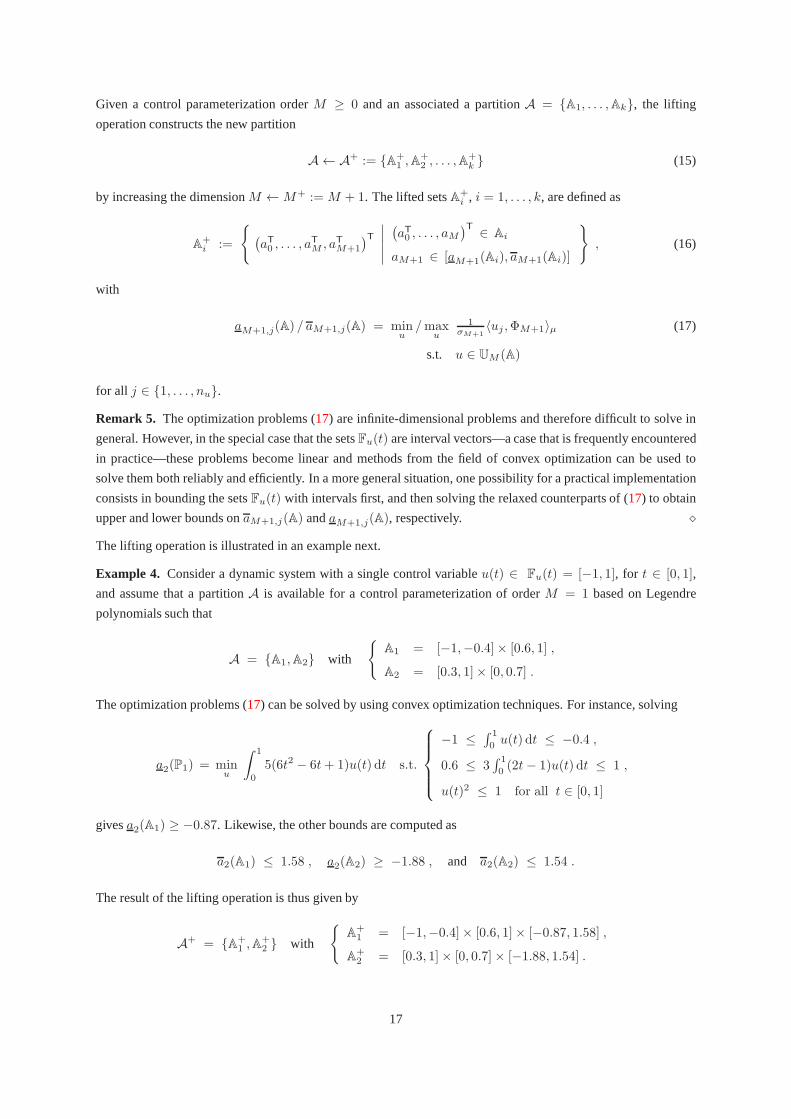
Example 4. Consider a dynamic system with a single control variableu(t) ∈ Fu(t) = [−1, 1], for t ∈ [0, 1],
and assume that a partitionA is available for a control parameterization of orderM = 1 based on Legendre
polynomials such that
A = {A1,A2} with
{
A1 = [−1,−0.4]× [0.6, 1] ,
A2 = [0.3, 1]× [0, 0.7] .
The optimization problems (17) can be solved by using convex optimization techniques. Forinstance, solving
a2(P1) = minu
∫ 1
0
5(6t2 − 6t+ 1)u(t) dt s.t.
−1 ≤∫ 1
0 u(t) dt ≤ −0.4 ,
0.6 ≤ 3∫ 1
0 (2t− 1)u(t) dt ≤ 1 ,
u(t)2 ≤ 1 for all t ∈ [0, 1]
givesa2(A1) ≥ −0.87. Likewise, the other bounds are computed as
a2(A1) ≤ 1.58 , a2(A2) ≥ −1.88 , and a2(A2) ≤ 1.54 .
The result of the lifting operation is thus given by
A+ = {A+1 ,A
+2 } with
{
A+1 = [−1,−0.4]× [0.6, 1]× [−0.87, 1.58] ,
A+2 = [0.3, 1]× [0, 0.7]× [−1.88, 1.54] .
17

The left plot in Figure2 shows the original setsA1 andA2, while the right plot shows the lifted setsA+1 andA+
2 .
Essentially, the lifting step uses bounds on the control parameterization coefficientsa0 anda1 in order to determine
bounds on the following coefficienta2 in a control parameterization of orderM = 2. Clearly, it depends on the
particular geometry of the setsA1 andA2 as well as of the setFu how tight the bounds ona2 will be in the lifted
setsA+1 andA+
2 . In this example, the width ofA+1 along thea2-axis turns out to be smaller than that ofA+
2 . ⋄
Figure 2: Visualization of the lifting operation.Left plot: SetsA1 andA2 on the(a0, a1)-space.Right plot:LiftedsetsA+
1 andA+2 in the(a0, a1, a2)-space.
The lifting step satisfies the following invariance property by construction.
Proposition 4. LetA be a compact set and denote byA+ its lifted counterpart. Then,UM (A) = UM+1(A+)
and, accordingly,V∗M (A) = V∗
M+1(A+).
It is important to be aware of the fact that the width of a lifted setA+ may be larger than the width of its parent set
A. Nonetheless, the width of the setsA is uniformly bounded by the constantα that was introduced in Lemma1.
Proposition 5. Let Assumption1 and the blanket assumption A3 be satisfied. Let alsoα <∞ denote the constant
introduced in Lemma1. Then, for any compact setA, the width of the interval[aM+1,j(A), aM+1,j(A)] generated
by a lifting operation is bounded byα, i.e., we have
∀j ∈ {1, . . . , nu} aM+1,j(A) − aM+1,j(A) ≤ α.
Proof. The statement of the proposition follows immediately from Lemma1 and by definition of the lifting oper-
ation.
5.3 Branch-and-Lift Algorithm
The branch-and-lift algorithm is given in Algorithm 3 and detailed subsequently. The branching and fathoming
operations are the same as those defined earlier in Sect.3.3with the only difference that the boundsLM (A) and
UM (A) are now used instead ofLM (A) andUM (A).
Initialization The branch-and-lift algorithm starts withM = 0. In the case thatΦ0(t) = 1, for instance, this
corresponds to a constant control parameterization. The motivation here is that even a coarse parameterization
might already lead to the exclusion of certain parts of the control region that cannot contain any global optima.
18

Algorithm 3: Branch-and-lift algorithm for global optimal control
Input: Termination toleranceε > 0; Lifting parameter > 0
Initialization:
1. SetM = 0 andA = {A0}, with A0 ⊇ D0 being an interval.
Repeat:
2. Select an intervalA ∈ A.
3. Compute upper and lower boundsLM (A) ≤ V∗M (A) ≤ UM (A) using Algorithm 2.
4. Apply a fathoming operation.
5. If(
minA∈A UM (A)−minA∈A LM (A))
≤ ε orA = ∅, stop.
6. If the condition
maxA∈A
diam(
Y (t,A)⊕ EM (t,A))
≤ (1 + ) maxA∈A
diam (EM (t, {mid(A)})
holds for allt ∈ [0, T ], apply a lifting operation forM ←M + 1.
7. Apply a branching operation, and return to step2.
Output: Lower and upper boundsminA∈A LM (A) ≤ V ≤ minA∈A UM (A), or a proof of infeasibility.
A possible way of initializing the partitionA = {A0} is by noting that the interval[a0(∅), a0(∅)], as defined
in (17), encloses all possible values of the constant parameterization coefficienta0.
Lifting Condition Because branch-and-bound search is most efficient when the control parameterization order
M is small, the branch-and-lift strategy is to increaseM as infrequently as possible. Intuitively, it is desirable
to apply a lifting operation whenever the error associated with the control parameterization becomes of the same
order of magnitude as the reachable set of the original ODE (8) itself. The former can be evaluated as the diameter
ofEM (t, {mid(A)}) as computed at the midpoint ofA, whereas the later can be over-approximatedas the diameter
of the setY (t,A)⊕ EM (t,A) . This leads to the following lifting condition:
∀t ∈ [0, T ] (18)
maxA∈A
diam(
Y (t,A)⊕ EM (t,A))
≤ (1 + ) maxA∈A
diam (EM (t, {mid(A)})) ,
where > 0 is a tuning parameter. Finite termination of the branch-and-lift algorithm based on the lifting
condition (18) is investigated in Sect.5.4.
In the branch-and-lift algorithm, the decision whether to perform a normal branching or to apply a lifting operation
before branching based on (18) is taken at each iteration. Moreover, a lifting operation is appliedglobally to all of
the parameter subsets in a current partitionA; that is, all the subsets inA share the same parameterization order, at
any iteration. As a variant of the branch-and-lift algorithm given in Algorithm 3, one could also imagine a family
of subsets that would have different parameterization orders by applying the lifting condition locally instead.
5.4 Finite Termination of Branch-and-Lift Algorithms
In this section, we investigate conditions under which Algorithm 3 finds anε-suboptimal solution of the optimal
control problem (1) after a finite number of iterations. The following assumptions on the convergence of the
enclosure functionsY (t, ·) andEM (t, ·) are introduced to carry out the analysis.
19

Assumption 2. There exists a constantCY <∞ such that
diam(
Y (t,A))
≤ CY diam(A) (19)
for all setsA with a sufficiently small diameterdiam(A).
Assumption 3. There exist constantsC0E∈ R, C1
E∈ R++ andC2
E∈ R+ such that
diam (EM (t, {mid (A)})) ≤ exp(
C0E − C1
EM)
and (20)
diam (EM (t,A)) ≤ diam(EM (t, {mid (A)})) + C2E diam (A) (21)
for all compact setsA and for allM ∈ N.
Note that Assumption2 is automatically satisfied if standard tools from interval arithmetics are applied to
bound the state trajectoryy(t, a), since the functiony(t, ·) is Lipschitz continuous. On the other hand, Assump-
tion 3 requires that the bounds on the image setEM (t, a) inherit the exponential convergence property established
in Theorem1. In particular, this assumption is satisfied by applying thebounding procedure described in Ap-
pendixB.
In order to simplify the convergence argumentation, the case without state constraints, i.e.Fx(t) = Rnx , is
addressed first.
Lemma 2. Let Assumptions2 and3 as well as the blanket assumptions A1, A2 and A4 be satisfied, and suppose
thatFx(t) = Rnx . Then, for any finite toleranceε > 0, Algorithm 3 applies at most
M =
⌈
1
C1E
(
log
(
LΨ(1 + )
ε
)
+ C0E
)⌉
(22)
lifting steps, whereLΨ <∞ stands for the Lipschitz constant of the Mayer termΨ.
Proof. Let A be any compact set. SinceFx(t) ⊖ EM (t,A) = Rnx , we either haveUM (A) = LM (A) = ∞, or
we have
UM (A)− LM (A) ≤ LΨ diam(
Y (T,A)⊕ EM (T,A))
. (23)
The former can only occur ifA∩DM = ∅, in which case the setA would be fathomed by Algorithm 3. Therefore,
a lifting is only applied if
UM (A)− LM (A) ≤ LΨ(1 + ) maxA∈A
diam (EM (T, {mid (A)}))
≤ LΨ(1 + ) exp(C0E − C1
EM) ,
which follows by substituting the lifting condition (18) in (23). SinceLΨ(1 + ) exp(C0E− C1
EM) can be made
as close to zero as desired by increasingM and is independent ofA, there existsM <∞ such that
UM (A)− LM (A) ≤ ε ,
for every compact setA with A ∩ DM 6= ∅. In particular, (22) yields an upper bound on the number of lifting
steps applied by Algorithm 3.
20

Observe that Lemma2 provides an upper bound on the number of lifting operations applied by Algorithm 3 for
a given toleranceε > 0, but it does not establish finite termination of Algorithm 3.This result is established in
the following theorem, under the additional assumption that the branching operation is exhaustive for every given
parameterization orderM .
Theorem 2. Let Assumptions2 and3 as well as the blanket assumptions A1, A2 and A4 be satisfied, and suppose
thatFx(t) = Rnx . If the branching operation is exhaustive for every given parameterization orderM ∈ N, then
Algorithm 3 terminates finitely for any finite toleranceε > 0 and any lifting parameter > 0.
Proof. By contradiction, assume that Algorithm 3 does not terminate finitely. From Lemma2, the maximum
numberM∗ of lifting operations applied by Algorithm 3 is such thatM∗ ≤ M ; that is,M∗ is attained after
a finite number of branching operations, and the algorithm then keeps branching forever, so that the following
conditions remain satisfied for an infinite number of iterations:
A 6= ∅ and ε < minA∈A
UM∗(A)−minA∈A
LM∗(A) .
By Assumptions2 and3, it follows that
ε(23)< LΨ max
A∈Adiam
(
Y (T,A)⊕ EM∗(T,A))
≤ maxA∈A
LΨ(CY + C2E ) diam (A) + LΨ max
A∈Adiam (EM∗(T, {mid(A)})
≤ maxA∈A
LΨ(CY + C2E ) diam (A) + LΨ exp(C0
E − C1EM
∗) .
Since the branching operation is exhaustive for any parameterization orderM , in particularM∗, we have that
diam (A) = 0 in the limit and therefore
ε ≤ LΨ exp(C0E − C1
EM∗) ≤ LΨ exp(C0
E − C1EM)
(22)≤
ε
1 + .
Finally, since the inequalityε ≤ ε1+ cannot be satisfied for bothε > 0 and > 0, we obtain a contradiction.
While Theorem2 is based solely on assumptions that are verifiablea priori, the situation becomes more involved
as soon as general state constraints are present. This is because the upper-bounding problem can fail to determine
a finite upper bound within a finite number of branch-and-liftiterations with such constraints. Nonetheless, this
problem is not specific to the proposed branch-and-lift algorithm, but it is a known problem of branch-and-bound
in general, as discussed in [29, 34, 35].
In the following two subsections, we analyze the finite convergence of Algorithm 3 in the presence of state con-
straints under the additional condition that either a particular constraint qualification holds, or a reliable (local)
optimal control solver is available.
5.4.1 Finite Termination with General State Constraints via a Constraint Qualification
A guarantee of finite termination with Algorithm 3 in the presence of general state constraints can be obtained
by enforcing a certain constraint qualification. The following assumption is similar in essence to the constraint
qualification imposed by Bhattacharjee et al. [10] in the context of semi-infinite programming.
21

Assumption 4. The optimal control problem(1) is strictly feasible in the sense that there exists a sequence of
feasibleL2-integrable functions{ui}i∈N such that
limi→∞
maxt∈[0,T ]
‖ui(t)− u∗(t) ‖ = 0 and
∀(t, i) ∈ [0, T ]× N
{
ui(t) ∈ Fu(t)
x(t, ui) ∈ int (Fx(t)) .
for at least one global minimizeru∗ of (1), whereint (Fx(t)) denotes the interior of the setFx(t).
It is important to note that such a constraint qualification fails to hold for many optimal control problems in
practice. In the case of optimal control problems with terminal equality constraints, for instance, one has
int(Fx(T )) = ∅. Nonetheless, the following finite-termination result canbe established under this assump-
tion.
Corollary 1. Let Assumptions2, 3 and4 as well as the blanket assumptions A1, A2, A3 and A4 be satisfied. If the
branching operation is exhaustive for every given parameterization orderM ∈ N, then Algorithm 3 terminates
finitely.
Proof. Assumption4 implies that there exists a feasibleε-suboptimal solutionu∗ε ∈ L2[0, T ]nu of (1) satisfying
x(t, u∗ε) ∈ int(Fx(t)) for all t ∈ [0, T ]. Sincediam (EM (t,A)) converges to zero forM →∞ anddiam(A)→ 0
(Assumption3), it follows that for all sufficiently largeM <∞ and all sufficiently smallδ > 0 we have
Y (t,A) ⊆ Fx(t)⊖ EM (t,A)
for all compact setsA satisfyingdiam (A) ≤ δ and
(
〈u∗ε,Φ0〉
T
µ , . . . , 〈u∗ε,ΦM 〉
T
µ
)T
∈ A .
ConsequentlyUM (A) < ∞ for all sufficiently small setsA contained in a small neighborhood of the Gram-
Schmidt projection ofu∗ε, thereby allowing us to transfer the proofs of Lemma2 and Theorem2 line by line to
arrive at the result.
5.4.2 Finite Termination with General State Constraints based on a Reliable Local Optimal Control Solver
An alternative way of obtaining a guarantee of finite termination with Algorithm 3, which removes the need for
the constraint qualification in Assumption4, is by assuming that a reliable local optimal control solveris available,
as defined next.
Definition 2. An optimal control solver is said to belocally reliablefor the problem(1) under a given control
parameterization{Φi}i∈N if, for all M ∈ N, there existsδ > 0 such that this solver returns a feasible solution of
problem(12) for all compact setsA with diam(A) ≤ δ andV ∗M (A) <∞.
Unfortunately, currently available implementations of local optimal control solver do not come along with such
local reliability guarantees and may fail to find feasible solutions for certain degenerate state constraint geometries,
such as optimal control problems having a single feasible point. It is our experience, however, that local optimal
control solvers work well for reasonably formulated, practical optimal control problems, when initialized in a
small neighborhood around the locally optimal solution. The following finite-termination result hold under the
assumption that a reliable local optimal control solver is available.
22

Corollary 2. Let the optimal control problem(1) be feasible, and suppose that a reliable local optimal control
solver is available. For any compact setA ∈ A with diam (A) ≤ δ andV ∗M (A) <∞, let the inner-approximation
functionY (·,A) be obtained as
∀t ∈ [0, T ] Y (t,A) :={
y(
t,(
〈u,Φ0〉T
µ , . . . , 〈u,ΦM 〉T
µ
)T)}
,
whereu is a feasible solution of(12). Let also Assumptions2 and3 as well as the blanket assumptions A1, A2,
A3 and A4 be satisfied. If the branching operation is exhaustive for every given parameterization orderM ∈ N,
then Algorithm 3 terminates finitely.
Proof. The proof of this statement is analogous to the proof of Theorem2 to the only difference that the conver-
gence of the upper bound is now guaranteed by the assumption of a reliable local optimal control solver.
As already mentioned, neither Corollary1 nor Corollary2 are entirely satisfactory in that they rely on rather strong
assumptions, which are not always satisfied in practice and are difficult to checka priori. We reiterate that similar
problems can arise for finite-dimensional NLP problems too if suitable constraint qualifications fail to hold or if
a reliable local solver is unavailable [29, 34, 35]. As such, the development of optimal control solvers that would
come along with local reliability guarantees under preferably mild constraint qualifications remains an important
topic for future research.
Finally, we consider the more general case that the functionsf andG in (1) are locally, but not globally, Lipschitz
continuous; that is, the solution trajectoriesx(t, u) andy(t, a) may not exist on all of[0, T ] for certain choices
of u anda due to the presence of a finite escape time. We start by noting that state-of-the-art enclosure methods
for nonlinear ODEs can validate existence and uniqueness ofthe solutions [47], thereby potentially providing a
mechanism to fathom control regions in which the ODEs have nosolutions. But regardless, a formal proof of
convergence of the branch-and-lift algorithm can still be obtained under the weaker assumptions thatf andG are
smooth, yet not necessarily globally Lipschitz continuous. Specifically, the results in Theorem2 and Corollaries1
and2 hold upon replacing the blanket assumption A2 with
A2’: The functionsf : Rnx → Rnx andG : Rnx → Rnx×nu are smooth, and there existsδ > 0 and a global
minimizeru∗ of the optimal control problem (1) such that the differential equation (8) admits a solutionx(t, u)
for all u ∈ L2[0, T ]nu with∫ T
0 ‖u(t)− u(t∗)‖2 dt ≤ δ.
and modifying Assumptions2 and3 so that (19)–(21) hold in a local neighborhood ofu∗. This extension is a
direct consequence of the fact that, under Assumption A2’, the solution trajectoriesx(·, u) andy(·, a), and in
turn the enclosure functionsY (·,A) andEM (·,A), are guaranteed to exist for sufficiently large parameterization
ordersM in a neighborhood ofu∗.
6 Numerical Case Study: Optimal Control of a Bioreactor
Rather than providing a detailed numerical implementationor performance assessment of the branch-and-lift algo-
rithm, the objective of this section is to demonstrate its application on a practical case study. Our implementation
of Algorithm 3 is based on the ACADO Toolkit [31] as the local optimal control solver—see Sect.5.4.2—and
uses the library MC++ [45] to compute the required nonlinearity bounds as well as the ODE enclosures based on
Taylor models combined with rigorous remainder estimates [58].
The fermentation control problem considered in this case study is based on a process model that has been devel-
oped in [52, 54]. The dynamics are highly nonlinear and several operational strategies have been reported in the
23

literature [3, 32, 54]. To the authors’ best knowledge, however, the applicationof a generic deterministic global
optimization algorithm to findε-suboptimal solutions has never been attempted for this problem.
Problem Definition Consider a continuous culture fermentation process described by the following dynamic
model [3, 52, 54]:
f(x) =
− 1T Dx4
−Dx2 + µ(x3, x4)x2
−Dx3 −µ(x3,x4)x2
YX/S
−Dx4 + (αµ(x3, x4) + β)x2
0
and G(x) =
0
0
D
01T
,
with
µ(x3, x4) = µm
(
1− x4
Pm
)
x3
Km + x3 +x23
Ki,
and the initial value
x(0) = (0 , X0 , S0 , P0 , 0)T.
The Mayer term in this problem isΨ(x) = x1 and the set of feasible states is given by
∀t ∈ [0, T ) Fx(t) = R5 , and Fx(T ) =
x ∈ R5
∣
∣
∣
∣
∣
∣
∣
∣
∣
∣
∣
x2 = X0
x3 = S0
x4 = P0
x5 = S f
.
Moreover, the feasible control set is
∀t ∈ [0, T ] Fu(t) :={
u | Sminf ≤ u ≤ Smax
f
}
,
and an isoperimetric constraint on the control input is defined such that
a0 =
∫ T
0
u(t) dt = S f
(wherea0 is the first coefficient in a control parameterization based on Legendre polynomials.) All of the model
parameters are reported in Table1.
Optimal Control Solution Figure3 displays the optimal control and response for anε-optimal solution, as
determined by the proposed branch-and-lift algorithm withoptimality toleranceε = 0.001 g h−1 L−1. We find
that this solution is identical to the one found in [32] by using local search methods, with some good insight on
how to initialize the search. A major difference here is thatthe branch-and-lift algorithm comes along with a
certificate that the computed solution is within0.001 g h−1 L−1 of the actual global solution.
Discussion The focus of the ensuing discussion is on the performance of the branch-and-lift algorithm (Algo-
rithm 3). The control parameterization at the start of the algorithm being rather coarse, we find that two lifting
operations are applied during the first two branch-and-liftiterations; that is, the lifting condition (18) happens to
24

Table 1: Fermentation process parametersDescription Symbol Valuedilution rate D 0.15 h−1
substrate inhibition constant Ki 22 g L−1
substrate saturation constant Km 1.2 g L−1
product saturation constant Pm 50 g L−1
yield of the biomass YX/S 0.4first product yield constant α 2.2second product yield constant β 0.2 h−1
specific growth rate scale µm 0.48 h−1
average feed substrate concentration S f 32.0 g L−1
minimum feed substrate concentration Sminf 28.0 g L−1
maximum feed substrate concentrationSmaxf 40.0 g L−1
duration of one period T 48 hbiomass initial condition X0 6.9521 g L−1
substrate initial condition S0 13.4166 g L−1
product initial condition P0 24.1566 g L−1
be satisfied forM = 0 andM = 1 without branching. As the parameterization order is increased toM = 2,
however, the algorithm performs a number of branching operations and the fathoming test successfully excludes
a number of suboptimal control regions. The projection ontothe (a1, a2)-plane of the partitionA at the order
M = 2 is shown as the grey-shaded area on the left plot in Figure4—recall thata0 = S f due to the isoperimetric
constraint. The intervals[a1, a1] and[a2, a2] reported on this plot are those computed during the first and second
lifting steps, and the unshaded part of the box[a1, a1] × [a2, a2] shows the control subregion that is excluded
before the third lifting step—i.e., fromM = 2 to M = 3—is applied. Represented on the right plot in Figure4
are the projections onto the(a1, a2)-plane of the partitionA before the third, fourth, fifth and sixth lifting steps,
with darker grey shades corresponding to more refined control parameterizations. Observe, in particular, how the
region in which the globally optimal control coefficientsa1 anda2 belong progressively shrinks as the control
parameterization is refined.
The left plot in Figure5 displays the cardinality of the partitionA immediately before the next lifting operation
is applied, here for parameterization ordersM = 2, . . . , 7. Notice that the partition size remains rather small,
between 100-200 subsets, and it even decreases for largerM . The right part of Figure5 shows the decrease in
the optimality gap(minA∈A UM (A) −minA∈A LM (A)) between the upper and the lower bound on the optimal
valueV as the parameterization orderM is increased, until the desired toleranceε is attained.
In this case study, Algorithm 3 stops after810 iterations, taking approximately2.5 hours to converge and finding
the solution that is displayed in Figure3.
7 Conclusions
This paper has presented a new branch-and-lift algorithm for solving nonlinear optimal control problems with
smooth nonlinear dynamics and nonconvex objective and constraints to guaranteed global optimality. Particular
emphasis has been on the convergence properties of the imageof the control parameterization error in state space,
which are summarized in Theorem1. Another principal contribution of this paper has been the introduction of a
lifting operation in Sect.5, which adapts the control parameterization accuracy during the global search. The most
important result of this paper is that the proposed branch-and-lift algorithm can findε-suboptimal solutions of the
continuous-time optimal control problem (1) in a finite number of iterations, as proven in Theorem2 as well as
25

Figure 3: The state trajectories “X = x2”, “ S = x3”, and “P = x4” as well as the control trajectory “Sf = u”corresponding to anε-optimal solution of the fermentation process case study, with accuracyε = 0.001 g h−1 L−1.
Corollaries1 and2. As far as the authors are aware, this algorithm is the first complete search method of its kind,
apart from algorithms based on dynamic programming. Finally, the performance of the proposed branch-and-lift
algorithm has been illustrated for the optimal control of a periodic fermentation process.
Appendix A Proof of Theorem 1
The aim of this section is to construct convergent bounds on the setEM (t, a), thereby providing a proof of
Theorem1. Recall the definition of the setEM (t, a) in Sect.4 as
EM (t, a) := {x(t, u)− y(t, a) |u ∈ UM (a) } .
Also recall the blanket assumption A2, which guarantees that the solution trajectoriesx andy are well-defined, so
that a sufficiently large and compacta priori enclosureE ⊆ Rnx can always be found such that
∀t ∈ [0, T ] EM (t, a) ⊆ E .
The focus here is on tightening thea priori enclosureE, which is crucial for analyzing the convergence of the set
EM (t, a). We start by defining the response defect
d(t, u, a) = x(t, u)− y(t, a) ,
26

Figure 4: Left plot: Projection of the partitionA onto the(a1, a2)-plane (grey shaded area) before the third liftingstep is performed. Right plot: Projection of the partitionA onto the(a1, a2)-plane before the third, fourth, fifthand sixth lifting steps, i.e., forM ∈ {2, 3, 4, 5}.
which by construction satisfies an ODE of the form
∀t ∈ [0, T ]
d(t, u, a)(3),(8)= f(x(t, u))− f(y(t, a)) +G(x(t, u))u(t) −G(y(t, a))
(
M∑
i=0
aiΦi(t)
)
(24)
with d(0, u, a) = 0 .
In order to bound the solution trajectory of (24), consider a Taylor expansion of the termf(x(t, u)) − f(y(t, a))
in the form
f(x(t, u))− f(y(t, a)) =∂f(y(t, a))
∂xd(t, u, a) + Rf (t, u, a)d(t, u, a) ,
where the matrixRf (t, u, a) ∈ Rnx×nx denotes a nonlinear remainder term. By the mean-value theorem,Rf is
bounded as
∀u ∈ UM (a) ‖Rf(t, u, a)‖ ≤ maxd′,d′′∈E
∥
∥
∥
∥
1
2
∂2f(y(t, a) + d′)
∂x2d′′∥
∥
∥
∥
. (25)
Similarly, the mean-value theorem can be applied to the term[G(x(t, u)) −G(y(t, a))] u(t), giving
[G(x(t, u))−G(y(t, a))]u(t) = RG(t, u, a)d(t, u, a) ,
where the nonlinear remainder termRG(t, u, a) is bounded by
∀u ∈ UM (a) ‖RG(t, u, a)‖ ≤ maxu′∈Fu(t)
maxd′∈E
∥
∥
∥
∥
∂G(y(t, a) + d′)
∂xu′
∥
∥
∥
∥
. (26)
27

Figure 5: Left: The number of boxes in the set familyA for M = 2, . . . , 7 before applying the next lifting step.Right: The gap between upper and lower bound forM = 1, 2, . . . , 7.
In the following, we introduce the shorthand notationR(t, u, a) := Rf (t, u, a) + RG(t, u, a), so that (24) can be
written in the form
∀t ∈ [0, T ]
d(t, u, a) =∂f(y(t, a))
∂xd(t, u, a) +R(t, u, a)d(t, u, a) +G(y(t, a))
[
u(t)−
M∑
i=0
aiΦi(t)
]
(27)
with d(0, u, a) = 0 .
A few remarks are in order regarding the previous ODE (27).
1. The Jacobian off and the functionG are evaluated at the pointy(t, a). Therefore, these matrices are
independent of the control inputu.
2. The matrix-valued remainder termR(t, u, a) depends onu in general, but standard tools such as interval
arithmetics can be applied to construct a boundR(t, a) <∞ independent ofu such that:
∀t ∈ [0, T ]
maxd′,d′′∈E
∥
∥
∥
∥
∂2f(y(t, a) + d′)
∂x2
d′′
2
∥
∥
∥
∥
2
+ maxu′∈Fu(t)
maxd′∈E
∥
∥
∥
∥
∂G(y(t, a) + d′)
∂xu′
∥
∥
∥
∥
2
≤ R(t, a) . (28)
The validity of this bound follows from the inequalities (25) and (26):
∀u ∈ UM (a) ‖R(t, u, a)‖2 ≤ R(t, a) .
However, the tightness of the boundR(t, a) depends strongly on the tightness of thea priori enclosureE,
and a tighterE will typically lead to a tighter bound on the norm of the remainder termR.
28

3. The right-hand side of the ODE (27) also depends on the control parameterization defect(u−∑M
i=0 aiΦi).
It follows by orthogonality of theΦi’s that the firstM + 1 Gram-Schmidt coefficients of this defect are
all equal to zero. Consequently, an enclosureWM (a) of the control parameterization defect, which is
independent ofu and convex (Assumption A4), is obtained as:
∀u ∈ UM (a)
u−M∑
i=0
aiΦi ∈ WM (a) :=
w ∈ L2[0, T ]nu
∣
∣
∣
∣
∣
∣
∣
∣
∣
∣
∣
∀i ∈ {0, . . . ,M}, ∀t ∈ [0, t]
0 = 〈w,Φi〉µ
w(t) +
M∑
i=0
aiΦi(t) ∈ Fu(t)
. (29)
Summarizing the above considerations, the main idea is to regard the solution trajectory of the differential equa-
tion (27) as a function of the remainder term and of the control parameterization defect rather than as a function of
the control functionu. In order to formalize this change of variable, lete(t,∆, w) denote the solution of the ODE
e(t,∆, w) = [A(t) + ∆(t)] e(t,∆, w) +B(t)w(t) with e(0,∆, w) = 0, (30)
for any functionsw ∈ L2[0, T ]nu and∆ ∈ L2[0, T ]nx×nx , where we have introduced the shorthand notations
A(t) := ∂f(y(t,a))∂x andB(t) := G(y(t, a)).
Proposition 6. LetR(·, a) be a remainder bound satisfying(28), and letWM (a) be defined by(29). Then,
∀(t, a) ∈ [0, T ]× DM EM (t, a) ⊆
e(t,∆, w)
∣
∣
∣
∣
∣
∣
w ∈WM (a)
∀τ ∈ [0, T ] ‖∆(τ)‖2 ≤ R(τ, a)
,
wheree(·,∆, w) denotes the solution of(30).
Proof. From the definition of the defect functiond, we have
EM (t, a) = { d(t, u, a) |u ∈ UM (a) } .
Moreover, the functione is defined such that
d(t, u, a) = e
(
t, R(·, u, a), u−
M∑
i=0
aiΦi
)
.
Therefore, the result of the proposition follows by applying the change of variables
R(·, u, a) → ∆ and u−M∑
i=0
aiΦi → w
and using thatR(·, a) andWM (a) are bounds on the norm of the remainder term and on the controlparameteri-
zation defect, respectively.
In order to understand the motivation behind Proposition6, it is helpful to interpret the differential equation (30)
as a low-pass filter with uncertain but bounded gain∆, which would filter high-frequency modes of the “noise”
w. This interpretation is useful, as the control parameterization defectw = u−∑M
i=0 aiΦi is bounded by the set
WM (a). For example, ifΦ0,Φ1, . . . denote the basis functions in a standard trigonometric Fourier expansion, the
29

setWM (a) contains for largeM only highly oscillatory functions, as the firstM + 1 Fourier coefficients of the
control parameterization are zero in this case. The differential equation (30) can be expected to filter out these
highly oscillating modes such thate(t,∆, w) ≈ 0. Having this interpretation in mind, intuition suggests that we
should be able to compute tight bounds on the functione(t,∆, w), which converge forM → ∞, even when the
uncertain gain∆ is not known exactly.
The aim of the following considerations is to formalize thisintuition by translating it into a rigorous algorithm that
computes convergent enclosures of the setsEM (·, a) on [0, T ]. To do so, the functione(t,∆, w) is decomposed
into the sum of two functionseL(t, w) andeN(t,∆, v), such that
e(t,∆, w) = eL(t, w) + eN(t,∆, eL(·, w)).
Specifically,eL(·, w) is the solution of the auxiliary filter equation with inputw and known gain
∀t ∈ [0, T ] eL(t, w) = A(t)eL(t, w) +B(t)w(t) with eL(0, w) = 0 , (31)
whereaseN(·,∆, v) is the solution of the auxiliary filter equation with inputv and unknown gain∆
∀t ∈ [0, T ] eN(t,∆, v) = (A(t) + ∆(t)) eN(t,∆, v) + ∆(t)v(t) with eN(t,∆, v) = 0 . (32)
Moreover, the outputeL of the first filter (31) becomes an input in the second filter (32), before adding both outputs
eL andeU to yielde. We also define the sets
ELM (t, a) := { eL(t, w) |w ∈WM (a) }
and ENM (t, a) :=
eN(t,∆, v)
∣
∣
∣
∣
∣
∣
∀τ ∈ [0, t]v(τ) ∈ EL
M (τ, a)
‖∆(τ)‖2 ≤ R(τ, a)
.
The following proposition is a direct consequence of Proposition 6 and of the decomposition of the functione.
Proposition 7. The image setEM (t, a) is contained in the Minkowski sum of the setsELM (t, a) andEN
M (t, a),
∀(t, a) ∈ [0, T ]× DM EM (t, a) ⊆ ELM (t, a)⊕ EN
M (t, a) . (33)
In order to find a convergent bound on the diameter of the setEM (t, a), it is sufficient to find a convergent bound
on the diameter of the setELM (t, a), as stated in the following lemma.
Lemma 3. There exists a constantℓ(t) <∞ such that
∀t ∈ [0, T ] diam (EM (t, a)) ≤ ℓ(t) maxτ∈[0,T ]
diam(
ELM (τ, a)
)
.
Proof. Since the uncertain gain∆ is bounded, there exist constantsℓ1 andℓ2 such that
‖A(t) + ∆(t)‖2 ≤ ℓ1 and ‖∆(t)v(t)‖2 ≤ ℓ2diam
(
ELM (t, a)
)
2
for all v with v(t) ∈ ELM (t, a), all ∆ with ‖∆(t)‖2 ≤ R(t, a), and allt ∈ [0, T ]. Applying Gronwall’s lemma
for bounding the norm of the solution of the differential equation (32) yields the following bound on the diameter
30

of ENM (t, a):
diam(
ENM (t, a)
)
≤ exp (ℓ1t) ℓ2 maxτ∈[0,T ]
diam(
ELM (τ, a)
)
.
It then follows from Proposition7 that
diam (EM (t, a)) ≤ diam(
ELM (t, a)
)
+ diam(
ENM (t, a)
)
≤ [1 + ℓ2 exp (ℓ1t)] maxτ∈[0,T ]
diam(
ELM (τ, a)
)
(34)
and the result follows by definingℓ(t) := 1 + ℓ2 exp (ℓ1t).
The focus in the remainder of this appendix is on bounding thesetELM (t, a). We start by noting that the image
setsELM (t, a) are compact and convex. The compactness ofEL
M (t, a) follows from Filippov’s theorem [23].
Moreover, the convexity ofELM (t, a) follows from the fact that linear transformations of convexsets are convex,
recalling that the setWM (a) is convex and that the functionaleL(t, ·) is linear since the ODE (31) is itself linear
(see also [4]). Because any compact and convex set is uniquely characterized by its support function [15], we
define the support functionV (t, ·) : Rnx → R associated with the image setELM (t, a) by
∀c ∈ Rnx V (t, c) := maxw∈WM (a)
cTeL(t, w) . (35)
The following inequality
diam(
ELM (t, a)
)
≤ 2 supc
V (t, c)
‖c‖2,
follows directly from (35) and provides a means to bound the diameter ofELM (t, a). In expanded form,V (t, c)
reads
V (t, c) := maxw∈L2[0,T ]nu
cT∫ t
0
Z(t, τ)B(τ)w(τ) dτ s.t.
∀i ∈ {0, . . . ,M}, ∀t ∈ [0, t]
0 = 〈w,Φi〉µ
w(t) +
M∑
i=0
aiΦi(t) ∈ Fu(t),
(36)
whereZ : [0, T ]× [0, T ]→ Rnx×nx stands for the fundamental solution of the parametric linear ODE (31), which
satisfies
∀τ, t ∈ [0, T ]∂
∂tZ(t, τ) = A(t)Z(t, τ) with Z(τ, τ) = I .
Since the setsFu(t) are compact, one can always scale the dynamic system, and we shall therefore restrict the
analysis to thoseL2-integrable functionw with w(t) +∑M
i=0 aiΦi(t) ∈ Fu(t) for all t ∈ [0, T ] and such that
‖w‖µ,L2=
∫ T
0
w(t)Tw(t)µ(t) dt ≤ 1 .
Moreover, we introduce the functionsHt : [0, T ]→ Rnx×nx andθ : [0, T ]× [0, T ]→ R defined by
Ht(τ) :=1
µ(τ)Z(t, τ)B(τ)θ(t, τ) and θ(t, τ) :=
{
1 if τ ≤ t
0 otherwise,
31

for all t, τ ∈ [0, T ], so that the objective function in (36) can be written in the form
cT∫ t
0
Z(t, τ)B(τ)w(τ) dτ = cT∫ T
0
1
µ(τ)Z(t, τ)B(τ)θ(t, τ)w(τ)µ(τ) dτ =
⟨
cTHt , w⟩
µ.
With this notation, an upper bound on the support functionV (t, c) is given by
V (t, c) ≤ maxw
⟨
cTHt , w⟩
µs.t.
0 = 〈w,Φi〉µ for all i ∈ {0, . . . ,M}
‖w‖µ,L2≤ 1 .
(37)
Associating with each equality constraint0 = 〈w,Φi〉µ in (36) the scaled multiplierscTDi ∈ Rnu , the dual of the
convex problem (37) gives
V (t, c) ≤ infD
maxw
⟨
cTHt, w⟩
µ−
M∑
i=0
cTDi〈Φi, w〉µ s.t. ‖w‖µ,L2≤ 1
= infD
∥
∥
∥
∥
∥
cT
(
Ht −
M∑
i=0
DiΦi
)∥
∥
∥
∥
∥
µ,L2
=
∥
∥
∥
∥
∥
cT
(
Ht −
M∑
i=0
〈Ht,Φi〉µσi
Φi
)∥
∥
∥
∥
∥
µ,L2
. (38)
In the latter transformation, the tight version of the Cauchy-Schwarz inequality forL2-scalar products has been
applied. At this point, it becomes clear that the derived bound on the support functionV (t, c) depends crucially on
how accurately the functionHt can be approximated with the function∑M
i=0 DiΦi. This observation is formalized
in the following theorem.
Theorem 3. Let Assumption1 and the blanket assumptions A2 and A4 be satisfied. Then, there exist constants
CL,0E ∈ R andCL,1
E ∈ R++ such that the condition
∀(t, a) ∈ [0, T ]× DM log(
diam(
ELM (t, a)
) )
≤ CL,0E − CL,1
E M
is satisfied for allM ∈ N.
Proof. Since the functionHt is piecewise smooth and from Assumption1, there exists a sequenceD0, D1, . . . ∈
Rnx×nu as well as constantsC0H ∈ R andC1
H ∈ R++ such that
log
(∥
∥
∥
∥
∥
Ht(τ) −
M∑
i=0
DiΦi(τ)
∥
∥
∥
∥
∥
)
≤ C0H − C1
HM (39)
for almost allτ ∈ [0, T ] and for allM ∈ N. By combining (37) and (39), it follows that there exists a constant
Cµ ∈ R++ such that
log(
diam(
ELM (t, a)
) )
≤ log
(
2 supc
V (t, c)
‖c‖2
)
≤ 2Cµ
[
C0H − C1
HM]
(40)
for almost allτ ∈ [0, T ] and for allM ∈ N. In the last step, we have used the Lebesgue dominated convergence
theorem (or alternatively Fatou’s lemma), which guarantees that the Lebesgue zero measure of pointsτ ∈ [0, T ]
at which the inequality (39) may be violated does not contribute to the bound on theL2-norm of the function
Ht −∑M
i=0 DiΦi. The statement of the theorem follows by takingCL,0E := 2CµC
0H andCL,1
E := 2CµC1H .
Finally, a proof of Theorem1 is obtained by combining the results in Theorem3 and Lemma3.
32

Appendix B Practical Computation of Convergent EnclosuresEM(t,A)
Since the proof in AppendixA is essentially constructive, a line-by-line transcription of this proof into a
numerical bounding procedure that constructs an enclosureEM (t,A) satisfying Assumption3 is in principle
possible, assuming that suitable interval tools are available. For the implementation in this paper, we have used
the bounding and relaxation techniques available through the library MC++ [14, 45] and we have slightly refined
the procedure by exploiting the following observations:
1. From inequality (38), we know that the setELM (t, a) is enclosed by an ellipsoid of the formE(Q(t, a)) with
Q(t, a) :=
∫ T
0
(
Ht(τ) −
M∑
i=0
〈Ht,Φi〉µσi
Φi(τ)
)(
Ht(τ) −
M∑
i=0
〈Ht,Φi〉µσi
Φi(τ)
)T
dτ .
By using standard tools from interval analysis for differential equations, a convergent bounding matrix
Q(t,A) ∈ Rnx×nx can be constructed such thatQ(t, a) � Q(t,A) for all a ∈ A and allt ∈ [0, T ]. In
particular, if there exists a constantCQ such that
‖Q(t,A)−Q(t, {mid (A)}) ‖ ≤ CQ diam (A) ,
then the enclosureELM (t,A) := E(Q(t,A)) will satisfy the convergence conditions
log(
diam(
ELM (t, {mid (A)})
))
≤ CL,0E− CL,1
EM (41)
diam(
ELM (t,A)
)
− diam(
ELM (t, {mid (A)})
)
≤ CL,2E
diam(A) (42)
for all compact setsA and allM ∈ N and for some constantCL,0E∈ R, CL,1
E∈ R++ andCL,2
E∈ R+.
2. The proof of Lemma3 is based on Gronwall’s lemma, which is known to provide mathematically valid,
yet typically conservative, bounds for practical purposes. Instead, our implementation considers a modified
version of state-of-the art reachable set enclosure algorithms for bounding the solution of the differential
equation (32), which prove to be much less conservative than with Gronwall’s lemma.
Acknowledgements This paper is based upon work supported by the Engineering and Physical Sciences Re-
search Council (EPSRC) under Grant EP/J006572/1. Financial support from the Centre of Process Systems Engi-
neering (CPSE) of Imperial College is gratefully acknowledged.
References
[1] T. Achterberg, T. Koch, and A. Martin. Branching rules revisited. Oper. Res. Lett., 33:42–54, 2005.
[2] C. S. Adjiman, S. Dallwig, C. A. Floudas, and A. Neumaier.A global optimization method,αBB, for general
twice-differentiable constrained NLPs - I. Theoretical advances. Comput. Chem. Eng., 22(9):1137–1158,
1998.
[3] P. Agarwal, G. Koshy, and M. Ramirez. An algorithm for operating a fed-batch fermentor at optimum specific
growth rate.Biotechnol. Bioeng., 33:115–125, 1989.
33

[4] V. Azhmyakov and J. Raisch. Convex control systems and convex optimal control. IEEE Trans. Autom.
Contr., 53(4):993–998, 2008.
[5] J. R. Banga, C. G. Moles, and A. A. Alonso. Global optimization of bioprocesses using stochastic and
hybrid methods. In C. A. Floudas and P. M. Pardalos, editors,Frontiers in Global Optimization, volume 74
of Nonconvex Optimization and Its Applications, pages 45–70, Dordrecht, the Netherlands, 2003. Kluwer
Academic Publishers.
[6] R. E. Bellman.Dynamic Programming. Princeton University Press, Princeton, 1957.
[7] P. Belotti, J. Lee, L. Liberti, F. Margot, and A. Wachter. Branching and bounds tightening techniques for
non-convex MINLP.Oper. Res. Lett., 33:42–54, 2005.
[8] M. Berz and K. Makino. Performance of Taylor model methods for validated integration of ODEs.Lecture
Notes Comput. Sci., 3732:65–74, 2006.
[9] J. T. Betts.Practical Methods for Optimal Control Using Nonlinear Programming. Advances in Design and
Control Series. SIAM, Philadelphia, 2nd edition, 2010.
[10] B. Bhattacharjee, P. Lemonidis, W. H. Green, and P. I. Barton. Global solution of semi-infinite programs.
Math. Prog., Ser. B, 103(2):283–307, 2005.
[11] L. T. Biegler. Nonlinear Programming: Concepts, Algorithms, and Applications to Chemical Processes.
MOS-SIAM Series on Optimization. SIAM, Philadelphia, 2010.
[12] J. Bjornberg and M. Diehl. Approximate robust dynamicprogramming and robustly stable MPC.Automat-
ica, 42(5):777–782, 2006.
[13] H. G. Bock and K. J. Plitt. A multiple shooting algorithmfor direct solution of optimal control problems. In
Proc. IFAC 9th World Congress, pages 242–247, Budapest, Hungary, 1984.
[14] A. Bompadre, A. Mitsos, and B. Chachuat. Concergence analysis of taylor and mccormick-taylor models.
J. Global Optim., 35:844–857, in press, DOI:10.1007/s10898-012-9998-9.
[15] S. Boyd and L. Vandenberghe.Convex Optimization. University Press, Cambridge, UK, 2004.
[16] R. Brusch and R. Schappelle. Solution of highly constrained optimal control problems using nonlinear
programming.AIAA J., 11(2):135–136, 1973.
[17] A. E. Bryson and Y. Ho.Applied Optimal Control. Hemisphere, Washington D.C., 1975.
[18] B. Chachuat and M. A. Latifi. A new approach in deterministic global optimization of problems with ordinary
differential equations. In C. A. Floudas and P. M. Pardalos,editors,Frontiers in Global Optimization,
volume 74 ofNonconvex Optimization and Its Applications, pages 83–108, Dordrecht, the Netherlands,
2003. Kluwer Academic Publishers.
[19] B. Chachuat, A. B. Singer, and P. I. Barton. Global methods for dynamic optimization and mixed-integer
dynamic optimization.Ind. Eng. Chem. Res., 45(25):8373–8392, 2006.
[20] J. A. Egea, E. Vazquez, J. R. Banga, and R. M. Marti. Improved scatter search for the global optimization of
computationally expensive dynamic models.J. Global Optim., 43(2-3):175–190, 2009.
34

[21] W. R. Esposito and C. A. Floudas. Deterministic global optimization in nonlinear optimal control problems.
J. Global Optim., 17:96–126, 2000.
[22] W. R. Esposito and C. A. Floudas. Global optimization for the parameter estimation of differential-algebraic
systems.Ind. Eng. Chem. Res., 39(5):1291–1310, 2000.
[23] A. F. Filippov. On certain questions in the theory of optimal control. J. SIAM Control Ser. A, 1(1):76–84,
1962.
[24] A. Flores Tlacuahuac, S. Terrazas, and L. T. Biegler. Global optimization of highly nonlinear dynamic
systems.Ind. Eng. Chem. Res., 47(8):2643–2655, 2008.
[25] C. A. Floudas.Deterministic Global Optimization: Theory, Methods, and Applications. Kluwer Academic
Publishers, Dordrecht, the Netherlands, 1999.
[26] E. F. Galperin and Q. Zheng. Variation-free iterative method for global optimal control.Int. J. Control,
50(5):1731–1743, 1989.
[27] D. Gottlieb and C. W. Shu. On the Gibbs phenomenon and itsresolution.SIAM Rev., 39(4):644–668, 1997.
[28] L. Grune and W. Semmler. Using dynamic programming with adaptive grid scheme to solve nonlinear
dynamic models in economics.Computing in Economics and Finance 2002, (99), 2002.
[29] R. Horst. Deterministic global optimization with partition sets whose feasibility is not known: Application
to concave minimization, reverse convex constraints, DC-programming, and Lipschitzian optimization.J.
Optim. Th. Appl., 58(1):11–37, 1988.
[30] R. Horst and H. Tuy.Global Optimization: Deterministic Approaches. Springer-Verlag, Berlin, Germany,
3rd edition, 1996.
[31] B. Houska, H. J. Ferreau, and M. Diehl. ACADO Toolkit – Anopen source framework for automatic control
and dynamic optimization.Opt. Contr. Appl. Meth., 32(3):298–312, 2011.
[32] B. Houska, F. Logist, Y. van Impe, and M. Diehl. Approximate robust optimization of time-periodic sta-
tionary states with application to biochemical processes.In Proc. 50th IEEE Conf. Decision Control, pages
6280–6285, Shanghai, China, 2009.
[33] B. Houska, F. Logist, Y. van Impe, and M. Diehl. Robust optimization of nonlinear dynamic systems with
application to a jacketed tubular reactor.J. Process Contr., 22(6):1152–1160, 2012.
[34] R. B. Kearfott.Rigorous Global Search: Continuous Problems, volume 13 ofNonconvex Optimization and
Its Applications. Kluwer Academic Publishers, Dordrecht, the Netherlands,1996.
[35] R. B. Kearfott. On proving existence of feasible pointsin equality constrained optimization problems.Math.
Prog., 83:89–100, 1998.
[36] A. B. Kurzhanski and P. Valyi.Ellipsoidal Calculus for Estimation and Control. Birkhauser, Boston, MA,
1997.
[37] A. B. Kurzhanski and P. Varaiya. Reachability analysisfor uncertain systems – The ellipsoidal technique.
Dyn. Contin. Discret. Impulsive Sys., Ser. B, 9:347–367, 2002.
35

[38] J. B. Lasserre.Moments, Positive Polynomials and Their Applications. Imperial College Press, London, UK,
2009.
[39] D. B. Leineweber, I. Bauer, H. G. Bock, and J. P. Schloder. An efficient multiple shooting based reduced
SQP strategy for large-scale dynamic process optimization. Part I: Theoretical aspects.Comput. Chem. Eng.,
27:157–166, 2003.
[40] Y. Lin and M. A. Stadtherr. Deterministic global optimization of nonlinear dynamic systems.AIChE J.,
53(4):866–875, 2007.
[41] Y. Lin and M. A. Stadtherr. Validated solutions of initial value problems for parametric ODEs.Applied
Numer. Math., 57(10):1145–1162, 2007.
[42] R. Luss. Optimal control by dynamic programming using systematic reduction in grid size.Int. J. Control,
51(5):995–1013, 1990.
[43] R. Luss.Iterative Dynamic Programming. Chapman & Hall/CRC, Boca Raton, Florida, 2000.
[44] G. P. McCormick. Computability of global solutions to factorable nonconvex programs: Part I–Convex
underestimating problems.Math. Prog., 10:147–175, 1976.
[45] A. Mitsos, B. Chachuat, and P. I. Barton. McCormick-based relaxations of algorithms.SIAM J. Optim.,
20(2):573–601, 2009.
[46] A. Mitsos, B. Chachuat, and P. I. Barton. Towards globalbilevel dynamic optimization.J. Global Optim.,
45(1):63–93, 2009.
[47] N. S. Nedialkov, K. R. Jackson, and G. F. Corliss. Validated solutions of initial value problems for ordinary
differential equations.Appl. Math. Comput., 105(1):21–68, 1999.
[48] M. Neher, K. R. Jackson, and N. S. Nedialkov. On Taylor model based integration of ODEs.SIAM J. Numer.
Anal., 45:236–262, 2007.
[49] A. Neumaier. Complete search in continuous global optimization and constraint satisfaction.Acta Numerica,
13:271–369, 2004.
[50] C. P. Neuman and A. Sen. A suboptimal control algorithm for constrained problems using cubic splines.
Automatica, 9:601–603, 1973.
[51] I. Papamichail and C. S. Adjiman. A rigorous global optimization algorithm for problems with ordinary
differential equations.J. Global Optim., 24:1–33, 2002.
[52] S. J. Parulekar. Analysis of forced periodic operations of continuous bioprocesses - single input variations.
Chem. Eng. Sci., 53(14):2481–2502, 1998.
[53] L. S. Pontryagin, V. G. Boltyanskii, R. V. Gamkrelidze,and E. F. Mishchenko.The Mathematical Theory of
Optimal Processes. John Wiley & Sons, New York, 1962.
[54] L. Ruan and X. D. Chen. Comparison of several periodic operations of a continous fermentation process.
Biotechnol. Prog., 12:286–288, 1996.
[55] E. B. Saff and V. Totik. Polynomial approximation of piecewise analytic functions.J. London Math. Soc.,
39(2):487–498, 1989.
36

[56] N. V. Sahinidis. BARON: A general purpose global optimization software package.J. Global Optim.,
8(2):201–205, 1996.
[57] A. M. Sahlodin. Global Optimization of Dynamic Process Systems using Complete Search Methods. PhD
thesis, McMaster University, Ontario, Canada, 2012.
[58] A. M. Sahlodin and B. Chachuat. Convex/concave relaxations of parametric ODEs using Taylor models.
Comput. Chem. Eng., 35:844–857, 2011.
[59] A. M. Sahlodin and B. Chachuat. Discretize-then-relaxapproach for convex/concave relaxations of the
solutions of parametric ODEs.Applied Numer. Math., 61:803–820, 2011.
[60] R. W. H. Sargent and G. R. Sullivan. The development of anefficient optimal control package. In J. Stoer,
editor,Proc. 8th IFIP Conf. Optimization Techniques 1977, Heidelberg, 1978.
[61] J. K. Scott and P. I. Barton. Convex relaxations for nonconvex optimal control problems. InProc. 50th IEEE
Conf. Decision Control, pages 1042–1047, Orlando, Florida, 2011.
[62] J. K. Scott and P. I. Barton. Improved relaxations for the parametric solutions of ODEs using differential
inequalities.J. Global Optim., in press, DOI:10.1007/s10898-012-9909-0.
[63] J. K. Scott, B. Chachuat, and P. I. Barton. Nonlinear convex and concave relaxations for the solutions of
parametric ODEs.Optim. Contr. Appl. Meth., 34(2):145–163, 2013.
[64] A. B. Singer and P. I. Barton. Bounding the solutions of parameter dependent nonlinear ordinary differential
equations.SIAM J. Sci. Comput., 27(6):2167–2182, 2006.
[65] A. B. Singer and P. I. Barton. Global optimization with nonlinear ordinary differential equations.J. Global
Optim., 34(2):159–190, 2006.
[66] M. Tawarmalani and N. V. Sahinidis. A polyhedral branch-and-cut approach to global optimization.Math.
Prog., 103(2):225–249, 2005.
[67] K. L. Teo and K. H. Goh, C. J.and Wong.A Unified Computational Approach to Optimal Control Problems.
Longman Scientific and Technical Monographs, New York, 1991.
[68] T. H. Tsang, D. M. Himmelblau, and T. F. Edgar. Optimal control via collocation and nonlinear program-
ming. Int. J. Control, 21:763–768, 1975.
[69] G. Verfaillie, M. Lemaıtre, and T. Schiex. Russian doll search for solving constraint optimization problems.
In Proc. 13th Nat. Conf. Artificial Intelligence, volume 1, pages 181–187, Portland, Oregon, 1996.
[70] O. von Stryk and R. Bulirsch. Direct and indirect methods for trajectory optimization.Annals Oper. Res.,
37:357–373, 1992.
[71] W. Walter.Differential and Integral Inequalities. Springer-Verlag, Berlin, Germany, 2009.
[72] Y. Zhao and M. A. Stadtherr. Rigorous global optimization for dynamic systems subject to inequality path
constraints.Ind. Eng. Chem. Res., 50(22):12678–12693, 2011.
37