breakpoint graphs and ancestral genome reconstructionshome.gwu.edu/~maxal/ap_gr09.pdf · methods...
TRANSCRIPT

Breakpoint Graphs and Ancestral Genome Reconstructions
Max A. Alekseyev and Pavel A. PevznerDepartment of Computer Science and Engineering
University of California at San Diego, U.S.A.{maxal,ppevzner}@cs.ucsd.edu
Classification: Genome Rearrangements, Ancestral Genome Reconstruction, Molecular Evolution
Corresponding author: Pavel Pevzneremail: [email protected] address: 9500 Gilman Dr., La Jolla, CA 92093-0404, U.S.A.Phone: 1-310-4976941Fax: 1-858-5347029

Abstract
Recently completed whole genome sequencing projects marked the transition from gene-basedphylogenetic studies to phylogenomics analysis of entire genomes. We developed an algorithmMGRA for reconstructing ancestral genomes and used it to study the rearrangement history ofseven mammalian genomes: human, chimpanzee, macaque, mouse, rat, dog, and opossum. MGRArelies on the notion of the multiple breakpoint graphs to overcome some limitations of the existingapproaches to ancestral genome reconstructions. MGRA also generates the rearrangement-basedcharacters guiding the phylogenetic tree reconstruction when the phylogeny is unknown.
2

INTRODUCTION
The first attempts to reconstruct the genomic architecture of ancestral mammals predated the eraof genomic sequencing and were based on the cytogenetic approaches (Wienberg and Stanyon, 1997).The rearrangement-based phylogenomic studies were pioneered by Sankoff and co-authors (Sankoffet al., 1992; Sankoff and Blanchette, 1998; Blanchette et al., 1997) and were based on analyzing thebreakpoint distances. Moret et al. (2001) further optimized this approach and developed a popularGRAPPA software for rearrangement analysis. MGR, another genome rearrangement tool (Bourqueand Pevzner, 2002), uses the genomic distances instead of breakpoint distances for ancestral reconstruc-tions. Since genomic distances lead to more accurate ancestral reconstructions (Moret et al., 2002;Tang and Moret, 2003), GRAPPA has been modified for genomic distances as well. While MGR hasbeen used in a number of phylogenomic studies (Bourque et al., 2005; Murphy et al., 2005; Pontiuset al., 2007; Bulazel et al., 2007; Xia et al., 2007; Deuve et al., 2008; Cardone et al., 2008), both MGR andGRAPPA have limited ability to distinguish reliable from unreliable rearrangements and to addressthe “weak associations” problem in ancestral reconstructions (Bourque et al., 2004, 2005; Froenickeet al., 2006; Bourque et al., 2006).
Recently, Ma et al. (2006) made an important step towards reliable reconstruction of the ancestralgenomes. In contrast to MGR and GRAPPA (which analyze both reliable and unreliable rearrange-ments), they have chosen to focus on the reliable breakpoint reconstruction in the ancestral genomesand to avoid assignments in the case of weak associations (complex breakpoints). This proved to bea valuable approach since, as it turned out, most breakpoints in the ancestral mammalian genomescan be reliably reconstructed. However, there are some limitations (discussed in Rocchi et al. (2006))that this approach has to overcome to scale for large sets of genomes. First, while the Ma et al. (2006)inferCARs algorithm assumes that the phylogeny is known, it remains a subject of enduring debateseven in the case of the primate–rodent–carnivore split (which is assumed to be resolved in Ma et al.(2006)). With the increase in the number of species, the reliability of the phylogeny will become evena bigger concern, thus raising the question of devising an approach that does not assume a fixedphylogeny but instead uses rearrangements as new characters for constructing phylogenetic trees(see Chaisson et al. (2006)). While MGR does not assume a fixed phylogeny, its heuristically derivedweak associations are less reliable. The challenge then is to integrate the reliability of inferCARs withthe flexibility of MGR. Another avenue to improve inferCARs algorithm is to find out how to dealwith complex breakpoints that create gaps in reconstructions.
Note that the Ma et al. (2006) approach focuses on the reliable ancestor reconstruction ratherthan on the specific rearrangements that happened in the course of the evolution. These are relatedbut different problems that both can benefit from incorporating them into a single computationalframework. Indeed, Ma et al. (2006) consider individual breakpoints and do not distinguish betweenparticular types of rearrangements that generated a breakpoint of interest. In reality, the reversalsand translocations operate on pairs of dependent breakpoints rather than individual breakpoints. Somerearrangements (and synteny associations) cannot be inferred from the analysis of single breakpointsbut become tractable via analyzing the breakpoint graph.1 As a result, while MGR constructs provablyoptimal scenarios in the absence of breakpoint re-use, it is not clear whether the same result holds forinferCARs.
Recently, Zhao and Bourque (2007) developed the EMRAE algorithm, which reconstructs bothreliable rearrangements and ancestors, thus addressing the shortcomings of both MGR (difficultyin distinguishing between reliable and putative rearrangement events) and inferCARs (ancestor re-construction only). However, EMRAE (in contrast to MGR) does not attempt to reconstruct the
1The breakpoint graphs represent a popular technique for the rearrangement analysis since they reveal pairs of breakpointsrepresenting footprints of the rearrangement events. See Chapter 10 of Pevzner (2000) for background information ongenome rearrangements and breakpoint graphs.
3

ch
ct
ah
at
bh
bt
ch
ct
ah
at
bh
bt
ch
ct
ah
at
bh
bt
breakpoint graph G(P,Q)of the genomes P and Q
ch
ct
ah
at
bh
bt
a
b
c
PPc)
b)
a)genome P = (+a +b −c)
a
c
b
genome Q = (+a −b +c)
G(P,Q)
Figure 1: a) Unichromosomal genome P = (+a + b − c) represented as a black-obverse cycle. b) Unichromosomal genomeQ = (+a − b + c) represented as a green-obverse cycle. c) The breakpoint graph G(P,Q) with and without obverse edges.
phylogenetic tree and is limited to unichromosomal genomes. Below we address some limitations ofMGR, EMRAE and inferCARs by developing the Multiple Genome Rearrangements and Ancestors(MGRA) algorithm (available from http://www.cs.ucsd.edu/users/ppevzner/software.html). Inparticular,• MGRA constructs provably optimal scenarios even when there is some breakpoint re-use and
when other tools do not guarantee optimality.• MGRA is suitable for ancestral reconstructions of multichromosomal genomes (in contrast to
EMRAE).• MGRA is conceptually simpler and orders of magnitude faster than MGR.• MGRA is not limited to reconstructing ancestral genomes in the case of known phylogeny
(like inferCARs and EMRAE). Instead, it can guide the rearrangement-based reconstruction ofphylogenetic trees.
• MGRA does not require prior information about the approximate lengths of the branches of thephylogenetic trees (in contrast to inferCARs).
To evaluate the performance of MGRA, we compared ancestral reconstructions generated byMGRA and inferCARs. Despite the fact that MGRA and inferCARs are very different algorithms, theirreconstructions turned out to be remarkably similar (98.5% of synteny associations are identical). Wefurther analyzed some differences between MGRA, inferCARs, and the cytogenetics approach.
METHODS1 From Pairwise to Multiple Breakpoint GraphsWe start with analysis of rearrangements in circular genomes (i.e., genomes consisting of circularchromosomes) and later extend it to genomes with linear chromosomes. We assume that each genomeis formed by the same set of synteny blocks, which are arranged differently in different genomes. Wewill find it convenient to represent a chromosome formed by synteny blocks b1, . . . , bn as a cycle withn directed labeled edges (corresponding to blocks) alternating with n undirected unlabeled edges(connecting adjacent blocks). The directions of the edges correspond to signs (strand) of the blocks.We label the tail and head of a directed edge bi as bt
i and bhi respectively (Fig. 1) and represent a genome
4

x 1
x 2
1y 1y
y 2
1y
y 2
x 1
x 2
1y
y 2
x 1
x 2
1y
y 2
x 1
x 2
1y
x 2
x 1
y 2
1y
y 2
x 1
x 2x 2y 2
x 1
1y x 1
y 2 x 2translocation
fusion /
x 2
x 11y
y 2
a) reversal
fission
b)
reversal
c) d)
fusion
fission
Figure 2: a) A 2-break on edges (x1, x2) and (y1, y2) from the same chromosome corresponds to either a reversal, or a fission.b) A 2-break on edges (x1, x2) and (y1, y2) from different chromosomes corresponds to a translocation/fusion. c) A 2-breakon edges (y1, y2) and (x1,∞) of a linear chromosome corresponds to a reversal affecting a chromosome end x1 and creating anew chromosome end y1. d) A 2-break on edges (x1,∞) and (y1,∞) from different chromosomes models a fusion. Fissionscan be modeled as 2-breaks operating on an irregular loop edge (∞,∞) and an arbitrary regular edge in the genome.
as a set of disjoint cycles (one for each chromosomes). The edges in each cycle alternate between twocolors: one color (e.g., “black”) used for undirected edges while the other color (traditionally called“obverse”) used for directed edges.
Let P be a genome represented as a collection of alternating black-obverse cycles (a cycle is alter-nating if the colors of its edges alternate). For any two black edges (x1, x2) and (y1, y2) in the genome(graph) P we define a 2-break rearrangement (first introduced as DCJ rearrangement in Yancopouloset al. (2005) and recently studied in Bergeron et al. (2006); Lin and Moret (2008)) as replacement ofthese edges with either a pair of edges (x1, y1), (x2, y2), or a pair of edges (x1, y2), (x2, y1) (Fig. 2a,b).In the case of circular genomes, 2-breaks correspond to the standard rearrangement operations ofreversals, fissions, or fusions/translocations (Fig. 2).2
Let P and Q be genomes on the same set of blocks B. The (pairwise) breakpoint graph G(P,Q) issimply the superposition of genomes (graphs) P and Q (Fig. 1c). Formally, the breakpoint graph G(P,Q)is defined on the set of vertices V = {bt, bh
| b ∈ B} with edges of three colors: obverse (connectingvertices bt and bh), black (connecting adjacent blocks in P), and green (connecting adjacent blocksin Q). The black and green edges form the black-green alternating cycles that play an important rolein analyzing rearrangements (Bafna and Pevzner, 1996). ¿From now on we will ignore the obverseedges in the breakpoint graph so that it becomes simply a collection of (black-green) cycles (Fig. 1).
The 2-break distance d2(P,Q) between genomes P and Q is defined as the minimum number of2-breaks required to transform one genome into the other. In contrast to the Genomic DistanceProblem (Hannenhalli and Pevzner, 1995; Tesler, 2002a; Ozery-Flato and Shamir, 2003) (for linearmultichromosomal genomes), the 2-Break Distance Problem for circular multichromosomal genomeshas a trivial solution (Yancopoulos et al., 2005; Alekseyev and Pevzner, 2007): d2(P,Q) = b(P,Q) −c(P,Q), where b(P,Q) = |B| is the number of synteny blocks in P and Q, and c(P,Q) is the number ofblack-green cycles in G(P,Q).
2In this paper we use the term reversal (common in bioinformatics literature) instead of the term inversion (commonin biology literature). For circular chromosomes, fusions and translocations are not distinguishable, i.e., every fusion ofcircular chromosomes can be viewed as a translocation, and vice versa.
5

2 3 4G(P ,P ,P ,P )
1
P =(+a−c−b)(+d+e+f)1 3P =(+a−d)(−c−b+e−f)
4P =(+d−a−c−b+e−f)
ah
hb
tc
he
td
hd
te
2P =(+d+e+b+c)(+a+f)
tb
at
hc
4P =(+d−a−c−b+e−f)
P =(+a−c−b)(+d+e+f)1 3P =(+a−d)(−c−b+e−f)
2P =(+d+e+b+c)(+a+f)
2Q =(+a−d−c−b+e−f)
1Q =(+a−d−c−b+e+f)
Q =(+a+b+c)(+d+e+f)3
r2
r1 r3
r4
r5
r6
r7
hf
tft
bh
bt
ch
ch
dt
eh
et
d at
ah t
fh
f ahh
dt
d at h
ct
ch
bt
bt
eh
et
fh
f
at
ah t
ch
ch
bt
bh
dt
dt
eh
et
fh
f at
ah h
dt
dh
ct
ch
bt
bt
eh
eh
ft
f
c)
a) b)
T
X=(+a+b+c+d+e+f)
T
Figure 3: a) A phylogenetic tree T with four linear genomes P1,P2,P3,P4 (represented as green, blue, red, and yellowgraphs respectively) at the leaves. The obverse edges are not shown. b) The multiple breakpoint graph G(P1,P2,P3,P4) is asuperposition of graphs representing genomes P1,P2,P3,P4. The multidegrees of regular vertices vary from 1 (e.g., vertexbh) to 3 (e.g., vertex eh). c) The same phylogenetic tree T with all intermediate genome specified and a genome X selectedas a root. A T-consistent transformation of X into P1,P2,P3,P4 can viewed as a transformation of the quadruple (X,X,X,X)into the quadruple (P1,P2,P3,P4) where a rearrangement at each step is applied to some copies of the same genome in thequadruple. A particular such transformation takes the following steps: (X,X,X,X)
r1−→ (X,X,Q1,Q1)
r2−→ (Q3,Q3,Q1,Q1)
r3−→ (Q3,Q3,Q2,Q2)
r4−→ (Q3,Q3,P3,Q2)
r5−→ (Q3,Q3,P3,P4)
r6−→ (P1,Q3,P3,P4)
r7−→ (P1,P2,P3,P4), where r1 is a reversal in two
copies of X; r2 is a fission in two copies of X; r3 is a reversal in both copies of Q1; r4 is a fission in one copy of Q2, r5 is areversal in the other copy of Q2; r6 is a reversal in one copy of Q3, r7 is a translocation in the other copy of Q3.
A linear genome is a collection of linear chromosomes represented as sequences of signed syntenyblocks. Each linear chromosome on n blocks is represented as a path of n directed obverse edges(encoding blocks and their direction) alternating with n − 1 undirected black edges (connectingadjacent blocks). In addition, we introduce an extra vertex ∞ and connect it by an undirected(irregular) black edge with every vertex representing a chromosomal end (hence, the degree of vertex∞ is twice the number of linear chromosomes). A linear chromosome is an alternating path of blackand obverse edges, starting and ending at the vertex ∞, and a linear genome is a collection of suchpaths. The 2-breaks involving irregular edges model the rearrangements affecting the chromosomeends (Fig. 2c,d).
Analyzing reversals, translocations, fusions, and fissions in linear genomes poses additional algo-rithmic challenges as compared to analyzing 2-breaks in circular genomes. However, rearrangementscenarios in linear genomes are well approximated by 2-break scenarios in circular genomes (Alek-seyev, 2008). Hence, we use 2-breaks as a single substitute for reversals, translocations, fusions, andfissions, admitting that 2-breaks may violate linearity of the genomes by creating circular chromo-somes.
While previous rearrangement studies (e.g., MGR) were limited to analyzing the pairwise break-point graphs, MGRA uses multiple breakpoint graphs (Caprara, 1999b), which simplify the rearrange-
6

ment analysis. Let P1, . . . ,Pk be genomes on the same set of synteny blocks B. Similarly to the pairwisebreakpoint graph, the (multiple) breakpoint graph G(P1, . . . ,Pk) is simply the superposition of genomes(graphs) P1, . . . ,Pk on the same vertex set V = {bt, bh
| b ∈ B}∪ {∞} (Fig. S20 and Fig. 3a,b). Fig. 4 showsthe breakpoint graph on 1357 synteny blocks3 of six mammalian genomes: M (mouse), R (rat), D (dog),Q (macaque), H (human), and C (chimpanzee).
A vertex in the breakpoint graph is regular if it is different from∞. Similarly, an edge is regular ifboth its endpoints are regular, and irregular otherwise. The edges of G(P1, . . . ,Pk) are represented byundirected edges from the genomes P1, . . . ,Pk of k different colors (hence, the degree of each regularvertex is k). To simplify the notation, we will use P1, . . . ,Pk also to refer to the colors of edges inthe multiple breakpoint graph, and denote the set of all colors C = {P1, . . . ,Pk}. Furthermore, anynon-empty subset of C is called a multicolor. All edges connecting vertices x and y in the (multiple)breakpoint graph form the multi-edge (x, y) of the multicolor represented by the colors of these edges(e.g., the multi-edge (eh, f h) in Fig. 3b has multicolor {P3,P4} shown as red and yellow edges). Thenumber of multi-edges incident to a vertex (also equal to the number of adjacent vertices) is calledthe multidegree (note that the multidegree of a vertex may be smaller than its degree, e.g., the vertexeh in Fig. 3b has degree 4 and multidegree 3). Multi-edges correspond to adjacent synteny blocks thatare conserved across multiple species and thus, represent valuable phylogenetic characters (Sankoffand Blanchette, 1998).
A breakpoint in the multiple breakpoint graph G(P1,P2, . . . ,Pk) is a vertex of the multidegree greaterthan 1. A multiple breakpoint graph without breakpoints is an identity breakpoint graph G(X, . . . ,X) ofsome genome X. Alternatively, the identity breakpoint graph can be characterized as a breakpointgraph consisting of complete multi-edges (i.e., multi-edges of the multicolor C) that correspond to thesynteny blocks adjacencies in X.
2 Multiple Genome Rearrangement ProblemThe key observation in studies of pairwise genome rearrangements is that every 2-break transforma-tion of a “black” genome P into a “green” genome Q corresponds to a transformation of the breakpointgraph G(P,Q) into the identity breakpoint graph G(Q,Q) (Fig. S21) with 2-breaks on pairs of blackedges (black 2-breaks). MGR (Bourque and Pevzner, 2002) implicitly applies a similar observation andattempts to come up with rearrangements that bring the multiple breakpoint graph G(P1,P2, . . . ,Pk)closer to the identity multiple breakpoint graph G(Pi,Pi, . . . ,Pi) for i varying from 1 to k. However, thisapproach does not allow one to utilize the internal edges of the phylogenetic tree for finding reliablerearrangements. Below we formalize the Multiple Genome Rearrangement Problem in terms of multiplebreakpoint graphs. The key element of MGRA is finding a shortest transformation of the multiplebreakpoint graph G(P1,P2, . . . ,Pk) into an arbitrary identity multiple breakpoint graph G(X,X, . . . ,X)for some a priori unknown genome X. We first illustrate this concept with pairwise breakpoint graphs.
Let G(P1,P2) → G(X,X) be an m-step transformation of G(P1,P2) into G(X,X) by either black orgreen 2-breaks (in contrast to the standard breakpoint graph analysis based on black 2-breaks only).4
It is easy to see that every such transformation corresponds to a transformation P1 → X→ P2 that usesm black 2-breaks. Therefore, instead of searching for a shortest transformation G(P1,P2)→ G(P2,P2),one can search for a shortest transformation of G(P1,P2) into any identity breakpoint graph G(X,X)without knowing X in advance.
3The detailed information about synteny blocks and assembly builds is provided in the Supplementary File. Out of 1360synteny blocks (kindly provided by Jian Ma) three synteny blocks represent intermixed segments of the chromosome Xand other chromosomes (the mouse chromosome 7 and the rat chromosomes 15 and 20). Since these blocks are short (16,47, and 17 KB respectively), we have discarded them to simplify the chromosome X analysis below.
For better illustration of the breakpoint graphs, the vertex ∞ is shown in multiple copies as black dots, each connectedby a single multi-edge to regular vertices.
4Switching from black rearrangements to a mixture of black and green rearrangements is a simple but powerful paradigmthat proved to be useful in previous studies (Bafna and Pevzner, 1998; Tannier and Sagot, 2004).
7

1000h
1001t
999t
1000t
1002t
999h
1001h
1002h
410t
1003t
1034h
1003h
1004t
1035h
1035t
1004h
1005t
122h
1005h1006t
1016t
868t
1006h
1007h
1007t
504h
1008t
1008h
1009h
1009t
1010t
100h
101t
123h
100t
99h
1010h
1011t
1012t
1011h
1013t
1012h
1013h
1014h
1014t
1015t
1017h
1015h
261h
1018t
1016h 1017t
296t
702h
295h
1018h
1019t
515h
1019h1020h
1020t
77t
101h
102h
102t
124t
1021t
1027t
1028t
1021h
1022h
1022t
1030t
1023t
1023h
1024t
1024h
1025t
1025h
1026t
1026h1029h
1027h
1029t
1028h
103t
1030h
1031h
1031t
1032t
1032h
1033h
1033t
1034t
840t
970h
1036h
1037t
469h
1036t471h
53h
1037h
1038t
419t
470t
1038h
1039t
1040t
1039h
1041t
1040h
103h
104t
1132t
1041h
1042t
1043t
1042h
1045h
1047t
1043h
1044t
1046h
1044h
1045t
1049h
831t
1048h
1046t
1047h
1048t
667h
1049t
1214t
1050t
830h
104h
105h105t
185t
1050h
1051h
1051t
1052t
1052h
1053t
877t
1053h
1054t
1055t
877h
1054h
1056t
1055h
1056h
1057t
1059h
1057h
1058t
1060t
1059t1058h
1060h
1061t
106t106h
1061h
1062t
555t
820t
1062h 1063t
14t
1182t
1191h
1063h
1064h
1064t
13h
1065t
1065h
1066t
1248t
1066h
1067t
409h
1256t
1067h
1068t
992h
1068h
1069h
1069t
992t
1070h
1070t
107t
1071t
1071h
1072t
1072h
1073h
1073t
343h
1074t
1074h
1075h
1075t
1076t
1076h
1077h
1077t
1078t
1078h
1079t
1080t
1079h
1081t
1080h
107h
108h
108t
1081h
1h
72t
1082h
1083t
1100h
1082t
1084t
1083h1103h
1104t
1084h
1085h
1085t
1086t
1086h
1087t
751h
1087h
1088h
1088t
866t
1089t
1089h
1090t
1116h
109t
1090h
1091h
1091t
1117t
1092t
1092h
1093h
1093t
1094t
1095h
1094h
1095t
1096h
1096t
1097t
1097h
1098t
27h
76h
1098h
1099h
1099t
1105t
1100t
109h
110t
585h
10h
11t
9h
10t
1101t
1101h
1102h
1102t
1105h
1103t
1104h
1106t
1106h
1107h
1107t
1116t1108t
1120t
1108h
1109t
1110t
1109h
1111t
1110h
110h
111t
112h
113h
252t
1111h
1112t
3h
1112h
1113t
1114h
1121t
1113h
1114t
1115t
1115h
1128h
1117h
1118t
1119t
1118h
1120h
1119h
111h
112t
113t
114t
1121h
1122h
1122t
1123t
1123h
1124t
1125h
1124h 1125t
1127t
1126t
1126h
1127h
1128t
3t
1129t
1129h
55t
1130h
1131t
768t
1130t
1143t
1131h
98h
1254t
1132h
1133h
1133t
1134t
1134h
1135t
1135h
1136h
1136t
99t
1137t
1137h
1138t
435h
1138h
1139t
1140h
463t
464t
1139h
1140t
1154t
1141t
1158h
1141h
1142h
1142t
1151h
1153h
1153t
540t
1143h
1144h
1144t
1145t
1145h
1146h
1146t
1147t
1147h
1148h
1148t
1149t
1149h
1150t
140h
114h
115h
115t
1150h
1151t
61t
1172h
1152t
1152h
1154h
1155h
1155t
1156t
1157t
1156h
1158t
1157h
1159t
1159h
1160h
1160t
136t
430t
116h
116t
1161t
1161h
1162t
135t
137h
1162h
1163h
1163t
1164t
1164h
1165h
1165t
1166t
1166h
1167h
1167t
1168t
1168h
1169h
1169t
1170t
117t
1170h
1171h
1171t
1172t
539t
1173h
1174t
1177h
1173t
1183t
1174h
1175t
1176t
889t
912t
1175h
1177t
1176h
1178t
1180h
1178h
1179h
1179t
1181t
931h
1180t
964t
117h
118t
119t
1184h
1255h
488h
1181h
573h
863t
1182h
337t
1183h 1184t
1238t
1185t
1237h
1185h
1186t
796t
1187t
1186h
1187h
1188t
1188h
1189t
15t
1189h1190t
207t
655h
656h
15h
118h
120t
119h
1190h
1191t
1192t
1193t
21h
1192h
1214h
1193h
1194t
219h
1194h
1195t
1196h
219t
1195h
1196t
1197h
1197t
1198h
1202h1198t
1200h
1201h
1203t 1199t 1202t
1199h 1200t
1201t
1204t
11h
12h
12t
1203h
1204h
1205t
1205h
1206h
1206t
1207t
1207h
1208t
1209t
1208h
1210t
1209h
120h121t
131h
27t
1210h
1211t
740t
1211h
1212h
1212t
740h
1213t
1213h
1219h
1219t
1215t
1215h
1216t
1216h
1217h
1217t
1218t
1218h
730t
121h
122t
128t
1220h
1221t
1224h
1220t
1225t
1221h
1222h
1222t
130h
1223t
1223h
1224t
1239t
205h
1225h
1226h
1226t
1227t
1227h
1228t
1229t
1228h
1230t
1229h
123t
1230h
1231h
1232h
1232t
1231t
216t
1233t
1233h
1234t
1235t
1234h
1236t
1235h
1236h
1237t
231t
489h
1238h
1246h
1239h
1240t
871h
872h
872t
141t
1240h
1241h
1241t
1242t
280t
1242h
1243h1243t
1244t1244h
1245t
1245h
1246t
781h
887h
887t
1247h
1247t
1254h
779t
1249t
917t
1248h 1256h
1249h
1250t1251t
124h
125t
963t
1250h
1251h
1252t
1252h
1253t
920t
1253h
577t
1255t
291t
292h
911h
916h
1257t
1257h
1258t
1259h
1258h
1259t
1260t
125h
126h
126t
431t
1260h
1261h
1261t
1262t
1262h
1263h
1263t
1264t
1264h
888t
900h
1265h
1266t
1313t
1265t
1274h
1266h
1267t
1275h
1267h
1269t
1287t
1288t
1269h
1270t
1271t
127t 184h
1270h
1272t
1271h
1272h
1273h
1273t
1274t
1275t
1288h
1276t
1286t
1276h
1277h
1277t
1283t
1278t
1278h
1279h
1279t
1280t
127h
535h
792h
913t
531t
1280h
1281t
1282h
1281h
1282t
1315t
1314t
1283h
1284t
1285h1284h
1285t
1313h
1286h
1289t
1287h
1312h
1304t
1289h
1290h
1290t
128h
129h
129t
1291t
1291h
1292h
1292t
1293t
1293h
1294h
1294t
1295t
1295h
1296h
1296t
1297t
1297h
1298h
1298t
1299t
1299h
1300h
1300t
130t
13t
1301t
1301h
1302h
1302t
1303t
1303h
1328t
1304h
1305h
1305t
1306t
1306h
1307t
1308h
1307h
1308t
1309t
1309h
1310t1311t
131t
1310h
1311h
1312t
1359h
1314h
1315h
1316t
1316h
1317h
1317t
1318t
1318h
1319h
1319t
1320t
132t
145h
147t
1320h
1321t
1322t
1321h
1323t
1322h
1323h
1324h
1324t
1325t
1325h
1326h
1326t
1327t
1327h
1328h
1329h
1329t
1330t
132h
133h
133t
143t
1330h
1331h
1331t
1332t
1332h
1333h
1333t
1334t
1334h
1335t
1336t
1335h
1337t
1336h
1337h
1338t
1339h
1339t
1338h
1340h
1340t
134t
1341t
1341h
1342h
1342t
1343t
1343h
1344h
1344t
1345h
1345t
1346t
1346h 1347t
1349t
1347h
1348t
1349h 1348h
1350t
134h
139h
1350h
1351t
1352h
1351h
1352t
1354t
1354h
1355t
1356t
1355h
1356h
1357h
1357t
1358t
1358h
1359t
135h
137t
139t
136h
138t
138h
140t
436t
141h
142h
142t
333t
505t
143h
144h
144t
145t
146t
146h
71h
147h
148t
758t
148h
149h
149t
741h
150t
14h
16t
150h
151t
151h
152h
152t
153t
153h
154t
155t
154h
156t
155h
156h
157h
157t
158t
158h
159t
855h
159h
160t
963h
160h
161t
170h
161h
162h
162t
171t
163t
163h
164h
164t
165t
165h
166t
167t
166h
168t
167h
168h
169h
169t
170t
16h
17t
171h
172h
172t
173t
173h
174t
645t
174h
175t
176t
656t
175h
177t
176h
177h
424t
178h
179h
179t
178t
215h
180t
17h
18h
18t
971t
180h
181t
253t
181h
182t250h
250t
182h183t
211t
253h
908h
183h
184t
774t
209t
254t
491t
492t
185h
186t
471t
989h
186h
187h
187t
188t
188h
189h
189t
190t 19t
190h
191h
191t
192t
210h
192h
193h
193t
199t
194t
194h
195t
204h
195h
196t
202h
204t
196h
197t
203t
197h 198t
281t
198h
208t
280h
199h
200h
200t
19h
20h
20t
2t
1t
22t
290t
201t
201h
202t
203h
205t
206t
206h
207h
208h
254h
209h
210t
795t
21t
990t
211h
212h
212t
213t
213h
214h
214t
215t
216h
217h
217t
218t
218h
220t
220h
221t
222t
221h
223t
222h
223h
224h
224t
225t
225h
226h
226t
227t
227h
228t
228h
229h
229t
230t
22h
23t
26h
230h
231h
232h
232t
233t
233h
234h
234t
235t
235h
236t
237t
236h
238t
237h
238h
239t
241h 239h
240h
240t
242t
23h
24t25t
715h
241t
242h
243h
243t
244t
244h
245t
245h
246h
246t
247t
247h
248h
248t
249t
249h
289t
24h
25h
26t
251t
251h
252h
909t
771h255t
255h
256h
256t
257t
257h
258h
258t
259t
259h
260h
260t
261t
262t
262h
263t
476t
479t
263h
264t
673h
277h
264h
265t
266t
932t
265h
268t
267h
266h 267t
285t
284h
268h
269h
269t
270t
270h
271t
955t
271h
272t
346h
955h
272h
273t
274h
274t
275t
273h
278t
275h
276h
276t
277t
278h 279t
279h
334t
374t
28t
281h
282t
283t
282h
284t
283h
285h
286t
286h
287h
287t
288t
288h
289h
28h
29t
332t
290h920h
44h
291h 292t
298t
293t
297h
293h
294t
296h
294h
295t
311h
297t
312t
298h
299h
299t
300t
29h
30h
30t
2h
4t
300h
301h
301t
302t
302h
303h
303t
304t
304h
305h
305t
306t
306h
307h307t
308t
309t
308h
599t
598h
309h
310h
310t
31t
311t
312h
313t
314t
313h
51h
52t
314h
315t
320h
315h
316t
321t
316h
317h
317t
318t
318h
319t
319h
320t
357h
31h
32h
32t
321h
322t
41t
322h
323t
586h
324t
323h
586t
571h
324h
325t
326t
325h
327t
326h
327h
328t
333h
328h
329t
330t
40h
329h
331t
330h
33t
331h
45t
332h
334h
335h
335t
336t
336h
935h
337h
338t
338h
339h339t
912h
340t340h
33h
34t
35h
341t
341h
342h
342t
343t
344t
344h
345h
345t
62h
346t
347t
347h
348h
348t
654t
349t
349h
350t
351t
34h
35t
36t
350h
352h
353h
351h
352t
353t
354h
354t
355t
355h
356h
356t
357t
358t
358h
359h
359t
925t
360t
360h
361t
658h
361h
362h
362t
646t
363t
363h
364h
364t
365t
365h
366h
366t
367t
367h
368h
368t
369t
369h
370h
370t
36h
37h
37t
371t
371h
372t
372h
373t
373h
653h
374h
375h
375t
376t
418h
536h542t
376h
377h
377t
692h
717h
378t
684h
693t
378h
379t
380h
379h 380t
382t
381t
38t
381h
382h
383t
383h
384t
417h
384h
385t
386t
418t
385h
387t
386h
387h
388t
391t
388h
389h
389t
391h
390t
38h
39h
39t
390h
392t
392h
393t
393h
394t
395t
394h
396t
395h
396h
397t
398t
397h
399t
398h
399h
400t
40t
400h
401h401t
462h
402t402h
403t
403h
404t
406h
404h
405t
406t
405h407t
407h
408h
408t
409t
410h
411t
412t
411h
413t
412h
413h
414h
414t
415t
415h
416h
416t
417t
419h
420h
420t
41h
42h42t
421t
421h
422h
422t
423t
423h
554h
424h
425h
425t
426h
426t
427t
427h
428h
428t
429t
429h
430h
43t43h
431h
432h
432t
433t
433h
434h
434t
435t
436h
437t
461t
437h
438t
473h
460h
773h
438h
439h
439t
474t
440t
44t
440h
441h
441t
442t
442h
443t
444h
444t
443h
450t
445h
445t
447t
446t
446h
447h
448t
449t
448h
450h
449h
451t
451h
452t
453t
452h
454t
453h
454h
455t
456h
455h
456t
457h
457t
458t
465h
458h
459t
466t
459h
460t
725t
45h
46h
46t
461h
462t
704t
752t
463h
465t
464h
466h
467t
78t
467h
468t
469t
475h
468h
807t
806h
47t
470h
489t
472t472h 473t
729h
474h
475t
476h
477t
478t
477h
730h
478h
479h
480h
480t
47h
48h
48t
481t
481h
482h
482t
483t
483h
484t
574t
484h
485t
486t
499h
485h
487h
488t
486h487t
538t
490t
49t
490h
793t
989t
491h
492h 493t
496t
493h
494h
494t
495h
495t
496h
498t
497t
497h
498h
499t
500t
49h
50h
50t
4h
5t
6t
500h
501t
510h
678h
501h
502h502t
511t
503t503h
504t
505h
506t507t
506h
507h
508t
508h
509h
509t
510t
51t
511h
512h
512t
513t
513h
514h
514t
515t
516t
516h
517t
670t
671h
716t
517h
518t
519t
533t
518h
520t
519h
520h
521t
522t 521h
524t
523h
522h
523t
545h
546t
524h
525h
525t
526t
526h
527h
527t
528t
528h
529h
529t
530t
52h
53t
57h
530h
531h
554t532h
532t
553h536t
789t
533h
534h
534t
535t
537t
540h
537h
541t
538h
539h
54t
58t
541h
542h
543h
543t
544t
544h
545t
546h
547t
551h
547h
548t
551t
552t
548h
549h
549t
553t
550t
54h
60h
550h
552h
555h
556h
556t
611h
611t
557t
557h
558t
559t
558h
559h
560h
560t
55h
56h
56t
561t
609t
561h
562h
562t
608h
563t
563h 564t
624t
564h
565t
616t
623h
565h
566t
567t
566h
568t
567h
568h 569t
644t
569h
570t
98t
643h
57t
570h 571t
643t
615h
572t
642h
572h
573t
870h
574h 575t
618t
575h
576t
577h
617h
576h
73t
578t
578h579t
638h
639t
579h
580h
580t
641h
581t
581h
582t
582h
583t
584h
584t
583h
585t
587t
587h
588h
588t
919h
589t
589h
590t594h
58h
59h
59t
590h
591t
592t
596h
591h
596t
595h
592h
593h
593t
594t
595t
597t
597h
598t
614h
615t
599h
600t
824t
60t
5h
7t
6h
600h
601t
602t
632t
601h
604h
603t
602h
603h
604t
605t
605h
606h
606t
607t
607h
608t
609h
610h
610t
927h
927t
928t
612h
612t
613t
613h
614t
616h
617t
79t
973t
618h
619h
619t
620t
61h
62t
75h
620h
621h621t
622t622h
623t
624h
625h
625t
626t
626h
627h
627t
628t
628h
629h
629t
630t
63t
630h
631t
631h
633t
632h
633h
634t
635h
634h
635t
636h
636t
637t
637h
638t
642t
639h
640h
640t
63h64t
75t
641t
644h
998h
645h
969h
646h
647h
647t
648t
648h
649h
649t
650t
64h
65h
65t
650h
651h
651t
652t
652h653t
940t
659t
654h655t
666h
657t
657h
658t
663h
937h
939h
663t
659h
660t
665h
66t
660h
661t
665t
666t
661h
662t
662h
664t
664h
941t
667t
668t
668h
669t
674t
669h
691h
66h
67t
68t
670h
671t
672t
672h
673t
685t
679t
674h
675h
675t
676t
676h
677h
677t
678t
679h
680t
681t
67h
69t
68h
680h
682t
681h
682h
683h
683t
684t
685h
686h
686t
687t
687h
688h
688t
689t
689h
690h
690t
691t
692t
892t
693h
694t
694h
695h
695t
696t
696h
697h
697t
698t
698h
699h
699t
700t
69h
70h
70t
700h
701h
701t
702t
703h
703t718t
704h
705t
778h
705h
706h
706t
724t
707t
707h
708h
708t
709t
709h
710h
710t
71t
711t
711h
712h
712t
713t
713h
714h
714t
715t
716h 717t
732t
731h
718h
719h
719t
856t
720t
737h
78h
720h
721h
721t
722t
722h
723h
723t
724h
725h
726t
731t
726h
727t
742h
727h
728h
728t
741t
729t
72h
766h
782t
732h
733h
733t
734t
734h
735t
736t
735h
737t
736h
738t
738h
739t
742t
739h
743t
73h
74t
763h
743h
744h
744t
745t
745h746t
747h
746h
747t
749t
750t
748t 748h750h
749h
751t
74h
770h
752h
753h
753t
754t
754h
755t
755h
756t
756h
757t
760t
757h
758h
764h
759t
759h
765t
76t
760h761t
769h
761h
762h
762t
767t
763t
764t
767h
765h
766t
768h
769t770t
771t
994t
801h
772t
774h
802t
772h
773t
798h
775t
775h
776t
799t
776h
777t
778t
777h
799h
800t
779h
780h
780t
77h
862h
781t
782h
783h
783t
784t
784h
785t
786t
785h
787t
786h
787h
788h
788t
789h
790t
791t
790h
792t
791h
793h
794t
794h
795h
796h
797h
797t
798t
79h
80t
81t
7h
8h
8t
800h
801t
802h
803h
803t
804t
804h
805h
805t
806t
807h
808h808t
809t809h
810t
80h
84t
83h
810h
811h
811t
812t
812h
813h
813t
814t
814h
815h
815t
816t
816h
817t
818t
817h
819t
818h
819h
81h
82h
82t
820h
821t
822h
821h
822t
823t
823h
824h
825t
854h
825h
826h
826t
855t
827t
827h
828t
859h
828h
829h
829t
860t
830t
83t
831h
832t
833t
832h
834t
833h
834h
835h
835t
836t
836h
837t
838t
837h
839t
838h
839h
840h 841t
857t
841h
842h
842t
856h
843t
843h
844t
845h
844h
845t
847t
846h
846t
847h
848h
848t
849t
849h
850h
850t
84h
85h
85t
851t
851h
852h852t
853t853h
854t
857h
858t
858h
859t
86t
860h
861h
861t
862t
863h
864h
864t
865t
865h
866h
867t
867h
891h
868h
869h
869t
870t
86h
87h87t
871t
873t
879h
873h
874t
875t
880t
874h
876t
875h
876h878h
878t
879t
88t88h
880h
881h
881t
882t
882h
883t
897h
883h
884t
885t
898t
884h
886t
885h
886h
888h
889h
890h
890t
89t
891t
892h
893t894t
893h
894h
895t
895h
896h
896t
897t
898h
899h
899t
900t
89h
90h
90t
9t
901t
901h
902h
902t
971h
903t
903h
904t905t
904h
905h
906t
906h
907h
907t
908t
909h
910h
910t
91t
911t
913h
914t
915t
914h
916t
915h
917h
918h
918t
919t
91h
92h
92t
921h922t
921t
925h
922h
923t
938h
923h
924h
924t
939t
926t
972h
926h
938t
928h
929h
929t
930t
93t
930h
931t
932h
933t
934t
933h
935t
934h
936h
936t
937t
942t
93h
94h
94t
940h
941h
942h
943h
943t
944t
944h
945h
945t
946t
946h
947h
947t
948t
948h
949h
949t
950t
95t
950h
951h
951t
952t
952h
953h
953t
954t
954h
956t
956h
957t
958h
957h
958t
959t
959h
960t
961t
95h
96h
96t
960h
962t
961h
962h
964h
965t
965h
966h
966t
967t
967h
968h
968t
969t
97t
990h
970t
972t
995h
973h
974h
974t
975t
975h
976t
977t
976h
978t
977h
978h
979h
979t
980t
97h
980h
981h
981t
982t
982h
983t984t
983h
984h
985t
985h
986t
987t
986h
988t
987h
988h
991t
991h
993t
993h
994h996t
995t
996h
997h
997t
998t
Chromosome colors:
1 2 3 4 5 6 7 8 9 10 11 12 13 14 15 16 17 18 19 20 21 22 X
Figure 4: The breakpoint graph G(M,R,D,Q,H,C) (obverse edges are not shown) of six mammalian genomes: Mouse (rededges), Rat (blue edges), Dog (green edges), macaQue (violet edges), Human (orange edges), and Chimpanzee (yellow edges).The graph has 1357 · 2 = 2714 vertices labeled as nt or nh (where n is a synteny block number) and colored in 23 colorsrepresenting chromosomes in the human genome.
In the case of k ≥ 2 genomes P1,P2, . . . ,Pk, 2-breaks can be applied to multi-edges in the multiplebreakpoint graph G(P1,P2, . . . ,Pk) of as many as 2k
− 2 different multicolors formed by proper subsetsof C. However, not every series of such 2-breaks makes sense in terms of ancestral genome recon-structions. A basic property of ancestral genome reconstructions is that 2-breaks on multi-edges of
8

QHC
X
QHC+MRD
MRD
MRD+QHC
HC
HC+MRDQ
Q
Q+MRDHC
H
H+MRDQC
C
C+MRDQH
MR
MR+DQHC
D
D+MRQHC
M
M+RDQHC
R
R+MDQHC
Figure 5: The phylogenetic tree T of six mammalian genomes: Mouse (red), Rat (blue), Dog (green), macaQue (violet), Human(orange), and Chimpanzee (yellow) with a root X on the MRD + QHC branch. The branches are directed towards X andlabeled with the corresponding pairs of complementary T-consistent multicolors. The ~T-consistent multicolor from eachpair also labels the starting node of the corresponding directed branch. Note that the tree orientation may not necessarycorrelate with the time scale and the root genome X may not necessary be a common ancestor of the leaf genomes.
multicolor Q ∈ C can be applied only when all genomes corresponding to colors in Q are mergedinto a single genome. We give an alternative definition of this property as follows: a transformation(series of 2-breaks) S of the multiple breakpoint graph G(P1,P2, . . . ,Pk) is strict if for any 2-breaksρ1, ρ2 ∈ S operating on multi-edges of multicolors Q1 ( Q2, ρ1 precedes ρ2 in S. The MultipleGenome Rearrangement Problem is reformulated as follows:
Multiple Genome Rearrangement Problem (MGRP). Given genomes P1, . . . ,Pk, find a shortest strictseries of 2-breaks that transforms the breakpoint graph G(P1, . . . ,Pk) into an identity breakpoint graph.
Let T be an (unrooted) phylogenetic tree of the genomes P1, . . . ,Pk (Fig. 3a). The tree T consists of kleaf nodes (or simply leaves), k − 2 internal nodes, and 2k − 3 branches connecting pairs of nodes, so thatthe degree of each leaf is 1 while the degree of each internal node is 3.
Removing a branch from T breaks it into two subtrees, each of which is induced by the set of itsown leaves. A multicolor consisting of all colors (leaves) of either of these induced subtrees is calledT-consistent. LetG be the set of all T-consistent multicolors. Note that if a multicolor Q is T-consistentthen its complement Q = C \ Q is also T-consistent. Therefore, there is a one-to-one correspondencebetween the pairs of complementary T-consistent multicolors and the branches of T (Fig. 5).
When a phylogenetic tree is given, MGRA addresses a restricted version of MGRP where 2-breaksare applied only to multicolors consistent with the phylogenetic tree.
Tree-Consistent Multiple Genome Rearrangement Problem (TCMGRP). Given genomes P1, . . . ,Pkat the leaves of a phylogenetic tree T, find a shortest strict series of T-consistent 2-breaks, transforming thebreakpoint graph G(P1, . . . ,Pk) into an identity breakpoint graph.
Note that MGRP and TCMGRP problems in the case of three unichromosomal genomes cor-respond to the median problem that is NP-complete (Caprara, 1999a; Tannier et al., 2008). Whileexistence of exact polynomial algorithms for solving MGRP and TCMGRP is unlikely, we describe aheuristic approach to “eliminating” breakpoints in G(P1, . . . ,Pk) that uses reliable rearrangements. Inparticular, MGRA optimally solves these problems in case of semi-independent rearrangement scenarioswith some breakpoint re-uses (see below).
9

We will find it convenient to fix a branch X of the tree T and assume that this branch contains aroot X (viewed as yet another node) the precise location of which is to be determined later. The choiceof X defines directions “towards” X on all branches of the tree T (Fig. 5). We label every leaf nodePi of the directed tree T with the corresponding singleton multicolor {Pi}, and then recursively labeleach internal node with the union of the multicolors of the starting nodes of all incoming branches(e.g., in Fig. 5 a common endpoint of branches coming from the leaf nodes M and R is labeled as MR).The multicolors forming node labels of the tree T are called ~T-consistent. Alternatively, ~T-consistentmulticolors can be defined as T-consistent multicolors whose induced subtrees do not contain X.Note that exactly one of the multicolors in each pair of complementary T-consistent multicolors is~T-consistent and it labels the starting node of the corresponding directed branch in T (except for themulticolors corresponding to the branch X that both are ~T-consistent).
MGRA transforms the genomes P1, . . . ,Pk into X along the directed branches of T, using 2-breakson ~T-consistent multicolors (~T-consistent 2-breaks). In terms of breakpoint graphs, MGRA eliminatesbreakpoints in G(P1,P2, . . . ,Pk) with ~T-consistent 2-breaks and transforms it into the identity break-point graph G(X, . . . ,X).5 This transformation defines a reverse transformation of the genome X intothe genomes P1, . . . ,Pk by ~T-consistent 2-breaks (such as in Fig. 3c). MGRA keeps the track of rear-rangements applied to the breakpoint graph G(P1, . . . ,Pk) during its transformation into an identitybreakpoint graph G(X, . . . ,X). The recorded rearrangements (in the reverse order) define a reversetransformation that passes through every internal node of the tree T and, thus, can be used to recon-struct the ancestral genomes at the internal nodes of T.
While initial steps in transformation of the breakpoint graph G(P1, . . . ,Pk) into an identity break-point graph usually correspond to reliable rearrangements, sooner or later one needs to employless reliable heuristic arguments in order to complete the transformation. However, sometimes it ispreferable to stop after reaching certain level of reliability even if the transformation is not complete(and the TCMGRP problem is not solved). In this case we stop short of reconstructing the ancestralgenomes since the transformation has not resulted in an identity breakpoint graph. In Supplement Cwe describe an alternative method (not requiring solution of the TCMGRP problem) for reliable re-construction of (parts of) ancestral genomes (similar to CARs from Ma et al. (2006)) at internal nodesof the phylogenetic tree.
RESULTS3 MGRA AlgorithmSupplement A introduces the notion of independent (no breakpoint re-uses), semi-independent(breakpoint re-uses may occur only within single branches of the phylogenetic tree), and weakly-independent rearrangements (breakpoint re-uses are limited to adjacent branches of the phylogenetictree). MGRA optimally solves the MGRP problem in case of semi-independent 2-breaks and usesheuristics to move beyond the semi-independent assumption. Below we show that most 2-breaks inmammalian evolution are either independent, semi-independent, or weakly independent resultingin reliable ancestral reconstructions.
3.1 Cycles and paths in the breakpoint graph
Visual inspection of a rather complex breakpoint graph in Fig. 4 (the giant component contains 630vertices) reveals a large number of cycles and simple paths that are characteristic to independent and
5The use of ~T-consistent 2-breaks here is motivated by an important property that every ~T-consistent transformation canbe turned into a strict ~T-consistent transformation by changing the order of 2-breaks. Therefore, we do not directly addressthe strictness requirement in MGRA that first produces a ~T-consistent transformation of the genomes P1,P2, . . . ,Pk into thegenome X and then reorders it into a strict transformation.
10

semi-independent rearrangement scenarios. MGRA uses the cycles/paths in the breakpoint graphs asa guidance for finding reliable ancestor reconstructions.
We note that the immediate result of a 2-break performed along a branch Q+Q in the phylogenetictree T is a cycle of four multi-edges whose multicolors alternate between Q and Q. All vertices inthis cycle have multidegree 2 and represent breakpoints that were not reused. Even if one of thesemulti-edges is used in later rearrangements, the remaining three multi-edges still form an alternatingpath that serves as a footprint of the 2-break. This observation motivates a search for alternatingpaths and cycles in the breakpoint graphs. We introduce the following definitions to analyze suchcycles/paths.
We define a simple vertex as a regular vertex of the multidegree 2 and a simple multi-edge as a multi-edge connecting two simple vertices. Simple multi-edges form simple cycles/paths in the breakpointgraphs, i.e., cycles/paths in which multicolors of consecutive multi-edges alternate between Q and Q.Simple multi-edges/paths/cycles are called good if their multicolors are T-consistent.
Multicolors Multi-edges
Simplevertices
Simplemulti-edges
Simplepaths
R +MDQHC 1173 1080 1036 235MR + DQHC 487 376 305 86D +MRQHC 473 368 310 105M + RDQHC 223 145 118 45MRD + QHC 208 135 111 37Q +MRDHC 162 130 120 33HC +MRDQ 140 104 87 30C +MRDQH 45 32 26 11H +MRDQC 15 8 6 3QC + MRDH 9 6 6 1MRQ + DHC 8 1 0 0MD + RQHC 8 1 0 0QH + MRDC 7 2 1 1RQ + MDHC 7 4 4 1DC + MRQH 6 4 4 1DQ + MRHC 5 0 0 0∅ + MRDQHC 2 0 0 0MRC + DQH 1 0 0 0
∅ + MDQO 1693 0 0 0O +MDQ 45 4 0 0M + DQO 42 4 0 0Q +MDO 35 0 0 0D +MQO 26 0 0 0MO + DQ 26 5 2 1MD + QO 19 7 4 1MQ + DO 12 3 0 0
Table 1: Top table: The statistics of the breakpoint graph of the Mouse, Rat, Dog, macaQue, Human, and Chimpanzeegenomes. For every pair of complementary multicolors, we show the number of multi-edges of these multicolors, thenumber of simple vertices that are incident to such multi-edges, the number of simple multi-edges, and the number ofsimple paths and cycles. The T-consistent multicolors are shown in bold. Only 18 out of 32 possible multicolors are shown(the remaining 14 multicolors have zero corresponding multi-edges). Bottom table: The statistics of the breakpoint graphof the Mouse, Dog, macaQue, and Opossum genomes after MGRA Stages 1 and 2 on confident branches (Fig. S18, bottom).
Table 1(top) describes the statistics of the breakpoint graph and illustrates how rearrangementanalysis contributes to construction of phylogenetic trees. Indeed, all three internal branches (correcttree partitions) are supported by large numbers of good paths/cycles and good multi-edges (86 and 305for MR+DQHC, 37 and 111 for MRD+QHC, 30 and 87 for HC+MRDQ). Each of 32 incorrect partitions(only 8 of them are shown in the Table 1(top)) have at most one simple path/cycle and at most six
11

simple multi-edges, an order of magnitude smaller number than non-trivial correct partitions. Thisobservation illustrates that reconstruction of the correct tree topology is a simple exercise in this case(see Chaisson et al. (2006)). This and other statistics produced by MGRA (see below) may be used todetermine the phylogenetic tree rather than to assume that it is given. In contrast to Cannarozzi et al.(2007), MGRA provides a large number of certificates supporting the tree topology in Fig 5. Belowwe show how MGRA reconstructs the ancestral genomes.
3.2 MGRA Stage 1: Processing good cycles and paths
Alternating cycles represent well-studied objects in the case of the pairwise breakpoint graphs. Everysuch cycle of length 2m is formed by (m − 1) 2-breaks (Alekseyev and Pevzner, 2008) in each mostparsimonious scenario.6 Therefore, there is little difference between alternating cycles in the pairwisebreakpoint graphs and good cycles in the multiple breakpoint graphs: indeed the good cycles withalternating multicolors Q and Q in the breakpoint graph model the rearrangements separating the setsof the genomes Q and Q exactly in the same way as in the pairwise genome comparison. We thereforeargue that such alternating cycles (and the corresponding rearrangements) can be reliably assigned tothe branch Q+Q in the phylogenetic tree T. This operation generalizes the notion of good rearrangementsin MGR by extending them from cycles alternating multicolors Pi and Pi = {P1, . . .Pi−1,Pi+1, . . . ,Pk}
to cycles alternating any complementary T-consistent multicolors. While MGR attempts to findrearrangements bringing Pi closer to all genomes from Pi (i.e., rearrangements on the leaf branchesof the phylogenetic tree), MGRA processes reliable rearrangements on all (both leaf and internal)branches of the phylogenetic tree (compare to Zhao and Bourque (2007)).
Similarly, good paths can be also assigned to branches of the phylogenetic tree by transformingthem into good cycles first. Consider a good path x1, x2, . . . , xm consisting of m − 1 multi-edgeswith T-consistent multicolors alternating between a multicolor Q of the multi-edge (x1, x2) and itscomplement Q. We extend this path by vertices x0 and xm+1 incident to its first and last verticesrespectively, resulting in the path p = (x0, x1, x2, . . . , xm+1). If the first and the last multi-edges in thispath have the same ~T-consistent multicolor, we perform a 2-break over the multi-edges (x0, x1) and(xm, xm+1) to transform p into a good cycle c = (x1, x2, . . . , xm) and a multi-edge (x0, xm+1) (Fig. 6a,c).7 Ifthe first or/and last multi-edges of p are of non-~T-consistent multicolor, we remove it/them to obtaina path flanked by a ~T-consistent multicolor that is processed (if it is longer than one edge) as above.Note that processing good cycles/paths in the breakpoint graph can create new good cycles/paths.We therefore process the good cycles/paths in an iterative fashion until no more good cycles/pathsremain.8
Fig. 7 (top panel) shows the breakpoint graph after processing (i.e., removing) good cycles/pathsand illustrates that it is significantly simplified as compared to Fig. 4. The size of the giant componentis reduced from 630 to 193 vertices and the overall number of vertices (not counting vertices incidentto complete multi-edges) is reduced tenfold from 2712 to 253. Fig. 7 (top panel) illustrates how MGRAimproves upon MGR: MGR is able to reduce the same graph only three-fold to 924 vertices (414vertices in the giant component) before it runs out of “good rearrangements”. While MGRA Stage 1greatly reduces the rearrangement distance between the analyzed genomes, Table S5 (center panel)illustrates that it still does not reveal the ancestral genomes MR, MRD, HC, and QHC. Moreover, it isnot clear how to derive these ancestors based on a rather complex topology of the breakpoint graph
6While this representation is not unique, all these representations are equivalent (i.e., they produce the same final result).Fig. 6b illustrates transformation of a simple cycle on six vertices into three complete multi-edges with two 2-breaks).
7In the special case x0 = xm+1 = ∞ and the flanking edges are of the same ~T-consistent multicolor, we perform a fusion2-break as shown in Fig. 6d. In the case of m = 1 (i.e., when p contains a single simple multi-edge) c represents a completemulti-edge rather than a cycle (Fig. 6c) and does not require further processing.
8One can prove that the topology of the resulting graph does not depend on the order in which good cycles/paths areprocessed.
12

x1 x6
x0 x7
x2 x5
x3 x4
x1 x6
x0 x7
x2 x5
x3 x4
x1 x6
x2 x5
x3 x4
x1 x6
x2 x5
x3 x4
x2x1 x2x1x2x1
x3 x3
x2x1
a) b)
d)c)
x1 y1
x2 2y
x1 y1
x2 2y
2yx2
x1y1
2yx2x1
y1
x y
x y
x y
x y
Figure 6: Top panel: Processing good paths using a ~T-consistent red-blue multicolor. a) A good path on vertices x1, x2, . . . , x6
is transformed into a cycle on the same vertices by extending it into x0, x1, x2, . . . , x6, x7 and performing a 2-break on themulti-edges (x0, x1) and (x6, x7). b) Transformation of a good cycle on 6 vertices into complete multi-edges with a 2-breakon the multi-edges (x1, x2), (x3, x4) followed by a 2-break on the multi-edges (x1, x4), (x5, x6). c) A 2-break on an irregularedge corresponds to a reversal involving chromosome ends. d) A 2-break on two irregular edges corresponds to a fusion.Bottom panel: Two ways of transforming a fair edge (x, y) into a good edge: by a 2-break on yellow edges (top) or by a2-break on green edges (bottom). In either case, the follow-up processing of the generated simple path results in the samegraph with the complete multi-edge (x, y).
in Fig. 7 (top panel). MGRA Stage 2 introduces the notion of fair cycles/paths that allows one to revealthe rearrangements that violate the semi-independence assumption and to further simplify the graphin Fig. 7 (top panel).
The results of MGRA Stage 1 already reveal valuable insights about the ancestral genomes (evenwithout MGRA Stage 2). To simplify the analysis of the Boreoeutherian ancestral reconstruction9 by
9We use the MRD node of the phylogenetic tree in Fig.5 to approximate the Boreoeutherian ancestor. While this paperfocuses on the Boreoeutherian ancestor, MGRA reconstructs ancestral genomes for every node of the phylogenetic tree.
13

1035h
970h
971t
103h
104t
185t
1047h
1048t
667h
1219h
668t
730t
989h
1061h
1062t
555t
1191h
483h
611t
1192t
1214h
484t
1141h
1142h
1142t
1153h
1154t
1158h
1159t
1161h
125t
1162t
135t
1173h
1174t
1177h
1255h
889t
1178t
1180h
1256t
1181t
931h1184h
77h
932t
1179h
1180t
964t
1185t
990t
78t
1186t
1187t
1185h
796t
1188t
1186h
1187h
1189h
1190t
655h
656h
656t
666h
657t
1215t
1196h
1197t
1198h
1202t
1199h
1201h
1199t
1200t
1204t
1203h
120h
127h
131h
77t
535h
792h
132t
78h
1216h
1217h
1217t
1218t
419t
1224h
1239t
250t
71h
872h
72t
1231t
216t
1239h
1241h
1246h
1247h
1247t
1245h
1246t
887h
887t
1254h
134h
888t
1248t
1256h917t
1257t
343h
124h
344t
1264h
76h
1265t 1267t
1274h
1269t
1275t
1288h
1266h
1314t
1267h
1289t
126h
127t
184h
531h
1286t
536t
793t
532t
1285h
1313h
1289h
1290h
1290t
1291t
1299h
1300h
1300t
1301t
143t
141h
142h
142t
147h
148t
758t
963h
759t
209h
210t
795t
75t
374t
376t
418h
375h
442h443t
444h
444t
445t
447t
443h
447h
448t
446h
678h
679t
516h
517t
671h
691h
672t
692t
586h
587t
769h
770t
771t
609h
610h
610t
927t
667t
941t
926h
670h
671t
672h
673t
685t
684h
717h
729h
752t
746h
747t
748h
749t
74h
770h
75h76t
771h772t
774h
774t
798h
775t
773h
776t
794h
795h
79h80t
81t
83h
80h84t
886h
888h
935h
941h
940h
970t
1196h
1198h
1202t
1199t
1239t
78h
1289h
1290h
1290t
1291t
1299h
1300h
1300t
1301t
374t
376t
375h
609h
610h
610t
611t
927t
926h794h
795h
795t
796t
79h80t
81t
83h
80h84t
970t
971t
Figure 7: The breakpoint graph G(M,R,D,Q,H,C) (the complete multi-edges are not shown) after MGRA Stage 1 (top panel)and after MGRA Stages 1-2 (bottom panel). The edge colors represent Mouse (red), Rat (blue), Dog (green), macaQue (violet),Human (orange), and Chimpanzee (yellow) genomes. Vertices are labeled and colored similarly to Fig. 4.
We emphasize that while reconstruction starts with selection of the root branch (as in Fig. 5), the choice of this branchand the exact location of the root X on this branch are rather arbitrary and not correlated with a specific ancestral genomeof interest (in contrast to the alternative “root-driven” approach described in Supplement C). As described in Section 3.4,the ancestral genomes are defined by the reverse transformation from the (whatever) root genome X to the leaf genomes.
14

MGRA Stage 1, we restrict the set of genomes to single representatives of rodents (mouse), carnivores(dog), and primates (macaque). The resulting breakpoint graph (with obverse edges shown) revealsmany long unicolored paths formed by alternating obverse edges and complete multi-edges (Fig. S10).Such paths represent parts of different human chromosomes in the reconstructed ancestor genome.We compress every such path into a single rectangular vertex as shown in Fig. S11 (top panel),resulting in a rather small graph. We further show the chromosomal associations present in thisgraph in Fig. S12. We emphasize that MGRA Stage 1 reveals some subtle but reliable adjacencies thatother ancestral reconstrution algorithms may miss. In particular, it reveals two adjacencies that areabsent in any of the extant genomes and many adjacencies that are present in only one of the extantgenomes.
The compressed breakpoint graph reveals only 5 complete multi-edges connecting vertices ofdifferent colors: 12 + 22, 12 + 22, 3 + 21, 4 + 8, and 14 + 15. These are exactly the same 5 adjacencies12a + 22a, 12b + 22b, 3 + 21, 4a + 8p, 14 + 15 revealed in Ma et al. (2006). It also reveals the CARscorresponding to the human chromosomes 2, 2, 5, 6, 7, 8, 9, 10, 10, 11, 17, 18, and X (representedas isolated boxes in Fig. S12), exactly the same as the ancestral chromosomes revealed by previouscytogenetics analysis (Froenicke et al., 2006) (2q, 2pq, 5, 6, 7a, 8q, 9, 10q, 11, 17, 18, X) with a singleexception: the second segment from chromosome 10 is identified as an isolated chromosome by usand is tentatively assigned as 10p + 12a + 22a by Froenicke et al. (2006). However, Froenicke et al.(2006) acknowledged that the association of 10p and 12a is only weakly supported (indicated by aquestion mark in Froenicke et al. (2006)).10 Our analysis also rules out the associations 1 + 22, 5 + 19,2 + 18, 1 + 10, and 20 + 2 suggested in Murphy et al. (2005) as weak associations and later criticizedby Froenicke et al. (2006) as unreliable. Supplement D further focuses on the connected componentof the breakpoint graph representing the human chromosomes 7, 16, and 19 where the cytogeneticsapproach disagrees with Ma et al. (2006).
3.3 MGRA Stage 2: Processing fair cycles and paths
M+ R+ MR+ D+ MRD+ Q+ HC+ H+ C+ DQ+ QH+ RD+
M+ ? 19 11 3R+ 19 ? 21 8 2 3 4 2
MR+ 11 21 ? 19 7 2 1D+ 3 8 19 ? 11 2 1 2
MRD+ 2 7 11 ? 4 1 2 2Q+ 3 ? 4 1
HC+ 4 2 2 4 4 ? 1H+ 1 ?C+ 1 2 1 1 ?
DQ+ 1 ?QH+ 2 ?RD+ 2 2 ?
Table 2: The statistics of composite multi-edges (non-zero counts only) in the breakpoint graph G(M,R,D,Q,H,C) afterMGRA Stage 1. Each pair of complementary multicolors is denoted by one of its representative multicolors (e.g., M+stands for the complementary multicolors M + RDQHC). The bold row/column labels correspond to T-consistent (pairs of)multicolors. The grayed cell entries correspond to pairs of adjacent branches in the phylogenetic tree T and account for87% of all composite multi-edges.
Figure 7 (top panel) reveals many pairs of vertices of multidegree three connected by a multi-edge. Each such multi-edge (x, y) corresponds to six vertices x, x1, x2, y, y1, y2 and five multi-edges
Ideally, different choices of the root branch and locations of the root X itself will result in the same set of ancestral genomes.10We are not claiming that this association does not exist since it may be present in some of 100+ genomes with available
cytogenetic data. However, there is no support for this association in the six mammalian genomes. We remark that Maet al. (2006) also did not find support for this association.
15

(x, y), (x, x1), (x, x2), (y, y1), (y, y2) (including cases with xi = ∞, yi = ∞, or xi = y j for some 1 ≤ i, j ≤ 2).A multi-edge (x, y) is called composite if edges (x, x1) and (y, y1) have the same multicolor Q1 andedges (x, x2) and (y, y2) have the same multicolor Q2. A composite multi-edge is called fair if Q1and Q2 represent T-consistent multicolors (Fig. 6, bottom panel). Table 2 shows the statistics ofcomposite multi-edges (depending on pairs of complementary multicolors Q1 + Q1 and Q2 + Q2) andreveals that (i) most composite multi-edges are fair and (ii) while some types of composite multi-edges are common (e.g., (M+,R+), (M+,MR+), (R+,MR+), (MR+,D+), (D+,QHC+), (MR+,QHC+)),others (e.g., (Q+,R+)) are either rare or absent. Table 2 illustrates the extremely biased statisticsof composite multi-edges: the branches Q1 + Q1 and Q2 + Q2 corresponding to the multicolorsQ1 and Q2 of a composite multi-edge are likely adjacent in the phylogenetic tree (compare to theweakly-independent rearrangements). Table 2 provides yet another illustration of utility of MGRAfor deriving phylogenetic trees. Indeed, it reveals valuable information about the topology of thephylogenetic tree (incident edges) that can be combined with information (valid partitions) in Table 1to infer the trees.
Every fair multi-edge (x, y) can be transformed into a good multi-edge by a 2-break (fair 2-break)either on multi-edges (x, x1) and (y, y1) (of multicolor Q1) or on multi-edges (x, x2) and (y, y2) (ofmulticolor Q2) (Fig. 6, bottom panel). In the former case, (x, y) is transformed into a good multi-edgeof color Q2, while in the latter case it is transformed into a good multi-edge of color Q1. The resultinggood paths (formed by fair 2-breaks) can be further processed as described in MGRA Stage 1. Animportant observation is that the final result of processing a fair multi-edge does not depend onwhether we start with a 2-break on Q1 or Q2 multicolor (see Fig. 6, bottom panel). A cycle/path in thebreakpoint graph is called fair if (i) all its edges are either good or fair and (ii) it can be transformedinto a good cycle/path by some fair 2-breaks.
MGRA Stage 2 detects fair paths/cycles, transforms them into good paths/cycles by fair 2-breaks,and further processes the resulting good paths/cycles as in MGRA Stage 1. In some cases fair pathsin Stage 2 should be chosen with caution since the choice of fair paths may influence ancestralreconstructions in some nodes (see Supplement E). Figure 7 (bottom panel) shows the breakpointgraph after processing fair cycles/paths and illustrates that it becomes so small that it now can beanalyzed in a step-by-case fashion by brute-force analysis of every connected component.
3.4 Reconstructing Ancestral Genomes
After removing vertex ∞, the breakpoint graph (after MGRA Stage 2) consists of only 9 connectedcomponents (Fig. 7, bottom panel). Five out of 9 components contain vertices corresponding to bothstart and end of the same synteny blocks 80, 610, 795, 1290, and 1300. This is surprising since generallythe start and end of a synteny block are not expected to be present in the same (small) connectedcomponent unless this block was subject to a micro-inversion (Chaisson et al., 2006). Indeed, blocks80, 610, 795, 1290, and 1300 turned out to be short (all under 500Kb) with blocks 610, 1290, and 1300even shorter than 100Kb (block 1300 is 91Kb in human, 41Kb in mouse, only 10Kb in dog genome)that is near the threshold of 50Kb used in Ma et al. (2006) for generating reliable synteny blocks.
The simplest way to deal with such short blocks is to simply remove them from the set of inputsynteny blocks (Supplement J). Such removal will not significantly affect the architecture of theancestral genomes (indeed, these blocks are well below the resolution of the cytogenetic approaches)while at the same time resolving 5 out of 9 remaining components in the graph. Supplement Fdescribes a different approach that attempts to find the positions and orientations of such shortsynteny block in the ancestors by processing complex breakpoints (MGRA Stage 3). We remark thatprocessing at MGRA Stage 3 is viewed as less reliable and the resulting associations are not consideredin the proposed ancestral reconstructions (see below).
Recall that a strict T-consistent rearrangement scenario uniquely defines ancestral genomes atall internal nodes of the phylogenetic tree T. However, because of use of 2-breaks instead of rever-
16

sals/translocations/fissions/fusions, the ancestral genomes initially obtained by MGRA may contain (asmall number of) circular chromosomes. Whenever possible, MGRA linearizes them by rearranging2-breaks in the transformation. While circular chromosomes may occasionally appear in the initialrearrangement scenario obtained by MGRA, their appearance is a result of either 2-breaks applied in“wrong” order (that can be avoided by reordering the 2-breaks (see Pevzner (2000))), or a “shortcut”in processing hurdles that can be remedied by introducing additional 2-breaks ((Hannenhalli andPevzner, 1999)). MGRA eliminates possible circular chromosomes in the reconstructed genomes atthe post-processing stage. We emphasize that the outcome of MGRA is the set of ancestral (linear)genomes while the 2-break rearrangement scenario produced by MGRA is considered only as a start-ing point for constructing the reversals/translocations/fusions/fissions scenario. An optimal linearrearrangement scenario can be found by applying GRIMM to the ancestral genomes reconstructed byMGRA.
Fig. S14 illustrates the results of ancestral genome reconstruction for the chromosome X for sixmammalian genomes. Supplement H shows the pairwise rearrangement distances between theancestral and leaf genomes, following the strict T-consistent transformation constructed by MGRA,and compares them to the genomic distances computed by GRIMM (Tesler, 2002b). The differencesbetween these distances are rather small, suggesting that the ~T-consistent transformation found byMGRA is close to the most parsimonious.
4 Benchmarking MGRABenchmarking of the ancestral genome reconstruction algorithms may be challenging since the archi-tecture of ancestral genomes is not known. While MGR, GRAPPA, inferCARs, and MGRA showedexcellent performance on simulated datasets, these benchmarks were mainly designed for rearrange-ments generated according to the Random Breakage Model (RBM). Since MGRA improves on MGRand is guaranteed to produce optimal solutions for semi-independent scenarios, it is bound to provideeven better results than MGR on such benchmarks. Supplement L compares MGRA and inferCARson simulated data and illustrates that MGRA generates more accurate ancestral reconstructions forall choices of parameters. However, analyzing all these tools on simulated data may generate over-optimistic results since RBM does not reflect the realities of mammalian evolution (Murphy et al.,2005; van der Wind et al., 2004; Bailey et al., 2004; Zhao et al., 2004; Webber and Ponting, 2005; Hinschand Hannenhalli, 2006; Ruiz-Herrera et al., 2006; Yue and Haaf, 2006; Kikuta et al., 2007; Mehan et al.,2007; Caceres et al., 2007; Gordon et al., 2007). We therefore decided to analyze the differences betweenMGRA and inferCARs reconstructions and to further track evidence for each such difference in thecase-by-case fashion.
MGRA and inferCARs produce highly consistent ancestral reconstructions. For illustration pur-poses, we have chosen to focus on the reconstruction of the MRD ancestral genome (Fig. 5), remarkingthat the results for the other ancestor genomes are similar. As an input to inferCARs we provided sixmammalian genomes and the same phylogenetic tree as used in Ma et al. (2006). The MRD genomesreconstructed by MGRA and inferCARs consist of 25 and 30 chromosomes (CARs) respectively.11
However, MGRA does not consider associations obtained at the Stage 3 (Fig. 7, bottom panel) as re-liable. Most of these associations correspond to micro-inversions and thus do not significantly affectthe ancestral reconstructions.
11inferCARs reconstructions slightly differ from those reported in Ma et al. (2006) since we use the synteny blocks fromthe latest builds of mammalian genomes (provided by Jian Ma). Similarly to Ma et al. (2006); Kemkemer et al. (2006), weignore very short CARs blocks in both inferCARs and MGRA reconstructions to simplify the analysis (see Table S14).
17

4.1 Comparison of two inferCARs reconstructions and using MGRA to improve inferCARs an-cestral reconstructions
We start by comparing inferCARs with itself on two inputs: the original 6 mammalian genomesM,R,D,Q,H,C and the genomes M′,R′,D′,Q′,H′,C′ produced by MGRA Stage 1 (Fig. 7, top panel).We denote the reconstructed MRD genomes as MRDCARs and MRD′CARs respectively.
Since MGRA Stage 1 processes only good cycles/paths that are unambiguously present in ev-ery optimal rearrangement scenario, one can safely assume that any optimal ancestral reconstruc-tion should include the rearrangements performed at Stage 1. Therefore, running inferCARs onM,R,D,Q,H,C genomes should ideally produce the same results as running inferCARs on the “equiv-alent” M′,R′,D′,Q′,H′,C′ genomes. However, since inferCARs makes some greedy decisions anddoes not claim optimality, it does not guarantee to produce the same results on M,R,D,Q,H,C ascompared to M′,R′,D′,Q′,H′,C′. Any such inconsistency would point to either somewhat less re-liable CARs reconstructed by inferCARs or to reliable adjacencies missed by inferCARs. Therefore,inferCARs reconstructions can be potentially improved if MGRA Stage 1 runs before inferCARs as apre-processing step.
Comparison of the reconstructed genomes MRDCARs and MRD′CARs indicates that while theyshare the overwhelming majority (99.0%) of reconstructed adjacencies, there are 13 adjacencies presentMRDCARs but absent in MRD′CARs and 13 adjacencies absent in MRDCARs but present in MRD′CARs(out of the 1325 reconstructed adjacencies). Fig. 8(top) displays the breakpoint graph between thecorresponding MRDCARs and MRD′CARs reconstructions and reveals that the MRD′CARs reconstructionis arguably more reliable than the MRDCARs reconstruction. Indeed, Fig. 8(top) reveals that whilemost of adjacencies (12 out of 13) present in MRDCARs but not in MRD′CARs correspond to “ambiguousjoins” (in terms of Ma et al. (2006)), MRD′CARs contains 4 reliable adjacencies (i.e., resolved by MGRAStage 1) that are nevertheless absent in MRDCARs.
To resolve the conflicts between inferCARs results on equivalent inputs we analyze each of theseadjacencies ((658h, 652h), (871t, 873t), (770t, 771t), and (1014t, 1017h)) in a case by case fashion. Forexample, in the case of the (658h, 652h) adjacency, inferCARs failed to connect them, since the vertices658h and 652h represent breakpoints of multidegree 3 (Fig. 8, bottom panels) and it is not immediatelyclear how to process them using “local” rules employed by inferCARs. inferCARs turns 658h into aCAR end in MRD although it is not a chromosome end in any of the six genomes. The breakpointgraph provides a clear view of connection between 658h and 652h by revealing good paths connectingthem (see Fig. 8, bottom panels).
4.2 Comparison of inferCARs and MGRA reconstructions
Fig. S19 displays the breakpoint graph of the three MRD reconstructions: MRDMGRA, MRDCARs,and MRD′CARs, and illustrates that the number of differences between MRDCARs and MRD′CARs (weconsider the latter reconstruction to be more reliable) is comparable to the number of differencesbetween MRDMGRA and MRD′CARs. Indeed, MRD′CARs differs from MRDCARs by 30 adjacenciesand differs from MRDMGRA by 39 adjacencies. Since the large-scale architecture of MRDCARs wasshown to be largely consistent with previous cytogenetic reconstructions (Ma et al., 2006) and sinceMRD′CARs (that is arguably even more reliable than MRDCARs) and MRDMGRA share at least 98.5% ofall adjacencies, all these reconstructions can be viewed as largely consistent with the cytogenetics-based reconstructions. Remarkably, most differences between MGRA and inferCARs reconstructionsare represented by “ambiguous joins” that MGRA labels as less reliable anyway (shown as dashededges). In particular, inferCARs reports eight less reliable adjacencies as unambiguous (completemulti-edges with dashed purple edges in Fig. S19). However, most of them correspond to micro-inversions and have minor effects on the large-scale ancestral architectures (see Supplement I fordetailed comparison of MGRA and inferCARs reconstructions). Table 3 shows the genomic distancesfrom MRDMGRA and MRDCARs to each of the six leaf genomes and illustrates that MGRA results in a
18

1061h (16)
1062t (16)
555t (7)
1191h (19)
1189h (19)
1190t (19)
1192t (19)
1199h (19)
1200t (19)
586h (7)
587t (7)
78t (1)
666h (8)
667t (8)
74h (1)
75t (1)
770h (10)
75h (1)
76t (1)
769h (10)
770t (10)
771t (10)
77h (1)
872h (12)
873t (12)
940h (13)
941t (13)
1003h (15)
1035h (15)
1014t (15)
1017h (15)
1197t (19)
1245h (22)
72t (1)
1246t (22)
1254h (22)
652h (8)
658h (8)
871t (12)
935h (13)
360h
361t
658h
646t
659t939h
645h
652h
653t940t
360h
361t
658h
646t
939h
645h
652h
940t 653t
659t
360h
361t
658h
646t
645h
652h
653t
659t939h
940t
360h
361t
658h
646t
645h
652h
653t
659t939h
940t
Figure 8: Top panel: The breakpoint graph of the genomes MRDCARs (cyan) and MRD′CARs (orange) reconstructed byinferCARs (common adjacencies are not shown). Bold edges represent reliable adjacencies (resolved by MGRA Stage 1),while dashed edges represent “ambiguous joins” (see Ma et al. (2006)) made by inferCARs. Vertex colors are coded as inthe Fig. 4. Bottom panel: A most parsimonious transformation of one connected component (containing vertices 658h and652h) of the breakpoint graph G(M,R,D,Q,H,C) from Fig. 4. Initial component (first panel) is transformed with a 2-breakin primates (second panel), a 2-break in rodents (third panel), and two 2-breaks in dog resulting from processing of a goodD + MRQCH path (forth panel).
19
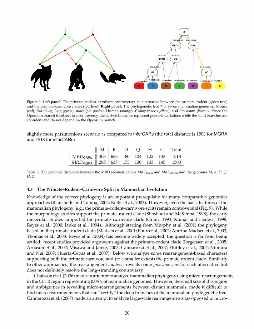
QHC
X
QHC+MROD
MROD
MROD+QHC
HC
HC+MRODQ
Q
Q+MRODHC
H
H+MRODQC
C
C+MRODQH
MR
MRO
MR+ODQHC
D
OD
D+MROQHC
M
M+RODQHC
R
R+MODQHC
O
O+MRDQHC
Figure 9: Left panel: The primate–rodent–carnivore controversy: an alternative between the primate–rodent (green tree)and the primate–carnivore clades (red tree). Right panel: The phylogenetic tree T of seven mammalian genomes: Mouse(red), Rat (blue), Dog (green), macaQue (violet), Human (orange), Chimpanzee (yellow), and Opossum (brown). Since theOpossum branch is subject to a controversy, the dashed branches represent possible variations while the solid branches areconfident and do not depend on the Opossum branch.
slightly more parsimonious scenario as compared to inferCARs (the total distance is 1503 for MGRAand 1518 for inferCARs).
M R D Q H C TotalMRDCARs 303 656 180 124 122 133 1518MRDMGRA 285 637 173 130 133 145 1503
Table 3: The genomic distances between the MRD reconstructions MRDCARs and MRDMGRA and the genomes M, R, D, Q,H, C.
4.3 The Primate–Rodent–Carnivore Split in Mammalian Evolution
Knowledge of the correct phylogeny is an important prerequisite for many comparative genomicsapproaches (Blanchette and Tompa, 2002; Kellis et al., 2003). However, even the basic features of themammalian phylogeny (e.g., the primate–rodent–carnivore split) remain controversial (Fig. 9). Whilethe morphology studies support the primate–rodent clade (Shoshani and McKenna, 1998), the earlymolecular studies supported the primate–carnivore clade (Graur, 1993; Kumar and Hedges, 1998;Reyes et al., 2000; Janke et al., 1994). Although starting from Murphy et al. (2001) the phylogenybased on the primate–rodent clade (Madsen et al., 2001; Poux et al., 2002; Amrine-Madsen et al., 2003;Thomas et al., 2003; Reyes et al., 2004) has become widely accepted, the question is far from beingsettled: recent studies provided arguments against the primate–rodent clade (Jorgensen et al., 2005;Arnason et al., 2002; Misawa and Janke, 2003; Cannarozzi et al., 2007; Huttley et al., 2007; Niimuraand Nei, 2007; Huerta-Cepas et al., 2007). Below we analyze some rearrangement-based characterssupporting both the primate-carnivore and (to a smaller extent) the primate-rodent clade. Similarlyto other approaches, the rearrangement analysis reveals some pros and cons for each alternative butdoes not definitely resolve the long-stranding controversy.
Chaisson et al. (2006) made an attempt to analyze mammalian phylogeny using micro-rearrangementsin the CFTR region representing 0.06% of mammalian genomes. However, the small size of this regionand ambiguities in revealing micro-rearrangements between distant mammals, made it difficult tofind micro-rearrangements that can “certify” the deep branches of the mammalian phylogenetic tree.Cannarozzi et al. (2007) made an attempt to analyze large-scale rearrangements (as opposed to micro-
20

rearrangements) for reconstructing the mammalian evolutionary history. Their approach, whilepromising, left a number of questions unanswered. In particular, Cannarozzi et al. (2007) discussedonly reversals and ignored translocations, fusions, and fissions. Also, they computed the reversaldistances using an (unpublished) greedy algorithm. Since breakpoint re-use is prominent in mam-malian evolution, greedy approaches are unlikely to provide an adequate rearrangement scenario.Finally, Cannarozzi et al. (2007) used the “distance-based” rather than “character-based” methodsfor computing the phylogenetic tree. It is well-known that the performance of the “distance-based”methods deteriorates in the case of large breakpoint re-use typical for mammalian genomes.
Lunter (2007) criticized Cannarozzi et al. (2007) and wrote in April 2007: “It appears unjustified tocontinue to consider the phylogeny of primates, rodents, and canines as contentious”; Huttley et al. (2007)wrote in May 2007: “We have demonstrated with very high confidence that the rodents diverged beforecarnivores and primates” (see Niimura and Nei (2007); Huerta-Cepas et al. (2007) for other recentstudies supporting the primate–carnivore clade). We therefore argue that the rearrangement-basedstudy of the primate–rodent–carnivore controversy is timely.
To analyze the primate–rodent–carnivore controversy, we added the Opossum genome (Mikkelsenet al., 2007) to our rearrangement analysis.12 However, while the phylogenetic tree of the previouslyconsidered six mammalian genomes is well established, the position of the opossum genome in thistree is being debated (Fig. 9). Supplementary Table S13 presents the statistics of the breakpointgraph and reveals simple edges supporting the debated tree topologies. Among the non-confidentbranches, the MRO + DQHC branch (corresponding the primate–carnivore clade) is supported by 50multi-edges, while the DO+MRQHC branch (corresponding to the primate–rodent clade) is supportedby 32 multi-edges. We emphasize that only 4 out of 50 multi-edges supporting the MRO + DQHCbranch represent MRO multi-edges, resulting in a very small number of simple MRO+DQHC vertices(one simple vertex for MRO + DQHC branch as compared to zero simple vertices for DO + MRQHCbranch).
To further address the uncertainty with the opossum branch we applied MGRA only to the non-controversial parts of the tree with the goal to find characters supporting each of two currently debatedtree topologies. The debated tree topologies share (non-controversial) HC + MRDOQ, QHC + MRDO,and MR + DOQHC branches (as well as seven leaf branches corresponding to single genomes). Werefer to these branches as confident and consider only good and fair paths that correspond to confidentbranches in MGRA analysis. To further compare the support for the primate–carnivore and theprimate–rodent clades we run MGRA to simplify this breakpoint graph. MGRA Stages 1-2 result inthe breakpoint graph (Fig. S18(top)) that encodes rearrangements during mammalian radiation.
While running MGRA on all seven genomes was important for simplifying the initial breakpointgraph of seven genomes, it hardly makes sense to analyze all these genomes in the complex graphin Fig. S18(top). Indeed, we are not interested in subtle inconsistencies between mouse–rat andhuman–chimpanzee–macaque genomic architectures revealed by this graph. We therefore selectsingle representatives of the primate (macaque-human-chimpanzee ancestor), rodent (mouse-rat an-cestor), and carnivore (dog) as well as the outgroup (opossum genome) to simplify the analysis (seeFig. S18(top) for a similar analysis with the representatives corresponding to extant macaque, mouse,dog, and opossum genomes).
Table 1(bottom) allows one to analyze features supporting the primate–carnivore clade (26 multi-edges of MO + DQ multicolors) and the primate–rodent (12 multi-edges of MQ + DO multicolors).While the rearrangement-based support for the primate–carnivore clade is more significant than forthe primate–rodent clade (26 versus 12 multi-edges), one cannot exclude a possibility that somecomplex breakpoint re-use events skewed the statistics in Table 1(bottom) in favor of the primate–
12Adding the seventh genome increases the number of the synteny blocks to 1746 (by ≈ 30%) but reduces the coverageof the genomes by the synteny blocks from 89% to 79%.
21

carnivore clade (see Table 4). Since the elephant genome provides a better (less diverged) outgroupthan the opossum genome, there is a hope that the completion of the elephant sequencing projectmay eventually lead to the resolution of the primate-rodent-carnivore controvery.
We re-run MGRA on the set of seven genomes, assuming the primate–carnivore topology.13 Theresulting rearrangement distances as well as 2-breaks assigned to MRO + DQHC branch (supportingthe carnivore-primate split) are given in Supplement H.
Multicolors Multi-edges
Simplevertices
Simplemulti-edges
Simplepaths+cycles
∅ + RPCO 0 + 627 = 627 0 0 + 0 = 0 0 + 0 = 0O + RPC 617 + 740 = 1357 1230 613 + 523 = 1136 93 + 109 = 202R + PCO 280 + 173 = 453 346 121 + 173 = 294 52 + 28 = 80C + RPO 142 + 246 = 388 284 142 + 96 = 238 46 + 33 = 79P + RCO 49 + 124 = 173 98 49 + 31 = 80 18 + 13 = 31RO + PC 5 + 46 = 51 1 0 + 0 = 0 0 + 0 = 0RP + CO 32 + 11 = 43 1 0 + 0 = 0 0 + 0 = 0RC + PO 16 + 8 = 24 2 0 + 0 = 0 0 + 0 = 0
∅ + RPCO 0 + 1712 = 1712 0 0 + 0 = 0 0 + 0 = 0O + RPC 10 + 26 = 36 10 0 + 0 = 0 0 + 0 = 0R + PCO 22 + 5 = 27 5 0 + 0 = 0 0 + 0 = 0C + RPO 0 + 18 = 18 0 0 + 0 = 0 0 + 0 = 0P + RCO 0 + 16 = 16 0 0 + 0 = 0 0 + 0 = 0RO + PC 4 + 16 = 20 6 2 + 1 = 3 2 + 0 = 2RP + CO 5 + 4 = 9 4 0 + 0 = 0 0 + 0 = 0RC + PO 5 + 4 = 9 4 1 + 0 = 1 1 + 0 = 1
∅ + RPCO 0 + 1743 = 1743 0 0 + 0 = 0 0 + 0 = 0O + RPC 0 + 2 = 2 0 0 + 0 = 0 0 + 0 = 0C + RPO 0 + 2 = 2 0 0 + 0 = 0 0 + 0 = 0P + RCO 0 + 1 = 1 0 0 + 0 = 0 0 + 0 = 0RO + PC 9 + 10 = 19 12 3 + 3 = 6 5 + 0 = 5RC + PO 8 + 8 = 16 10 2 + 3 = 5 3 + 1 = 4RP + CO 7 + 8 = 15 10 4 + 2 = 6 4 + 0 = 4
Table 4: The statistics of the breakpoint graph of the ancestral Rodent (mouse-rat ancestor), ancestral Primate (macaque-human-chimpanzee ancestor), Carnivore (dog), and Opossum genomes. The ancestral Rodent and Primate ancestors werereconstructed using MGRA and were used as the genomes in the leaves of the phylogenetic tree for four species: Rodent,Primate, Dog, and Opossum. The statistics is shown for before running MGRA (top table), after MGRA Stage 1 (middletable), and after MGRA Stage 2 (bottom table) run on the leaf branches (i.e., without assuming any particular topology ofthe phylogenetic tree). Compare to Tables 1(bottom) and S13.
DISCUSSION
Recently, Froenicke et al. (2006) expressed a concern about some differences between the rearrangement-based and cytogenetics-based approaches to ancestral genome reconstruction. The problem is thatsome important insights developed by the cytogenetics community still did not find their way into thegenome rearrangement tools like MGR, GRAPPA, inferCARs, and EMRAE. While MGRA started as anattempt to close this gap, we quickly realized that the problem of merging the cytogenetics-based andrearrangement-based approaches is far from being simple. First, there is still no cytogenetics-basedsoftware that can be automatically applied to genome-scale datasets to enable an unbiased compari-son of two approaches on the same dataset. Second, it is not clear how well the cytogenetics approachscales with increase in the resolution, e.g., with 1000+ synteny blocks from Ma et al. (2006).
Despite the low resolution of the cytogenetic data, the cytogenetics-based ancestral reconstructions
13In contrast, Ma et al. (2006) assumed the primate–rodent topology.
22

are very accurate as there are relatively few discrepancies between the cytogenetics-based and therecent genomics-based high-resolution reconstructions (Bourque et al., 2005; Murphy et al., 2005; Maet al., 2006). Moreover, the discrepancies are usually attributed to some arbitrary assignments of thegenomics-based MGR algorithm (Froenicke et al., 2006) rather than errors in the cytogenetics analysis.Indeed, MGR was developed for finding the most parsimonious scenario rather than finding whichrearrangements in this scenario are less reliable than others. The discrepancies between MGR and thecytogenetics-based reconstructions are likely to be a reflection of the “strength in numbers” principlerather than shortcomings of the genomics-based approaches: while the cytogenetic reconstructionsare based on over 100 known cytogenetic maps, there are still only seven completed mammaliangenomic sequences suitable for the rearrangement analysis. However, even with a small increase inthe number of the genomes from 3-4 (as in Bourque et al. (2004, 2005)) to 6-7 (as in Murphy et al.(2005); Ma et al. (2006)), there are very few discrepancies between the cytogenetics-based and thegenomics-based approaches (Rocchi et al., 2006). Despite a recent debate (Froenicke et al., 2006;Bourque et al., 2006), the cytogenetics and genomics-based approaches are converging and benefitingfrom the higher resolution of the genomics-based approaches. However, the key condition for suchconvergence is the availability of algorithms that improve upon the existing heuristics for separatingbetween strong and weak associations. We addressed this challenge by devising MGRA algorithmthat remedies some limitations of the previous approaches to ancestral reconstructions. Similarlyto the algoritms recently proposed by Ma et al. (2008); Chauve and Tannier (2008) (published afterthis paper was submitted), MGRA focuses on accurate rather than the most parsimonious ancestralreconstructions.
ACKNOWLEDGEMENTS
We are indebted to Jian Ma for providing us with the synteny blocks for mammalian genomesfrom the latest builds and for numerous thoughtful discussions. We are thankful to Bill Murphy fora discussion about the primate–rodent–carnivore controversy as well as to Guillaume Bourque andGlenn Tesler for discussions on the algorithmic aspects of this project. We are also grateful to LutzFroenicke and Claus Kemkemer for useful comments on the cytogenetics approach and CytoAncestor.This work was supported by the Howard Hughes Professor Award.
23

ReferencesAlekseyev, M. A., 2008. Multi-Break Rearrangements and Breakpoint Re-uses: from Circular to Linear Genomes. Journal of
Computational Biology, 15(8):1117–1131.
Alekseyev, M. A. and Pevzner, P. A., 2007. Whole Genome Duplications, Multi-Break Rearrangements, and Genome HalvingTheorem. Proceedings of the 18th Annual ACM-SIAM Symposium on Discrete Algorithms (SODA), :665–679.
Alekseyev, M. A. and Pevzner, P. A., 2008. Multi-Break Rearrangements and Chromosomal Evolution. Theoretical ComputerScience, 395(2-3):193–202.
Amrine-Madsen, H., Koepfli, K.-P., Wayne, R. K., and Springer, M. S., 2003. A new phylogenetic marker, apolipoprotein B,provides compelling evidence for eutherian relationships. Molecular Phylogenetics and Evolution, 28(2):225–240.
Arnason, U., Adegoke, J. A., Bodin, K., Born, E. W., Esa, Y. B., Gullberg, A., Nilsson, M., Short, R. V., Xu, X., and Janke, A.,et al., 2002. Mammalian mitogenomic relationships and the root of the eutherian tree. Proceedings of the National Academyof Sciences, 99(12):8151–8156.
Bafna, V. and Pevzner, P. A., 1996. Genome rearrangement and sorting by reversals. SIAM Journal on Computing, 25:272–289.
Bafna, V. and Pevzner, P. A., 1998. Sorting permutations by transpositions. SIAM J. Discrete Math., 11:224–240.
Bailey, J., Baertsch, R., Kent, W., Haussler, D., and Eichler, E., 2004. Hotspots of mammalian chromosomal evolution. GenomeBiology, 5(4):R23.
Bergeron, A., Mixtacki, J., and Stoye, J., 2006. A Unifying View of Genome Rearrangements. Lecture Notes in ComputerScience, 4175:163–173.
Blanchette, M., Bourque, G., and Sankoff, D., 1997. Breakpoint Phylogenies. Genome Informatics, 8:25–34.
Blanchette, M. and Tompa, M., 2002. Discovery of Regulatory Elements by a Computational Method for PhylogeneticFootprinting. Genome Research, 12(5):739–748.
Bourque, G. and Pevzner, P. A., 2002. Genome-Scale Evolution: Reconstructing Gene Orders in the Ancestral Species.Genome Research, 12(1):26–36.
Bourque, G., Pevzner, P. A., and Tesler, G., 2004. Reconstructing the genomic architecture of ancestral mammals: lessonsfrom human, mouse, and rat genomes. Genome Research, 14:507–516.
Bourque, G., Tesler, G., and Pevzner, P. A., 2006. The convergence of cytogenetics and rearrangement-based models forancestral genome reconstruction. Genome Res., 16(3):311–313.
Bourque, G., Zdobnov, E. M., Bork, P., Pevzner, P. A., and Tesler, G., 2005. Comparative architectures of mammalian andchicken genomes reveal highly variable rates of genomic rearrangements across different lineages. Genome Research,15:98–110.
Bulazel, K., Ferreri, G., Eldridge, M., and O’Neill, R., 2007. Species-specific shifts in centromere sequence composition arecoincident with breakpoint reuse in karyotypically divergent lineages. Genome Biology, 8(8):R170.
Caceres, M., Sullivan, R. T., and Thomas, J. W., 2007. A recurrent inversion on the eutherian X chromosome. Proceedings ofthe National Academy of Sciences, 104(47):18571–18576.
Cannarozzi, G., Schneider, A., and Gonnet, G., 2007. A Phylogenomic Study of Human, Dog, and Mouse. PLoS ComputationalBiology, 3(1):e2.
Caprara, A., 1999a. Formulations and hardness of multiple sorting by reversals. In RECOMB ’99: Proceedings of the thirdannual international conference on Computational molecular biology, pages 84–93, New York, NY, USA. ACM.
Caprara, A., 1999b. On the Tightness of the Alternating-Cycle Lower Bound for Sorting by Reversals. Journal of CombinatorialOptimization, 3(2-3):149–182.
Cardone, M., Jiang, Z., D’Addabbo, P., Archidiacono, N., Rocchi, M., Eichler, E., and Ventura, M., 2008. Hominoidchromosomal rearrangements on 17q map to complex regions of segmental duplication. Genome Biology, 9(2):R28.
24

Chaisson, M. J., Raphael, B. J., and Pevzner, P. A., 2006. Microinversions in mammalian evolution. Proceedings of the NationalAcademy of Sciences, 103(52):19824–19829.
Chauve, C. and Tannier, E., 2008. A Methodological Framework for the Reconstruction of Contiguous Regions of AncestralGenomes and Its Application to Mammalian Genomes. PLoS Computational Biology, 4(11):e1000234.
Deuve, J., Bennett, N., Britton-Davidian, J., and Robinson, T., 2008. Chromosomal phylogeny and evolution of the africanmole-rats (bathyergidae). Chromosome Research, 16(1):57–74.
Feuk, L., MacDonald, J. R., Tang, T., Carson, A. R., Li, M., Rao, G., Khaja, R., and Scherer, S. W., 2005. Discovery ofHuman Inversion Polymorphisms by Comparative Analysis of Human and Chimpanzee DNA Sequence Assemblies.PLoS Genetics, 1:e56.
Froenicke, 2005. Origins of primate chromosomes – as delineated by zoo-fish and alignments of human and mouse draftgenome sequences. Cytogenetic and Genome Research, 108(1-3):122–138.
Froenicke, L., Caldes, M. G., Graphodatsky, A., Muller, S., Lyons, L. A., Robinson, T. J., Volleth, M., Yang, F., and Wienberg,J., 2006. Are molecular cytogenetics and bioinformatics suggesting diverging models of ancestral mammalian genomes?Genome Res., 16(3):306–310.
Gordon, L., Yang, S., Tran-Gyamfi, M., Baggott, D., Christensen, M., Hamilton, A., Crooijmans, R., Groenen, M., Lucas, S.,Ovcharenko, I., et al., 2007. Comparative analysis of chicken chromosome 28 provides new clues to the evolutionaryfragility of gene-rich vertebrate regions. Genome Research, 17(11):1603–1613.
Graur, D., 1993. Towards a molecular resolution of the ordinal phylogeny of the eutherian mammals. FEBS Letters,325(1-2):152–159.
Hannenhalli, S. and Pevzner, P., 1995. Transforming men into mouse (polynomial algorithm for genomic distance problem).Proceedings of the 36th Annual Symposium on Foundations of Computer Science, :581–592.
Hannenhalli, S. and Pevzner, P., 1999. Transforming cabbage into turnip (polynomial algorithm for sorting signed permu-tations by reversals). Journal of the ACM, 46:1–27.
Hinsch, H. and Hannenhalli, S., 2006. Recurring genomic breaks in independent lineages support genomic fragility. BMCEvolutionary Biology, 6:90.
Huerta-Cepas, J., Dopazo, H., Dopazo, J., and Gabaldon, T., 2007. The human phylome. Genome Biology, 8(6):R109.
Huttley, G. A., Wakefield, M. J., and Easteal, S., 2007. Rates of Genome Evolution and Branching Order from Whole GenomeAnalysis. Molecular Biology and Evolution, 24(8):1722–1730.
Janke, A., Feldmaier-Fuchs, G., Thomas, W. K., von Haeseler, A., and Paabo, S., 1994. The Marsupial Mitochondrial Genomeand the Evolution of Placental Mammals. Genetics, 137(1):243–256.
Jorgensen, F., Hobolth, A., Hornshoj, H., Bendixen, C., Fredholm, M., and Schierup, M., 2005. Comparative analysis ofprotein coding sequences from human, mouse and the domesticated pig. BMC Biology, 3(1):2.
Kellis, M., Patterson, N., Endrizzi, M., Birren, B., and Lander, E. S., 2003. Sequencing and comparison of yeast species toidentify genes and regulatory elements. Nature, 423(6937):241–254.
Kemkemer, C., Kohn, M., Kehrer-Sawatzki, H., Minich, P., Hogel, J., Froenicke, L., and Hameister, H., 2006. Reconstructionof the ancestral ferungulate karyotype by electronic chromosome painting (E-painting). Chromosome Research, 14(8):899–907.
Kikuta, H., Laplante, M., Navratilova, P., Komisarczuk, A. Z., Engstrom, P. G., Fredman, D., Akalin, A., Caccamo, M., Sealy,I., Howe, K., et al., 2007. Genomic regulatory blocks encompass multiple neighboring genes and maintain conservedsynteny in vertebrates. Genome Research, 17(5):545–555.
Kumar, S. and Hedges, S. B., 1998. A molecular timescale for vertebrate evolution. Nature, 392(6679):917–920.
Lin, Y. and Moret, B. M., 2008. Estimating true evolutionary distances under the DCJ model. Bioinformatics, 24(13):i114–122.
Lunter, G., 2007. Dog as an Outgroup to Human and Mouse. PLoS Computational Biology, 3(4):e74.
25

Ma, J., Ratan, A., Raney, B. J., Suh, B. B., Miller, W., and Haussler, D., 2008. The infinite sites model of genome evolution.Proceedings of the National Academy of Sciences, 105(38):14254–14261.
Ma, J., Zhang, L., Suh, B. B., Raney, B. J., Burhans, R. C., Kent, J. W., Blanchette, M., Haussler, D., and Miller, W., 2006.Reconstructing contiguous regions of an ancestral genome. Genome Research, 16(12):1557–1565.
Madsen, O., Scally, M., Douady, C. J., Kao, D. J., DeBry, R. W., Adkins, R., Amrine, H. M., Stanhope, M. J., de Jong,W. W., and Springer, M. S., et al., 2001. Parallel adaptive radiations in two major clades of placental mammals. Nature,409(6820):610–614.
Mehan, M. R., Almonte, M., Slaten, E., Freimer, N. B., Rao, P. N., and Ophoff, R. A., 2007. Analysis of segmental duplicationsreveals a distinct pattern of continuation-of-synteny between human and mouse genomes. Human Genetics, 121(1):93–100.
Mikkelsen, T. S., Wakefield, M. J., Aken, B., Amemiya, C. T., Chang, J. L., Duke, S., Garber, M., Gentles, A. J., Goodstadt, L.,Heger, A., et al., 2007. Genome of the marsupial monodelphis domestica reveals innovation in non-coding sequences.Nature, 447(7141):167–177.
Misawa, K. and Janke, A., 2003. Revisiting the Glires concept–phylogenetic analysis of nuclear sequences. MolecularPhylogenetics and Evolution, 28(2):320–327.
Moret, B., Wyman, S., Bader, D. A., Warnow, T., and Yan, M., 2001. A new implementation and detailed study of breakpointanalysis. Pacific Symposium on Biocomputing, :583–594.
Moret, B. M. E., Siepel, A. C., Tang, J., and Liu, T., 2002. Inversion Medians Outperform Breakpoint Medians in PhylogenyReconstruction from Gene-Order Data. Lecture Notes In Computer Science, 2452:521–536.
Murphy, W. J., Eizirik, E., Johnson, W. E., Zhang, Y. P., Ryder, O. A., and O’Brien, S. J., 2001. Molecular phylogenetics andthe origins of placental mammals. Nature, 409(6820):614–618.
Murphy, W. J., Larkin, D. M., van der Wind, A. E., Bourque, G., Tesler, G., Auvil, L., Beever, J. E., Chowdhary, B. P., Galibert,F., Gatzke, L., et al., 2005. Dynamics of Mammalian Chromosome Evolution Inferred from Multispecies ComparativeMap. Science, 309(5734):613–617.
Niimura, Y. and Nei, M., 2007. Extensive Gains and Losses of Olfactory Receptor Genes in Mammalian Evolution. PLoSONE, 2(8):e708.
Ozery-Flato, M. and Shamir, R., 2003. Two Notes on Genome Rearrangement. Journal of Bioinformatics and ComputationalBiology, 1:71–94.
Pevzner, P. A., 2000. Computational Molecular Biology: An Algorithmic Approach. The MIT Press, Cambridge.
Pevzner, P. A. and Tesler, G., 2003. Human and mouse genomic sequences reveal extensive breakpoint reuse in mammalianevolution. Proceedings of the National Academy of Sciences, 100:7672–7677.
Pontius, J. U., Mullikin, J. C., Smith, D. R., Lindblad-Toh, K., Gnerre, S., Clamp, M., Chang, J., Stephens, R., Neelam, B.,Volfovsky, N., et al., 2007. Initial sequence and comparative analysis of the cat genome. Genome Research, 17(11):1675–1689.
Poux, C., van Rheede, T., Madsen, O., and de Jong, W. W., 2002. Sequence Gaps Join Mice and Men: Phylogenetic Evidencefrom Deletions in Two Proteins. Mol Biol Evol, 19(11):2035–2037.
Reyes, A., Gissi, C., Catzeflis, F., Nevo, E., Pesole, G., and Saccone, C., 2004. Congruent Mammalian Trees from Mitochondrialand Nuclear Genes Using Bayesian Methods. Molecular Biology and Evolution, 21(2):397–403.
Reyes, A., Gissi, C., Pesole, G., Catzeflis, F. M., and Saccone, C., 2000. Where Do Rodents Fit? Evidence from the CompleteMitochondrial Genome of Sciurus vulgaris. Mol Biol Evol, 17(6):979–983.
Robinson, T. J., Ruiz-Herrera, A., and Froenicke, L., 2006. Dissecting the mammalian genome – new insights into chromo-somal evolution. Trends in Genetics, 22(6):297–301.
Rocchi, M., Archidiacono, N., and Stanyon, R., 2006. Ancestral genomes reconstruction: An integrated, multi-disciplinaryapproach is needed. Genome Res., 16(12):1441–1444.
Ruiz-Herrera, A., Castresana, J., and Robinson, T. J., 2006. Is mammalian chromosomal evolution driven by regions ofgenome fragility? Genome Biology, 7:R115.
26

Sankoff, D. and Blanchette, M., 1998. Multiple genome rearrangement and breakpoint phylogeny. Journal of ComputationalBiology, 5(3):555–570.
Sankoff, D., Leduc, G., Antoine, N., Paquin, B., Lang, B. F., and Cedergren, R., 1992. Gene Order Comparisons for Phyloge-netic Inference: Evolution of the Mitochondrial Genome. Proceedings of the National Academy of Sciences, 89(14):6575–6579.
Shoshani, J. and McKenna, M. C., 1998. Higher Taxonomic Relationships among Extant Mammals Based on Morphology,with Selected Comparisons of Results from Molecular Data. Molecular Phylogenetics and Evolution, 9(3):572–584.
Tang, J. and Moret, B. M., 2003. Scaling up accurate phylogenetic reconstruction from gene-order data. Bioinformatics,19(Suppl. 1):i305–312.
Tannier, E. and Sagot, M.-F., 2004. Sorting by reversals in subquadratic time. Lecture Notes in Computer Science, 3109:1–13.
Tannier, E., Zheng, C., and Sankoff, D., 2008. Multichromosomal Genome Median and Halving Problems. Lecture Notes inBioinformatics, 5251:1–13.
Tesler, G., 2002a. Efficient algorithms for multichromosomal genome rearrangements. J. Comput. Syst. Sci., 65:587–609.
Tesler, G., 2002b. GRIMM: genome rearrangements web server . Bioinformatics, 18(3):492–493.
Thomas, J. W., Touchman, J. W., Blakesley, R. W., Bouffard, G. G., Beckstrom-Sternberg, S. M., Margulies, E. H., Blanchette,M., Siepel, A. C., Thomas, P. J., McDowell, J. C., et al., 2003. Comparative analyses of multi-species sequences fromtargeted genomic regions. Nature, 424(6950):788–793.
van der Wind, A. E., Kata, S. R., Band, M. R., Rebeiz, M., Larkin, D. M., Everts, R. E., Green, C. A., Liu, L., Natarajan,S., Goldammer, T., et al., 2004. A 1463 Gene Cattle-Human Comparative Map With Anchor Points Defined by HumanGenome Sequence Coordinates. Genome Research, 14(7):1424–1437.
Webber, C. and Ponting, C. P., 2005. Hotspots of mutation and breakage in dog and human chromosomes. Genome Research,15(12):1787–1797.
Wienberg, J. and Stanyon, R., 1997. Comparative painting of mammalian chromosomes. Current Opinion in Genetics &Development, 7(6):784–791.
Xia, A., Sharakhova, M., and Sharakhov, I., 2007. Reconstructing an inversion history in the anopheles gambiae complex.Lecture Notes in Bioinformatics, 4751:136–148.
Yancopoulos, S., Attie, O., and Friedberg, R., 2005. Efficient sorting of genomic permutations by translocation, inversionand block interchange. Bioinformatics, 21:3340–3346.
Yue, Y. and Haaf, T., 2006. 7E olfactory receptor gene clusters and evolutionary chromosome rearrangements. Cytogeneticand Genome Research, 112:6–10.
Zhao, H. and Bourque, G., 2007. Recovering True Rearrangement Events on Phylogenetic Trees. Lecture Notes in Bioinfor-matics, 4751:149–161.
Zhao, S., Shetty, J., Hou, L., Delcher, A., Zhu, B., Osoegawa, K., de Jong, P., Nierman, W. C., Strausberg, R. L., and Fraser,C. M., et al., 2004. Human, Mouse, and Rat Genome Large-Scale Rearrangements: Stability Versus Speciation. GenomeResearch, 14:1851–1860.
27

Supplement A Independent, semi-independent, and weakly-independent rearrange-ments
Let P be a genome represented a graph on black and obverse edges. For any m black edges in P, wedefine an m-break (or multi-break) rearrangement as replacement of these edges with other m blackedges forming a matching on the same vertices (see Alekseyev and Pevzner (2008); Alekseyev (2008)).
Let P1,P2, . . . ,Pk be genomes that evolved by some unknown multi-breaks following an unknownevolutionary tree (we allow any combination of 2-breaks, 3-breaks, and m-breaks for m > 3 in a singleevolutionary scenario). Without loss of generality, we assume that there was at least one multi-breakon every branch of the tree. One may classify an m-break as independent if it does not reuse breakpoints,i.e., creates exactly m new breakpoints. Similarly, we call the rearrangement scenario independent ifall its multi-breaks are independent.
If all multi-breaks are independent, the following theorem applies (the proof follows the proof ofa similar result in Chaisson et al. (2006)).
Theorem 1. If genomes P1,P2, . . . ,Pk are produced by independent multi-breaks, then both the correct evolu-tionary tree for these genomes and the ancestral genomes in all its branching nodes may be reconstructed inpolynomial time.
We now consider the case when genomes P1,P2, . . . ,Pk are produced by semi-independent 2-breaksthat may re-use breakpoints within single branches of the evolutionary tree (i.e., a semi-independent2-break does not share breakpoints with any other 2-break on a different branch of T). We callthe 2-break rearrangement scenario semi-independent if all its 2-breaks are semi-independent. Sinceany semi-independent 2-break scenario corresponds to an independent multi-break scenario (seeAlekseyev and Pevzner (2008)), Theorem 1 implies:
Theorem 2. If genomes P1,P2, . . . ,Pk are produced by semi-independent 2-breaks, then both the correctevolutionary tree for these genomes and the ancestral genomes in all its branching nodes may be reconstructedin polynomial time.
MGRA optimally solves the MGRP problem in case of semi-independent 2-breaks and uses heuris-tics to move beyond the semi-independent assumption. In a new manuscript14 we define the notion ofweakly independent rearrangements that relaxes the semi-independent assumption by allowing break-point re-uses within selected pairs of incident branches in the phylogenetic tree (as opposed to a singlebranch in semi-independent scenarios). We demonstrate that the TCMGRP can be solved efficientlyin the case of weakly independent scenarios.15 Below we show that most 2-breaks in mammalianevolution are either independent, or semi-independent, or weakly independent resulting in reliableancestral reconstructions. The theoretical analysis of weakly independent scenarios is not crucial forunderstanding MGRA and will be described elsewhere.
Supplement B Simultaneous T-consistent transformationsThe problem of finding a shortest rearrangement scenario typically has many solutions. To character-ize all genomes that may appear in shortest rearrangement scenarios between genomes A and B, wesay that a genome Q is located between A and B if the rearrangement distances between these genomessatisfy the condition: d(A,Q) + d(Q,B) = d(A,B). In the case of a phylogenetic tree T with knowngenomes at all internal nodes, we say that a genome Q is located on a branch (A,B) of the phylogenetictree T if it located between nodes (genomes) A and B. Similarly, a genome Q is located on the tree T ifit is located on a branch of T. A transformation between two genomes located on the tree T is calledT-consistent if every intermediate genome in this transformation is also located on T.
14M. Alekseyev and P. Pevzner. “Breakpoint Re-uses and Efficient Ancestral Genome Reconstruction”. Mimeo.15In particular, while the reversal median problem is NP-complete for arbitrary scenarios (Caprara, 1999a), one can
efficiently reconstruct the 2-break median for 3 genomes in case of weakly independent scenarios.
28

Let T be a tree with known genomes specified at every node. A tree T′ is homeomorphic to thetree T if it is derived from T by adding extra internal nodes (of degree 2) within branches of T andspecifying some genomes at these added nodes. For example, Fig. 3c represents a tree homeomorphicto the tree in Fig. 3a with two extra nodes added to the branch (Q2,Q3). A homeomorphic tree T′
defines a T-consistent rearrangement scenario if genomes at every two adjacent nodes of T′ differ fromeach other by a single rearrangement and the total number of rearrangements along each branch isminimal. We now reformulate the problem of finding the most parsimonious rearrangement scenarioas the problem of finding a T-consistent rearrangement scenario with the minimum number of nodesin the homeomorphic tree T′.
If X is an arbitrary genome (root) in T′ then the path path(X,Pi) from the root X to every leafgenome Pi in T′ corresponds to a series of rearrangements transforming X into Pi (i = 1, 2, . . . , k). A setof nodes C in T′ is called a cut if each path path(X,Pi) contains exactly one node from C (for 1 ≤ i ≤ k).For example, the sets {X} and {P1, . . . ,Pk} represent cuts in T′ with minimum and maximum numberof nodes correspondingly. Given a cut C and a leaf genome Pi, let vC
i be a (single) node in C locatedon a path path(X,Pi) and let PC
i be the genome assigned to the node vCi . Therefore, every cut C defines
k genomes PCi1 ,P
Ci2 , . . .P
Cik .
One can orient branches of T′ in the direction from X to the leaves and define next(v) as the setof children of an internal node v (the number of children equals the degree of v minus one). Givenan internal node v in a cut C, we define a new cut nextv(C) obtained from C by deleting a node v andadding the set of nodes next(v). A simultaneous T-consistent transformation of the root genome X into theleaf genomes P1, . . . ,Pk is a series of cuts {X} = C0,C1, . . . ,Cd = {P1, . . . ,Pk} such that Ci+1 = nextvi(Ci)for some node vi ∈ Ci (0 ≤ i < d). It is easy to see that for every T-consistent transformationthere exists a simultaneous T-consistent transformation. Below we give an equivalent definition ofthe simultaneous T-consistent transformation in terms of multiple breakpoint graphs that motivatesMGRA algorithm attempting to find a shortest simultaneous T-consistent transformation.
Any subset of edges from the multi-edge (x, y) represents a sub-multi-edge (x, y) of the multi-color formed by the colors of the edges in this subset. Any simultaneous T-consistent transfor-mation of X into P1, . . . ,Pk defines a transformation of the identity breakpoint graph G(X, . . . ,X)into G(P1,P2, . . . ,Pk) with a series of rearrangements applied to sub-multi-edges of T-consistentmulticolors. Namely, we define the multiple breakpoint graph corresponding to the cut Ci asGi = G(PCi
1 ,PCi2 , . . . ,P
Cik ). It is easy to see that Gi+1 is obtained from Gi by a single rearrangement
ρ applied to all copies of some genome Q in PCi1 ,P
Ci2 , . . . ,P
Cik . Alternatively, a transformation of
Gi into Gi+1 can be viewed as applying ρ to T-consistent sub-multi-edges in Gi (of the multicolor{Pi | PCi = Q}).
Supplement C Reconstructing reliable CARsTo reconstruct reliable adjacencies in the ancestor genome at a node of the phylogenetic tree, weselect this node as a root node X. Then we start to eliminate breakpoints in the breakpoint graphG(P1, . . . ,Pk) with reliable 2-breaks (for whatever definition of reliability) and stop when no furtherreliable 2-breaks exist. In the resulting breakpoint graph (that may still have some breakpoints) themulti-edges of multicolors containing X (as a subset of colors) represent the reliable block adjacenciesin the target ancestor genome, and we generate CARs based only on such adjacencies. Note thatthis approach can reconstruct CARs in only one ancestor genome at a time, and multiple runs (withdifferent root nodes X) are needed to reconstruct CARs in multiple ancestor genomes.
Supplement D Comparison of various ancestral reconstructions for a component of thebreakpoint graph representing the human chromosomes 7, 16, and 19
Below we focus on the connected component of the breakpoint graph representing the human chro-mosomes 7, 16, and 19 where the cytogenetics approach disagrees with Ma et al. (2006). The advantage
29

of the breakpoint graph approach is that it enables a simple analysis of this controversy since the anal-ysis is reduced to “genomes” with only 6 synteny blocks after equivalent transformations performedby MGRA Stage 1 (Fig. S13). Indeed, the genomes represented by this component can now be viewedas:
Macaque: 4, 5, (2,−6), (3,−1)Mouse: 2, 3, (4, 6), (1,−5)Dog: 1, (4,−6,−5), (2,−3)
where the block 1 is located on the human chromosome 7, the blocks 2 and 3 are located on thehuman chromosome 16 and the blocks 4, 5, 6 are located on the human chromosome 19 (Fig. S11,top panel and Fig. S13). Ma et al. (2006) proposed the ancestral architecture with 4 chromosomes1, 5, (2,−3), (6,−4) (no associations between chromosomes 7, 16, and 19), while Froenicke et al. (2006)proposed 4, 5, (1,−3), (2,−6) (associations 16 + 7 and 16 + 19). It is easy to see that the cytogeneticsreconstruction is less parsimonious than Ma et al. (2006) reconstruction. We therefore argue that thecriticism of Ma et al. (2006) in Rocchi et al. (2006) regarding the missing association 7 + 16 is not fullyjustified since the whole genome data do not support this associations.16
MGRA Stage 2 also generates a solution that improves on the cytogenetics reconstruction (Froenickeet al., 2006) and proposes the ancestral association 7 + 19. While both our and Ma et al. (2006) so-lutions are more parsimonious than the cytogenetics reconstruction, we are not claiming that thesesolutions are necessarily correct (the most parsimonious scenarios on 6 genomes are not necessarilythe most parsimonious scenarios on 100+ genomes). The important thing is that MGRA Stage 1reduces analysis of the 7/16/19 controversy to such a small example that all possible scenarios can beexplored.
Supplement E Selecting fair multi-edges in MGRA Stage 2As described in the main text, the order of selected fair multi-edges may affect the ancestral recon-structions at some nodes of the phylogenetic tree. Below we specify how MGRA Stage 2 selects suchedges.
Note that if a fair multi-edge is not ~T-consistent then this multi-edge can only be affected by 2-breaks on adjacent multi-edges. Although two such 2-breaks are possible, ordering of these 2-breaksdoes not influence the final result (see Fig. 6, bottom panel). However, the situations when two fairmulti-edges share a vertex (and both are ~T-consistent) may be ambiguous since the final result of theirprocessing may be affected by the order in which these edges are processed. MGRA Stage 2 starts byprocessing unambiguous fair edges first and selects the order of remaining fair edges according tothe following heuristics.
For a fixed ~T-consistent multicolor Q, an “ideal” 2-break of multicolor Q should satisfy twoconditions: (i) it increases the number of cycles alternating between every pair of colors from Q + Q(i.e., one color from Q while the other is from Q), and (ii) it does not decrease the number of cyclesalternating between the other pairs of colors. It is easy to see that if a 2-break on a ~T-consistentmulticolor Q increases the number of connected components in the breakpoint graph then both theseconditions are satisfied. For each ~T-consistent multicolor Q, MGRA Stage 2 finds all 2-breaks onmulticolor Q that increase the number of connected components and perform them (in an arbitraryorder).
Supplement F MGRA Stage 3: Processing complex breakpointsIf one attempts to find the positions and orientations of short synteny block in the ancestors, thereare two possibilities. If the signs of the blocks are inferred correctly then the same micro-inversion
16We are not claiming that the analysis of 7 + 16 association in Froenicke (2005); Robinson et al. (2006) is incorrect butinstead argue that it is not supported by data used in Ma et al. (2006).
30

1000h
1001t
1000t
999h
1001h
1002t
1002h
1034h
1003h
1035t
1003t
1004t
1004h
1005t
1005h
1006t
1006h
1007t
1007h
1008t
1008h
1009t
1009h1010t
100h
101t
100t
99h
1010h
1011t
1011h
1012t
1012h
1013t
1013h
1014h
1014t
1017h
1015h
1016t
1015t
1018t
1016h
1017t
1018h
1019t
1019h
1020h
101h
102t
1020t
1027t
1021h
1022t
1021t
1030t
1022h
1023t
1023h
1024t
1024h
1025t
1025h
1026t
1026h
1029h
1027h
1028t
1028h
1029t
102h
103t
1030h
1031t
1031h
1032t
1032h
1033h
1033t
1034t
1035h
970h
1036h
1037t
1036t
1037h
1038t
1038h 1039t
1039h
1040t
103h
104t
1040h
1041t
1041h
1042t
1042h
1043t
1043h
1045h
1044h
1049h
1044t
1048h
1045t
1046t
1046h
1047t
1047h
1048t
1049t
1050t
104h105t
1050h
1051h
1051t
1052t
1052h
1053t
1053h
1055t
1054h
1056t
1054t
1055h
1056h
1059h
1057h
1058t
1057t
1059t
1058h
1060h
105h 106t
1060t
1061t
1061h
1062t 555t
1062h
1063t
1191h
1063h
1064t
1064h
1065t
1065h
1066t
1066h
1067t
1067h
1068t
1068h
1069t
1069h
1070t
106h
107t
1070h
1071t
1071h
1072t
1072h
1073h
1073t
1074t
1074h
1075t
1075h
1076t
1076h
1077t
1077h
1078t
1078h1079t
1079h1080t
107h
108t
1080h1081t
1081h
1082h
1083t
1082t
1103h
1083h
1084t
1084h
1085t
1085h
1086t
1086h
1087t
1087h1088h
1088t
1089t
1089h
1090t
108h
109t
1090h
1091t
1091h
1092t
1092h
1093t
1093h
1095h
1094h
1095t
1094t
1096t
1096h
1097t
1097h
1098h
1099t
1098t
1105t
1099h
1100t
109h
110t
10h
11t
10t
9h
1100h
1101t
1101h
1102t
1102h
1103t
1104h
1106t
1104t
1105h
1106h
1116t
1107h
1108t
1107t
1120t
1108h
1109t
1109h
1110t
110h
111t
1110h
1111t
1111h
1112t
1112h
1114h
1113h
1115t
1113t
1114t
1115h
1121t
1116h
1117t
1117h
1118t
1118h
1119t
1119h
1120h
111h
112t
1121h
1122t
1122h
1123t
1123h
1124t
1124h
1125t
1125h
1126t
1126h
1127t
1127h
1128t
1128h
1129t
1129h
112h
113t
1130h1131t
1130t
1143t
1131h
1132t
1132h
1133h
1133t
1134t
1134h
1135t
1135h
1136t
1136h
1137t
1137h
1138t
1138h
1139t
1139h1140t
113h
114t
1140h
1141t
1141h
1142t
1142h
1143h
1144t
1144h
1145t
1145h
1146t
1146h
1147t
1147h
1148t
1148h
1149t
1149h
1150t
114h115t
1150h
1151t
1151h
1152t
1152h
1153t
1153h
1154t
1154h
1155t
1155h
1156t
1156h
1157t
1157h
1158t
1158h
1159t
1159h
1160t
115h
116t
1160h
1161t
1161h
1162t
1162h
1163t
1163h
1164t
1164h
1165t
1165h
1166t
1166h
1167t
1167h
1168t
1168h
1169t
1169h
1170t
116h
117t
1170h
1171t
1171h
1172t
1172h
1173h
1174t
1173t
1174h
1175t
1175h1176t
1176h
1177t
1177h
1180h
1178h
1179t
1178t1181t
1179h
1180t
117h118t
1181h
1182t
1182h
1183t
1183h1184t
1184h
1185t
1185h
1186t
1186h
1187t
1187h
1188t
1188h
1189t
1189h
1190t
118h
119t
1190h
1191t
1192t
1192h
1193t
1193h
1194t
1194h
1195t
1195h
1196t
1196h
1198h
1197h
1198t
1197t
1199h
1199t
1201h
1200t
1204t
1202t
119h
120t
11h
12t
1200h
1201t
1203h
1202h
1203t
1204h
1205t
1205h
1206t
1206h
1207t
1207h
1208t
1208h
1209t
1209h
1210t
120h
1210h
1211t
1211h
1212t
1212h
1213t
1213h
1214t
1214h
1215t
1215h
1216t
1216h
1217t
1217h
1218t
1218h
1219t
1219h
121h
122t 121t
128t
1220h
1221t
1220t
1225t
1221h
1222t
1222h
1223t
1223h
1224t
1224h1239t
250t
71h
1225h
1226t
1226h
1227t
1227h
1228t
1228h
1229t
1229h
1230t
122h
123t
1230h
1231h
1232t
1231t
216t
1232h
1233t
1233h
1234t
1234h
1235t
1235h
1236t
1236h
1237t
1237h
1238t
1238h
1239h
1241h
123h
124t
1240h
1241t
1240t
1242t
1242h
1243h
1243t
1244h
1244t
1245t
1245h
1246h
1246t
1247h
1248t
1247t
917t
1248h
1249t
1249h
1250t
124h
125t
1250h
1251t
1251h
1252t
1252h
1253t
1253h
1254t
1254h
1255h
1256t
1255t
916h
1256h
1257t
1257h
1258t
1258h
1259t
1259h
1260t
125h
126t
1260h
1261t
1261h
1262t
1262h
1263h
1263t
1264t
1264h667t
76h
1265h
1266t
1265t
1266h
1267t
1267h
1269t
1269h
1270t
126h
127t
1270h
1271t
1271h
1272t
1272h
1273h
1273t
1274t
1274h
1275t
1275h
1276t
1276h
1277t
1277h
1278t
1278h
1279t
1279h1280t
127h
1280h
1281t
1281h
1282t
1282h
1283t
1283h
1284t1284h
1285t
1285h
1286t
1286h
1287t
1287h
1288t1288h
1289t
1289h
1290t
128h
129t
1290h 1291t 1291h1292h
1292t 1293t1293h 1294t
1294h
1295t
1295h
1296t
1296h
1297t
1297h1298t
1298h
1299t
1299h1300t
129h
130t
12h
13t
1300h
1301t
1301h
1302t
1302h 1303t
1303h
1304t
1304h
1305t
1305h
1306t
1306h
1307t
1307h 1308t1308h
1309t
1309h
1310t
130h
131t
1310h
1311t
1311h
1312t
1312h
1313t
1313h
1314t
1314h
1315t
1315h
1316t
1316h
1317t
1317h
1318t
1318h
1319t
1319h
1320t
131h
1320h
1321t
1321h
1322t
1322h
1323t
1323h1324t
1324h
1325t
1325h
1326t
1326h
1327t
1327h
1328t
1328h
1329t
1329h
1330t
132h
133t
132t
143t
1330h
1331t
1331h
1332t
1332h
1333t
1333h
1334t
1334h
1335t
1335h
1336t
1336h
1337t
1337h1339h
1338h
1339t
1338t
1340t
133h
134t
1340h
1341t
1341h1342t1342h
1343t
1343h
1344t1344h
1345t
1345h1346t
1346h
1347t1347h
1348t
1348h1349t
1349h
1350t
134h
135t
1350h
1351t
1351h
1352t
1352h1354t
1354h
1355t
1355h1356t
1356h
1357t
1357h1358t
1358h
1359t
1359h
135h
136t
136h
137t
137h
138t138h
139t
139h
140t
13h
14t
140h
141t
141h
142h
142t
143h
144t144h
145t
145h
146t146h
147t
147h148t
148h
149t
149h
150t
14h
15t
150h
151t
151h
152t
152h153t
153h154t
154h
155t
155h
156t
156h157h157t
158t
158h
159t
159h
160t
15h
16t
160h
161t
161h
162t
162h
163t
163h
164t
164h
165t
165h
166t
166h
167t
167h
168t
168h
169t
169h
170t
16h
17t
170h
171t
171h
172t
172h
173t
173h
174t
174h
175t
175h
176t
176h
177t
177h
178h
179t
178t
215h
179h
180t
17h
18t
180h
253t
181h
182t
181t
252t
182h
253h
183h184t
183t
254t
184h
185t
185h
186t186h
187t
187h
188t188h
189t
189h
190t
18h
19t
190h 191t
191h
192t 192h
193t
193h
194t 194h
195t
195h
196t
196h
197t
197h
198t
198h
199t
199h
200t
19h
20t
1h
2t
1t
200h
201t
201h202t
202h
203t203h
204t
204h
205t
205h
206t
206h
207t
207h
208t
208h
209t
209h
210t
20h
21t
210h
211t
211h
212t
212h
213t
213h
214t
214h
215t
216h
217h
217t
218t
218h
219t
219h
220t
21h
22t
220h
221t
221h
222t
222h
223t
223h
224t
224h
225t
225h
226t
226h
227t
227h
228t
228h
229t
229h
230t
22h
23t
230h
231t
231h
232t
232h
233t
233h
234t
234h
235t
235h
236t
236h
237t
237h
238t
238h
239t
239h
240t
23h
24t
240h
241t
241h
242t
242h
243t
243h
244t
244h
245t
245h
246t
246h
247t
247h
248t
248h
249t
249h
289t
24h
25t
250h
251t
251h
252h
254h
255t
255h256t
256h
257t257h
258t
258h
259t
259h260t
25h
26t
260h261t
261h
262t
262h
263t
263h
264t
264h
265t
265h
266t
266h
267t
267h
268t
268h
269t 269h
270t
26h
27t
270h
271t271h
272t
272h
273t
273h
274t
274h
275t
275h
276t
276h
277t
277h
278t
278h
279t
279h280t
27h
28t
280h
281t
281h
282t
282h
283t
283h
284t
284h
285t
285h
286t
286h
287t
287h
288t
288h
289h
28h
29t
290h
291t290t
291h 292t
292h
293t293h
296h
294h
295t
294t297t
295h
296t
297h
298t
298h
299t
299h 300t
29h
30t
2h
3t
300h
301t
301h
302t
302h
303t
303h
304t
304h
305t
305h
306t
306h
307t
307h308t
308h
309t
309h
310t
30h
31t
310h
311t
311h
312t
312h
313t
313h
314t
314h
315t
315h
316t
316h
317h
317t
318t
318h
319t
319h
320t
31h
32t
320h
321t
321h
322t
322h
323t
323h
324t
324h
325t
325h
326t
326h
327t
327h
328t
328h
329t
329h
330t
32h
33t
330h
331t
331h
332t
332h
333t
333h
334t
334h335t
335h
336t
336h
337t
337h
338t338h
339t
339h
340t
33h
34t
340h
341t
341h
342t
342h
343t
343h
344t
344h
345t
345h
346t
346h
347t
347h
348h
348t
349t
349h
350t
34h
35t
350h
351t351h
352t
352h
353t
353h
354t
354h
355t
355h
356t
356h
357t
357h
358t
358h
359t
359h
360t
35h
36t
360h
361t
361h
362t
362h
363t
363h
364h364t
365t
365h
366t
366h
367t
367h
368t
368h
369t
369h
370t
36h
37t
370h
371t
371h
372t
372h
373t
373h
653h
374h
375t
374t
375h
376t
376h
377t
377h
378t
378h
379t
379h
380t
37h
38t
380h
381t
381h
382t
382h
383t
383h
384t
384h
385t
385h
386t
386h
387t
387h
388t
388h
389t
389h
390t
38h
39t
390h
391t
391h
392t
392h
393t
393h
394t
394h
395t
395h
396t
396h
397t
397h
398t
398h
399t
399h
400t
39h
40t
3h
4t
400h
401t
401h
402t
402h
403t
403h
404t
404h
405t
405h
406t
406h
407t
407h
408h
408t
409t
409h
410t
40h
41t
410h
411t
411h
412t
412h
413t
413h
414t
414h
415t
415h
416t
416h
417t
417h
418t
418h
419t
419h
420t
41h
42t
420h
421t
421h
422t
422h
423t
423h
424t
424h
426h
425h
426t
425t
427t
427h
428t
428h
429t
429h
430t
42h
43t
430h
431t
431h
432t
432h
433t
433h
434t
434h
435t
435h
436t
436h
437t
437h438t
438h
439t
439h
440t43h
44t
440h
441h
441t
442t
442h
443t
443h444t444h
445t
445h446t
446h447t
447h
448t448h449t449h
450t
44h
45t
450h451t451h
452t
452h
453t
453h
454t
454h
455t
455h
456t
456h
457t
457h
458t
458h
459t459h
460t
45h46t
460h
461t461h
462t
462h
463t
463h
464t
464h
465t 465h
466t
466h
467t
467h
468t
468h
469t
469h470t
46h
47t
470h
471t
471h
472t
472h
473t473h
474t474h
475t
475h
476h477t
476t
477h
478t478h
479t 479h
480t
47h
48t
480h
481t481h
482t
482h
483t
483h
484t
484h485t
485h
486t
486h
487t487h
488t488h
489t
489h
490t
48h
49t
490h
491t
491h
492t
492h
493t
493h
494t
494h495t495h
496t
496h
497t
497h498t
498h
499t
499h
500t
49h 50t
4h
5t
500h501t
501h
502t
502h
503t503h
504t504h
505t
505h
506t
506h
507t
507h
508t
508h
509t
509h
510t
50h 51t
510h
511t
511h
512t
512h
513t513h
514t514h
515t
515h
516t
516h
517t517h
518t
518h
519t
519h
520t
51h
52t
520h
521t
521h
522t
522h523t
523h
524t
524h525t
525h526t
526h
527t
527h
528t
528h
529t529h530t
52h
53t
530h531t
531h
532t
532h533t
533h
534h534t
535t
535h
536t
536h
537t
537h
538t
538h
539t 539h
540t
53h
54t
540h
541t
541h
542t
542h543t
543h
544t
544h
545t
545h
546t
546h
547t
547h548t
548h
549h549t
550t
54h
55t
550h
551t
551h
552t
552h
553t
553h554t
554h
555h 556h 556t
557t
557h
558t558h
559h
559t
560t
55h
56h
560h
609t
561h
562t
561t608h
562h
563t
563h564t
564h565t565h566t
566h
567t
567h
568t
568h
569t
569h
570t
56t
57t
570h
571t
571h
572t
572h573t 573h
574t 574h 575t
575h 576t576h
577t
577h
578t
578h
579t
579h
580t
57h
58t
580h581t
581h
582t
582h
584h
583h
584t
583t
585t
585h
586t
586h
587h
588h
587t
588t589t
589h
594h
58h
59t
590h
591t
590t
596h
591h
592t
592h
593t
593h
594t
595h
596t
595t
597t
597h
614h
598h
599t
598t
615t
599h
600t
59h
60t
5h
6t
600h
601t
601h
602t
602h
603t
603h
604t
604h
605t605h
606t
606h607t
607h608t
609h 610h
60h
61t
610t611t
611h
612t
612h
613t613h 614t
615h
616t
616h
617t
617h
618t
618h
619t
619h
620t
61h
62t
620h
621t
621h
622t
622h
623t
623h
624t
624h
625t
625h626t
626h
627t
627h
628t
628h
629t
629h
630t
62h
63t
630h
631t
631h
632t
632h 633t633h
634t
634h
635t
635h 636t
636h
637t
637h
638t
638h
639t
639h
640t
63h
64t
640h
641t
641h
642t
642h
643t
643h
644t
644h
645h
646t
645t
646h
647t
647h
648t
648h
649t
649h
650t
64h
65t
650h
651h
651t
652t
652h
658h
653t
659t
654h
655t
654t
655h
656t
656h
657t
657h
658t
659h
660t
65h
66t
660h
661t661h
662t662h
663t
663h
664t
664h
665t
665h
666t
666h941t
667h
668t
668h
669t
669h
670t
66h
67t
670h
671t
671h
672t
672h
673t
673h
674t
674h
675t
675h
676t
676h
677t
677h
678t
678h
679t
679h
680t
67h
68t
680h
681t
681h
682t682h
683t683h
684t 684h 685t 685h 686t 686h687t
687h688t
688h
689t
689h
690t
68h
69t
690h
691t
691h692t
692h
693t
693h
694t
694h
695t
695h
696t
696h
697t
697h
698t
698h
699t
699h
700t
69h
70t
6h
7t
700h
701t
701h
702t
702h
703h
704t
703t
718t
704h
705t
705h
706t
706h
707t
707h
708t
708h
709t
709h
710t
70h
71t
710h
711t
711h
712t
712h
713t
713h
714t
714h
715t
715h
716t
716h
732t
717h
717t
731h
718h
719t
719h
720t
78h
720h
721t
721h
722t
722h
723t
723h
724t
724h
725t
725h
731t
726h
727t
726t730h
727h
728t
728h
729t
729h
72h
73t
72t
730t
732h
733t
733h
734t
734h
735t
735h
736t
736h
737t
737h
738t
738h
739t
739h
740t
73h
74t
740h
741t
741h
742t
742h
743t
743h
744t
744h
745t
745h
747h
746h
747t
746t
748t748h
749t
749h
750t
74h
750h751t
751h
752h
753t
752t
753h
754t
754h
755t
755h
756t
756h
757t
757h
758h758t
759t
759h
760t
75h
75t
760h
761t
761h
762h
762t763t
763h
764t
764h
765t
765h
766t766h
767t
767h
768t
768h
769t
769h
77t
76t
770h
770t
771t
771h
774t
772h773t
772t
798h
773h
774h775h
799t775t
776t
776h777t
777h778t778h779t
779h
780t
77h
780h
781t
781h
782t
782h
783t783h
784t
784h
785t
785h
786t
786h
787t
787h
788t
788h
789t
789h
790t
78t
790h791t 791h 792t 792h
793t793h
794t
794h
795h
795t796t
796h797t
797h
798t
799h
800t
79h
80t
79t
7h
8t
800h
801t
801h
802t802h
803t 803h
804t
804h
805t
805h
806t
806h
807t
807h
808t
808h
809t
809h
810t
80h
81t
810h811t
811h812t
812h813t813h
814t814h815t
815h
816t816h
817t
817h
818t
818h
819t819h
820t
81h
82t
820h821t
821h
822t822h
823t823h
824h
825t
824t
825h
826t
826h
827t
827h
859h
828h829t
828t
860t
829h
830t
82h
83t
830h831t
831h
832t
832h
833t
833h
834t
834h
835t
835h
836t
836h837t
837h
838t 838h
839t 839h
840t
83h
84t
840h
841t
841h
842t
842h
843t 843h
844t
844h
845t
845h
846t
846h
847t
847h
848t
848h
849t
849h
850t
84h
85t
850h
851t
851h
852t
852h
853t
853h
854t
854h
855t
855h
856t
856h
857t
857h
858t
858h
859t
85h
86t
860h
861t
861h
862t
862h
863t
863h
864t
864h
865t
865h
866t
866h
867t
867h
868t
868h
869t869h
870t
86h
87t
870h
871h
872t
871t
873t
872h
873h
874t
874h
875t
875h
876t
876h
877t
877h
878t
878h
879t
879h
880t
87h
88t
880h
881t
881h
882t
882h
883t
883h
884t
884h
885t
885h
886t
886h
887t
887h
888t
888h
889t
889h
890t
88h
89t
890h
891t
891h
892t
892h
893t
893h
894t
894h
895t
895h
896t
896h
897t
897h
898t
898h
899t
899h
900t
89h
90t
8h
9t
900h
901t
901h
902t
902h
903t
903h
904t
904h
905t
905h
906t 906h
907t
907h
908t
908h
909t
909h
910t
90h
91t
910h
911t
911h
912t
912h
913t
913h
914t
914h
915t
915h
916t
917h
918h
918t
919t
919h
920t
91h 92t
920h
921h
922t
921t
925h
922h
923t
923h
924h
924t
926t
925t
926h
927t
927h
928t
928h
929t
929h
930t
92h
93t
930h
931t
931h
932t
932h
933t
933h
934t934h
935t
935h
941h
936h
942t
936t
937t
937h
938t
938h
939t
939h
940t
93h
94t
940h
942h
943h
943t
944t
944h945h
945t
946t
946h
947t
947h
948t
948h
949t
949h
950t
94h
95t
950h
951t951h
952t
952h
953t
953h
954t954h
955t
955h
956t
956h
957t
957h
958t
958h
959t
959h
960t
95h
96t
960h
961t
961h
962t
962h
963t
963h
964t
964h
965t
965h
966t
966h
967t
967h
968h
968t
969t
969h
96h
97t
970t
971t
971h972t
972h
973t
973h
974t
974h
975t
975h
976t
976h
977t
977h
978t
978h
979t
979h
980t
97h
98t
980h
981t
981h
982t
982h
983t
983h
984t
984h
985t
985h
986t
986h
987t
987h988t
988h
989t
989h
990t
98h
99t
990h
991t
991h
992t
992h
993t
993h
994t994h
995t
995h
996t
996h
997t997h
998t
998h
999t
Figure S10: The breakpoint graph of Mouse (red), Dog (green), and macaQue (violet) genomes after MGRA Stage 1 withcomplete multi-edges and obverse edges shown (in contrast to Fig. 7). The obverse edges reveal many unicolored pathsformed by alternating obverse edges and complete multi-edges. Vertices are labeled and colored similarly to Fig. 4.
31

1035h (15)
970h (14)
73.1M / 74 (15)
1197t (19)
7.9M / 14 (19)
1199h (19)
1199t (19)
1201h (19)1200t (19)
1204t (19)
1202t (19)
1203h (19)
156K / 4 (19)
17.7M / 32 (19) 352K / 4 (19)
1224h (20)
1239t (22)
250t (3)
71h (1)
1239h (22)
190.1M / 224 (3)
78h (1)
58.6M / 22 (20)
1231t (21)32.5M / 16 (21)
216t (3)
1241h (22)
2.1M / 12 (22)
1247t (22)
6.3M / 16 (22)
917t (12)
25.5M / 8 (12)
1255t (22)
18.4M / 20 (22)
916h (12)
1264h (22)667t (8)
76h (1)
96.4M / 72 (8)
77t (1)
373h (4)
653h (8)
183.9M / 168 (4)
19.2M / 18 (8)
666h (8)
941t (13)
941h (13)148.3M / 142 (1)
159K / 2 (1)
538K / 2 (1)
128K / 2 (1)
105.3M / 92 (12)
935h (13)
20.4M / 30 (13)
940h (13)
67.2M / 66 (13)
85.7M / 58 (14)
71.2M / 96 (17)
71.2M / 86 (18)
137.1M / 186 (X)
123.1M / 92 (2)
176.3M / 204 (5)161.8M / 158 (6)
124.0M / 134 (7)
17.4M / 26 (8)
101.2M / 88 (9)
36.5M / 36 (10)
85.5M / 108 (10)
122.0M / 94 (11)
87.8M / 84 (2)
1061h (16)
555t (7)
1062t (16)
20.1M / 46 (7)
1189h (19)
1190t (19)
43.1M / 40 (16)
1191h (19)
28.5M / 52 (16)
590K / 4 (19)1192t (19)
15.7M / 34 (19)
1035h (15)
970h (14)
73.1M / 74 (15)
1192t (19)25.8M / 48 (19)
555t (7)
20.1M / 46 (7)
1231t (21)
32.5M / 16 (21)
216t (3)
190.1M / 224 (3)
1239t (22)
3.1M / 14 (22)
250t (3)
1247t (22)6.3M / 16 (22)
917t (12)
25.5M / 8 (12)
1255t (22)18.4M / 20 (22)
916h (12)
373h (4)
653h (8)
183.9M / 168 (4)
19.2M / 18 (8)
105.3M / 92 (12)
85.7M / 58 (14)
71.6M / 92 (16)
71.2M / 96 (17)
71.2M / 86 (18)
16.3M / 38 (19)
58.6M / 22 (20)
137.1M / 186 (X) 123.1M / 92 (2)
176.3M / 204 (5)
161.8M / 158 (6)
124.0M / 134 (7)17.4M / 26 (8)
96.4M / 72 (8)
101.2M / 88 (9)
36.5M / 36 (10)
85.5M / 108 (10)122.0M / 94 (11)
87.8M / 98 (13)
87.8M / 84 (2)
148.3M / 142 (1)
Figure S11: Compact representation of the breakpoint graph of the Mouse (red), Dog (green), and macaQue (violet) genomesafter MGRA Stage 1 (top) and Stages 1-2 (bottom) (compare to Fig. S10). Every unicolored alternating path of obverse edgesand complete multi-edges (with possible exception of the initial and terminal synteny blocks) is represented as a rectangularvertex labeled by the overall length and number of synteny blocks in this alternating path. The numbers in parentheses aswell as vertex colors indicate the corresponding human chromosome. The isolated vertices of the total length shorter than15 Mb are not shown. The observed edges are shown as dashed edges. The boxed selected component (top) is analyzed inFig. S13.
32

73.1M / 74 (15) 85.7M / 58 (14)
71.6M / 92 (16) 20.1M / 46 (7)
42.6M / 94 (19)
58.6M / 22 (20)
3.1M / 14 (22)
190.1M / 224 (3)
149.1M / 148 (1)
32.5M / 16 (21)
6.3M / 16 (22) 25.5M / 8 (12)
18.4M / 20 (22)
105.3M / 92 (12)
115.7M / 90 (8)
87.8M / 98 (13)
183.9M / 168 (4)
71.2M / 96 (17)
71.2M / 86 (18)
137.1M / 186 (X)123.1M / 92 (2)
176.3M / 204 (5)
161.8M / 158 (6)
124.0M / 134 (7)
17.4M / 26 (8)
101.2M / 88 (9)36.5M / 36 (10)
85.5M / 108 (10)
122.0M / 94 (11)
87.8M / 84 (2)
Figure S12: Compact representation of the unicolored connected components in Fig. S11 (top).
Mouse:555t (7) 20.1M / 46 (7)28.5M / 52 (16) 1061h (16) 15.7M / 34 (19) 1189h (19)1062t (16) 43.1M / 40 (16)1190t (19) 590K / 4 (19) 1191h (19)7.9M / 14 (19) 1192t (19)
Dog:555t (7) 20.1M / 46 (7)28.5M / 52 (16) 1061h (16)15.7M / 34 (19) 1189h (19)1062t (16) 43.1M / 40 (16)1190t (19) 590K / 4 (19) 1191h (19)7.9M / 14 (19) 1192t (19)
Macaque:555t (7) 20.1M / 46 (7)28.5M / 52 (16) 1061h (16) 1062t (16)15.7M / 34 (19) 1189h (19) 1190t (19) 43.1M / 40 (16)590K / 4 (19) 1191h (19) 1192t (19) 7.9M / 14 (19)
Figure S13: The regions of the Mouse, Dog, and Macaque genomes corresponding to the boxed component of the graph inFig. S11, top panel.
33

happened independently on two different branches of the evolutionary tree. However, if the signsof the blocks are incorrect, manual re-examination of some blocks may be necessary. Recently, Maet al. (2006) and Chaisson et al. (2006) emphasized the difficulties in detecting micro-inversions andimproved on previous work in detecting micro-inversions (Feuk et al., 2005). While these papersresulted in two largely consistent sets of human-chimpanzee micro-inversions, there are still somedifferences between the sets/signs of human-chimpanzee micro-inversions generated by algorithmsin Ma et al. (2006) and Chaisson et al. (2006), indicating that some micro-inversions detected by theseapproaches may be unreliable. The micro-inversions detection becomes even more difficult whenone moves from human and chimpanzee to more distant mammals.
The manual analysis of block 1300 (Jian Ma, personal communication) revealed that it indeedrepresents two independent micro-inversions in rat and macaque resulting in arrangements +1299,−1300, +1301 in rat and macaque as opposed to the arrangement +1299, +1300, +1301 in the hu-man, chimpanzee, dog, and mouse genomes. It also found small aligned regions between blocks1299 and 1300 (block 1299a) as well as between blocks 1300 and 1301 (block 1301a). While theregions 1299a and 1301a are too short to pass through any reasonable threshold on the syntenyblocks size, they revealed the following arrangements: (+1299, −1300, −1299a, +1301a, +1301) in rat,(+1299, +1299a, −1301a, −1300, +1301) in macaque, and (+1299, +1299a, +1300, +1301a, +1301) inhuman/chimpanzee/dog/mouse genomes.
We use similar arguments to process the remaining components of the breakpoint graph. Forexample, the simplest explanation for a component with two vertices 970t and 971t is a fission indog that transforms the T-consistent split (mouse/rat/dog vs. human/chimpanzee/macaque) into aninconsistent split (mouse/rat vs. human/chimpanzee/macaque/dog). Note that the dog genome wassubject to frequent fissions resulting in nearly doubling the number of chromosomes as compared toother five mammals. We remark that this processing at MGRA Stage 3 is viewed as less reliable andthe resulting associations are not considered in the proposed ancestral reconstructions.
Supplement G The architecture of the ancestral X chromosome
QHCMRD
HCMR
QD H C
M
MR
R
Figure S14: The architecture (up to micro-rearrangements) of 19 synteny blocks forming X chromosomes in the Dog,macaQue, Human, and Chimpanzee genomes as well as their common ancestral genomes (top panel). The Mouse and RatX chromosomes (along with the MR ancestral X chromosome) are shown on a separate (bottom) panel since they displaymuch higher fragmentation (46 synteny blocks).
Supplement H Rearrangements between the reconstructed ancestral genomesTable S5 illustrates how the rearrangement distances between genomes at the leaves of the phyloge-netic tree are being reduced while progressing through Stages 1 and 2 of MGRA.
Table S6 shows the pairwise rearrangement distances between the ancestral and leaf genomes,following the strict T-consistent transformation constructed by MGRA, and compares them to the
34

M R D Q H CM 0 438 436 392 395 406R 0 739 689 696 707D 0 283 284 292Q 0 104 113H 0 22C 0
M R D Q H C0 37 90 95 95 97
0 91 93 94 960 43 40 39
0 16 160 7
0
M R D Q H C0 4 3 9 5 7
0 7 5 5 70 9 5 5
0 6 60 4
0
Table S5: The estimated pairwise genomic distances (based on the formula from Alekseyev (2008)) between the genomesbefore (left table) and after MGRA Stage 1 (center table) as well as after MGRA Stage 2 (right table).
genomic distances computed by GRIMM (Tesler, 2002b). The differences between these distances arerather small, suggesting that the ~T-consistent transformation found by MGRA is close to the mostparsimonious.
M R D Q H C MR MRD QHC HC
M 0 499 450 407 409 421 81:81 285 354 404R 0 800 749 753 765 436:384 637 701 748D 0 291 295 304 380 173:170 241 290Q 0 110 117 334 130 54:53 107H 0 23 336 133 59 7:6C 0 347 145 72 18:17
MR 0 212:213 281 331MRD 0 76:76 128QHC 0 54:53HC 0
M R O D Q H C MR MRO MROD QHC HC
M 0 442 822 412 370 378 382 74:77 276 279 334 371R 0 1107 713 665 674 676 382:341 579 581 631 665O 0 714 675 682 682 761 587:586 591 637 673D 0 245 253 256 351 156 150:148 210 246Q 0 94 95 305 107 102 44:44 85H 0 21 315 118 112 50 9:9C 0 317 119 114 53 12:12
MR 0 212:215 215 269 306MRO 0 7:9 69 109
MROD 0 63:65 103QHC 0 41:40HC 0
Table S6: The pairwise rearrangement distances between the Human, Mouse, Rat, Dog, Chimpanzee, and macaQuegenomes (top table) as well as the Opossum genome (bottom table) and their ancestral genomes MR, MRD, MRO, MROD,HC, and QHC reconstructed by MGRA. Each cell contains a number x or a pair of numbers x : y where x is the genomicdistance (computed by GRIMM (Tesler, 2002b)) and y is the number of 2-breaks between the genomes in the ~T-consistenttransformation constructed by MGRA. The distances corresponding to the branches of the phylogenetic tree T are grayed.
It is not surprising that some of the 2-break distances in Tables S6 are smaller than the correspond-ing genomic distances. The explanation for this phenomenon is that 2-breaks have an “advantage”over the standard rearrangements in the presence of complex components (such as hurdles (Hannen-halli and Pevzner, 1999)) in linear genomes. Such components can be typically resolved with smallernumber of 2-breaks via temporary creation of circular chromosomes.
Table S7 shows the breakdown of intrachromosomal and interchromosomal rearrangements (gen-erated by MGRA) between different branches of the phylogenetic tree. While the number of intra-chromosomal 2-breaks is roughly twice larger than the the number of interchromosomal 2-breaks
35

(on average), some branches (D + MRQHC and MR + DQHC) reveal an elevated number of inter-chromosomal rearrangements (approaching and even exceeding the number of intrachromosomalrearrangements).
Branch # intrachromosomal 2-break # interchromosomal 2-breaks Total
M+RDQHC 53 28 81R+MDQHC 294 90 384D+MRQHC 92 78 170Q+MRDHC 32 21 53H+MRDQC 5 1 6C+MRDQH 16 1 17MR+DQHC 80 133 213HC+MRDQ 40 13 53MRD+QHC 55 21 76
Total 667 386 1053
Table S7: The statistics of the 2-break scenario reconstructed by MGRA between the Mouse, Rat, Dog, macaQue, Chim-panzee, and Human genomes. For each branch of the phylogenetic tree, it gives the number of intrachromosomal 2-breaks(reversals and intrachromosomal translocations) and the number of interchromosomal 2-breaks (fissions/fusions and inter-chromosomal translocations).
In presence of the Opossum genome, MGRA assigns the following 2-breaks to the contestedMRO+DQHC branch: three fissions (1547h with 710h, 1420h with 627h, and 1377h with 748t at MGRAStage 2), five fusions (1548t with 1547h, 1668t with 1667h, 1531h with 1377h, 748t with 747h, and 957twith 924h at MGRA Stage 2), and one translocation (on edges (952t, 953t) and (951t, 952h) at MGRAStage 3).
Supplement I Detailed comparison of MGRA and inferCARs reconstructionsTo further compare these MGRA and inferCARs reconstructions we constructed the breakpointgraph G(MRDMGRA,MRDCARs) (Fig. S15). The non-trivial components of G(MRDMGRA,MRDCARs)are formed by 2 cycles (on 4 vertices each) and 19 paths (on 55 vertices), out of which 8 paths consistof single purple edges and represent various CARs (constructed by inferCARs) that were connected byMGRA. 5 out of 19 paths are purple-purple paths (representing CARs that are connected in MRDMGRAand disconnected in MRDCARs), 11 are cyan-cyan paths (representing CARs that are connected inMRDCARs and disconnected in MRDMGRA), and 3 are a purple-cyan path. One out of the two cyclesas well as some paths in Fig. S15 represent different interpretations of micro-inversions (formed bysynteny blocks that are located closely to each other in some genomes) by MGRA and inferCARsalgorithms and do not affect the large-scale view of ancestral architectures.
Supplement J How stable are the ancestral reconstructions?In order to test the stability of MGRA reconstructions with changing resolution (minimum size of thesynteny blocks), we removed short synteny blocks from the original set of 1357 blocks for six genomesand compared the resulting reconstructions. While removing some synteny blocks unavoidablyaffects the ancestral reconstructions (e.g., some adjacencies may become “invisible”), it is importantto verify that the number of changes is relatively small.
Note that removal of a synteny block may “enlarge” others by merging them (two blocks aremerged as soon as they are adjacent in all 6 genomes). Therefore, we performed short block removalas iterative procedure that removes the shortest block (w.r.t. the human genome) and possibly mergesall pairs of consistently adjacent blocks into longer blocks. The procedure stops when the length ofthe shortest blocks exceeds the specified threshold. We further reconstructed the Boreoeutherianancestors using the genomes with all short blocks removed.
Removing synteny blocks may result in either loosing some ancestral adjacencies (e.g., breaking a
36

1035t (15)
970h (14)
1177h (19)
1178t (19)
1180h (19)
1181t (19)1189h (19)
1190t (19)
1192t (19)
1191h (19)
555t (7)
1196h (19)
1198h (19)
1202t (19)
1199t (19)
1199h (19) 1200t (19)
1204t (19)
1203h (19)
1201h (19)
120h (2)
131h (2)
1241h (22)
1246h (22)
250t (3)
1289h (23)1290t (23)
1290h (23)1291t (23)
1299h (23)1300t (23)
1300h (23)1301t (23)
375h (5)376t (5)
586h (7)
587t (7)
769h (10)
609h (7)610h (7)
610t (7)611t (7)
666h (8)
667t (8)
74h (1)
75t (1)
75h (1)
76t (1)
770t (10)
771t (10)770h (10)
872h (12)
873t (12)926h (13)
927t (13)
940h (13)
941t (13)
941h (13)
1003h (15)
1014t (15)
1017h (15)
1035h (15)
1197t (19)
1224h (20)
71h (1)
1245h (22)
1264h (22)
1246t (22)
1254h (22)
142t (2)
730t (9)
652h (8)
658h (8)
729h (9)
752t (10)
871t (12)
935h (13)
970t (14)
971t (14)
Figure S15: The breakpoint graph of the genomes MRDCARs (cyan) and MRDMGRA (purple). Bold purple edges representreliable adjacencies obtained by MGRA Stage 1, while dashed purple edges (shown even if parts of complete multi-edges)represent adjacencies (between vertices incident to a split in M/R/D colors in Fig. 7, bottom panel) viewed as less reliable.Dashed cyan and orange edges represent ambiguous joins made by inferCARs.
37

single CAR into two CARs) or in introducing new adjacencies (as compared to the original ancestralreconstruction). To compare reconstructions on different sets of blocks we selected the set of blocksshare between two reconstructions and computed the number of “missing” and “extra” adjacenciesbetween two ancestral reconstructions. The results for minimal blocks thresholds of 100K, 250K, and500K are shown in Tab. S8 that illustrates that MGRA reconstructions are rather stable. For example,removing all 168 blocks shorter than 100 Kb results (12% of all blocks) in reconstructions that retain99.5% adjacencies compared to each other. Increasing the threshold to 250K results in removing 34%of all blocks but retains 98.5% of adjacencies.
MinBlockLength #Blocks Left #Adjacencies Extra Adjacencies Missing Adjacencies100K 1189 1161 5 6250K 903 871 11 17500K 711 676 15 24
Table S8: Comparison of MGRA reconstructions on the original 1357 synteny blocks (for 6 genomes) with MGRA recon-struction on the reduced set of synteny blocks (blocks shorter than MinBlockLength threshold removed).
Supplement K CytoAncestor softwareTo bridge the gap between the cytogenetics and the rearrangement-based approaches we implementedCytoAncestor software, which follows the logic of the cytogenetics approach described in Kemkemeret al. (2006). The tests of CytoAncestor revealed that the cytogenetics approach does not scale well withincrease in the number of synteny blocks. In particular, on Ma et al. (2006) data CytoAncestor producesa Boreoeutherian ancestor that does not agree with the widely accepted cytogenetics reconstruction(Supplement K).17 MGRA Stage 1, in contrast to CytoAncestor, produces a reconstruction that islargely consistent with the current view of the Boreoeutherian ancestor.
Kemkemer et al. (2006) recently applied the cytogenetics approach to E-painting data using semi-manual data analysis. We implemented their algorithm and applied it to the Human, Mouse, and Dogdata (1357 synteny blocks from Ma et al. (2006)). The goal of our analysis is to investigate whetherCytoAncestor scales well when one moves from the cytogenetics resolution (typically 100-200 syntenyblocks) to genomic resolution (1000+ synteny blocks).
We briefly describe the cytogenetics approach for the case of 3 genomes P1,P2,P3 with p1, p2, p3chromosomes (see Kemkemer et al. (2006)). We use a synteny-triple (t1, t2, t3) to describe a syntenyblock located on chromosome t1 in P1, chromosome t2 in P2, and chromosome t3 in P3. Clearly, thereexist at most p1 ·p2 ·p3 distinct synteny-triples. In reality the number of synteny-triples is much smallerthan this maximum, and for 1357 synteny blocks in the Human, Mouse, and Dog genomes we haveonly 204 synteny-triples. The synteny-triples represent vertices in the synteny graph that are furtherconnected by edges as described in Kemkemer et al. (2006) (Fig. S16). The connected componentsin the resulting graph represent the ancestral chromosomes and reveal the synteny associations. Forexample, the unicolored connected components representing human chromosomes 6, 9, 11, 17, 18, 20,and X all correspond to single chromosomes in the ancestor and are consistent with the now favoredcytogenetics reconstruction. However, all other connected components disagree with the existingreconstruction (Froenicke et al., 2006). In particular, the giant multicolored component formed byhuman chromosomes 1+5+10+16+4+7+8+13 was never reported in previous cytogenetics studiesand is likely to reflect the limitations of the cytogenetics approach when applied to a small number ofspecies with many synteny blocks. We remark that with the same dataset, the rearrangement-basedapproaches inferCARs and MGRA produce ancestors that are largely consistent with the now favored
17The results improve when one limits attention to very large synteny blocks (e.g., larger than 3 Mb) indicating thatfurther studies are needed to extend the cytogenetics approach to high-resolution data.
38

cytogenetics reconstruction.
137.1M / 93(X,X,X)
18.2M / 9(1,1,7)
8.5M / 1(1,1,38)
4.6M / 1(1,3,7)
309K / 1(1,3,38)
13.3M / 7(1,3,17)
39.3M / 21(1,3,6)
3.8M / 4(1,5,6)
522K / 1(1,6,6)
121K / 1(4,5,6)
20.1M / 23(7,5,6)
23.2M / 11(1,4,2)
23.8M / 6(1,4,5)
145K / 1(1,4,9)
18.9M / 8(1,4,15)
314K / 1(1,6,5)
722K / 1(4,5,15)
12.6M / 2(4,5,32)
29.8M / 7(4,5,13)
7.9M / 10(7,5,14)
6.5M / 1(7,5,16)
11.5M / 3(7,5,18)
159K / 1(1,7,14)
128K / 1(1,11,14)
6.5M / 1(1,8,4)
4.8M / 2(1,13,4)
14.1M / 9(5,13,4)
538K / 1(1,11,8)
28.2M / 10(5,15,4)
789K / 1(5,17,4)
3.2M / 4(5,18,4)
3.0M / 1(5,13,11)
8.0M / 3(5,13,34)
9.4M / 1(2,1,10)
143K / 1(2,1,17)
17.9M / 14(2,1,19)
17.4M / 4(2,1,25)
1.4M / 1(2,1,36)
34.9M / 14(2,1,37)
2.5M / 2(2,6,10)
642K / 1(2,10,10)
15.0M / 6(2,11,10)
10.0M / 5(2,17,10)
4.4M / 6(2,2,17)
2.6M / 1(2,5,17)
17.8M / 9(2,6,17)
25.9M / 19(2,12,17)
13.9M / 2(2,17,17)
15.0M / 4(2,2,19)
1.1M / 1(2,18,19)
34.9M / 8(2,2,36)
23.5M / 14(12,10,10)
819K / 1(22,10,10)
402K / 2(12,10,27)
28.9M / 12(12,10,15)
1.6M / 1(22,10,26)
15.2M / 8(22,15,10)
10.0M / 4(3,3,23)
24.3M / 13(3,3,34)
34.9M / 22(3,9,23)
873K / 1(3,11,23)
192K / 1(3,13,23)
5.8M / 7(3,14,23)
344K / 1(3,16,23)
4.5M / 1(3,17,23)
10.4M / 5(3,16,34)12.2M / 12
(3,16,31)
36.8M / 26(3,16,33)
29.9M / 14(3,6,20)
7.7M / 3(3,9,20)11.6M / 2
(3,14,20)
3.4M / 1(19,9,20)
4.1M / 6(19,10,20)
1.2M / 2(19,17,20)
27.9M / 6(21,16,31)
1.6M / 1(21,17,31)
12.3M / 3(4,3,15)
19.0M / 3(4,3,19)
25.5M / 4(4,3,32)
12.3M / 17(4,8,15)
1.2M / 1(4,6,19)
3.1M / 1(4,8,19)
6.3M / 7(4,6,32)
14.1M / 13(4,8,16)
6.9M / 3(4,8,25)
321K / 1(16,8,15)
39.4M / 21(4,5,3)
25.9M / 17(8,8,16)
420K / 1(8,8,25)
146K / 1(13,8,25)
1.2M / 1(8,8,37)
148K / 1(8,14,16)
8.9M / 2(8,14,25)
5.8M / 6(13,14,25)
4.0M / 7(5,1,3)
21.9M / 9(5,13,3)
9.6M / 10(5,17,3)
2.1M / 1(5,18,3)
18.8M / 22(5,18,11)
22.6M / 5(5,11,4)
6.8M / 3(5,11,11)
5.9M / 6(5,15,34)
17.8M / 10(5,13,2)
8.9M / 1(5,18,2)
5.8M / 3(10,13,2)
6.9M / 9(10,18,2)
13.7M / 7(6,1,12)
13.3M / 1(6,4,12)
16.3M / 9(6,9,12)
16.4M / 15(6,10,12)
202K / 1(6,14,12)
20.0M / 14(6,17,12)
485K / 2(6,17,35)
37.7M / 13(6,10,1)
14.5M / 9(6,17,1)
28.9M / 8(6,13,35)
42.1M / 19(7,6,14)
3.3M / 2(7,9,14)
13.5M / 11(7,12,14)
1.2M / 1(7,13,14)
16.2M / 5(7,6,16)
2.8M / 4(7,11,16)
1.8M / 1(7,12,16)
372K / 1(7,6,18)
7.3M / 5(7,11,18)
2.9M / 2(7,12,18)
5.9M / 2(7,13,18)
15.0M / 6(8,1,29) 14.0M / 7
(8,3,29)
17.5M / 11(8,4,29)
160K / 1(8,13,29)
1.3M / 1(8,15,29)
894K / 1(8,16,29)
47.4M / 9(8,15,13)
16.8M / 13(9,2,9)
708K / 1(9,2,11)
55.2M / 18(9,4,11)
834K / 1(9,19,11)
3.2M / 6(9,4,1)12.3M / 8
(9,13,1)
17.7M / 2(9,19,1)
21.4M / 4(10,2,2)
2.2M / 2(10,8,2)
11.7M / 4(16,8,2)
369K / 1(10,6,4)
3.0M / 1(10,6,28)
14.2M / 11(10,10,4)
14.4M / 8(10,14,4)
94K / 1(10,19,4)
13.9M / 4(10,7,28)
214K / 1(10,14,28)
29.6M / 18(10,19,28)4.7M / 3
(10,10,26)4.7M / 6
(10,19,26)
31.0M / 15(16,8,5)
2.8M / 1(22,11,26)
2.1M / 6(22,16,26)
18.1M / 15(11,2,18)
4.3M / 1(11,2,21)
5.5M / 5(11,7,18)
8.7M / 2(11,19,18)
39.8M / 15(11,7,21)
11.3M / 3(11,9,21)
706K / 1(11,19,21)
33.2M / 5(11,9,5)
25.5M / 4(12,5,26)
3.4M / 7(22,5,26)
31.4M / 15(12,6,27)
20.1M / 1(12,15,27)
879K / 1(12,16,27)
995K / 1(22,6,27)
93K / 1(12,7,6)
12.9M / 15(16,7,6)
83K / 1(16,11,6)
12.4M / 9(16,16,6)
3.0M / 1(16,17,6)
369K / 1(13,1,22)
11.7M / 7(13,8,22)
55.1M / 25(13,14,22)
6.8M / 4(13,3,25)
7.7M / 5(13,5,25) 74.8M / 24
(14,12,8)
9.2M / 3(14,14,8)
1.5M / 1(14,14,15)
152K / 1(14,14,30)
18.2M / 3(15,2,30)
26.9M / 10(15,9,30)
26.0M / 20(15,7,3)
1.7M / 3(15,9,3)
313K / 1(15,9,13)
13.7M / 11(17,11,5) 57.5M / 37
(17,11,9)
6.4M / 3(18,1,1)
22.2M / 18(18,18,1)
33.1M / 15(18,18,7)
198K / 1(18,5,7)
9.2M / 6(18,17,7)
26.7M / 29(19,7,1) 145K / 1
(19,7,15)
6.9M / 8(19,8,20)
2.2M / 1(20,2,23) 56.3M / 10
(20,2,24)
2.9M / 1(21,10,31)
2.3M / 1(22,8,10)
137.1M / 93(X,X,X)
18.2M / 9(1,1,7)
8.5M / 1(1,1,38)
4.6M / 1(1,3,7)
309K / 1(1,3,38)
13.3M / 7(1,3,17)
39.3M / 21(1,3,6)
3.8M / 4(1,5,6)
522K / 1(1,6,6)
20.1M / 23(7,5,6)
23.2M / 11(1,4,2)
23.8M / 6(1,4,5)
18.9M / 8(1,4,15)
314K / 1(1,6,5)
7.9M / 10(7,5,14)6.5M / 1
(7,5,16)11.5M / 3(7,5,18)
6.5M / 1(1,8,4)
4.8M / 2(1,13,4)
14.1M / 9(5,13,4)
538K / 1(1,11,8)
28.2M / 10(5,15,4)
789K / 1(5,17,4)
3.2M / 4(5,18,4)
3.0M / 1(5,13,11)
8.0M / 3(5,13,34)
9.4M / 1(2,1,10)
17.9M / 14(2,1,19)
17.4M / 4(2,1,25)
1.4M / 1(2,1,36)
34.9M / 14(2,1,37)
2.5M / 2(2,6,10)
642K / 1(2,10,10)
15.0M / 6(2,11,10)
10.0M / 5(2,17,10)
15.0M / 4(2,2,19)1.1M / 1
(2,18,19)
34.9M / 8(2,2,36)
17.8M / 9(2,6,17)
23.5M / 14(12,10,10)
819K / 1(22,10,10)
13.9M / 2(2,17,17)
4.4M / 6(2,2,17)
2.6M / 1(2,5,17)
25.9M / 19(2,12,17)
402K / 2(12,10,27)
28.9M / 12(12,10,15)
1.6M / 1(22,10,26)
15.2M / 8(22,15,10)
10.0M / 4(3,3,23)
24.3M / 13(3,3,34)
34.9M / 22(3,9,23)
873K / 1(3,11,23)
5.8M / 7(3,14,23)
344K / 1(3,16,23)
4.5M / 1(3,17,23)
10.4M / 5(3,16,34)
12.2M / 12(3,16,31) 36.8M / 26
(3,16,33)
29.9M / 14(3,6,20)
7.7M / 3(3,9,20)
11.6M / 2(3,14,20)
3.4M / 1(19,9,20)
4.1M / 6(19,10,20)
1.2M / 2(19,17,20)
27.9M / 6(21,16,31)
1.6M / 1(21,17,31)
12.3M / 3(4,3,15) 19.0M / 3
(4,3,19)
25.5M / 4(4,3,32)
722K / 1(4,5,15)
12.3M / 17(4,8,15)
1.2M / 1(4,6,19)
3.1M / 1(4,8,19)
12.6M / 2(4,5,32)
6.3M / 7(4,6,32)
14.1M / 13(4,8,16) 6.9M / 3
(4,8,25)321K / 1(16,8,15)
39.4M / 21(4,5,3)
29.8M / 7(4,5,13)
25.9M / 17(8,8,16)
420K / 1(8,8,25)
1.2M / 1(8,8,37)
8.9M / 2(8,14,25)
4.0M / 7(5,1,3)
21.9M / 9(5,13,3)
9.6M / 10(5,17,3)
2.1M / 1(5,18,3)
18.8M / 22(5,18,11)
22.6M / 5(5,11,4)
6.8M / 3(5,11,11)
5.9M / 6(5,15,34)
17.8M / 10(5,13,2)
8.9M / 1(5,18,2)
5.8M / 3(10,13,2)
6.9M / 9(10,18,2)
13.7M / 7(6,1,12)
13.3M / 1(6,4,12)
16.3M / 9(6,9,12)
16.4M / 15(6,10,12)
20.0M / 14(6,17,12)
485K / 2(6,17,35)
37.7M / 13(6,10,1)
14.5M / 9(6,17,1)
28.9M / 8(6,13,35)
42.1M / 19(7,6,14) 3.3M / 2
(7,9,14)
13.5M / 11(7,12,14)
1.2M / 1(7,13,14)
16.2M / 5(7,6,16)
2.8M / 4(7,11,16)
1.8M / 1(7,12,16)
372K / 1(7,6,18)
7.3M / 5(7,11,18)
2.9M / 2(7,12,18)
5.9M / 2(7,13,18)
15.0M / 6(8,1,29)
14.0M / 7(8,3,29)
17.5M / 11(8,4,29)
1.3M / 1(8,15,29)
894K / 1(8,16,29)
5.8M / 6(13,14,25)
47.4M / 9(8,15,13)
16.8M / 13(9,2,9)
708K / 1(9,2,11)
55.2M / 18(9,4,11)
834K / 1(9,19,11)
3.2M / 6(9,4,1)12.3M / 8
(9,13,1)
17.7M / 2(9,19,1)
21.4M / 4(10,2,2)
2.2M / 2(10,8,2)
11.7M / 4(16,8,2)
369K / 1(10,6,4)
3.0M / 1(10,6,28)
14.2M / 11(10,10,4)
14.4M / 8(10,14,4)
13.9M / 4(10,7,28)
29.6M / 18(10,19,28)
4.7M / 3(10,10,26)
31.0M / 15(16,8,5)
4.7M / 6(10,19,26)
2.8M / 1(22,11,26)
2.1M / 6(22,16,26)
18.1M / 15(11,2,18)
4.3M / 1(11,2,21)
5.5M / 5(11,7,18)
8.7M / 2(11,19,18)
39.8M / 15(11,7,21)
11.3M / 3(11,9,21)
706K / 1(11,19,21)
33.2M / 5(11,9,5)
25.5M / 4(12,5,26)3.4M / 7
(22,5,26)
31.4M / 15(12,6,27)
20.1M / 1(12,15,27)
879K / 1(12,16,27)
995K / 1(22,6,27)
369K / 1(13,1,22)
11.7M / 7(13,8,22)
55.1M / 25(13,14,22)
6.8M / 4(13,3,25)
7.7M / 5(13,5,25)
74.8M / 24(14,12,8)
9.2M / 3(14,14,8)
1.5M / 1(14,14,15)
18.2M / 3(15,2,30)
26.9M / 10(15,9,30)
26.0M / 20(15,7,3)
1.7M / 3(15,9,3)
313K / 1(15,9,13)
12.9M / 15(16,7,6)
12.4M / 9(16,16,6)
3.0M / 1(16,17,6)
13.7M / 11(17,11,5) 57.5M / 37
(17,11,9)
6.4M / 3(18,1,1)
22.2M / 18(18,18,1)
33.1M / 15(18,18,7)
9.2M / 6(18,17,7)
26.7M / 29(19,7,1)
6.9M / 8(19,8,20)
2.2M / 1(20,2,23) 56.3M / 10
(20,2,24)
2.9M / 1(21,10,31)
2.3M / 1(22,8,10)
137.1M / 93(X,X,X)
18.2M / 9(1,1,7)
8.5M / 1(1,1,38)
4.6M / 1(1,3,7)
13.3M / 7(1,3,17)
39.3M / 21(1,3,6)
3.8M / 4(1,5,6)
20.1M / 23(7,5,6)
23.2M / 11(1,4,2)
23.8M / 6(1,4,5)
18.9M / 8(1,4,15)
7.9M / 10(7,5,14)
6.5M / 1(7,5,16)
11.5M / 3(7,5,18)6.5M / 1
(1,8,4)
4.8M / 2(1,13,4)
14.1M / 9(5,13,4)
28.2M / 10(5,15,4)
3.2M / 4(5,18,4)
3.0M / 1(5,13,11)
8.0M / 3(5,13,34)
9.4M / 1(2,1,10)
17.9M / 14(2,1,19)
17.4M / 4(2,1,25)
1.4M / 1(2,1,36)
34.9M / 14(2,1,37)
2.5M / 2(2,6,10)
15.0M / 6(2,11,10)
10.0M / 5(2,17,10)
15.0M / 4(2,2,19)
1.1M / 1(2,18,19)
34.9M / 8(2,2,36)
17.8M / 9(2,6,17)
13.9M / 2(2,17,17)
4.4M / 6(2,2,17)
2.6M / 1(2,5,17)
25.9M / 19(2,12,17)
10.0M / 4(3,3,23)
24.3M / 13(3,3,34)
34.9M / 22(3,9,23)
5.8M / 7(3,14,23)
4.5M / 1(3,17,23)
10.4M / 5(3,16,34)
29.9M / 14(3,6,20)
7.7M / 3(3,9,20)
11.6M / 2(3,14,20)
3.4M / 1(19,9,20)
4.1M / 6(19,10,20)
1.2M / 2(19,17,20)
12.2M / 12(3,16,31)
36.8M / 26(3,16,33)
27.9M / 6(21,16,31)
1.6M / 1(21,17,31)
12.3M / 3(4,3,15)
19.0M / 3(4,3,19)
25.5M / 4(4,3,32)
12.3M / 17(4,8,15)
1.2M / 1(4,6,19)
3.1M / 1(4,8,19)
12.6M / 2(4,5,32)
6.3M / 7(4,6,32)
14.1M / 13(4,8,16)
6.9M / 3(4,8,25)
39.4M / 21(4,5,3) 29.8M / 7
(4,5,13)
25.9M / 17(8,8,16)
1.2M / 1(8,8,37)
4.0M / 7(5,1,3)
21.9M / 9(5,13,3)
9.6M / 10(5,17,3)
2.1M / 1(5,18,3) 18.8M / 22
(5,18,11)
22.6M / 5(5,11,4)
6.8M / 3(5,11,11)
5.9M / 6(5,15,34)
17.8M / 10(5,13,2)
8.9M / 1(5,18,2)
5.8M / 3(10,13,2)
6.9M / 9(10,18,2)
13.7M / 7(6,1,12)
13.3M / 1(6,4,12)
16.3M / 9(6,9,12)
16.4M / 15(6,10,12)
20.0M / 14(6,17,12)
37.7M / 13(6,10,1)
14.5M / 9(6,17,1)
28.9M / 8(6,13,35)
42.1M / 19(7,6,14) 3.3M / 2
(7,9,14)
13.5M / 11(7,12,14)
1.2M / 1(7,13,14)
16.2M / 5(7,6,16)
2.8M / 4(7,11,16)
1.8M / 1(7,12,16)
7.3M / 5(7,11,18)
2.9M / 2(7,12,18)
5.9M / 2(7,13,18)
15.0M / 6(8,1,29)
14.0M / 7(8,3,29)
17.5M / 11(8,4,29)
1.3M / 1(8,15,29)
8.9M / 2(8,14,25)
5.8M / 6(13,14,25)
47.4M / 9(8,15,13)
16.8M / 13(9,2,9)
3.2M / 6(9,4,1)
55.2M / 18(9,4,11)
12.3M / 8(9,13,1)
17.7M / 2(9,19,1)
21.4M / 4(10,2,2)
2.2M / 2(10,8,2)
11.7M / 4(16,8,2)
3.0M / 1(10,6,28)
13.9M / 4(10,7,28)
29.6M / 18(10,19,28)
31.0M / 15(16,8,5)
14.2M / 11(10,10,4)
4.7M / 3(10,10,26)
14.4M / 8(10,14,4)
4.7M / 6(10,19,26)
1.6M / 1(22,10,26)
2.8M / 1(22,11,26)
2.1M / 6(22,16,26)
18.1M / 15(11,2,18)
4.3M / 1(11,2,21)
5.5M / 5(11,7,18)
8.7M / 2(11,19,18)
39.8M / 15(11,7,21)
11.3M / 3(11,9,21)
33.2M / 5(11,9,5)
25.5M / 4(12,5,26)
3.4M / 7(22,5,26)
31.4M / 15(12,6,27) 20.1M / 1
(12,15,27)
23.5M / 14(12,10,10) 28.9M / 12
(12,10,15)
6.8M / 4(13,3,25)
7.7M / 5(13,5,25)
11.7M / 7(13,8,22)
55.1M / 25(13,14,22)
74.8M / 24(14,12,8)
9.2M / 3(14,14,8)
1.5M / 1(14,14,15)
18.2M / 3(15,2,30)
26.9M / 10(15,9,30)
26.0M / 20(15,7,3)
1.7M / 3(15,9,3)
12.9M / 15(16,7,6)
12.4M / 9(16,16,6)
3.0M / 1(16,17,6)
13.7M / 11(17,11,5) 57.5M / 37
(17,11,9)
6.4M / 3(18,1,1)
22.2M / 18(18,18,1)
33.1M / 15(18,18,7)
9.2M / 6(18,17,7)
26.7M / 29(19,7,1)
6.9M / 8(19,8,20)
2.2M / 1(20,2,23) 56.3M / 10
(20,2,24)
2.9M / 1(21,10,31)
2.3M / 1(22,8,10) 15.2M / 8
(22,15,10)
137.1M / 93(X,X,X)
18.2M / 9(1,1,7)8.5M / 1
(1,1,38)
4.6M / 1(1,3,7)
13.3M / 7(1,3,17)
39.3M / 21(1,3,6)
3.8M / 4(1,5,6)
20.1M / 23(7,5,6)
23.2M / 11(1,4,2)
23.8M / 6(1,4,5)
18.9M / 8(1,4,15)
7.9M / 10(7,5,14)
6.5M / 1(7,5,16)
11.5M / 3(7,5,18)
6.5M / 1(1,8,4)
4.8M / 2(1,13,4)
14.1M / 9(5,13,4)
28.2M / 10(5,15,4)
3.2M / 4(5,18,4)
3.0M / 1(5,13,11)
8.0M / 3(5,13,34)
9.4M / 1(2,1,10)
17.9M / 14(2,1,19)
17.4M / 4(2,1,25)
34.9M / 14(2,1,37)
15.0M / 6(2,11,10)
10.0M / 5(2,17,10)
15.0M / 4(2,2,19)
13.9M / 2(2,17,17)
34.9M / 8(2,2,36)
4.4M / 6(2,2,17)
17.8M / 9(2,6,17)
25.9M / 19(2,12,17)
10.0M / 4(3,3,23)
24.3M / 13(3,3,34)
34.9M / 22(3,9,23)5.8M / 7
(3,14,23)
4.5M / 1(3,17,23)
10.4M / 5(3,16,34)
29.9M / 14(3,6,20)
7.7M / 3(3,9,20)11.6M / 2
(3,14,20) 3.4M / 1(19,9,20)
4.1M / 6(19,10,20)
12.2M / 12(3,16,31)
36.8M / 26(3,16,33)
27.9M / 6(21,16,31)
12.3M / 3(4,3,15)
19.0M / 3(4,3,19)
25.5M / 4(4,3,32)
12.3M / 17(4,8,15)
3.1M / 1(4,8,19)
12.6M / 2(4,5,32)6.3M / 7
(4,6,32)
14.1M / 13(4,8,16)
6.9M / 3(4,8,25)
39.4M / 21(4,5,3)
29.8M / 7(4,5,13)
25.9M / 17(8,8,16)
4.0M / 7(5,1,3)
21.9M / 9(5,13,3)
9.6M / 10(5,17,3)
22.6M / 5(5,11,4)
6.8M / 3(5,11,11)
18.8M / 22(5,18,11)
5.9M / 6(5,15,34)
17.8M / 10(5,13,2)8.9M / 1
(5,18,2)
5.8M / 3(10,13,2)6.9M / 9
(10,18,2)
13.7M / 7(6,1,12)
13.3M / 1(6,4,12)
16.3M / 9(6,9,12)
16.4M / 15(6,10,12)
20.0M / 14(6,17,12)
37.7M / 13(6,10,1)
14.5M / 9(6,17,1)
28.9M / 8(6,13,35)
42.1M / 19(7,6,14)
3.3M / 2(7,9,14)
13.5M / 11(7,12,14)
16.2M / 5(7,6,16)
7.3M / 5(7,11,18) 5.9M / 2
(7,13,18)
15.0M / 6(8,1,29)
14.0M / 7(8,3,29)
17.5M / 11(8,4,29)
8.9M / 2(8,14,25)
5.8M / 6(13,14,25)
47.4M / 9(8,15,13)
16.8M / 13(9,2,9)
3.2M / 6(9,4,1)
55.2M / 18(9,4,11)
12.3M / 8(9,13,1)
17.7M / 2(9,19,1)
21.4M / 4(10,2,2)
3.0M / 1(10,6,28)
13.9M / 4(10,7,28)
29.6M / 18(10,19,28)
14.2M / 11(10,10,4)
4.7M / 3(10,10,26)
14.4M / 8(10,14,4)
4.7M / 6(10,19,26)
18.1M / 15(11,2,18)
4.3M / 1(11,2,21)
5.5M / 5(11,7,18)
8.7M / 2(11,19,18)
39.8M / 15(11,7,21)
11.3M / 3(11,9,21)
33.2M / 5(11,9,5)
25.5M / 4(12,5,26) 3.4M / 7
(22,5,26)
31.4M / 15(12,6,27) 20.1M / 1
(12,15,27)
23.5M / 14(12,10,10) 28.9M / 12
(12,10,15)
6.8M / 4(13,3,25)
7.7M / 5(13,5,25)
11.7M / 7(13,8,22)
55.1M / 25(13,14,22)
74.8M / 24(14,12,8) 9.2M / 3
(14,14,8)
18.2M / 3(15,2,30) 26.9M / 10
(15,9,30)
26.0M / 20(15,7,3)
12.9M / 15(16,7,6)
12.4M / 9(16,16,6)
3.0M / 1(16,17,6)
11.7M / 4(16,8,2) 31.0M / 15
(16,8,5)
13.7M / 11(17,11,5) 57.5M / 37
(17,11,9)
6.4M / 3(18,1,1)
22.2M / 18(18,18,1)
33.1M / 15(18,18,7)
9.2M / 6(18,17,7)
26.7M / 29(19,7,1)
6.9M / 8(19,8,20)
56.3M / 10(20,2,24)
15.2M / 8(22,15,10)
Figure S16: Chromosomal associations between the Human, Mouse, and Dog genomes on 1357 synteny blocks revealed bythe cytogenetics approach for all synteny-triples (top left), and synteny-triples longer than 300 Kb (top right), 1 Mb (bottomleft), and 3 Mb (bottom right). Each vertex corresponds to a synteny-triple (t1, t2, t3) located on chromosomes t1 in Human,t2 in Mouse, and t3 in Dog. Each vertex is also labeled with the total size and number of the synteny blocks correspondingto the synteny-triple (t1, t2, t3). For example, a blue vertex labeled as 74.8M / 24
(14,12,8) describes 24 synteny blocks of the total size74.8 Mb described by the synteny-triple (14, 12, 8).
In an attempt to alleviate these shortcomings of CytoAncestor we limited our attention to longsynteny blocks by excluding synteny-triples that cover less 300 Kb, 1 Mb, and 3 Mb from the datasetin Ma et al. (2006) (Fig. S16). While the size of the giant component reduces, even for synteny-triplesof size 3 Mb and longer (typical cytogenetics resolution), most of the resulting synteny associationsremain unrealistic.
Supplement L Benchmarking MGRA on simulated dataWe benchamarked MGRA on various simulated datasets with a fixed phylogenetic tree shown inFig. 5 (for illustration purposes, we refer to the leaves of the tree as M, R, D, Q, H, and C). In addition,we evaluated MGRA’s ability to reconstruct an unknown tree in case of short internal branches.
39

In the first “constant branch length” simulation, we fixed the number of rearrangements on eachbranch to the same number varying from 25 to 250 and generated the leaf genomes by performingrearrangements on a fixed MRD genome consisting of 20 chromosomes with 75 synteny blocks each.The total number of synteny blocks in this simulation is close to the number of synteny blocks for sixmammalian genomes studied in Ma et al. (2006). The leaf genomes were generated from the MRDgenome by applying random 2-breaks (preserving linearity) along the branches of the tree. We furtherapplied MGRA to the leaf genomes and compared the reconstructed MRD ancestral genome with thesimulated one, counting the number of missing and incorrectly reconstructed adjacencies (Table S9).
Below we focus on the simulation with branch lenght 125 which results in a rather difficult ancestralreconstruction problem with high breakpoint re-use rate18 of 1.5. We remark that 125 rearrangementson each branch imply 5 · 125 = 625 rearrangements between the simulated H (“human”) and M(“mouse”) nodes in Fig. 5, a rather large number of rearrangements (as compared to the number ofrearrangements between the real human and mouse genomes). Note that 625 rearrangements breakthe lion share of adjacencies between 1500 synteny blocks in the simulated genomes, making theancestral reconstruction difficult. Nevertheless, MGRA produced an error-free reconstruction of theancestral MRD genome in this case (with only 2 missing adjacencies). As expected, MGRA becomesless accurate and more fragmented when the genomes become extremely scrambled (e.g., 4% ofadjacencies are incorrect and 9% of adjacencies are lost for the branch length 250).
Table S9 also shows the results of inferCARs reconstructions and illustrates that MGRA generatesmore accurate ancestral reconstructions for all choices of parameters. In particular, for simulation withthe branch length 125, about 2% of adjacencies reconstructed by inferCARs are incorrect. While it is arelatively small proportion of incorrect adjacencies (for a rather difficult ancestral reconstruction prob-lem with high breakpoint re-use), MGRA produced an error-free and less fragmented reconstructionin this case.
Branchlength
H-Mbreakpointre-use
Conservedadjacencies
Reconstructed adjacenciesCorrect Missing Incorrect
MGRA inferCARs MGRA inferCARs MGRA inferCARs
25 1.14 1093 1480 1472 0 8 0 650 1.18 806 1480 1464 0 16 0 975 1.32 608 1479 1461 1 19 0 9100 1.38 432 1478 1446 2 34 0 15125 1.50 317 1478 1425 2 55 0 28150 1.58 233 1463 1412 17 68 8 39175 1.70 175 1460 1373 20 107 14 56200 1.78 130 1448 1342 32 138 20 86225 1.83 113 1429 1305 51 175 39 118250 1.89 81 1343 1255 137 225 62 162
Table S9: Reconstruction of the MRD ancestor of six simulated genomes with the phylogenetic tree shown in Fig. 5 whereall branches have the same length. The genomes were generated from a fixed MRD genome on 20 chromosomes and 1500synteny blocks (with 1480 adjacencies), applying random 2-breaks (preserving linearity) along the branches of the tree.The second column refers to the breakpoint re-use rate between simulated genomes corresponding to H (“human”) and M(“mouse”) nodes. Some of the pairs of adjacent synteny blocks in the MRD genome remain adjacent in all six generatedleaf genomes. The number of such conserved adjacencies is shown in the third column (hence, the effective number of thesynteny blocks in each simulation is 1480 minus the number of conserved adjacencies). The columns from forth to ninthgive the statistics of reconstructed adjacencies by classifying them into correct, missing, and incorrect (for both MGRA andinferCARs).
To evaluate effect of more complex rearrangements (e.g., transpositions) on MGRA performance,we further added 3-breaks (happening with the probability 0.1 at every step) to the set of simulated re-
18Similarly to Pevzner and Tesler (2003), we estimate the breakpoint re-use rate as two times the 2-break distance dividedby the number of breakpoints between two genomes.
40

arrangements. Table S10 illustrates that adding 3-breaks has only minor effect on MGRA performance.Again, MGRA improves on inferCARs in the case when both 2-breaks and 3-breaks are included inthe simulations.
Branchlength
H-Mbreakpointre-use
Conservedadjacencies
Reconstructed adjacenciesCorrect Missing Incorrect
MGRA inferCARs MGRA inferCARs MGRA inferCARs
25 1.20 1092 1478 1467 2 13 0 1150 1.23 804 1480 1466 0 14 0 975 1.36 587 1480 1449 0 31 0 17100 1.42 429 1478 1430 2 50 0 29125 1.49 315 1474 1417 6 63 6 33150 1.63 233 1453 1387 27 93 15 53175 1.75 186 1461 1375 19 105 11 58200 1.80 116 1462 1350 18 130 14 77225 1.85 105 1382 1304 98 176 68 121250 1.90 61 1376 1256 104 224 60 148
Table S10: Simulations similar to those in Table S9, where rearrangements in addition to 2-breaks include 3-breaks occuringwith the probability 0.1.
In the second “variable branch length” simulation, we selected the number of rearrangements oneach branch of the tree according to the values from Table S6(top) to better reflect various rates ofrearrangements in different mammalian lineages. To model breakpoint re-use, we varied the numberof initial synteny blocks from 1000 to 2000 (the smaller is the number of blocks, the large is thebreakpoint re-use). The benchmarking results for this simulation are shown in Table S11 (for MRDgenome).
Numberofblocks
H-Mbreakpointre-use
Conservedadjacencies
Reconstructed adjacenciesCorrect Missing Incorrect
MGRA inferCARs MGRA inferCARs MGRA inferCARs
1000 1.52 99 893 909 87 71 21 551100 1.50 123 1021 1015 59 65 17 361200 1.47 188 1120 1114 60 66 9 361300 1.33 242 1228 1227 52 53 2 341400 1.32 282 1325 1338 55 42 0 261500 1.32 346 1446 1441 24 39 0 251600 1.32 381 1553 1532 27 48 2 291700 1.32 451 1652 1629 28 51 0 341800 1.27 532 1740 1739 40 41 0 271900 1.28 592 1862 1842 18 38 0 202000 1.25 622 1954 1938 26 42 0 32
Table S11: Reconstruction of the MRD ancestor of six simulated genomes with the phylogenetic tree shown in Fig. 5, wherethe length of branches is the same as in Table S6(top) and the number of synteny blocks varies from 1000 to 2000. Compareto Table S9.
Table S11 illustrates that for 1400 synteny blocks (roughly the number of synteny blocks identifiedin Ma et al. (2006)), MGRA is error-free but rather fragmentary with 55 missing adjacencies. We remarkthat such significant fragmentation was not observed when MGRA was applied to real data. A possibleexplanation is that many rearrangements in real scenarios are actually micro-rearrangements that aretypically easier to analyze (unless they lead to breakpoint re-use). Our simulation does not modelmicro-rearrangements, thus making reconstruction of simulated genomes in this case somewhat moredifficult than reconstruction of real genomes. We remark that while inferCARs generated slightly lessfragmented reconstruction than MGRA in this case, it generated 26 incorrect adjacencies.
41

MO + DH length MO + DH multi-edges/paths MH + DO multi-edges/paths MD + HO multi-edges/paths
0 0 / 0 0 / 0 4 / 15 20 / 5 0 / 0 0 / 0
10 40 / 10 0 / 0 0 / 015 54 / 13 0 / 0 0 / 020 76 / 19 0 / 0 0 / 025 92 / 23 0 / 0 0 / 030 112 / 27 3 / 1 0 / 035 132 / 33 0 / 0 4 / 140 136 / 34 0 / 0 0 / 045 172 / 43 0 / 0 0 / 050 170 / 42 4 / 1 0 / 0
0 4 / 1 0 / 0 0 / 05 16 / 4 7 / 2 0 / 0
10 24 / 6 0 / 0 0 / 015 48 / 12 0 / 0 0 / 020 76 / 19 0 / 0 0 / 025 96 / 24 0 / 0 0 / 030 114 / 29 0 / 0 0 / 035 129 / 32 4 / 1 0 / 040 122 / 30 0 / 0 3 / 145 140 / 34 0 / 0 0 / 050 130 / 32 0 / 0 0 / 0
0 0 / 0 0 / 0 0 / 05 20 / 5 0 / 0 3 / 1
10 24 / 6 0 / 0 0 / 015 52 / 13 0 / 0 0 / 020 63 / 16 0 / 0 3 / 125 70 / 18 4 / 1 0 / 030 88 / 22 0 / 0 4 / 135 96 / 24 3 / 1 0 / 040 98 / 24 4 / 1 0 / 045 108 / 21 0 / 0 4 / 150 148 / 36 3 / 1 0 / 0
0 0 / 0 4 / 1 8 / 25 16 / 4 0 / 0 9 / 2
10 20 / 5 3 / 1 0 / 015 31 / 8 0 / 0 0 / 020 56 / 14 4 / 1 0 / 025 55 / 13 7 / 2 0 / 030 82 / 21 0 / 0 6 / 235 58 / 14 9 / 3 0 / 040 65 / 15 0 / 0 0 / 045 72 / 18 0 / 0 0 / 050 105 / 25 0 / 0 3 / 1
Table S12: The statistics of the breakpoint graph of the simulated M, H, D, and O genomes (using the ((H,D)(M,O)) treetopology with 5 branches) on 1750 (first table), 1500 (second table), 1250 (third table), and 1000 (fourth table) syntenyblocks. The tables represent the statistics after MGRA Stages 1-2 run on the confident leaf branches. The length of thebranch separating M and O from H and D varied from 0 to 50. Compare to Tables 1(bottom), S13, and 4.
In the third simulation we investigated whether MGRA is capable of revealing the short branchesof the phylogenetic tree in the “blind mode” when the tree is not known in advance. The goal is toevaluate whether the phylogenetic characters generated by MGRA (such as in Tables 1, S13, and 4)may be misleading in the case of very short branches. TSuch short branches typically incurred veryfew rearrangements that may be difficult to reconstruct due to a variety of factors (e.g., breakpoint
42

re-use or long branch attraction).We simulated H, M, D, and O genomes and preserved the rearrangement distances between the
Human, Mouse, Dog, and Opossum genomes shown in Table S6(bottom). We considered a tree on 4leaves and two internal nodes XHD and XMO with branch distance d(H,XHD) = 110, d(D,XHD) = 140,d(M,XMO) = 260, d(O,XMO) = 560 and the varying length of the internal edge between XHD and XMO)(from 0 to 50). We further simulated rearrangements on 5 branches of the resulting tree according tothe specified rearrangement distances. We performed 4 simulations (for 1000, 1250, 1500, and 1750synteny blocks) resulting in various breakpoint re-use rates. Table S12 illustrates that MGRA revealsthe correct topology in nearly all cases with the exception of the cases when the length of the internalbranch is close to zero.
Supplement M Paths in the breakpoint graph and the primate–rodent–carnivore splitWe analyzed the paths in the breakpoint graph in Fig. S18(top) with the goal to find a path thatmay support or reject the primate–carnivore split. Since the branch corresponding to this split isrelatively short (≈ 7 million years), we do not expect to find many rearrangements supporting eitherthe primate–carnivore, or the primate–rodent splits. Alternating MRO-DQHC paths would representa strong supporting evidence for the primate-carnivore split, while alternating DO-MRDQHC pathswould represent a strong supporting evidence for the primate-rodent split. Not surprisingly, neitherthe original breakpoint graph, nor the breakpoint graph after applying MGRA Stage 1 contains suchpaths, an indication that the branch corresponding to the split is indeed short. Fig. S17 enlarges a pathof alternating O and MR edges in the breakpoint graph in Fig. S18(top) that groups opossums withrodents and represents the best supporting evidence for the primate–carnivore split (most vertices onthis path represent chromosome endpoints in D, Q, H, and C genomes). We emphasize that while thispath is hard to explain under the assumption of primate-rodent split, it does not represent a “proof” ofthe primate-carnivore split since complex breakpoint re-uses combined with difficulties in finding thesynteny blocks between distant mammals may skew the statistics of paths in the breakpoint graph.
161h 1267h 814t 108t 1208t 1111h 747h 927h
Figure S17: A path of the alternating MR and O edges from the breakpoint graph shown in Fig. S18(top). The verticesforming this path represent mostly chromosome endpoints in the other genomes.
43

1004h
1005t
161h
161t
487t
676t
1006h
1007t
285h
1258t
1523t
286t
1527t
101h
102t
107h
1547h
1561h1401h
1607h
710h
107t
1518t
1548t
1599t
1552h
1608h
106h
711t
747h
956h
773t
1531h
748t
927h
108t
1208t
814t
826h
1111h
1113h
1136h
1137t
836t
1137h
1138t
1154h
1155t
1509t
1528t
1207h
1514t
377h378t
1211h
1212t
772h
772t
1216h
1217t
837t
124h
125t
250t
1257h
186t1267h
1268h
1269t
1350h
1268t
1307h
813h
957t
820t
1308t
1335t
1342t
1344t
1343h
1351t
924h
925t
1364h
1365t
836h
1377h
978h
1420h
627h
1460h
1461t
1472h
1490h
628t
1491t
1494h
159t
1495t
173t
1507t
1517h
835h
1522h
1508h1513h
151h167h
168t
1526h
1527h
1551h
1552t
1640t
979t
1578h
1579t
292t
158h
1598h
180t
879h
1599h
1602h
327t
881t
160h
249h
489t
1620h
1621t
453h454t
1637t
1667h
1668t
1638h
1639t
1700t
1647h
1639h
1666t
1648t
1717t
1746h
1665h
1699h
181t
1716h
172h
1744h
1745t
179h
180h
185h
968t
969t
1t
376t
880h
240h
326h
374t
373h
375h
409h
410h
410t
411h
411t
412t
488h
574h
575t
822t
675h
861h
862t
771h
818h
821h
840h
841t
853t
852h
950h
951h
951t
952h
952t
953t
101h
107h
1547h
1561h
107t
1548t
102t
1401h
1607h
710h
1552h
1608h
106h
711t
747h
956h
748t
927h
108t
1208t
814t
826h
1111h
1207h
1531h
880h
924h
881t
1267h
161h
1268h
1269t
1350h
1268t
1307h
813h
820t
957t
1308t
1351t925t
1377h
978h
1420h
627h
1472h628t
1507t
835h
836t
979t
1578h
1579t
292t
1598h
180t
879h
1599h
1602h327t
1637t
1667h
1668t
1746h
1t
376t
240h
410t
411h
411t
412t
487t
574h 575t
822t
818h
821h
950h
951h
951t
952h
952t
953t
Figure S18: Top panel: The breakpoint graph of the Mouse (red), Rat (blue), Dog (green), macaQue (violet), Human (orange),Chimpanzee (yellow), and Opossum (brown) genomes after MGRA Stages 1-2 on the confident branches. Compare toFig. 7(bottom). Restricting this graph to 4 genomes M,D,Q,O and running MGRA on this smaller graph using only 4confident branches M + DQO, D + MQO, Q + MDO, and O + MDQ results in the breakpoint graph G(M,D,Q,O) shown atthe bottom panel. Bottom panel: The breakpoint graph G(M,D,Q,O) of the Mouse, Dog, macaQue, and Opossum genomesafter MGRA Stages 1-2 on the confident branches.
44

Multicolors Multi-edges
Simplevertices
Simplemiltiedges
Simplepaths+cycles
O +MRDQHC 561 + 738 = 1299 1120 559 + 434 = 993 125 + 92 = 217R +MDQHCO 442 + 557 = 999 884 442 + 391 = 833 51 + 148 = 199MR + DQHCO 226 + 177 = 403 288 104 + 126 = 230 44 + 24 = 68D +MRQHCO 135 + 241 = 376 270 135 + 86 = 221 49 + 30 = 79M + RDQHCO 138 + 64 = 202 128 39 + 64 = 103 25 + 16 = 41QHC +MRDO 49 + 104 = 153 81 34 + 27 = 61 13 + 11 = 24Q +MRDHCO 46 + 80 = 126 92 46 + 33 = 79 13 + 13 = 26HC +MRDQO 38 + 66 = 104 70 32 + 23 = 55 12 + 8 = 20C +MRDQHO 12 + 25 = 37 24 12 + 6 = 18 6 + 3 = 9H +MRDQCO 9 + 18 = 27 18 9 + 6 = 15 3 + 2 = 5MRO + DQHC 4 + 46 = 50 1 0 + 0 = 0 0 + 0 = 0RO + MDQHC 31 + 2 = 33 1 0 + 0 = 0 0 + 0 = 0DO + MRQHC 21 + 11 = 32 0 0 + 0 = 0 0 + 0 = 0MRD + QHCO 15 + 7 = 22 1 0 + 0 = 0 0 + 0 = 0HCO + MRDQ 5 + 2 = 7 0 0 + 0 = 0 0 + 0 = 0DHC + MRQO 2 + 4 = 6 0 0 + 0 = 0 0 + 0 = 0MO + RDQHC 0 + 5 = 5 0 0 + 0 = 0 0 + 0 = 0DQO + MRHC 1 + 3 = 4 0 0 + 0 = 0 0 + 0 = 0QC + MRDHO 0 + 3 = 3 0 0 + 0 = 0 0 + 0 = 0QH + MRDCO 0 + 3 = 3 0 0 + 0 = 0 0 + 0 = 0MRQ + DHCO 2 + 1 = 3 0 0 + 0 = 0 0 + 0 = 0RDO + MQHC 1 + 1 = 2 0 0 + 0 = 0 0 + 0 = 0DQC + MRHO 0 + 1 = 1 0 0 + 0 = 0 0 + 0 = 0MRC + DQHO 0 + 1 = 1 0 0 + 0 = 0 0 + 0 = 0DQH + MRCO 0 + 1 = 1 0 0 + 0 = 0 0 + 0 = 0RQC + MDHO 0 + 1 = 1 0 0 + 0 = 0 0 + 0 = 0
Table S13: The statistics of the breakpoint graph for the Mouse, Rat, Dog, macaQue, Human, Chimpanzee, and Opossumgenomes. For every pair of complementary multicolors, we show the number of multi-edges of these multicolors, thenumber of simple vertices that are incident to such multi-edges, the number of simple multi-edges, and the number ofsimple paths and cycles. The confident T-consistent multicolors are shown in bold.
45

Supplement N Additional Tables and Figures
CAR Length+1239 1.0 Mb+72 +73 +74 11.3 Mb+75 7.0 Mb+76 0.5 Mb+77 +78 0.3 Mb
Table S14: The list of short CARs (shorter than 15 Mb w.r.t. the Human genome) in MGRA reconstruction of the Boreoeuthe-rian ancestral genome.
1035t (15)
970h (14)
1061h (16)1062t (16)
555t (7)1191h (19)
1177h (19)
1178t (19)
1180h (19)
1181t (19)
1189h (19)
1190t (19)
1192t (19)
1196h (19)
1198h (19)
1202t (19)
1199t (19)
1199h (19)
1200t (19)
1204t (19)
1203h (19)
1201h (19)
120h (2)
131h (2)
1241h (22)
1246h (22)
250t (3)
1289h (23)1290t (23)
1290h (23)1291t (23)
1299h (23)1300t (23)
1300h (23)1301t (23)
375h (5)376t (5)
586h (7)
587t (7)
78t (1)
769h (10)
609h (7)610h (7)
610t (7)611t (7)
666h (8)
667t (8)
74h (1)
75t (1)
770h (10)
75h (1)
76t (1)
770t (10)
771t (10)
77h (1)
872h (12)
873t (12)
926h (13)927t (13)
940h (13)
941t (13)
941h (13)
1003h (15)
1035h (15)
1014t (15)
1017h (15)
1197t (19)
1245h (22)
72t (1)
1264h (22)
1246t (22)
1254h (22)
652h (8)
658h (8)871t (12)
935h (13)
1224h (20)
71h (1)
142t (2)
730t (9)
729h (9)
752t (10)
970t (14)
971t (14)
Figure S19: The breakpoint graph of the genomes MRDCARs (cyan) and MRD′CARs (orange) reconstructed by inferCARs aswell as MRDMGRA (purple) reconstructed by MGRA. Bold purple edges represent reliable adjacencies obtained by MGRAStage 1, while dashed purple edges (shown even if parts of complete multi-edges) represent adjacencies (between verticesincident to a split in M/R/D colors in Fig. 7, bottom panel) viewed as less reliable. Dashed cyan and orange edges representambiguous joins made by inferCARs.
46

ch
ct
ah
at
bh
bt
ch
ct
ah
at
bh
bt
ah
at
bt
ch
ct
ah
at
bh
bt
ch
ct
bh
ch
ct
ah
at
bh
bt
breakpoint graph G(P,Q,R)of the genomes P, Q, and R
a
b
c
PP
a)
c)
a
c
b
R R
d)b)
Q
a
b
c
Q
G(P,Q,R)
Figure S20: a) Unichromosomal genome P = (+a + b− c) represented as a black-obverse cycle. b) Unichromosomal genomeQ = (+a − b + c) represented as a green-obverse cycle. b) Unichromosomal genome R = (+a − c − b) represented as ablue-obverse cycle. d) The (multiple) breakpoint graph G(P,Q,R) with and without obverse edges (compare to Fig. 1).
ch
ct
ah
at
bh
bt
ch
ct
ah
at
bh
bt
(+a −b +c)
(+a −b −c)(+a +b −c)
(+a −b +c)
ch
ct
ah
at
bh
bt
ch
ct
ah
at
bh
bt
ch
ct
ah
at
bh
bt
G(Q,Q)G(P,Q)
(+a −b +c)
(+a −b +c)(+a +b −c) (+a +b −c)
(+a +b +c)(+a +b −c)
G(P,P)
Figure S21: Transformation of the breakpoint graph G(P,Q) of the “black” genome P = (+a + b − c) and “green” genomeQ = (+a − b + c) (see Fig. 1) into the identity breakpoint graphs G(P,P) (with “green” 2-breaks) and G(Q,Q) (with “black”2-breaks).
47