breeding ecology of the mountain plover (charadrius

Graduate Theses and Dissertations Iowa State University Capstones, Theses andDissertations

2016

Breeding Ecology of the Mountain Plover(Charadrius montanus) in Phillips County,MontanaZachary John RuffIowa State University

Follow this and additional works at: https://lib.dr.iastate.edu/etd

Part of the Ecology and Evolutionary Biology Commons, Natural Resources and ConservationCommons, and the Natural Resources Management and Policy Commons

This Thesis is brought to you for free and open access by the Iowa State University Capstones, Theses and Dissertations at Iowa State University DigitalRepository. It has been accepted for inclusion in Graduate Theses and Dissertations by an authorized administrator of Iowa State University DigitalRepository. For more information, please contact [email protected].

Recommended CitationRuff, Zachary John, "Breeding Ecology of the Mountain Plover (Charadrius montanus) in Phillips County, Montana" (2016).Graduate Theses and Dissertations. 15805.https://lib.dr.iastate.edu/etd/15805

CORE Metadata, citation and similar papers at core.ac.uk

Provided by Digital Repository @ Iowa State University

https://core.ac.uk/display/141671289?utm_source=pdf&utm_medium=banner&utm_campaign=pdf-decoration-v1

http://lib.dr.iastate.edu/?utm_source=lib.dr.iastate.edu%2Fetd%2F15805&utm_medium=PDF&utm_campaign=PDFCoverPages

http://lib.dr.iastate.edu/?utm_source=lib.dr.iastate.edu%2Fetd%2F15805&utm_medium=PDF&utm_campaign=PDFCoverPages

https://lib.dr.iastate.edu/etd?utm_source=lib.dr.iastate.edu%2Fetd%2F15805&utm_medium=PDF&utm_campaign=PDFCoverPages

https://lib.dr.iastate.edu/theses?utm_source=lib.dr.iastate.edu%2Fetd%2F15805&utm_medium=PDF&utm_campaign=PDFCoverPages

https://lib.dr.iastate.edu/theses?utm_source=lib.dr.iastate.edu%2Fetd%2F15805&utm_medium=PDF&utm_campaign=PDFCoverPages

https://lib.dr.iastate.edu/etd?utm_source=lib.dr.iastate.edu%2Fetd%2F15805&utm_medium=PDF&utm_campaign=PDFCoverPages

http://network.bepress.com/hgg/discipline/14?utm_source=lib.dr.iastate.edu%2Fetd%2F15805&utm_medium=PDF&utm_campaign=PDFCoverPages




https://lib.dr.iastate.edu/etd/15805?utm_source=lib.dr.iastate.edu%2Fetd%2F15805&utm_medium=PDF&utm_campaign=PDFCoverPages

mailto:[email protected]

Breeding ecology of the Mountain Plover (Charadrius montanus) in Phillips County,

Montana

by

Zachary John Ruff

A thesis submitted to the graduate faculty

in partial fulfillment of the requirements for the degree of

MASTER OF SCIENCE

Major: Wildlife Ecology

Program of Study Committee:

Stephen J. Dinsmore, Major Professor

Philip M. Dixon

Robert W. Klaver

Iowa State University

Ames, Iowa

2016

Copyright © Zachary John Ruff, 2016. All rights reserved.

ii

TABLE OF CONTENTS

Page

LIST OF FIGURES ................................................................................................... iv

LIST OF TABLES ..................................................................................................... v

ACKNOWLEDGMENTS ......................................................................................... vi

CHAPTER 1 GENERAL INTRODUCTION ....................................................... 1

Background ......................................................................................................... 1

Research Objectives ............................................................................................. 3

Thesis Organization ............................................................................................. 4

Literature Cited .................................................................................................... 4

CHAPTER 2 A MODEL-BASED APPROACH TO ESTIMATING NEST

DETECTION PROBABILITY .................................................................................. 7

Abstract ......................................................................................................... 7

Introduction ......................................................................................................... 7

Methods ......................................................................................................... 11

Results ......................................................................................................... 22

Discussion ......................................................................................................... 25


Tables ......................................................................................................... 35

Figures ......................................................................................................... 37

CHAPTER 3 MOUNTAIN PLOVER (CHARADRIUS MONTANUS) NEST

SPACING PATTERNS IN MONTANA................................................................... 39

Abstract ......................................................................................................... 39

Introduction ......................................................................................................... 39

Methods ......................................................................................................... 42

Results ......................................................................................................... 52

Discussion ......................................................................................................... 55


Tables ......................................................................................................... 62

Figures ......................................................................................................... 66

Appendix ......................................................................................................... 71

CHAPTER 4 SURVIVAL OF DEPENDENT MOUNTAIN PLOVER

(CHARADRIUS MONTANUS) CHICKS IN MONTANA ..................................... 79

Abstract ......................................................................................................... 79

Introduction ......................................................................................................... 79

Methods ......................................................................................................... 82

Results ......................................................................................................... 92

iii

Discussion ......................................................................................................... 94


Tables ......................................................................................................... 103

Figures ......................................................................................................... 105

CHAPTER 5 GENERAL CONCLUSIONS ......................................................... 107

iv

LIST OF FIGURES

Page

Figure 2.1 Daily and cumulative nest detection probability over multiple surveys .. 37

Figure 2.2 Single-visit Mountain Plover (MOPL) nest detection probability vs age 38

Figure 3.1 Typical MOPL nest placement on prairie dog colonies ........................... 66

Figure 3.2 K function for actual nests compared to simulations ............................... 67

Figure 3.3 G function for actual nests compared to simulations ............................... 69

Figure 4.1 Daily and cumulative MOPL chick survival by age ................................ 105

Figure 4.2 Periods of monitoring for MOPL broods ................................................. 106

v

LIST OF TABLES

Page

Table 2.1 Mountain Plover nest data collected in Phillips County, MT, by year ...... 35

Table 2.2 MOPL nest detection model parameter estimates ..................................... 36

Table 3.1 Summary statistics for MOPL nests .......................................................... 62

Table 3.2 K and G functions evaluated for MOPL nests on prairie dog colonies ..... 63

Table 3.3 Estimated effects of spatial covariates on MOPL nest survival ................ 65

Table 4.1 MOPL brood sightings in Phillips County by year .................................... 103

Table 4.2 MOPL chick survival model parameter estimates ..................................... 104

vi

ACKNOWLEDGMENTS

I would first like to thank my major professor, Dr. Stephen Dinsmore, for

believing in my abilities, for giving me the opportunity to further my education at Iowa

State and for providing invaluable mentorship, guidance and feedback throughout my

graduate career. I would also like to thank Dr. Bob Klaver and Dr. Philip Dixon for

agreeing to serve on my graduate committee and lending their formidable expertise to my

efforts. Additionally, I thank Dr. Mike Rentz and Dr. Jim Adelman, for being such great

bosses during my stint as a lowly TA and for helping me to grow as an instructor, a

student and a scholar.

I owe countless thanks to my fellow graduate students for showing me how grad

school is done and for providing the friendship and camaraderie that made Ames more

than just a place to live. Particular thanks go to Emily Altrichter, Chris Anderson, Ryan

Baldwin, Julia Dale, Tyler Groh, Carolyn Hutchinson, Amy Moorhouse, Chris Sullivan,

Andrea Rabinowitz, Matt Stephenson, Mike Sundberg, Jenny Swanson, and of course my

labmates James Dupuie, Tyler Harms, Pat McGovern, Kevin Murphy, Shane Patterson,

and Rachel Vanausdall. I love and admire you all more than you know.

NREM has been a wonderful home these two years and I cannot think of a finer

place to work. Everyone in the department has been awesome from day one, but I want to

recognize our amazing administrative staff, especially Janice Berhow, Kelly Kyle, and

Marti Steelman. Thank you for being excellent at your jobs and for answering all my

questions, even the stupid ones.

Finally, I thank my family for encouraging and supporting me through this

chapter of my life. Mom, Dad, thank you for making me who I am, giving me a home,

vii

and being there when I needed it. I owe you more than I can ever express or repay; I hope

I make you proud. To my brother Tim and sister Emily, thank you for the laughter. To

my sister in law Jo, thanks for keeping Tim in line. To my nephews Felix and Sage, it’s

been a treat watching you grow, and when you learn to read I hope you read this (but I’ll

understand if you don’t want to). To Grandma Bergem, who I suspect has always been

my biggest fan, thanks for your love and support.

1

CHAPTER 1

GENERAL INTRODUCTION

Background

Reproduction is a major component of an organism’s ecology and life history

(Lack 1947, Cole 1954). In animals, reproduction is facilitated by a complex suite of

behaviors; understanding these behaviors is important to understanding the ecology of a

given species and is critical to informing any conservation or management actions (Cole

1954, Carter et al. 2000). Nesting activity is a frequent target of monitoring and

management efforts and is often considered a proxy of breeding activity (Mayfield 1961,

Klett and Johnson 1982). Effective monitoring requires that we understand potential

sources of bias in the resulting data, including imperfect detection of nests (Burnham

1981, Anderson 2001, Smith et al. 2009). The spatial arrangement of nests, determined

by interactions with conspecifics, predator defense or habitat preferences (Patterson 1965,

Brown and Bomberger Brown 2000, Ringelman 2014), may affect broad-scale habitat

requirements of the species (Fisher et al. 2007). The survival of individual animals has

obvious intuitive importance to the population dynamics of a given species, but may be

of greater or lesser significance depending on the age or stage of the individual (Caswell

1978, Pollock 1981, Dinsmore et al. 2010). The survival of dependent young is

particularly important to recruitment and reproductive success, but may be difficult to

estimate if chicks are elusive or if adults are sighted only infrequently (Lukacs et al.

2004).

The Mountain Plover is a cryptic, migratory, insectivorous upland shorebird

endemic to arid landscapes of western North America (Knopf and Wunder 2006). It

2

primarily nests on disturbed and grazed habitat and shows a marked preference for

nesting on prairie dog (Cynomys sp.) colonies throughout much of its range (Knowles et

al. 1982). The majority of the population occupies a broad swath running north-south

through Montana, Wyoming, and Colorado, with the latter state considered the species’

continental stronghold (Graul and Webster 1976). It has an unusual breeding system,

known as a rapid multi-clutch system, in which the female lays two or more clutches of

eggs, the first of which is incubated independently by a male and the second by the

female (Graul 1973, 1975). The species has experienced rangewide declines over the past

century, both in numbers and extent of range (Knopf and Miller 1994, Dinsmore et al.

2003, Knopf and Wunder 2006), and the current continental population is estimated at

11,000-14,000 individuals (Plumb et al. 2005). The Mountain Plover is listed by the

IUCN as Near Threatened (Birdlife International 2012), and was proposed for federal

protection in the United States under the Endangered Species Act in 1999 and 2010, but

on both occasions the proposal was withdrawn due to updated population estimates (U.S.

Fish and Wildlife Service 2011a, 2011b).

Owing to its unique ecology and status as a species of conservation concern in

much of its native range (Knopf and Wunder 2006), the Mountain Plover is a useful focal

species for investigating the different influences on nest detection probability, such as

whether or not the sex of the tending adult affects detection. Its proclivity for nesting on

discrete patches of habitat (i.e., prairie dog colonies; Knowles et al. 1982) allows us to

characterize the spatial patterning of its nests and explore any effects of nest spacing and

location on survival; understanding these patterns will improve our understanding of the

species’ habitat requirements (Fisher et al. 2007). The Mountain Plover’s population

3

growth rate is strongly influenced by the survival of dependent chicks (Dinsmore et al.

2010), which has been the target of past study (Lukacs et al. 2004, Dinsmore and Knopf

2005, Dreitz 2009); improving estimates of chick survival will enable more effective

management for this species.

Research Objectives

Given this brief background, the three objectives of my study are to:

1. Better understand the factors influencing bird nest detection probability using

Mountain Plovers as an example.

2. Analyze spatial patterns in the arrangement of active Mountain Plover nests

and their effects on nest survival.

3. Explore possible factors influencing the survival of dependent Mountain Plover

chicks from hatch to fledging.

In order to complete these objectives, I compiled and organized 20 years’ worth of data

from the Phillips County Mountain Plover Project into a relational database in Microsoft

Access. This database contains banding and resighting data on individual Mountain

Plovers; location and nest survival data for individual Mountain Plover nests; records of

all searches of and visits to prairie dog colonies; prairie dog colony size and geometry by

year; and weather data including daily temperature and precipitation and annual drought

indices. By querying this database I was able to extract detailed information to answer

complex questions, and having the data organized in this way will aid in future studies.

4

Thesis Organization

This thesis is organized into chapters that have been formatted as journal papers.

Chapter 1 provides a general introduction to the topics covered by these three chapters.

Chapters 2, 3, and 4 address the research objectives outlined above. Chapter 5 provides a

brief summary of our findings and general conclusions.

Literature Cited

Anderson, D.R. 2001. The need to get the basics right in wildlife field studies. Wildlife

Society Bulletin 29:1294-1297.

BirdLife International. 2012. Charadrius montanus. The IUCN Red List of Threatened

Species. Version 2014.3. www.iucnredlist.org/details/22693876/0.

Brown, C.R., and M. Bomberger Brown. 2000. Nest spacing in relation to settlement time

in colonial cliff swallows. Animal Behaviour 59:47-55.

Burnham, K.P. 1981. Summarizing Remarks: Environmental Influences. Studies in Avian

Biology No. 6:324-325.

Carter, M.F., W.C. Hunter, D.N. Pashley, and K.V. Rosenberg. 2000. Setting

conservation priorities for landbirds in the United States: The Partners In Flight

approach. Auk 117:541-548.

Caswell, H. 1978. A general formula for the sensitivity of population growth rate to

changes in life history parameters. Theoretical Population Biology 14:215-230.

Cole, L.C. 1954. The population consequences of life history phenomena. The Quarterly

Review of Biology 29:103-137.

Dinsmore, S.J., G.C. White, and F.L. Knopf. 2003. Annual survival and population

estimates of Mountain Plovers in southern Phillips County, Montana. Ecological

Applications 13:1013-1026.

Dinsmore, S.J., and F.L. Knopf. 2005. Differential parental care by adult Mountain

Plovers, Charadrius montanus. Canadian Field-Naturalist 119:532-536.

Dinsmore, S.J., M.B. Wunder, V.J. Dreitz, and F.L. Knopf. 2010. An assessment of

factors affecting population growth of the Mountain Plover. Avian Conservation

and Ecology 5:5.

5

Dreitz, V.J. 2009. Parental behaviour of a precocial species: implications for juvenile

survival. Journal of Applied Ecology 46:870-878.

Fisher, J.B., L.A. Trulio, and G.S. Biging. 2007. An analysis of spatial clustering and

implications for wildlife management: a burrowing owl example. Environmental

Management 39:403-411.

Graul, W.D. 1973. Adaptive aspects of the Mountain Plover social system. Living Bird

12:69-94.

Graul, W.D. 1975. Breeding biology of the Mountain Plover. Wilson Bulletin 87:6-31.

Graul, W.D., and L.E. Webster. 1976. Breeding status of the Mountain Plover. Condor

78:265-267.

Klett, A.T., and D.H. Johnson. 1982. Variability in nest survival rates and implications to

nesting studies. Auk 99:77-87.

Knopf, F.L., and B.J. Miller. 1994. Charadrius montanus – Montane, Grassland or Bare-

ground Plover? Auk 111:504-506.

Knopf, F.L., and M.B. Wunder. 2006. Mountain Plover. The Birds of North America

Online. http://bna.birds.cornell.edu/bna/species/211/articles/distribution

Knowles, C.J., C.J. Stoner, and S.P. Gieb. 1982. Selective use of black-tailed prairie dog

towns by Mountain Plovers. Condor 84:71-74.

Lack, D. 1947. The significance of clutch-size. Ibis 89:302-352.

Lukacs, P.M., V.J. Dreitz, F.L. Knopf, and K.P. Burnham. 2004. Estimating survival

probabilities of dependent young when detection is imperfect. Condor 106:926-

931.

Mayfield, H.F. 1961. Nesting success calculated from exposure. Wilson Bulletin 73:255-

261.

Patterson, I.J. 1965. Timing and spacing of broods in the black-headed gull Larus

ridibundus. Ibis 107:433-459.

Plumb, R.E., F.L. Knopf, and S.H. Anderson. 2005. Minimum population size of

Mountain Plovers breeding in Wyoming. Wilson Bulletin 117:15-22.

Pollock, K.H. 1981. Capture-recapture models allowing for age-dependent survival and

capture rates. Biometrics 37:521-529.

Ringelman, K.M. 2014. Predator foraging behavior and patterns of avian nest success:

What can we learn from an agent-based model? Ecological Modelling 272:141-

149.

Smith, P.A., J. Bart, R.B. Lanctot, B.J. McCaffery, and S. Brown. 2009. Probability of

detection of nests and implications for survey design. Condor 111:414-423.

6

U.S. Fish & Wildlife Service. 2011[a]. Withdrawal of the Proposed Rule to List the

Mountain Plover as Threatened. Federal Register Vol. 76, No. 92.

U.S. Fish & Wildlife Service. 2011[b]. Mountain Plover. http://www.fws.gov/mountain-

prairie/species/birds/mountainplover/

7

CHAPTER 2

A MODEL-BASED APPROACH TO ESTIMATING NEST DETECTION

PROBABILITY

A paper to be submitted to Ibis

Zachary J. Ruff1 and Stephen J. Dinsmore1

1Department of Natural Resource Ecology and Management, Iowa State University,

Ames, IA 50011, USA

Abstract

Nest detection probability is the probability that a nest will be located during a

survey, given that it is active and available for detection. There is no single accepted

method for estimating nest detection probability; here we demonstrate the use of a model-

based approach. Using data from >1,600 nesting attempts across a 19-year period, we

constructed closed-capture models to examine factors influencing initial nest detection in

the Mountain Plover (Charadrius montanus), a cryptic, ground-nesting shorebird with an

unusual uniparental incubation system. Survey date, nest initiation date, nest age, nest

fate, survey area size, observer skill level, and year all influenced nest detection

probability. Nest detection increased quadratically throughout the nesting season and

decreased quadratically with nest initiation date. Nest detection varied quadratically with

nest age and was lowest for nests around 16 days old. Nests were easier to find when

surveying small areas of nesting habitat than large ones. Successful nests were easier to

find than failed nests. Highly experienced observers found nests more reliably than less

experienced observers. The best model also included daily temperature and precipitation,

but these effects were only marginally significant. Single-visit detection probability

ranged from <0.10 to >0.80, clearly demonstrating the need for a model-based approach

that accounts for individual heterogeneity. Our approach can be used with different taxa

and has the potential to improve estimates of breeding activity by providing a robust

modeling approach to estimate the probability of initially finding a nest.

Introduction

Estimates of population density and breeding activity are critical to monitoring

efforts, particularly those aimed at species of conservation concern (Carter et al. 2000).

Traditionally such estimates have been obtained through point counts, transects and other

observational methods (Rosenstock 2002, Thompson 2002). These methods produce a

count of observed individuals, nests, etc., and use this count as (a) a simple index of

8

abundance to compare similar sites, or (b) part of a function to obtain a direct estimate of

abundance or density (Nichols et al. 2000). In the latter case, the actual calculation is

trivial, but it becomes necessary to estimate the detection probability – the probability

that an individual is detected, given that it is present and available for sampling

(Burnham 1981).

Historically, detection probability was assumed to be perfect (i.e., 1.0) or at least

constant for all individuals within a given sampling period (Ellingson and Lukacs 2003).

More recently, these assumptions have come under greater scrutiny, revealing them to be

unrealistic in many, if not most, cases (MacKenzie 2005). Even today, however, few

ecological studies take detection probability into account (Kellner and Swihart 2014),

implicitly reinforcing the same assumptions. Rather than rely on these tenuous

assumptions, a better approach is to directly estimate detection probability and adjust

survey results accordingly. Many recent studies have established that detection

probability varies with environmental factors as well as class and individual

characteristics of both the observer and the animals being studied (MacKenzie and

Kendall 2002, Rosenstock et al. 2002, Ellingson and Lukacs 2003, Smith et al. 2009).

We have long recognized that detection probability may be heterogeneous among

individual animals (Otis et al. 1978); this reflects the variability naturally found in animal

behavior and life history. It is easy to see how animals differing in species, age, sex,

health and body condition, life stage, or other characteristics may show behavioral

differences that affect their probability of observation. Different survey methods are

likely to produce different probabilities of detecting animals (McCaffery and Ruthrauff

2004, Smith et al. 2009). The population density of animals within a given patch of

9

habitat may affect detection of individual animals, and surveyors may sometimes have

more detections than they can process effectively in a short time (Pagano and Arnold

2009). Different surveyors will detect animals at different rates depending on their degree

of skill, experience, or physical abilities such as eyesight or hearing (Nichols et al. 1986,

Russell et al. 2009). Different characteristics of the habitat or site being surveyed (e.g.,

vegetative cover that may obstruct vision or block sound) can make it easier or more

difficult to detect animals (Pagano and Arnold 2009, Giovanni et al. 2011). Temporally-

varying environmental factors such as precipitation, wind, temperature, and cloud cover

can affect detectability in multiple ways, e.g., by distracting or obscuring surveyors’

senses or by affecting the behavior of animals being surveyed (Ellingson and Lukacs

2003).

Given the many influences on detectability, it is useful to take a model-based

approach, which can account for these sources of variation and produce estimates of

detection probability that are tailored to particular behavioral attributes, dates, locations,

or observers. A suitable model exists in the capture-recapture framework, originally

designed to estimate the abundance and detectability of wild animals, since the detection

of unobtrusive, cryptic nests depends almost entirely on detection of the attending adult.

Researchers have estimated nest detection probability for several species, including

shorebirds and ground-nesting birds, using various methodologies (McCaffery and

Ruthrauff 2004, Pagano and Arnold 2009, Russell et al. 2009, Smith et al. 2009,

Giovanni et al. 2011). Some of these studies (McCaffery and Ruthrauff 2004, Smith et al.

2009) have focused on survey methodology and demonstrated that detection probability

varies by survey type. Model-based studies have shown that detection probability varies

10

by species, nest stage, site, observer, nesting density, day of season, time of day, and

vegetation density. A study of ground-nesting shorebirds by Smith et al. (2009) found

nest detection was influenced by nest stage (with nests being more difficult to detect

during laying than incubation) and species, and less so by nest density, survey site, and

survey type (with rope-drag surveys being marginally more likely to result in detections

than single-observer nest searches). A study of woodpeckers nesting in coniferous forests

by Russell et al. (2009) found that nests of different species were detected at different

rates, nests were easier to detect later in the nesting attempt, and that individual observers

varied in their ability to locate nests. Giovanni et al. (2011) investigated nest detection in

meadowlarks using hierarchical models of behavioral factors influencing detection,

including nest attendance and response to disturbance. They found that vegetation density

was the greatest influence on nest attendance, with nests in dense vegetation less closely

attended, and that adults were marginally more likely to flush from nests in dense

vegetation, early in the season, and during incubation rather than nestling stages

(Giovanni et al. 2011). These studies hint at the array of behavioral and environmental

factors that may influence nest detection probability.

Our goal was to explore sources of variation in nest detection probability using a

model-based approach. We used the Mountain Plover (Charadrius montanus) as an

example of the process of modeling nest detectability in a ground-nesting bird. We hope

this process will be of use to other investigators, and that our findings provide further

insight into the Mountain Plover’s unique reproductive ecology. Examining the effects of

adult characteristics, environmental conditions, and temporal effects on the probability of

11

nest detection has broad implications for the allocation of survey effort and the

interpretation of data from any nests found.

Methods

Study species

The Mountain Plover is a cryptic, migratory, ground-nesting shorebird endemic to

arid landscapes of western North America, most commonly found in prairie, scrubland

and semi-desert (Knopf and Wunder 2006). The majority of the population occupies a

broad swath running north-south through Montana, Wyoming, and Colorado, with the

latter state considered the continental stronghold (Graul and Webster 1976). In parts of its

range the Mountain Plover nests preferentially on prairie dog (Cynomys sp.) colonies or

other heavily grazed land, and it is generally considered a species of disturbed habitats

(Knopf and Wunder 2006). The Mountain Plover has an unusual breeding system in

which the female divides her clutch between two separate nests. Mean clutch size is 6

eggs; 3 are deposited in a nest tended by the male and 3 in a second nest tended by the

female (Graul 1973, 1975). Incubation begins with the laying of the final egg in each nest

(Graul 1975, Dinsmore et al. 2002). Incubating Mountain Plovers typically leave the nest

to forage 1-2 times per hour during daylight hours, with an average off-bout duration of

<15 minutes (Skrade and Dinsmore 2012). Graul (1975) reports incubating adults spent

42.3% and 57.8% of time on the nest during daylight hours in two non-consecutive years

and posits that the difference may have been a function of temperature, as the latter year

was warmer. Incubation lasts an average of 29 days and fledging typically occurs at 33-

34 days post-hatch; chicks remain with their tending parent until fledging (Graul 1975).

12

A general definition of the term clutch refers to the eggs laid by a female bird

during a single reproductive bout (one breeding season). This definition is potentially

confusing when discussing Mountain Plover nests because each nest contains only part of

a complete clutch. Henceforth, to avoid confusion in this area, we use the term nest clutch

to refer to the eggs initially deposited in each individual nest, irrespective of actual clutch

size. We asume that an adult plover’s incubation behavior and nest attendance primarily

depend on the number and condition of eggs within its own nest. Furthermore, we found

most nests in this study during incubation and generally do not know the maternity of

eggs tended by male plovers (Skrade 2013) and so cannot establish clutch size directly.

Hence, nest clutch size is more descriptive for our purposes than clutch size per se.

The Mountain Plover has experienced rangewide declines over the past century,

both in numbers and extent of range (Knopf and Miller 1994, Dinsmore et al. 2003,

Knopf and Wunder 2006) and the current continental population is estimated at 11,000-

14,000 individuals (Plumb et al. 2005). The species is listed by the IUCN as Near

Threatened (Birdlife International 2012) and was proposed for federal protection in the

United States under the Endangered Species Act in 1999 and 2010, but on both occasions

the proposal was withdrawn due to updated population estimates (U.S. Fish and Wildlife

Service 2011a, 2011b). This species is thus a conservation priority throughout much of its

current range.

Due to their unique ecology, Mountain Plovers breeding in Montana are a useful

study population for examining the factors that affect nest detection, particularly in

similarly cryptic, ground-nesting birds. Because of the species’ near-uniform preference

for nesting on prairie dog colonies, we can explore the influence of habitat patch size on

13

attempts to carry out comprehensive nest searches. Because of the eggs’ vulnerability to

heat and moisture, we can examine the effects of weather on incubation behaviors that

affect detection. The plover’s system of uniparental incubation and brooding allows us to

determine whether differences in incubation behavior between male and female parents

affect the detection of nests. These and other variables may affect nesting birds and other

taxa to some extent; by exploring their impact on nest detection through a large sample of

nests, we hope to provide insight into how other species might be affected and how this

can inform wildlife monitoring.

Study area

We collected data on plover nests in a 3000 km2 region of southern Phillips

County in north-central Montana between 1995 and 2013. The study area comprises

mostly public land administered by the Bureau of Land Management and the Charles M.

Russell National Wildlife Refuge, administered by the U.S. Fish and Wildlife Service

(Dinsmore et al. 2002). Land cover consists of mixed-grass prairie and sagebrush flats

interspersed with black-tailed prairie dog (C. ludovicianus) colonies, which have a unique

vegetation structure due to the prairie dogs’ grazing activity (Dinsmore et al. 2003).

Breeding Mountain Plovers in Montana are strongly associated with black-tailed prairie

dog colonies (Knowles et al. 1982, Knowles and Knowles 1984) and we used only data

from nests situated on colonies in this analysis.

Nest searching and monitoring

We used nest check data for Mountain Plover nests found on active prairie dog

colonies in the study area described above during the May-July breeding season. All

known active black-tailed prairie dog colonies in the study area were systematically

14

searched ≥3 times per year for plover nests. We conducted nest searches by vehicle and

searched colonies systematically by driving an approximately 50 m grid that ensured

complete colony coverage. We used a handheld global positioning system (GPS) unit to

map searches of the larger colonies in real time to ensure that we did not miss portions of

a colony. The searcher periodically stopped during surveys to look for adult plovers using

binoculars. If an adult plover was sighted it was then watched until it returned to a nest or

offered behavioral cues (SJD, pers. obs.) that indicated it did not have a nest. The

location of each nest was marked immediately upon discovery, and we captured the

tending adult(s) using walk-in traps placed over their nests in order to band them and take

morphometric measurements and feather samples (Dinsmore et al. 2002). Mountain

Plovers cannot be sexed reliably in the field; however, molecular sexing from feather

samples was effective in sexing some 85% of individuals. We aged eggs by floatation

upon discovery and revisited active nests every 3-7 days until hatch (Dinsmore et al.

2002). Dinsmore et al. (2002) developed an egg floatation model for this species,

allowing most nests to be aged to an accuracy of 1-2 days.

Local biologists collected all prairie dog colony data (John Grensten, pers.

comm.), which are available for most colonies from 1995 through 2007. Colony area was

calculated by tracing the perimeter of the colony with a handheld GPS unit and

converting this information to polygon data in ArcGIS, allowing the colony area (in

hectares) to be calculated. All colonies within the study area were mapped in 1998, 2000,

2002, 2004, and 2007; in other years only a portion of colonies were actually mapped

while areas of other colonies were estimated by extrapolation (Dinsmore and Smith

2010).

15

Weather data included daily high temperature and precipitation. For simplicity,

we assumed weather was uniform across the study area and within any given day. We

obtained weather data directly from a local National Weather Service-recognized weather

station (Dale Veseth, pers. comm.) located in the center of the study area. Temperature

and precipitation data were not available for all days across the 19-year study period; we

interpolated missing data by taking the mean of the day immediately before and after the

missing information.

Analysis

For each nest we summarized its detection history by aggregating information

about nest discovery, the predicted nest initiation date (from egg floatation), and surveys

of the colony where the nest was located prior to its discovery. To minimize behavioral

differences between egg laying and incubation, we assumed each nest was initiated and

available for sampling on nest clutch completion (typically 3 eggs). Nest stage (egg

laying versus incubation) likely causes important differences in nest detection

probability. However, nests found during egg laying represented a small proportion

(~3%) of the dataset, so an effect of nest stage would have been difficult to estimate.

Hence, we excluded nests found during egg laying from the analysis. In practical terms,

this meant the exclusion of nests found with <3 eggs unless the first check after discovery

showed the same number of eggs, in which case the nest clutch was assumed complete.

Mountain Plovers occasionally lay <3 eggs in a nest (Knopf and Wunder 2006), and this

occurred in approximately 8% of our nest sample. Using the nest age at discovery, we

back calculated the initiation date as the first day a nest was estimated to contain a

complete nest clutch of 3 eggs (or 1 or 2 if that was the maximum that were laid).

16

We constructed models in Program MARK (White and Burnham 1999) using a

Huggins Closed-Capture model framework (Huggins 1989, 1991) with a logit link

function. This model generates maximum-likelihood estimates of initial detection (p) and

resighting (c) probabilities from a series of capture occasions and can incorporate

environmental, group, temporal, and individual covariates. The Huggins model assumes a

demographically closed population, in which each individual (a nest) is available for

sampling on all survey occasions. We incorporated this assumption when constructing the

encounter history for each nest by only counting survey occasions on which each nest’s

tending adult could be assumed to have been present and available. This was a reasonable

assumption for most colony visits, because eggs are most vulnerable in the heat of the

day, therefore adults seldom leave a colony during the day, when most surveys were

conducted (Skrade and Dinsmore 2012). We coded nighttime colony visits differently in

the data set and omitted these visits from our analysis of nest detection.

Huggins closed-capture models normally estimate both initial capture or detection

(p) and recapture or resighting (c) probabilities. However, because there is no meaningful

interpretation of the recapture probability of a stationary nest in a known location, we

fixed recapture probabilities to zero and coded all occasions after initial detection as

zeros in the encounter history, effectively censoring each nest after the first detection and

allowing us to better estimate the probability of initial nest detection. Only visits up to the

detection date affect the estimate of initial detection; we ignored all subsequent checks.

In the MARK input file, each line represented information on a single detected

nest, consisting of an encounter history followed by covariates. The encounter history

summarizes all visits to the colony on which a nest was located between the nest’s

17

estimated initiation date and its discovery. It consists of a string of zeros and ones with

each digit representing an occasion on which the nest was missed (0) or detected (1).

Program MARK requires the number of sampling occasions to be the same for all nests;

we defined this as the number of surveys up to and including the detection occasion for

the nest with the largest number of misses within the sample. To ease the process of

constructing and fitting models, we removed nests from the sample if they were missed

>5 times before being detected. Such nests constituted <2.5% of the total dataset. Hence,

each encounter history comprised six digits and summarized a maximum of six colony

visits for each nest.

For example, we discovered nest number 1997-040 with a full nest clutch on 4

June 1997, day 18 of the field season. Egg floatation indicated that this nest clutch was

completed 15 days prior, on 20 May. Thus, the interval between 20 May and 4 June

represents the period during which this nest was available for detection, but remained

undetected during our surveys. To construct an encounter history for this nest, we needed

to know how many times we surveyed each colony during this period. In this case, the

colony was surveyed on 24 and 31 May of the same year, so we concluded that this nest

was missed twice before being found, giving us an encounter history of 001000.

The covariates that we included are listed below and reflect our a priori

hypotheses about factors affecting nest detection. Some of these were constant for a given

nest across the nesting attempt, while others varied by date. The covariates that were

constant for each nest included:

1. Nest initiation date. Birds initiating nests later in the season are ipso facto

exhibiting different nesting behavior than those initiating early, which may influence

18

detection. A study by Smith and Wilson (2010) found that nest survival followed a

nonlinear time trend across the breeding season that was unrelated to weather patterns or

the abundance of predators, which may be attributable to differences in incubation

behavior; these differences would imply variation in detection probability. Late nesting

attempts may also include re-nesting by birds whose previous nests have failed.

2. Sex of the tending adult (male, female, or unknown). Incubation behavior

differs by sex with male plovers making more frequent off-bouts of shorter duration than

female plovers (Skrade and Dinsmore 2012). Males also have a greater role in territory

defense and some breeding behaviors than females (Knopf and Wunder 2006). These

behaviors should make incubating male plovers more conspicuous than females, which

should increase nest detection probability for male-tended nests.

3. Nest clutch size. A female Mountain Plover typically splits her clutch between

two separate nests, so the number of eggs in each is analogous to clutch size in other

species. Clutches of different sizes require differing levels of energy investment by the

tending adult (Arnold 1999), possibly leading to behavioral differences that affect nest

detection. We predicted that for the Mountain Plover, smaller nest clutches would require

less attention during incubation, potentially increasing off-bout duration and decreasing

detection probability.

4. Nest fate. We assumed that nest fate was related to incubation behavior, either

as a direct consequence of incubation per se or because nesting birds adjust their

incubation behavior in response to perceived predation risk (Martin et al. 2000).

Therefore, nests that ultimately fail may have received a lower level of parental care

(Smith et al. 2007). This results in a lower frequency of incubation or other characteristic

19

parental behavior while the nest is active, potentially leading surveyors to miss the nest.

Hence, we predict that failed nests will have a lower detection probability than successful

nests.

5. Prairie dog colony area in hectares (when available). Larger colonies are

intuitively more difficult and time-consuming to search thoroughly and provide

incubating birds with more opportunities to detect and evade surveyors. We hypothesized

that colony size was inversely related to nest detection probability. Due to incomplete

surveying, colony size data were not available for 12% of nests, including all nests from

2010 through 2013. We coded nests on colonies of unknown size from 1995 to 2009 as

the mean colony size for each individual year. Nests of unknown colony size from 2010

through 2013 were coded as the overall mean colony size from all previous years (31.6

ha; Table 1).

6. Year of nest attempt (categorical, 1996 to 2013), to control for annual variation

not specifically addressed by other covariates. This could reflect broad-scale variation in

vegetation structure or prey abundance, which could physically obscure adult plovers

during surveys or cause them to range farther from nests, respectively. We had no

directional predictions for any particular year; these parameters were included primarily

as an attempt to reduce the variance of our estimates.

Additionally, the following covariates varied over the six survey occasions. Each

of these was represented by a vector of six values in the input file. Values after the actual

detection date were filled with the mean value of the covariate for that occasion over all

nests; this did not affect our estimates of specific model parameters but allowed us to

more easily estimate mean p for the entire sample.

20

7. Day of season (day 1 to 79) on which the survey was conducted. Incubation

behavior varies across the breeding season, with incubating Mountain Plovers making

shorter forays off the nest later in the breeding season (Skrade and Dinsmore 2012). Nest

survival follows a nonlinear trend across the breeding season (Dinsmore et al. 2002) so

we included a quadratic effect of day of season as well. The density of active nests on a

given colony should peak near the middle of the nesting season; density of study species

is negatively related to detection probability, perhaps because surveyors are overwhelmed

while trying to follow a large number of subjects (Pagano and Arnold 2009, Smith 2009).

Hence, we expected nests to be most detectable toward the beginning and end of the

nesting season and less so in the middle.

8. Nest age (1 to 29 d) at each survey occasion. Mountain Plover nests show

differential survival by age (Dinsmore et al. 2002), implying different threats and

therefore different behavioral responses by the tending adult. Daily survival follows a

general increasing trend across the nesting attempt (Dinsmore et al. 2002) potentially

reflecting increased attentiveness; we predicted that nest detection probability would

increase with nest age.

9. Observer experience level for each survey. The characteristics of an observer

can substantially affect the probability of finding a nest (Giovanni et al. 2011). Many

researchers and technicians have contributed to this data set during the 19-year study.

Under the assumption that differences between surveyors are largely a consequence of

observational skill, we characterized all observers as highly (≥3 seasons of experience at

the study site) or moderately (<3 seasons of experience) skilled at finding plover nests,

and added a third category to account for searches with multiple observers. We

21

hypothesized that experienced observers detect nests with a greater probability than

inexperienced ones, and that multiple observers detect nests with a greater probability

than a single inexperienced observer.

10. Daily high temperature and daily precipitation for each survey date. Nest

survival in Mountain Plovers is affected by temperature and precipitation, which should

affect tending adult behavior (Graul 1975, Dinsmore et al. 2002, Dreitz et al. 2012).

Specifically, eggs are more at risk in hot and rainy conditions (Dinsmore et al. 2002) so

we predict that nests will be more closely attended and easier to find on visits with higher

temperatures and greater precipitation.

As an example of how our model incorporates these covariates, below is a line

from the MARK input file for nest 1997-044.

/* 1995-044 */ 010000 1 12 18 27.1 30.5 35.6 37.8

1 7 13.1 15.8 19.1 21.7 1 1 0.3 0.1 0.1

0.1 81 74 77.2 78.8 80.7 81.5 0 0 0.04 0.06

0.04 0.05 9 1 3 -1 81.36 1 0 0 0

0 0 0 0 0 0 0 0 0 0 0

0 0 0 0 ;

The text enclosed in forward slashes is a comment consisting of the nest ID. The

encounter history (000100) is followed by a frequency (always 1 for ungrouped data).

Individual covariates are then listed in this order: Six day-of-season values for each

survey date; six values for nest age at each survey date; six observer codes (-1 =

moderately experienced, 0 = multiple observers, 1 = highly experienced); six values for

daily high temperature (°F) at each survey date; six values for daily precipitation (in) at

each survey date; one value each for nest initiation date, tending adult sex (-1 = female, 0

= unknown, 1 = male), nest clutch size, nest fate (-1 = failure, 0 = unknown, 1 = fledge),

22

and colony size (ha); and 19 dummy variables coding for years 1995 through 2013.

Because nests are effectively right-censored after initial detection, values of survey date,

nest age, observer, temperature, and precipitation after the initial detection have no

impact on our estimates of the effects of individual covariates on p.

In addition to covariates for the nests themselves, we also considered models

including a single intercept for all survey occasions, models including one intercept for

the first occasion and a single intercept for all subsequent occasions, models including

separate intercepts for the first two occasions and a single intercept for all subsequent

occasions, and so on. This effectively treated “survey occasion” as a separate covariate.

We constructed models incorporating various combinations of these covariates

using the design matrix utility in Program MARK. Models were ranked by Akaike’s

Information Criterion (Akaike 1973, Burnham and Anderson 2010) corrected for finite

sample size (AICc). We considered models with ΔAICc ≤2 to have good support from the

data. We report the estimated beta parameters, their standard errors, and upper and lower

limits for the 95% confidence interval (Table 2).

To predict nest detection probabilities for actual nests, we summed the products

of the model parameter estimates and the relevant covariate values and back-transform

them using the antilogit function, 1

1+ 𝐸𝑥𝑝(− ∑ 𝛽𝑖𝑥𝑖). This allowed us to estimate and

visualize the effects of specific parameters on nest detection probability (Figure 1, Figure

2).

Results

Our sample consisted of 1,620 Mountain Plover nests monitored during the 19-

year study period. The mean number of visits required to find a nest was 1.99 (SD =

23

1.30). We revisited colonies approximately every 6 days prior to June 20 each year, by

which time >90% of nests had been initiated. This permitted several surveys (i.e.,

potential detections) during the incubation stage of any given nest.

The most parsimonious model included separate intercept terms for all six survey

occasions, making it fully time-dependent. This model also included additive effects of

nest initiation date and its square, colony size and its square, nest fate, survey date and its

square, nest age and its square, observer experience level, daily high temperature and its

square, daily precipitation, and terms for each year between 1995 and 2012 (a separate

term for 2013 was not included; this year effectively served as the intercept) (Table 2).

The covariates that effectively predicted nest detection probability (i.e., those for which

the 95% confidence intervals did not overlap zero) were nest initiation date and its

square, colony size, nest fate, survey date and its square, nest age and its square, observer

experience level, and year (Table 2).

Predictors of nest detection

Among the covariates that were constant for a given nest, nest fate was linearly

and positively correlated with nest detection probability. The relationship of nest

initiation date with nest detection probability was quadratic; nests initiated around day -7

(May 10) were the easiest to detect, while those initiated late in the season were very

difficult to detect. The effect of colony size was essentially linear and negative; the effect

of colony size squared was present in our best model but was not significant and was so

small in magnitude that it had little practical effect. Sex of the tending adult and nest

clutch size were not included in the best model. Nest clutch size was included in a

competitive model (ΔAICc = 1.79) but its effect was not significant and the confidence

24

interval was fairly symmetric around 0, indicating little directional effect. Sex of the

tending adult was not included in any competitive model but was included in a model

with moderate support from the data (ΔAICc = 2.01); however, the confidence interval for

this effect was essentially symmetric around 0.

Of the time-varying covariates, survey date had a quadratic positive effect on nest

detection probability, showing an increasingly positive trend from day 1 (May 18) to day

79 (August 4). Nest age also had a quadratic influence on nest detection probability, with

nests being easiest to detect at the beginning and end of the incubation period and most

difficult to detect at about 16 days of age. Observer experience level had a positive effect

on nest detection probability; highly experienced observers found nests more easily than

moderately experienced observers. Temperature and precipitation were included in the

best model but were not well estimated; the relationship of temperature to nest detection

probability was apparently quadratic with nests being easier to find at temperatures

>93°F and more difficult to detect at cooler temperatures, but neither temperature nor its

square were significant. A linear negative effect of precipitation was present in the model

but was not significant. Survey occasion had an increasingly negative effect on nest

detection; the effect was not significant for the first two occasions but shows a decrease

thereafter. Six of the 18 year effects were also significant, indicating some annual

variation.

Nest detection probability

The overall estimate of single-visit nest detection probability (p1) from the best

model was 0.44 (SD = 0.04, 95% confidence interval = [0.37, 0.51]). However, because

this estimate was generated using mean values for all covariates across the entire data set,

25

including dummy variables intended to be mutually exclusive (e.g., year), this figure is

not readily interpretable. Rather, the strength of a model-based approach lies in its ability

to generate predictive estimates of nest detection probability for particular combinations

of covariate values, from which we can infer important patterns. Hence, we include

examples drawn from our own dataset to illustrate how various factors may affect nest

detection probability (Figure 2). In general, we found that the cumulative probability of

finding a nest approached 1.0 after ≥3 surveys, but that this probability accumulated

much more slowly for some nests than others (Figure 1).

Discussion

Our study provides the first example of a detailed, model-based analysis of nest

detection probability in birds. We show that many factors, ranging from attributes of the

nest-tending adult to characteristics of the nest and surrounding area, can affect how

likely we are to find a nest, given that it is present. The usefulness of our modeling

approach was illustrated with a long-term dataset for nesting Mountain Plovers where we

found that nest detection probabilities approached 1.0 after 3 or more nest searches.

Below, we discuss the specific findings from our study, our general modeling approach,

and potential applications of this approach to a wide range of nest studies.

Predictors of nest detection probability

We found that nest age, survey date, observer skill level, nest initiation date, nest

fate, colony size, and survey occasion are the primary influences on nest detection

probability in Mountain Plovers. Our best model was also informed by daily high

temperature, daily precipitation, and year, although the directional effects of these

covariates were not well estimated.

26

It makes intuitive sense that detection probability should be lower on larger

colonies, since larger colonies will take longer to search and birds may forage at greater

distances from their nests, giving them more opportunities to evade surveyors. The effect

of colony size appears to be quadratic; it is difficult to say whether the effect of colony

size on detection probability diminishes on very large colonies or if this is merely an

artifact of our data set. Conceivably, incubating Mountain Plovers may have a maximum

foraging range that would prevent them from making use of the entire colony area if it is

very large (Graul 1975). Nest detection was negatively correlated with nest age. This

result ran counter to our prediction; we hypothesized that because older nests represented

a greater energy investment from tending adults, they should receive more attention later

in the nesting attempt, resulting in greater detectability. Similarly, adults with a greater

investment in the survival of their nest may show more evasive behaviors, resulting in

diminished detectability (Dinsmore et al. 2002). The increasing ease of detecting nests

later in the season essentially agreed with our prediction.

We were unable to investigate the effect of nest stage on detection probability

because we discovered the great majority of nests in our sample during incubation and

there is no nestling stage in this species. Nest stage was an important correlate with nest

detection probability in several other studies (Russell et al. 2009, Smith et al. 2009,

Giovanni et al. 2011). We recommend considering nest stage when designing studies for

other species, perhaps by using nest stage as a group in the analysis (Dinsmore and

Dinsmore 2007).

27

Modeling considerations

The use of the Huggins closed capture model framework depends upon several

key assumptions, including that of a demographically closed population (Otis et al. 1978,

Huggins 1989). Strictly speaking, our study population does not meet the assumption of

demographic closure; Mountain Plovers nest asynchronously and the egg-laying and

incubation stages together do not cover the entire breeding season (Graul 1975). Hence,

nesting attempts will be initiated and completed (through fledging or depredation)

throughout the breeding season. However, the assumption of closure can be relaxed when

modeling nest detection probability. Because we are not strictly interested in estimating

the total population size, the assumption of closure operates on the level of individual

nests, so we need only assume that each nest was available for sampling on all survey

occasions between its initiation and detection dates. In practice, this simply means that

the tending adult was on the colony during each survey; this is a reasonable assumption

because incubating adults rarely leave the colony containing their nest during the day

(Skrade and Dinsmore 2012).

Our best model was fully time-dependent, i.e., we estimated a separate intercept

for each occasion (t1, t2, t3, etc.); this improved the model substantially. When Program

MARK estimates p separately for each survey occasion, it returns the absolute probability

of initial detection (p1) followed by one or more conditional detection probabilities (p2,

p3, etc.), which assume that the nest has already been missed on one or more occasions.

We can either deal only with the probability of initial detection p1, or use multiple

probabilities in conjunction to estimate the cumulative probability of detecting a given

nest on one or more occasions. The probability of detecting a nest on the first survey in

28

which it is available is p1, whereas the probability of detecting an available nest on either

the first or second survey occasion is p1 + (1-p1)p2. The probability of detecting an

available nest on the first, second, or third survey occasion is p1 + (1–p1)p2 + (1–p1)(1–

p2)p3, and so forth.

For example, suppose MARK estimates detection probabilities for the first three

sample occasions as p1 = 0.513, p2 = 0.673, and p3 = 0.785. The estimated probability of

detecting a nest on the first sampling occasion is 0.513, the probability of detecting it on

either the first or second occasion is 0.513 + (1 - 0.513)*0.673 = 0.841, and the

probability of detecting it within the first three occasions is 0.966. An important point is

that estimates of detection probability decline steadily in precision from p1 to p6 due to

the structure of the data. However, precision is less important than the overall trend,

namely that a nest has a roughly 50% chance of being found in a single visit, and that

locating all nests present will likely require three or more visits. We can also predict

whether cumulative detection probability will vary according to characteristics of the nest

or tending adult. For example, surveying an area 3 times may be sufficient to locate

>95% of male-tended nests, but the proportion of female-tended nests detected with this

level of survey effort may be lower, potentially biasing the sample.

Applications

Detection probability is an important consideration when estimating population

size, breeding activity, mortality and recruitment rates, and other ecological variables of

interest (Otis et al. 1978). We have provided a modeling framework for generating direct

estimates of nest detection probability, which can be applied across many different taxa

whose breeding biology is well understood. Nest initiation date can be estimated if nests

29

can be reliably backdated using egg floatation, candling, or other methods, and the dates

of past surveys can be used to generate an encounter history for each nest. Based on these

encounter histories and any individual covariates collected, a robust model of nest

detection probability can be generated, whereupon estimates of breeding activity can be

easily adjusted to reflect imperfect detection, producing more accurate and precise

estimates.

The model that we used to estimate nest detection probability in Mountain Plovers

can be adapted to many other taxa. Some of the specific covariates that we included will

not apply to other species; for example, modeling an effect of sex makes most sense for

species with uniparental incubation, and the effect of colony size applies mostly to

species whose breeding habitat is arranged in discrete patches. Our general approach and

model structure can easily accommodate other factors and is therefore applicable to a

wide range of taxa. The only prerequisites are that the population meets the assumptions

of demographic closure (which can be relaxed somewhat as discussed above) and that

investigators are able to accurately determine the range of dates for which each nest was

available for sampling, which is likely to be limited by the feasibility of aging nests as

they are found. Closed-capture models can incorporate discrete and continuous

characteristics of nesting individuals, the nest itself, the study area and sites therein, as

well as temporal and environmental covariates relating to day of season, year, and

specific intervals within a breeding season (Otis et al. 1978, Huggins 1989).

The cumulative nature of detection probability across multiple surveys has

obvious implications for study design, particularly when considered along with the

specific timing of surveys. Different species may differ greatly in the combined length of

30

the incubation and nestling period (if any), which directly affects the interval during

which a nest is available for detection. Species with short incubation and/or nestling

periods and low single-survey detection probabilities demand repeated, intensive, and

concentrated nest survey effort to achieve robust estimates of nest detection probability.

Conversely, species with high detection probability and lengthy reproductive bouts allow

for surveys on a larger scale, since fewer consecutive surveys will be required to find a

majority of nests. Depending on prior knowledge of the species’ breeding biology, the

greatest intensity of survey effort should be timed to coincide with the peak of nesting

activity to ensure the greatest overall detection of nests. Any significant structure in the

population (e.g., a skewed sex ratio or age structure) should influence allocation of

survey effort if it could affect nest detection probability and should certainly be factored

into the model structure.

Our primary recommendation is to conduct multiple nest surveys across a

relatively short period to ensure maximum detection of available nests and minimize the

effects of nonrandom temporal variation in detectability. Conducting surveys at equal

intervals has some additional benefits to the modeling process, but is not a strict

requirement. Surveys that require detecting adults to find nests must be conducted when

adults are present and available for detection to satisfy the assumption of demographic

closure. Based on biological knowledge of the study species and the feasibility of

marking individual birds, individual covariates should be measured for all nests and

incorporated into the detection model to account for individual heterogeneity; any

covariates not measured represent potential sources of variance in estimates of detection

probability. Accounting for imperfect detection is critically important when assessing the

31

size and growth of populations, breeding activity and recruitment, and other demographic

parameters. Nest detection probability is of particular interest when attempting to

quantify breeding activity and may be important when assessing population viability for

species of concern. We have shown that nest detection probability can be directly

estimated using capture-recapture methods informed by a range of factors including

individual heterogeneity, temporal variation at multiple scales, environmental factors

such as weather, size and other spatial characteristics of the area being surveyed, and

potentially many others.

Acknowledgments

We thank Iowa State University, the U.S. Bureau of Land Management (Phillips

Resource Area, Montana, USA), the U.S. Fish and Wildlife Service, World Wildlife

Fund, and Montana Fish, Wildlife, and Parks for providing financial support. Staff at

Charles M. Russell National Wildlife Refuge supplied additional logistical support. A. E.

Brees, T. M. Childers, D. C. Ely, J. J. Grensten, T. Hanks, T. M. Harms, J. G. Jorgensen,

J. Kissner, C. J. Lange, K. T. Murphy, R. Schmitz, P. D. B. Skrade, and C. T. Wilcox

assisted with fieldwork. We thank B. Matovitch, D. Robinson, and J. Robinson for

allowing us access to their lands and thank the F. and D. Veseth families for additional

support. P.M. Dixon and R.W. Klaver provided invaluable feedback on the manuscript.

Literature Cited

Akaike, H. 1973. Information theory and an extension of the maximum likelihood

principle. Pages 267-281 in B.N. Petran and F. Csaki, editors. International

Symposium on information theory. Second edition. Akademiai Kiado, Budapest,

Hungary.

Arnold, T.W. 1999. What limits clutch size in waders? Journal of Avian Biology 30:216-

220.

32



Burnham, K.P. 1981. Summarizing Remarks: Environmental Influences. Studies in Avian

Biology No. 6:324-325.

Burnham, K.P., and D.R. Anderson. 2010. Model selection and multimodel inference: a

practical information-theoretic approach. Second edition. Springer-Verlag, New

York.

Carter, M.F., W.C. Hunter, D.N. Pashley, and K.V. Rosenberg. 2000. Setting

conservation priorities for landbirds in the United States: The Partners In Flight

approach. Auk 117:541-548.

Dinsmore, S.J., and J.J. Dinsmore. 2007. Modeling avian nest survival in program

MARK. Studies in Avian Biology 34:73-83.

Dinsmore, S.J., G.C. White, and F.L. Knopf. 2002. Advanced techniques for modeling

avian nest survival. Ecology 83:3476-3488.




Dinsmore, S.J., and M.D. Smith. 2010. Mountain Plover Responses to Plague in

Montana. Vector-Borne and Zoonotic Diseases 10:37-45.

Dreitz, V.J., R.Y. Conrey, and S.K. Skagen. 2012. Drought and cooler temperatures are

associated with higher nest survival in Mountain Plovers. Avian Conservation and

Ecology 7.

Ellingson, A.R., and P.M. Lukacs. 2003. Improving methods for regional landbird

monitoring: A reply to Hutto and Young. Wildlife Society Bulletin 31:896-902.

Giovanni, M.D., M. Post Van Der Burg, L.C. Anderson, L.A. Powell, W.H. Schacht, and

A.J. Tyre. 2011. Estimating Nest Density When Detectability is Incomplete:

Variation in Nest Attendance and Response to Disturbance by Western

Meadowlarks. Condor 113:223-232.


12:69-94.



78:265-267.

Huggins, R.M. 1989. On the statistical analysis of capture experiments. Biometrika

76:133-140.

33

Huggins, R.M. 1991. Some practical aspects of a conditional likelihood approach to

capture experiments. Biometrics 47:725-732.

Kellner, K.F., and R.K. Swihart. 2014. Accounting for Imperfect Detection in Ecology: A

Quantitative Review. PloS ONE 9(10):e111436.

doi:10.1371/journal.pone.0111436.







Knowles, C.J., and P.R. Knowles. 1984. Additional records of Mountain Plovers using

prairie dog towns in Montana. Prairie Naturalist 16:183-186.

MacKenzie, D.I., and W.L. Kendall. 2002. How should detection probability be

incorporated into estimates of relative abundance? Ecology 83:2387-2393.

MacKenzie, D.I., J.D. Nichols, N. Sutton, K. Kawanishi, and L.L. Bailey. 2005.

Improving inferences in population studies of rare species that are detected

imperfectly. Ecology 86:1101-1113.

Martin, T.E., J. Scott, and C. Menge. 2000. Nest predation increases with parental

activity: separating nest site and parental activity effects. Proceedings of the

Royal Society B 267:2287-2293.

McCaffery, B.J., and D.R. Ruthrauff. 2004. How intensive is intensive enough?

Limitations of intensive searching for estimating shorebird nest numbers. Wader

Study Group Bulletin 103:63-66.

Nichols, J.D., R.E. Tomlinson, and G. Waggerman. 1986. Estimating Nest Detection

Probabilities for White-Winged Dove Nest Transects in Tamaulipas, Mexico. Auk

103:825-828.

Nichols, J.D., J.E. Hines, J.R. Sauer, F.W. Fallon, J.E. Fallon, and P.J. Heglund. 2000. A

double-observer approach for estimating detection probability and abundance

from point counts. Auk 117:393-408.

Otis, D.L., K.P. Burnham, G.C. White, and D.R. Anderson. 1978. Statistical Inference

from Capture Data on Closed Animal Populations. Wildlife Monographs 62:3-

135.

Pagano, A.M., and T.W. Arnold. 2009. Detection probabilities for ground-based

waterfowl surveys. Journal of Wildlife Management 73:392-398.

34



Rosenstock, S.S., D.R. Anderson, K.M. Giesen, T. Leukering, and M.F. Carter. 2002.

Landbird counting techniques: current practices and an alternative. Auk 119:46-

53.

Russell, R.E., V.A. Saab, J.J. Rotella, and J.G. Dudley. 2009. Detection probabilities of

woodpecker nests in mixed conifer forests in Oregon. Wilson Journal of

Ornithology 121:82-88.

Skrade, P.D.B., and S.J. Dinsmore. 2012. Incubation patterns of a shorebird with rapid

multiple clutches, the Mountain Plover (Charadrius montanus). Canadian Journal

of Zoology 90:257-266.

Skrade, P.D.B. 2013. Reproductive Decisions of Mountain Plovers in southern Phillips

County, Montana. PhD Dissertation, Iowa State University.

Smith, P.A., H.G. Gilchrist, and J.N.M. Smith. 2007. Effects of nest habitat, food, and

parental behavior on shorebird nest success. Condor 109:15-31.



Smith, P.A., and S. Wilson. 2010. Intraseasonal patterns in shorebird nest survival are

related to nest age and defence behavior. Oecologia 163:613-624.

Thompson, W.L. 2002. Towards reliable bird surveys: Accounting for individuals present

but not detected. Auk 119:18-25.





White, G.C., and K.P. Burnham, 1999. Program MARK: survival estimation from

populations of marked animals. Bird Study 46:120-139.

White, G.C. 2008. Closed population estimation models and their extensions in Program

MARK. Environmental and Ecological Statistics 15:89-99.

35

Table 2.1. Summary of Mountain Plover nest data collected in southern Phillips County, Montana, by year. Nests = total nests; M, F,

U = male-tended, female-tended and sex of tending adult unknown; Succ = number of nests that successfully fledged chicks; Fail =

nests that were depredated or abandoned prior to fledging; Clutch = mean number of eggs per nest; Init = mean day-of-season value

for initiation of nests; i = mean day-of-season that nests were discovered; Age = mean age of nest (days) at discovery; ColSize = mean

prairie dog colony size (hectares). Totals and overall means are below the data.

Nests Fem Unk Male Succ Fail Unk Clutch Init i Age ColSize

1995 68 9 41 18 22 43 3 2.94 10.1 22.0 11.9 21.46

1996 73 24 20 29 23 44 6 2.92 10.0 20.2 10.2 22.75

1997 86 26 19 41 32 49 5 2.94 12.9 26.5 13.5 24.19

1998 108 34 22 52 35 65 8 2.88 9.0 21.8 12.8 27.95

1999 120 51 18 51 50 62 8 2.88 13.4 22.8 9.4 33.18

2000 131 49 24 58 30 93 8 2.95 10.3 23.2 12.9 34.15

2001 64 25 13 26 17 43 4 2.92 9.3 23.2 13.9 39.56

2002 59 23 7 29 17 37 5 2.93 8.7 19.2 10.5 41.73

2003 158 77 22 59 26 121 11 2.95 7.8 19.5 11.7 41.19

2004 121 45 13 63 42 66 13 2.91 7.6 18.6 11.0 36.96

2005 133 58 9 66 46 75 12 2.95 6.3 19.1 12.8 29.84

2006 115 43 21 51 47 65 3 2.90 5.7 17.4 11.7 23.11

2007 80 29 7 44 36 44 0 2.93 14.4 22.7 8.2 18.38

2008 73 36 7 30 31 42 0 2.97 20.8 30.5 9.6 50.58

2009 77 37 4 36 27 48 2 2.86 15.5 25.5 10.1 47.38

2010 48 19 6 23 18 29 1 2.94 11.3 20.7 9.4 No Data

2011 24 6 5 13 13 11 0 2.88 15.0 23.8 8.8 No Data

2012 52 22 8 22 20 28 4 2.85 9.8 19.3 9.5 No Data

2013 30 5 12 13 13 17 0 3.00 10.8 19.1 8.3 No Data

Overall 1620 618 278 724 545 982 93 2.92 10.4 21.6 11.2 31.63

36

Table 2.2 Model parameter estimates (logit transformed) from the best model describing

the detection of Mountain Plover nests in Montana, 1995-2013. Parameters are as

follows: p1 to p6 = model intercept for survey 1, 2, … , 6; Init = Nest initiation date (day

of season); ColSize = Prairie dog colony size (ha); Fate = nest fate (-1 = failed, 0 =

unknown, 1 = fledge); DoS = survey date (DoS); Obs = observer experience level (-1 =

moderate experience, 0 = multiple observers, 1 = highly experienced); Temp = daily high

temperature (°F); Precip = daily precipitation (in). Significant effects are bolded. Model

AICc value was 3357.2.

�̂� Std. Err.

95% CI

Lower

95% CI

Upper

p1 1.138 2.271 -3.313 5.589

p2 -0.120 0.114 -0.343 0.103

p3 -0.778 0.154 -1.080 -0.477

p4 -1.210 0.188 -1.579 -0.841

p5 -2.627 0.254 -3.125 -2.128

p6 -3.492 0.320 -4.119 -2.865

Init -0.109 0.010 -0.129 -0.090

Init2 -0.008 0.001 -0.009 -0.006

ColSize -0.011 0.004 -0.019 -0.003

ColSize2 0.000 0.000 0.000 0.000

Fate 0.383 0.064 0.258 0.508

DoS 0.053 0.022 0.009 0.097

DoS2 0.003 0.000 0.002 0.004

Age -0.065 0.024 -0.111 -0.018

Age2 0.002 0.001 0.000 0.004

Obs 0.832 0.065 0.705 0.960

Temp -0.056 0.059 -0.173 0.060

Temp2 0.001 0.000 0.000 0.001

Precip -0.556 0.357 -1.256 0.144

Y95 -1.128 0.242 -1.602 -0.654

Y96 -0.175 0.226 -0.617 0.267

Y97 -0.835 0.257 -1.339 -0.331

Y98 0.154 0.219 -0.276 0.584

Y99 0.383 0.207 -0.022 0.788

Y00 0.155 0.204 -0.245 0.555

Y01 0.439 0.263 -0.076 0.955

Y02 0.398 0.296 -0.183 0.979

Y03 0.416 0.199 0.027 0.805

Y04 0.464 0.212 0.048 0.880

Y05 0.054 0.183 -0.305 0.412

Y06 -0.406 0.191 -0.780 -0.033

Y07 -0.372 0.268 -0.898 0.153

Y08 -0.742 0.294 -1.318 -0.165

Y09 -0.234 0.271 -0.766 0.298

Y10 -0.185 0.334 -0.839 0.469

Y11 0.087 0.554 -1.000 1.174

Y12 0.092 0.297 -0.490 0.675

37

Figure 2.1. Probability of detecting a nest over six consecutive surveys. The per-visit

probability is conditioned on having not detected the nest on any previous survey; the

cumulative probability is the probability of detecting a nest at least once over the course

of n consecutive surveys. 1a. and 1b. Effects of observer experience for a nest initiated at

day 10 on a 55-ha colony surveyed at 5 d intervals by a moderately experienced observer

(a; <3 field seasons of experience), b) experienced observer (b; ≥3 field seasons of

experience). 1c. and 1d. Predicted detection probability for a successful (c) and failed (d)

nest initiated at day 15 on a 55-ha colony surveyed at 5 d intervals.

0

0.2

0.4

0.6

0.8

1

14 19 24 29 34 39

Det

ecti

on

Pro

bab

ility

Per Survey

Cumulative0

0.2

0.4

0.6

0.8

1

14 19 24 29 34 39

Per Survey

Cumulative

0

0.2

0.4

0.6

0.8

1

18 23 28 33 38 43

Det

ecti

on

Pro

bab

ility

Day of Season

Per Survey

Cumulative0

0.2

0.4

0.6

0.8

1

18 23 28 33 38 43Day of Season

Per Survey

Cumulative

a b

c d

38

Figure 2.2. Single-visit detection probability at different ages (1 to 29 days) for nests

initiated at different points in the breeding season (Init, day of season). Detection

probabilities were generated using covariate values for a hypothetical nest with covariates

standardized to mean values for our sample.

0

0.1

0.2

0.3

0.4

0.5

0.6

0.7

0.8

0.9

1

0 5 10 15 20 25

Nes

t D

etec

tio

n P

rob

abili

ty

Nest Age (days)

Init = -10

Init = 0

Init = 10

Init = 20

39

CHAPTER 3

MOUNTAIN PLOVER (CHARADRIUS MONTANUS) NEST SPACING PATTERNS

IN MONTANA

A paper to be submitted to Journal of Avian Biology



Ames, IA 50011, USA

Abstract

The spatial distribution of bird nests across a landscape or within a breeding

colony may stem from a number of underlying processes, including uneven distribution

of suitable nest sites, food or other resources, territoriality and interactions with

conspecifics, optimal defense against predators, or other factors. Analyzing patterns in

these distributions provides insights into these underlying processes. We investigated the

spatial pattern of Mountain Plover (Charadrius montanus) nests using location and nest

survival data from >1500 nests located on black-tailed prairie dog (Cynomys

ludovicianus) colonies in Phillips County, Montana. We used the L and G functions to

characterize the spacing of plover nests at multiple spatial scales using all pairwise inter-

nest distances and all nearest-neighbor distances, respectively. Both the L and G

functions provided evidence that plover nests are more regularly spaced at small spatial

scales (<200 m) than would be expected under random placement. We used information

on the distances between each nest and its local neighbors as well as data on the

placement of nests within the host colony to explore the effects of spatial clustering on

nest survival. There were no significant effects of the placement of nests within the host

colony or relative to each other on daily nest survival. This implies that regularity in the

spacing of Mountain Plover nests on prairie dog colonies is likely an effect of

competition rather than a response to nest predation or other sources of nest mortality.

Introduction

Nest spacing is both an aspect and a consequence of the process of nest site

selection in birds (Smith 2007). Given a sizable patch of suitable habitat (e.g., a prairie

dog colony), a bird must decide where to construct its nest. Whatever cognitive processes

guide this decision are beyond the scope of most studies, but if consistent patterns are

observed in natural populations it may be possible to infer certain basic rules (Pöysä

40

1998). One such rule is the nesting bird’s preference (if any) regarding proximity to

conspecifics (Brown and Bomberger Brown 2000). If there is indeed a pattern, it may

hint at aspects of the species’ life history and habitat requirements that might otherwise

go unnoticed. There is a large body of information on nest spacing in birds generally

(Fisher et al. 2007, Ringelman 2012, Wiebe 2014), but fewer studies dealing explicitly

with shorebirds (Page 1983, Murphy 2001, Saalfeld 2012). The general trend is to treat

nest spacing as a compromise between territoriality, which drives nests apart, and

increased predation resistance (either through collective defense, added vigilance, or

simply distributing the risk over a larger group) as an incentive to cluster nests. Patterson

(1965) asserts that the overall observed pattern of nest locations presumably has some

survival value, therefore individuals that deviate from the norm should experience lower

nest survival.

There has been considerable study devoted to habitat use and selection in birds,

including in the Mountain Plover (Knopf and Miller 1994, Ellison Manning 2001,

Augustine 2011, Goguen 2012). However, the spatial patterning of Mountain Plover nests

has not been examined in detail. Graul (1975) noted that nests in Colorado appeared

“loosely aggregated” with a mean inter-nest distance of 100 m but otherwise devotes

little attention to the topic. In Wyoming, Parrish (1993) reports that within loose

groupings, the minimum inter-nest distance was 100 m and the maximum was

approximately 1 km. Ellison Manning (2001), reporting on Mountain Plovers nesting in

Utah, gives inter-nest distances of 240 to 370 m. To date, no estimates have been given

for nest spacing of Mountain Plovers nesting on prairie dog colonies, or in Montana

generally. Most studies of nest spacing in birds have been in colonial breeders where

41

inter-nest distance is on the order of one to several meters rather than hundreds of meters

as in Mountain Plovers. It is possible that birds apply a different calculus to nest spacing

at larger spatial scales; the benefit or detriment of clustering depends on interactions with

conspecifics (Pöysä 1998), the spatial arrangement of resources (Brown and Bomberger

Brown 2000), and foraging strategies of specific nest predators (Pearson 2015,

Ringelman 2014), all of which will apply differently at different scales. However,

Patterson’s (1965) underlying logic – that any nonrandom nest distribution should imply

some adaptive benefit – still applies, and allows us to generate testable hypotheses about

nest spacing and its effects on nest fate.

Nearest-neighbor measures are not sufficient to completely describe the

distribution of nests, but are useful for characterizing a bird’s choice of nest placement

relative to established neighboring nests, which may affect the success of the nesting

attempt. Depending on the specific threats facing nests, nest survival may also be affected

by the overall activity level on the host colony or the nest’s placement relative to the

colony edge or centroid. Ripley’s K function (Ripley 1976) is useful for characterizing

the clustering or regularity of nests at multiple scales, which may yield clues as to the

spatial factors affecting nest placement and survival.

Our broad objective was to characterize nest spacing patterns in the Mountain

Plover and see if this had consequences for nest survival. We use the empirical pairwise

distance (K) and nearest-neighbor (G) distribution functions to investigate whether the

placement of nests within a prairie dog colony is distinguishable from complete spatial

randomness (CSR). The results of these analyses will indicate whether the observed

pattern (if nonrandom) is aggregated or regular, which in turn will suggest more detailed

42

hypotheses as to the reason for any departure from randomness (Diggle 2013). Our

hypothesis was that Mountain Plovers do not place their nests randomly but show

territorial inhibition that prevents them from nesting too close to conspecifics, an effect

that should be visible at small scales (0 to 200 m) using spatial summary statistics. We

used the K and G functions to test this hypothesis. We also hypothesized that this

inhibition has implications for nest survival and that small nearest-neighbor distances and

the presence of multiple neighboring nests within a biologically-relevant radius would

have negative effects on nest survival. Male plovers are more territorial than females

(Knopf and Wunder 2006) so we expected that male-tended nests would be more isolated

than female-tended nests.

Methods

Study species

The Mountain Plover (Charadrius montanus) is a cryptic, migratory, ground-

nesting shorebird endemic to arid landscapes of western North America, most commonly

found in prairie, scrubland and semi-desert (Knopf and Wunder 2006). The majority of

the population occupies a broad swath running north-south through Montana, Wyoming,

and Colorado, with the latter state considered the continental stronghold (Graul and

Webster 1976). In parts of its range the Mountain Plover nests preferentially on prairie

dog (Cynomys sp.) colonies or other heavily grazed land, and it is generally considered a

species of disturbed habitats (Knopf and Wunder 2006). The Mountain Plover has an

unusual breeding system in which the female divides her clutch between two separate

nests. Mean clutch size is 6 eggs; 3 of these are deposited in a nest tended by the male

and 3 in a second nest tended by the female (Graul 1973, 1975). Incubation begins with

43

the laying of the final egg in each nest (Graul 1975, Dinsmore et al. 2002). Incubation

lasts an average of 29 days and fledging typically occurs at 33-34 days post-hatch; as

with many precocial species, chicks stay with their tending parent until fledging (Graul

1975).



Knopf and Wunder 2006), and the current continental population is estimated at 11,000-






current range.

Study area

The data were collected in a 3000 km2 region of southern Phillips County in

north-central Montana between 1995 and 2013. The study area comprises mostly public

land administered by the Bureau of Land Management and the Charles M. Russell

National Wildlife Refuge, administered by the U.S. Fish and Wildlife Service (Dinsmore

et al. 2002). Land cover consists of mixed-grass prairie and sagebrush flats interspersed

with black-tailed prairie dog (C. ludovicianus) colonies, which have a unique vegetation

structure due to the prairie dogs’ grazing activity (Dinsmore et al. 2003). Breeding

Mountain Plovers in Montana are strongly associated with black-tailed prairie dog

colonies (Knowles et al. 1982, Knowles and Knowles 1984) and only data from nests

situated on colonies were used in this analysis.

44

Nest searching and monitoring

We used nest check data for Mountain Plover nests found on active prairie dog

colonies in the study area described above during the May-July breeding season. All

known active black-tailed prairie dog colonies in the study area were systematically

searched ≥3 times per year for plover nests. Nest searches were conducted by vehicle and

colonies were searched systematically by driving an approximately 50 m grid that

ensured complete colony coverage. A handheld global positioning system (GPS) unit was

used to map searches of the larger colonies in real time to ensure that portions of a colony

were not missed. The searcher periodically stopped during surveys to look for adult

plovers with aid of binoculars. If an adult plover was sighted it was then watched until it

returned to a nest or offered behavioral cues (SJD, pers. obs.) that indicated it did not

have a nest. The location of each nest was marked immediately upon discovery, and

tending adults were subsequently captured using walk-in traps placed over their nests in

order to band them and take morphometric measurements and feather samples (Dinsmore

et al. 2002). Mountain Plovers cannot be sexed reliably in the field; however, molecular

sexing from feather samples was effective in sexing some 85% of individuals. Eggs were

aged by floatation upon discovery and active nests were revisited every 3-7 days until

hatch (Dinsmore et al. 2002). An egg floatation schedule was developed for this species

by Dinsmore et al. (2002), allowing most nests to be aged to an accuracy of 1-2 days.

The prairie dog colonies on which Mountain Plovers nest in Montana fluctuate

annually in size, shape, and activity level as a result of prairie dog population dynamics

and periodic outbreaks of sylvatic plague (Dinsmore and Smith 2010). Prairie dog colony

size data were collected by local biologists (John Grensten, pers. comm.) and are

45

available for most colonies from 1995 through 2007. Colony area was calculated by

tracing the perimeter of the colony with a handheld GPS unit and converting this

information to polygon data in ArcGIS, yielding the colony area in hectares. All colonies

within the study area were mapped in 1998, 2000, 2002, 2004, and 2007; in other years

only a portion of colonies were actually mapped while areas of other colonies were

estimated by extrapolation (Dinsmore and Smith 2010).

Nest locations were marked using handheld GPS units and were projected in

ArcMap using the Montana State Plane projection based on the NAD 1983 datum. This is

a planar coordinate system, which allows distance to be calculated by Euclidean

measures. We assumed distortion would not be a significant issue at the scale of our

study area; to confirm this, we calculated pairwise distances for a subset of our nests as

both Euclidean distance and Haversine great-circle distance and found that differences

between the two methods never exceeded 0.25% of the calculated distance.

Analysis

We began with a test of complete spatial randomness (CSR) as recommended by

Diggle (2013), who notes that “a pattern for which CSR is not rejected scarcely merits

any further formal statistical analysis.” To test whether Mountain Plover nest placement

was consistent with a homogeneous Poisson process, we compared the observed pattern

of nest occurrence to points within an equivalent area generated under the assumption of

CSR using Ripley’s K(t) function and the nearest-neighbor distribution function G(t).

Both of these functions are second-order measures of nest spacing. Essentially, K(t)

reflects the proportion of all pairwise inter-nest distances smaller than some distance t,

while G(t) reflects the proportion of nearest-neighbor distances (that is, the minimum

46

pairwise distance for each nest) smaller than t; both functions are scaled to the estimated

intensity, λ (Dixon 2000, Diggle 2013).

Ripley’s K function was evaluated over distances ranging from 0 to 500 m

because this was considered to be the most biologically relevant scale of interaction for

Mountain Plover nests. Childers and Dinsmore (2008) estimated the density of Mountain

Plovers on prairie dog colonies in northeast Montana as 7.2 plovers per km2. If we

assume that breeding territories are distributed evenly with nests at the center of each,

this translates to an inter-nest distance of 400 m, so we assumed 500 m would encompass

interactions between most nests and their nearest neighbors. In the present study, on

colonies of known area with ≥5 nests within a year there were approximately 13.4 plover

nests per km2, which yields a mean inter-nest distance of 293 m. The discrepancy is

explained by recalling that these colonies were specifically selected for having a high

density of breeding plovers. To compute the K function it is necessary to estimate the

intensity λ of points within the pattern; for our purposes, λ is the number of nests on a

colony in a given year divided by the colony area from that year. Only data from colonies

with ≥5 nests in a single year were used to allow for meaningful estimates of λ. For each

colony-year combination, all pairwise inter-nest distances were calculated; at each

distance t, K(t) was estimated by dividing the number of inter-nest distances d ≤ t by the

estimated λ. For years 2010-2012, when no colonies were mapped, colonies were coded

as the mean measured colony size for all previous years, 31.63 ha.

47

We estimated K(t) for observed and simulated nest patterns using the equation:

𝐾(𝑡) = 𝜆−1 ∑ ∑𝐼(𝑑𝑖𝑗 < 𝑡)

𝑛

𝑛

𝑗=1,𝑗≠𝑖

𝑛

𝑖=1

where n is the total number of nests in the observed pattern; λ is our estimate of intensity,

given as the number of nests divided by the size A of the observed area; dij is the distance

from nest i to nest j, t is the distance at which K(t) is to be evaluated, and I is the indicator

function (Diggle 2013). This equation considers all pairwise distances within the

observed pattern. For comparisons of observed patterns to randomly simulated patterns,

we used the L function, a variance-stabilized version of K, equal to

𝐿(𝑡) = √𝐾(𝑡)

𝜋

The corresponding equation for the G function, which considers only distances from

each point to its nearest neighbor, is

𝐺(𝑡) = 𝑛 −1 ∑ 𝐼(𝑑𝑖 < 𝑡)

𝑛

𝑖=1

where, again, n is the number of nests observed, di is the distance from each nest to the

nearest neighboring nest, and I is the indicator function testing whether di is less than the

distance t at which G(t) is evaluated.

We used Loosmore and Ford’s (2006) approach, which compares the results of

these functions applied to real data versus simulated data created under the assumption of

random placement. Under this approach we evaluated the appropriate function across

48

some range of distances for each of s iterations (including both real and simulated data)

and computed the mean value at each distance across all iterations. For each simulation

we then computed the deviation from the mean at each distance and summed the square

of these deviations across the whole range of distance to obtain a single test statistic, ui.

Following Loosmore and Ford (2006), ui was computed as follows:

𝑢𝑖 = ∑ [�̂�𝑖(𝑡𝑘) − �̅�𝑖(𝑡𝑘

𝑡𝑚𝑎𝑥

𝑡𝑘=𝑡𝑚𝑖𝑛

)]2𝛿𝑡𝑘

where tk is distance, tmin and tmax are the minimum and maximum distances at which L or

G will be evaluated, �̂�𝑖(tk) is the estimated value of L or G for the ith iteration at distance

tk, �̅�𝑖(𝑡𝑘) is the mean value of L or G at distance tk over all iterations j ≠ i, and 𝛿𝑡𝑘 is the

“step” or distance interval between any tk and tk+1. These calculations were done in

Python version 2.7.

We did not include corrections for edge effects because such corrections are

intended for use in situations where the edge of the study area is arbitrary with similar

habitat on both sides of the boundary. Discounting points outside such an arbitrary

boundary may constitute a significant source of bias (Diggle 2013). In the case of

Mountain Plovers nesting on prairie dog colonies, the edge of the colony constitutes a

real habitat transition, and the area within the colony boundary represents highly

preferred nesting habitat. Moreover, observers do not discount individuals spotted outside

the colony boundary when searching for nests, or those that are spotted on the colony and

seen returning to an off-colony nest. Therefore, while our data set may not account for all

Mountain Plover nests within the study area, the presence of uncounted nests outside

49

colony boundaries is unlikely to be a significant source of bias in our characterization of

the spatial patterning of plovers nesting on prairie dog colonies. Additionally, we assume

no anisotropy in the patterning of Mountain Plover nests, i.e., a unit of distance in one

direction has the same effect, if any, as a unit of distance in any other direction.

The L function for actual Mountain Plover nests was first compared to simulated

results generated under the assumption of complete spatial randomness (CSR) and

ignoring the effect of colony shape. Each colony-year was compared to the K function

computed from 999 iterations of an equal number of nests distributed randomly over an

equal area. Ordered pairs were generated with random X and Y coordinates between 0

and the square root of the colony area (in square meters), implicitly treating the colony

area as a square. We tested the null hypothesis that nests are placed randomly using the

approach suggested by Loosmore and Ford (2006). This approach calculates the mean

value of the L or G function across all iterations and produces a test statistic for each

pattern (real or simulated) based on the sum of the squared deviation of the pattern’s L or

G function from the function’s mean value over all distances. The rank of the observed

pattern’s test statistic divided by the total number of real and simulated patterns yields a

P-value that can be used to test the null hypothesis of spatial randomness (Loosmore and

Ford 2006). This simulation approach was used twice, once using the L function based on

all pairwise distances within a colony and once using the G function based only on each

nest’s nearest on-colony neighbor. Each function was evaluated at ranges 0 to 375 and 0

to 500 m as well as for subregions of 100 m each, from 0 to 100 m, 100 to 200 m, etc., up

to 500 m, at intervals of 5 m. Cursory examination of the data reveals a lack of small

pairwise distances in the observed patterns, so we can safely characterize departures from

50

the mean as inhibition at smaller scales. Note that because each year’s pattern of nests

was compared to 999 randomly generated patterns, we could not estimate values of P <

0.001.

Prairie dog colonies often take highly irregular shapes (Figure 1). To evaluate the

spacing of nests in the context of actual colony geometry, we ran a more limited set of

simulations using ArcMap (version 10.3) to generate random points within the outlines of

mapped colonies. Because the denominator in the K function is the estimated intensity λ,

the area over which K(t) is evaluated need not be contiguous so long as the density is

relatively constant. We therefore combined information from all mapped colonies with

≥5 nests in years 1996-2001, 2004, 2005, 2008, and 2009 and summarized the relevant

information about nests and colonies by year (Table 1).

The distributions of inter-nest distances among and between male- and female-

tended nests were compared using a two-tailed two-sample t-test assuming unequal

variance. We made pairwise comparisons between the mean distance from male-tended

nests to other male-tended nests and to female-tended nests and between the mean

distance from female-tended nests to other female-tended nests and to male-tended nests.

Comparisons were made using data from 725 male-tended nests and 620 female-tended

nests from 1996 to 2013.

Distance to each nest’s nearest pre-established neighbor was found by

determining the set of all nests from the same year that were initiated prior to the focal

nest and calculating the distance from the focal nest to each of these. This was intended

to characterize a bird’s decision regarding nest placement in relation to the nesting

51

territory of nearby conspecifics. For each nest we also determined the set of

contemporaneous nests, i.e., those with complete or partial overlap in their active periods,

and used this to calculate the number of contemporary neighbors within 375 m. We used

contemporaneous nests to model nest survival on the hypothesis that simultaneously

active nests would have the greatest effect on the survival of their neighbors. Distance to

colony boundary was calculated using the Near function in ArcMap. Colony geometry

was known for 821 of 1575 nests, or 52.1% of the data set. Because some colonies

consisted of multiple non-contiguous areas or irregular shapes whose centroid would be

located outside the bounds of the colony proper, we calculated both the strict centroid

(the center of gravity of the polygons comprising total colony area) and the internal

centroid (which was constrained to lie within the polygon) and calculated the distance to

both from each nest on the appropriate colony.

We constructed nest survival models using a sample of 1,575 Mountain Plover

nests from years 1996-2013. Each nest was represented by a single line in the input file,

which included the minimum required information for a nest survival analysis (Dinsmore

et al. 2002). We also included covariates for the sex of the tending adult (1 = male, 0 =

unknown, -1 = female), nest age at each day i, and year. Lastly, we included nest specific

covariates for the distance to the nearest contemporaneous neighboring nest, nearest

male-tended nest, nearest female-tended nest, to colony edge (if known), to colony

centroid (if known), and the number of contemporaneous neighboring nests within 375 m

of the focal nest. Because not all colonies were mapped in all years, we grouped the data

according to whether the colony surrounding each nest was mapped and only estimated

52

the effect of distance to colony edge and colony centroid for nests on colonies of known

shape and extent.

Models of nest survival were constructed in Program MARK version 8.0 (White

and Burnham 1999). The initial model set was based on the best model from Dinsmore et

al. (2002), which used a subset of the same dataset but did not incorporate spatial data on

the level of nests or prairie dog colonies. To this model we added several covariates that

reflected local clustering: the distance from each nest to its nearest pre-existing neighbor,

the distance from the nest to the colony centroid and the edge of the colony (if known),

and the number of active nests within a 375 m radius. This distance was based on a study

of home range of Mountain Plovers with dependent offspring (Dreitz et al. 2005), which

found a 50% fixed-kernel home range of 44.8 ha. This distance also accords well with

Ellison Manning’s (2001) discussion of nest placement of Mountain Plovers in Utah,

with 370 m being the upper limit for mean inter-nest distance in that study.

We used an information-theoretic approach to select among competing models to

understand the influence of nest spacing on nest survival. Models were compared using

Akaike’s Information Criterion corrected for finite sample sizes (AICc; Akaike 1973);

models with ΔAICc < 2 were considered to have good support from the data (Burnham

and Anderson 2010). Hypothesis tests were considered significant at α = 0.05.

Results

Based on our sample of 1,575 nests, the mean distance from each nest to its

nearest neighbor was 677 m (SD = 1,543 m). This figure was skewed by the presence of a

relatively small number of highly isolated nests, the most extreme example of which was

located 15,228 m from the nearest nest. Hence, we use median and median absolute

53

deviation (MAD) as more descriptive measures. The median distance to each nest’s

nearest neighbor was 222.6 m (MAD = 97.9 m, n = 1,575). The median distance to a

contemporaneous nest (defined as having some overlap in the respective periods between

each nest’s initiation date and the date of the last active check) was 283.7 m (MAD =

137.1 m, mean = 899 m, SD = 1,741 m, n = 1,574). The median distance from each nest

to the nearest preexisting nest (i.e., the nearest nest that was active when the nest in

question was initiated) was 473.6 m (MAD = 306.8 m, mean = 1,832 m, SD = 2,816 m, n

= 1,501). Some nests did not have any contemporaneous or preexisting neighbors; these

gaps were omitted from the data for summary purposes.

Based on a two-sample t-test, the mean distance from male-tended nests to other

male-tended nests was significantly greater than the distance from male-tended nests to

female-tended nests (P < 0.001), which in turn was significantly greater than the mean

distance from female-tended nests to other female-tended nests (P < 0.001). The mean

distance from male-tended nests to other male-tended nests was significantly greater than

the mean distance from female-tended nests to other female-tended nests (P < 0.001).

Based on the simulations using actual colony outlines, all observed patterns of

nest placement departed significantly from complete spatial randomness. This difference

was not statistically significant based on the L function for most years but was significant

based on the G function for all patterns (Table 2). Comparing the G function for the

observed patterns to those of the simulated patterns produced P = 0.001 (the smallest

possible value of P using 999 simulations) for all years over distances 0 to 375 m and 0 to

500 m and for most years over sub-ranges 0 to 100 m, 100 to 200 m, and 200 to 300 m.

P-values for sub-range 300-400 were generally <0.05 as well. The differences were most

54

pronounced at small spatial scales (all but one pattern had P = 0.001 at 0 to 100 m and all

had P = 0.001 at 100 to 200 m) and becoming less so when evaluated over greater

distances (patterns ranged from P = 0.039 to P = 0.905 at 400 to 500 m; see Table 2).

Visual inspection of the patterns in question (Figure 2 and 3) reveals a dearth of small

inter-nest distances, so this is a function of inhibition rather than clustering at smaller

distances.

The simulations using square regions with areas equivalent to actual colonies

produced mixed results; some colonies appeared significantly dispersed in some years

(Appendix A). Again, results for K were less significant than for G; the G function found

most patterns to be significantly dispersed at ranges from 0 to 375 m and from 0 to 500

m. The G function has greater power to detect small-scale repulsion (P. Dixon, pers.

comm.) and colonies with more nests tended to have more significant P-values than those

with fewer (Appendix A); however, these results were produced by manipulating the

geometry of the system, so their apparent significance should be interpreted with caution.

For nest survival, we found that there was a quadratic time trend over the course

of the season, with a negative effect of day-of-season and a positive effect of day-of-

season squared. None of the spatial covariates included in the model – distance to colony

centroid, distance to inner colony centroid, distance to colony edge, distance to nearest

neighbor, number of nests within 375 m, number of male neighbors within 375 m, and

number of female neighbors within 375 m – resulted in better models than the base model

accounting for linear and quadratic effects of day of season and nest age. However, all of

these covariates were included separately in competitive models. We report the estimated

55

effect size, the standard deviation, and the lower and upper limits of the 95% confidence

intervals for each covariate based on the best model in which it appeared.

Discussion

This is the first study to examine the nest spacing patterns of a shorebird and

attempt to link nest spacing to nest survival. Our results show that the Mountain Plover

places its nests non-randomly, and that this pattern is strongest at small spatial scales.

However, this pattern did not translate to an effect on nest survival as we hypothesized.

Below, we discuss the specific interpretation of our results, possible reasons for this

regularity, and the strengths and limitations of this particular modeling approach.

On the basis of the K and G function, Mountain Plover nests within prairie dog

colonies were significantly dispersed at distances < 375 m, likely due to an inhibiting

effect of preexisting nests on the construction of additional nests. This makes sense

considering that breeding plovers are territorial and that their home range when rearing

chicks translates to a circle approximately 375 m in radius (after Dreitz et al. 2005).

Evidence for this dispersion was strong at distances 0 to 200 m in all years; nests showed

evidence of dispersion at greater ranges in some years but not others. If we look at the

graphs of L(t) for nests on mapped colonies versus the simulation envelopes for randomly

generated patterns in the same area (Figure 2), there is a relative paucity of inter-nest

distances smaller than 100 m, and in some years this trend continues to 200 m or beyond.

Similarly, the graph of G(t) relative to simulated patterns (Figure 3) shows a clear lack of

small nearest-neighbor distances, followed by a rapid spike in G(t), which then remains

consistently higher than the simulation envelope’s upper limit until 300 to 350 m. Under

complete spatial randomness, we would expect to see a relatively uniform distribution of

56

nearest-neighbor distances (Diggle 2013). The distribution of actual nests suggests that

the presence of conspecifics actively inhibits Mountain Plovers from constructing nests,

although the precise scale of this effect may vary from year to year. It is possible that the

territoriality of plovers is itself variable and that, for example, breeding plovers may stake

out larger territories in years with harsh conditions or scarce food resources (Graul 1975).

However, we found no evidence that proximity to neighboring nests or the density of

neighboring nests within an a priori biologically-relevant distance had any significant

effect on daily nest survival.

The absence of these effects is interpretable in several ways. The typically large

distances between neighboring nests likely make it difficult for many nest predators to

locate nests by reference to their neighbors. By the same token, foraging activity by nest

predators may simply be so widely distributed that plovers fail to gain any appreciable

benefit from the presence or absence of close neighbors. Foraging strategies of specific

nest predators will confer divergent costs and benefits to clustering or dispersion at

different spatial scales (Ringelman et al. 2014). For example, small, sedentary predators

such as snakes may prey on nests only opportunistically, penalizing only highly clustered

nests. On the other hand, mobile, keen-eyed predators such as Coyotes (Canis latrans)

and Black-billed Magpies (Pica hudsonia) may be able to recognize the presence of adult

plovers as a cue and mount a more systematic search, in which case clustered nests might

benefit from a more distributed risk of predation. Mountain Plover nests have many

potential predators (Knopf and Wunder 2006); the presence of multiple predators with

disparate foraging strategies likely implies tradeoffs at any given scale, precluding the

development of any “optimal” spacing with regard to nest predation.

57

Distance to colony boundary and colony centroid likewise had no significant

effect on nest survival. This casts doubt on our assumption that the preference of plovers

for nesting on prairie dog colonies is partly based on enhanced ability to spot approaching

predators. Adult plovers have high survival during the breeding season (Dinsmore et al.

2003) so it is unlikely that predation on adults has a strong enough effect to incentivize

clustering or dispersion. The ability of brooding parents to lead their chicks to foraging

areas may be a driver of survival in dependent chicks and may therefore provide a

mechanism for placement of nests on colonies to influence reproductive success; at

present, however, this is only speculation.

Male-tended nests were, on average, significantly more isolated than female-

tended nests, being situated farther from both male- and female-tended neighboring nests

than were female-tended nests. This may imply greater territoriality and lower tolerance

for conspecifics on the part of male plovers, since male and female plovers construct their

own nests and therefore make decisions concerning their placement. It should be noted

that there was a significant number of nests tended by adults of unknown sex that were

omitted from this analysis, potentially biasing the results if those nests were tended

disproportionately by one sex.

It is clear from our analyses that Mountain Plovers do not place their nests

randomly relative to nesting conspecifics; there appears to be a significant inhibitory

effect of nearby neighbors. Moreover, this inhibition seems to be at least partly a function

of sex, as male plovers tend to have more isolated nests than do females. However, we

found no significant effect of nest placement on nest survival, considering both the

placement of nests within the colony boundaries and their aggregation relative to one

58

another. Together these findings imply that nonrandom placement of nests in the

Mountain Plover is primarily a result of territorial exclusion rather than some optimal

placement for avoiding nest predation. Further characterization of the spacing of

Mountain Plover nests would involve finding a spatial model to actually describe the

placement rather than merely rejecting the hypothesis that they are placed randomly

(Diggle 2013). A probable starting point based on our analysis would be either a Matérn

hard-core process or a Strauss process, both of which begin with randomly placed points

and remove either all (Matérn) or some fraction (Strauss) of points separated by less than

some specified value, allowing us to model patterns that show inhibition at some range of

distances (Dixon 2002). It would also be helpful to incorporate habitat characteristics of

nest sites into our models. By considering only the position of nest sites relative to

neighboring nests and the geometry of the prairie dog colony, we have implicitly treated

nesting habitat within the colony as homogeneous, which is likely untrue. Plovers exhibit

selectivity when choosing nest sites based on vegetation height and composition, which

are heterogeneous within prairie dog colonies (Goguen 2012). A comprehensive model of

nest placement incorporating both habitat preferences and the inhibitory effects of nearby

conspecifics would advance our understanding of the Mountain Plover’s habitat

requirements and inform more effective management for reproductive success in this

species. Marked point-pattern analysis would allow us to explore the mechanism by

which male-tended nests appear more isolated than female-tended nests.

This study documents non-random nest spacing in the Mountain Plover, but only

at small spatial scales (generally <300 m). It is also one of few studies to rigorously

examine nest spacing patterns in a non-colonial nesting bird. However, we were unable to

59

link patterns in nest spacing to a consequence for nest survival, which we hypothesized

was a possible selective consequence for placing nests non-randomly. These findings

help improve our overall understanding of the underlying processes affecting the spacing

of birds’ nests, and also hint at the adaptive trade-offs between nest survival and the

choices an individual must make when deciding where to construct a nest.

Acknowledgments







assisted with fieldwork. We thank B. Matovitch, D. Robinson, and J. Robinson for

allowing us access to their lands and thank the F. and D. Veseth families for additional

support. P.M. Dixon and R.W. Klaver provided invaluable feedback on the manuscript.

Literature Cited




Hungary.

Augustine, D.J. 2011. Habitat selection by Mountain Plovers in shortgrass steppe. Journal

of Wildlife Management 75:297-304.

Brown, C.R., and M. Bomberger Brown. 2000. Nest spacing in relation to settlement time

in colonial cliff swallows. Animal Behaviour 59:47-55.


practical information-theoretic approach. Second edition. Springer-Verlag, New

York.

60

Childers, T.M., and S.J. Dinsmore. 2008. Density and abundance of Mountain Plovers in

northeastern Montana. Wilson Journal of Ornithology 120:700-707.

Clark, P.J., and F.C. Evans. 1954. Distance to nearest neighbor as a measure of spatial

relationships in populations. Ecology 35:445-453

Diggle, P.J. 2013. Statistical Analysis of Spatial and Spatio-Temporal Point Patterns,

Third Edition. Monographs on Statistics and Applied Probability 128. Chapman

and Hall/CRC Press.

Dinsmore, S.J., G.C. White, and F.L. Knopf. 2002. Advanced techniques for modeling

avian nest survival. Ecology 83: 3476-3488.




Dinsmore, S.J., and M.D. Smith. 2010. Mountain Plover responses to plague in Montana.

Vector-Borne and Zoonotic Diseases 10: 37-45.

Dixon, Philip M. 2000. Ripley’s K function. Encyclopedia of Environmetrics 3:1796-

1803.

Dreitz, V.J., M.B. Wunder, and F.L. Knopf. 2005. Movements and home ranges of

Mountain Plovers raising broods in three Colorado landscapes. Wilson Bulletin

117:128-132.

Ellison Manning, A.E., and C.M. White. 2001. Breeding biology of Mountain Plovers

(Charadrius montanus) in the Uinta Basin. Western North American Naturalist

61:223-228.

Fisher, J.B., L.A. Trulio, and G.S. Biging. 2007. An analysis of spatial clustering and

implications for wildlife management: a burrowing owl example. Environmental

Management 39:403-411.

Goguen, C.B. 2012. Habitat Use by Mountain Plovers in prairie dog colonies in

northeastern New Mexico. Journal of Field Ornithology 83:154-165.






Loosmore, N.B., and E.D. Ford. 2006. Statistical inference using the G or K point pattern

spatial statistics. Ecology 87:1925-1931.

61

Murphy, R.K., K.A. Smith, B.R. Casler, and D.P. Althoff. 2001. Reproduction and

spacing of piping plovers breeding at high density at Appam Lake, North Dakota.

Wilson Bulletin 113:331-335.

Page, G.W., L.E. Stenzel, D.W. Winkler, and C.W. Swarth. 1983. Spacing out at Mono

Lake: Breeding success, nest density, and predation in the Snowy Plover. The

Auk 100:13-24.

Parrish, T.L. 1993. Mountain Plover habitat selection in the Powder River Basin,

Wyoming. Prairie Naturalist 25:219-226

Patterson, I.J. 1965. Timing and spacing of broods in the black-headed gull Larus

ridibundus. Ibis 107:433-459.

Pearson, S.F., S.M. Knapp, and C. Sundstrom. 2015. Evaluating the ecological and

behavioural factors influencing Snowy Plover (Charadrius nivosus) egg hatching

and the potential benefits of predator exclosures. Bird Conservation International,

Available on CJO 2014 doi:10.1017/S0959270914000331.

Pöysä, H., J. Elmberg, K. Sjöberg, and P. Nummi. 1998. Habitat selection rules in

breeding Mallards (Anas platyrhynchos): A test of two competing hypotheses.

Oecologia 114:283-287.

Ringelman, K.M., J.M. Eadie, and J.T. Ackerman. 2012. Density-dependent nest

predation in waterfowl: the relative importance of nest density versus nest

dispersion. Oecologia 169:695-702.

Ringelman, K.M. 2014. Predator foraging behavior and patterns of avian nest success:

What can we learn from an agent-based model? Ecological Modelling 272:141-

149.

Saalfeld, S.T., W.C. Conway, D.A. Haukos, and W.P. Johnson. 2012. Snowy Plover Nest

Site Selection, Spatial Patterning, and Temperatures in the Southern High Plains

of Texas. Journal of Wildlife Management 76:1703-1711.



Wiebe, K.L. 2014. Responses of cavity-nesting birds to fire: testing a general model with

data from the Northern Flicker. Ecology 95:2537-2547.

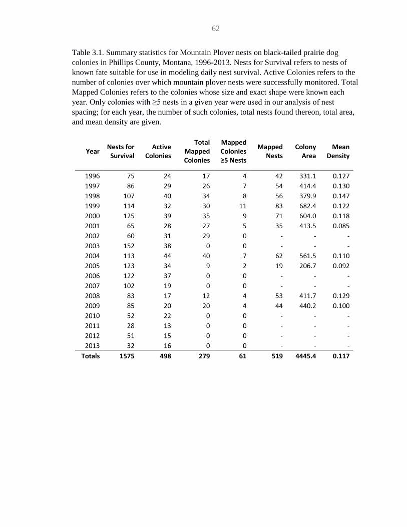
62

Table 3.1. Summary statistics for Mountain Plover nests on black-tailed prairie dog

colonies in Phillips County, Montana, 1996-2013. Nests for Survival refers to nests of

known fate suitable for use in modeling daily nest survival. Active Colonies refers to the

number of colonies over which mountain plover nests were successfully monitored. Total

Mapped Colonies refers to the colonies whose size and exact shape were known each

year. Only colonies with ≥5 nests in a given year were used in our analysis of nest

spacing; for each year, the number of such colonies, total nests found thereon, total area,

and mean density are given.

Year Nests for

Survival Active

Colonies

Total Mapped Colonies

Mapped Colonies ≥5 Nests

Mapped Nests

Colony Area

Mean Density

1996 75 24 17 4 42 331.1 0.127

1997 86 29 26 7 54 414.4 0.130

1998 107 40 34 8 56 379.9 0.147

1999 114 32 30 11 83 682.4 0.122

2000 125 39 35 9 71 604.0 0.118

2001 65 28 27 5 35 413.5 0.085

2002 60 31 29 0 - - -

2003 152 38 0 0 - - -

2004 113 44 40 7 62 561.5 0.110

2005 123 34 9 2 19 206.7 0.092

2006 122 37 0 0 - - -

2007 102 19 0 0 - - -

2008 83 17 12 4 53 411.7 0.129

2009 85 20 20 4 44 440.2 0.100

2010 52 22 0 0 - - -

2011 28 13 0 0 - - -

2012 51 15 0 0 - - -

2013 32 16 0 0 - - -

Totals 1575 498 279 61 519 4445.4 0.117

63

Table 3.2. Results of the analysis of Mountain Plover nest placement within actual prairie dog colony boundaries, Phillips

County, Montana, 1996-2009. The L function (upper section) evaluates the proportion of all pairwise inter-nest distances

smaller than some distance t, standardized to the estimated intensity λ; the G function (lower section) evaluates only the

proportion of nearest-neighbor distances less than t. For each year, 99 patterns of n nests each were placed randomly within the

combined boundaries of x colonies; the L or G function was evaluated across various ranges of distances and compared to the

mean value across all iterations to produce a test statistic ui. P-values are defined as the rank of the test statistic of the observed

pattern compared to all 99 simulated patterns and divided by 100.

64

Mapped Colonies: ≥5 Nests

Mapped Nests

Colony Area

Average Density

P: 0-100m (L)

P: 100-200 m (L)

P: 200-300 m (L)

P: 300-400 m (L)

P: 400-500 m (L)

P: 0-375 m (L)

P: 0-500 m (L)

1996 4 42 331.1 0.127 0.028 0.260 0.187 0.032 0.045 0.066 0.041

1997 7 54 414.4 0.130 0.012 0.778 0.291 0.223 0.247 0.116 0.135

1998 8 56 379.9 0.147 0.144 0.885 0.634 0.142 0.044 0.339 0.134

1999 11 83 682.4 0.122 0.528 0.966 0.802 0.656 0.388 0.892 0.721

2000 9 71 604.0 0.118 0.358 0.402 0.830 0.454 0.563 0.589 0.624

2001 5 35 413.5 0.085 0.390 0.020 0.030 0.084 0.127 0.027 0.030

2004 7 62 561.5 0.110 0.040 0.195 0.709 0.417 0.267 0.232 0.245

2005 2 19 206.7 0.092 0.384 0.657 0.917 0.386 0.108 0.691 0.313

2008 4 53 411.7 0.129 0.418 0.126 0.148 0.687 0.671 0.242 0.361

2009 4 44 440.2 0.100 0.025 0.120 0.313 0.904 0.544 0.123 0.219

Mapped Colonies: ≥5 Nests

Mapped Nests

Colony Area

Average Density

P: 0-100m (G)

P: 100-200 m (G)

P: 200-300 m (G)

P: 300-400 m (G)

P: 400-500 m (G)

P: 0-375 m (G)

P: 0-500 m (G)

1996 4 42 331.1 0.127 0.001 0.001 0.002 0.287 0.93 0.001 0.001

1997 7 54 414.4 0.130 0.001 0.001 0.001 0.011 0.086 0.001 0.001

1998 8 56 379.9 0.147 0.001 0.001 0.001 0.014 0.126 0.001 0.001

1999 11 83 682.4 0.122 0.001 0.001 0.001 0.002 0.039 0.001 0.001

2000 9 71 604.0 0.118 0.001 0.001 0.001 0.001 0.036 0.001 0.001

2001 5 35 413.5 0.085 0.238 0.001 0.004 0.016 0.067 0.001 0.001

2004 7 62 561.5 0.110 0.001 0.001 0.001 0.005 0.056 0.001 0.001

2005 2 19 206.7 0.092 0.001 0.001 0.008 0.037 0.155 0.001 0.001

2008 4 53 411.7 0.129 0.001 0.001 0.001 0.032 0.185 0.001 0.001

2009 4 44 440.2 0.100 0.002 0.001 0.001 0.022 0.129 0.001 0.001

65

Table 3.3. Estimated model parameters for spatial covariates included in well-supported

models of Mountain Plover nest survival in Phillips County, Montana. ΔAICc values are

relative to a model S(Group + TT + Age), which included separate intercepts for colony

geometry known and unknown, linear and quadratic time trends over the 79-day nesting

season, and a linear effect of nest age. Female, Male = number of contemporaneous

female- and male-tended nests within 375 m. Cent, InCent = prairie dog colony centroid

and internal centroid. Nearest = distance (m) to nearest contemporaneous nest. All =

number of contemporaneous nests within 375 m. Edge = distance (m) to prairie dog

colony boundary.

Parameter ΔAICc Model Weight

Estimate Standard Error

95% CI Lower

95% CI Upper

Female 0.004 0.145 -0.0746 0.0521 -0.1767 0.0274

InCent 1.190 0.080 -0.0002 0.0002 -0.0006 0.0002

Male 1.217 0.079 -0.0269 0.0301 -0.0859 0.0321

Cent 1.419 0.071 -0.0074 0.0096 -0.0263 0.0115

Nearest 1.798 0.059 -0.3321 0.7322 -0.0018 0.0011

All 1.850 0.058 0.0000 0.0000 -0.0001 0.0001

Edge 1.912 0.056 0.0000 0.0002 -0.0003 0.0002

66

Figure 3.1. Map of a subset of the study area from 2008 showing a typical arrangement of Mountain Plover nests (coded by sex of the

tending adult) on prairie dog colonies, Phillips County, Montana. Colony names (e.g., B-045) are also given.

67

0

0.5

1

1.5

2

2.5

3

3.5

4

4.5

5

0 100 200 300 400 500

1996 L(t)

0

0.5

1

1.5

2

2.5

3

3.5

4

4.5

0 100 200 300 400 500

1997 L(t)

0

0.5

1

1.5

2

2.5

3

3.5

4

4.5

0 100 200 300 400 500

1998 L(t)

0

0.5

1

1.5

2

2.5

3

3.5

4

4.5

0 100 200 300 400 500

1999 L(t)

0

0.5

1

1.5

2

2.5

3

3.5

4

4.5

0 100 200 300 400 500

2000 L(t)

0

0.5

1

1.5

2

2.5

3

3.5

4

4.5

5

0 100 200 300 400 500

2001 L(t)

68

Figure 3.2. Actual values of L(t) computed from mapped colonies with ≥5 Mountain

Plover nests from Phillips County, Montana, 1996–2009. The actual values of L(t) (black

line) are plotted against simulation envelopes (shaded region) spanning maximum and

minimum values of L(t) computed at 5 m intervals from 0 to 500 m from 999 patterns of

randomly placed points within the same colony boundaries. Large values of L(t) imply

more aggregated patterns while smaller values of L(t) imply more regular patterns. Please

note uneven vertical axes, as L(t) is scaled to estimated intensity (λ), which differs by

year.

0

0.5

1

1.5

2

2.5

3

3.5

4

4.5

5

0 100 200 300 400 500

2004 L(t)

0

1

2

3

4

5

6

0 100 200 300 400 500

2005 L(t)

0

0.5

1

1.5

2

2.5

3

3.5

4

4.5

5

0 100 200 300 400 500

2008 L(t)

0

1

2

3

4

5

6

0 100 200 300 400 500

2004 L(t)

69

0.0

0.2

0.4

0.6

0.8

1.0

0 100 200 300 400 500

1996 G(t)

0.0

0.2

0.4

0.6

0.8

1.0

0 100 200 300 400 500

1997 G(t)

0.0

0.2

0.4

0.6

0.8

1.0

0 100 200 300 400 500

1998 G(t)

0.0

0.2

0.4

0.6

0.8

1.0

0 100 200 300 400 500

1999 G(t)

0.0

0.2

0.4

0.6

0.8

1.0

0 100 200 300 400 500

2000 G(t)

0.0

0.2

0.4

0.6

0.8

1.0

0 100 200 300 400 500

2001 G(t)

70

Figure 3.3. Actual values of G(t) computed from mapped colonies with ≥5 Mountain

Plover nests from Phillips County, Montana, 1996–2009. Actual values (black line) are

plotted against simulation envelopes (shaded region) spanning maximum and minimum

values of G(t) computed at 5 m intervals from 0 to 500 m from 999 patterns of randomly

placed points within the same colony boundaries. Values of G(t) larger than the simulated

maximum imply aggregation while those below the simulated minimum imply inhibition.

0.0

0.2

0.4

0.6

0.8

1.0

0 100 200 300 400 500

2004 G(t)

0.0

0.2

0.4

0.6

0.8

1.0

0 100 200 300 400 500

2005 G(t)

0.0

0.2

0.4

0.6

0.8

1.0

0 100 200 300 400 500

2008 G(t)

0.0

0.2

0.4

0.6

0.8

1.0

0 100 200 300 400 500

2009 G(t)

71

Appendix. Results of our analysis of nest placement as a function of colony area, Phillips County, Montana, 1996-2012. The L

function summarizes the proportion of all pairwise inter-nest distances smaller than some distance t, standardized to the estimated

intensity λ; the G function evaluates only the proportion of nearest-neighbor distances less than t. For each colony-year combination,

999 patterns of n nests each were placed randomly within a square of equivalent area; the L or G function was evaluated across

various ranges of distances and compared to the its mean value across all iterations to produce a test statistic ui. P-values are defined

as the rank of the test statistic of the observed pattern compared to all 999 simulated patterns divided by 1000. Some colony-year areas

were estimated as the mean area across all known colony-years, 31.63 ha; these are denoted with asterisks (*).

Colony - Year Nests Area (ha)

Est. Density

(Nests/ha)

P: 0-100m (L)

P: 100-200 m (L)

P: 200-300 m (L)

P: 300-400 m (L)

P: 400-500 m (L)

P: 0-375 m (L)

P: 0-500 m (L)

B-040 1996 17 78.8 0.216 0.046 0.228 0.835 0.848 0.923 0.297 0.450

B-041 1996 11 40.5 0.272 0.194 0.059 0.003 0.001 0.001 0.003 0.001

B-043 1996 5 35.6 0.141 0.798 0.184 0.040 0.001 0.004 0.026 0.008

B-065 1996 6 0.7 8.696 0.001 0.001 0.001 0.001 0.001 0.001 0.001

B-083 1996 5 92.0 0.054 1.000 0.839 0.801 0.171 0.027 0.589 0.191

B-040 1997 16 76.2 0.210 0.211 0.326 0.586 0.479 0.329 0.455 0.430

B-041 1997 7 50.4 0.139 0.497 0.364 0.507 0.135 0.011 0.399 0.109

B-043 1997 6 48.7 0.123 0.742 0.628 0.747 0.428 0.704 0.749 0.801

B-049 1997 5 35.0 0.143 0.781 0.045 0.001 0.001 0.001 0.002 0.001

B-072 1997 6 33.5 0.179 0.624 0.895 0.994 0.344 0.058 0.879 0.587

B-148 1997 6 40.1 0.150 0.645 0.721 0.596 0.383 0.971 0.676 0.762

B-150 1997 5 39.2 0.128 0.970 0.748 0.478 0.888 1.000 0.886 0.931

B-040 1998 9 73.6 0.122 0.397 0.353 0.861 0.493 0.081 0.594 0.306

B-041 1998 7 94.3 0.074 0.930 0.113 0.271 0.088 0.014 0.115 0.050

B-071 1998 6 15.1 0.399 0.953 0.448 0.040 0.001 0.001 0.069 0.029

B-072 1998 5 27.0 0.185 0.722 0.919 0.986 0.599 0.139 0.944 0.901

B-150 1998 7 47.2 0.148 0.436 0.061 0.768 0.419 0.204 0.190 0.198

72

S-020 1998 7 19.0 0.368 0.063 0.661 0.155 0.006 0.001 0.076 0.015

B-026 1999 6 60.7 0.099 0.160 0.545 0.466 0.508 0.751 0.491 0.588

B-036 1999 7 75.6 0.093 0.831 0.134 0.418 0.617 0.651 0.294 0.371

B-040 1999 11 86.9 0.127 0.984 0.777 0.859 0.915 0.636 0.989 0.977

B-041 1999 7 106.3 0.066 0.971 0.113 0.008 0.004 0.002 0.004 0.003

B-071 1999 5 15.8 0.317 0.339 0.353 0.419 0.011 0.001 0.221 0.080

B-072 1999 5 36.4 0.137 0.917 0.495 0.954 0.794 0.301 0.848 0.795

B-118 1999 6 41.6 0.144 0.246 0.488 0.511 0.926 0.657 0.681 0.727

B-148 1999 7 48.4 0.145 0.540 0.490 0.487 0.501 0.385 0.588 0.588

B-150 1999 8 56.1 0.143 0.679 0.467 0.024 0.056 0.278 0.079 0.094

S-020 1999 5 20.3 0.246 0.439 0.569 0.731 0.074 0.001 0.581 0.210

B-026 2000 6 68.0 0.088 0.083 0.019 0.026 0.064 0.447 0.016 0.027

B-040 2000 14 63.5 0.220 0.382 0.091 0.005 0.028 0.022 0.020 0.017

B-041 2000 12 126.4 0.095 0.359 0.018 0.306 0.735 0.791 0.088 0.156

B-072 2000 6 45.5 0.132 0.650 0.138 0.653 0.790 0.833 0.344 0.445

B-077 2000 5 33.7 0.148 1.000 0.741 0.132 0.969 0.571 0.474 0.517

B-083 2000 5 34.2 0.146 0.709 0.044 0.067 0.035 0.622 0.027 0.037

B-118 2000 7 45.6 0.153 0.441 0.156 0.096 0.078 0.072 0.120 0.076

B-150 2000 9 65.1 0.138 0.460 0.556 0.984 0.991 0.985 0.809 0.897

B-026 2001 6 48.3 0.124 0.293 0.937 0.313 0.330 0.311 0.559 0.531

B-041 2001 8 153.2 0.052 1.000 0.143 0.027 0.114 0.537 0.051 0.071

B-118 2001 6 47.5 0.126 0.756 0.242 0.681 0.637 0.604 0.498 0.578

B-150 2002 6 77.4 0.077 1.000 0.140 0.398 0.870 0.853 0.293 0.407

B-040 2003 7 54.6 0.128 0.563 0.010 0.014 0.113 0.012 0.016 0.014

B-041 2003 26 173.0 0.150 0.297 0.364 0.591 0.667 0.752 0.561 0.696

B-042 2003 7 30.6 0.229 0.222 0.002 0.001 0.001 0.001 0.001 0.001

B-069 2003 8 66.5 0.120 0.682 0.683 0.025 0.015 0.020 0.047 0.036

B-071 2003 6 14.6 0.411 0.743 0.171 0.840 0.909 0.071 0.509 0.501

73

B-072 2003 18 128.9 0.140 0.743 0.256 0.045 0.041 0.139 0.071 0.071

B-077 2003 7 51.0 0.137 0.529 0.005 0.021 0.001 0.004 0.001 0.001

B-081 2003 5 67.8 0.074 1.000 0.493 0.254 0.365 0.311 0.412 0.418

B-148 2003 10 74.6 0.134 0.222 0.446 0.579 0.946 0.568 0.553 0.638

B-189 2003 5 30.9 0.162 0.694 0.043 0.122 0.002 0.001 0.025 0.005

B-041 2004 5 177.0 0.028 1.000 0.910 0.266 0.236 0.579 0.278 0.321

B-045 2004 6 27.6 0.217 0.371 0.149 0.007 0.006 0.001 0.016 0.002

B-065 2004 6 61.1 0.098 0.907 0.080 0.057 0.256 0.236 0.083 0.099

B-069 2004 9 75.1 0.120 0.957 0.785 0.103 0.071 0.125 0.228 0.166

B-072 2004 16 104.0 0.154 0.204 0.166 0.510 0.461 0.312 0.311 0.307

B-077 2004 7 49.6 0.141 0.470 0.183 0.246 0.196 0.692 0.201 0.264

B-148 2004 8 67.1 0.119 0.924 0.375 0.824 0.770 0.604 0.766 0.810

B-041 2005 11 173.6 0.063 0.773 0.229 0.216 0.710 0.362 0.343 0.378

B-042 2005 6 33.1 0.181 0.798 0.560 0.075 0.050 0.003 0.156 0.071

B-049 2005 6 56.0 0.107 0.800 0.042 0.004 0.283 0.306 0.008 0.015

B-065 2005 6 41.2 0.145 0.607 0.014 0.005 0.001 0.001 0.001 0.001

B-066 2005 10 40.4 0.248 0.113 0.253 0.041 0.090 0.021 0.048 0.036

B-072 2005 10 2.7 3.663 0.001 0.001 0.001 0.001 0.001 0.001 0.001

B-120 2005 7 26.6 0.263 0.142 0.003 0.044 0.021 0.002 0.004 0.003

B-150 2005 7 81.1 0.086 0.775 0.417 0.176 0.154 0.217 0.266 0.241

B-041 2006 17 199.4 0.085 0.631 0.338 0.014 0.014 0.014 0.020 0.014

B-065 2006 7 21.4 0.327 0.097 0.001 0.001 0.001 0.001 0.001 0.001

B-066 2006 5 22.1 0.226 0.507 0.009 0.001 0.003 0.001 0.001 0.001

B-069 2006 11 85.1 0.129 0.195 0.320 0.416 0.223 0.286 0.274 0.276

B-150 2006 9 82.3 0.109 1.000 0.746 0.199 0.329 0.558 0.489 0.547

CMR-Man 2006 10 10.2 0.980 0.001 0.001 0.001 0.001 0.001 0.001 0.001

B-041 2007 48 225.3 0.213 0.023 0.530 0.635 0.775 0.289 0.335 0.329

B-069 2007 15 96.5 0.155 0.046 0.083 0.509 0.440 0.669 0.126 0.225

74

B-041 2008 27 211.6 0.128 0.319 0.130 0.180 0.587 0.930 0.225 0.347

B-045 2008 9 46.2 0.195 0.284 0.620 0.204 0.027 0.012 0.140 0.049

B-069 2008 13 108.6 0.120 0.484 0.616 0.178 0.625 0.764 0.455 0.593

B-072 2008 5 48.3 0.103 0.938 0.644 0.570 0.117 0.033 0.517 0.293

S-010 2008 8 43.2 0.185 0.225 0.017 0.724 0.505 0.654 0.078 0.112

B-041 2009 17 213.6 0.080 0.527 0.849 0.567 0.035 0.013 0.249 0.058

B-042 2009 5 12.7 0.393 0.166 0.001 0.001 0.001 0.001 0.001 0.001

B-069 2009 10 114.6 0.087 0.518 0.202 0.230 0.055 0.120 0.123 0.099

B-072 2009 8 58.6 0.136 0.417 0.126 0.018 0.059 0.003 0.037 0.016

B-148 2009 9 48.3 0.186 0.608 0.779 0.708 0.700 0.755 0.871 0.900

S-010 2009 6 53.5 0.112 0.818 0.346 0.957 0.934 0.553 0.701 0.735

B-041 2010 8 31.63* 0.253 0.095 0.010 0.001 0.001 0.001 0.001 0.001

B-083 2010 6 31.63* 0.190 0.432 0.004 0.001 0.001 0.001 0.003 0.001

S-010 2010 5 31.63* 0.158 0.730 0.032 0.001 0.001 0.005 0.001 0.001

B-041 2011 5 31.63* 0.158 0.716 0.356 0.374 0.780 0.814 0.529 0.585

S-010 2011 10 31.63* 0.316 0.009 0.001 0.006 0.010 0.002 0.001 0.001

B-077 2012 6 31.63* 0.190 0.975 0.903 0.947 0.906 0.697 0.999 0.996

B-189 2012 5 31.63* 0.158 0.755 0.056 0.029 0.001 0.001 0.009 0.003

S-010 2012 9 31.63* 0.285 0.772 0.004 0.002 0.026 0.008 0.004 0.003

75

Colony - Year Nests Area (ha)

Est. Density

(Nests/ha)

P:0-100m

(G)

P:100-200m

(G)

P:200-300m

(G)

P:300-400m

(G)

P:400-500m

(G)

P:0-375 m (G)

P:0-500 m (G)

B-040 1996 17 78.8 0.216 0.107 0.007 0.205 1.000 1.000 0.011 0.011

B-041 1996 11 40.5 0.272 0.006 0.019 0.409 1.000 1.000 0.003 0.003

B-043 1996 5 35.6 0.141 0.763 0.230 0.977 0.118 0.011 0.352 0.237

B-065 1996 6 0.7 8.696 0.001 0.001 0.001 0.001 0.001 0.001 0.001

B-083 1996 5 92.0 0.054 1.000 0.049 0.073 0.261 0.566 0.053 0.060

B-040 1997 16 76.2 0.210 0.133 0.010 0.229 1.000 1.000 0.019 0.019

B-041 1997 7 50.4 0.139 0.488 0.020 0.227 0.799 1.000 0.035 0.035

B-043 1997 6 48.7 0.123 0.709 0.293 0.551 0.371 0.272 0.489 0.504

B-049 1997 5 35.0 0.143 0.742 0.045 0.002 1.000 1.000 0.002 0.002

B-072 1997 6 33.5 0.179 0.132 0.041 0.293 1.000 1.000 0.066 0.068

B-148 1997 6 40.1 0.150 0.127 0.018 0.258 0.715 1.000 0.047 0.047

B-150 1997 5 39.2 0.128 0.296 0.119 0.223 0.683 1.000 0.148 0.160

B-040 1998 9 73.6 0.122 0.406 0.005 0.129 0.441 1.000 0.022 0.022

B-041 1998 7 94.3 0.074 0.866 0.056 0.040 0.311 0.840 0.075 0.085

B-071 1998 6 15.1 0.399 0.317 0.974 0.226 1.000 1.000 0.584 0.584

B-072 1998 5 27.0 0.185 0.774 0.132 0.536 1.000 1.000 0.234 0.238

B-150 1998 7 47.2 0.148 0.461 0.077 0.432 0.700 1.000 0.130 0.137

S-020 1998 7 19.0 0.368 0.094 0.385 1.000 1.000 1.000 0.138 0.138

B-026 1999 6 60.7 0.099 0.031 0.025 0.221 0.571 0.671 0.043 0.048

B-036 1999 7 75.6 0.093 0.781 0.212 0.308 0.412 0.715 0.273 0.292

B-040 1999 11 86.9 0.127 0.001 0.001 0.097 0.428 1.000 0.001 0.001

B-041 1999 7 106.3 0.066 0.898 0.148 0.006 0.010 0.918 0.004 0.004

B-071 1999 5 15.8 0.317 0.363 0.512 0.052 0.002 0.001 0.182 0.115

B-072 1999 5 36.4 0.137 0.034 0.011 0.315 0.744 0.767 0.023 0.023

76

B-118 1999 6 41.6 0.144 0.032 0.135 0.561 0.988 1.000 0.076 0.080

B-148 1999 7 48.4 0.145 0.142 0.046 0.199 0.981 1.000 0.076 0.079

B-150 1999 8 56.1 0.143 0.015 0.038 0.853 0.942 1.000 0.027 0.027

S-020 1999 5 20.3 0.246 0.458 0.400 0.185 0.008 0.001 0.291 0.149

B-026 2000 6 68.0 0.088 0.001 0.001 0.120 0.255 0.620 0.001 0.001

B-040 2000 14 63.5 0.220 0.001 0.095 0.785 0.133 1.000 0.002 0.002

B-041 2000 12 126.4 0.095 0.377 0.041 0.071 0.281 0.984 0.041 0.044

B-072 2000 6 45.5 0.132 0.648 0.089 0.228 0.444 0.884 0.132 0.136

B-077 2000 5 33.7 0.148 0.062 0.006 0.393 0.412 1.000 0.035 0.036

B-083 2000 5 34.2 0.146 0.710 0.040 0.360 1.000 1.000 0.071 0.076

B-118 2000 7 45.6 0.153 0.457 0.177 0.261 0.711 1.000 0.216 0.221

B-150 2000 9 65.1 0.138 0.496 0.274 0.167 0.600 0.369 0.257 0.269

B-026 2001 6 48.3 0.124 0.025 0.259 0.826 0.287 1.000 0.131 0.140

B-041 2001 8 153.2 0.052 1.000 0.192 0.050 0.436 0.443 0.086 0.098

B-118 2001 6 47.5 0.126 0.715 0.059 0.236 0.835 1.000 0.096 0.102

B-150 2002 6 77.4 0.077 0.943 0.005 0.043 0.233 0.581 0.014 0.016

B-040 2003 7 54.6 0.128 0.566 0.010 0.013 0.921 1.000 0.007 0.007

B-041 2003 26 173.0 0.150 0.001 0.001 0.235 0.810 1.000 0.001 0.001

B-042 2003 7 30.6 0.229 0.273 0.006 0.266 0.115 1.000 0.008 0.008

B-069 2003 8 66.5 0.120 0.610 0.035 0.138 0.755 1.000 0.055 0.057

B-071 2003 6 14.6 0.411 0.143 0.647 0.347 1.000 1.000 0.246 0.246

B-072 2003 18 128.9 0.140 0.001 0.001 0.103 0.250 1.000 0.001 0.001

B-077 2003 7 51.0 0.137 0.520 0.005 0.232 0.888 1.000 0.017 0.017

B-081 2003 5 67.8 0.074 1.000 0.047 0.113 0.386 0.942 0.075 0.083

B-148 2003 10 74.6 0.134 0.269 0.039 0.124 0.771 1.000 0.055 0.055

B-189 2003 5 30.9 0.162 0.671 0.044 0.487 0.064 0.040 0.067 0.066

B-041 2004 5 177.0 0.028 1.000 0.877 0.312 0.383 0.957 0.315 0.413

B-045 2004 6 27.6 0.217 0.393 0.240 0.228 0.129 1.000 0.316 0.316

77

B-065 2004 6 61.1 0.098 0.848 0.093 0.166 0.959 0.352 0.121 0.130

B-069 2004 9 75.1 0.120 0.002 0.001 0.079 0.228 0.638 0.001 0.001

B-072 2004 16 104.0 0.154 0.429 0.045 0.096 0.757 1.000 0.060 0.060

B-077 2004 7 49.6 0.141 0.491 0.247 0.728 0.681 0.588 0.388 0.398

B-148 2004 8 67.1 0.119 0.030 0.012 0.134 0.584 1.000 0.018 0.018

B-041 2005 11 173.6 0.063 0.044 0.001 0.010 0.099 0.504 0.001 0.001

B-042 2005 6 33.1 0.181 0.774 0.715 0.813 0.033 0.002 0.714 0.433

B-049 2005 6 56.0 0.107 0.738 0.051 0.004 0.844 0.899 0.007 0.008

B-065 2005 6 41.2 0.145 0.609 0.013 0.014 0.647 1.000 0.011 0.011

B-066 2005 10 40.4 0.248 0.092 0.086 0.709 1.000 1.000 0.080 0.080

B-072 2005 10 2.7 3.663 0.001 0.001 0.001 1.000 1.000 0.001 0.001

B-120 2005 7 26.6 0.263 0.201 0.001 0.756 1.000 1.000 0.002 0.002

B-150 2005 7 81.1 0.086 0.749 0.078 0.382 0.551 0.711 0.145 0.156

B-041 2006 17 199.4 0.085 0.687 0.003 0.014 0.132 0.536 0.003 0.003

B-065 2006 7 21.4 0.327 0.128 0.001 0.464 1.000 1.000 0.001 0.001

B-066 2006 5 22.1 0.226 0.519 0.008 0.001 0.253 1.000 0.001 0.001

B-069 2006 11 85.1 0.129 0.242 0.006 0.137 0.309 0.611 0.017 0.018

B-150 2006 9 82.3 0.109 0.005 0.015 0.079 0.312 0.475 0.004 0.004

CMR-Man 2006 10 10.2 0.980 0.001 0.001 0.001 0.001 0.001 0.001 0.001

B-041 2007 48 225.3 0.213 0.001 0.001 0.053 0.905 0.127 0.001 0.001

B-069 2007 15 96.5 0.155 0.086 0.102 0.109 0.795 1.000 0.069 0.070

B-041 2008 27 211.6 0.128 0.001 0.001 0.012 0.292 1.000 0.001 0.001

B-045 2008 9 46.2 0.195 0.047 0.025 0.217 0.321 1.000 0.025 0.025

B-069 2008 13 108.6 0.120 0.001 0.001 0.064 0.522 1.000 0.001 0.001

B-072 2008 5 48.3 0.103 0.911 0.287 0.265 0.766 1.000 0.274 0.290

S-010 2008 8 43.2 0.185 0.258 0.040 0.530 1.000 1.000 0.073 0.073

B-041 2009 17 213.6 0.080 0.002 0.001 0.008 0.115 0.304 0.001 0.001

B-042 2009 5 12.7 0.393 0.195 0.001 1.000 1.000 1.000 0.001 0.001

78

B-069 2009 10 114.6 0.087 0.520 0.367 0.371 0.896 0.278 0.490 0.512

B-072 2009 8 58.6 0.136 0.432 0.481 0.445 0.809 1.000 0.526 0.535

B-148 2009 9 48.3 0.186 0.013 0.034 0.229 0.474 1.000 0.012 0.012

S-010 2009 6 53.5 0.112 0.782 0.068 0.132 0.378 0.301 0.091 0.101

B-041 2010 8 31.63* 0.253 0.146 0.009 0.669 1.000 1.000 0.024 0.024

B-083 2010 6 31.63* 0.190 0.439 0.002 0.001 0.646 1.000 0.001 0.001

S-010 2010 5 31.63* 0.158 0.696 0.025 0.001 0.001 0.173 0.001 0.001

B-041 2011 5 31.63* 0.158 0.704 0.101 0.410 1.000 1.000 0.148 0.151

S-010 2011 10 31.63* 0.316 0.018 0.001 0.198 1.000 1.000 0.001 0.001

B-077 2012 6 31.63* 0.190 0.043 0.097 0.449 0.437 1.000 0.065 0.066

B-189 2012 5 31.63* 0.158 0.728 0.063 0.804 0.193 1.000 0.121 0.123

S-010 2012 9 31.63* 0.285 0.008 0.512 0.379 1.000 1.000 0.043 0.043

79

CHAPTER 4

SURVIVAL OF DEPENDENT MOUNTAIN PLOVER (CHARADRIUS MONTANUS)

CHICKS IN MONTANA

A paper to be submitted to The Wilson Journal of Ornithology



Ames, IA 50011, USA

Abstract

The survival of dependent offspring is a critical aspect of recruitment and overall

population growth. Understanding the factors that influence chick survival in birds is

important if we are to effectively manage species of conservation concern. We

constructed models of chick survival for a population of Mountain Plovers (Charadrius

montanus) using counts of unmarked chicks seen with uniquely marked adults. Our best

models showed a nonlinear decreasing trend in daily chick survival over the brood

period, which conflicts with earlier findings for this species. However, our estimates of

overall survival were congruous with previous studies. Our estimates of daily survival

ranged from 0.998 (SD = 0.001; 95% CI = 0.997, 0.999) at chick age = 1 to 0.966 (SD =

0.23, 95% CI = 0.920, 0.998) at chick age = 35 (Table 3). Cumulative survival across the

brood period was estimated as 0.746 (range 0.550 to 0.948). Although our best model

included effects of chick age, day of season, temperature, precipitation, and year, none of

the covariate effects were well estimated except some individual year effects. We

conclude that the survival of chicks is primarily a function of annual variation, and may

be further influenced by temperature, day of season, precipitation, and chick age. Our

inability to construct an effective predictive model of chick survival likely stems from

both the data set and limitations inherent in this modeling approach.

Introduction

The survival of dependent offspring is directly tied to reproductive success and

recruitment and may have far-reaching consequences for a species’ population growth

and future prospects. To successfully monitor and manage species of concern it is critical

that we accurately estimate survival rates at all stages in an animal’s life history,

determine the factors driving these rates, and assess their influence on population

dynamics. Survival rates vary depending on an animal’s age or life history stage and we

80

can easily build models that reflect this variation (Pollock 1981). The ability to estimate

these different rates enables us to assess the relative importance of each age or stage to

overall population growth rate using elasticity analysis (Caswell 1978, 1984), which may

allow more effective targeting of management actions.

Dinsmore et al. (2010) recently analyzed factors influencing the stochastic

population growth rate of the Mountain Plover (Charadrius montanus), a cryptic, ground-

nesting migratory shorebird endemic to the great plains region of North America. Using

elasticity analysis, they determined that survival of chicks was a significant factor in the

population growth of Mountain Plovers in multiple regions and recommended increased

chick survival as a suitable target for increasing population growth in this species

(Dinsmore et al. 2010). Our goal in the present study was to investigate and model the

survival of dependent Mountain Plover chicks on black-tailed prairie dog (Cynomys

ludovicianus) colonies in southern Phillips County, Montana based on resightings of

uniquely marked adults. The Mountain Plover is a long-lived, iteroparous species (Knopf

and Wunder 2006) and the use of marked adults to estimate chick survival allows us to

make use of a larger sample than would be feasible by uniquely marking chicks. This

population provides an opportunity to explore a variety of potential influences on chick

survival, including sex of the tending parent, size of the prairie dog colony, the presence

and density of other broods occupying the same colony, drought and temperature

conditions, linear and non-linear time trends across the breeding season, and annual

variation due to environmental factors beyond the scope of the data.

Several studies have already examined chick survival in the Mountain Plover.

Miller and Knopf (1993) and Knopf and Rupert (1996) marked chicks individually and

81

used radiotelemetry to estimate chick survival in Mountain Plover populations in

Colorado. Dinsmore and Knopf (2005) used radiotagged adults to estimate survival of

unmarked chicks on prairie dog colonies in Montana. Lukacs et al. (2004) developed a

maximum-likelihood based model for estimating the survival of unmarked chicks based

on resighting of marked adults; this study also relied on radiotelemetry to locate the

broods. Dreitz (2009) applied the Lukacs et al. (2004) model to a larger sample of radio-

tagged adults tending broods in Colorado. Radiotelemetry provides a reliable means of

locating and tracking individuals; however, these methods must be incorporated at the

study design stage.

We wanted to investigate chick survival using a large preexisting set of banding

and resighting data for the Phillips County population of Mountain Plovers. These data

are more extensive than those used in previous studies, comprising data on >500 unique

broods across a 20-year study period, and also include useful ancillary data about

individual nests, prairie dog colonies, weather, drought, and other covariates. The

downside of this approach is that visual resighting is probably a less reliable way to

relocate brooding adults; this results in fewer resightings at longer intervals, decreasing

the precision of our daily chick survival estimates (Lukacs et al. 2004). Our objective is

to test the utility of this long-term dataset for estimating Mountain Plover chick survival,

and to investigate the influence of several biologically relevant factors on observed

survival patterns.

82

Methods

Study species

The Mountain Plover is a cryptic, migratory, ground-nesting shorebird endemic to

arid landscapes of western North America, most commonly found in prairie, scrubland

and semi-desert (Knopf and Wunder 2006). The majority of the population occupies a

broad swath running north-south through Montana, Wyoming, and Colorado, with the

latter state considered the continental stronghold (Graul and Webster 1976). In parts of its

range the Mountain Plover nests preferentially on prairie dog (Cynomys sp.) colonies or

other heavily grazed land, and it is generally considered a species of disturbed habitats

(Knopf and Wunder 2006). The Mountain Plover has an unusual breeding system in

which the female divides her clutch between two separate nests. Mean clutch size is 6

eggs; 3 are deposited in a nest tended by the male and 3 in a second nest tended by the

female (Graul 1973, 1975). Incubation begins with the laying of the final egg in each nest

(Graul 1975, Dinsmore et al. 2002). Incubating Mountain Plovers typically leave the nest

to forage 1-2 times per hour during daylight hours, with an average off-bout duration of

<15 minutes (Skrade and Dinsmore 2012). Graul (1975) reports incubating adults spent

42.3% and 57.8% of time on the nest during daylight hours in two non-consecutive years

and posits that the difference may have been a function of temperature, as the latter year

was warmer. Incubation lasts an average of 29 days and fledging typically occurs at 33-

34 days after hatch; chicks remain with their tending parent until fledging (Graul 1975).



Knopf and Wunder 2006) and the current continental population is estimated at 11,000-

83






current range.

Although there have been no detailed studies on cause-specific mortality in

Mountain Plover chicks, losses are generally attributed to predation or exposure. Chicks

are vulnerable to predation by a number of species, including red fox (Vulpes vulpes),

swift fox (V. velox), coyote (Canis latrans), Loggerhead Shrike (Lanius ludovicianus),

Prairie Falcon (Falco mexicanus), Swainson’s Hawk (Buteo swainsonii), Northern

Harrier (Circus cyaneus), prairie rattlesnake (Crotalus viridis), and others (Graul 1975,

Miller and Knopf 1993, May 2001, Knopf and Wunder 2006). Chicks may also succumb

to excessive heat or inclement weather (Graul 1975).

Study area

We collected data on plover broods in a 3000 km2 region of southern Phillips

County in north-central Montana between 1995 and 2013. The study area comprises

mostly public land administered by the Bureau of Land Management and the Charles M.

Russell National Wildlife Refuge, administered by the U.S. Fish and Wildlife Service

(Dinsmore et al. 2002). Land cover consists of mixed-grass prairie and sagebrush flats

interspersed with black-tailed prairie dog (C. ludovicianus) colonies, which have a unique

vegetation structure due to the prairie dogs’ grazing activity (Dinsmore et al. 2003).

Breeding Mountain Plovers in Montana are strongly associated with black-tailed prairie

84

dog colonies (Knowles et al. 1982, Knowles and Knowles 1984) and the majority of our

data were collected on such colonies.

Searching and monitoring

We used live resighting data for Mountain Plovers raising broods on active prairie

dog colonies in the study area during the May-July breeding season. All known active

black-tailed prairie dog colonies in the study area were systematically searched ≥3 times

per year for plover nests. We conducted nest searches by vehicle and searched colonies

systematically by driving an approximately 50 m grid that ensured complete colony

coverage. If an adult plover was sighted it was then watched until it returned to a nest or

offered behavioral cues (SJD, pers. comm.) that indicated it did not have a nest. The

location of each nest was marked upon discovery, and we captured the tending adult(s)

using walk-in traps placed over their nests to band them and take morphometric

measurements and feather samples (Dinsmore et al. 2002). We used feather samples to

sex adults using molecular methods, which were effective in sexing some 85% of adults.

Dinsmore et al. (2002) developed an egg floatation model for this species, and by floating

eggs on discovery we were able to age most nests to an accuracy of 1-2 days and predict

hatch date. Following hatch, we resighted adult plovers at intervals of ~7 days.

Local biologists collected all prairie dog colony data (John Grensten, pers.

comm.), which are available for most colonies from 1995 through 2007. Colony area was

calculated by tracing the perimeter of the colony with a handheld GPS unit and

converting this information to polygon data in ArcGIS, allowing the colony area (in

hectares) to be calculated. All colonies within the study area were mapped in 1998, 2000,

2002, 2004, and 2007; in other years only a portion of colonies were actually mapped

85

while areas of other colonies were estimated by extrapolation (Dinsmore and Smith

2010). For years in which some colony sizes were known and others unknown, unknown

colony sizes were coded as the average colony size for that year. For years in which no

colony sizes were known (2010-2013) we coded all colony sizes as the average across all

years, 31.63 ha.

Weather data included daily high temperature and precipitation. For simplicity,

we assumed weather was uniform across the study area and within any given day. We

obtained weather data directly from a local National Weather Service-recognized weather

station (Dale Veseth, pers. comm.) located in the center of the study area. Daily

temperature and precipitation data were not available for all days across the 19-year study

period; we interpolated missing data by taking the mean of the day immediately before

and after the missing information. Data on historical drought indices were obtained from

the National Oceanic and Atmospheric Administration’s Gridded Climate Divisional

Dataset (CLIMDIV) for Montana’s North Central division. These included Palmer

Drought Severity Index (PDSI) and Palmer Modified Drought Index (PMDI).

Analysis

Lukacs et al. (2004) developed a model for estimating the survival of unmarked

dependent young based on resighting of marked adults and allowing for imperfect

detection, which has since been integrated into Program MARK (White and Burnham

1999). This model considers chicks within each brood exchangeable and estimates two

parameters: φi, the probability that a chick will survive from time i to time i+1, and pi, the

probability that a chick will be detected, given that it is alive and that its parent is

detected at time i (Lukacs et al. 2004). Both parameters can be modeled as functions of

86

various individual, group, and temporal covariates using a number of link functions

(Lukacs et al. 2004). This model makes several key assumptions: (1) broods are

independent of one another, (2) chicks do not move between broods and a brood can only

lose chicks, not gain them, (3) chicks within a brood have the same probability of

survival at a given time (i.e., there is no heterogeneity among chicks within broods), and

(4) at any given time, survival is equal among broods sharing identical covariate values

(Lukacs et al. 2004). Program MARK considers initial brood size to be the maximum

number of chicks observed at any occasion in the encounter history. As with other fully

time-dependent models with imperfect detection, the last φi and pi are confounded and

cannot be estimated separately (Lukacs et al. 2004).

We constructed the encounter history for each brood by querying a database of

colony surveys from any year in which an adult was observed with ≥1 chick or was

recorded as having a brood. Our encounter history covered the entire fledging period,

which we considered to be the 34 days after chicks hatched. The parameters of the

Lukacs model apply only to chicks; detection probability of chicks is conditioned on the

successful detection of the tending adult, so it is not necessary to estimate detection

probability for adults (Lukacs et al. 2004). We had to determine the age of the chicks to

accurately estimate the effect of aging on survival probability. In most cases, the marked

adult was associated with a marked nest from the same year, which we could safely

assume was the chicks’ natal nest. We floated eggs from all active nests upon discovery

to determine their age, from which we were able to predict hatch date. Some broods were

not associated with known nests, so we did not have an exact hatch date. However, these

broods were often captured and banded upon discovery and were consequently weighed.

87

Chick body mass is strongly correlated with age, so we were able to estimate age for

these broods using a logistic regression equation developed for this species (Dinsmore

2008).

Brood sightings were not always recorded consistently. Some resightings were

recorded simply as “brood;” we coded these encounters as 0 chicks, since the adult was

clearly seen, but chicks may not have been detected. Others were recorded with a degree

of uncertainty, e.g., “2+”; we treated these resightings conservatively, ignoring the plus

sign on the assumption it represents chicks that were never actually observed. These are

conservative choices and may bias our survival estimates low.

The dependent young survival model developed by Lukacs et al. (2004) estimates

survival of each chick in a given brood at age i and can incorporate continuous and

discrete covariates at the level of individual broods, temporal covariates at the scale of

days, weeks, months or years, and an arbitrary number of groups. We chose to include

the following covariates as potentially relevant to chick survival:

1) Sex of the tending adult. Dinsmore and Knopf (2005) found that dependent

chicks in female-tended broods had higher survival than those in male-tended broods,

apparently a tradeoff for higher nest survival in male-tended nests. We hypothesize that

male-tended broods will be associated with lower survival.

2) Size of the brood’s natal prairie dog colony. The primary role of parental

caregivers in precocial species is to lead their offspring to foraging grounds (Dreitz

2009). Brooding Mountain Plovers in Montana confine their movements to the colony on

which the nest was originally situated (Dinsmore 2002). A larger colony provides more

88

potential foraging areas, potentially increasing chick survival through better food

resources. However, larger colonies may also contain more neighboring broods,

increasing competition for high quality food resources and potentially lowering survival.

The concentration of breeding birds and prairie dogs may also attract predators. As most

losses of plover chicks appear to result from predation rather than starvation or

abandonment (Knopf and Wunder 2006), we predict that larger colonies will have lower

chick survival.

3) Palmer Drought Severity Index (PDSI) and Palmer Modified drought Index

(PMDI), a simple measure of environmental moisture deficiency (Palmer 1965) which is

now widely available as historical data for most of the country (NOAA 2016). Annual

average PDSI and PMDI were included for both the current year and the previous year,

since the effects of drought on vegetation and other organisms may persist beyond the

duration of the drought itself. The survival of adult Mountain Plovers does not decrease

during drought years (Dinsmore 2008) but reproductive success appears to be lower in

drought years (Knopf and Rupert 1996) so we hypothesize that chick survival will be

lower in years with more negative drought indices.

4) Average daily high temperature across the brood period. Mountain Plover

chicks are highly vulnerable to sun and heat, with young chicks succumbing to heat in as

little as 15 minutes when left exposed (Graul 1975). We predict that warmer temperatures

will produce a negative effect on chick survival.

5) Total precipitation across the brood period. Dinsmore et al. (2002) found a

negative effect of precipitation events on nest survival in Mountain Plovers; the proposed

explanation was that one of the primary nest predators of Mountain Plovers, the bull

89

snake (Pituophis catenifer) shows increased activity following rain. Chicks are also

potentially vulnerable to snakes and other olfactory predators; we hypothesize that total

rainfall will be negatively associated with chick survival.

6) Dummy variables representing years from 1995 through 2014. Survival may

vary by year in response to temporal factors not adequately reflected in climatic data. In

particular, the prairie dog colonies on which plovers nest are variable in size and activity

level from year to year due to the combined effects of prairie dog population growth and

periodic outbreaks of sylvatic plague (Dinsmore and Smith 2010). We expect survival to

be lower during and following years of plague outbreaks as the die-off of prairie dogs

causes a decrease in grazing activity which quickly renders the habitat less suitable for

plover breeding.

7) Number of successfully hatched nests on the same colony in the same year.

Mountain Plover broods move hundreds of meters per day (Knopf and Rupert 1996) and

their home range is directly related to the size of the prairie dog colony on which they

forage (Dreitz et al. 2005). We expect that the presence of competing broods may

constrain their movements and thus hamper their ability to forage effectively. Unrelated

adult Mountain Plovers and other birds have been observed attacking isolated Mountain

Plover chicks (Graul 1975) so the presence of competing broods may constitute a direct

threat to survival if chicks become separated from their parent. We hypothesize that

broods with more neighbors on the same colony will have lower survival.

8) Day of season values for occasion 1, 2, … 36, coded as Hatch + 0, Hatch + 1,

…, Hatch + 35. The best model tested by Dinsmore and Knopf (2005) included a

nonlinear trend in chick survival over the course of the breeding season, which we also

90

expect to find. Chick survival started low and increased quickly, then leveled off after

day 10-15 of the brood period (Dinsmore and Knopf 2005).. We predict that survival will

increase linearly or nonlinearly across the breeding season. This was the only temporally-

varying covariate included in our model.

We constructed models incorporating various combinations of these covariates

using the design matrix utility in Program MARK version 8.0 (White and Burnham 1999)

under the Lukacs Young Survival from Marked Adults model framework with a logit link

function. In keeping with Lukacs et al. (2004), we considered modeling all daily survival

probabilities with the same intercept, with one intercept for the first day and another

intercept for all days after the first, with separate intercepts for the first two days and

another intercept for all subsequent days, etc. Graul (1975) notes that mortality is greatest

in chicks <3 days old and appears constant for older chicks. We also attempted to include

linear and quadratic time trends across the brooding period, which translates to an effect

(whether linear or quadratic) of the age of the chicks. Sex and year were included as

categorical variables; sex was coded as a single digit (-1 = female, 0 = unknown, 1 =

male) and year was coded as 20 dummy variables coding for years 1995 through 2014

(1995 implicitly acted as the intercept for the model).

As an example, below is a line from the MARK input file containing the

information for a single brood. This information is for a bird with the color band

combination WOWB that was brooding chicks in 1997. The encounter history consists of

a string of 72 digits; each pair of digits represents a day during the brood period. A day

on which the adult was not observed is coded as ‘..’. A day on which the adult was

observed with no chicks is coded as ‘00’, with one chick as ‘01’, with two chicks as ‘02’,

91

with three chicks as ‘03’, and so forth, although our data set included no broods with >3

chicks. This individual was seen on the day of hatch with 0 chicks, on day 18 with 3

chicks, and on day 22 with 1 chick. Following the encounter history is a frequency code,

which is always 1 for data incorporating individual covariates. Following the frequency

code are the covariates: the 1 indicates that this bird is male; 48.73 is the colony area in

hectares; 18 is the day these chicks hatched. The next four columns are the Palmer

Drought Severity Index (PDSI) for the current and previous year and the Palmer

Modified Drought Index (PMDI) for the current and previous year. Following these are

the average daily high temperature (°F) over the entire brood period and the total

precipitation (inches) over the brood period. Finally there are 20 columns of dummy

variables representing years 1995 to 2014.

/* 1997 WOWB */

00................................03......01...........................

. 1 1 48.73 18 1.018 2.66 1.096 2.278 78.9 3.4 0

0 1 0 0 0 0 0 0 0 0 0

0 0 0 0 0 0 0 0 ;

We used Akaike’s Information Criterion with a correction for finite sample size

(AICc; Akaike 1973, Burnham and Anderson 2002) to select the best model. We

considered models with ΔAICc ≤2 to have good support from the data.

Program MARK was unable to estimate the standard error for all model

parameters (as can happen when parameter variances are too close to 0), so we used the

program’s Markov Chain Monte Carlo (MCMC) simulation utility to obtain better

estimates. We used the original MLE parameter estimates from the best model as starting

values. The simulation ran 4,000 iterations for tuning and 1,000 iterations as a ‘burn-in’

92

period, followed by 10,000 iterations to obtain the final estimates. Daily chick survival φi

and its standard error were estimated as the mean and standard deviation from the 10,000

retained samples of the MCMC simulation, which were based on the mean values of all

covariates. Cumulative chick survival was defined as ∏ 𝜑𝑖35𝑖=1 . Below we report the mean

parameter values, their standard deviations, and the Highest Probability Density (HPD)

95% credible intervals from this simulation.

Results

We based our analysis on a sample of 532 Mountain Plover broods that were

monitored between 1995 and 2014. The number of broods we detected varied by year

(Table 1), as did the average number of detections per brood, which is largely a function

of dedicated effort toward resighting broods during some years (1999, 2010) and not

others.

The best model of chick survival included effects of year, average daily high

temperature across the brood period, total precipitation across the brood period, and

linear and quadratic effects of both day of season and chick age. The only alternative

model with good support from the data (ΔAICc = 1.48) also included an effect of the

Palmer Drought Severity Index (PDSI) from the previous year. The point estimate for the

effect of PDSI was negative (indicating that wetter years are better for chick survival);

however, this parameter was not well estimated. Neither the best model nor the sole

competitive model included an effect of prairie dog colony size or number of neighboring

broods.

93

Predictors of chick survival

None of the individual covariates mentioned above had a strong effect on chick

survival; all 95% HPD credible intervals for the model parameters from the MCMC

simulation overlapped 0 except for some year effects (Table 2). The 95% credible

interval was not quite centered on 0 for all these covariates, so we can infer the presence

of directional effects while cautioning that these effects did not meet our standard of

significance despite improving the model fit. The effect of day of season was weakly

positive (�̂� = 0.015, 95% CI = -0.010, 0.041) and the effect of day of season squared was

also weakly positive (�̂� = 0.00017, 95% CI = -0.00001, 0.00039), indicating higher

survival for broods hatched later in the season. The model parameter for chick age was

estimated as -0.058 (95% CI = -0.122, 0.002), weak evidence for a negative effect of age

on chick survival. The model included an effect of age squared, which was also negative

(�̂� = -0.002, 95% CI = -0.0038, 0.0003), indicating an increasingly negative effect of age

on survival. There was a weak positive effect of temperature (�̂� = 0.018, 95% CI = -

0.012, 0.053) and temperature squared (�̂� = 0.00017, 95% CI = -0.00020, 0.00050),

indicating that survival was higher at warmer temperatures. The 95% CI for precipitation

was almost perfectly symmetrical around 0 (�̂� = 0.011, 95% CI = -0.240, 0.262),

indicating little directional effect; however, omitting this covariate made the model

significantly worse (ΔAICc = 30.1), and including a nonlinear effect of precipitation did

not improve the model.

Estimating daily chick survival based on our point estimates of the model

parameters shows a generally decreasing trend in daily survival across the brood period

and an increasing trend for nests initiated later in the season. There was a quadratic

94

increase in chick survival with increasing average temperature over the brood period.

There was also a linear increase in chick survival with total precipitation over the brood

period. However, the credible intervals for our parameter estimates are so wide that we

cannot predict with any confidence the survival of chicks with a particular combination

of covariate values.

Chick survival estimates

Our overall estimated daily chick survival rate 𝜑𝑖 based on mean values of all

covariates ranged from 0.998 (SD = 0.001; 95% CI = 0.997, 0.999) at chick age = 1 to

0.966 (SD = 0.23, 95% CI = 0.920, 0.998) at chick age = 35 (Table 3). Cumulative

survival was 0.746 (range 0.550 to 0.948).

Discussion

Our results included many findings that were counter to our predictions and

generally inconsistent with results of earlier studies of Mountain Plover chick survival.

We suspect that this was largely due to the infrequent brood checks that weakened our

ability to find strong effects and decreased precision of the survival estimates. This

suggests that brood survival studies may require a more dedicated effort to relocate

broods than was the case in our study. Below we discuss our findings in the context of

similar studies and the particular method we used to analyze our data.

Overall, the models that we constructed provided imprecise estimates of chick

survival that were not well explained by any of the covariates we used. Although we had

a relatively large data set (n = 532 unique broods over a 20-year study period) the data

were not rigorous with regard to chick counts, which likely lowered the precision of our

95

estimates and our ability to discern real effects of covariates. Slightly more than a quarter

of all brood sightings were recorded without an exact count, and many of those with

counts included uncertainty in the form of “2+” sightings. Only 80 broods had ≥2

sightings with exact counts of chicks (Figure 2). This is a long-running project and has

only addressed chick survival for a small part of its duration; most of the data used in this

analysis were collected opportunistically when resighting adults, searching for and

monitoring nests, and conducting other related tasks. The Mountain Plover is a cryptic

bird that nests at low densities (a recent study estimated population density in this study

area at 7.2 birds per km2; Childers and Dinsmore 2008), and single-survey detection

probability for incubating adults can be quite low (<0.30; Ruff and Dinsmore, in review).

Hence, we expect detection of brooding adults to also be low if search efforts are not

intensive.

Our overall estimates of survival are fairly consistent with studies of chick

survival in other Charadrius plovers. Anteau et al. (2014) report daily chick survival of

Piping Plovers (C. melodus) in North Dakota as approximately 0.94 across a 20-day

period and reports that this was influenced by local habitat characteristics and density

dependence at high brood densities. Brudney et al. (2013) studied C. melodus in the Great

Lakes region and reported daily survival rates of approximately 0.975 over a 23-day

period, influenced by year, heavy rains early in the brood period (negative), chick age

(positive) and hatch date (negative). DeRose-Wilson et al. (2013) report daily chick

survival of 0.995 in Wilson’s Plovers (C. wilsonia) on barrier islands in North Carolina,

influenced by hatch date (although this model term was not significant). Colwell et al.

(2007) report daily survival ranging from 0.90 to 0.99 for Snowy Plovers (C. nivosus)

96

chicks in California, depending on habitat type, chick age (positive), day of season

(positive), and year.

Predictors of chick survival

Although none of the covariates that we estimated met our standard of

significance, there was weak evidence that some of them (Age, Day of Season,

Temperature) influenced chick survival. However, the directional effects of many of

these ran counter to our expectations based on previous studies. We included average

daily high temperature as a covariate because Mountain Plover chicks are known to be

vulnerable to excessive heat (Graul 1975), but both the linear and quadratic effect of

temperature were positive, suggesting higher survival at higher temperatures. It is

possible that using the average high temperature across the brood period may have

weakened the effects of extreme temperatures on individual days. The credible interval

for the effect of rain was almost exactly centered at 0, indicating no directional effect;

again, using total rainfall rather than values for individual dates may have obscured the

influence of isolated events. The inclusion of total rainfall in the best model seems to

contradict its lack of any obvious effect; we have no explanation for this finding.

The negative effect of chick age on daily survival is also at odds with previous

results (Lukacs et al. 2004, Dinsmore and Knopf 2005). Lukacs et al. (2004) estimated

survival as being much lower on the first day of the brood period followed by constant,

higher survival over the remainder. There are many encounter histories in our data set

with multiple counts of 0 chicks later in the brood period, so the negative trend may

simply be an artifact of the data. These other studies were designed specifically to

estimate chick survival and made use of radio telemetry to ensure more frequent

97

resightings; this would likely result in higher quality data for estimating chick survival,

despite the smaller sample sizes. Our study was the reverse with infrequent data from a

large sample of broods.

Chick survival did appear to increase in a non-linear fashion over the course of

the breeding season, which accords with the findings of Dinsmore and Knopf (2005).

This may be a function of increasing prey availability, decreased predator activity, or

some other factor. Also in agreement with previous studies was the negative effect in the

competing model of Palmer Drought Severity Index (PDSI) from the previous year. This

indicates that chick survival is generally lower in years following drought years, since

negative PDSI indicates drought. This is an intriguing finding because it hints at an effect

of environmental covariates that extends beyond the duration of the environmental effects

themselves. Following Dinsmore (2008), we speculate that this effect stems from

persistent changes in vegetation structure during and after drought years.

Modeling considerations

The quality of the data makes it difficult to estimate the parameters with good

precision. The Lukacs et al. (2004) model is an extension of the Cormack-Jolly-Seber

model framework (Cormack 1964, Jolly 1965, Seber 1965) designed to estimate both

survival and detection probability in open populations, but there must be sufficient

information to estimate and distinguish between these parameters. Our detection of

chicks on a particular occasion is a product of multiple independent events: the chicks

must survive up to that point and we must successfully detect them. If we see a brood

once and never again, or if we thereafter only see the adult but do not see any chicks,

there is no way statistically to infer whether the chicks seen earlier have died or if they

98

simply were not detected; such an encounter history contributes essentially no

information to our estimates. A seemingly obvious but fallacious workaround, given that

each of these broods must have begun as a nest which successfully hatched, would be to

claim that each brood was “detected” at its estimated hatch date with a brood size equal

to the nest’s full clutch size. However, this would bias our survival estimates high, since

the only broods that are resighted are those that have survived until the point of detection,

while broods with low survival are likely to die off earlier in the brood period and are

thus less likely to be detected.

Detecting broods infrequently or sporadically also reduces the precision of chick

survival estimates. If we see an adult bird with two chicks during a survey on day i and

resight it a week later with only one, we have no way of knowing on which day during

the intervening time a death may have occurred, or whether we have simply failed to

detect the second chick. We must consider the probability of a chick dying on each of the

intervening days (1-φi, φi(1-φi+1), … , φi φi+1 φi+2 φi+3 φi+4 φi+5(1-φi+6)) as well as the

probability of the chick surviving the week but escaping detection at the next survey (φi

φi+1 φi+2 φi+3 φi+4 φi+5 φi+6(1-pi+7)). Infrequent surveys also exacerbate the issue of survival

being confounded with detection. As we conduct more surveys, we increase our chances

of detecting a chick at least once, given that it is still alive, since detection probability is

additive over multiple survey occasions. Detecting a chick that was not detected on

previous occasions gives us information about detection probability, since we know that

this chick was in fact alive and undetected on previous surveys (Lukacs et al. 2004). This

allows us to more clearly discern the difference between mortality and nondetection,

which in turn improves our estimates of survival. Conversely, surveying infrequently

99

makes it less likely that we will detect a chick at least once, which means we are given

fewer opportunities to distinguish between mortality and nondetection.

We have attempted to use data collected opportunistically to estimate the survival

of Mountain Plover chicks using a large sample of broods monitored across a 20-year

period. Our lack of clear findings points to the infrequent nature of our brood surveys and

to limitations of the Lukacs et al. (2004) model. We were able to glimpse strong effects

on chick survival, so this model has potential when combined with a large set of general-

purpose resighting data. However, any resulting estimates will be less rigorous than if the

data were collected for the specific purpose of modeling and estimating chick survival.

Acknowledgments







assisted with fieldwork. P.M. Dixon provided helpful advice on the analysis and

modeling approach and, along with R.W. Klaver, provided valuable feedback on the

manuscript. We thank B. Matovitch, D. Robinson, and J. Robinson for allowing us access

to their lands and thank the F. and D. Veseth families for additional support.

100

Literature Cited




Hungary.

Anteau, M.J., M.T. Wiltermuth, M.H. Sherfy, T.L. Shaffer, and A.T. Pearse. 2014. The

role of landscape features and density dependence in growth and fledging rates of

Piping Plovers in North Dakota, USA. Condor 116:195-204.



Brudney, L.J., T.W. Arnold, S.P. Saunders, and F.J. Cuthbert. 2013. Survival of Piping

Plover (Charadrius montanus) chicks in the Great Lakes region. Auk 130:150-

160.


practical information-theoretic approach. Springer-Verlag, New York.

Caswell, H. 1978. A general formula for the sensitivity of population growth rate to

changes in life history parameters. Theoretical Population Biology 14:215-230.

Caswell, H., R.J. Naiman, and R. Morin. 1984. Evaluating the consequences of

reproduction in complex salmonid life cycles. Aquaculture 43:123-134.

Childers, T.M., and S.J. Dinsmore. 2008. Density and abundance of Mountain Plovers in

northeastern Montana. Wilson Journal of Ornithology 120:700-707.

Colwell, M.A., S.J. Hurley, J.N. Hall, and S.J. Dinsmore. 2007. Age-related survival and

behavior of Snowy Plover chicks. Condor 109:638-647.

Cormack, R.M. 1964. Estimates of survival from the sighting of marked animals.

Biometrics 51:429-438.

DeRose-Wilson, A., J.D. Fraser, S.M. Karpanty, and D.H. Catlin. 2013. Nest-site

selection and demography of Wilson’s Plovers on a North Carolina barrier island.

Journal of Field Ornithology 84:329-344.




Dinsmore, S.J., and F.L. Knopf. 2005. Differential parental care by adult Mountain

Plovers, Charadrius montanus. Canadian Field-Naturalist 119:532-536.

Dinsmore, S.J., and M.D. Smith. 2010. Mountain Plover Responses to Plague in

Montana. Vector-Borne and Zoonotic Diseases 10:37-45.

101

Dinsmore, S.J., M.B. Wunder, V.J. Dreitz, and F.L. Knopf. 2010. An assessment of

factors affecting population growth of the Mountain Plover. Avian Conservation

and Ecology 5:5.

Dreitz, V.J., M.B. Wunder, and F.L. Knopf. 2005. Movements and home ranges of

Mountain Plovers raising broods in three Colorado landscapes. Wilson Bulletin

117:128-132.

Dreitz, V.J. 2009. Parental behaviour of a precocial species: implications for juvenile

survival. Journal of Applied Ecology 46:870-878.


12:69-94.



78:265-267.

Jolly, G.M. 1965. Explicit estimates from capture-recapture data with both death and

immigration – stochastic model. Biometrika 52:225-247.

Knopf, F.L., and J.R. Rupert. 1996. Reproduction and movements of Mountain Plovers

breeding in Colorado. Wilson Bulletin 108:28-35.





Knowles, C.J., and P.R. Knowles. 1984. Additional records of Mountain Plovers using

prairie dog towns in Montana. Prairie Naturalist 16:183-186.

Lukacs, P.M., V.J. Dreitz, F.L. Knopf, and K.P. Burnham. 2004. Estimating survival

probabilities of dependent young when detection is imperfect. Condor 106:926-

931.

Lukacs, P.M., and V.J. Dreitz. Young survival from marked adults. In: Cooch, E.G., and

G.C. White (eds.). 2015. Program MARK: A gentle introduction, 14th edition.

May, H.L. 2001. Mountain Plover (Charadrius montanus). Fish and Wildlife Habitat

Management Leaflet 22. Wildlife Habitat Management Institute.

http://www.nrcs.usda.gov/Internet/FSE_DOCUMENTS/nrcs144p2_054061.pdf

National Atmospheric and Oceanic Administration. 2016. NOAA’s Climate Divisional

Database (nCLIMDIV). Accessed 2016.

https://gis.ncdc.noaa.gov/geoportal/catalog/search/resource/details.page?id=gov.n

oaa.ncdc:C00005

102

Palmer, W.C. 1965. Meteorological drought. Research Paper No. 45. U.S. Weather

Bureau, Washington, D.C.



Pollock, K.H. 1981. Capture-recapture models allowing for age-dependent survival and

capture rates. Biometrics 37:521-529.

Seber, G.A.F. 1965. A note on the multiple-recapture census. Biometrika 52:249-259.





White, G.C., and K.P. Burnham, 1999. Program MARK: survival estimation from

populations of marked animals. Bird Study 46:120-139.

103

103

Table 4.1. Summary of Mountain Plover brood resighting data by year, Phillips County, Montana, 1995-2014. Broods = total number

of adult plovers recorded as having a brood. Female = female-tended broods, Male = male-tended broods, Unk = broods with adult of

unknown sex; Temp = average daily high temperature (°F) over brood period; Precip = total rainfall (in) across brood period; PDSI =

annual mean Palmer Drought Severity Index; PMDI = annual mean Palmer Modified Drought Index; Sightings = average number of

sightings of each marked adult; w Chicks = average number of sightings of each marked adult with ≥1 chick sighted. Mean values in

bottom row are weighted by number of broods in each year. PDSI and PMDI for 1994 were -0.852 and -0.220, respectively.

Year Broods Female Male Unk Temp Precip PDSI PMDI Sightings w Chicks

1995 19 3 6 10 75.6 5.0 1.03 0.69 1.5 0.2

1996 25 11 11 3 84.0 0.6 2.66 2.28 2.6 0.5

1997 26 9 13 4 80.7 2.8 1.02 1.10 2.3 0.5

1998 36 12 8 16 83.6 3.8 -1.33 1.10 2.8 0.8

1999 43 17 23 3 83.9 1.7 0.11 0.01 4.4 2.2

2000 49 17 29 3 83.8 1.8 -2.71 -2.71 2.7 0.9

2001 17 9 8 0 84.9 2.8 -5.05 -5.05 2.5 0.6

2002 5 4 1 0 88.2 3.2 -1.17 -1.80 1.4 0.4

2003 50 26 20 4 86.7 1.1 -2.01 -1.90 2.0 0.2

2004 27 9 16 2 82.5 1.3 -2.58 -2.28 1.9 0.1

2005 44 25 16 3 87.0 1.8 -2.48 -2.25 2.5 0.8

2006 40 20 19 1 88.9 0.8 -2.41 -2.22 2.0 0.3

2007 34 14 18 2 88.7 1.3 -2.66 -2.38 2.4 0.3

2008 32 21 10 1 86.8 1.6 -0.58 -1.11 2.2 0.3

2009 37 16 20 1 83.0 2.2 -0.50 -0.26 2.2 0.2

2010 23 13 10 0 80.7 3.1 1.12 1.03 7.0 3.7

2011 6 3 3 0 87.8 1.4 2.58 4.26 4.8 1.7

2012 13 4 7 2 88.4 1.2 -0.27 0.20 3.2 1.2

2013 5 0 1 4 80.8 3.5 1.81 1.72 2.8 0.6

2014 1 0 1 0 78.2 2.7 2.06 2.10 2.0 1.0

Overall 532 233 240 59 84.7 1.9 -1.15 -0.93 2.7 0.8

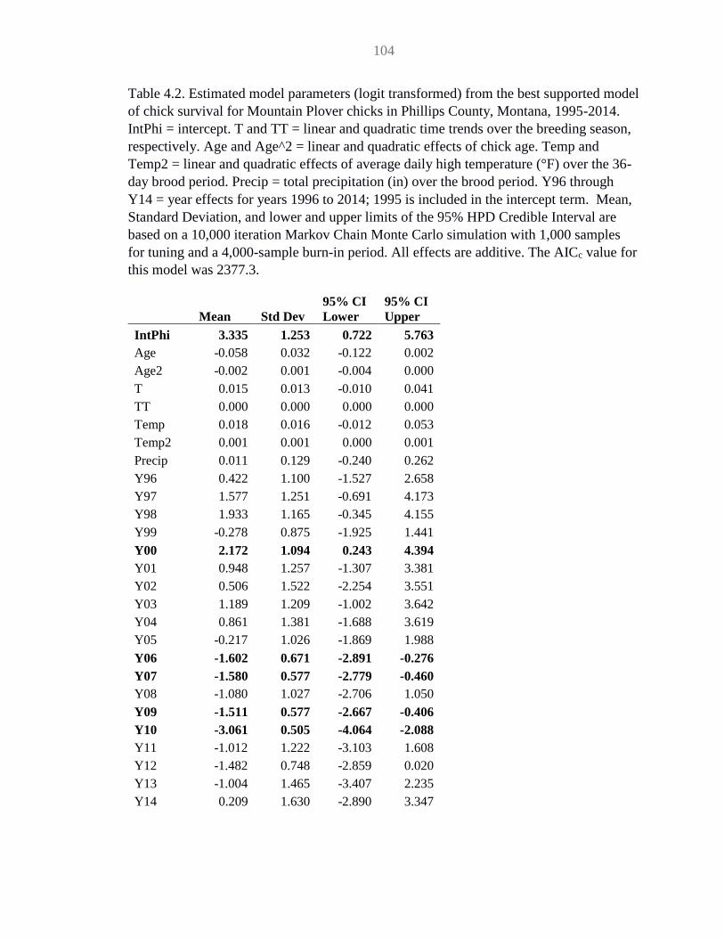
104

Table 4.2. Estimated model parameters (logit transformed) from the best supported model

of chick survival for Mountain Plover chicks in Phillips County, Montana, 1995-2014.

IntPhi = intercept. T and TT = linear and quadratic time trends over the breeding season,

respectively. Age and Age^2 = linear and quadratic effects of chick age. Temp and

Temp2 = linear and quadratic effects of average daily high temperature (°F) over the 36-

day brood period. Precip = total precipitation (in) over the brood period. Y96 through

Y14 = year effects for years 1996 to 2014; 1995 is included in the intercept term. Mean,

Standard Deviation, and lower and upper limits of the 95% HPD Credible Interval are

based on a 10,000 iteration Markov Chain Monte Carlo simulation with 1,000 samples

for tuning and a 4,000-sample burn-in period. All effects are additive. The AICc value for

this model was 2377.3.

Mean Std Dev

95% CI

Lower

95% CI

Upper

IntPhi 3.335 1.253 0.722 5.763

Age -0.058 0.032 -0.122 0.002

Age2 -0.002 0.001 -0.004 0.000

T 0.015 0.013 -0.010 0.041

TT 0.000 0.000 0.000 0.000

Temp 0.018 0.016 -0.012 0.053

Temp2 0.001 0.001 0.000 0.001

Precip 0.011 0.129 -0.240 0.262

Y96 0.422 1.100 -1.527 2.658

Y97 1.577 1.251 -0.691 4.173

Y98 1.933 1.165 -0.345 4.155

Y99 -0.278 0.875 -1.925 1.441

Y00 2.172 1.094 0.243 4.394

Y01 0.948 1.257 -1.307 3.381

Y02 0.506 1.522 -2.254 3.551

Y03 1.189 1.209 -1.002 3.642

Y04 0.861 1.381 -1.688 3.619

Y05 -0.217 1.026 -1.869 1.988

Y06 -1.602 0.671 -2.891 -0.276

Y07 -1.580 0.577 -2.779 -0.460

Y08 -1.080 1.027 -2.706 1.050

Y09 -1.511 0.577 -2.667 -0.406

Y10 -3.061 0.505 -4.064 -2.088

Y11 -1.012 1.222 -3.103 1.608

Y12 -1.482 0.748 -2.859 0.020

Y13 -1.004 1.465 -3.407 2.235

Y14 0.209 1.630 -2.890 3.347

105

Figure 4.1. Daily and cumulative Mountain Plover chick survival probability over the

brood period generated using mean covariate values, Phillips County, Montana, 1995-

2014. Error bars are based on 95% HPD credible intervals. Cumulative survival is the

product of all previous values of daily survival.

0.50

0.55

0.60

0.65

0.70

0.75

0.80

0.85

0.90

0.95

1.00

0 4 8 12 16 20 24 28 32 36

Su

rviv

al P

rob

abil

ity

Chick Age (days)

Daily

Cumulative

106

Figure 4.2. Periods of monitoring for Mountain Plover broods in Phillips County,

Montana, 1996-2012. Only broods that had ≥2 resightings with 1 or more chicks are

included (n = 80). Light bars represent the 36-day interval between estimated hatch and

fledging dates. Dark bars represent the interval between the first and last resighting of ≥1

chick for each brood.

10 30 50 70 90 110

2012

2011

2010200920082007

2006

200520042003

2001

2000

1999

1998

19971996

Day of Season

Yea

r

107

CHAPTER 5

GENERAL CONCLUSIONS

This project’s stated goals were 1) to investigate and quantify the factors

influencing nest detection probability; 2) to characterize the spatial patterning of

Mountain Plover nests on prairie dog colonies in Phillips County, Montana and attempt to

link spatial characteristics of nest sites to nest survival; and 3) to model Mountain Plover

chick survival and its influences using resighting data on marked adults in the same area.

I demonstrated the use of a Huggins Closed Capture model for modeling nest

detection probability and showed that nest detection probability in the Mountain Plover is

primarily influenced by nest initiation date, day of season, nest age, prairie dog colony

size, observer skill level, nest fate, and year. Single-visit nest detection probability was

highly variable and ranged from <0.10 to >0.80, clearly demonstrating the utility of a

model-based approach that accounts for individual heterogeneity and temporal variation

at multiple time scales. I also demonstrated how cumulative detection probability

increases over multiple surveys and increases more quickly with more frequent surveys,

with implications for study design and the allocation of survey effort. These findings

should prove useful to others who are interested in (1) exploring factors affecting nest

detection probability in general, or (2) using information about imperfect nest detection

in models predicting a species’ population change.

I analyzed the spatial patterning of Mountain Plover nests on prairie dog colonies

in Montana and provided evidence that Mountain Plover nests are not placed at random

but rather show inhibition at small scales in response to proximity to conspecifics. I

108

attempted to incorporate the number and proximity of neighboring nests and the

placement of plover nests within prairie dog colonies into estimates of nest survival but

found no significant effects of these covariates. This suggests that nest placement is not a

strategy to optimize nest survival but is likely a territorial response to conspecifics. These

findings (1) build on our general understanding of nest spacing patterns in a non-colonial

nesting bird, and (2) provide detailed information specific to the plover, which may be

useful for prairie dog colony management to benefit this species.

Finally, I used a long-term data set on banding and resighting of adult Mountain

Plovers to model the survival of unmarked dependent chicks from hatch until fledging.

The best model included linear and quadratic trends across the breeding season, linear

and quadratic effects of chick age and average daily high temperature, precipitation, and

year effects, but the effects of these covariates were not well estimated. I tentatively

concluded that chick survival was influenced by chick age, day of season, temperature,

and year, but that the data set did not include the necessary information to estimate these

effects with precision or generate useful estimates of daily survival for specific chicks.

Together these findings represent an advancement in our understanding of avian

breeding ecology in general and the ecology of the Mountain Plover in particular. I have

provided a broadly applicable approach to estimating nest detection probability in birds

and potentially other taxa, which will improve estimates of breeding activity and enable

more effective management of species of concern. I have provided the first rigorous

characterization of the spatial patterning of Mountain Plover nests, giving us a better

understanding of the species’ breeding habitat requirements, and provided evidence that

dispersion or clustering of nests is not a major factor in nest survival in this species.

109

Finally, I have provided weak evidence for several influences on Mountain Plover chick

survival and shown the limitations of using general-purpose data to estimate this

parameter.

breeding ecology of the mountain plover (charadrius

Documents