bregman voronoi diagrams: properties, algorithms and

HAL Id: inria-00137865https://hal.inria.fr/inria-00137865v2

Submitted on 19 Apr 2007

HAL is a multi-disciplinary open accessarchive for the deposit and dissemination of sci-entific research documents, whether they are pub-lished or not. The documents may come fromteaching and research institutions in France orabroad, or from public or private research centers.

L’archive ouverte pluridisciplinaire HAL, estdestinée au dépôt et à la diffusion de documentsscientifiques de niveau recherche, publiés ou non,émanant des établissements d’enseignement et derecherche français ou étrangers, des laboratoirespublics ou privés.

Bregman Voronoi Diagrams: Properties, Algorithms andApplications

Jean-Daniel Boissonnat, Frank Nielsen, Richard Nock

To cite this version:Jean-Daniel Boissonnat, Frank Nielsen, Richard Nock. Bregman Voronoi Diagrams: Properties, Al-gorithms and Applications. [Research Report] RR-6154, INRIA. 2007, pp.48. �inria-00137865v2�

https://hal.inria.fr/inria-00137865v2

https://hal.archives-ouvertes.fr

appor t de r ech er ch e

ISS

N02

49-6

399

ISR

NIN

RIA

/RR

--61

54--

FR

+E

NG

Thème SYM

INSTITUT NATIONAL DE RECHERCHE EN INFORMATIQUE ET EN AUTOMATIQUE

Bregman Voronoi Diagrams: Properties, Algorithmsand Applications

Frank Nielsen — Jean-Daniel Boissonnat — Richard Nock

N° 6154

Mars 2007

Unité de recherche INRIA Sophia Antipolis2004, route des Lucioles, BP 93, 06902 Sophia Antipolis Cedex (France)

Téléphone : +33 4 92 38 77 77 — Télécopie : +33 4 92 38 77 65

Bregman Voronoi Diagrams: Properties, Algorithmsand Applications

Frank Nielsen∗ , Jean-Daniel Boissonnat† , Richard Nock‡

Theme SYM — Systemes symboliquesProjet Geometrica

Rapport de recherche n° 6154 — Mars 2007 — 48 pages

Abstract: The Voronoi diagram of a finite set of objects is a fundamental geometricstructure that subdivides the embedding space into regions, each region consisting of thepoints that are closer to a given object than to the others. We may define many variantsof Voronoi diagrams depending on the class of objects, the distance functions and the em-bedding space. In this paper, we investigate a framework for defining and building Voronoidiagrams for a broad class of distance functions called Bregman divergences. Bregman di-vergences include not only the traditional (squared) Euclidean distance but also variousdivergence measures based on entropic functions. Accordingly, Bregman Voronoi diagramsallow to define information-theoretic Voronoi diagrams in statistical parametric spaces basedon the relative entropy of distributions. We define several types of Bregman diagrams, es-tablish correspondences between those diagrams (using the Legendre transformation), andshow how to compute them efficiently. We also introduce extensions of these diagrams, e.g.k-order and k-bag Bregman Voronoi diagrams, and introduce Bregman triangulations of aset of points and their connexion with Bregman Voronoi diagrams. We show that thesetriangulations capture many of the properties of the celebrated Delaunay triangulation. Fi-nally, we give some applications of Bregman Voronoi diagrams which are of interest in thecontext of computational geometry and machine learning.

Key-words: Computational Information Geometry, Voronoi diagram, Delaunay trian-gulation, Bregman divergence, Quantification, Sampling, Clustering

A preliminary version appeared in the 18th ACM-SIAM Symposium on Discrete Algorithms (SODA),pp. 746-755, 2007. Related materials are available online at http://www.csl.sony.co.jp/person/nielsen/

BregmanVoronoi/

∗ Sony Computer Science Laboratories Inc., Fundamental Research Laboratory, Japan.† INRIA Sophia-Antipolis, GEOMETRICA, France.‡ Universite Antilles-Guyane, CEREGMIA, France.

http://www.csl.sony.co.jp/person/nielsen/BregmanVoronoi/

http://www.csl.sony.co.jp/person/nielsen/BregmanVoronoi/

Diagrammes de Bregman-Voronoi : Proprietes,Algorithmes et Applications

Resume : Les diagrammes de Voronoı sont des structures geometriques fondamentales quiassocient a un ensemble fini d’objets une partition de l’espace en regions, chaque region etantconstituee des points qui sont plus plus proches d’un objet que des autres. On peut definirbeaucoup de variantes de ces diagrammes selon le choix qui est fait de la classe des objetsconsideres, de la metrique utilisee et de l’espace ambiant. Dans cet article, on etudie les dia-grammes de Voronoı associes a une large classe de fonctions distance appelees les divergencesde Bregman. Les divergences de Bregman incluent la distance euclidienne (au carre) et ausside nombreuses divergences utilisees en theorie de l’information et en statistiques. Les dia-grammes de Bregman-Voronoı permettent de definir des diagrammes informationnels dansdes espaces statistiques parametriques ou les objets sont des distributions de probabiliteset la distance mesure l’entropie relative entre deux distributions. On definit plusieurs typesde diagrammes de Bregman-Voronoı, relies par la transformee de Legendre, et on montrecomment calculer ces diagrammes efficacement. On introduit differentes extensions de cesdiagrammes et des structures duales, les triangulations de Bregman, qui possedent beaucoupdes proprietes des triangulations de Delaunay. Pour finir, nous presentons des applicationsen geometrie algorithmique et en apprentissage statistique.

Mots-cles : Geometrie de l’information, geometrie algorithmique, diagrammes de Vo-ronoı, divergence de Bregman, quantification, echantillonnage, classification

Bregman Voronoi Diagrams: Properties, Algorithms and Applications 3

1 Introduction and prior work

The Voronoi diagram vor(S) of a set of n points S = {p1, ...,pn} of the d-dimensionalEuclidean space Rd is defined as the cell complex whose d-cells are the Voronoi regions{vor(pi)}i∈{1,..,n} where vor(pi) is the set of points of Rd closer to pi than to any otherpoint of S with respect to a distance function δ:

vor(pi)def= {x ∈ Rd | δ(pi,x) ≤ δ(pj ,x) ∀ pj ∈ S}.

Points {pi}i are called the Voronoi sites or Voronoi generators. Since its inception indisguise by Descartes in the 17th century [5], Voronoi diagrams have found a broad spectrumof applications in science. Computational geometers have focused at first on EuclideanVoronoi diagrams [5] by considering the case where δ(x,y) is the Euclidean distance ||x −y|| =

√∑di=1(xi − yi)2. Voronoi diagrams have been later on defined and studied for other

distance functions, most notably the L1 distance ||x − y||1 =∑d

i=1 |xi − yi| (Manhattandistance) and the L∞ distance ||x − y||∞ = maxi∈{1,...,d} |xi − yi| [10, 5]. Klein furtherpresented an abstract framework for describing and computing the fundamental structuresof abstract Voronoi diagrams [26, 11].

In artificial intelligence, machine learning techniques also rely on geometric conceptsfor building classifiers in supervised problems (e.g., linear separators, oblique decision trees,etc.) or clustering data in unsupervised settings (e.g., k-means, support vector clustering [2],etc.). However, the considered data sets S and their underlying spaces X are usually notmetric spaces. The notion of distance between two elements of X needs to be replaced by apseudo-distance that is not necessarily symmetric and may not satisfy the triangle inequality.Such a pseudo-distance is also referred to as distortion, (dis)similarity or divergence inthe literature. For example, in parametric statistical spaces X , a vector point represent adistribution and its coordinates store the parameters of the associated distribution. A notionof “distance” between two such points is then needed to represent the divergence betweenthe corresponding distributions.

Very few works have tackled an in-depth study of Voronoi diagrams and their applica-tions for such a kind of statistical spaces. This is all the more important even for ordinaryVoronoi diagrams as Euclidean point location of sites are usually observed in noisy environ-ments (e.g., imprecise point measures in computer vision experiments), and “noise” is oftenmodeled by means of Normal distributions (so-called “Gaussian noise”). To the best of ourknowledge, statistical Voronoi diagrams have only been considered in a 4-page short pa-per of Onishi and Imai [34] which relies on Kullback-Leibler divergence of dD multivariatenormal distributions to study combinatorics of their Voronoi diagrams, and subsequentlyin a 2-page video paper of Sadakane et al. [40] which defines the divergence implied by aconvex function and its conjugate, and present the Voronoi diagram with flavors of infor-mation geometry [1] (see also [35] and related short communications [25, 24]). Our studyof Bregman Voronoi diagrams generalizes and subsumes these preliminary studies using aneasier concept of divergence: Bregman divergences [12, 6] that do not rely explicitly on

RR n° 6154

4 Nielsen & Boissonnat & Nock

p1

p2

p3

p4

p5

p6

p7

p6

Vor(p6)

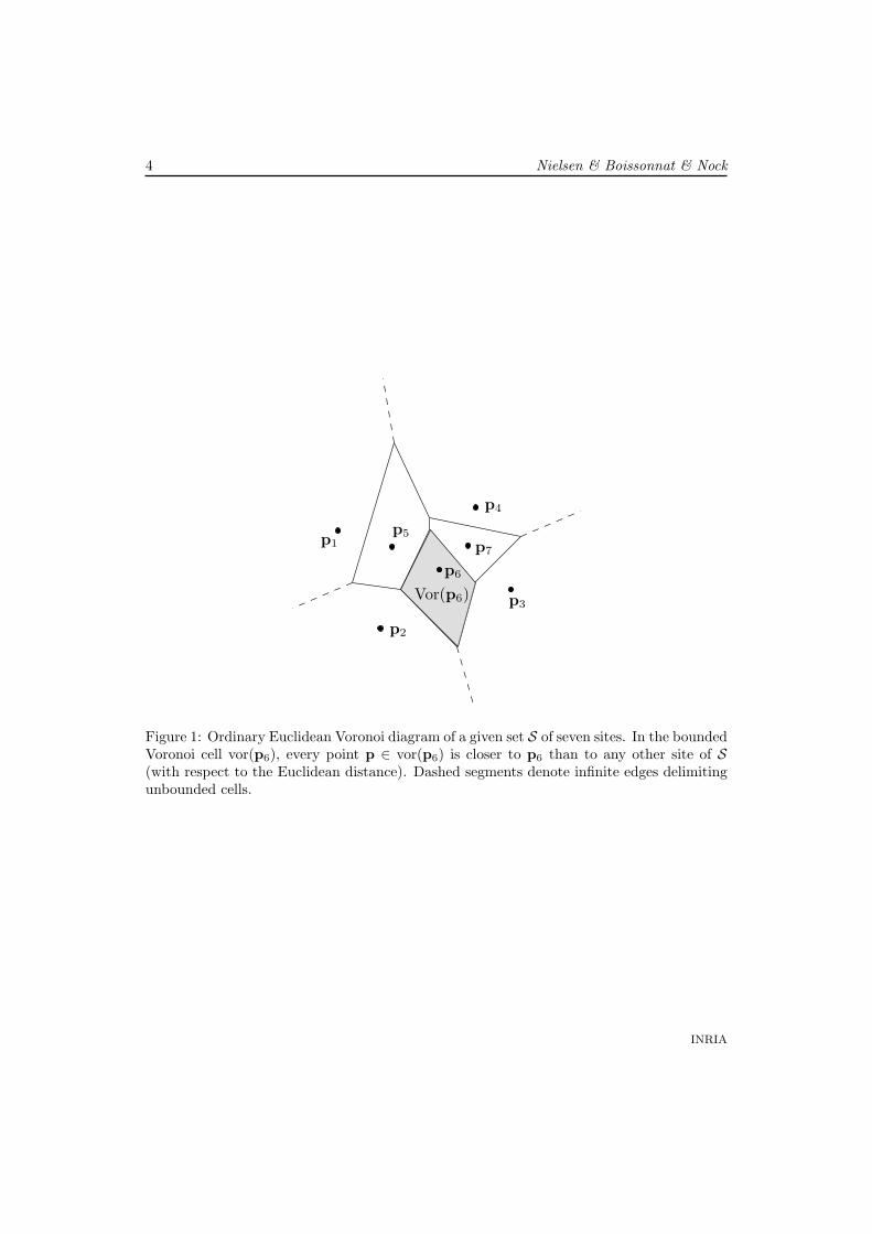
Figure 1: Ordinary Euclidean Voronoi diagram of a given set S of seven sites. In the boundedVoronoi cell vor(p6), every point p ∈ vor(p6) is closer to p6 than to any other site of S(with respect to the Euclidean distance). Dashed segments denote infinite edges delimitingunbounded cells.

INRIA


convex conjugates. Bregman divergences encapsulate the squared Euclidean distance andmany widely used divergences, e.g. the Kullback-Leibler divergence. It should be noticedhowever that other divergences have been defined and studied in the context of Riemanniangeometry [1]. Sacrifying for some generality, while not very restrictive in practice, allows amuch simpler treatment and our study of Bregman divergences is elementary and does notrely on Riemannian geometry.

In this paper, we give a thorough treatment of Bregman Voronoi diagrams which el-egantly unifies the ordinary Euclidean Voronoi diagram and statistical Voronoi diagrams.Our contributions are summarized as follows:

� Since Bregman divergences are not symmetric, we define two types of Bregman Voronoidiagrams. One is an affine diagram with convex polyhedral cells while the otherone is curved. The cells of those two diagrams are in 1-1 correspondence throughthe Legendre transformation. We also introduce a third-type symmetrized BregmanVoronoi diagram.

� We present a simple way to compute the Bregman Voronoi diagram of a set of pointsby lifting the points in a higher dimensional space using an extra dimension. Thismapping leads also to combinatorial bounds on the size of these diagrams. We alsodefine weighted Bregman Voronoi diagrams and show that the class of these diagrams isidentical to the class of affine (or power) diagrams. Special cases of weighted BregmanVoronoi diagrams are the k-order and k-bag Bregman Voronoi diagrams.

� We define two triangulations of a set of points. The first one captures some of themost important properties of the well-known Delaunay triangulation. The secondtriangulation is called a geodesic Bregman triangulation since its edges are geodesicarcs. Differently from the first triangulation, this triangulation is the geometric dualof the first-type Bregman Voronoi diagram of its vertices.

� We give a few applications of Bregman Voronoi diagrams which are of interest in thecontext of computational geometry and machine learning.

The outline of the paper is as follows: In Section 2, we define Bregman divergencesand recall some of their basic properties. In Section 3, we study the geometry of Bregmanspaces and characterize bisectors, balls and geodesics. Section 4 is devoted to BregmanVoronoi diagrams and Section 5 to Bregman triangulations. In Section 6, we select of fewapplications of interest in computational geometry and machine learning. Finally, Section 7concludes the paper and mention further ongoing investigations.

Notations. In the whole paper, X denotes an open convex domain of Rd and F : X 7→ Ra strictly convex and differentiable function. F denotes the graph of F , i.e. the set of points(x, z) ∈ X × R where z = F (x). We write x for the point (x, F (x)) ∈ F . ∇F , ∇2F and∇−1F denote respectively the gradient, the Hessian and the inverse gradient of F .

RR n° 6154


2 Bregman divergences

In this section, we recall the definition of Bregman1 divergences and some of their mainproperties (§2.1). We show that the notion of Bregman divergence encapsulates the squaredEuclidean distance as well as several well-known information-theoretic divergences. Weintroduce the notion of dual divergences (§2.2) and show how this comes in handy forsymmetrizing Bregman divergences (§2.3). Finally, we prove that the Kullback-Leibler di-vergence of distributions that belong to the exponential family of distributions can be viewedas a Bregman divergence (§2.4).

2.1 Definition and basic properties

For any two points p and q of X ⊆ Rd, the Bregman divergence2 DF (·||·) : X 7→ R of p toq associated to a strictly convex and differentiable function F (called the generator functionof the divergence) is defined as

DF (p||q) def= F (p)− F (q)− 〈∇F (q),p− q〉, (1)

where ∇F = [ ∂F∂x1

... ∂F∂xd

]T denotes the gradient operator, and 〈p,q〉 the inner (or dot)

product:∑d

i=1 piqi.Informally speaking, Bregman divergence DF is the tail of the Taylor expansion of F .

See [16] for an axiomatic characterization of Bregman divergences as “permissible” diver-gences.

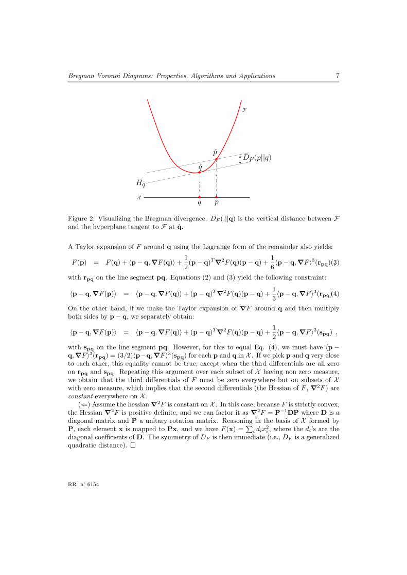
Lemma 1 The Bregman divergence DF (p||q) is geometrically measured as the vertical dis-tance between p and the hyperplane Hq tangent to F at point q: DF (p||q) = F (p)−Hq(p).

Proof: The tangent hyperplane to hypersurface F : z = F (x) at point q is Hq : z =F (q) + 〈∇F (q),x− q〉. It follows that DF (p||q) = F (p)−Hq(p) (see Figure 2). �

We now give some basic properties of Bregman divergences. The first property seems tobe new. The others are well known. First, observe that, for most functions F , the associatedBregman divergence is not symmetric, i.e. DF (p||q) 6= DF (q||p) (the symbol || is put toemphasize this point, as is standard in information theory). The following lemma provesthis claim.

Lemma 2 Let F be properly defined for DF to exist. Then DF is symmetric if and only ifthe Hessian ∇2F is constant on X .

Proof: (⇒) From Eq. 1, the symmetry DF (p||q) = DF (q||p) yields:

F (p) = F (q) +12〈p− q,∇F (q) + ∇F (p)〉 . (2)

1Lev M. Bregman historically pioneered this notion in the seminal work [12] on minimization of a convexobjective function under linear constraints. See http://www.math.bgu.ac.il/serv/segel/bregman.html.We gratefully acknowledge him for sending us this historical paper.

2See Java� applet at http://www.csl.sony.co.jp/person/nielsen/BregmanDivergence/

INRIA

http://www.math.bgu.ac.il/serv/segel/bregman.html

http://www.csl.sony.co.jp/person/nielsen/BregmanDivergence/


F

Xpq

p

q

Hq

DF (p||q)

Figure 2: Visualizing the Bregman divergence. DF (.||q) is the vertical distance between Fand the hyperplane tangent to F at q.

A Taylor expansion of F around q using the Lagrange form of the remainder also yields:

F (p) = F (q) + 〈p− q,∇F (q)〉+12(p− q)T ∇2F (q)(p− q) +

16〈p− q,∇F 〉3(rpq) ,(3)

with rpq on the line segment pq. Equations (2) and (3) yield the following constraint:

〈p− q,∇F (p)〉 = 〈p− q,∇F (q)〉+ (p− q)T ∇2F (q)(p− q) +13〈p− q,∇F 〉3(rpq) .(4)

On the other hand, if we make the Taylor expansion of ∇F around q and then multiplyboth sides by p− q, we separately obtain:

〈p− q,∇F (p)〉 = 〈p− q,∇F (q)〉+ (p− q)T ∇2F (q)(p− q) +12〈p− q,∇F 〉3(spq) ,

with spq on the line segment pq. However, for this to equal Eq. (4), we must have 〈p −q,∇F 〉3(rpq) = (3/2)〈p−q,∇F 〉3(spq) for each p and q in X . If we pick p and q very closeto each other, this equality cannot be true, except when the third differentials are all zeroon rpq and spq. Repeating this argument over each subset of X having non zero measure,we obtain that the third differentials of F must be zero everywhere but on subsets of Xwith zero measure, which implies that the second differentials (the Hessian of F , ∇2F ) areconstant everywhere on X .

(⇐) Assume the hessian ∇2F is constant on X . In this case, because F is strictly convex,the Hessian ∇2F is positive definite, and we can factor it as ∇2F = P−1DP where D is adiagonal matrix and P a unitary rotation matrix. Reasoning in the basis of X formed byP, each element x is mapped to Px, and we have F (x) =

∑i dix

2i , where the di’s are the

diagonal coefficients of D. The symmetry of DF is then immediate (i.e., DF is a generalizedquadratic distance). �

RR n° 6154


Property 1 (Non-negativity) The strict convexity of generator function F implies that,for any p and q in X , DF (p||q) ≥ 0, with DF (p||q) = 0 if and only if p = q.

Property 2 (Convexity) Function DF (p||q) is convex in its first argument p but notnecessarily in its second argument q.

Bregman divergences can easily be constructed from simpler ones. For instance, mul-tivariate Bregman divergences DF can be created from univariate generator functionscoordinate-wise as F (x) =

∑di=1 fi(xi) with ∇F = [ df1

dx1... dfd

dxd]T .

Because positive linear combinations of strictly convex and differentiable functions arestrictly convex and differentiable functions, new generator functions (and correspondingBregman divergences) can also be built as positive linear combinations of elementary gen-erator functions. This is an important property as it allows to handle mixed data sets ofheterogenous types in a unified framework.

Property 3 (Linearity) Bregman divergence is a linear operator, i.e., for any two strictlyconvex and differentiable functions F1 and F2 defined on X and for any λ ≥ 0:

DF1+λF2(p||q) = DF1(p||q) + λDF2(p||q).

Property 4 (Invariance under linear transforms) G(x) = F (x) + 〈a,x〉+ b, with a ∈Rd and b ∈ R, is a strictly convex and differentiable function on X , and DG(p||q) =DF (p||q).

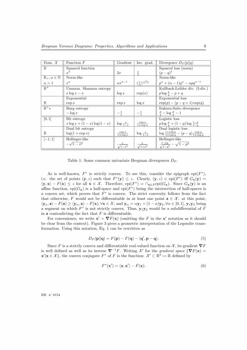
Examples of Bregman divergences are the squared Euclidean distance (obtained forF (x) = ‖x‖2 and the generalized quadratic distance function F (x) = xT Qx where Q isa positive definite matrix. When Q is taken to be the inverse of the variance-covariancematrix, DF is the Mahalanobis distance, extensively used in computer vision. More impor-tantly, the notion of Bregman divergence encapsulates various information measures basedon entropic functions such as the Kullback-Leibler divergence based on the (unnormalized)Shannon entropy, or the Itakura-Saito divergence based on Burg entropy (commonly usedin sound processing). Table 1 lists the main univariate Bregman divergences.

2.2 Legendre duality

We now turn to an essential notion of convex analysis: Legendre transform that will allowus to associate to any Bregman divergence a dual Bregman divergence.

Let F be a strictly convex and differentiable real-valued function on X . The Legendretransformation makes use of the duality relationship between points and lines to associateto F a convex conjugate function F ∗ : Rd 7→ R given by [38]:

F ∗(y) = supx∈X

{〈y,x〉 − F (x)}.

The supremum is reached at the unique point where the gradient of G(x) = 〈y,x〉−F (x)vanishes or, equivalently, when y = ∇F (x).

INRIA


Dom. X Function F Gradient Inv. grad. Divergence DF (p||q)R Squared function Squared loss (norm)

x2 2x x2

(p− q)2

R+, α ∈ N Norm-like Norm-like

α > 1 xα αxα−1 ( xα)

1α−1 pα + (α− 1)qα − αpqα−1

R+ Unnorm. Shannon entropy Kullback-Leibler div. (I-div.)x log x− x log x exp(x) p log p

q− p + q

Exponential Exponential lossR exp x exp x log x exp(p)− (p− q + 1) exp(q)

R+∗ Burg entropy Itakura-Saito divergence− log x − 1

x− 1

xpq− log p

q− 1

[0, 1] Bit entropy Logistic lossx log x + (1− x) log(1− x) log x

1−xexp x

1+exp xp log p

q+ (1− p) log 1−p

1−q

Dual bit entropy Dual logistic lossR log(1 + exp x) exp x

1+exp xlog x

1−xlog 1+exp p

1+exp q− (p− q) exp q

1+exp q

[−1, 1] Hellinger-like Hellinger-like

−√

1− x2 x√1−x2

x√1+x2

1−pq√1−q2

−p

1− p2

Table 1: Some common univariate Bregman divergences DF .

As is well-known, F ∗ is strictly convex. To see this, consider the epigraph epi(F ∗),i.e. the set of points (y, z) such that F ∗(y) ≤ z. Clearly, (y, z) ∈ epi(F ∗) iff Gx(y) =〈y,x〉 − F (x) ≤ z for all x ∈ X . Therefore, epi(F ∗) = ∩x∈X epi(Gx). Since Gx(y) is anaffine function, epi(Gx) is a half-space and epi(F ∗) being the intersection of half-spaces isa convex set, which proves that F ∗ is convex. The strict convexity follows from the factthat otherwise, F would not be differentiable in at least one point z ∈ X : at this point,〈yα, z〉 − F (z) ≥ 〈yα,x〉 − F (x),∀x ∈ X , and yα = αy1 + (1− α)y2,∀α ∈ [0, 1], y1y2 beinga segment on which F ∗ is not strictly convex. Thus, y1y2 would be a subdifferential of Fin z contradicting the fact that F is differentiable.

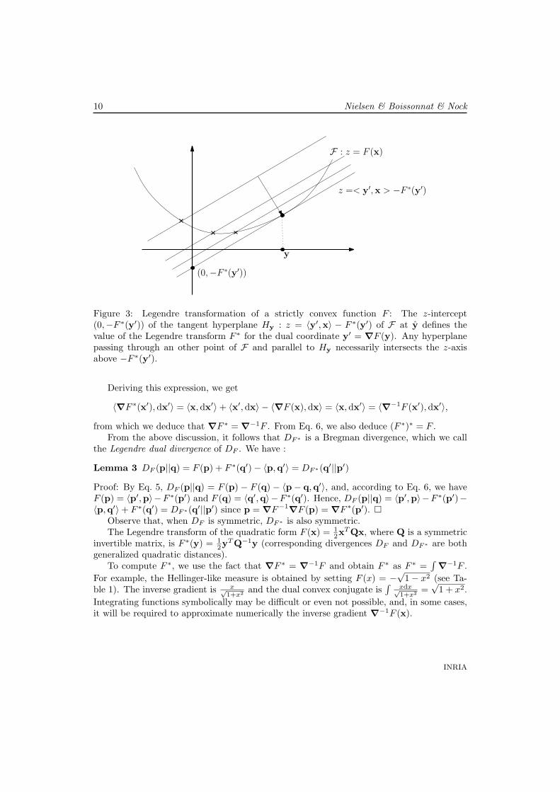
For convenience, we write x′ = ∇F (x) (omitting the F in the x′ notation as it shouldbe clear from the context). Figure 3 gives a geometric interpretation of the Legendre trans-formation. Using this notation, Eq. 1 can be rewritten as

DF (p||q) = F (p)− F (q)− 〈q′,p− q〉. (5)

Since F is a strictly convex and differentiable real-valued function on X , its gradient ∇Fis well defined as well as its inverse ∇−1F . Writing X ′ for the gradient space {∇F (x) =x′|x ∈ X}, the convex conjugate F ∗ of F is the function: X ′ ⊂ Rd 7→ R defined by

F ∗(x′) = 〈x,x′〉 − F (x). (6)

RR n° 6154


F : z = F (x)

(0,−F ∗(y′))

y

z =< y′,x > −F ∗(y′)

Figure 3: Legendre transformation of a strictly convex function F : The z-intercept(0,−F ∗(y′)) of the tangent hyperplane Hy : z = 〈y′,x〉 − F ∗(y′) of F at y defines thevalue of the Legendre transform F ∗ for the dual coordinate y′ = ∇F (y). Any hyperplanepassing through an other point of F and parallel to Hy necessarily intersects the z-axisabove −F ∗(y′).

Deriving this expression, we get

〈∇F ∗(x′),dx′〉 = 〈x,dx′〉+ 〈x′,dx〉 − 〈∇F (x),dx〉 = 〈x,dx′〉 = 〈∇−1F (x′),dx′〉,

from which we deduce that ∇F ∗ = ∇−1F . From Eq. 6, we also deduce (F ∗)∗ = F .From the above discussion, it follows that DF∗ is a Bregman divergence, which we call

the Legendre dual divergence of DF . We have :

Lemma 3 DF (p||q) = F (p) + F ∗(q′)− 〈p,q′〉 = DF∗(q′||p′)

Proof: By Eq. 5, DF (p||q) = F (p) − F (q) − 〈p− q,q′〉, and, according to Eq. 6, we haveF (p) = 〈p′,p〉−F ∗(p′) and F (q) = 〈q′,q〉−F ∗(q′). Hence, DF (p||q) = 〈p′,p〉−F ∗(p′)−〈p,q′〉+ F ∗(q′) = DF∗(q′||p′) since p = ∇F−1∇F (p) = ∇F ∗(p′). �

Observe that, when DF is symmetric, DF∗ is also symmetric.The Legendre transform of the quadratic form F (x) = 1

2xT Qx, where Q is a symmetric

invertible matrix, is F ∗(y) = 12y

T Q−1y (corresponding divergences DF and DF∗ are bothgeneralized quadratic distances).

To compute F ∗, we use the fact that ∇F ∗ = ∇−1F and obtain F ∗ as F ∗ =∫

∇−1F .For example, the Hellinger-like measure is obtained by setting F (x) = −

√1− x2 (see Ta-

ble 1). The inverse gradient is x√1+x2 and the dual convex conjugate is

∫xdx√1+x2 =

√1 + x2.

Integrating functions symbolically may be difficult or even not possible, and, in some cases,it will be required to approximate numerically the inverse gradient ∇−1F (x).

INRIA


Let us consider the univariate generator functions defining the divergences of Table 1.Both the squared function F (x) = x2 and Burg entropy F (x) = − log x are self-dual, i.e.F = F ∗. This is easily seen by noticing that the gradient and inverse gradient are identical(up to some constant factor).

For the exponential function F (x) = exp x, we have F ∗(y) = y log y−y (the unnormalizedShannon entropy) and for the dual bit entropy F (x) = log(1 + expx), we have F ∗(y) =y log y

1−y + log(1 − y), the bit entropy. Note that the bit entropy function is a particularBregman generator satisfying F (x) = F (1− x).

2.3 Symmetrized Bregman divergences

For non-symmetric d-variate Bregman divergences DF , we define the symmetrized divergence

SF (p,q) = SF (q,p) =12

(DF (p||q) + DF (q||p)) =12〈p− q,p′ − q′〉.

An example of such a symmetrized divergence is the symmetric Kullback-Leibler diver-gence (SKL) widely used in computer vision and sound processing (see for example [29]).

A key observation is to note that the divergence SF between two points of X can be mea-sured as a divergence in X ×X ′ ⊂ R2d. More precisely, let x = [x x′]T be the 2d-dimensionalvector obtained by stacking the coordinates of x on top of those of x′, the gradient of F atx. We have :

Theorem 1 SF (p,q) = 12DF (p||q) where F (x) = F (x) + F ∗(x′) and DF is the Bregman

divergence defined over X × X ′ ⊂ R2d for the generator function F .

Proof: Using Lemma 3, we have

SF (p,q) =12

(DF (p||q) + DF (q||p)) =12

(DF (p||q) + DF∗(p′||q′)) =12DF (p||q)

�It should be noted that x lies on the d-manifold X = {[x x′]T | x ∈ Rd} of R2d. Note

also that SF (p,q) is symmetric but not a Bregman divergence in general while DF is a nonsymmetric Bregman divergence in X × X ′.

2.4 Exponential families

2.4.1 Parametric statistical spaces and exponential families

A statistical space X is an abstract space where coordinates of vector points θ ∈ X encodethe parameters of statistical distributions. The dimension d = dimX of the statistical spacecoincides with the finite number of free parameters of the distribution laws. For example,the space X = {[µ σ]T | (µ, σ) ∈ R × R+

∗ } of univariate normal distributions N (µ, σ) isa 2D parametric statistical space, extensively studied in information geometry [1] under

RR n° 6154


the auspices of differential geometry. A prominent class of distribution families called theexponential families EF [1] admits the same canonical probability distribution function

p(x|θ) def= exp{〈θ, f(x)〉 − F (θ) + C(x)}, (7)

where f(x) denotes the sufficient statistics and θ ∈ X represents the natural parameters.Space X is thus called the natural parameter space and, since log

∫x

p(x|θ)dx = log 1 = 0, wehave F (θ) = log

∫x

exp{〈θ, f(x)〉 + C(x)}dx. F is called the cumulant function or the log-partition function. F fully characterizes the exponential family EF while term C(x) ensuresdensity normalization. (That is, p(x|θ) is indeed a probability density function satisfying∫

xp(x|θ)dx = 1.)When the components of the sufficient statistics are affinely independent, this canonical

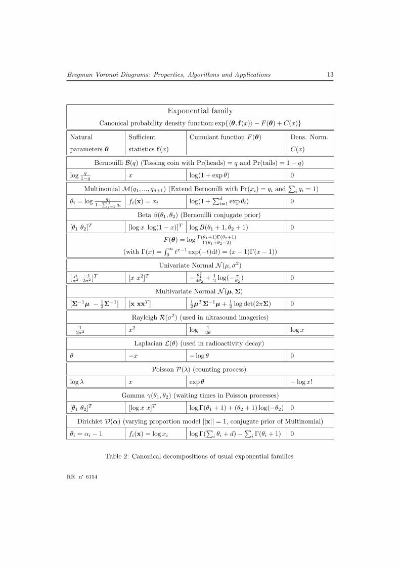
representation is said to be minimal, and the family EF is called a full exponential familyof order d = dimX . Moreover, we consider regular exponential families EF that have theirsupport domains topologically open. Regular exponential families include many famousdistribution laws such as Bernoulli (multinomial), Normal (univariate, multivariate and rec-tified), Poisson, Laplacian, negative binomial, Rayleigh, Wishart, Dirichlet, and Gammadistributions. Table 2 summarizes the various relevant parts of the canonical decomposi-tions of some of these usual statistical distributions. Observe that the product of any twodistributions of the same exponential family is another exponential family distribution thatmay not have anymore a nice parametric form (except for products of normal distributionpdfs that yield again normal distribution pdfs). Thus exponential families provide a unifiedtreatment framework of common distributions. Note, however, that the uniform distributiondoes not belong to the exponential families.

2.4.2 Kullback-Leibler divergence of exponential families

In such statistical spaces X , a basic primitive is to measure the distortion between any twodistributions. The Kullback-Leibler divergence (also called relative entropy or informationdivergence, I-divergence) is a standard information-theoretic measure between two statis-tical distributions d1 and d2 defined as KL(d1||d2)

def=∫

xd1(x) log d1(x)

d2(x)dx. This statisticalmeasure is not symmetric nor does the triangle inequality holds.

The link with Bregman divergences comes from the remarkable property that theKullback-Leibler divergence of any two distributions of the same exponential family withrespective natural parameters θp and θq is obtained from the Bregman divergence in-duced by the cumulant function of that family by swapping arguments. By a slightabuse of notations, we denote by KL(θp||θq) the oriented Kullback-Leibler divergence be-tween the probability density functions defined by the respective natural parameters, i.e.KL(θp||θq)

def=∫

xp(x|θp) log p(x|θp)

p(x|θq)dx. The following theorem is the extension to the con-tinuous case of a result mentioned in [6].

INRIA


Exponential family

Canonical probability density function: exp{〈θ, f(x)〉 − F (θ) + C(x)}

Natural Sufficient Cumulant function F (θ) Dens. Norm.

parameters θ statistics f(x) C(x)

Bernouilli B(q) (Tossing coin with Pr(heads) = q and Pr(tails) = 1− q)

log q1−q x log(1 + exp θ) 0

Multinomial M(q1, ..., qd+1) (Extend Bernouilli with Pr(xi) = qi and∑

i qi = 1)

θi = log qi

1−Pd

j=1 qifi(x) = xi log(1 +

∑di=1 exp θi) 0

Beta β(θ1, θ2) (Bernouilli conjugate prior)

[θ1 θ2]T [log x log(1− x)]T log B(θ1 + 1, θ2 + 1) 0

F (θ) = log Γ(θ1+1)Γ(θ2+1)Γ(θ1+θ2−2)

(with Γ(x) =∫∞0

tx−1 exp(−t)dt) = (x− 1)Γ(x− 1))

Univariate Normal N (µ, σ2)

[ µσ2

−12σ2 ]T [x x2]T − θ2

14θ2

+ 12 log(− π

θ2) 0

Multivariate Normal N (µ,Σ)

[Σ−1µ − 12Σ

−1] [x xxT ] 12µT Σ−1µ + 1

2 log det(2πΣ) 0

Rayleigh R(σ2) (used in ultrasound imageries)

− 12σ2 x2 log− 1

2θ log x

Laplacian L(θ) (used in radioactivity decay)

θ −x − log θ 0

Poisson P(λ) (counting process)

log λ x exp θ − log x!

Gamma γ(θ1, θ2) (waiting times in Poisson processes)

[θ1 θ2]T [log x x]T log Γ(θ1 + 1) + (θ2 + 1) log(−θ2) 0

Dirichlet D(α) (varying proportion model ||x|| = 1, conjugate prior of Multinomial)

θi = αi − 1 fi(x) = log xi log Γ(∑

i θi + d)−∑

i Γ(θi + 1) 0

Table 2: Canonical decompositions of usual exponential families.

RR n° 6154


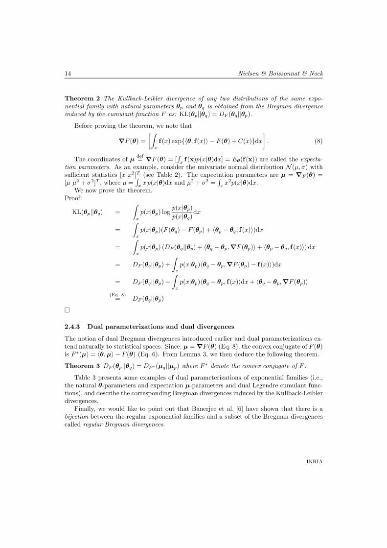
Theorem 2 The Kullback-Leibler divergence of any two distributions of the same expo-nential family with natural parameters θp and θq is obtained from the Bregman divergenceinduced by the cumulant function F as: KL(θp||θq) = DF (θq||θp).

Before proving the theorem, we note that

∇F (θ) =[∫

x

f(x) exp{〈θ, f(x)〉 − F (θ) + C(x)}dx

]. (8)

The coordinates of µdef= ∇F (θ) = [

∫xf(x)p(x|θ)dx] = Eθ(f(x)) are called the expecta-

tion parameters. As an example, consider the univariate normal distribution N (µ, σ) withsufficient statistics [x x2]T (see Table 2). The expectation parameters are µ = ∇F (θ) =[µ µ2 + σ2]T , where µ =

∫x

x p(x|θ)dx and µ2 + σ2 =∫

xx2p(x|θ)dx.

We now prove the theorem.Proof:

KL(θp||θq) =∫

x

p(x|θp) logp(x|θp)p(x|θq)

dx

=∫

x

p(x|θp)(F (θq)− F (θp) + 〈θp − θq, f(x)〉)dx

=∫

x

p(x|θp) (DF (θq||θp) + 〈θq − θp,∇F (θp)〉+ 〈θp − θq, f(x)〉) dx

= DF (θq||θp) +∫

x

p(x|θp)〈θq − θp,∇F (θp)− f(x)〉)dx

= DF (θq||θp)−∫

x

p(x|θp)〈θq − θp, f(x)〉dx + 〈θq − θp,∇F (θp)〉

(Eq. 8)= DF (θq||θp)

�

2.4.3 Dual parameterizations and dual divergences

The notion of dual Bregman divergences introduced earlier and dual parameterizations ex-tend naturally to statistical spaces. Since, µ = ∇F (θ) (Eq. 8), the convex conjugate of F (θ)is F ∗(µ) = 〈θ,µ〉 − F (θ) (Eq. 6). From Lemma 3, we then deduce the following theorem.

Theorem 3 DF (θp||θq) = DF∗(µq||µp) where F ∗ denote the convex conjugate of F .

Table 3 presents some examples of dual parameterizations of exponential families (i.e.,the natural θ-parameters and expectation µ-parameters and dual Legendre cumulant func-tions), and describe the corresponding Bregman divergences induced by the Kullback-Leiblerdivergences.

Finally, we would like to point out that Banerjee et al. [6] have shown that there is abijection between the regular exponential families and a subset of the Bregman divergencescalled regular Bregman divergences.

INRIA


Bernouilli dual divergences: Logistic loss/binary relative entropy

F (θ) = log(1 + exp θ) DF (θ||θ′) = log 1+exp θ1+exp θ′ − (θ − θ′) exp θ′

1+exp θ′ f(θ) = exp θ1+exp θ

= µ

F ∗(µ) = µ log µ + (1 − µ) log(1 − µ) DF∗ (µ′||µ) = µ′ log µ′

µ+ (1 − µ) log 1−µ′

1−µf∗(µ) = log µ

1−µ= θ

Poisson dual divergences: Exponential loss/Unnormalized Shannon entropy

F (θ) = exp θ DF (θ||θ′) = exp θ − exp θ′ − (θ − θ′) exp θ′ f(θ) = exp θ = µ

F ∗(µ) = µ log µ − µ DF∗ (µ′||µ) = µ′ log µ′

µ+ µ − µ′ f∗(µ) = log µ = θ

Table 3: Examples of dual parameterizations of exponential families and their correspondingKullback-Leibler (Bregman) divergences for the Bernoulli and Poisson distributions.

3 Elements of Bregman geometry

In this section, we discuss several basic geometric properties that will be useful when studyingBregman Voronoi diagrams. Specifically, we characterize Bregman bisectors, Bregman ballsand Bregman geodesics. Since Bregman divergences are not symmetric, we describe severaltypes of Bregman bisectors in §3.1. We subsequently characterize Bregman balls by usinga lifting transform that extends a construction well-known in the Euclidean case (§3.2).Finally, we characterize geodesics and show an orthogonality property between bisectorsand geodesics in §3.3.

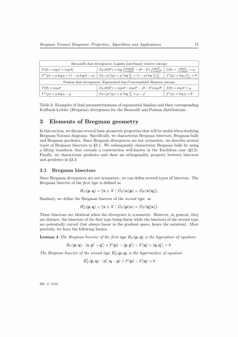
3.1 Bregman bisectors

Since Bregman divergences are not symmetric, we can define several types of bisectors. TheBregman bisector of the first type is defined as

HF (p,q) = {x ∈ X | DF (x||p) = DF (x||q)}.

Similarly, we define the Bregman bisector of the second type as

H ′F (p,q) = {x ∈ X | DF (p||x) = DF (q||x)}.

These bisectors are identical when the divergence is symmetric. However, in general, theyare distinct, the bisectors of the first type being linear while the bisectors of the second typeare potentially curved (but always linear in the gradient space, hence the notation). Moreprecisely, we have the following lemma

Lemma 4 The Bregman bisector of the first type HF (p,q) is the hyperplane of equation:

HF (p,q) : 〈x,p′ − q′〉+ F (p)− 〈p,p′〉 − F (q) + 〈q,q′〉 = 0

The Bregman bisector of the second type H ′F (p,q) is the hypersurface of equation

H ′F (p,q) : 〈x′,q− p〉+ F (p)− F (q) = 0

RR n° 6154


(a hyperplane in the gradient space X ′).

It should be noted that p and q lie necessarily on different sides of HF (p,q) sinceHF (p,q)(p) = −DF (p||q) < 0 and HF (p,q)(q) = DF (q||p) > 0.

From Lemma 3, we know that DF (x||y) = DF∗(y′||x′) where F ∗ is the convex conjugateof F . We therefore have

HF (p,q) = ∇−1F (H ′F∗(q

′,p′)),H ′

F (p,q) = ∇−1F (HF∗(q′,p′)).

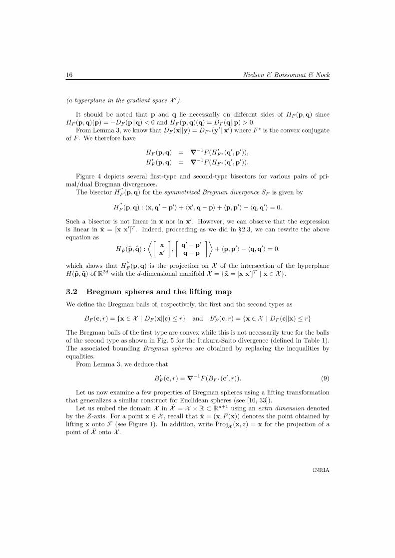
Figure 4 depicts several first-type and second-type bisectors for various pairs of pri-mal/dual Bregman divergences.

The bisector H′′

F (p,q) for the symmetrized Bregman divergence SF is given by

H′′

F (p,q) : 〈x,q′ − p′〉+ 〈x′,q− p〉+ 〈p,p′〉 − 〈q,q′〉 = 0.

Such a bisector is not linear in x nor in x′. However, we can observe that the expressionis linear in x = [x x′]T . Indeed, proceeding as we did in §2.3, we can rewrite the aboveequation as

HF (p, q) :⟨[

xx′

],

[q′ − p′

q− p

]⟩+ 〈p,p′〉 − 〈q,q′〉 = 0.

which shows that H′′

F (p,q) is the projection on X of the intersection of the hyperplaneH(p, q) of R2d with the d-dimensional manifold X = {x = [x x′]T | x ∈ X}.

3.2 Bregman spheres and the lifting map

We define the Bregman balls of, respectively, the first and the second types as

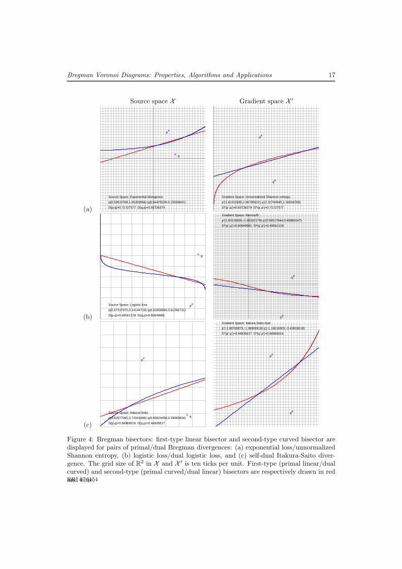
BF (c, r) = {x ∈ X | DF (x||c) ≤ r} and B′F (c, r) = {x ∈ X | DF (c||x) ≤ r}

The Bregman balls of the first type are convex while this is not necessarily true for the ballsof the second type as shown in Fig. 5 for the Itakura-Saito divergence (defined in Table 1).The associated bounding Bregman spheres are obtained by replacing the inequalities byequalities.

From Lemma 3, we deduce that

B′F (c, r) = ∇−1F (BF∗(c′, r)). (9)

Let us now examine a few properties of Bregman spheres using a lifting transformationthat generalizes a similar construct for Euclidean spheres (see [10, 33]).

Let us embed the domain X in X = X × R ⊂ Rd+1 using an extra dimension denotedby the Z-axis. For a point x ∈ X , recall that x = (x, F (x)) denotes the point obtained bylifting x onto F (see Figure 1). In addition, write ProjX (x, z) = x for the projection of apoint of X onto X .

INRIA


Source space X Gradient space X ′

(a)

p

q

Source Space: Exponential divergence

p(0.59510788,1.05359966) q(0.84475539,0.15558641)

D(p,q)=0.71727577 D(q,p)=0.93736374

p’

q’

Gradient Space: Unnormalized Shannon entropy

p’(1.81322655,2.86795622) q’(2.32740845,1.16834289)

D*(p’,q’)=0.93736374 D*(q’,p’)=0.71727577

(b)

p

q

Source Space: Logistic loss

p(0.87337870,0.14144719) q(0.92858669,0.61296731)

D(p,q)=0.49561129 D(q,p)=0.60649981 p’

q’

Gradient Space: Bernouilli

p’(1.93116855,-1.80332178) q’(2.56517944,0.45980247)

D*(p’,q’)=0.60649981 D*(q’,p’)=0.49561129

(c)

p

qSource Space: Itakura-Saito

p(0.52977081,0.72041688) q(0.85824458,0.29083834)

D(p,q)=0.66969016 D(q,p)=0.44835617

p’

q’

Gradient Space: Itakura-Saito dual

p’(-1.88760873,-1.38808518) q’(-1.16516903,-3.43833618)

D*(p’,q’)=0.44835617 D*(q’,p’)=0.66969016

Figure 4: Bregman bisectors: first-type linear bisector and second-type curved bisector aredisplayed for pairs of primal/dual Bregman divergences: (a) exponential loss/unnormalizedShannon entropy, (b) logistic loss/dual logistic loss, and (c) self-dual Itakura-Saito diver-gence. The grid size of R2 in X and X ′ is ten ticks per unit. First-type (primal linear/dualcurved) and second-type (primal curved/dual linear) bisectors are respectively drawn in redand blue.RR n° 6154


(a) (b) (c)

Figure 5: Bregman balls for the Itakura-Saito divergence. The (convex) ball (a) of the firsttype BF (c, r), (b) the ball of the second type B′

F (c, r) with the same center and radius, (c)superposition of the two corresponding bounding spheres.

Let p ∈ X and Hp be the hyperplane tangent to F at point p of equation

z = Hp(x) = 〈x− p,p′〉+ F (p),

and let H↑p denote the halfspace above Hp consisting of the points x = [x z]T ∈ X such that

z > Hp(x). Let σ(c, r) denote either the first-type or second-type Bregman sphere centeredat c with radius r (i.e., ∂BF (c, r) or ∂B′

F (c, r)).The lifted image σ of a Bregman sphere σ is σ = {(x, F (x)),x ∈ σ}. We associate to a

Bregman sphere σ = σ(c, r) of X the hyperplane

Hσ : z = 〈x− c, c′〉+ F (c) + r, (10)

parallel to Hc and at vertical distance r from Hc (see Figure 6). Observe that Hσ coincideswith Hc when r = 0, i.e. when sphere σ is reduced to a single point.

Lemma 5 σ is the intersection of F with Hσ. Conversely, the intersection of any hyper-plane H with F projects onto X as a Bregman sphere. More precisely, if the equation of His z = 〈x,a〉+ b, the sphere is centered at c = ∇−1F (a) and its radius is 〈a, c〉 − F (c) + b.

Proof: The first part of the lemma is a direct consequence of the fact that DF (x||y) ismeasured by the vertical distance from x to Hy (see Lemma 1). For the second part, weconsider the hyperplane H‖ parallel to H and tangent to F . From Eq. 10, we deducea = c′. The equation of H‖ is thus z = 〈x−∇−1F (a),a〉 + F (∇−1F (a)). It follows thatthe divergence from any point of σ to c, which is equal to the vertical distance between Hand H‖, is 〈∇−1F (a),a〉 − F (∇−1F (a)) + b = 〈a, c〉 − F (c) + b. �

INRIA


(a) Squared Euclidean distance (b) Itakura-Saito divergence

Figure 6: Two Bregman circles σ and the associated curves σ obtained by lifting σ ontoF . The curves σ are obtained as the intersection of the hyperplane Hσ with the convexhypersurface F . 3D illustration with (a) the squared Euclidean distance, and (b) the Itakura-Saito divergence.

RR n° 6154


Bregman spheres have been defined as manifolds of codimension 1 of Rd, i.e. hyper-spheres. More generally, we can define the Bregman spheres of codimension k + 1 of Rd

as the Bregman (hyper)spheres of some affine space Z ⊂ Rd of codimension k. The nextlemma shows that Bregman spheres are stable under intersection.

Lemma 6 The intersection of k Bregman spheres σ1, . . . , σk is a Bregman sphere σ. If theσi pairwise intersect transversally, σ = ∩k

i=1σi is a k-Bregman sphere.

Proof: Consider first the case of Bregman spheres of the first type. The k hyperplanesHσi , i = 1, . . . , k intersect along an affine space H of codimension k of Rd+1 that verticallyprojects onto G. Let Gl = G×R be the vertical flat of codimension k that contains G (andH) and write FG = F ∩Gl and HG = H ∩Gl. Note that FG is the graph of the restrictionof F to G and that HG is a hyperplane of Gl. We can therefore apply Lemma 5 in Gl,which proves the lemma for Bregman spheres of the first type.

The case of Bregman spheres of the second type follows from the duality of Eq. 9. �

Union and intersection of Bregman balls

Theorem 4 The union of n Bregman balls has combinatorial complexity Θ(nbd+12 c) and can

be computed in time Θ(n log n + nbd+12 c).

Proof: To each ball, we can associate its bounding Bregman sphere σi which, by Lemma 5,is the projection by ProjX of the intersection of F with a hyperplane Hσi

. The points ofF that are below Hσi

projects onto points that are inside the Bregman ball bounded by σi.Hence, the union of the balls is the projection by ProjX of the complement of F ∩H↑ whereH↑ = ∩n

i=1H↑σi

. H↑ is a convex polytope defined as the intersection of n half-spaces. Thetheorem follows from McMullen’s theorem that bounds the number of faces of a polytope [31],and Chazelle’s optimal convex hull/half-space intersection algorithm [14]. The result for theballs of the second type is deduced from the result for the balls of the first type and theduality of Eq. 9. �

Very similar arguments prove the following theorem (just replace H↑σi

by the comple-mentary halfspace H↓

σi).

Theorem 5 The intersection of n Bregman balls has combinatorial complexity Θ(nbd+12 c)

and can be computed in time Θ(n log n + nbd+12 c).

Circumscribing Bregman spheres. There exists, in general, a unique Bregman spherepassing through d + 1 points of Rd. This is easily shown using the lifting map since, ingeneral, there exists a unique hyperplanes of Rd+1 passing through d + 1 points. The claimthen follows from Lemma 5.

Deciding whether a point x falls inside, on or outside a Bregman sphere σ ∈ Rd passingthrough d + 1 points of p0, ...,pd will be crucial for computing Bregman Voronoi diagramsand associated triangulations. The lifting map immediately implies that such a decision task

INRIA


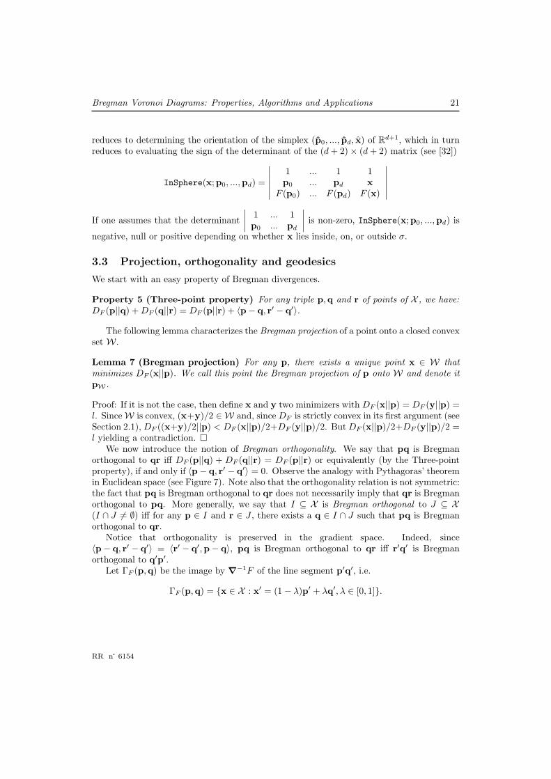
reduces to determining the orientation of the simplex (p0, ..., pd, x) of Rd+1, which in turnreduces to evaluating the sign of the determinant of the (d + 2)× (d + 2) matrix (see [32])

InSphere(x;p0, ...,pd) =

∣∣∣∣∣∣1 ... 1 1p0 ... pd x

F (p0) ... F (pd) F (x)

∣∣∣∣∣∣If one assumes that the determinant

∣∣∣∣ 1 ... 1p0 ... pd

∣∣∣∣ is non-zero, InSphere(x;p0, ...,pd) is

negative, null or positive depending on whether x lies inside, on, or outside σ.

3.3 Projection, orthogonality and geodesics

We start with an easy property of Bregman divergences.

Property 5 (Three-point property) For any triple p,q and r of points of X , we have:DF (p||q) + DF (q||r) = DF (p||r) + 〈p− q, r′ − q′〉.

The following lemma characterizes the Bregman projection of a point onto a closed convexset W.

Lemma 7 (Bregman projection) For any p, there exists a unique point x ∈ W thatminimizes DF (x||p). We call this point the Bregman projection of p onto W and denote itpW .

Proof: If it is not the case, then define x and y two minimizers with DF (x||p) = DF (y||p) =l. SinceW is convex, (x+y)/2 ∈ W and, since DF is strictly convex in its first argument (seeSection 2.1), DF ((x+y)/2||p) < DF (x||p)/2+DF (y||p)/2. But DF (x||p)/2+DF (y||p)/2 =l yielding a contradiction. �

We now introduce the notion of Bregman orthogonality. We say that pq is Bregmanorthogonal to qr iff DF (p||q) + DF (q||r) = DF (p||r) or equivalently (by the Three-pointproperty), if and only if 〈p− q, r′ − q′〉 = 0. Observe the analogy with Pythagoras’ theoremin Euclidean space (see Figure 7). Note also that the orthogonality relation is not symmetric:the fact that pq is Bregman orthogonal to qr does not necessarily imply that qr is Bregmanorthogonal to pq. More generally, we say that I ⊆ X is Bregman orthogonal to J ⊆ X(I ∩ J 6= ∅) iff for any p ∈ I and r ∈ J , there exists a q ∈ I ∩ J such that pq is Bregmanorthogonal to qr.

Notice that orthogonality is preserved in the gradient space. Indeed, since〈p− q, r′ − q′〉 = 〈r′ − q′,p− q〉, pq is Bregman orthogonal to qr iff r′q′ is Bregmanorthogonal to q′p′.

Let ΓF (p,q) be the image by ∇−1F of the line segment p′q′, i.e.

ΓF (p,q) = {x ∈ X : x′ = (1− λ)p′ + λq′, λ ∈ [0, 1]}.

RR n° 6154


W

wpW

p

Figure 7: Generalized Pythagoras’ theorem for Bregman divergences: The projection pWof point p to a convex subset W ⊆ X . For convex subset W, we have DF (w||p) ≥DF (w||pW) + DF (pW ||p) (with equality for and only for affine sets W).

By analogy, we rename the line segment pq as

Λ(p,q) = {x ∈ X : x = (1− λ)p + λq, λ ∈ [0, 1]}

In the Euclidean case (F (x) = 12‖x‖

2), ΓF (p,q) = Λ(p,q) is the unique geodesic pathjoining p to q and it is orthogonal to the bisector HF (p,q). For general Bregman diver-gences, we have similar properties as shown next.

Lemma 8 ΓF (p,q) is Bregman orthogonal to the Bregman bisector HF (p,q) while Λ(p,q)is Bregman orthogonal to HF∗(p,q).

Proof: Since p and q lie on different sides of HF (p,q), ΓF (p,q) must intersect HF (p,q).Fix any distinct x ∈ Γ(p,q) and y ∈ HF (p,q), and let t ∈ Γ(p,q) ∩ HF (p,q). To provethe first part of the lemma, we need to show that 〈y − t,x′ − t′〉 = 0.

Since t and x both belong to ∈ ΓF (p,q), we have t′ − x′ = λ(p′ − q′), for some λ ∈ R,and, since y and t belong to HF (p,q), we deduce from the equation of HF (p,q) that〈y − t,p′ − q′〉 = 0. We conclude that 〈y − t,x′ − t′〉 = 0, which proves that ΓF (p,q) isindeed Bregman orthogonal to HF (p,q).

The second part of the lemma is easily proved by using the fact that orthogonality ispreserved in the gradient space as noted above. �

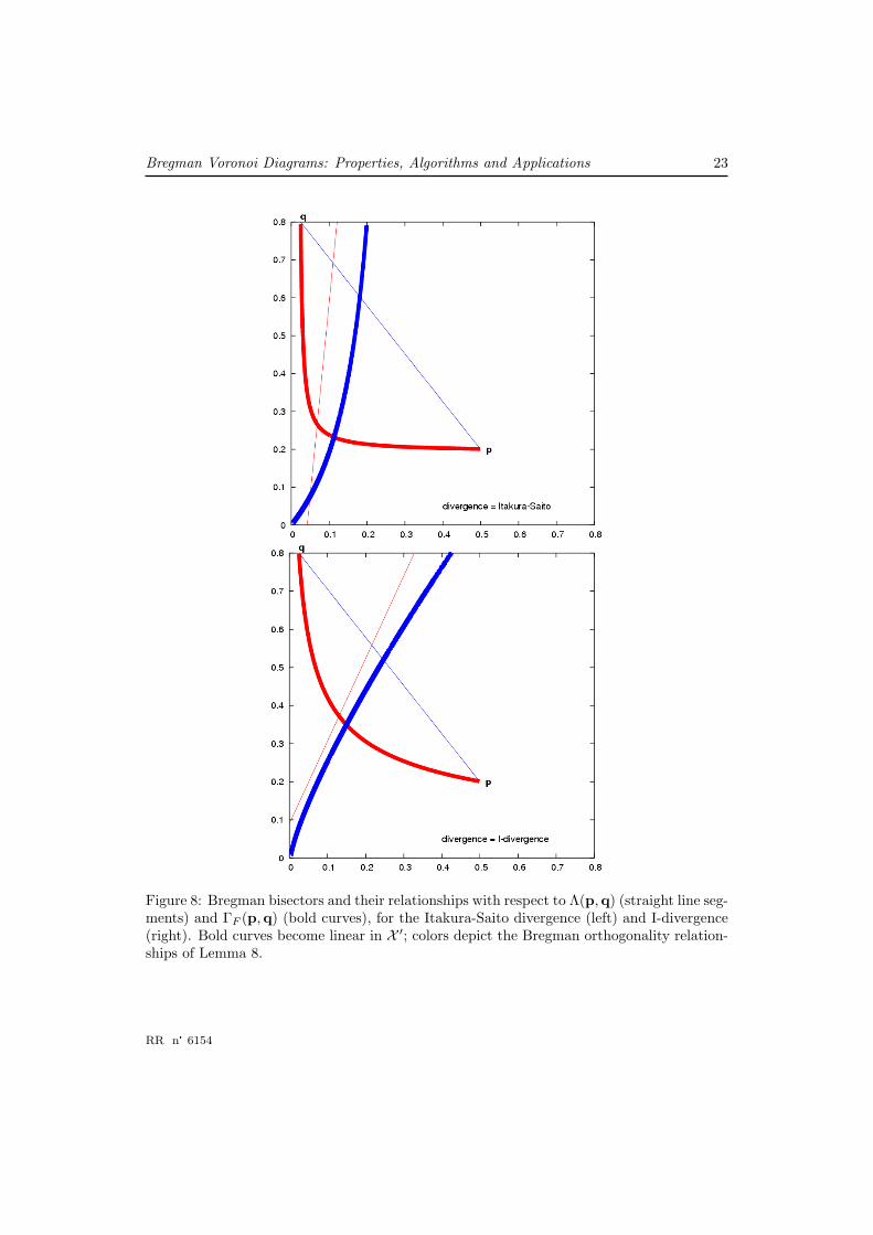
Figure 8 shows Bregman bisectors and their relationships with respect to Λ(p,q) andΓF (p,q).

We now focus on characterizing Bregman geodesics. First, recall that a parameterizedcurve C between two points p0 and p1 is defined as a set C = {pλ}1λ=0, which is continuous.In Riemannian geometry, geodesics are the curves that minimize the arc length with respectto the Riemannian metric [1, 27]. Since embedding X with a Bregman divergence does notyield a metric space, we define the following curve lengths:

`Γ(C) =∫ 1

λ=0

DF (p0||pλ)dλ , (11)

INRIA


Figure 8: Bregman bisectors and their relationships with respect to Λ(p,q) (straight line seg-ments) and ΓF (p,q) (bold curves), for the Itakura-Saito divergence (left) and I-divergence(right). Bold curves become linear in X ′; colors depict the Bregman orthogonality relation-ships of Lemma 8.

RR n° 6154


`Λ(C) =∫ 1

λ=0

DF (pλ||p0)dλ. (12)

We now characterize the dual pair of geodesics and their lengths as follows:

Lemma 9 Curve ΓF (p0,p1) (respectively straight line segment Λ(p0,p1)) minimizes∫ 1

λ=0DF (p0||pλ)dλ (respectively

∫ 1

λ=0DF (pλ||p0)dλ) over all curves C = {pλ}1λ=0.

Proof: For any curve C between p0 and p1, we measure the `Γ length as `Γ(C) =∫λ

DF (pλ||p0)dλ. Fix some inner point p ∈ ΓF (p0,p1)\{p0,p1}. From the three-pointproperty (Property 5), the set of points {y ∈ X | DF (y||p0) = DF (y||p) + DF (p||p0)}is the hyperplane Hp : 〈y,h〉 = b (h is a perpendicular vector to the hyperplane) whichsplits X into two open half-spaces H+

p : 〈y,h〉 > b, and H−p : 〈y,h〉 < b. Now, Hp in-

tersects Γ(p0,p1) since Hp separates p0 from p1. Indeed, Hp(p0) = 〈p0 − p,p′0 − p′〉 =DF (p0||p) + DF (p||p0) > 0 and Hp(p1) = 〈p1 − p,p′0 − p′〉 = λ−1

λ 〈p1 − p,p′1 − p′〉 < 0where p′ = λp′0 + (1− λ)p′1 (with λ ∈]0, 1[). Therefore any connected path C joining p0 top1 has to intersect Hp.

To finish up, consider function f : [0, 1] → C with f(0) = p0, f(1) = p1, and f(λ) ∈C ∩Hpλ

otherwise, where it is understood that pλ is hereafter a point of ΓF (p0,p1). Sincef(λ) ∈ Hp(λ), we have DF (f(λ)||p0) = DF (f(λ)||pλ) + DF (pλ||p0) ≥ DF (pλ||p0), withequality if and only if f(λ) = pλ. Thus we have

`Γ(ΓF (p0,p1)) =∫ 1

λ=0

DF (pλ||p0)dλ ≤∫ 1

λ=0

DF (f(λ)||p0)dλ ≤ `Γ(C) .

The case of Λ(p0,p1) follows similarly from Legendre convex duality.�

Corollary 1 Since ΓF (p0,p1) = ΓF (p1,p0) (respectively, since Λ(p0,p1) = Λ(p1,p0))we deduce that ΓF (p0,p1) minimizes also

∫ 1

λ=0DF (p1||pλ)dλ (respectively, minimizes also∫ 1

λ=0DF (pλ||p1)dλ) over all curves C = {pλ}1λ=0.

Observe also that ΓF (p,q) is the unique geodesic path joining p to q in X for the metricimage by ∇−1F of the Euclidean metric.

Finally, we give a characterization of these geodesics in information-theoretic spaces.Recall that Banerjee et al. [6] showed that Bregman divergences are in bijection with expo-nential families. This was emphasized by Theorem 2 that proved that the Kullback-Leiblerdivergence of probability density functions of the same exponential family EF is a Bregmandivergence DF for the cumulant function F . From this standpoint, Λ(p,q) and ΓF (p,q)minimize the total Kullback-Leibler divergence, a characteristic that we choose to call theinformation length of a curve. Since the Kullback-Leibler divergence is not symmetric, thisjustifies for the existence of two geodesics, one which appears to be linear when parame-terized with the natural affine coordinate system (θ), and the other that is linear in theexpectation affine coordinate system (µ). See also [1].

INRIA


Corollary 2 Suppose p(.|θ0) and p(.|θ1) are probability density functions of the same expo-nential family EF . Then ΓF (θ0,θ1) (resp. Λ(θ0,θ1)) minimizes `Γ(C) =

∫ 1

λ=0KL(θ0||θλ)dλ

(resp. `Λ(C) =∫ 1

λ=0KL(θλ||θ0)dλ) over all curves C = {p(.|θλ)}1λ=0.

4 Bregman Voronoi diagrams

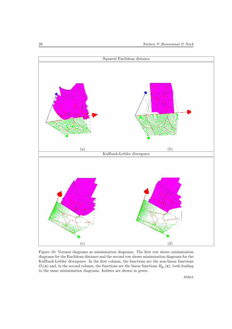
Let S = {p1, ...,pn} be a finite point set of X ⊂ Rd. To each point pi is attached a d-variatecontinuous function Di defined over X . We define the lower envelope of the functions asthe graph of min1≤i≤n Di and their minimization diagram as the subdivision of X into cellssuch that, in each cell, arg mini fi is fixed.

The Euclidean Voronoi diagram is the minimization diagram for Di(x) = ‖x− pi‖2. Inthis section, we introduce Bregman Voronoi diagrams as minimization diagrams of Bregmandivergences (see Figure 10).

We define three types of Bregman Voronoi diagrams in §4.1. We establish a correspon-dence between Bregman Voronoi diagrams and polytopes in §4.2 and with power diagramsin §4.3. These correspondences lead to tight combinatorial bounds and efficient algorithms.Finally, in §4.4, we give two generalizations of Bregman Voronoi diagrams; k-order and k-bagdiagrams.

We note S ′ = {∇F (pi), i = 1, . . . , n} the gradient point set associated to S.

4.1 Three types of diagrams

Because Bregman divergences are not necessarily symmetric, we associate to each site pi

two types of distance functions, namely Di(x) = DF (x||pi) and D′i(x) = DF (pi||x). The

minimization diagram of the Di, i = 1, . . . , n, is called the first-type Bregman Voronoidiagram of S, which we denote by vorF (S). The d-dimensional cells of this diagram are in1-1 correspondence with the sites pi and the d-dimensional cell of pi is defined as

vorF (pi)def= {x ∈ X | DF (x||pi) ≤ DF (x||pj) ∀pj ∈ S.}

Since the Bregman bisectors of the first-type are hyperplanes, the cells of any diagramof the first-type are convex polyhedra. Therefore, first-type Bregman Voronoi diagrams areaffine diagrams [4, 5].

Similarly, the minimization diagram of the D′i, i = 1, . . . , n, is called the second-type

Bregman Voronoi diagram of S, which we denote by vor′F (S). A cell in vor′F (S) is associatedto each site pi and is defined as above with permuted divergence arguments:

vor′F (pi)def= {x ∈ X | DF (pi||x) ≤ DF (pj ||x) ∀pj ∈ S.}

In contrast with the diagrams of the first-type, the diagrams of the second type have, ingeneral, curved faces.

RR n° 6154


(a) (b)

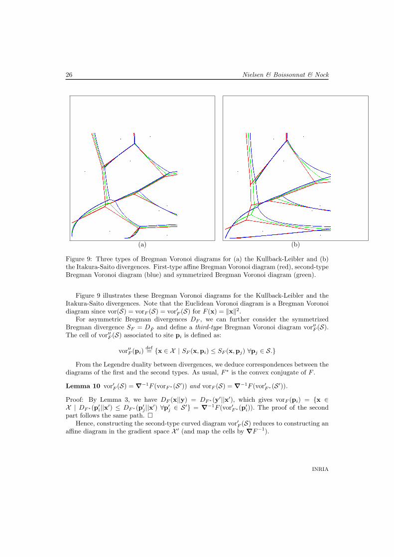
Figure 9: Three types of Bregman Voronoi diagrams for (a) the Kullback-Leibler and (b)the Itakura-Saito divergences. First-type affine Bregman Voronoi diagram (red), second-typeBregman Voronoi diagram (blue) and symmetrized Bregman Voronoi diagram (green).

Figure 9 illustrates these Bregman Voronoi diagrams for the Kullback-Leibler and theItakura-Saito divergences. Note that the Euclidean Voronoi diagram is a Bregman Voronoidiagram since vor(S) = vorF (S) = vor′F (S) for F (x) = ‖x‖2.

For asymmetric Bregman divergences DF , we can further consider the symmetrizedBregman divergence SF = DF and define a third-type Bregman Voronoi diagram vor′′F (S).The cell of vor′′F (S) associated to site pi is defined as:

vor′′F (pi)def= {x ∈ X | SF (x,pi) ≤ SF (x,pj) ∀pj ∈ S.}

From the Legendre duality between divergences, we deduce correspondences between thediagrams of the first and the second types. As usual, F ∗ is the convex conjugate of F .

Lemma 10 vor′F (S) = ∇−1F (vorF∗(S ′)) and vorF (S) = ∇−1F (vor′F∗(S ′)).

Proof: By Lemma 3, we have DF (x||y) = DF∗(y′||x′), which gives vorF (pi) = {x ∈X | DF∗(p′i||x′) ≤ DF∗(p′j ||x′) ∀p′j ∈ S ′} = ∇−1F (vor′F∗(p

′i)). The proof of the second

part follows the same path. �Hence, constructing the second-type curved diagram vor′F (S) reduces to constructing an

affine diagram in the gradient space X ′ (and map the cells by ∇F−1).

INRIA


Let us end this section by considering the case of symmetrized Bregman divergencesintroduced in §2.3: SF (p,q) = DF (p||q) = DF (q||p) where F is a 2d-variate function andx = [x x′]T . As already noted in §2.3, x lies on the d-manifold X = {[x x′]T | x ∈ Rd}. Itfollows that the symmetrized Voronoi diagram vor′′F (S) is the projection of the restrictionto X of the affine diagram vorF (S) of R2d where S = {pi,pi ∈ S}. Hence, computing thesymmetrized Voronoi diagram of S reduces to:

1. computing the first-type Bregman Voronoi diagram vorF (S) of R2d,

2. intersecting the cells of this diagram with the manifold X , and

3. projecting all points of vorF (S) ∩ X to X by simply dropping the last d coordinates.

4.2 Bregman Voronoi diagrams from polytopes

Let Hpi , i = 1, . . . , n, denote the hyperplanes of X defined in §3.2. For any x ∈ X , we havefollowing Lemma 1

DF (x||pi) ≤ DF (x||pj) ⇐⇒ Hpi(x) ≥ Hpj (x).

The first-type Bregman Voronoi diagram of S is therefore the maximization diagram of the nlinear functions Hpi(x) whose graphs are the hyperplanes Hpi (see Figure 10). Equivalently,we have

Theorem 6 The first-type Bregman Voronoi diagram vorF (S) is obtained by projecting byProjX the faces of the (d + 1)-dimensional convex polyhedron H = ∩iH

↑pi

of X+ onto X .

From McMullen’s upperbound theorem [31] and Chazelle’s optimal half-space intersec-tion algorithm [14], we know that the intersection of n halfspaces of Rd has complexityΘ(nb

d2 c) and can be computed in optimal-time Θ(n log n + nb

d2 c) for any fixed dimension d.

From Theorem 6 and Lemma 10, we then deduce the following theorem.

Theorem 7 The Bregman Voronoi diagrams of type 1 or 2 of a set of n d-dimensionalpoints have complexity Θ(nb

d+12 c) and can be computed in optimal time Θ(n log n + nb

d+12 c).

The third-type Bregman Voronoi diagram for the symmetrized Bregman divergence of a setof n d-dimensional points has complexity O(nd) and can be obtained in time O(nd).

Apart from Chazelle’s algorithm, several other algorithms are known for constructing theintersection of a finite number of halfplanes, especially in the 2- and 3-dimensional cases.See [10, 5] for further references.

RR n° 6154


Squared Euclidean distance

(a) (b)Kullback-Leibler divergence

(c) (d)

Figure 10: Voronoi diagrams as minimization diagrams. The first row shows minimizationdiagrams for the Euclidean distance and the second row shows minimization diagrams for theKullback-Leibler divergence. In the first column, the functions are the non-linear functionsDi(x) and, in the second column, the functions are the linear functions Hpi

(x), both leadingto the same minimization diagrams. Isolines are shown in green.

INRIA


4.3 Bregman Voronoi diagrams from power diagrams

The power distance of a point x to a Euclidean ball B = B(p, r) is defined as ||p−x||2− r2.Given n balls Bi = B(pi, ri), i = 1, . . . , n, the power diagram (or Laguerre diagram) ofthe Bi is defined as the minimization diagram of the corresponding n functions Di(x) =||pi − x||2 − r2. The power bisector of any two balls B(pi, ri) and B(pj , rj) is the radicalhyperplane of equation 2〈x,pj − pi〉+||pi||2−||qj ||2+r2

j−r2i = 0. Thus power diagrams are

affine diagrams. In fact, as shown by Aurenhammer [3, 10], any affine diagram is identicalto the power diagram of a set of corresponding balls. In general, some balls may have anempty cell in their power diagram.

Since Bregman Voronoi diagrams of the first type are affine diagrams, Bregman Voronoidiagrams are power diagrams [3, 10] in disguise. The following theorem makes precise thecorrespondence between Bregman Voronoi diagrams and power diagrams (see Figure 11).

Theorem 8 The first-type Bregman Voronoi diagram of n sites is identical to the powerdiagram of the n Euclidean spheres of equations

〈x− p′i,x− p′i〉 = 〈p′i,p′i〉+ 2(F (pi)− 〈pi,p′i〉), i = 1, . . . , n.

Proof: We have

DF (x||pi) ≤ DF (x||pj)⇐⇒ −F (pi)− 〈x− pi,p′i〉 ≤ −F (pj)− 〈x− pj ,p′j〉

Multiplying twice the last inequality, and adding 〈x,x〉 to both sides yields

〈x,x〉 − 2〈x,p′i〉 − 2F (pi) + 2〈pi,p′i〉 ≤ 〈x,x〉 − 2〈x,p′j〉 − 2F (pj) + 2〈pj ,p′j〉⇐⇒ 〈x− p′i,x− p′i〉 − r2

i ≤ 〈x− p′j ,x− p′j〉 − r2j ,

where r2i = 〈p′i,p′i〉+ 2(F (pi)− 〈pi,p′i〉) and r2

j = 〈p′j ,p′j〉+ 2(F (pj)− 〈pj ,p′j〉). The lastinequality means that the power of x with respect to the Euclidean (possibly imaginary) ballB(p′i, ri) is no more than the power of x with respect to the Euclidean (possibly imaginary)ball B(p′j , rj). �

As already noted, for F (x) = 12‖x‖

2, vorF (S) is the Euclidean Voronoi diagram of S.Accordingly, the theorem says that the centers of the spheres are the pi and r2

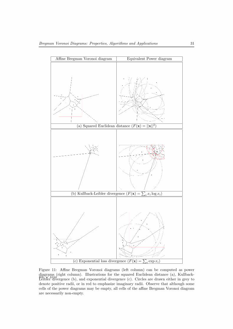
i = 0 sincep′i = pi. Figure 11 displays affine Bregman Voronoi diagrams3 and their equivalent powerdiagrams for the squared Euclidean, Kullback-Leibler and exponential divergences.

Note that although the affine Bregman Voronoi diagram obtained by scaling the diver-gence DF by a factor λ > 0 does not change, the equivalent power diagrams are not strictussenso identical since the centers of corresponding Euclidean balls and radii are mapped

3See Java� applet at http://www.csl.sony.co.jp/person/nielsen/BVDapplet/

RR n° 6154

http://www.csl.sony.co.jp/person/nielsen/BVDapplet/


differently. See the example of the squared Euclidean distance depicted in Figure 11(a).Since Power diagrams are well defined “everywhere”, this equivalence relationship providesa natural way to extend the scope of definition of Bregman Voronoi diagrams from X ⊂ Rd

to the full space Rd. (That is, Bregman Voronoi diagrams are power diagrams restricted toX .)

To check that associated balls may be potentially imaginary, consider for example, theKullback-Leibler divergence. The Bregman generator function is F (x) =

∑i xi log xi and

the gradient is ∇F (x) = [log x1 ... log xd]T . A point p = [p1 ... pd]T ∈ X maps to aEuclidean ball of center p′ = [log p1 ... log pd]T with radius r2

p =∑

i(log2 pi−2pi). Thus forpoints p with coordinates pi > 1

2 log p2i for i ∈ {1, ..., d}, the squared radius r2

p is negative,yielding an imaginary ball. See Figure 11(b).

It is also to be observed that not all power diagrams are Bregman Voronoi diagrams.Indeed, in power diagrams, some balls may have empty cells while each site has necessarilya non empty cell in a Bregman Voronoi diagram (See Figure 11 and Section 4.4 for a furtherdiscussion at this point).

Since there exist fast algorithms for constructing power diagrams [36], Theorem 8 pro-vides an efficient way to construct Bregman Voronoi diagrams.

4.4 Generalized Bregman divergences and their Voronoi diagrams

Weighted Bregman Voronoi diagrams

Let us associate to each site pi a weight wi ∈ R. We define the weighted divergence betweentwo weighted points as WDF (pi||pj)

def= DF (pi||pj) + wi − wj . We can define bisectorsand weighted Bregman Voronoi diagrams in very much the same way as for non weighteddivergences. The Bregman Voronoi region associated to the weighted point (pi, wi) is definedas

vorF (pi, wi) = {x ∈ X | DF (x||pi) + wi ≤ DF (x||pj) + wj ∀pj ∈ S}.

Observe that the bisectors of the first-type diagrams are still hyperplanes and that thediagram can be obtained as the projection of a convex polyhedron or as the power diagramof a finite set of balls. The only difference with respect to the construction of Section 4.2is the fact that now the hyperplanes Hpi are no longer tangent to F since they are shiftedby a z-displacement of length wi. Hence Theorem 7 extends to weighted Bregman Voronoidiagrams.

Theorem 9 The weighted Bregman Voronoi diagrams of type 1 or 2 of a set of n

d-dimensional points have complexity Θ(nbd+12 c) and can be computed in optimal time

Θ(n log n + nbd+12 c).

k-order Bregman Voronoi diagrams

We define the k-order Bregman Voronoi diagram of n punctual sites of X as the subdivisionof X into cells such that each cell is associated to a subset T ⊂ S of k sites and consists of

INRIA


Affine Bregman Voronoi diagram Equivalent Power diagram

(a) Squared Euclidean distance (F (x) = ||x||2)

(b) Kullback-Leibler divergence (F (x) =∑

i xi log xi)

(c) Exponential loss divergence (F (x) =∑

i expxi)

Figure 11: Affine Bregman Voronoi diagrams (left column) can be computed as powerdiagrams (right column). Illustrations for the squared Euclidean distance (a), Kullback-Leibler divergence (b), and exponential divergence (c). Circles are drawn either in grey todenote positive radii, or in red to emphasize imaginary radii. Observe that although somecells of the power diagrams may be empty, all cells of the affine Bregman Voronoi diagramare necessarily non-empty.

RR n° 6154


the points of X whose divergence to any site in T is less than the divergence to the sites notin T . Similarly to the case of higher-order Euclidean Voronoi diagrams, we have:

Theorem 10 The k-order Bregman Voronoi diagram of n d-dimensional points is aweighted Bregman Voronoi diagram.

Proof: Let S1,S2, . . . denote the subsets of k points of S and write

Di(x) =1k

∑pj∈Si

DF (x||pj)

= F (x)− 1k

∑pj∈Si

F (pj) +1k

∑pj∈Si

〈x− pj ,p′j〉

= F (x)− F (ci)− 〈x− ci, c′i〉+ wi

= WDF (x||ci)

where ci = ∇−1F(

1k

∑j∈Si

p′j)

and the weight associated to ci is wi = F (ci)− 〈ci, c′i〉 −1k

∑j∈Si

(F (pj) + 〈pj ,p′j〉

).

Hence, Si is the set of the k nearest neighbors of x iff Di(x) ≤ Dj(x) for all j or,equivalently, iff x belongs to the cell of ci in the weighted Bregman Voronoi diagram of theci. �

k-bag Bregman Voronoi diagrams

Let F1, ..., Fk be k strictly convex and differentiable functions, and α = [α1 ... αk]T ∈ Rk+

a vector of positive weights. Consider the d-variate function Fα =∑k

l=1 αlFl. By virtueof the positive additivity property rule of Bregman basis functions (Property 3), DFα

is aBregman divergence.

Now consider a set S = {p1, ...,pn} of n points of Rd. To each site pi, we associate aweight vector αi = [α(1)

i ... α(k)i ]T inducing a Bregman divergence DFαi

(x||pi)def= Dαi

(x||pi)anchored at that site. Let us consider the first-type of k-bag Bregman Voronoi diagram (k-bag BVD for short). The first-type bisector KF (pi,pj) of two weighted points (pi,αi) and(pj ,αj) is the locus of points x at equidivergence to pi and pj . That is, KF (pi,pj) = {x ∈X | Dαi

(x||pi) = Dαj(x||pj)}. The equation of the bisector is simply obtained using the

definition of Bregman divergences (Eq. 1) as

Fαi(x)− Fαi(pi)− 〈x− pi,∇Fαi(pi)〉 = Fαj (x)− Fαj (pj)− 〈x− pj ,∇Fαi(pj)〉.

This yields the equation of the first-type bisector KF (pi,pj)

k∑l=1

(α(l)i −α

(l)j )Fl(x)− 〈x,∇Fαj (pj)−∇Fαi(pi)〉+ c = 0, (13)

INRIA


where c is a constant depending on weighted sites (pi,αi) and (pj ,αj). Note that theequation of the first-type k-bag BVD bisector is linear if and only if αi = αj (i.e., the caseof standard BVDs).

Let us consider the linearization lifting x 7→ x = [x F1(x) ... Fk(x)]T that maps a pointx ∈ Rd into a point x in Rd+k. Then Eq. 13 becomes linear, namely 〈x,a〉+ c = 0 with

a =[

∇Fαj(pj)−∇Fαi

(pi)αi −αj

]∈ Rd+k.

That is, first-type bisectors of a k-bag BVD are hyperplanes of Rd+k. Therefore thecomplexity of a k-bag Voronoi diagram is at most O(nb

k+d2 c), since it can be obtained

as the intersection of the affine Voronoi diagram in Rd+k with the convex d-dimensionalsubmanifold {x = [x F1(x) ... Fk(x)]T | x ∈ Rd}.

Theorem 11 The k-bag Voronoi diagram (for k > 1) on a bag of d-variate Bregman di-vergences of a set of n points of Rd has combinatorial complexity O(nb

k+d2 c) and can be

computed within the same time bound.

Further, using the Legendre transform, we define a second-type (dual) k-bag BVD. Wehave ∇Fα =

∑kl=1 αl∇Fl and F ∗

α =∫

∇F−1α . (Observe that F ∗

α 6=∑k

l=1 αlF∗l in general.)

k-bag Bregman Voronoi diagrams are closely related to the anisotropic diagrams ofLabelle and Shewchuk [27] that associate to each point x ∈ X a metric tensor Mx

which tells how lengths and angles should be measured from the local perspective ofx. Labelle and Shewchuk relies on a deformation tensor (ideally defined everywhere)to compute the distance between any two points p and q from the perspective of x asdx(p,q) =

√(p− q)T Mx(p− q). Let dx(p) = dx(x,p). The anisotropic Voronoi diagram,

which approximates the ideal but computationally prohibitive Riemannian Voronoi diagram,is defined as the arrangement of the following anisotropic Voronoi cells:

Vor(pi) = {x ∈ X | dpi(x) ≤ dpj

(x) ∀j ∈ {1, ..., n}}, ∀i ∈ {1, ..., n}.

It follows that all anisotropic Voronoi cells are non-empty as it is the case for k-bagBregman Voronoi diagrams.

Hence, the site weights of a k-bag Bregman Voronoi diagram sparsely define a tensordivergence that indicates how divergences should be measured locally from the respective bagof divergences. Noteworthy, our study of k-bag Bregman Voronoi diagrams shows that theanisotropic Voronoi diagram also admits a second-type anisotropic Voronoi diagram, inducedby the respective dual Legendre functions of the Bregman basis functions of the quadraticdistance monomials. The Legendre dual of a quadratic distance function dM(p,q) = (p −q)T M(p−q) induced by positive-definite matrix M is the quadratic distance dM−1 . (MatrixM is itself usually obtained as the inverse of a variance-covariance matrix Σ in so-calledMahalanobis distances.)

RR n° 6154


Figure 12: Ordinary Voronoi diagram (red) and geometric dual Delaunay triangulation(blue).

5 Bregman triangulations

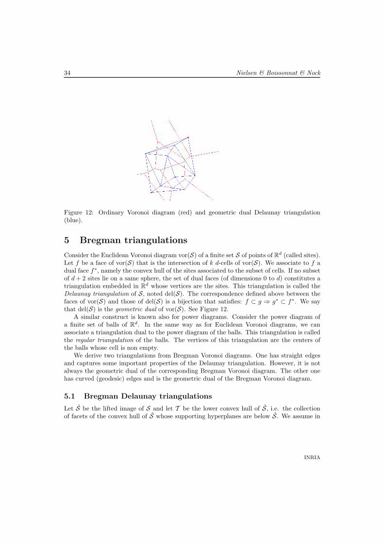
Consider the Euclidean Voronoi diagram vor(S) of a finite set S of points of Rd (called sites).Let f be a face of vor(S) that is the intersection of k d-cells of vor(S). We associate to f adual face f∗, namely the convex hull of the sites associated to the subset of cells. If no subsetof d + 2 sites lie on a same sphere, the set of dual faces (of dimensions 0 to d) constitutes atriangulation embedded in Rd whose vertices are the sites. This triangulation is called theDelaunay triangulation of S, noted del(S). The correspondence defined above between thefaces of vor(S) and those of del(S) is a bijection that satisfies: f ⊂ g ⇒ g∗ ⊂ f∗. We saythat del(S) is the geometric dual of vor(S). See Figure 12.

A similar construct is known also for power diagrams. Consider the power diagram ofa finite set of balls of Rd. In the same way as for Euclidean Voronoi diagrams, we canassociate a triangulation dual to the power diagram of the balls. This triangulation is calledthe regular triangulation of the balls. The vertices of this triangulation are the centers ofthe balls whose cell is non empty.

We derive two triangulations from Bregman Voronoi diagrams. One has straight edgesand captures some important properties of the Delaunay triangulation. However, it is notalways the geometric dual of the corresponding Bregman Voronoi diagram. The other onehas curved (geodesic) edges and is the geometric dual of the Bregman Voronoi diagram.

5.1 Bregman Delaunay triangulations

Let S be the lifted image of S and let T be the lower convex hull of S, i.e. the collectionof facets of the convex hull of S whose supporting hyperplanes are below S. We assume in

INRIA


Figure 13: Bregman Delaunay triangulation as the projection of the convex polyhedron T .

this section that S is in general position if there is no subset of d + 2 points lying on a sameBregman sphere. Equivalently (see Lemma 5), S is in general position if no subset of d + 2points pi lying on a same hyperplane.

Under the general position assumption, each vertex of H = ∩iH↑pi

is the intersectionof exactly d + 1 hyperplanes and the faces of T are all simplices. Moreover the verticalprojection of T is a triangulation delF (S) = ProjX (T ) of S embedded in X ⊆ Rd. Indeed,since the restriction of ProjX to T is bijective, delF (S) is a simplicial complex embeddedin X . Moreover, since F is convex, delF (S) covers the (Euclidean) convex hull of S, andthe set of vertices of T consists of all the pi. Consequently, the set of vertices of delF (S)is S. We call delF (S) the Bregman Delaunay triangulation of S (see Fig. 13). WhenF (x) = ||x||2, delF (S) is the Delaunay triangulation dual to the Euclidean Voronoi diagram.This duality property holds for symmetric Bregman divergences (via polarity) but not forgeneral Bregman divergences.

We say that a Bregman sphere σ is empty if the open ball bounded by σ does not containany point of S. The following theorem extends a similar well-known property for Delaunaytriangulations whose proof (see, for example [10]) can be extended in a straightforward wayto Bregman triangulations using the lifting map introduced in Section 3.2.

Theorem 12 The first-type Bregman sphere circumscribing any simplex of delF (S) isempty. delF (S) is the only triangulation of S with this property when S is in general position.

Several other properties of Delaunay triangulations extend to Bregman triangulations.We list some of them.

RR n° 6154


Theorem 13 (Empty ball) Let ν be a subset of at most d + 1 indices in {1, . . . , n}. Theconvex hull of the associated points pi, i ∈ ν, is a simplex of the Bregman triangulation ofS iff there exists an empty Bregman sphere σ passing through the pi, i ∈ ν.

The next property exhibits a local characterization of Bregman triangulations. Let T (S)be a triangulation of S. We say that a pair of adjacent facets f1 = (f,p1) and f2 = (f,p2)of T (S) is regular iff p1 does not belong to the open Bregman ball circumscribing f2 andp2 does not belong to the open Bregman ball circumscribing f1 (the two statements areequivalent for symmetric Bregman divergences).

Theorem 14 (Locality) Any triangulation of a given set of points S (in general position)whose pairs of facets are all regular is the Bregman triangulation of S.

Let S be a given set of points, delF (S) its Bregman triangulation, and T (S) the set ofall triangulations of S. We define the Bregman radius of a d-simplex τ as the radius notedr(τ) of the smallest Bregman ball containing τ . The following result is an extension of aresult due to Rajan for Delaunay triangulations [37].

Theorem 15 (Optimality) We have delF (S) = minT∈T (S) maxτ∈T r(τ).

The proof mimics Rajan’s proof [37] for the case of Delaunay triangulations.

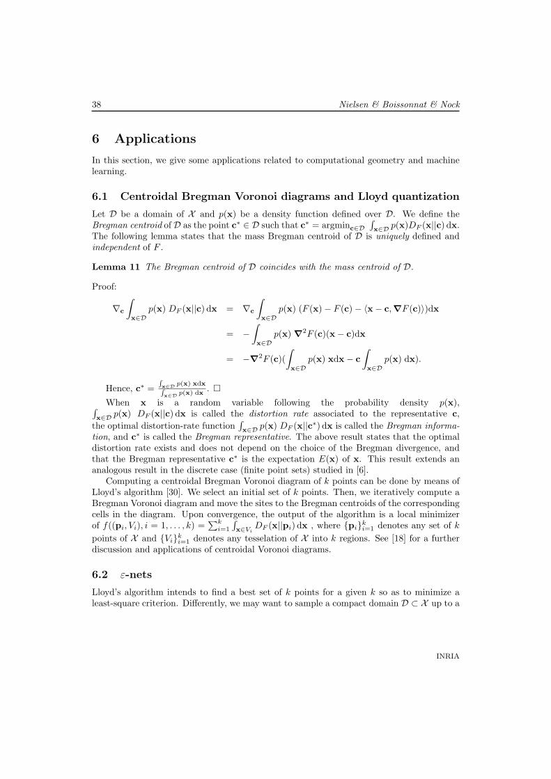
5.2 Bregman geodesic triangulations

We have seen in Section 4.3 that the Bregman Voronoi of a set of points S is the powerdiagram of a set of balls B′ centered at the points of S ′ (Theorem 8). Write regF (B′) for thedual regular triangulation dual to this power diagram. This triangulation4 is embedded inX ′ and has the points of S ′ as its vertices (see Figure 14). The image of this triangulation by∇−1F is a curved triangulation whose vertices are the points of S. The edges of this curvedtriangulation are geodesic arcs joining two sites (see Section 3.3). We call it the Bregmangeodesic triangulation of S, noted del′F (S) (see Figure 15).

Theorem 16 The Bregman geodesic triangulation del′F (S) is the geometric dual of the 1st-type Bregman Voronoi diagram of S.

Proof: We have, noting∗≡ for the dual mapping, and using Theorem 8

vorF (S) ≡ pow(B′) ∗≡ reg(B′) = ∇F (del′F (S)).

�Observe that del′F (S) is, in general, distinct from delF (S), the Bregman Delaunay tri-

angulation introduced in the previous section. However, when the divergence is symmetric,both triangulations are combinatorially equivalent and dual to the Bregman Voronoi diagramof S. Moreover, they coincide exactly when F is the squared Euclidean distance.

4Applet at http://www.csl.sony.co.jp/person/nielsen/BVDapplet/

INRIA

http://www.csl.sony.co.jp/person/nielsen/BVDapplet/


(a) (b)

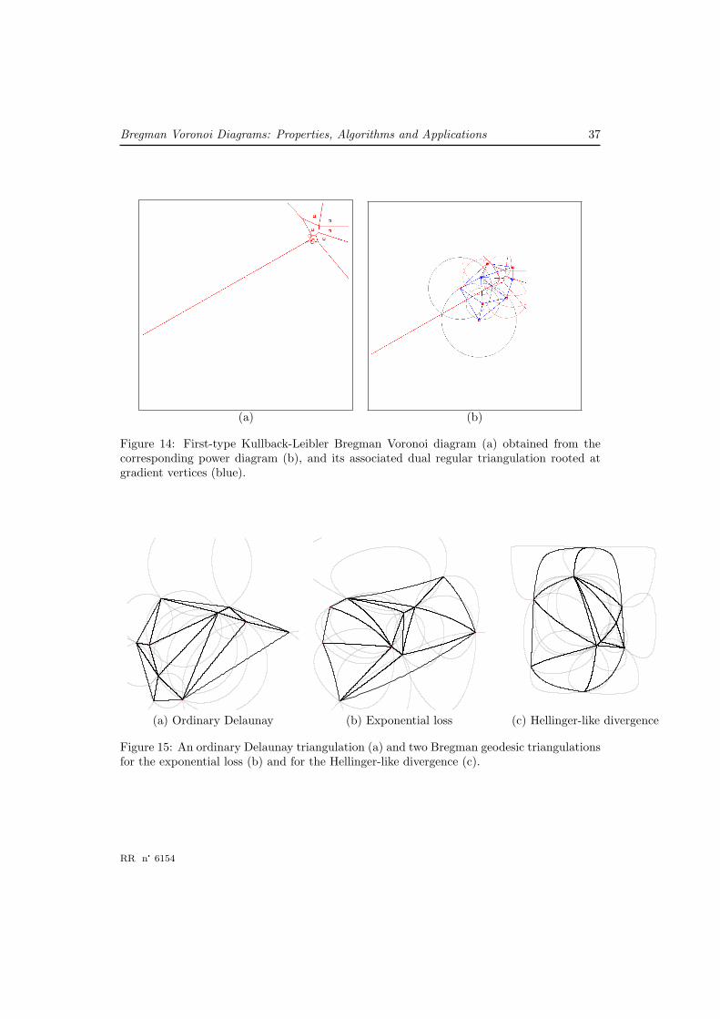
Figure 14: First-type Kullback-Leibler Bregman Voronoi diagram (a) obtained from thecorresponding power diagram (b), and its associated dual regular triangulation rooted atgradient vertices (blue).

(a) Ordinary Delaunay (b) Exponential loss (c) Hellinger-like divergence

Figure 15: An ordinary Delaunay triangulation (a) and two Bregman geodesic triangulationsfor the exponential loss (b) and for the Hellinger-like divergence (c).

RR n° 6154


6 Applications

In this section, we give some applications related to computational geometry and machinelearning.

6.1 Centroidal Bregman Voronoi diagrams and Lloyd quantization

Let D be a domain of X and p(x) be a density function defined over D. We define theBregman centroid of D as the point c∗ ∈ D such that c∗ = argminc∈D

∫x∈D p(x)DF (x||c) dx.

The following lemma states that the mass Bregman centroid of D is uniquely defined andindependent of F .

Lemma 11 The Bregman centroid of D coincides with the mass centroid of D.

Proof:

∇c

∫x∈D

p(x) DF (x||c) dx = ∇c

∫x∈D

p(x) (F (x)− F (c)− 〈x− c,∇F (c)〉)dx

= −∫x∈D

p(x) ∇2F (c)(x− c)dx

= −∇2F (c)(∫x∈D

p(x) xdx− c∫x∈D

p(x) dx).

Hence, c∗ =Rx∈D p(x) xdxRx∈D p(x) dx

. �

When x is a random variable following the probability density p(x),∫x∈D p(x) DF (x||c) dx is called the distortion rate associated to the representative c,

the optimal distortion-rate function∫x∈D p(x) DF (x||c∗) dx is called the Bregman informa-

tion, and c∗ is called the Bregman representative. The above result states that the optimaldistortion rate exists and does not depend on the choice of the Bregman divergence, andthat the Bregman representative c∗ is the expectation E(x) of x. This result extends ananalogous result in the discrete case (finite point sets) studied in [6].

Computing a centroidal Bregman Voronoi diagram of k points can be done by means ofLloyd’s algorithm [30]. We select an initial set of k points. Then, we iteratively compute aBregman Voronoi diagram and move the sites to the Bregman centroids of the correspondingcells in the diagram. Upon convergence, the output of the algorithm is a local minimizerof f((pi, Vi), i = 1, . . . , k) =

∑ki=1

∫x∈Vi

DF (x||pi) dx , where {pi}ki=1 denotes any set of k

points of X and {Vi}ki=1 denotes any tesselation of X into k regions. See [18] for a further

discussion and applications of centroidal Voronoi diagrams.

6.2 ε-nets

Lloyd’s algorithm intends to find a best set of k points for a given k so as to minimize aleast-square criterion. Differently, we may want to sample a compact domain D ⊂ X up to a

INRIA


given precision while minimizing the number of samples. Instead of a least-square criterion,we define the error associated to a sample P as error(P ) = maxx∈D minpi∈P DF (x||pi). Afinite set of points P of D is an ε-sample of D iff error(P ) ≤ ε.

An ε-sample P is called an ε-net if it satisfies the sparsity condition:max(DF (p||q), DF (q||p)) > ε for any two points p and q in P .

We will see how to construct an ε-net. For simplicity, we assume in the rest of the sectionthat D is a convex polytope. Extending the results to more general domains is possible.

Let P ⊂ D, vorF (P ) be the Bregman Voronoi diagram of P and vorF |D(P ) be itsrestriction to D. Write V for the set of vertices of vorF |D(P ). V consists of vertices ofvorF (P ) and intersection points between the edges of vorF (P ) and the boundary of D. Thefollowing lemma states that error(P ) can be computed by examining only a finite numberof points, namely the points of V .

Lemma 12 error(P ) = maxv∈V minpi∈P DF (x||pi).

Proof: Let x ∈ D, px the point of P closest to x and Vx the associated cell of vorF |D(P )(which contains x). Vx is a bounded polytope whose vertices belongs to V . Let w be thevertex of Vx most distant from px. We have DF (x||px) ≤ DF (w||px). This is a consequenceof the convexity of F and of the fact that DF (x||p) is measured by the vertical distancebetween x and Hp (Lemma 1). �

An ε-net of D can be constructed by the following greedy algorithm originally proposedby Ruppert in the context of mesh generation [39]. See also [20]. We initialize the sampleset P0 with d points of D lying at distance greater than ε from one another. Then, ateach step, the algorithm looks for the point vi of D that is the furthest (for the consideredBregman divergence) from the current set of samples Pi. By Lemma 12, this step reducesto looking at the vertices of vorF |D(Pi). If DF (x||vi) ≤ ε, the algorithm stops. Otherwise,we take vi as a new sample point, i.e. pi+1 = vi, we update the set of sample points, i.e.Pi+1 = Pi ∪ {pi+1}, and insert pi+1 in the Bregman Voronoi diagram of the sample points.Upon termination, the set of sample points Pt satisfies the hypothesis of Lemma 12 andtherefore Pt is an ε-sample of D. Moreover, for any two points p and q of Pt, we haveDF (p||q) > ε or DF (q||p) > ε, depending on whether p has been inserted after or before q.Indeed, we only insert a point if its divergence to the points of the current sample is greaterthan ε. Hence, Pt is an ε-net of D.

To prove that the algorithm terminates, we need the following lemma. Given a Bregmanball B(c, r), we define the biggest Euclidean ball EB(c, r′) contained in B(c, r) and thesmallest Euclidean ball EB(c, r′′) containing B(c, r).

Lemma 13 Let F be a strictly convex function of class C2, there are constants γ′ and γ′′

(that do not depend on c nor on r) such that r′2 ≥ γ′r and r′′2 ≤ γ′′r.

Proof: According to Taylor’s formula, there exists a point t of the open segment xc suchthat

F (x) = F (c) + 〈x− c,∇F (c)〉+12

(x− c)T ∇2F (t)(x− c).

RR n° 6154


Hence,

DF (x||c) = F (x)− F (c)− 〈x− c, c′〉 =12

(x− c)T ∇2F (t)(x− c), (14)

where t is a point of the open segment xc.Since F is strictly convex, the Hessian matrix is positive definite (i.e., xT ∇2F (t)x > 0

for all x in X ), and the domain D being compact, there exist two constants η′ and η′′ suchthat, for any y ∈ D, 0 < η′′ ≤ ||∇2F (y)|| ≤ η′. If ‖x− c‖2 > 2r

η′′ (Frobenius matrix norm),

we deduce from Equation (14) that DF (x||c) > r. Therefore, B(c, r) ⊂ EB(c,√

2rη′′ ).

If ‖x− c‖2 ≤ 2rη′ , we have using again Equation (14)

DF (x||c) ≤ η′

2‖x− c‖2 ≤ r.

Therefore, EB(c,√

2rη′ ) ⊂ B(c, r). �

Let p and q be two points such that DF (p||q) = r. Observing that EB(p, r′) ⊆EB(p, ‖p− q‖) ⊆ EB(p, r′′), we deduce from the above lemma that√

γ′ r ≤ ‖p− q‖ ≤√

γ′′ r (15)

andγ′

γ′′DF (p||q) ≤ DF (q||p) ≤ γ′′

γ′DF (p||q).

Another consequence of the lemma is that the volume of any Bregman ball of radius atleast r > 0, is bounded away from 0 (when F is of class C2). Hence, since D is compact,the algorithm cannot insert infinitely many points and therefore terminates. Moreover, thesize of the sample output by the algorithm can be bounded, as stated in the next lemma.Write D≤ε = {x| ∃y ∈ D, ‖x− y‖ ≤ ε}.

Lemma 14 If F is of class C2, the algorithm terminates. If Pt denotes the final set ofsample points, we have |Pt| = O

(vol(D)εd/2

).

Proof: We have already shown that the algorithm terminates. Let Pt be the set of pointsthat have been inserted by the algorithm, excluding the initial set (of constant size). Letτ(x) = inf{r : |EB(x, r)

⋂Pt| ≥ 2} and Bp = EB(p, τ(p)

2 ), p ∈ Pt. It is easy to see that τis 1-Lipschitz and that the Euclidean balls Bp, p ∈ Pt are disjoint. Let q be a point of Pt

closest to p : τ(p) = ‖p− q‖ and, as noticed above, max(DF (p||q), DF (q||p)) > ε. Eq. 15then implies that τ(p) = ‖p − q‖ ≥

√γ′ ε. Consider now the midpoint m of pq and write

t for the point of Pt that minimizes DF (m||.). Since D is convex, m ∈ D and, according tothe definition of q, ‖m − p‖ ≤ ‖m − t‖. Eq. 15 and the fact that Pt is an ε-sample of Dthen yield ‖m− t‖ ≤

√γ′′ ε. In summary, we have√

γ′ ε ≤ τ(p) = ‖p− q‖ ≤ 2√

γ′′ ε. (16)

INRIA


The right inequality shows that all the balls Bp, p ∈ Pt, are contained in D≤η whereη =

√γ′′ ε. We can now bound the size of Pt.∫

D≤ηdx

τd(x)≥

∑p∈Pt

∫Bp∩D≤η

dxτd(x)

(the balls Bp have disjoint interiors)

≥∑

p∈Pvol(Bp∩D≤η)

( 32 τ(p))d (τ(x) ≤ τ(p) + ‖p− x‖ ≤ 3

2τ(p))

≥ C3d |Pt|

where C = πp

p! if d = 2p and C = 22p−1(p−1)! πp−1

(2p−1)! if d = 2p− 1.Using again the Lipschitz property of τ and Eq 16, we have for all x ∈ Bp

τ(x) ≥ τ(p)− ‖x− p‖ ≥ 12

τ(p) ≥ 12

√γ′ ε

We deduce

|Pt| ≤(

6√γ′

)d 1Cεd/2

∫D≤η

dx.

�A geometric object O is said α-fat [7] if the ratio r+

r− of the radius r+ of the smallestball enclosing O over the radius r− of the largest ball inscribed in O is bounded by α:r+

r− ≤ α. Euclidean balls are therefore 1-fat, namely the fattest objects. It has been shownthat considering the fatness factor for a set of objects yields in practice efficient tailoreddata-sensitive algorithms [7] by avoiding bad configurations of sets of skinny objects. Adirect consequence of Lemma 13 is that Bregman balls (in fixed dimensions) are fat (i.e.,α = O(1)) on any compact domain:

Corollary 3 For C2 Bregman generator functions, Bregman balls on any compact domainare fat.

Proof: Indeed, consider any Bregman ball defined on a compact domain for a C2 strictlyconvex and differentiable Bregman generator function F . Its fatness α is upper bounded by√

γ′

γ′′ , where γ′ and γ′′ are the two constants (depending on F and D) of Lemma 13. Recallthat Lemma 13 considers concentric Euclidean balls ham sandwiching a Bregman ball, allcentered at position c. We have α ≤ r+

r− ≤ r+

r−c≤ r+

c

r−c= O(1) since r−c ≤ r− and r+

c ≥ r+,where r+

c (respectively, r−c ) denote the radius of the smallest enclosing (respectively, largestinscribed) Euclidean ball centered at c. The fatness property simply means that we cancover any Bregman ball by a constant number of (convex) Euclidean balls. �

Thus, since Bregman balls are fat on compact domains, we can build efficient data-structures for point location with applications to piercing (geometric 0-transversal) andothers, as described in [19].

RR n° 6154


6.3 VC-dimension, classification and learning

Some important classification rules rely on Voronoi diagrams; furthermore, the analysis ofclassification rules (complexity or statistical generalization) sometimes makes use of conceptsclosely related to Voronoi diagrams. Extending the rules and analyses to arbitrary Bregmandivergences, with important related consequences (such as the eventual lost of convexity) isthus particularly interesting for classification, and we review here some notable consequences.

In supervised classification, we are generally interested in capturing the joint structure ofX and a set of classes, {0, 1} in the simplest case. For this objective, we build representationsof concepts, i.e. functions that map X to the set of classes. A concept class H is a set ofconcept representations h : X → {0, 1}; for example, should h be a Bregman ball, it wouldclassify 0 the points outside the ball, and 1 the points inside. Armed with these definitions,our supervised classification problem becomes the following one. A so-called target concept,c, which is unknown, labels the points of X ; we have access to its labeling throughout asampling process: we retrieve examples (i.e., pairs (x, c(x))), independently at random,according to some unknown but fixed distribution D over the set {(x, c(x)) : x ∈ X}. Thequestion is: what are the conditions on H that guarantee the possibility to build, withinreasonable time, some h ∈ H agreeing as best as possible with c, with high probability?While the complexity requirement is usual in computer science, the fact that we requireadequacy with high probability better than systematically is also a necessary requirement,as there is always the possibility of an extremely bad sampling that would prevent anyefficient learning (e.g. we have drawn the same example all the time). In general, ratherthan directly sampling the domain, we work with a finite data set S of examples which issupposed to be sampled this way.

From the statistical standpoint, learning requires to find a good balance between theaccuracy, i.e. the goodness-of-fit of h as measured on S, and the capacity ofH, i.e. its abilityto learn (or fit in generalization) the data with the smallest number of errors. Consider forexample geometric figures in the plane and the “square” concept. Intuitively, an H with toolarge capacity is like the person who picks a huge quantity of geometric figures includingsquares, memorizes each of them, and then rejects every square that would not exactly be inits collection (edge lengths, colors, etc.). An H with too little capacity is like the lazy personwho keeps as sole concept the fact that squares have four edges. Both extremal situationsmean little generalization capabilities, but for different reasons.

There have been intensive lines of works on the measures of this capacity, and one ofthe most popular is the VC-dimension [17]. Informally, the VC-dimension of H is the sizeof the largest dataset S for which H shatters S, i.e. for which H contains all the classifiersthat could perform any of the 2|S| possible labelings of the data. To be more formal, letΠH(S) = {(h(p1), h(p2), ..., h(pn)) | h ∈ H} denote the set of all distinct tuples of labelson S that can be performed by elements of H. While it always holds that ΠH(n) ≤ 2n, themaximal n for which ΠH(n) = 2n is the VC-dimension of H, VCdim(H). The importance ofthe VC-dimension comes from the fact that it allows to bound the behavior of the empiricaloptimal classifier in a distribution-free manner [17]. In particular, if the VC-dimension isfinite, the average error probability of the empirical optimal classifier tends to 0 when the

INRIA


size of the training data set increases. The following lemma proves that the VC-dimensionof Bregman balls is the same as for linear separators, and this does not depend on the choiceof F .

Theorem 17 The VC dimension of the class of all Bregman balls BF of Rd (for any givenstrictly convex and differentiable function F ) is d + 1.

Proof: We use the lifting map introduced in Section 3.2. Given a set S of points in Rd, welift them onto F , obtaining S ∈ Rd+1.

Let BF be a Bregman ball and write σ for the Bregman sphere bounding BF . FromLemma 5, we know that, for any p ∈ Rd, p ∈ B iff p ∈ H↓

σ. For a given function F , letBF denote the set of all Bregman balls, and let HF denote the set of all lower halfspaces ofRd+1. It follows from the observation above that B shatters S iff H shatters S. Hence theVC dimension of B over the sets of points of Rd is equal to the VC dimension of H over thesets of points of F ⊂ Rd+1.

Since the points of S are in convex position, they are shattered by H iff the affine hullof their convex hull is of dimension strictly less than the dimension of the embedding space,i.e. d+1, which happens iff |S| < d+2. Indeed otherwise, the subset of vertices of any facetof the upper convex hull of S cannot be obtained by intersecting S with a lower halfspace(an upper halfspace would be required). Hence, the VC dimension of Bregman balls is atmost d + 1.

It is exactly d + 1 since any set of d + 1 points on F in general position generates a d-dimensional affine hull A that cannot be shattered by less than d+1 hyperplanes of A. Thesame result plainly holds for hyperplanes of Rd+1 since we can associate to each hyperplaneh of A a hyperplane H of Rd+1 such that h = H ∩ A. �

This result does not fall into the general family of VC bounds for concept classes pa-rameterized by polynomial-based predicates [23], it is mostly exact, and it happens not todepend on the choice of the Bregman divergence. This has a direct consequence for classi-fication, which is all the more important as Bregman balls are not necessarily convex (seeFigure 5). Because the capacity of Bregman balls is not affected by the divergence, if wefit this divergence in order to minimize the empirical risk (risk estimated on S), then thereis an efficient minimization of the true risk (risk estimated on the full domain X ), as well.There is thus little impact (if any) on overfitting, one important pitfall for classification,usually caused by over-capacitating the classifiers by tuning too many parameters.

Some applications of our results in supervised learning also meet one of the oldestclassification rule: the k-Nearest Neighbors (k-NN) rule [22], in which a new observationreceives the majority class among the set of its k nearest neighbors, using e.g. k-orderVoronoi diagrams of S (Section 4.4). Various results establish upperbounds for the k-NNrule that depend on the Bayes risk (the true risk of the best possible rule) [17]. The choiceof the proximity notion between observations (it is often not a metric for complex domains)is crucial: if it is too simple or oversimplified, it degrades the k-NN results and may evendegrade Bayes risk as well; if it is too complicated or complexified, it may degrade the testresults via the capacity of the rule. Searching for accurate “distance” notions has been

RR n° 6154


an active field of research in machine learning in the past decade [42]. Our results on thelinearity of the Bregman Voronoi diagrams essentially show that we can mix arbitraryBregman divergences for heterogenous data (mixing binary, real, integer values, etc.)without losing anything from the capacity standpoint.

Range spaces of finite VC-dimensions have found numerous applications in Combinatorialand Computational Geometry. We refer to Chazelle’s book for an introduction to the subjectand references wherein [15]. In particular, Bronnimann and Goodrich [13] have proposed analmost optimal solution to the disk cover algorithm, i.e. to find a minimum number of disksin a given family that cover a given set of points. Theorem 17 allows to extend this resultto arbitrary Bregman ball cover (see also [21]).

7 Conclusion

We have defined the notion of Bregman Voronoi diagrams and showed how these geometricstructures are a natural extension of ordinary Voronoi diagrams. Bregman Voronoi diagramsshare with their Euclidean analogs surprisingly similar combinatorial and geometric proper-ties. We hope that our results will make Voronoi diagrams and their relatives applicable innew application areas. In particular, Bregman Voronoi diagrams based on various entropicdivergences are expected to find applications in information retrieval (IR), data mining,knowledge discovery in databases, image processing (e.g., see [24]). The study of BregmanVoronoi diagrams raises the question of revisiting computational geometry problems in thisnew light. This may also allow one to tackle uncertainty (’noise’) in computational geometryfor fundamental problems such as surface reconstruction or pattern matching.

A limitation of Bregman Voronoi diagrams is their combinatorial complexity that de-pends exponentially on the dimension. Since many applications are in high dimensionalspaces, building efficient data-structures is a major avenue for further research.

Acknowledgements

Frederic Chazal, David Cohen-Steiner and Mariette Yvinec are gratefully acknowledged fortheir comments on this paper. The work by the second author has been partially supportedby the project GeoTopAl (1555) of the Agence Nationale de la Recherche (ANR).

References

[1] S. Amari and H. Nagaoka. Methods of Information Geometry. Oxford University Press,ISBN 0-8218-0531-2, 2000.

[2] A. Ben-Hur, D. Horn, H. T. Siegelmann, and V. Vapnik Support Vector Clustering.Journal of Machine Learning Research, (2):125-137, 2001.

INRIA


[3] F Aurenhammer. Power diagrams: Properties, algorithms and applications. SIAMJournal of Computing, 16(1):78–96, 1987.

[4] F. Aurenhammer and H. Imai. Geometric relations among voronoi diagrams. In 4thAnnual Symposium on Theoretical Aspects of Computer Sciences (STACS), pp. 53–65,1987.

[5] F. Aurenhammer and R. Klein. Voronoi Diagrams. In J. Sack and G. Urrutia (Eds),Handbook of Computational Geometry, Chapter V, pp. 201–290. Elsevier Science Pub-lishing, 2000.

[6] A. Banerjee, S. Merugu, I. S. Dhillon, and J. Ghosh. Clustering with Bregman diver-gences. Journal of Machine Learning Research (JMLR), 6:1705–1749, 2005.

[7] M. de Berg, M. Katz, F. van der Stappen, and J. Vleugels. Realistic input models forgeometric algorithms. Algorithmica 34:81-97, 2002.

[8] J.-D. Boissonnat and M. Karavelas. On the combinatorial complexity of EuclideanVoronoi cells and convex hulls of d-dimensional spheres. In Proc. 14th ACM-SIAMSympos. Discrete Algorithms (SODA), pp. 305–312, 2003.

[9] J.-D. Boissonnat, C. Wormser, and M. Yvinec. Anisotropic diagrams: Labelle Shewchukapproach revisited. In 17th Canadian Conference on Computational Geometry (CCCG),pp. 266–269, 2005.

[10] J.-D. Boissonnat and M. Yvinec. Algorithmic Geometry. Cambridge University Press,New York, NY, USA, 1998.

[11] J.-D. Boissonnat, C. Wormser, and M. Yvinec. Curved Voronoi diagrams. In J.-D.Boissonnat and M. Teillaud (Eds) Effective Computational Geometry for Curves andSurfaces, pp. 67–116. Springer-Verlag, Mathematics and Visualization, 2007.

[12] L. M. Bregman. The relaxation method of finding the common point of convex setsand its application to the solution of problems in convex programming. USSR Compu-tational Mathematics and Mathematical Physics, 7:200–217, 1967.

[13] H. Bronnimann and M. T. Goodrich. Optimal set covers in finite VC-dimension. Dis-crete & Computational Geometry, 14(4):463–479, 1995.

[14] B. Chazelle. An optimal convex hull algorithm in any fixed dimension. Discrete Com-putational Geometry, 10:377–409, 1993.

[15] B. Chazelle. The Discrepancy Method. Cambridge University Press, Cambridge, U.K.,2000.

[16] I. Csiszar. Why least squares and maximum entropy? An axiomatic approach toinference for linear inverse problems. Ann. Stat., 19:2032–2066, 1991.

RR n° 6154


[17] L. Devroye, L. Gyorfi, and G. Lugosi. A Probabilistic Theory of Pattern Recognition.Springer, 1996.

[18] Q. Du, V. Faber, and M. Gunzburger. Centroidal Voronoi tesselations: Applicationsand algorithms. SIAM Review, 41:637–676, 1999.

[19] A. Efrat, M. J. Katz, F. Nielsen, and M. Sharir. Dynamic data structures for fat objectsand their applications. Comput. Geom. Theory Appl., 15(4):215–227, 2000.

[20] Y. Eldar, M. Lindenbaum, M. Porat, and Y. Y. Zeevi. The farthest point strategy forprogressive image sampling. IEEE Trans. on Image Processing, 6(9):1305–1315, 1997.

[21] G. Even, D. Rawitz, and S. Shahar. Hitting sets when the VC-dimension is small. Inf.Process. Lett., 95(2):358–362, 2005.

[22] E. Fix and J. L. Hodges. Discrimatory analysis, nonparametric discrimination. Techni-cal Report TR-21-49-004, Rept 4, USAF School of Aviation Medicine, Randolph Field,TX, 1951.

[23] P.-W. Goldberg and M. Jerrum. Bounding the Vapnik-Chervonenkis dimension ofconcept classes parameterized by real numbers. Machine Learning, 18:131–148, 1995.

[24] M. Inaba and H. Imai. Geometric clustering models for multimedia databases. InProceedings of the 10th Canadian Conference on Computational Geometry (CCCG’98),1998.

[25] M. Inaba and H. Imai. Geometric clustering for multiplicative mixtures of distributionsin exponential families. In Proceedings of the 12th Canadian Conference on Computa-tional Geometry (CCCG’00), 2000.

[26] R. Klein. Concrete and Abstract Voronoi Diagrams, volume 400 of Lecture Notes inComputer Science. Springer, 1989. ISBN 3-540-52055-4.

[27] F. Labelle and J. R. Shewchuk. Anisotropic voronoi diagrams and guaranteed-qualityanisotropic mesh generation. In Proc. 19th Symposium on Computational Geometry(SoCG), pages 191–200, New York, NY, USA, 2003. ACM Press.

[28] J. Lafferty. Additive models, boosting, and inference for generalized divergences. InProc. 12th Conference on Computational learning theory, 125-133, 1999.

[29] D.-D. Le and S. Satoh. Ent-Boost: Boosting Using Entropy Measure for Robust ObjectDetection. In Proc. 18th International Conference on Pattern Recognition, pp. 602-605,2006.

[30] S. P. Lloyd. Least squares quantization in PCM. IEEE Transactions on InformationTheory, 28(2):129–136, 1982.

INRIA


[31] P. McMullen. The maximum numbers of faces of a convex polytope. J. CombinatorialTheory, Ser. B, 10:179–184, 1971.

[32] F. Nielsen. Visual Computing: Geometry, Graphics, and Vision. Charles River Me-dia/Thomson Delmar Learning, ISBN 1584504277, 2005.

[33] M. Teillaud O. Devillers, S. Meiser. The space of spheres, a geometric tool to unifyduality results on voronoi diagrams. Technical Report No.1620, INRIA, 1992.

[34] K. Onishi and H. Imai. Voronoi diagram in statistical parametric space by Kullback-Leibler divergence. In Proc. 13th Symposium on Computational Geometry (SoCG),pages 463–465, New York, NY, USA, 1997. ACM Press.

[35] K. Onishi and H. Imai. Voronoi diagrams for an exponential family of probabilitydistributions in information geometry. In Japan-Korea Joint Workshop on Algorithmsand Computation, 1997.

[36] S. Pion and M. Teillaud. 3d triangulation data structure. In CGAL Editorial Board,editor, CGAL-3.2 User and Reference Manual. 2006.

[37] V. T. Rajan. Optimality of the Delaunay triangulation in Rd. Discrete & ComputationalGeometry, 12:189–202, 1994.

[38] R. T. Rockafellar. Convex Analysis. Princeton University Press, Princeton, New Jersey,1970.

[39] J. Ruppert. A Delaunay refinement algorithm for quality 2-dimensional mesh genera-tion. J. Algorithms, 18:548–585, 1995.

[40] K. Sadakane, H. Imai, K. Onishi, M. Inaba, F. Takeuchi, and K. Imai. Voronoi diagramsby divergences with additive weights. In Proc. 14th Symposium on ComputationalGeometry (SoCG), pages 403–404, New York, NY, USA, 1998. ACM Press.

[41] M. Sharir. Almost tight upper bounds for lower envelopes in higher dimensions. DiscreteComput. Geom., 12:327–345, 1994.

[42] D. Randall Wilson and Tony R. Martinez. Improved heterogeneous distance functions.Journal of Artificial Intelligence Research, 1:1–34, 1997.

RR n° 6154


Contents

1 Introduction and prior work 3

2 Bregman divergences 62.1 Definition and basic properties . . . . . . . . . . . . . . . . . . . . . . . . . . 62.2 Legendre duality . . . . . . . . . . . . . . . . . . . . . . . . . . . . . . . . . . 82.3 Symmetrized Bregman divergences . . . . . . . . . . . . . . . . . . . . . . . . 112.4 Exponential families . . . . . . . . . . . . . . . . . . . . . . . . . . . . . . . . 11

2.4.1 Parametric statistical spaces and exponential families . . . . . . . . . 112.4.2 Kullback-Leibler divergence of exponential families . . . . . . . . . . . 122.4.3 Dual parameterizations and dual divergences . . . . . . . . . . . . . . 14

3 Elements of Bregman geometry 153.1 Bregman bisectors . . . . . . . . . . . . . . . . . . . . . . . . . . . . . . . . . 153.2 Bregman spheres and the lifting map . . . . . . . . . . . . . . . . . . . . . . . 163.3 Projection, orthogonality and geodesics . . . . . . . . . . . . . . . . . . . . . 21

4 Bregman Voronoi diagrams 254.1 Three types of diagrams . . . . . . . . . . . . . . . . . . . . . . . . . . . . . . 254.2 Bregman Voronoi diagrams from polytopes . . . . . . . . . . . . . . . . . . . 274.3 Bregman Voronoi diagrams from power diagrams . . . . . . . . . . . . . . . . 294.4 Generalized Bregman divergences and their Voronoi diagrams . . . . . . . . . 30

5 Bregman triangulations 345.1 Bregman Delaunay triangulations . . . . . . . . . . . . . . . . . . . . . . . . . 345.2 Bregman geodesic triangulations . . . . . . . . . . . . . . . . . . . . . . . . . 36

6 Applications 386.1 Centroidal Bregman Voronoi diagrams and Lloyd quantization . . . . . . . . 386.2 ε-nets . . . . . . . . . . . . . . . . . . . . . . . . . . . . . . . . . . . . . . . . 386.3 VC-dimension, classification and learning . . . . . . . . . . . . . . . . . . . . 42

7 Conclusion 44

INRIA

Unité de recherche INRIA Sophia Antipolis2004, route des Lucioles - BP 93 - 06902 Sophia Antipolis Cedex (France)

Unité de recherche INRIA Futurs : Parc Club Orsay Université - ZAC des Vignes4, rue Jacques Monod - 91893 ORSAY Cedex (France)

Unité de recherche INRIA Lorraine : LORIA, Technopôle de Nancy-Brabois - Campus scientifique615, rue du Jardin Botanique - BP 101 - 54602 Villers-lès-Nancy Cedex (France)

Unité de recherche INRIA Rennes : IRISA, Campus universitaire de Beaulieu - 35042 Rennes Cedex (France)Unité de recherche INRIA Rhône-Alpes : 655, avenue de l’Europe - 38334 Montbonnot Saint-Ismier (France)

Unité de recherche INRIA Rocquencourt : Domaine de Voluceau - Rocquencourt - BP 105 - 78153 Le Chesnay Cedex (France)

ÉditeurINRIA - Domaine de Voluceau - Rocquencourt, BP 105 - 78153 Le Chesnay Cedex (France)

http://www.inria.fr

ISSN 0249-6399

bregman voronoi diagrams: properties, algorithms and

Documents