brenno castrillon menezes - epqb.eq.ufrj.brepqb.eq.ufrj.br/download/quantitative-methods-for... ·...

1

UNIVERSIDADE FEDERAL DO RIO DE JANEIRO

ESCOLA DE QUÍMICA

BRENNO CASTRILLON MENEZES

DOCTORATE EXAM

QUANTITATIVE METHODS FOR STRATEGIC INVESTMENT PLANNING

IN THE OIL-REFINING INDUSTRY

Advisers:

Prof. Ricardo de Andrade Medronho, TPQB/EQ/UFRJ

Prof. Fernando Pellegrini Pessoa, TPQB/EQ/UFRJ

Co-Adviser:

Eng. Lincoln Fernando Lautenschlager Moro, AB-RE/TR/PR/PETROBRAS

August, 2014

i i

Brenno Castrillon Menezes

QUANTITATIVE METHODS FOR STRATEGIC INVESTMENT PLANNING IN

THE OIL-REFINING INDUSTRY

Tese de Doutorado apresentada ao Programa

em Tecnologia de Processos Químicos e

Bioquímicos, Escola de Química,

Universidade Federal do Rio de Janeiro, como

requisito parcial à obtenção do título de

Doutor em Tecnologia de Proc Químicos e

Bioquímicos.

Advisers:

Prof. Ricardo de Andrade Medronho, TPQB/EQ/UFRJ

Prof. Fernando Pellegrini Pessoa, TPQB/EQ/UFRJ

Co-Adviser:

Eng. Lincoln Fernando Lautenschlager Moro, AB-RE/TR/PR PETROBRAS

Rio de Janeiro

2014

i i i

FICHA CATALOGRÁFICA

Menezes, Brenno Castrillon.

Quantitative methods for strategic investment planning in the oil-refining industry

Brenno Castrillon Menezes. – 2014.

xviii, 183 f.: 51 il.

Tese (Doutorado em Tecnologia de Processos Químicos e Bioquímicos) –

Universidade Federal do Rio de Janeiro, Escola de Química, Rio de Janeiro,

2014.

Orientadores: Ricardo Andrade Medronho, Fernando Luiz Pellegrini Pessoa, Lincoln

Fernando L. Moro.

1. Strategic Planning. 2. Capital Investment Planning. 3. Process Design Synthesis. 4.

Oil-Refining Industry. 5. Capacity Expansion. 6. Net Present Value. 7. Quantitative

Methods. 8. Brazilian Oil-Refining Investments. I. Medronho, Ricardo A.; Pessoa,

Fernando L. P.; Moro, Lincoln F .L. II. Universidade Federal do Rio de Janeiro, Escola de

Química. III. Título.

i v

Brenno Castrillon Menezes

QUANTITATIVE METHODS FOR STRATEGIC INVESTMENT PLANNING IN

THE OIL-REFINING INDUSTRY

Tese de Doutorado apresentada ao Programa

em Tecnologia de Processos Químicos e

Bioquímicos, Escola de Química,

Universidade Federal do Rio de Janeiro, como

requisito parcial à obtenção do título de

Doutor em Tecnologia de Proc Químicos e

Bioquímicos.

Aprovada em

__________________________________________

Prof. Ricardo de Andrade Medronho, Ph.D., EQ/UFRJ (orientador)

__________________________________________

Prof. Fernando Luiz Pellegrini Pessoa, D.Sc., EQ/UFRJ (orientador)

__________________________________________

Lincoln Fernando Lautenschlager Moro, D.Sc., PETROBRAS/AB-RE (orientador)

__________________________________________

Prof. Eduardo Mach Queiroz, D.Sc., EQ/UFRJ

__________________________________________

Fabio dos Santos Liporace, D.Sc., PETROBRAS/CENPES

__________________________________________

Prof. Jose Vitor Bomtempo, D. Sc., EQ/UFRJ

__________________________________________

Marcel Joly, D.Sc., PETROBRAS/RECAP

__________________________________________

Marcus Vinicius Oliveira Magalhães, Ph.D., PETROBRAS/AB-PQ

v

Acknowledgements

First and foremost, I would like to thank Professors Ricardo de Andrade Medronho and

Fernando Pellegrini Pessoa for being my advisors. As well as my colleague and co-adviser

Lincoln Fernando L Moro.

At the same time, I would like to thank my committee members – Marcus Vinicius

Magalhaes, Marcel Joly, Fabio Liporace, Jose Vitor Bomtempo and Eduardo March for their

valuable feedback and the effort they spent in evaluating this work.

I had the pleasure to work with very supportive collaborators from Industrial Algorithms,

Jeffrey Kelly and Alkis Vazacopoulos, who I would like to thank for freed me their Industrial

Modeling & Programming Language (IMPL) software.

Special thanks to Professor Ignacio Grossmann and Jeffrey Kelly for their valuable advices

and their insightful feedback.

I would also like to thank my friends for just being there whenever I needed them: Humberto

Mandaro, Andre Assaf, Whei Oh Lin.

Most importantly, I would like to thank my love and my parents, Rosangela and Gilberto (in

memoriam), and my brother Brunno for their love and continuous support.

Finally, I would like to thank PETROBRAS for financial support.

v i

MENEZES, Brenno Castrillon. Quantitative Methods for Strategic Investment Planning

in the Oil-Refining Industry. Rio de Janeiro, 2014. Tese (Doutorado em Tecnologia de

Processos Químicos e Bioquímicos – Escola de Química, Universidade Federal do Rio de

Janeiro, Rio de Janeiro, 2014.

ABSTRACT

Although investment optimization in crude oil-refining can be difficult to handle in a

quantitative manner, the large amount of financial capital involved and the hydrocarbon

processing and logistics complexity force the constant development of high performance

strategic planning methodologies, thus reducing structural bottlenecks and idling in capacity

and capability of equipment within tactical and operational decision-making levels. Besides,

the today’s narrow oil refining margin has further increased the need to improve the

expansion, extension or installation of equipment within a framework of multiperiod and

multisite to guarantee the sustainability of oil refining companies. Unlike traditional process

design scenario- or simulation-based methodologies to construct complex oil-refinery

processing framework, discrete optimization approaches are proposed in this work to solve

the capital investment planning problem also known as assets or facilities planning. The unit

capacity increments (expansion or installation) per type of oil-refinery unit are predicted over

time considering resources such as capital and raw/intermediate material, processing and

blending capabilities, market demands, and project constraints. The strategic investment

model is integrated with the operational model from where hydrocarbon processing and

blending nonlinearities can give rise to non-convex mixed integer nonlinear problems if a full

space model is solved for the strategic and the operational levels simultaneously. Different

modeling strategies to tackle the large scale and complex oil-refining assets expansion

problem are addressed such as (i) the multisite aggregate capacity approach, (ii) the

generalized capital investment planning (GCIP) model with project stages using sequence-

dependent changeover concepts from production scheduling, and (iii) the phenomenological

decomposition heuristic (PDH) to separate the integer/discrete and nonlinear variables. In

terms of oil processing, two new distillation methods in a planning and scheduling

environment are proposed. The first is an improved swing-cut modeling, which uses an

interfacial property-based linear interpolation to predict quality corrections for the light

(upper) and heavy (lower) swing-cut streams using the crude-oil assay distribution curves in

pseudocomponents, hypotheticals or micro-cuts discretized into 10ºC increments for example.

The second is the distillation curve adjustment or shifting modeling to optimize distillate

v i i

stream temperature cutpoints using monotonic interpolation. As cases of studying, this work

analyzes the Brazilian fuel market and the chosen strategies in the recent cycle of expansion

of the national oil-refining assets and proposes different investment portfolio to supply all

market needs within this decade. To demonstrate the effectiveness of the proposed models,

several industrial and Brazilian actual data are provided throughout the work.

Keywords: Strategic Planning, Capital Investment Planning, Capacity Planning, Oil-Refining

Industry, Brazilian Fuel Market, Process Synthesis Design, Quantitative Methods.

v i i i

MENEZES, Brenno Castrillon. Quantitative Methods for Strategic Investment

Planning in the Oil-Refining Industry. Rio de Janeiro, 2014. Tese (Doutorado em

Tecnologia de Processos Químicos e Bioquímicos – Escola de Química, Universidade Federal

do Rio de Janeiro, Rio de Janeiro, 2014.

RESUMO

Embora a otimização de investimentos no refino de petróleo seja difícil de tratar de

modo quantitativo, a grande soma de capital financeiro envolvido e complexidade de

processamento e logística de hidrocarbonetos forçam o constante desenvolvimento de

modelos estratégicos de alta eficiência, reduzindo, portanto, gargalos e inatividades estruturais

na capacidade e habilidade dos equipamentos nos níveis de tomada de decisão táctico e

operacional. Além disso, hoje, a reduzida margem de refino aumentou ainda mais a

necessidade de melhoria do planejamento da expansão, extensão ou instalação de

equipamentos em múltiplos períodos de tempo e múltiplas plantas para garantir a

sustentabilidade das empresas de refino de petróleo. Diferente das tradicionais metodologias

baseadas em cenários ou simulação de esquemas de produção para construir a complexa

estrutura de refino de petróleo, modelos de otimização discreta são propostos neste trabalho

para resolver o problema de planejamento de investimento de capital também conhecido

como planejamento de ativos ou de instalações. Incrementos na capacidade (expansão ou

instalação) por tipo de unidade de processo são encontrados ao longo do tempo considerando

recursos como capital, matéria-prima e insumos, transformações de processamento e mistura,

demandas de mercado e restrições de projeto. O modelo estratégico de investimento é

integrado com o modelo operacional cujas não linearidades do processamento e mistura de

hidrocarbonetos podem levar a problemas misto-inteiros não lineares se o modelo completo é

resolvido para os níveis estratégico e operacional simultaneamente. Diferentes estratégias de

modelagem para lidar com a grande escala e complexidade do problema de expansão de

ativos de refino de petróleo são introduzidos como (i) o modelo de capacidade agregada de

múltiplas plantas, (ii) o modelo genérico para planejamento de investimentos de capital

(GCIP) incluindo estágio dos projetos usando conceitos de transição e sequência dependentes

da programação da produção, e (iii) a heurística de decomposição fenomenológica (PDH)

para separar as variáveis inteiras/discretas e não lineares. Em termos de processamento de

petróleo, dois novos métodos de destilação em ambiente de planejamento e programação da

produção são propostos. O primeiro é o modelo swing-cut (“corte balançante”) aprimorado, o

qual usa uma interpolação linear interfacial baseada na propriedade para prever correções na

i x

qualidade das correntes leve (de cima) e pesada (de baixo) do swing-cut usando curvas de

distribuição do petróleo em pseudo-componentes, hypotheticals ou micro-cortes (micro-cuts)

segmentados a cada 10ºC. O segundo é a modelagem do ajuste ou deslocamento da curva de

destilação para otimizar temperaturas de cortes de correntes destiladas usando interpolação

monotônica. Como casos de estudos, este trabalho analisa o mercado de combustíveis

brasileiro e as estratégias escolhidas no recente ciclo de expansão dos ativos de refino

nacional e propõe diferente portfólio de investimento para suprir todas as necessidades de

mercado dentro desta década. Para demostrar a efetividade dos modelos propostos, vários

dados reais do Brasil e da indústria são fornecidos ao longo do trabalho.

Palavras-Chave: Planejamento Estratégico, Planejamento de Investimento de Capital,

Planejamento de Capacidade, Indústria de Refino de Petróleo, Mercado de Combustíveis

Brasileiro, Síntese de Esquemas de Produção, Métodos Quantitativos.

x

INDEX

1. Introduction ....................................................................................................................................................... 1

1.1. Strategic, Tactical, and Operational Decision-Making Levels Structure in the Oil-Refining Industry ..... 2

1.1.1. Current strategic investment planning structure in PETROBRAS ................................................ 7

1.1.2. Proposed strategic investment planning structure in PETROBRAS .............................................. 8

1.2. Thesis Outline ........................................................................................................................................... 9

1.2.1. Chapter 2 ...................................................................................................................................... 11

1.2.2. Chapter 3 ...................................................................................................................................... 11

1.2.3. Chapter 4 ...................................................................................................................................... 12

1.2.4. Chapter 5 ...................................................................................................................................... 12

1.2.5. Chapter 6 ...................................................................................................................................... 12

1.2.6. Chapter 7 ...................................................................................................................................... 13

1.2.7. Chapter 8 ...................................................................................................................................... 13

1.2.8. Chapter 9 ...................................................................................................................................... 13

2. Bibliographic Review ...................................................................................................................................... 15

2.1. Mathematical Programming Review ....................................................................................................... 15

2.1.1. Modeling Platforms ..................................................................................................................... 15

2.1.2. Types of models and solutions ..................................................................................................... 17

LP and MILP ............................................................................................................... 18 2.1.2.1.

NLP and MINLP ......................................................................................................... 19 2.1.2.2.

2.2. Capital investment planning approaches within the process industry ..................................................... 21

2.3. Distillation models in planning and scheduling environment ................................................................. 24

2.4. Types of models from the thesis ............................................................................................................. 26

3. NLP Production Planning of Oil-Refinery Units for the Future Fuel Market in Brazil: Process Design

Scenario-Based Model ..................................................................................................................................... 28

3.1. Introduction ............................................................................................................................................. 29

3.2. NLP Operational Planning Model ........................................................................................................... 30

3.2.1. Swing-Cut distillation modeling .................................................................................................. 31

3.2.2. Other oil-refinery units ................................................................................................................ 35

3.2.3. Octane number calculation: Ethyl equation ................................................................................. 37

3.3. Problem Statement: The Brazilian Oil Industry Scenario ....................................................................... 38

3.3.1. Fuels demands and production .................................................................................................... 38

3.3.2. Gasoline-Ethanol mix and ethanol for fueling ............................................................................. 39

3.3.3. Future fuels demands ................................................................................................................... 40

3.3.4. Current and planned capacities in 2013, 2016 and 2020 ............................................................. 41

3.3.5. National and imported crude oils ................................................................................................. 41

3.3.6. Crude and fuel prices ................................................................................................................... 43

3.3.7. Crude and fuel quality specifications ........................................................................................... 44

3.3.8. Other relations ............................................................................................................................. 45

3.4. Operational Planning Objective: Daily Operational Profit ...................................................................... 45

3.5. Results and Discussion ............................................................................................................................ 46

3.5.1. Pricing policy in 2013 .................................................................................................................. 47

3.5.2. Conceptual project scenarios in 2020 .......................................................................................... 51

3.5.3. Scenario-based fuel production charts ......................................................................................... 54

3.6. Conclusion .............................................................................................................................................. 56

4. MINLP Production Planning of Oil-Refinery Units for the Future Fuel Market in Brazil: Process Design

Synthesis Model............................................................................................................................................... 58

x i

4.1. Introduction ............................................................................................................................................. 58

4.2. Production Model for Oil-Refinery Units Refit ...................................................................................... 59

4.2.1. MINLP production planning for process design synthesis of oil-refinery units .......................... 59

4.2.2. MILP investment layer for expansion of process units ................................................................ 62

4.3. Problem Statement: The Brazilian Oil-Industry Investment Scenario .................................................... 63

4.3.1. Brazilian oil industry investments after 1997 .............................................................................. 63

4.3.2. Fuel demand scenario tree and investment costs ......................................................................... 65

4.3.3. NPV for expansion of existing units ............................................................................................ 67

4.4. Results and Discussion ............................................................................................................................ 68

4.4.1. NPV-based results from the MINLP process design synthesis problem...................................... 68

4.4.2. Profit- and NPV-based results from the NLP and MINLP production planning problems ......... 74

4.5. Conclusion .............................................................................................................................................. 77

5. Improved Swing-Cut Modeling for Planning and Scheduling of Oil-Refinery Distillation Units ................... 79

5.1. Micro-Cut Crude-Oil Assays and Conventional Swing-Cut Modeling ................................................... 80

5.2. Improved Swing-Cut Modeling .............................................................................................................. 85

5.3. Examples ................................................................................................................................................. 88

5.4. Results ..................................................................................................................................................... 89

5.4.1. Example 1: CDU with three swing-cuts ...................................................................................... 89

5.4.2. Example 2: oil-refinery planning case ......................................................................................... 92

5.5. Conclusions ............................................................................................................................................. 96

6. Distillation Blending and Cutpoint Temperature Optimization using Monotonic Interpolation ..................... 97

6.1. Introduction ............................................................................................................................................. 97

6.2. Distillation Curve Overview ................................................................................................................... 99

6.3. Distillation Blending using Monotonic Interpolation ............................................................................ 103

6.4. Cutpoint Temperature Optimization ..................................................................................................... 105

6.5. Examples ............................................................................................................................................... 108

6.5.1. Example 1: Gasoline blending simulation ................................................................................. 109

6.5.2. Example 2: Diesel blending and cutpoint temperature optimization ......................................... 112

6.5.3. Example 3: Gasoline blending actual versus simulated and optimized ..................................... 114

6.5.4. Example 4: Diesel blending actual versus simulated and optimized ......................................... 116

6.6. Conclusions ........................................................................................................................................... 118

7. Generalized Capital Investment Planning of Oil-Refinery Units using MILP and Sequence-Dependent Setups

...................................................................................................................................................... 120

7.1. Introduction ........................................................................................................................................... 120

7.2. Sequence-dependent setup modeling of stages ..................................................................................... 122

7.2.1. Types of capital investment planning ........................................................................................ 123

7.2.2. Sequence-dependent setup formulation ..................................................................................... 126

7.3. Generalized capital investment planning (GCIP) model using sequence-dependent setups ................. 129

7.3.1. Motivating example 1 ................................................................................................................ 132

7.3.2. Motivating example 2 ................................................................................................................ 134

7.4. Examples ............................................................................................................................................... 136

7.4.1. Retrofit planning of a small process network ............................................................................ 136

7.4.2. Oil-refinery process design synthesis ........................................................................................ 139

7.5. Conclusion ............................................................................................................................................ 141

8. Phenomenological Decomposition Heuristic for Production Synthesis of Oil-Refinery Units ..................... 142

8.1. Introduction ........................................................................................................................................... 142

8.2. Phenomenological decomposition heuristic .......................................................................................... 144

x i i

8.2.1. Partitioning (decomposition) and positioning of models ........................................................... 144

8.2.2. PDH algorithm for oil-refinery design synthesis ....................................................................... 147

8.3. Problem Statement ................................................................................................................................ 149

8.4. Process design synthesis of multisite refineries formulation ................................................................. 153

8.4.1. MILP investment planning model ............................................................................................. 154

8.4.2. Integer constraints for investment .............................................................................................. 156

8.4.3. Integer constraints for framework sequence-dependency .......................................................... 157

8.4.4. NLP operational planning model ............................................................................................... 158

8.5. Results and discussion ........................................................................................................................... 159

8.5.1. Motivating example ................................................................................................................... 159

CCIP modeling results ............................................................................................... 161 8.5.1.1.

GCIP modeling results .............................................................................................. 162 8.5.1.2.

8.5.2. Oil-refinery design synthesis ..................................................................................................... 165

REVAP Investment Planning .................................................................................... 165 8.5.2.1.

São Paulo Supply Chain Refineries Investment Planning ......................................... 166 8.5.2.2.

8.6. Conclusion ............................................................................................................................................ 168

9. Conclusion and Future Work ......................................................................................................................... 169

9.1. Nonlinear Production Planning of Oil-Refinery Units for the Future Fuel Market in Brazil: Process

Design Scenario-Based Model. ............................................................................................................. 169

9.2. Mixed-Integer Nonlinear Production Planning of Oil-Refinery Units for the Future Fuel Market in

Brazil: Process Design Synthesis Model ............................................................................................... 171

9.3. Improved Swing-Cut Modeling for Planning and Scheduling of Oil-Refinery Distillation Units ........ 172

9.4. Distillation Blending and Cutpoint Temperature Optimization using Monotonic Interpolation ........... 173

9.5. A General Approach for Capital Investment Planning using MILP and Sequence-Dependent Setups . 175

9.6. Phenomenological Decomposition Heuristic for Process Design Synthesis of Oil-Refinery Units ...... 177

9.7. Contributions of the Thesis ................................................................................................................... 178

9.8. Recommendations for Future Work ...................................................................................................... 179

9.8.1. Modeling of operational decision-making ................................................................................. 179

9.8.2. Modeling of strategic decision-making ..................................................................................... 181

Appendix A: Investment Strategies for the Future Fuel Market in Brazil ........................................................... 183 Appendix B: Investment costs of oil-refinery units ............................................................................................. 197 Appendix C: IMPL’s configuration and equations formed for the motivating example 1 .................................. 199 Appendix D: Net Present Value Formulation for Investment of Oil-Refinery Units .......................................... 212 Supporting Information ....................................................................................................................................... 216 References ...................................................................................................................................................... 219

x i i i

INDEX OF FIGURES

Figure 1.1. Strategic, tactical and operational decision-making levels within the oil-refining industry. ................. 4

Figure 1.2. Supply chain activities in spatial and temporal dimensions. ................................................................. 5

Figure 1.3. Current strategic investment planning procedure in PETROBRAS. ..................................................... 8

Figure 1.4. Proposed process design synthesis domain for the strategic investment planning modeling in this

work. ........................................................................................................................................................................ 9

Figure 1.5. Overview of the thesis work. ............................................................................................................... 11

Figure 2.1. Three dimensional set of variables in the QLQ problem. .................................................................... 27

Figure 3.1. Oil product deficit of 30% without the refineries in conceptual project phase. .................................. 29

Figure 3.2. Hypothetical refinery REBRA. ........................................................................................................... 31

Figure 3.3. Cut and swing-cut material flow modeling for CDU yields. ............................................................... 33

Figure 3.4. Demand and production levels and forecast considering the 2009-2012 trends. ................................ 38

Figure 3.5. Crude-oil produced, imported and processed and imports and export prices (ANP, 2013). ............... 42

Figure 3.6. National crude-oil production in 2012 (ANP, 2013). .......................................................................... 42

Figure 3.7. Fuels prices percentage (PETROBRAS, 2013b; Agencia T1, 2013). ................................................. 43

Figure 3.8. Initial, intermediate, and final scenarios considered. .......................................................................... 45

Figure 3.9. Demands and production amounts for LPG. ....................................................................................... 54

Figure 3.10. Demands and production amounts for GLNC and GLNCETH. .......................................................... 55

Figure 3.11. Demands and production amounts for jet fuel (JET). ....................................................................... 55

Figure 3.12. Demands and production amounts for diesel (DSL). ........................................................................ 56

Figure 4.1. Investment and operational layers structure. ....................................................................................... 60

Figure 4.2. Investment and operational time periods. ............................................................................................ 60

Figure 4.3. Simulation- and optimization-based approaches to find overall capacity of units. ............................. 61

Figure 4.4. Investments in PETROBRAS after the flexibilization of the market. ................................................. 64

Figure 4.5. Downstream investments per segment in PETROBRAS (PETROBRAS, 2014)................................ 65

Figure 4.6. Four fuel market scenarios in 2016 considered to project the overall refining process scenario in

2020. ...................................................................................................................................................................... 65

Figure 4.7. CDU and VDU plots to find their fixed and variable investment costs. ............................................. 66

Figure 5.1. Example crude-oil assay data with eighty-nine 10ºC micro-cuts for yield, specific gravity and sulfur.

............................................................................................................................................................................... 81

Figure 5.2. Micro-cuts, cuts, swing-cuts and final-cuts. ........................................................................................ 83

Figure 5.3. Multiple crude-oils, cuts and final-cuts for the CDU. ......................................................................... 83

Figure 5.4. Swing-cut properties as a function of light and heavy swing-cut flows. ............................................. 87

Figure 5.5. Specific gravity for each CDU cut including the swing-cuts. ............................................................. 90

Figure 5.6. Sulfur content for each CDU cut including the swing-cuts. ................................................................ 90

Figure 5.7. Fuels production planning case. .......................................................................................................... 93

Figure 6.1. ASTM D86 and TBP volume yield percent curves. .......................................................................... 100

Figure 6.2. Feed and product yield curves. .......................................................................................................... 102

Figure 6.3. Flowchart of distillation blending calculation process. ..................................................................... 105

Figure 6.4. Distillation curve adjustment or shifting, as a function of TBP temperature. ................................... 106

Figure 6.5. Example 1’s LSR interpolated yield (%) versus TBP temperature. .................................................. 110

Figure 6.6. Example 2’s TBP distillation curves, including the final blend. ....................................................... 113

Figure 7.1. Three types of capital investment planning problems. ...................................................................... 124

Figure 7.2. Scheduling stages in a batch process and in our project investment problem. .................................. 128

Figure 7.3. Motivating example 1: small GCIP flowsheet for expansion. ........................................................... 130

Figure 7.4. Gantt chart for expansion of a generalized CIP example. ................................................................. 134

x i v

Figure 7.5. Motivating example 2: small GCIP flowsheet for expansion and installation. ................................. 135

Figure 7.6. Gantt chart for expansion and installation of a generalized CIP example. ........................................ 136

Figure 7.7. Retrofit example for capacity (expansion) and capability (extension) projects. ............................... 137

Figure 7.8. UOPSS flowsheet for Jackson and Grossmann (2002) example. ...................................................... 138

Figure 7.9. Gantt chart for Jackson and Grossmann (2002) example. ................................................................. 139

Figure 7.10. Oil-refinery example flowsheet. ...................................................................................................... 140

Figure 7.11. Gantt chart for the CDU and VDU installations. ............................................................................ 141

Figure 8.1. Partitioning and positioning conjunction variables ........................................................................... 145

Figure 8.2. Two-stage stochastic programming strategy. .................................................................................... 147

Figure 8.3. PDH algorithm flowchart. ................................................................................................................. 148

Figure 8.4. Investment t and operational t0 time-periods. .................................................................................... 150

Figure 8.5. Oil-refinery processing network example. ........................................................................................ 152

Figure 8.6. Material balance in u. ........................................................................................................................ 154

Figure 8.7. Initial and final network for 50 and 15 wwpm S diesel..................................................................... 160

Figure 8.8. Partitioning and positioning GCIP example UOPSS flowsheet. ....................................................... 163

Figure 8.9. Gantt Chart with 1-period and 3-period Past and Future Horizons for the multiperiod MILP. ......... 164

Figure 8.10. São Paulo state supply chain and Brazilian refineries. .................................................................... 165

Figure 9.1. UOPSS scheme. ................................................................................................................................ 176

Figure 9.2. Micro-cuts, hypos (hypothetical species), or pseudocomponents modeling in distillation problems.

............................................................................................................................................................................. 180

Figure 9.3. Strategic, tactical and, operational decision-making levels. .............................................................. 182

Figure A1. Historical and future investments in PETROBRAS (PETROBRAS, 2014a,2014b). ........................ 185

Figure A2. National oil production (ANP, 2013; PETROBRAS, 2013c (forecast)). .......................................... 187

Figure A3. National oil production and national, imported and total oil processed and their ºAPI (ANP, 2013).

............................................................................................................................................................................. 188

Figure A4. Fuel demands and production in the country (ANP, 2013). .............................................................. 189

Figure A5. Diesel grades evolution (MPF, 2013). ............................................................................................... 190

Figure A6. Downstream investment portfolio reevaluation in Brazil (PETROBRAS, 2013a). .......................... 192

Figure A7. Gasoline (GLN) and diesel (DSL) price distribution in Brazil (PETROBRAS, 2014b) and US (US

EIA, 2014). .......................................................................................................................................................... 194

Figure A8. DC and FCC plots to find their fixed and variable investment costs. ............................................... 197

x v

INDEX OF TABLES

Table 2.1. GAMS and IMPL comparison. ............................................................................................................. 17

Table 3.1. Demand forecast for 2016 and 2020. .................................................................................................... 40

Table 3.2. Diesel grades market. ........................................................................................................................... 40

Table 3.3. Overall refining processes capacities for the three production scenarios (k m3/d), excluding lubricant

plants. .................................................................................................................................................................... 41

Table 3.4. Crude oils considered in this work. ...................................................................................................... 43

Table 3.5. Prices (US$/m3) of crude, products, and imports in Brazil grow at a rate 4.2% p.a. ............................ 44

Table 3.6. CDU feed and final products property specifications. .......................................................................... 44

Table 3.7. REBRA profit for the different gasoline and diesel pricing policies. ................................................... 48

Table 3.8. 2013 and 2016 production and market scenarios (thousand cubic meter per day [=] k m3/d). ............. 49

Table 3.9. Actual and calculated data for the current scenario (GLNC) in 2013. ................................................. 49

Table 3.10. Economic and model data for the 2013 and 2016 scenarios. .............................................................. 51

Table 3.11. Production and market scenarios in 2020 (thousand cubic meter per day [=] k m3/d). ...................... 53

Table 3.12. Economic and model data for the 2020 scenarios. ............................................................................. 53

Table 4.1. Fixed and variable investment costs. .................................................................................................... 66

Table 4.2. MINLP problem results for different MINLP and NLP solvers. .......................................................... 70

Table 4.3. NPV value and operational and investment cash flows for the demanded capacity expansion and

investment per type of unit (in billions of U.S. dollars). ....................................................................................... 71

Table 4.4. Daily profit and margin in t1 and t2. ...................................................................................................... 72

Table 4.5. Required capacity (k m3/d) in 2020 to match fuel market demands. .................................................... 73

Table 4.6. Required overall throughput (k m3/d) to match fuel demands at zero crude and fuel imports (except for

LPG and ethanol) in the NLP problem. ................................................................................................................. 75

Table 4.7. Required capacity expansion and investment costs per type of oil-refinery unit to match fuel demands

at zero crude and fuel imports (except for LPG and ethanol) in the NLP problem (values from post-optimization

analysis). ................................................................................................................................................................ 76

Table 4.8. NLP and MINLP results. ...................................................................................................................... 77

Table 5.1. CDU feed and final product specifications. .......................................................................................... 88

Table 5.2. Crude-oil diet with volume compositions. ............................................................................................ 89

Table 5.3. Flows for CDU cuts calculated and the given final-cuts used for both swing-cut methods. ................ 91

Table 5.4. Specific-gravity and sulfur concentration for naphtha to heavy diesel cuts. ........................................ 91

Table 5.5. Specific-gravity and sulfur concentration values for both swing-cut methods. .................................... 92

Table 5.6. Planning example results. ..................................................................................................................... 94

Table 5.7. Cuts flows and properties. .................................................................................................................... 95

Table 5.8. Specific-gravity and sulfur concentration in the CDU feed and final pools. ........................................ 95

Table 5.9. Models sizes. ........................................................................................................................................ 95

Table 5.10. Solvers results. .................................................................................................................................... 95

Table 6.1. Example 1’s Interpolated Evaporation Fraction Results for LSR. ...................................................... 110

Table 6.2. Example 1's Interpolated Evaporation Fraction Results for MCR. ..................................................... 111

Table 6.3. Example 1: Interconverted ASTM D86 (TBP) Temperatures in ºF. .................................................. 111

Table 6.4. Example 1: Statistics. ......................................................................................................................... 112

Table 6.5. Example 2: InterConverted TBP (ASTM D86) Temperatures in ºF................................................... 112

Table 6.6. Example 2: Statistics. ......................................................................................................................... 114

Table 6.7. Example 3: ASTM D86 temperature (ºF), specific gravity, and sulfur content. ................................. 114

Table 6.8. Example 3: Actual, simulated, and optimized properties and specifications. ..................................... 115

Table 6.9. Example 3's actual, simulated, and optimized volumes and prices. ................................................... 115

Table 6.10. Example 3: Statistics. ....................................................................................................................... 116

x v i

Table 6.11. Example 4: ASTM D86 temperatures (ºF), specific gravity, and sulfur content. ............................. 116

Table 6.12. Example 4: Actual, simulated, and optimized volumes and prices. ................................................. 117

Table 6.13. Example 4's actual, simulated and optimized properties and specifications. .................................... 117

Table 6.14. Example 4: Statistics. ....................................................................................................................... 118

Table 8.1. Groups of units to build the superstructure. ........................................................................................ 152

Table 8.2. Motivating example results of the warm-start and the first PDH iteration ......................................... 162

Table 8.3. Motivating example results for the second PDH iteration. ................................................................. 162

Table 8.4. Capacity expansions (exp) and installations (ins) in REVAP............................................................. 166

Table 8.5. REVAP example: Statistics. ............................................................................................................... 166

Table 8.6. Capacity expansions (exp) and installations (ins) in São Paulo refineries. ......................................... 167

Table 8.7. São Paulo refineries example: MILP and NLP Solutions. .................................................................. 167

Table 8.8. São Paulo refineries example: Statistics. ............................................................................................ 168

Table S3.1. Crude-oil assay yields, Ycr,c (%). ...................................................................................................... 216

Table S3.2. Crude-oil assay specific gravity, Gcr,c (g/cm3). ................................................................................. 216

Table S3.3. Crude-oil assay sulfur content, Scr,c (w%). ....................................................................................... 216

Table S3.4. Crude-oil assay acidity, Acr,c (mgKOH/g). ........................................................................................ 216

Table S3.5. Products yields and properties for other oil-refinery units. .............................................................. 217

Table S3.6. Parameter for RON and MON blend values. .................................................................................... 217

Table S8.1. Existing capacity (EXCAP) of the São Paulo refineries. ................................................................. 218

Table S8.2. Demand of the scenario sc=1 (sc=2 is 5% higher and sc=3 is 10%). ............................................... 218

x v i i

LIST OF ACRONYMS

Units

CDU crude distillation unit

CLNHT coker light naphtha hydrotreating

DC delayed coker

DCA delayed coker with atmospheric residue as feed

D1HT diesel hydrotreating (medium severity)

D2HT diesel hydrotreating (high severity)

FCC fluid catalytic cracking

HCC hydrocracking

KHT kerosene hydrotreating

LCNHT light cracked naphtha hydrotreating

PDA propane deasphalting unit

REF reformer

RFCC residue fluid catalytic cracking

ST Stabilizer

VDU vacuum distillation unit

Imports

ETH ethanol

GLNimp gasoline A imported (pure gasoline)

JETimp jet fuel imported

LSDimp light-sulfur diesel imported

LPGimp liquid petroleum gas imported

Products

C1C2 fuel gas (FG)

C3C4 liquid petroleum gas (LPG)

COKE coke

GLN gasoline C (with ethanol)

FG fuel gas

FO fuel oil

H2 hydrogen

HSD high sulfur diesel (1800 wppm S)

JFUEL jet fuel

LGP liquid petroleum gas

LSD low sulfur diesel (10 wppm S)

MSD medium sulfur diesel (500 wppm S)

PQN petrochemical naphtha

USD ultra sulfur diesel (3500 wppm S)

Streams

ASPR asphaltic residue

ATR atmospheric residue

C3 propane

C3= propene

C4 butane

C4= butane

C1C2 fuel gas

x v i i i

C3C4 liquid petroleum gas

CLN coker light naphtha

CLGO coker light gasoil

CHN coker heavy naphtha

CMGO coker medium gasoil

CHGO coker heavy gasoil

DAO deasphalted oil

DO decanted oil

FG fuels gas

FHD final heavy diesel

FK final kerosene

FLD final light diesel

FN final naphtha

FO fuel oil

GLN gasoline

GOST diesel from ST

HCCD hydrocraked diesel

HCCK hydrocraked kerosene

HCCN hydrocraked naphta

HCCO hydrocraked gasoil

HCN heavy cracked naphtha

HD heavy diesel

HNST heavy naphtha from ST

HTCLN hydrotreated coker light naphtha

HTD hydrotreated diesel

HTK hydrotreated kerosene

HTLCN hydrotreated light cracked naphtha

HSD heavy sulfur diesel

HVGO heavy vacuum gasoil

JET jet fuel

K kerosene

LCN light cracked naphtha

LCO light cycle oil

LD light diesel

LNST light naphtha from ST

LSD light sulfur diesel

LVGO light vacuum gasoil

MSD medium sulfur diesel

N naphtha

REFOR reformate

SW1 swing-cut 1

SW2 swing-cut 2

SW3 swing-cut 3

SW1L light swing-cut 1

SW1H heavy swing-cut 1




x i x


VDU vacuum distillation tower

VGO vacuum gasoil

VR vacuum residue

Subscripts

c cuts

cr crude

fc final-cuts

h heavier final-cut

HT hydrotreaters

i,j,m operation mode

imp imports

lighter final-cut

mc micro-cuts

p products

s streams

sw swing-cut

t investment time period

t0 operational time period

u units

Parameters

Acr,c crude assay acidity for each cut

u variable cost for investment in units

u fixed cost for investment in units

CIt capital investment in t

D01 ASTM D86 temperature at 01% evaporation







HT specific gravity reduction in hydrotreaters (not for KHT)

factor to annualize the daily profit

Gcr,c crude assay specific gravity for each cut

Gcr,mc micro-cut specific-gravity (volume-based)

ir interested rate

Mcr,mc micro-cut mass-based property

pr prices

πsc probability of scenario sc

expansion lower bound

expansion upper bound

installation lower bound

installation upper bound

Refcost operational cost

Scr,c crude assay sulfur content for each cut

x x

tr taxes rate

Ycr,c crude assay yield for each cut

Ycr,mc micro-cut volume yield from a crude-oil assay

Ys yields for other oil-refinery unit not CDU/VDU

Vcr,mc micro-cut volume-based property

Variables

Ac cut acidity

Afc final-cut acidity

AROs aromatic concentration of stream s (fixed for some units)

AROV volume-based aromatic concentration

AROVQ quadratic volume-based aromatic concentration

DYNT01 yield delta at 01% evaporation

DYNT99 yield delta at 99% evaporation

Gc cut specific gravity

Gc,fc cut to final-cut specific-gravity property

Gfc final-cut specific gravity

GHT hydrotreaters feed specific gravity (also for units)

Js sensitivity of stream s (fixed for some units)

JV volume-based sensitivity

MONs motor octane number of stream s (fixed for some units)

MONv volume-based motor octane number

MONVv motor octane number blending value

MPc cut mass-based property

MPc,fc cut to final-cut mass-based property

MPfc final-cut property in mass basis

MPIc, interface mass-based property between adjacent lighter cut and cut

MPIc,h interface mass-based property between cut and adjacent heavier cut

NT01 new TBP temperature at 01% evaporation







NY01 normalized yield at 01% evaporation







OT01 old TBP temperature at 01% evaporation





x x i



OLEs olefinic concentration of stream s (fixed for some units)

OLEV volume-based olefinic concentration

Qcr,CDU crude-oil flow to CDU

Qc,fc cut to final-cut flow

Qu’,s,u transfer stream s from u’ to u

QCu,t unit capacity

QEu,t unit expansion in t

QIu,t unit installation in t

QFu unit throughput (also for products)

QFu unit throughput

QSu,s output stream (product) from unit u

RONs research octane number of stream s (fixed for some units)

RONv volume-based research octane number

RONVv motor octane number blending value

Sc cut sulfur content

Sfc final-cut sulfur content

SHT hydrotreater feed sulfur content (also for units)

SHT,s hydrotreater output s (also for units)

VPc cut volume-based property

VPc,fc cut to final-cut volume-based property

VPfc final-cut property in volume basis

VPIc, interface volume-based property between adjacent lighter cut and cut

VPIc,h interface volume-based property between cut and adjacent heavier cut

cr crude diet

yeu,t binary variable to setup the expansion of the unit u in t

yiu,t binary variable to setup the installation of the unit u in t

YNT01 yield at 01% evaporation

YNT99 yield at 99% evaporation

HT severity in hydrotreaters (not for KHT)

Others

HDI heavy diesel interface between HD and SW3-Cut

KLI kerosene interface between SW1-Cut and K

KHI kerosene interface between K and SW2-Cut

LDLI light diesel interface between SW2-Cut and LD

LDHI light diesel interface between LD and SW3-Cut

NI naphtha interface between N and SW1-Cut

1

Chapter 1

1. Introduction

In oil-refining industry, fuels production and crude and fuels distribution can be

optimized in mathematical programming approaches to determine strategic, tactical and

operational settings in supply chains mainly constituted by refinery and terminal sites.

However, in the strategic investment planning optimization to construct oil-refineries or oil

and gas facilities, most methodologies are based on simulation of numerous scenarios, thus

reducing the models to linear (LP) and nonlinear (NLP) problems where the set of material

flows and operating conditions are optimized regarding the selected production and logistics

frameworks.

On the other hand, mixed integer linear (MILP) and mixed integer nonlinear (MINLP)

models are able to optimize discrete decisions such as tasks in scheduling problems and

process design frameworks in strategic investment planning, where the set of process units or

equipment to be invested considering expansion/extension of existing assets and installation

of new ones are set up. To model a full space process design synthesis example by including

continuous and discrete decisions and by taking into account nonlinearities from processing

and blending relations, a non-convex MINLP model arises, in which convergence problems

and model size escalation are the main drawbacks due to limitations in MINLP solvers; hence,

reducing the application of this type of models in industrial-sized problems. Different

strategies or routes to possibly overcome these challenges can be proposed such as

simplification in mathematical formulation, multisite aggregation in capacity, MILP

approximations, warm-start phase to generate initial values, and tailored decomposition

schemes.

The strategic and operational planning approaches to design production scenarios or

frameworks for the oil-refining facilities expansion, extension or installation problem as

proposed in this work deal with more rigorous formulation than those used in general in a

high-level decision-making analysis by considering mixed-integer models, crude dieting,

processing transformations, blending, project staging, and multiperiod and multisite problem.

The need to improve the strategic and tactical decision-making levels in order to address

issues in a quantitative manner rather than the usual qualitative approaches is acknowledged

2

as very relevant by the industry and still remains an active area of research (Shapiro, 2001,

2004).

From the literature on global supply chains, the use of high performance strategic and

tactical supply chain models may result in cost savings within 5–10% (Goetschalckx et al.,

2002). Hence, high performance strategic and tactical models are a paramount towards to the

global supply chain margin improvement that is even more important in the narrow oil

refining margin situation worldwide.

We discuss in section 1.1 the strategic, tactical and operational decision-making levels

structure within the oil-refining industry to introduce the main objectives in each level and

how the strategic investment planning problem is formulated in this work. In section 1.2, the

thesis outline and objectives are presented as well as the current and future thesis related

works in congress and journals (10 in total).

1.1. Strategic, Tactical, and Operational Decision-Making Levels Structure in the Oil-

Refining Industry

In modern process industry, production planning and scheduling better predict

business activities dealing with investment, production, distribution, sales and inventory

within the different decision-making levels (Kallrath, 2002; Grossmann, 2005; Grossmann,

2012). Based on an economic point of view, planning problems deal with high level decisions

such as investment in new facilities, supply chain service and production amounts within the

sites. The main objective is to maximize profit by deducing, from the revenue to be obtained

from products sale, the costs related to raw/intermediate material purchase, investment,

maintenance/turnaround, and manufacturing/logistics operations. On the contrary, in

scheduling problems the cost minimization of tasks is the common objective given that

material resources (raw, inputs, and intermediate streams) and product delivery scenarios are

practically unchanged within the short-term (weeks, days, or hours) or, at least, the material

consumption and production can be held in inventories within a short period of time to

maintain the process despite of changes in premises such as tanks and pipelines inoperability

and delays in deliveries. In scheduling, the disaggregation of structure, time and space, so

different of planning, implies considering lower level decisions such as sequencing of

manufacturing and logistics operations to fulfill a given number of orders or required tasks in

a feasible and if possible optimal scenario, therefore optimizing the performance of the

3

operations. Hence, economics tends to play a greater role in planning than in scheduling

(Grossmann et al., 2002).

Within the process industry decision-making framework, the strategic planning defines

the investments considering the business sustainability in line with future market demands.

The investment portfolio optimization considers the available resources such as raw material,

inputs, plant processing scheme, and capital throughout the operations to supply market

demands. From the strategic decisions up to the product deliveries to clients, the decision

process begins with the strategic choices such investment in production facilities within a

long-term horizon of several years, in which goals are in general defined (without imports,

new refinery for a specific crude oil, etc.). In the medium level, tactical planning considers the

available resources for a mid-term planning (semesters, quarters, months) and gives guidance

to operate corporate decision which are used to define production levels and supply chain

services, all to fulfill in a short-term the operational planning and scheduling decisions among

both production and distribution centers, from a month- to a week-, day-, or an hour-basis.

To increase supply chain productivity and improve business responsiveness there is a

need for efficient integrated approaches to reduce capital and operating costs (Papageorgiou,

2009). This can be achieved by considering hierarchical coordination and collaboration

between the different levels of management (Kelly and Zyngier, 2008). However, there can be

numerous trade-offs between the levels due to their interdependency throughout the supply

chain, so to achieve optimal solutions, ideally, the decisions from the different levels should

be made all together, albeit solution strategies as decomposition may be necessary to solve

industrial-sized models.

Maravelias and Sung (2009) classified the solution strategies for the integrated

planning-scheduling problem into three categories: hierarchical, iterative, and full space.

Although their definition was made for operational planning and scheduling integration, it can

be extended for all decision-making levels. In the hierarchical and iterative strategies it is

implied the need of decomposition methods to solve a master (high-level) problem and a slave

(low-level) problem. The former determines production targets or investment setups as an

input to the latter, in which the details of the operational level either in planning or scheduling

environment are performed. When the information flows only from the master to the slave

problem, the methods are considered hierarchical. If there is a do-loop from the lower-level

back to the master problem as a feedback procedure, then the methods are iterative. As

4

opposed to the decomposed methods, the full-space methods solve the decision-making levels

simultaneously. Figure 1.1 shows the structure of the strategic, tactical, and operational

decision-making levels within the oil-refining industry in which is marked the processing

inside the refineries as a domain of the iteration between the strategic and operational levels

proposed in this work. Optimization within the purchasing and procurement, distribution, and

marketing and sales branches is not being addressed. Instead, the calculation of the strategic

investment analysis are enforced within processing domain, which relies on operational

planning or pre-scheduling snapshots (in cubic meter per day) in order to improve the net

present value accuracy, avoid production inconsistences and smooth the processing-related

uncertainties in the strategic level by better assessing the production.

Figure 1.1. Strategic, tactical and operational decision-making levels within the oil-refining industry.

An optimal strategic formulation capable to incorporate the long-term investments in

line with the mid- and short-term decisions needs to be developed upfront to achieve the

expected performance within the lower levels. In a structural point of view, throughputs lower

than the expanded/installed capacity, conversion lower than the extended capability and

material balance bottlenecks must be avoided. Naturally, the integration among all levels by

accounting for the spatial and temporal dimensions in a rigorous formulation leads to more

precise models over the planning and scheduling decision in today’s process. But, regards of

model’s size, rigor or integration, when the perfect equilibrium between accuracy and

solvability is matched, its optimal formulation can be achieved.

The decision-making activities in crude oil and fuels supply chain within the

downstream sector, when scaled in spatial and temporal dimensions and ranged in corporate

and operational realms, can be outlined as in Figure 1.2. The off-line planning and scheduling

tools used in PETROBRAS, the Brazilian state owned oil and energy company, is also

presented to illustrate the portfolio of decision-making performed by one company. The level

of details inside the models increases from the strategic to the operational level, since the trust

in fulfilling the decisions becomes more critical due to the structural, time and/or spatial

aggregation reduction. The size of the model is proportional to the integration degree among

5

the levels, uncertainty by considering scenarios, and spatial and temporal scales. Besides, it

can be increased by the need to decompose the full space or monolithic model into separate or

polylithic models to tackle industrial-sized problems in modeling and solution approaches in

which mixed integer or non-convex nonlinear optimization problems are solved by tailor-

made methods involving several models and/or algorithmic components, in which the solution

of one model is input to another one (Kallrath, 2009, 2011).

In terms of modeling, the time representation generally is continuous when the model

has to take decisions in a short time period, such as in real time optimization (RTO) and

scheduling cases. In this direction, the level of details increases and the goals are set to the

costs minimization highly constrained by fulfillment concerns. On the other hand, when the

model takes into account the long-term strategic decisions, such as revamps, shutdowns, and

framework modification, as those related to the capital investment planning, the time

representation becomes discrete. A full review about the strategic, tactical and operational

decision-making levels structure and considerations can be found in Shapiro (1998),

Grossmann (2005), Stadtler (2005), Shah (2005) and Varma et al. (2007), and a strategic and

tactical (and operational as our point of view) planning models review within the crude oil

supply chain context was recently published by Sahebi et al. (2014).

Figure 1.2. Supply chain activities in spatial and temporal dimensions.

6

The formulation adopted in this work, extracted from this crude oil and products

supply chain, optimizes investment in oil-refinery frameworks to build new units and/or

expand (capacity) and extend (capability) existing units considering nonlinearities from

process unit transformations and material blending over a discrete time scaled in years. To

find the best manner to deal with these mixed-integer nonlinear relations by means of one

enterprise-wide optimization model, as the demanded for oil-refinery strategic planning, is a

prominent pathway to increase the oil-refining margin as well as to operate in a responsive

supply chain state.

A very detailed taxonomy to list the strategic, tactical and operational planning types

of problems within the crude oil supply chain (COSC) can be found in Sahebi et al. (2014).

They survey 54 papers related to COSC planning problems between 1988 and 2013, since the

oil reserve and production problems until the fuel deliveries to the client models. In their

review, the strategic decisions are classified as investment, facility location, facility relocation

(e.g. capacity expansion and reduction), technology selection, upgrading, downgrading, and

outsourcing. Besides, they categorized the supply chain structure as convergent, divergent,

conjoined (convergent and divergent), and network. Upstream studies can be considered a

convergent structure and a fuel blend-shop is a divergent one. A conjoined structure is when

refineries, suppliers, terminals, and customers are configured. A network structure deals with

processing units and interaction of them.

Considering the strategic decision classes defined in this COSC planning taxonomy,

this work is a planning of investment (capital optimization), facility relocation (capacity

expansion and reduction) and facility location (capacity installation). In terms of supply chain

structure, the models handle very complex oil-refinery networks with yield, holdup and

property variations along the processing and logistics operations. Other classifications

indicated in the taxonomy involve handling of uncertainty, modeling approach, solution

strategies, supply chain entity (upstream, refining, distribution, etc.), and shared information

among the entities. The remaining qualification of the material developed in this thesis

considering the mentioned classes will be given in section 1.2.

Scheduling was excluded from Sahebi et al. (2014) survey by considering this as an

operational decision-making concern and they stated operational planning problems as tactical

models such as the general operational planning of oil-refineries and terminals found in Neiro

and Pinto (2004), in which three basic types of equipment (units, tanks, and pipelines) are

7

modeled considering their daily capacity as well as holdup and throughput limits. We disagree

that only scheduling can be considered an operational level activity. The monthly, quarterly,

weekly, per campaign, or per tank operational planning widely performed among the oil-

refining companies’ planning and scheduling grades determine the targets to be used within

the scheduling in an operational point of view, because includes the overall amounts of

products, operational modes, and the first-level inventory data (in an aggregated amount) to

be explored in further scheduling or second-level inventory-detailed problems (in a non-

aggregated amount), where the selection of discrete tasks is included.

Operational planning can be treated as preliminary scheduling for considering the

production structure in space and time in a day- or an hour-basis without flow aggregation. It

can be considered as a snapshot or an overall refinery intensive value of flows. It may even

consider the true inventory in tanks as well as their maximum and minimum holdups, but

disregards the logistics operations as in the operational scheduling. The operational planning

problem addressed in this work provides the daily gains to the proposed strategic planning

problem in a full space model (chapters 4 and 7) or in the proposed decomposition technique

(chapter 8). The “microscopic” information of the profit within a daily operational planning or

pre-scheduling perspective, as used in the strategic planning level problems of this work,

reduces the possible bottlenecks or idling of the assets, which in a month to a year basis of

material balances would be impossible to capture.

1.1.1. Current strategic investment planning structure in PETROBRAS

Figure 1.3 shows the current information flow of the strategic investment planning

structure in PETROBRAS. From a possible strategy to invest in a capacity expansion of one

unit to its final approval, the cascade of decisions can be segregated in:

1- Test several process designs for a local refinery (only one site) in a LP

architecture;

2- Optimize the LP multisite problem for selected process design scenarios;

3- Regarding the capital resources and the required projects, select the best set of

competing projects considering capital flow (gross margin - costs) balances.

Optimal process design scenarios are manually searched in the first step within one

refinery site boundaries. The current modeling platform used to test several process networks

is PIMS (Aspen Technology). After the selection of the more lucrative process frameworks

8

locally found, the new projects are configured one-by-one in the global investment planning

supply chain model named PLANINV (PETROBRAS in-house developed tool) to determine

the additional gains with the project inclusion. The cost calculation for each project is defined

in parallel to the LP optimization problem and this amount must be lower than the additional

gains found in PLANINV to approve the project for the next step.

The third and last step is related to the capital resource constraints to find the best set

of competing investments regarding the total capital flow of each project. The PETROBRAS

in-house developed model to perform this portfolio optimization is named SIPE and it is

based on an MILP approach to maximize the NPV considering cash flow uncertainties in

price, investment, project startup schedules, oil production curves, among others (Iachan,

2009). A risk measurement based on stochastic programming was implemented to handle with

the risk generated by the uncertainties, where discrete random probabilities are represented in

the model with scenarios.

Figure 1.3. Current strategic investment planning procedure in PETROBRAS.

1.1.2. Proposed strategic investment planning structure in PETROBRAS

The model proposed in this work to improve the strategic investment planning

accuracy in PETROBRAS or in any oil-refining company incorporates all of the three

aforementioned steps as shown in Figure 1.4. The local manual search to determine possible

expansions/extensions or installations of units inside one refinery is replaced by mixed-integer

optimization by transforming the power-law capital cost correlations to linearized terms with

a fixed cost related to the decision in investing or not in a certain project, a binary decision.

More details about this linearization procedure will be given in chapters 4, 7 and 8 and in

Appendix 0B. Also, the nonlinearities from processing and blending are introduced to rise

above the simple linear approach in the investment planning problem, which are treated in an

9

MINLP full space model (chapter 4), in an MILP approach by including modes (chapter 7), or

as decomposed solution (chapter 8) integrating the MILP strategic and the NLP operational

problems. Finally, the capital resources constraints are included in the mixed-integer

investment planning model and the financial strategies to address uncertainties in a risk-based

approach are replaced by including only demand scenarios in a two-stage stochastic

programming approach (chapter 8).

Uncertainty in yields is intended to decrease by more detailed formulation in the

process transformations as a type of preventative uncertainty management. Uncertainty from

material prices is out of the scope of this work, as the pricing uncertainty dynamics in the oil-

refining field is not as critical as in the electrical systems, because the refineries “pricing” or

storage (stocks) is not as real-time as in the electrical sector (without storage), so the crude-oil

derivatives production is less market- or demand-driven than the electron production. Besides,

the pricing control of hydrocarbon streams from geopolitical and economic frontiers is highly

more influent at their prices. Another kind of uncertainty such as in project startup schedule,

crude oil production, and investment resources are out of the scope of this work. The risk

measurement as applied in the financial strategy studies in PETROBRAS today will be added

in this work as future development.

Figure 1.4. Proposed process design synthesis domain for the strategic investment planning modeling in

this work.

1.2. Thesis Outline

Typically, as the strategic investment decisions are determined for a long-term horizon

of multiple years (e.g. 10-25 years), and considering the uncertainties given by the demand

scenarios, the resulting optimization problems are expected to be very large-scale, which

1 0

require tailored reformulations such as the multisite aggregate capacity and the

phenomenological decomposition heuristic.

Hence, the objectives of this thesis are as follows:

1. Develop models for the optimal operational planning of oil-refinery processes as the

operational level problem. (chapter 3)

2. Develop models for the optimal strategic planning of oil-refinery processes as the

investment level problem. (chapters 4, 7, and 8)

3. Develop more accurate distillation models for planning and scheduling environment

to better predict yield and property of the distillate streams. (chapters 5 and 6)

4. Develop models that address the multisite planning problem considering process

capacity per type of unit (i) aggregated in hypothetical large refineries and (ii) their

actual sizes. The case study is the Brazilian oil-refining industry. (chapters 3 and 4 for

the multisite capacity-aggregated model; chapter 8 for the multisite model)

5. Develop a general capital investment planning to include stages of projects to cover

correction, commission, and construction phases in, respectively, repair, retrofit, and

revamp types of problems using sequence-dependent setups and considering capacity

and capital as material flows as in a scheduling environment. (chapter 7)

6. Develop a decomposition algorithm with uncertainty in product demands that can

solve the large scale mixed-integer nonlinear problem, which arises from the

integration of strategic and operational decision-making levels. The tailor-made model

considers quantity-quality phenomenological decomposition in logic or quantity-logic

(QL) problem and quality or quantity-quality (QQ) problem. (chapter 8)

Figure 1.5 shows a brief overview of the chapters considering the levels of decision

(strategic and operational) and the data (deterministic and stochastic).

1 1

Figure 1.5. Overview of the thesis work.

In the following sections, an overview of the chapters is presented.

1.2.1. Chapter 2

In chapter 2, an overview about mathematical programming models, modelers and

solvers is given. It is also presented a literature review on capital investment or facilities

expansion planning and distillation models used in planning and scheduling problems.

1.2.2. Chapter 3

In chapter 3, it is developed a single-period NLP production planning model to

simulate or test overall capacity of oil-refinery units in Brazil considering different fuel

demands, customer preference between gasoline and ethanol, and planned investments by

including the projects under construction and in conceptual phase. The chapter describes the

oil-refinery configuration and the different constituents of the profit-based production

planning model. The multisite reformulation aggregates capacity per type of oil-refinery unit

considering the existing 12 refineries in 2013 as a baseline, where two grassroots refineries

currently under construction and three new sites in conceptual phase are added, respectively,

in 2016 and 2020, to outline future production and import amounts in the Brazilian oil-

refining industry. New overall capacities are determined for eight demand and process design

scenarios in 2020 to assist the current strategic decisions over the refineries in conceptual

project, still in time to have modifications.

1 2

1.2.3. Chapter 4

In chapter 4, the single period production scenario-based model in chapter 3 is

replaced by a multiperiod MINLP model to predict the process design scenario in terms of

overall capacity per type of oil-refinery unit. The net present value (NPV) is maximized

considering the potential portfolio of projects to match the future fuel market in Brazil in

2020. Unit capacity additions for the hypothetical large refinery are continuous variables

lower and upper bounded by their respective project setup, representing the investment costs

in the NPV objective function as varying (capacity addition) and fixed (project setup) terms.

In the model, unit throughputs in the operational layer are upper bounded by their changeable

capacity over time in the strategic layer. Better results indicate different processing outline in

the capacity planning of the Brazilian oil-refining industry.

1.2.4. Chapter 5

In chapter 5, a new extension of the conventional swing-cut modeling is proposed to

better predict quantities and qualities for the distillates or final cuts by taking into

consideration that it is required corresponding light and heavy swing-cut fractions with

appropriately varying qualities. By computing interpolated qualities relative to its light and

heavy swing-cut quantities and considering the internal fractions (cuts and swing-cuts)

distribution, it is shown an improvement in the accuracy of the blended or pooled final cut

quality prediction. Additional nonlinear variables and constraints are necessary in the model,

but it is shown that these are relatively easy to deal with in the nonlinear optimization.

1.2.5. Chapter 6

In chapter 6, a novel technique using monotonic interpolation to blend and cut

distillation temperatures and evaporations for oil products in an optimization environment is

proposed. Blending distillation temperatures is well known in simulation whereby cumulative

evaporations at specific temperatures are mixed together then these data points are used in

piece-wise cubic spline interpolations to revert back to the distillation temperatures. But, the

method introduced here replaces the splines with monotonic splines to eliminate Runge's

phenomenon (curve overshooting) (see Kruger, 2014) and to allow the distillation curve itself

to be adjusted by optimizing its initial and final boiling points known as cutpoints. By

optimizing both the recipes of the blended material and its blending component distillation

1 3

curves, very significant benefits can be achieved especially given the global push towards

ultra low sulfur fuels (ULSF) due to the increase in natural gas plays reducing the demand for

other oil distillates. Four examples are provided to highlight and demonstrate the technique.

1.2.6. Chapter 7

In chapter 7, a more tractable approach using MILP model and input-output (Leontief,

1986) models is proposed whereby the nonlinearities are approximated to linearized

operations, activities, or modes in large-scaled flowsheet problems. To model the different

types of capital investment planning known as revamping, retrofitting, and repairing, a unified

modeling combines planning balances with the scheduling concepts of sequence-dependent

changeovers to represent the construction, commission, and correction stages of the projects

explicitly. Similar technique can be applied to process design synthesis, asset allocation and

utilization, and turnaround and inspection scheduling, where two motivating examples, a

small retrofit example and an oil-refinery investment planning are highlighted.

1.2.7. Chapter 8

In chapter 8, a phenomenological decomposition heuristic (PDH) method solves

separately the quantity and logic variables in an MILP model, and the quantity and quality

variables in a nonlinear NLP formulation. The goal is to maximize the NPV considering

discrete investment decisions to install or expand oil-refinery units for process design

synthesis of multisite refineries. Iteratively, multiperiod NLP models for the fuel demand

scenarios are restricted by the multiperiod stochastic MILP results considering discrete

probabilities for the demand scenarios. A motivating example and a multisite industrial-sized

problem are highlighted to demonstrate the tailor-made decomposition strategy for the

complex oil-refinery capital investment planning.

1.2.8. Chapter 9

Chapter 9 summarizes the contributions of the thesis and outlines future research.

Furthermore, journals and conferences where the work developed in the thesis can be found as

well as the current and future submissions are:

1 4

Menezes, B.C.; Moro, L.F.L.; Grossmann, I.E.; Kelly, J.D. A Nonlinear Integrated

Model for Operational Planning of Multisite Refineries. INFORMS Computer

Science, 6-8 January, Santa Fe, NM. 2013.

Menezes, B.C.; Kelly, J.D.; Grossmann, I.E. Improved Swing-Cut Modeling for

Planning and Scheduling of Oil-Refinery Distillation Units. Industrial & Engineering

Chemistry Research, 52: 18324-18333. 2013.

Vazacopoulos, A.; Kelly, J.D.; Menezes, B.C.; Grossmann, I.E. A General Approach

for Capital Investment Planning using MILP and Sequence-Dependent Setups.

INFORMS Business & Analytics, 30 March – 01 April, Boston, MA. 2014.

Menezes, B.C.; Moro, L.F.L.; Lin, W. O.; Medronho, R.A.; Pessoa, F.P. Nonlinear

Production Planning of Oil-Refinery Units for the Future Fuel Market in Brazil:

Process Design Scenario-Based Model. Industrial & Engineering Chemistry Research,

53: 4352-4365. 2014.

Menezes, B.C.; Moro, L.F.L.; Lin, W.O.; Medronho, R.A.; Pessoa, F.P. Mixed-Integer

Nonlinear Production Planning of Oil-Refinery Units for the Future Fuel Market in

Brazil: Process Design Synthesis Model. Industrial & Engineering Chemistry

Research, in submission.

Menezes, B.C.; Moro, L.F.L.; Grossmann, I.E.; Kelly, J.D.; Medronho, R.A.; Pessoa,

F.P. Production Planning of Oil-Refinery Units for the Future Fuel Market in Brazil.

COBEQ, 19-22 October, Florianopolis, SC. 2014.

Menezes, B.C.; Kelly, J.D.; Grossmann, I.E. Distillation Curve Optimization using

Monotonic Interpolation. Aiche Annual Meeting, 16-21 November. Atlanta, GA.

2014.

Kelly, J.D.; Menezes, B.C.; Grossmann, I.E. Distillation Blending and Cutpoint

Temperature Optimization using Monotonic Interpolation Industrial & Engineering


Menezes, B.C.; Kelly, J.D.; Grossmann, I.E.; Vazacopoulos, A. A General Approach

for Capital Investment Planning using MILP and Sequence-Dependent Setups.

Computers & Chemical Engineering, in submission.

Menezes, B.C.; Kelly, J.D.; Grossmann, I.E. Phenomenological Decomposition

Heuristic for Process Design Synthesis of Oil-Refinery Units. Computers & Chemical

Engineering, to be submitted.

1 5

Chapter 2

2. Bibliographic Review

In section 2.1, a brief review about mathematical programming and the main types of

models, modelers, and solvers is presented. In section 2.2, the background of capital

investment planning for facilities expansion is given. The literature of distillation models in

planning and scheduling problems to predict quantity and quality values of the distillate

streams is presented in section 2.3. In section 2.4, the types of models covered in this thesis

are depicted in a tridimensional cube formed by the projection of the quantity-quality

interface (crude dieting, and processing and blending transformations) over the project

selection in time (binary dimension).

2.1. Mathematical Programming Review

2.1.1. Modeling Platforms

Mathematical programming has been extensively used to model planning and

scheduling problems in the oil-refining and process industries for decades (Symonds, 1955;

Aronofsky et al., 1978; Pelham and Pharris, 1996). Although more accurate results may be

obtained by using rigorous process models, their complexity, difficulty in formulating them as

optimization problems, and the intractability of their solution prevent them from being used

more extensively in practice (Li et al., 2005). Commercial planning software such as

GRTMPS (Haverly), Aspen PIMS (Aspen Technology), and RPMS (Honeywell) somewhat

overcome this problem by using simplified input-output types of process unit-operation

models, which involve mostly linear, bilinear, and trilinear constraints and are solved using

home-grown successive or sequential linear programming (SLP) algorithms, sometimes

referred to as distributed recursion (DR) when less rigorous SLP algorithms are used. These

purpose-specific commercial modelers are widely used among production planners because

they are easy to handle given that the users usually only need to fill the data into specific

spreadsheets in matrix form. The quality of the modeling used in current commercial planning

software is limited by their simpler formulation and reduced solution strategies. More

recently, PIMS-AO (Aspen Technology) permitted the modeling of NLP problems but still

retains the simpler matrix modeling approach and relatively unsophisticated solution

strategies to improve the objective function.

1 6

The alternative to improve the modeling quality is the development of optimization

models expressed explicitly in algebraic form using algebraic modeling languages. They have

the advantage of interfacing to many solver codes for solving the various types of problems

and can perform automatic differentiation. The formulation and solution of major types of

mathematical programming problems in algebraic form can be effectively performed in

scalar-, set- or structure-based modeling platform systems. There are also stream-based

languages which are more engineering domain-specific languages such as APMonitor,

Ascend, Aspen Custom Modeler, gPROMS and Modelica which we do not discuss further but

essentially connect, common, link or share sub-models together using variable to variable

transfer equations. In the scalar-based tools such as Fortran and Matlab, the parameters,

variables and constraints have their own identification explicitly named, so the equations

should be formulated one by one, which for small-sized problems can be easily coded.

However, for modeling medium to large scale problems, most modeling platforms use

indexed labels to create constraints combined with the variables and parameter using sets,

compound-sets, subsets, and index-sets, etc. The most common set-based modelers are

AIMMS, AMPL, GAMS, LINGO, MOSEL, MPL and OPL. Despite these types of algebraic

modelers for overcoming the management of large amounts of parameters, variables and

constraints, to enable the construction of solution algorithms integrating successfully

planning, scheduling, RTO and control decisions as well as managing data quality and

management using statistical estimation techniques, it is required to be able to configure the

network without coding.

Recently and to help overcome the above modeling barrier especially for less

sophisticated end-users, a new modeling platform language was released to form a complex

network using the unit-operation-port-state-superstructure (UOPSS) flowsheet representation

(Kelly, 2004; Kelly and Zyngier, 2007; Zyngier and Kelly, 2012). In this new generation of

modeling platform, the sets of the elements (e.g., units, tanks, and pipelines) and the material

balances of the nodes are implicitly formed by the flowsheet/connectivity of the network

(construction data). This kind of modeling language can be considered as a flowsheet or

structure-based modeling where large-scale problems can be easily represented by coding

indirectly the indexed constraints using the built-in flowsheet-oriented features found in the

new modeling and solving platform called IMPL (Industrial Modeling & Programming

Language).

1 7

In this generalized network optimization, not only are quantity variables created by the

construction (flowsheet) and capacity data, but also logic (i.e., setups, startups, etc.) and

quality (i.e., densities, properties, etc.) variables by populating them in specific frames or data

lists from where the constraints are implicitly built to avoid the hands-on work of writing all

the indexed constraints by the combination of sets and index-sets as in the set-based modeling

platform languages. The only platform in the structure-based group (IMPL) covers most of

the planning and scheduling relationships from the process industry. In the case of studies,

both the GAMS and IMPL modeling languages are used. Comparing these two programming

languages one can notice new modeling advancements in IMPL to facilitate the programming

and data interfacing as well as proprietary techniques in nonlinear solution and computing

derivatives automatically.

Table 2.1. GAMS and IMPL comparison.

2.1.2. Types of models and solutions

Full dimensioned problems (FDP) for process design synthesis give rise to discrete

and continuous optimization in multiperiod models considering the time period t,

corresponding to an MINLP model as shown in FDP (Grossmann, 2002), where xt are the

continuous variables in Xt and yt are the binary variables 0-1 in Yt, linear ht(xt) and nonlinear

gt(xt) constraints are differentiable functions in Xt, and at, bt , ct, dt, At, Bt, Dt are vector or

matrix of coefficients.

∑( )

( ) ( )

( )

GAMS IMPL

Modeling structure set-based structure-based

Built-in facilities no UOPSS flowsheet and frames

Sequencial Linear Programming (SLP) no SLP SLPQPE

Application Programmers Interface (API) creates a file to exchange data computer's memory

Interpolation derivative given by the user automatic

1 8

In most applications, the functions are linear in yt. If all functions in FDP are linear the

problem corresponds to an MILP. If there are binary variables, the FDP is reduced to an NLP

if there is, at least, a single nonlinearity in the model, or an LP model if all functions are

linear.

In the proposed process design synthesis models found in this thesis, linear constrains

similar to are used in the financial capital resource and in the semi-

continuous constraints relating new capacity increments xt with their respective setup

variables yt. In the financial capital resource constraint, Dt and Bt are the varying and fixed

costs and bt are the amount of capital available. In the semi-continuous constraints relating

new capacity increments, Dt is the identity and Bt can be lower or upper bounds and bt is zero.

If the project is selected (yt = 1), the new capacity can vary between lower and upper bounds

and the capital cost is active in the capital resource constraint and in the objective function,

reducing both the amount of capital available and the objective function value. The linear

transformations and the material flows are given by ht(xt) and the gt(xt) constraints are

compounded by the nonlinear processing transformations and blending formulas, mostly non-

convex constraints. The proposed approaches in this thesis are solved by NLP (chapters 3, 5,

and 8), MILP (chapters 7 and 8) and MINLP (chapters 4 and 8) solvers. Also, the examples in

chapter 6 and the motivating example in chapter 8 are solved by the proprietary SLP

technique (SLPQPE) found in the IMPL modeler, which embed LP/MILP solvers such as

CPLEX, COINMP, LPSOLVE, GLPK, etc.

LP and MILP 2.1.2.1.

LP and MILP have been widely used in planning and scheduling problems (Sahinidis

et al., 1989; Iyer and Grossmann, 1996; Pinedo, 2002; Floudas and Lin, 2004; Mendez et al.,

2006; Pochet and Wolsey, 2006; Kelly and Zyngier, 2007; Mitra et al., 2014a, 2014b), and

supply chain optimization (Grossmann, 2005, Ryu and Pistikopoulos, 2005; Sousa et al.,

2008). The LP problems solution relies basically on the simplex algorithm (Dantzig, 1963),

although for polynomial complexity of industries-sized problems, the interior-point algorithm

(Karmarkar, 1984) are more indicated to avoid the incessant search along the polyhedral

vertices when using the simplex algorithm for cases with millions of variables.

From advances in LP, the MILP simplex LP-based branch and bound (B&B) methods

(Nemhauser and Wolsey, 1988; Wolsey et al., 1998) consist of a tree enumeration in which

the LP sub problems are solved at each node and eliminated based on bounding properties. In

1 9

the B&B algorithms, the solution of a linear relaxation (where binary variables are treated as

continuous) establishes a lower bound in a minimization problem and an upper bound in a

maximization problem. The B&B solution fix the binary variables in 0 or 1 one-by-one within

a tree search and solve the LP sub problems to obtain upper or lower bounds and then

rounding to the nearest integer solution until it matches the current solution bound at least

within a gap. During the search, the branches of the tree are cut by the bounds of the solutions

from each node continuously searched until the convergence (Land and Doig, 1960;

Nemhauser and Wolsey, 1988). The B&B method is improved through cutting plane

techniques, which produce tighter bounds.

Remarkable progress in the ability to solve MILP models has been made in recent

years mainly due to (Harjunkoski et al., 2014): (i) advances in CPU speed and memory which

reduced the solution time of a medium-sized problem from roughly 1000 s in 1993 to less

than 1 s in 2003, and (ii) algorithm improvements such as pre-processing methods, heuristics

within the B&B search, cutting planes generation at pre-processing and during the search, and

parallel computing. Commercial solvers for complex MILP models with solution in a

reasonable CPU time such as CPLEX, XPRESS and GUROBI incorporated the mentioned

algorithm (Johnsnon et al., 2000; Bixby, 2002; Bixby and Rothberg, 2007) and computing

advances, and only since one decade from now, these solvers can handle effectively large-

scale LP and MILP problems. The LP and MILP free solvers such as LPSOLVE, GLPK,

COINMP, and SCIP have limited ability to solve large problems effectively.

The MILP problems are NP-complete, which means that the set of all decision

solutions, each one verified in a polynomial time at each node, can lead to an exponential

execution time for the whole solution. Therefore, an industrial-sized problem can become

intractable when solving problems with large number of 0-1 variables, especially if the

integrality gap is large, so decomposition strategies (Iyer and Grossmann, 1998; You et al.,

2011; Corsano et al., 2014; Mitra et al., 2014a, 2014b) and approximation/reformulation

algorithms such as aggregated models are the common strategies to handle with such

complicated problems.

NLP and MINLP 2.1.2.2.

The main commercial NLP solvers are CONOPT (Drud, 1985), that uses reduced

gradient method, KNITRO (Byrd et al., 1999), which uses the interior point methods, and

SNOPT (Gill et al., 2002), based on successive quadratic programming. The main free NLP

http://en.wikipedia.org/wiki/Decision_problem

http://en.wikipedia.org/wiki/Decision_problem

http://en.wikipedia.org/wiki/Approximation_algorithm

2 0

solver is IPOPT (Wächter and Biegler, 2006), which uses the interior point methods. These

NLP solvers are sensitive to initial points because they are based on Newton’s methods and

the global optimum is guaranteed only if the problem is convex (i.e. convex objective

function and constraints). When the NLP problem is non-convex, as those found in this thesis

due to the processing transformations and blending, the global optimum is not guaranteed, so

potentially can lead to local solutions.

Alternatively to the NLP solvers, nonlinearities can be solved by using successive or

sequential linear programming (SLP) algorithms. This method solves a sequence of

linearization of the nonlinear terms transformed in Taylor series truncated at the first-order

approximation. Some estimate of the optimal solution is, as a rule, required in order to

provide good initial points. Besides, as the linear approximations need not to be bounded,

restricted step or trust region methods are required to attain convergence to some solution

(Bazaraa, Sheraly, and Shetty, 1993).

Nonlinearities integrated with binary models are solved in MINLP methods which

includes standard branch and bound methods (BB) and decomposition algorithms such as

generalized Benders decomposition (GBD) (Geoffrion, 1972), outer-approximation (OA)

(Duran and Grossmann, 1986), and the Extended Cutting Plane Method (ECP) (Westerlund

and Pettersson, 1995), in which, in the last, the NLP sub problem is replaced by function

evaluations reducing the algorithm to a successive MILP method (Harjunkoski et al., 2014).

Within the MINLP solution, NLP solvers (e.g. reduced gradient, successive quadratic

programming, or interior point method) are performed at each node, in BB methods, or solve

a separate problem in GBD and OA, in which an iterative sequence of master problem and

slave sub problem (with fixed 0-1) yield lower and upper bounds for the objective function

until the convergence is achieved within a specified tolerance. In a minimization case, the

NLP sub problems yield upper bounds, while the MILP master problems yield lower bounds.

In a maximization case, the MILP master problems yield upper bounds and the NLP sub

problems lower bounds. The GBD and OA methods difference relies on the definition of the

MILP master problem. While the OA method utilizes accumulated linearizations of the

functions, GBD uses accumulated Lagrangian functions parametric in the 0-1 variables

(Grossmann et al., 1999). In order to avoid the full search within the nodes, branch and cut

methods can be applied to prevent the repeated sequence of MILP master problems by

updating the linear approximations with solution of NLP sub problems at selected nodes.

2 1

Solvers implementing MINLP problems include DICOPT (Viswanathan and

Grossmann, 1990), SBB (Standard Branch and Bound), among others. Non-convexities can

be handled in non-rigorous methods such as the equality relaxation algorithm and the

augmented penalty. The derivation of the most methods for MINLP assumes that the

functions f and g are convex. Global optimization solvers like BARON (Sahinidis, 1996) use

spatial branch and bound method to rigorously guarantee the global optimum in non-convex

NLP problems, although can handle only with small-sized models.

2.2. Capital investment planning approaches within the process industry

Discrete investment decisions based on net present value (NPV) formulations were

discussed by Sahinidis et al. (1989) considering a multi-period MILP model for the overall

mass balance to predict expansions of existing units over time. Different strategies were

proposed such as normal branch and bound, cutting planes, Benders decomposition (Benders,

1962) and heuristics. A combination of integer cuts, cutting planes and branch and bound was

the most promising strategy for solving mixed-integer problems. Other approaches using

polyhedral projection and strong cutting planes proved to be faster and more robust than the

conventional mixed-integer formulation for large scale problems with long time horizons (Liu

and Sahinidis, 1996).

Following these works, Iyer and Grosmann (1998) proposed a bi-level decomposition

by separately solving the design and the operational models. The bi-level approach is based

on the idea that some complicating variables e.g., investment decisions or assignment

variables, are withdrawn to solve an easier sub-model and then included in a further step

fixing some results from the previous model. In their NPV-based capital investment planning

example with two set of binary variables (selection and expansion of process unit), the design

master problem does not contain binary variables associated with capacity expansion

decisions. It only contains binary variables representing the selection of a process over the

entire planning horizon, so the high-level or design problem is combinatorially less complex

and selects a subset of processes for design. Following the algorithm, the lower level planning

problem is solved for the selected set of processes to define the capacity expansion. Bounding

information is used over the algorithm based on specific relaxations that under- and over-

estimate the investment costs in the NPV maximization. For very small problems, the method

is no faster than the full space branch and bound method. For medium-sized problems that can

2 2

be solved to optimality, the bi-level method proved to be faster. For large problems, solutions

with 10% higher NPV were obtained when compared to the suboptimal solution from the full

space MILP model.

Van den Heever and Grossmann (1999) proposed disjunctive outer-approximation

(Duran and Grossmann, 1986) and bi-level decomposition (Iyer and Grosmann, 1998)

strategies for design and planning of process industry networks, incorporating design,

operation planning and capacity expansion in the same model for both MILP and MINLP

problems. Their work addresses the problem of the computational effort in solving the MILP

step, which is often the bottleneck in the computations of multi-period optimization problems

when the number of period increases.

Jackson and Grossmann (2002) proposed a high-level MILP model to address the

retrofit design of process networks to allow multiple types of modifications in each time

period. Examples illustrate the robustness of the generalized disjunctive programming

(Raman and Grossmann, 1994) approach with convex hull formulation (Balas, 1985), which

gives a tight LP relaxation and leads to faster solution times when compared to the big-M

constraints.

Large scale process industry problems found in the capital investment planning

literature include multi-entity relationship by integrating the production and distribution

supply chain problems. You et al. (2011) proposed a multiperiod capacity, production and

distribution planning model for multisite networks consisting of several production trains for

families of products to adjust the capacities of production. The MILP model takes into

account multiple trades-offs and simultaneously predicts the optimal capacity adjustment

plan, production levels, and sale profiles. A bi-level decomposition method (Iyer and

Grossmann, 1998) and a spatial decomposition scheme based on Lagrangean decomposition

(Guignard and Kim, 1987) were developed to avoid solving the resulting large-scale

multiperiod MILP problem simultaneously. Numerical results showed that the bi-level

decomposition requires smaller computational times for all the examples, leading to solutions

that are much closer to the global optimum when compared to the full space solution and to

Lagrangean decomposition.

Corsano et al. (2014) has recently addressed the simultaneous design of batch plants

and production sites allocation inside supply chains, taking into account an MILP that

calculates different hierarchical levels decisions (i.e., single site and multisite design tasks) for

three decomposition algorithms (bi-level decomposition (Iyer and Grossmann, 1998),

2 3

Lagrangean (Guignard and Kim, 1987) and their hybrid). The bi-level decomposition is the

best method in terms of quality of the final solution produced, i.e., the global optimum, and

time spent in its generation, the fast to close the optimality gap. This finding is consistent with

other results published in literature (You et al., 2011).

Integrating planning and scheduling activities, a quantitative approach for designing

responsive supply chains under demand uncertainty was presented by You and Grossmann

(2008), in which the strategic, tactical and operational decisions (e.g. installation of plants,

selection of suppliers, manufacturing sites, distribution centers and transportation links) are

integrated with the scheduling decisions (e.g. product transitions and changeovers) for the

multisite and multi-echelon process supply chain network. The expected lead time was

proposed as a measure of process supply chain responsiveness. A multiperiod mixed integer

nonlinear (MINLP) model was developed for the bi-criterion optimization of economics and

responsiveness, while considering customer demand uncertainty.

Many authors (Sahinidis et al., 1989; Liu and Sahinidis, 1996; Iyer and Grosmann,

1998; Jackson and Grossmann, 2002) deal with capacity or design planning problems applied

to chemical or petrochemical processes, which compared to oil-refining have simpler

mass/volume balances and, in general, without quality optimization. Moreover, these models

addressed simple processing transformations and less complex raw materials than crude-oil.

The oil-refinery complexity and scale prevent the solution of more accurate industrial-sized

models in planning and scheduling problems (Li et al., 2005), thereby stimulating the research

of quantitative methods in terms of more rigorous models. The proposed strategic capital

investment planning model for oil-refinery framework synthesis deals with mixed-integer

problems (chapters 4, 7, and 8), crude dieting (chapters 3, 4, 5, 6, and 8), processing

transformations (chapters 3, 4, 5, 6, and 8), pooling (chapters 3, 4, 5, 6, and 8), project

scheduling and staging (chapter 7), and multisite domain (chapter 8), significantly more

rigorous than those formulations generally used in a strategic decision-making level.

The quantitative methods to improve the accuracy of the binary search of unit

expansion and installation projects as proposed in chapter 8 consider multisite, multiperiod,

multi-scenario, and quantity-quality formulation, thus the model gives rise to large scale

MINLP problems in which the purpose-designed phenomenological decomposition heuristic

to solve the process design synthesis of oil-refinery framework is outlined for solving

industrial-sized optimization.

2 4

Further to these conventional approaches to solve the capital investment planning

problem (CIP) is the novel model presented in chapter 7, in which the CIP problem is

reformulated using sequence-dependent setups (Kelly and Zyngier, 2007) to handle with

project execution phase and the capital and capacity are regarded as flows or amounts as in a

scheduling environment. In this work, units or equipment expansion and installation are

modeled in a non-aggregated framework, i.e., in an actual or real plant model. In this case,

considering also a multi-period formulation, the model size gives rise to large scale MINLP

problems in which the input-output Leontief approximation using sequence-dependent setups

modeling is proposed for solving industrial-sized problems in a MILP model.

2.3. Distillation models in planning and scheduling environment

Distillation or fractionation models for planning and scheduling activities play an

important role in all decision-making problems within the oil-refining sector. As the

distillation units separate the crude-oil into various cuts or distillates and then distribute these

to downstream transforming and treating units, all efforts to improve their quantity and

quality predictions to avoid potential inconsistencies in the targets for scheduling and/or

control applications is always worth pursuing. The driving force in most separation processes

found in oil refining is the volatility difference between multiple light and heavy crude-oil

components, which are of course temperature and pressure dependent. Rigorous engineering

calculations to represent the details of most oil-refining processes can be found in commercial

simulators such as Aspen-Plus and Hysys (Aspen Techology), Petro-SIM (KBC), PRO-II

(Invensys), and UniSim (Honeywell). These tools provide extensive capabilities to model, on

a molar basis, material, energy, kinetic, and equilibrium relationships along with embedding

several physical and thermodynamic property packages.

However, distillation models in planning and scheduling problems rely on essentially

mass and/or volume-basis material balances, where the crude oils are decomposed into several

cuts based on what are known as true boiling point (TBP) temperature distribution curves for

how yields and other qualities are distributed as a function of TBP temperature. In this way,

variations in material flows and property profile from these distillation processes can be

modeled considering the column's known temperature distribution.

Previous work embedding distillation process models into oil-refining planning

problems somewhat improved the simple fixed yield and properties model by considering

2 5

different operational modes (Brooks, 1999). Moro et al. (1998), Pinto et al. (2000) and Neiro

and Pinto (2004) proposed a nonlinear planning model considering the furnace outlet

temperature as an operational or process variable, and then by experimental or through

process simulations, fit delta or shift coefficients for the intermediate or final-cuts or stream

flows and quality values with variations. Zhang et al. (2001) highlighted the conventional

swing-cut model considering the existence of fractions with the same qualities swinging

between adjacent cuts using a volume ratio on crude-oil feed. Li et al. (2005) proposed

improvements in the swing-cut model based on weighted-average cumulative yield variations

of the crude-oil assay considering "weight transfer ratios" of each product-cut. The upper and

lower bounds for the yields are defined by the union of different operational modes in the

distillation tower. Their approach also included empirical models similar to those from

Watkins (1979) to predict distillate properties. In addition, Guerra and Le Roux (2011a,

2011b) applied this modified swing-cut model to improve the overall oil-refinery planning

modeling for a medium-scale case with several process units and product blends. Although

these previous works try to improve the distillation model's accuracy without overloading the

formulation, they do not deal with the issue that the swing-cut properties vary inside the light

and heavy portions or fractions of the swing-cut. Instead, they use empirical correlations

based on the crude-oil assay TBP curves alone without adjusting the swing-cut qualities

directly, as proposed in this work.

More recent and complex distillation models applied to planning and scheduling

problems have been published that use nonlinear relations, as well as molar and energy

balances with temperature cut-points as variables. Alattas et al. (2011) applied nonlinear

programming for a single-period refinery operational planning problem to predict yields using

the well-known fractionation-index (Geddes, 1980) showing profit increases by stressing the

accuracy in the distillation process. In their work, the distillation column is considered as a

sequence of flashes using pre-determined temperatures, and with both rectifying and stripping

fractionation indices (FI) in each section. The nonlinear Heaviside function is used to model

the fractionation-index pair within the molar balance of each flash. Extending this work,

Alattas et al. (2012) addresses the multiperiod operational planning problem by replacing the

Heaviside function to manage the FI pair with mixed-integer constraints using convex hull

and big-M formulations. In both FI models, some simplification, such as constant pressure

throughout the column, is assumed. Another issue in their paper is the exponential polynomial

2 6

in the equation (22), which calculates the vapor pressure as a function of reduced temperature

and is highly nonlinear. This can be a source of instability during the solution process.

Mahalec and Sanchez (2012) proposed an inferential monitoring and optimization of

distillation columns via hybrid models, i.e., combining first-principles and statistical empirical

correlations together. They also use molar and energy balances for the TBP changes in a tray-

by-tray formulation. Their technique uses actual data from the column's operation, and/or data

from a rigorous process simulator of the column to fit parameters in both the first-principles

and empirical correlations. This of course requires continuous calibration to keep the models

sufficiently accurate. In addition, their approach is mainly concerned with the yield or fraction

of each product-cut fractionated at the initial and final TBP temperatures, and unfortunately

does not consider the variations in other qualities or properties as a function of temperature.

Two novel distillation methods for planning and scheduling environment are proposed

in this work. The first is the improved swing-cut modeling (chapter 5), which uses property-

based linear interpolation to predict quality corrections for the light and heavy swing-cut

streams. A focus is adopted on improving the conventional swing-cut formulation instead of

reformulating it using more detailed temperature cut-points along with short-cut molar,

energy, and equilibrium relationships used by the previous researchers. The proposed method

is still flow-based (either volume or mass) and encompasses a straightforward enhancement to

the swing-cut formulation by correcting or adjusting the qualities of both the light (top) and

heavy (bottom) swing-cut fractions, thus improving the quality predictions of the blended or

pooled distillate streams as it will be shown later.

The second distillation method is the distillation curve adjustment or shifting modeling

to optimize temperature cutpoints for distillate streams using monotonic interpolation (chapter

6). In this novel formulation, the distillation curve of the final distillate (naphtha, kerosene,

diesel, etc.) is defined in three different regions (front-end, middle, and back-end) with linear

approach in each one. The model proposes adjustments throughout the distillation curves

considering the front- and back-ends shifts or deltas. A thorough description of this technique

is found in chapter 6.

2.4. Types of models from the thesis

Fig. 1 shows the linear (LP) and nonlinear (NLP) models to be considered through the

variation of the logic (L) variables (binary variables) over time. The quantity-quality (QQ)

interface is formed by processing transformation and blending constraints.

2 7

Figure 2.1. Three dimensional set of variables in the QLQ problem.

2 8

Chapter 3

in Menezes, B.C.; Moro, L.F.L.; Lin, W.O.; Medronho, R.A.; Pessoa, F.P. Nonlinear

Production Planning of Oil-Refinery Units for the Future Fuel Market in Brazil: Process

Design Scenario-Based Model. Industrial & Engineering Chemistry Research, 53: 4352-

4365. 2014.

3. NLP Production Planning of Oil-Refinery Units for the Future Fuel

Market in Brazil: Process Design Scenario-Based Model

In this chapter and in the following one (chapter 4), the Brazilian refineries are

aggregated in one hypothetical large refinery to calculate demanded capital expenditures,

additional processing capacities and overall crude and oil products balances in terms of both

quantity and quality. This approximation can be considered satisfactory for a

national/corporate strategic planning perspective to defined overall material balances

(production and imports) and prevents the solution of very large models that include all the

refineries. The straightforward approach for strategic planning analysis considers a single-

period NLP operational planning problem to test or simulate possible production design to

avoid mixed-integer linear or nonlinear models as will be seen in this chapter. As usual,

company's profitability is an important investment qualifier, and is considered as a quick and

easy way to judge the overall production performance.

A second option to design production scenarios is to consider discrete formulations

capable of predicting capacity addition of process units. In this case binary variables for

expansion of existing units and installation of new ones create a combinatorial enumeration

for a selection of projects to be explored by branch-and-bound methods. These can be

combined with continuous variables to evaluate the size of the capacity additions as seen in

chapter 4, in which the size of the proposed full space MINLP model for the multisite

aggregate capacity approach is reduced considering the hypothetical large refinery. This

strategic planning model demands a small number of setup variables, which, regarding the

considerations presented in chapter 4, is good enough for the overall crude diet, process unit

capacities and fuel balances planning for a whole country, and can overcome the drawbacks

related with model size escalation and tractability in more rigorous formulations.

In section 3.1, the Brazilian oil-refining industry investments are outlined. The NLP

operational planning model proposed for all Brazilian fuel market demand scenarios is

presented in section 3.2. Section 3.3 describes the Brazilian oil-refining industry with a

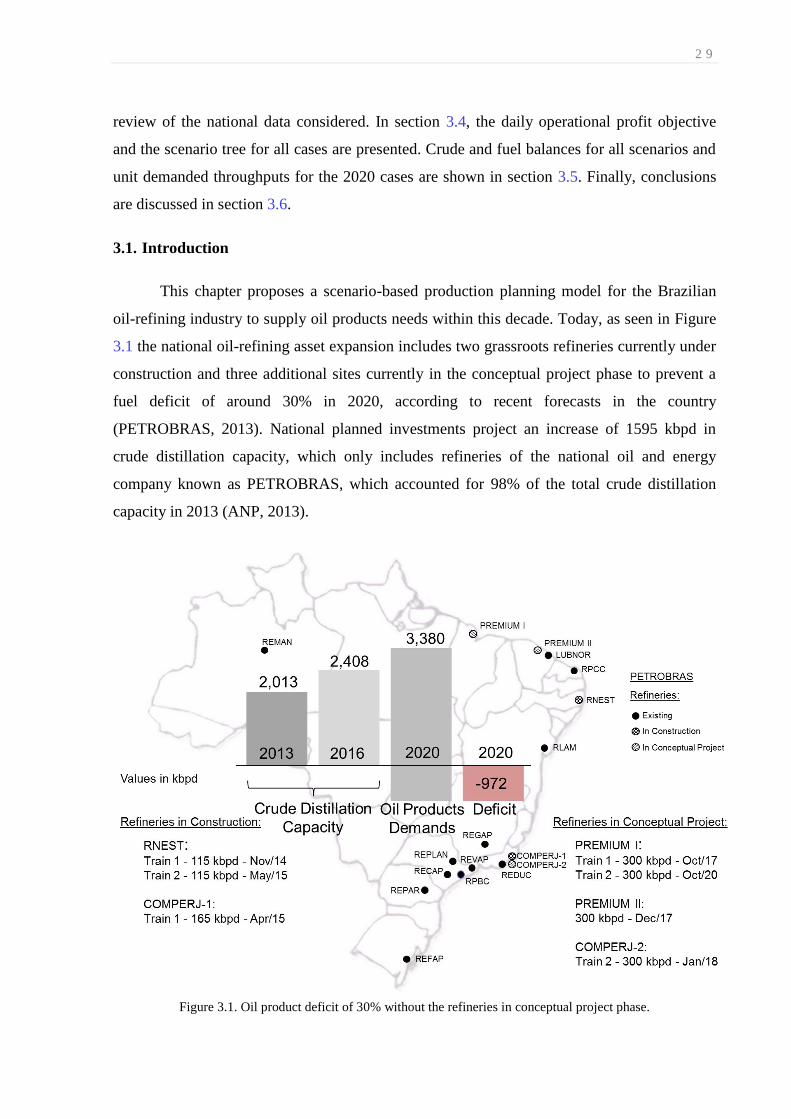
2 9

review of the national data considered. In section 3.4, the daily operational profit objective

and the scenario tree for all cases are presented. Crude and fuel balances for all scenarios and

unit demanded throughputs for the 2020 cases are shown in section 3.5. Finally, conclusions

are discussed in section 3.6.

3.1. Introduction

This chapter proposes a scenario-based production planning model for the Brazilian

oil-refining industry to supply oil products needs within this decade. Today, as seen in Figure

3.1 the national oil-refining asset expansion includes two grassroots refineries currently under

construction and three additional sites currently in the conceptual project phase to prevent a

fuel deficit of around 30% in 2020, according to recent forecasts in the country

(PETROBRAS, 2013). National planned investments project an increase of 1595 kbpd in

crude distillation capacity, which only includes refineries of the national oil and energy

company known as PETROBRAS, which accounted for 98% of the total crude distillation

capacity in 2013 (ANP, 2013).

Figure 3.1. Oil product deficit of 30% without the refineries in conceptual project phase.

3 0

The proposed approach predicts the overall capacity of oil-refinery units considering

the current Brazilian refineries aggregated in one hypothetical refinery called REBRA to

approximate the national overall capacity for several types of units. The single-period

nonlinear programming (NLP) operational planning model for REBRA defines the national

crude diet, unit throughputs, fuel production, and import amounts, taking into account profit

maximization in 2013, 2016, and 2020. Regarding the expected and proposed fuel market

scenarios for the conceptual projects in 2020, with planned overall capacities higher than their

demanded throughputs, the projects require refitting.

Different fuel market scenarios, including the gasoline-ethanol customer preference,

are proposed to cover all limiting demands. The final overall capacity planning results may

indicate project alteration once the refineries currently in the conceptual phase can still be

modified to find the best investment portfolio considering the future official and proposed

market scenarios defined in this work. A full review on the investment strategies for the future

fuel market in Brazil can be found in Appendix 0A.

3.2. NLP Operational Planning Model

Production and market scenarios are tested considering the NLP operational planning

model presented in this section. Figure 3.2 shows the oil-refinery unit framework considered.

For the cases under analysis, the hydrocracker (HCC) is excluded from the hypothetical

refinery for the current scenario in 2013 as well as the ability to process atmospheric residuum

(ATR) in a delayed coker unit (DC). For the 2016 and 2020 scenarios, both options are

considered.

3 1

Figure 3.2. Hypothetical refinery REBRA.

3.2.1. Swing-Cut distillation modeling

Distillation units are often modeled into several operational modes, such as maximum

gasoline, kerosene, or diesel (Brooks, 1999). Each mode is based on a set of temperature

cutpoints defined by previous experience, experimental data, or process simulators, so that

intermediate fractions can be managed to both adjacent distillates, creating swing cuts, which

can be included in a distillation model instead of considering the final distillates with fixed

yields and fixed properties based only on the pooled crude-oil feed. Thus, the swing-cut

modeling approximates the temperature cut-point variation without the need to recut the crude

assay (Di Vita, 2009)

The swing-cut approximation models the consequence of the thermodynamic variation

inside the distillation column, which, driven by pressure and temperature, allows some

hydrocarbon fractionation by creating internal cut swinging, which can be expressed as a

FK

FLD

ATR

CDUC1C2

C3C4

SW2

VR

VDU

N

K

LD

HD

LCO

DO

HTD

HTK

FCC

D1HT

KHT

CLN

CHN

CLGO

CHGO

CMGO

D2HT

DC

REF

LCNHT

CLNHT

PQN

C1C2

C3C4

HCN

LCN

C1C2

C3C4

FN

FHD

GLN

(GLNC)

MSD

JET

LSD

HTCLN

HTLCN

FO

REFOR

C1C2 FG

LPGC3C4

LVGO

HVGO

00

ASPR

DAO

PDA

RFCC

SW3

SW1

C1C2

C3C4

HCCO

Crude

HCCD

HCCK

HCCN

HCC

UHSD

COKE

H2

COKE

LSDimp

GLNimp

(GLNA)

ETH

DCA

JETimp

LPGimp

ST

GOST

LNST

HNST

FK, FLD

HSD

3 2

volume ratio on crude feed, as a certain boiling temperature range, or as volume/mass transfer

ratios. Zhang et al. (2001) used 5% and 7% volume ratios on crude feed as the sizes of the

naphtha/kerosene and kerosene/diesel swing cuts, respectively. Li et al. (2005) considers that

the swing cuts ranges are bounded by the union of three operational modes in the CDU (crude

distillation unit) taking into account maximization of naphtha, light diesel and heavy diesel to

find mass transfer ratios for the swing cuts. Despite the CDU processing-variance

consideration by the swing cuts modeling, these authors considered a fixed crude diet for their

cases, which reduces decision-making in planning and scheduling cases, and used Watkins

(1979) correlations based on yields to predict the final distillate properties and not the crude-

oil assay property data.

Unlike previous researchers, in this work the mixed crude oil given by the CDU feed

diet found in the model defines the blended fractions inside the distillation towers (cuts,

including the swing-cuts), and then a new pooling occurs to get the final distillate yield and

properties for an optimal volume yielding distribution given by the exchangeable cuts. These

swing cuts are split into light and heavy fractions, the former representing the swing-cut part

flowing to the light distillate and the latter representing the one flowing into the heavy

distillate. Optimization involving quantity variables for the light and heavy swing cuts and

quality variables for the whole swing-cut as presented in this work is found in commercial

planning platforms such as GRTMPS (Haverly), Aspen PIMS (Aspen Technology), and

RPMS (Honeywell). Their solutions include the crude diet and final distillate quality

optimization, both related to the cut and swing-cut internal blending modeling, by employing

home-grown successive linear programming algorithms to solve the nonlinearities. The

mentioned authors do not consider properties for the swing-cuts (Zhang et al., 2001) or

calculate the final distillates properties by empirical correlations based on distillate yields (Li

et al., 2005), nor do they consider crude-oil assay data as in this work, in which a typical 30-

40ºC true boiling temperature (TBP) range is set to the swing-cut fractions, which is already

expressed in the given crude-oil assay yields and properties.

Figure 3.3 shows the material flow for cuts c and final-cuts fc of the CDU. The light

and heavy swing-cut fractions mix with their upper (light) and lower (heavy) cuts,

respectively, internally to the tower and not as schematically presented.

3 3

Figure 3.3. Cut and swing-cut material flow modeling for CDU yields.

Given the CDU and VDU (vacuum distillation unit) configurations in Figure 3.2, the

crude is separated into different internal cut; some of them can swing (SW1, SW2, SW3)

between their adjacent final-cuts or final distillates as seen in Figure 3.3. Each crude cr to be

processed Qcr,CDU is defined as a CDU throughput QFCDU volume ratio cr as in Equation 3.1,

whose sum is calculated by Equation 3.2.

( )

∑

( )

The quantity of CDU/VDU internal cuts c flowing to the final-cuts fc Qc,fc is given by

crude-oil assay data in Table S3.1 (see the Supporting Information) and crude feed. Ycr,c

represents the yields for the CDU and VDU cuts (with some as swing-cuts) based on the

crude assay. Only the swing cuts flow to both adjacent final-cuts. For other cuts, the first sum

SW3-Cut

SW2-Cut

SW1-Cut

Naphtha

Kerosene

C1C2

C3C4

SW1

K

SW2

light

heavy

cuts (c) final cuts (fc)

TBP (ºC)

-163.524

27.878

40

130140150160170

180

210220230

200190

240Light Diesel

Crude Assay

Yields Ycr,c(%)

100

250

Heavy Diesel

N

5060708090

36.059

120110

SW3

260270280

310320330

300

LD

290

340 HD350

.

360

.

....

Naphtha-Cut

Kerosene-Cut

light

heavy

Light Diesel-

Cut

light

heavy

Heavy Diesel-

Cut

-88.599

crude (cr)

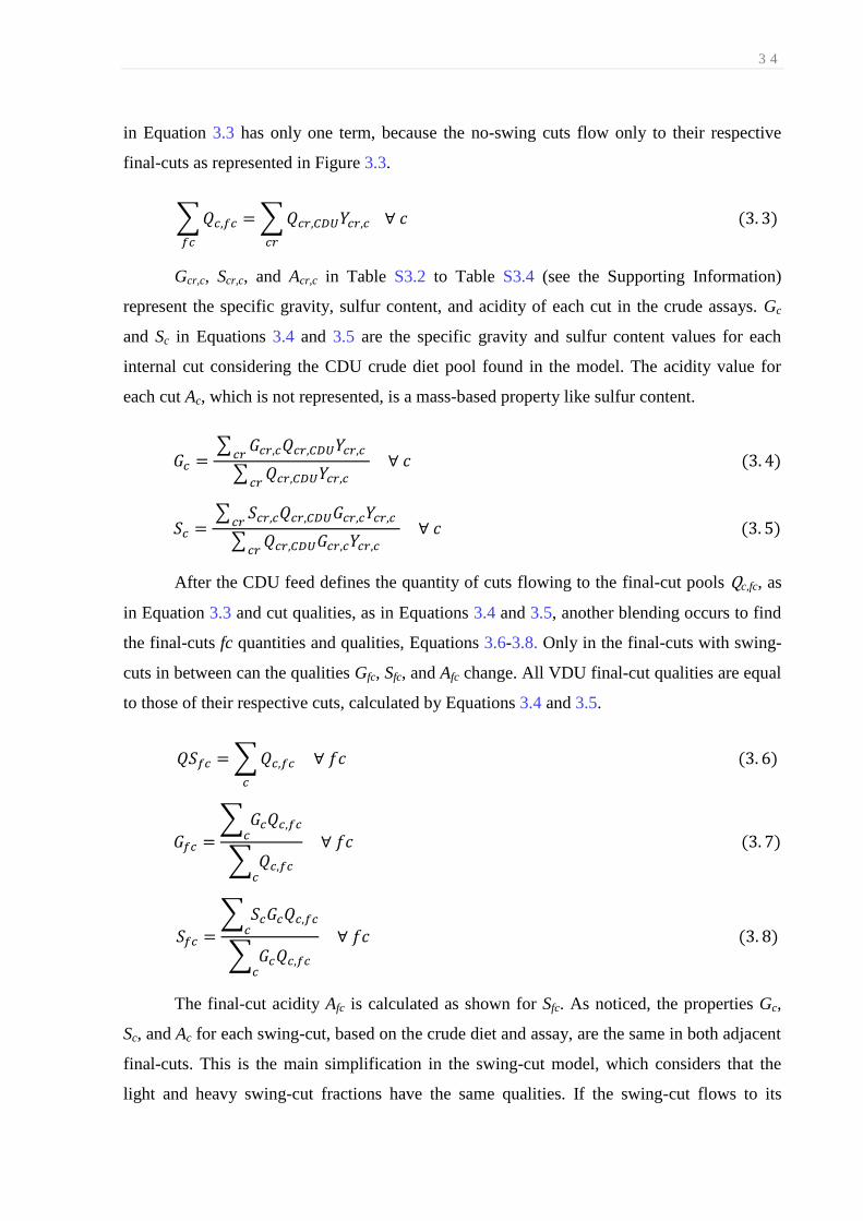
3 4

in Equation 3.3 has only one term, because the no-swing cuts flow only to their respective

final-cuts as represented in Figure 3.3.

∑

∑

( )

Gcr,c, Scr,c, and Acr,c in Table S3.2 to Table S3.4 (see the Supporting Information)

represent the specific gravity, sulfur content, and acidity of each cut in the crude assays. Gc

and Sc in Equations 3.4 and 3.5 are the specific gravity and sulfur content values for each

internal cut considering the CDU crude diet pool found in the model. The acidity value for

each cut Ac, which is not represented, is a mass-based property like sulfur content.

∑

∑

( )

∑

∑

( )

After the CDU feed defines the quantity of cuts flowing to the final-cut pools Qc,fc, as

in Equation 3.3 and cut qualities, as in Equations 3.4 and 3.5, another blending occurs to find

the final-cuts fc quantities and qualities, Equations 3.6-3.8. Only in the final-cuts with swing-

cuts in between can the qualities Gfc, Sfc, and Afc change. All VDU final-cut qualities are equal

to those of their respective cuts, calculated by Equations 3.4 and 3.5.

∑

( )

∑

∑

( )

∑

∑

( )

The final-cut acidity Afc is calculated as shown for Sfc. As noticed, the properties Gc,

Sc, and Ac for each swing-cut, based on the crude diet and assay, are the same in both adjacent

final-cuts. This is the main simplification in the swing-cut model, which considers that the

light and heavy swing-cut fractions have the same qualities. If the swing-cut flows to its

3 5

adjacent lighter distillate it carries heavy ends, which will influence properties such as sulfur

content and gravity of the lighter distillate. Similarly, moving the swing-cut to its adjacent

heavier distillate will bring light ends, particularly affecting properties such as the viscosity

and flash point, which are more sensitive to light ends (Li et al., 2005). In the context of this

work, this simplification is quite acceptable for strategic plans, and an improved swing-cut

model addressing quality variations for both light and heavy swing-cut streams will be seen in

Chapter 5. A similar approach to that of the swing-cut model described in this work is used by

the Energy Information Agency (EIA) to plan fuel balance in the United States (Divita, 2009);

however, it considers average fixed qualities for the final distillates, as it is being treated here

for other unit output stream properties.

We consider the yield and property variations to predict distillation tower outputs by

permitting crude-oil diet and final-cut variation, a big step toward improve the planning

results in a high-level decision-making model in the oil-refining industry. Despite model

improvements by considering nonlinearities, which in turn tend to be ill-conditioned when

size increases, global optimal solutions are not a guarantee in non-convex models. Initial

value randomization and do/loop searching can find better results iteratively.

3.2.2. Other oil-refinery units

As mentioned, product yields and properties for other oil-refinery units are considered

averaged fixed values. The yield Yu,s for each stream s is given as a unit throughput ratio

forming the output or stream flows QSu,s, as seen in Equation 3.9. All necessary data are given

in Table S3.5 (see the Supporting Information).

( )

Moro et al. (1998), Pinto et al. (2000), and Neiro and Pinto (2004) modeled

operational planning and scheduling cases for refining process units considering a network

whose streams are linked to them by mixers and splitters as shown in Equations 3.10 and

3.11; the former concentrates streams from upstream unit u’ (u’ up) into the unit u, and the

latter distributes the unit streams or outputs to downstream unit u’ (u’ do). The units are

connected considering the framework shown in Figure 3.2.

3 6

∑

( )

∑

( )

As specific gravity and sulfur content are included in the model to allow variations in

the final product qualities based on crude diet and swing-cut variations, it is important to

consider modification of properties in hydrotreaters (HT). The unit removes sources of

molecular instability and contamination such as sulfur, nitrogen, metals, and unsaturated

hydrocarbons. As the unit operates at high pressure and temperature, some molecular cracking

inevitably occurs; thus, some properties such as specific gravity and octane number change. In

this work, sulfur reduction promoted by the hydrotreaters is modeled as a variable HT,t, as

seen in Equation 3.12. The lower and upper bounds for the medium and high severity

hydrotreaters for diesel are 0.800 ≤ D1HT ≤ 0.980 and 0.960 ≤ D2HT ≤ 0.998, respectively.

For gasoline hydrotreaters (LCNHT and CLNHT) are 0.500 ≤ LCNHT/CLNHT ≤ 0.990. Severity

in kerosene hydrotreater (KHT) is not being considered. The specific gravity reduction factor

ΔHT promoted by residual molecular cracking is treated as a fixed value for all hydrotreaters

like in Equation 3.13 and its value in this work is 0.99.

( ) ( )

( )

Specific gravity GHT and sulfur content SHT in hydrotreater feed are volume- and mass-

based properties calculated by Equations 3.7 and 3.8, respectively, considering the final

distillates or final-cuts fc as a unit feed mix (mixer) and the cut properties (Gc and Sc) as the

properties of each upstream flowing to the unit. The properties for the blended crude-oil

processed and intermediate and final products are found in the same way. Mixing and splitting

involving oil-refinery units, other blending rules and properties, and other processing

transformations can be found in mentioned authors (Moro et al., 1998; Pinto et al., 2000; and

Neiro and Pinto, 2004).

3 7

3.2.3. Octane number calculation: Ethyl equation

The octane number calculations presented in Equations 3.14 and 3.15 are the ethyl

formulations to predict the research octane number RON and motor octane number MON

needed to determine the retail gasoline recipe. The octane rating or number is a gasoline

property related to the combustion efficiency in Otto cycle engines in which the maximum

compression ratio is intended at the ignition spark, avoiding spontaneous ignition under high-

pressure conditions.

The blending correlation for RON and MON is highly nonlinear and depends on the

recipe components to be calculated, because it considers molecular interactions based on the

aromatic ARO and olefin OLE contents. RONVs and MONVs represent blending values for

RON and MON of each component in the gasoline pool, whose final RON and MON values

are volume-based properties considering blending values RONVs and MONVs as the

component properties. The blending value of a blending component changes with the

molecular composition and recipe; thus, it is different for every blend (Barsamian, 2007).

RONs, MONs, OLEs and AROs represent properties for each stream s, component of the

gasoline formulation as shown in Figure 3.2. They are fixed for the streams in Table S3.5 (see

the Supporting Information) and calculated as a blend for coker light naphtha hydrotreater

(CLNHT) output and for the gasoline C (GLNC) blender stream. Js is the octane number

sensibility defined as RONs-MONs. JV (RONV-MONV), RONV, MONV, OLEV, and AROV are

volume-based properties. AROVQ is the volume-based property for ARO2. The coefficients a to

g are given in Table S3.6 (see the Supporting Information), but they can be determined

experimentally. RON and MON decrease by values of 1.2 and 1 after hydrotreating units.

[( )( )] ( )

( )

[( )( )] ( )

[( )( )] ( )

[ ( ) (

)

( )

] ( )

3 8

3.3. Problem Statement: The Brazilian Oil Industry Scenario

Using the proposed NLP operational planning model, it is analyzed the national fuel

balance of each scenario taking into account the situation in 2013 and the planned investments

and different product demands in 2016 and 2020. Data from several official sources were

considered to represent the situation in 2013 that is the baseline on which the other ones were

drawn. The national fuel production and processed crude results are used to validate the

scenario in 2013. In the next subsections the available data on the Brazilian oil-refining

industry and the production and market scenarios are presented.

3.3.1. Fuels demands and production

Figure 3.4 shows the national fuel production and demands during the period 2000-

2012 and the future demands considering the 2009-2012 boost in fuel demands in the country.

In the work it is proposed future fuel market scenarios considering (1) 4.2% p.a. (per year) for

all fuels, based on the Brazilian GDP forecast (ANP, 2013) and (2) 2009-2012 trends for each

fuel as in Figure 3.4 considering GLNC and GLNCETH scenarios for gasoline.

Figure 3.4. Demand and production levels and forecast considering the 2009-2012 trends.

The boost in national fuel demands after the 2008-2009 global crisis is considered a

representative alternative for the future market scenarios. This situation is a consequence of

the economic growth in the country and is still expected to rise even with the economic and

3 9

political instability in Brazil that emerged in 2013 and the 2008-2009 economic crisis uprising

return worldwide.

3.3.2. Gasoline-Ethanol mix and ethanol for fueling

Ethanol commercialization presents particular dynamics for small and medium cars

fleets in Brazil. It can be part of the retailed gasoline and up to 100% fuel in flex-fuel fleets.

The ethanol content in the retailed gasoline varies between 25 to 18% in volume, a proportion

controlled by the ethanol market demand and prices. During periods when the country needed

to import ethanol to blend into gasoline A (pure gasoline, without ethanol), the ethanol

content was 18%. The value considered in this work is 25% which is the current situation

without any influence from the ethanol market, a preferred condition due to the gasoline

deficit in the country. Retailed gasoline (GLNC) is a mix of gasoline A (GLNA) and ethanol

permitted by the blended volume range (25 to 18% in volume). Ethanol content higher than

25% in gasoline can negatively affect the performance of a non-flex-fuel automobile and

intensify corrosion problems inside the motor. Today in Brazil, flex-fuel fleet sales represent

90% of the market in both the small- and medium-car categories, and it is expected that the

total flex-fuel fleet in these categories, currently at around 60%, will reach 80% within the

next 5 years.

In addition to the normal demand increase in fuels, the GLNC demand increase in the

period 2009-2012 (11.8% p.a.) was influenced by the ethanol for fueling (ETH) to GLNC

consumer preference shift. This occurred because of the ethanol price surge, which was an

effect of nationwide sugar cane harvesting problems in 2009 and of the escalation of sugar

demand overseas, both of which shaped the current ETH-GLNC fuel preference. Besides, the

widening demand for retailed gasoline maintains the ethanol demand and price growth once

ethanol is included in its formulation. As a consequence, the relative price between ethanol

for fueling and retailed gasoline remains higher than 0.7, so that gasoline is more attractive for

fueling. Considering the heats of combustion and engine efficiency of both fuels, when ETH

prices are higher than 70% of the GLNC it is considered more profitable to fuel the car. For

values lower than 70%, ETH is preferred. This fact is well-known to the consumer who

compares the ETH/GLNC relative price and decides which fuel to buy.

Considering the gasoline/ethanol market stabilization, the retailed gasoline demand

growth considered in Figure 3.4 is 7.2%, which is its increase discounting the ethanol for

4 0

fueling demand decrease during 2009-2012, hence excluding the influence of the ETH (100%

ethanol) shift. As shown, the ETH shift to GLNC reached its steady state in 2012, and on the

bases of this fact, we consider that the range of demand for retailed gasoline plotted in the

graph represents the equilibrium between GLNC and ETH driven by the consumer of the flex-

fuel fleet. GLNC is the current situation considering the ETH shift stabilization, and

GLNCETH is the situation where the ETH demand decrease is discounted from the retailed

gasoline demand increase between 2009 and 2012.

3.3.3. Future fuels demands

This work simulates the production and market scenarios in an operational planning

manner to find the best operational setting, so the future fuel demands are given in a daily

flow considering the demand scenarios shown in Table 3.1. Table 3.2 shows the diesel grade

evolution for the next several years (MPF, 2009), which is taken into consideration when

future diesel demands are defined.

Table 3.1. Demand forecast for 2016 and 2020.

Table 3.2. Diesel grades market.

2013* 2016 2020 2016 2020

LPG 36.2 38.6 41.2 42.6 50.2

gasoline C GLNC 112.4 148.8 196.8 132.5 156.2

GLNCETH 90.6 119.9 158.6 106.8 125.9

jet fuel JET 19.7 26.4 35.5 23.2 27.3

diesel 10 wppm DSL 16.0 60.6 153.0 56.6 133.5

500 wppm 80.1 90.9 51.0 84.9 44.5

1800 wppm 56.0 40.4 45.9 37.7 40.1

3500 wppm 8.0 10.1 5.1 9.4 4.5

Diesel Total 160.1 202.0 254.9 188.7 222.5* past 12 months until October, 2013 (ANP, 2013)

2009-2012 trends 4.2% p.a.

product

liquid petroleum gas

gasoline C – ethanol

2013 2016 2020

10 wppm S 10% 30% 60%

500 wppm S 50% 45% 20%

1800 wppm S 35% 20% 18%

3500 wppm S 5% 5% 2%

4 1

3.3.4. Current and planned capacities in 2013, 2016 and 2020

The refinery configuration considered in the work is shown in Figure 3.2. Table 3.3

shows the capacities of the units for the three production scenarios aforementioned. All data

regarding the overall oil-refinery units capacities considered for the productive scenarios are

presented in Perrissé (2008). In the cases of study, the minimum feed allowed for the units is

68% of their overall capacity, excepted in the units showed with a mark * in Table 3.3 and in

the propane deasphalting unit (PDA), which is 30%.

Table 3.3. Overall refining processes capacities for the three production scenarios (k m3/d), excluding lubricant

plants.

3.3.5. National and imported crude oils

Figure 3.5 shows crude-oil amounts considering national production, imports, and

processing as well as the export and import prices. As shown, since 2008 the country has been

self-sufficient in equivalent oil but still needs ultralight oil imports to increase medium

distillate (jet fuel and diesel) production and paraffinic oil for lubricants.

2013 2016 2020

crude distillation unit (CDU) 310* 372* 536

vacuum distillation unit (VDU) 140* 153* 260

residue fluid catalytic cracking (RFCC) 22 22 22

fluid catalytic cracking (FCC) 76 76 76

hydrocracking (HCC) 10 74

propane deasphalting (PDA) 10 10 10

delayed coker (DC) 42 50 100

delayed coker with atmosferic residue as feed (DCA) 24* 24*

light cracked naphtha hydrotreater (LCNHT) 54 54 54

coker light naphtha hydrotreater (CLNHT) 22 34 62

stabilizer (ST) 22 34 62

kerosene hydrotreater (KHT) 15* 15* 15*

diesel hydrotreater (medium severity) (D1HT) 60* 60* 60*

diesel hydrotreater (high severity) (D2HT) 30* 68* 135

reformer (REF) 7 12 20**

* upper and lower bounds are the same to avoid local solution

** added 8 k m3/d arbitrarily (different from conceptual project) to yield feasible results

4 2

Figure 3.5. Crude-oil produced, imported and processed and imports and export prices (ANP, 2013).

In Figure 3.6, the national oil production is distributed in four ºAPI ranges (ultralight,

light, medium, heavy) and the average ºAPI and sulfur content of each group are shown as

well as the national average values (24.36 ºAPI and 0.536 % S).

Figure 3.6. National crude-oil production in 2012 (ANP, 2013).

In this work five different crude oils are considered to represent the national and

importd groups. The national medium crude is split into presalt and medium. The presalt

crude is considered medium-light to light oil and represented 14% of the entire national

production in 2012. Ultralight crude is given to represent the imports to achieve the optimal

ºAPI for the crude blend to be processed in the Brazilian fuel market and production

scenarios. The crude oils considered are shown in Table 3.4 and the crude diet upper bounds

max of the national crude to be processed are defined by their production in 2012 as seen in

Figure 3.6. For the 2016 and 2020 scenarios, the presalt crude is predicted to increase to 22%

and 33%, respectively, as expected by PETROBRAS (PETROBRAS, 2013a), and the

4 3

medium upper bound ratio is reduced to maintain medium and presalt crude sum in 66% as

considered in Figure 3.6.

Table 3.4. Crude oils considered in this work.

3.3.6. Crude and fuel prices

Crude and fuel prices and their sources are shown in Table 3.5. The price baseline is

considered that in 2013 with a growing rate of 4.2% per year (p.a.) as expected for the GDP

rate considered in this work. Crude prices per m3 of US$ 702 for the imported oil and US$

587 for the exported oil are considered (average value in the past 12 months until October,

2013) (ANP, 2013). The country exports unprocessed heavy and medium crude, and

considering the national heavy crude price of US$ 570 and the exported crude composed by

30% medium and 70% heavy (in volume), the medium oil price estimate is US$ 592. For the

national light and presalt crude, prices take an intermediate value between national medium

and Brent oils, closer to the medium, because they are national crude and heavier than the

Brent. The standard crude-oil Brent (38 ºAPI, 0.45 % S) price considered is US$ 687 (US$

109.2 per barrel) in the North Sea port (EIA, 2013). Fuel prices are defined by the retail prices

in the past 12 months until October 2013 (ANP, 2013; UNICA, 2013) and the producer

percentages shown in Figure 3.7. The imported prices consider the U.S. Gulf Coast region

(EIA, 2013), adding transport expenses and taxes.

Figure 3.7. Fuels prices percentage (PETROBRAS, 2013b; Agencia T1, 2013).

ºAPI G (g/cm3) S (%) A (mgKOH/g) max

national light 33.2 0.859 0.091 0.226 0.09

presalt 29.7 0.878 0.344 0.255 0.14

medium 25.2 0.903 0.519 0.196 0.52

heavy 20.5 0.931 0.608 1.007 0.25

imported ultra light 45.2 0.801 0.049 0.096

crude

4 4

Table 3.5. Prices (US$/m3) of crude, products, and imports in Brazil grow at a rate 4.2% p.a.

3.3.7. Crude and fuel quality specifications

Upper and lower bounds of the CDU feed properties and the specifications of final

product properties are shown in Table 3.6.

Table 3.6. CDU feed and final products property specifications.

2013 2016 2020

crude* national light 600.0 678.8 800.2

presalt 595.0 673.2 793.6

medium 592.0 669.8 789.6

heavy 570.0 644.9 760.2

imported ultralight 702.0 794.2 936.3

products*

FG

LPG 380.0 429.9 506.8

naphtha 545.0 616.6 726.9

gasoline C 618.3 699.5 824.7

jet fuel 760.0 859.8 1013.6

diesel 10 wppm S 662.0 749.0 882.9

500 wppm S 636.0 719.5 848.3

1800 wppm S 623.3 705.2 831.3

3500 wppm S 610.8 691.1 814.7

FO 416.0 470.6 554.8

coke 530.0 599.6 706.9

ethanol§

590.0 667.5 786.9

imports† LPG 398.2 450.5 531.1

gasoline A 762.3 862.4 1016.7

jet fuel 860.0 973.0 1147.0

diesel 15 wppm S 834.1 943.7 1112.5*ANP (2013)

§UNICA (2013)

†EIA (2013)

Gmin Gmax S max Amax MON min RON min

CDU feed 0.850 0.950 0.800 0.60

GLN (GLNC) 0.720 0.775 0.005 82 88

JET 0.771 0.836 0.300

DSL 10 wppm S 0.820 0.850 0.001

500 wppm S 0.820 0.865 0.050

1800 wppm S 0.820 0.880 0.180

3500 wppm S 0.820 0.880 0.350

S [=] % A [=] mgKOH/gG [=] g/cm3

4 5

3.3.8. Other relations

Two other constraints are related to (i) the current official ethanol content in the

retailed gasoline pool (GLN), Equation 3.16, and (ii) the maximum concentration of coker

light naphtha (CLN) from delayed coker units (DC or DCA) in the coker light naphtha

hydrotreater (CLNHT) feed, Equation 3.17. This upper bound for CLN streams protects the

catalyst bed from high metal concentration poisoning.

( )

( )

3.4. Operational Planning Objective: Daily Operational Profit

Eight future scenarios in 2020 are illustrated in Figure 3.8. At the first, consumer

preference between ethanol for fueling and retail gasoline is taken as a starting point by

discounting and not the ethanol shift proposed previously (see Figure 3.4). The second choice

is the demand increase rate considering 2009-2012 trends for each fuel and 4.2% p.a. for all,

and the last option is to consider the refineries in conceptual design to be built or not in 2020

in order to avoid a deficit of 30% in oil products. Crossover over the time is not permitted; so

that once a scenario option is selected it is true for the following scenarios.

Figure 3.8. Initial, intermediate, and final scenarios considered.

4 6

The single-period objective function in millions of U.S dollars per day is summarized

in Equation 3.18. Operational costs from inventory, utilities (steam, water, hydrogen,

nitrogen, fuel gas, electricity), and materials like catalysts and chemicals are not directly

considered in the model. Refcost approximates the overall refining costs in US$ 4.5 per barrel

of product (US$ 28.3/m3) for a standard production cost at American refineries (EIA, 2013).

Additionally, to avoid sulfur content giveaway when we have different grades of diesel, it is a

good practice is to consider hypothetical blender for each grade and HT operational costs

defined as a function of its feed flow QFHT similar to a penalty in the objective function. The

taxes are discounted from the profit considering a fixed tax ratio tr of 25%, what is a practice

in Brazil for companies’ profit taxes.

The operational planning model includes Equations 3.1-3.18. The crude amounts

QFcr,CDU are determined by prices pr, product demands, processing structure, and product

specifications like specific gravity, octane number, sulfur content and acidity. Products

amounts QFp supplying demands are set to be only 1% apart, avoiding surplus of any fuel.

( ) (∑( )

∑

∑

∑

) ( )

Seasonal variations regarding demands can be considered by verifying the level of

flexibility for the refining framework for gasoline and diesel maximization modes. Annual

average demand data of 2013 are used as the baseline for the cases in analysis, so these

seasonal variations are not being included in the scope of this work.

3.5. Results and Discussion

The national refining framework and fuel market demands in October 2013 are the

baselines to find the intermediate scenarios for 2016 and the eight scenarios for 2020 as

previously defined. For the 2020 cases with the projects in the conceptual phase performed, if

the unit throughput is lower than the planned capacity, which in the model is the throughput

upper bound , the country’s capacity planning for 2020 needs refitting. All case studies

were implemented in the GAMS modeling system (Brook et al., 2002), version 23.9.3, on an

Intel Core 2 Duo (3.00 GHz, 16.0 GB of RAM) and used as starting points unit capacities,

4 7

output standard values for flows and given specifications for calculated properties. The

overall data given in this work can be used to find initial values. The NLP problems are

solved by nonlinear general-purpose optimizers such as CONOPT, which is based on the

reduced gradient method, IPOPT, which utilizes interior point methods, and the solver

SNOPT, which is based on successive quadratic programming.

3.5.1. Pricing policy in 2013

Table 3.7 shows the profit obtained to match country’s demands in the 2013 GLNC

baseline scenario (Table 3.1) considering different pricing policies. As indicated, the current

refining activity in Brazil is not profitable on a stand-alone view. This is a well-known

condition due to the lower national producer prices of gasoline and diesel in comparison with

import prices. If prices in U.S. Gulf are considered for gasoline and diesel 15 wppm S (682.43

and 760.89 US$/m3, respectively), the national-international (Brazil-US) loss difference (-

16.761 million US$/d) is close to the estimate of the Brazilian Center of Infrastructure

(OGLOBO, 2013), which evaluated losses from January to May, 2013 of 2.2 billion US$ (-

14.379 million US$/d). The prices for other grades of diesel have the same price relation

found in Table 3.5. As the country needs to import gasoline and diesel to supply the market,

the price difference between domestic market and imports is bore by the national oil and

energy company PETROBRAS. Although the country needs to import LPG and jet fuel, these

fuels do not damage the company’s profitability because of the state LPG subsidies and the jet

fuel uncontrolled prices. Currency variation along the year is not being considered and it is

fixed in 2.2 R$/US$.

The new pricing policy announced Nov 29, 2013 increased the producer price of retail

gasoline by 4% and diesel by 8%, but this move was not sufficient to overcome the daily

refining losses in the country (-13.786 million US$/d). In this work it is considered price

increases of 15% for retail gasoline and 20% for diesel in its different grades to yield a

positive gain (1.068 million US$/d). This price rise is evaluated by the market as the

demanded pricing policy to avoid losses and get a minimal margin return (of around US$

0.5/barrel). This obtain positive gain policy is considered to calculate future scenarios in the

daily single-period NPL operational planning model for fixed production frameworks in 2013,

2016, and 2020.

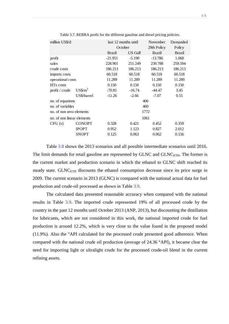
4 8

Table 3.7. REBRA profit for the different gasoline and diesel pricing policies.

Table 3.8 shows the 2013 scenarios and all possible intermediate scenarios until 2016.

The limit demands for retail gasoline are represented by GLNC and GLNCETH. The former is

the current market and production scenario in which the ethanol to GLNC shift reached its

steady state. GLNCETH discounts the ethanol consumption decrease since its price surge in

2009. The current scenario in 2013 (GLNC) is compared with the national actual data for fuel

production and crude-oil processed as shown in Table 3.9.

The calculated data presented reasonable accuracy when compared with the national

results in Table 3.9. The imported crude represented 19% of all processed crude by the

country in the past 12 months until October 2013 (ANP, 2013), but discounting the distillation

for lubricants, which are not considered in this work, the national imported crude for fuel

production is around 12.2%, which is very close to the value found in the proposed model

(11.9%). Also the °API calculated for the processed crude presented good adherence. When

compared with the national crude oil production (average of 24.36 °API), it became clear the

need for importing light or ultralight crude for the processed crude-oil blend in the current

refining assets.

Brazil US Gulf Brazil Brazil

profit -21.951 -5.190 -13.786 1.068

sales 228.901 251.249 239.788 259.594

crude costs 186.213 186.213 186.213 186.213

imports costs 60.518 60.518 60.518 60.518

operational costs 11.289 11.289 11.289 11.289

HTs costs 0.150 0.150 0.150 0.150

profit / crude US$/m3

-70.81 -16.74 -44.47 3.45

US$/barrel -11.26 -2.66 -7.07 0.55

no. of equations

no. of variables

no. of non zero elements

no. of non linear elements

CPU (s) CONOPT 0.328 0.421 0.452 0.359

IPOPT 0.952 1.123 0.827 2.012

SNOPT 0.125 0.063 0.062 0.156

million US$/d last 12 months until

October

November

29th Policy

Demanded

Policy

406

460

1772

1061

4 9

Table 3.8. 2013 and 2016 production and market scenarios (thousand cubic meter per day [=] k m3/d).

Table 3.9. Actual and calculated data for the current scenario (GLNC) in 2013.

The calculated data presented reasonable accuracy when compared with the national

results in Table 3.9. The imported crude represented 19% of all processed crude by the

country in the past 12 months until October 2013 (ANP, 2013), but discounting the distillation

for lubricants, which are not considered in this work, the national imported crude for fuel

production is around 12.2%, which is very close to the value found in the proposed model

(11.9%). Also the °API calculated for the processed crude presented good adherence. When

compared with the national crude oil production (average of 24.36 °API), it became clear the

need for importing light or ultralight crude for the processed crude-oil blend in the current

refining assets.

GLNC GLNCETH GLNC GLNCETH GLNC GLNCETH

national light 9.0 9.0 9.0 9.0 9.0 9.0

presalt 14.0 14.0 22.0 22.0 22.0 22.0

medium 40.1 40.1 33.6 33.6 33.6 30.9

heavy 25.0 25.0 25.0 25.0 25.0 25.0

imported ultralight 11.9 11.9 10.4 10.4 10.4 13.1

national 16.8 16.3 20.7 20.7 20.7 20.3

imported 19.3 19.9 17.9 17.9 21.9 22.3

sales 36.2 36.2 38.6 38.6 42.6 42.6

national GLNA 72.1 68.0 84.0 83.6 83.8 80.1

imported GLNA 12.3 27.6 6.3 15.6

Ethanol 28.1 22.7 37.2 30.0 33.1 26.7

sales GLNC 112.4 90.6 148.8 119.9 132.5 106.8

national 15.0 15.0 16.8 16.8 16.8 16.8

imported 4.7 4.7 9.6 9.6 6.4 6.4

sales 19.7 19.7 26.4 26.4 23.2 23.2

national 10 wppm S 16.0 16.0 60.6 60.6 56.6 56.6

500 wppm S 52.6 51.1 56.9 56.9 64.2 65.3

1800 wppm S 56.0 56.0 40.4 40.4 37.7 37.7

3500 wppm S 8.0 8.0 10.1 10.1 9.4 9.4

imported 15 wppm S 27.4 29.0 34.0 34.0 20.7 19.7

sales 160.1 160.1 202.0 202.0 188.7 188.7

2013 2016

2009-2012 trends 4.2% p.a.

crude diet

(% vol)

LPG

gasoline C

(GLNC)

jet fuel

(JET)

diesel

(DSL)

actual*

calculated actual*

product calculated

27.9 ºAPI 27.6 22.2 LPG 16.8

12.2 imported (%) 11.9 76.4 GLNA 72.1

15.3 JET 15.0

133.3 DSL 132.7

Fuel Production (k m3/d)Processed Crude

*past 12 months until October, 2013 (ANP, 2013 )

5 0

Considering the main fuel production, the lower LPG found is expected since the

model excludes LPG from CDU for lubricants, lubricant plants, and production from liquid

natural gas plants and condensates. The lower GLNA obtained is a result of the production

from non-PETROBRAS refineries excluded in this model, whose daily gasoline A production

reaches around 4 k m3/d. For JET and DSL the model presented good match compared with

the actual data.

The GLNCETH case in 2013 shows that, without the ethanol to gasoline market shift

after 2009, the country would be able to cease gasoline imports, as in the period before the

current flex-fuel fleet consumer preference setup between retail gasoline and ethanol for

fueling. The GLNCETH scenario lower profit in 2013 (see Table 3.10) is due to the lower FCC

throughput and CDU stream differences comparing with the GLNC counterpart. It occurs to

avoid fuel surplus, in this case for gasoline, and the outcome is higher LPG and diesel imports

in the GLNCETH scenario (see Table 3.8). Besides, the lower ethanol price (US$ 590/m3)

mixed at 25% in volume with refined gasoline (GLNA) to produce GLNC (US$ 711/m3)

contributes for higher profits in the GLCN scenario.

In the 2016 (2009-2012 trends) scenarios, the GLCN case presented lower profit.

Crude diet, LPG, kerosene and diesel imports are similar in both GLNC and GLCNETH

scenarios (see Table 3.8), and only the costs related to gasoline and ethanol imports and the

operational costs are varying in the profit calculation comparing both gasoline scenarios. As

the GLCN-GLCNETH deltas for sale amounts and import costs are practically equivalents, the

higher operational costs in the GLNC pair (of 0.924 million US$/d) explain its lower profit.

In the 2016 (4.2% p.a.) scenarios, the GLCNETH pair presented lower profit. In this

case, the GLCN-GLCNETH deltas for sale amounts, import costs, and operational costs are

practically equivalents, but the crude diet in the GLCNETH scenario uses more ultralight oil

(see Table 3.8), which has higher prices.

The size of the models is shown in Table 3.10. For the 2016 and 2020 scenarios HCC

was added and, as defined for the RNEST refinery, a new DC receiving ATR (DCA) as feed

with a capacity equal to 24 k m3/d is added. All three solvers (CONOPT, IPOPT, SNOPT) can

solve the problems in less than 1 second and converge to the same result (profit) in each of the

six scenarios in Table 3.10.

5 1

Table 3.10. Economic and model data for the 2013 and 2016 scenarios.

3.5.2. Conceptual project scenarios in 2020

The proposed scenarios in 2020 take into account the projects in conceptual phase and

whether they are executed for the four market scenarios; hence, eight cases are presented, as

shown in Figure 3.8, with maximum and minimum investment and import cases. As shown in

Table 3.11, in the four cases with projects in conceptual phase executed in 2020 (0% deficit)

as planned, the unit throughput results indicate different overall capacity in all market demand

cases, so the set of units to be expanded or installed needs refitting. In the 0% deficit cases is

in real permitted fuel imports. It is only labeled 0% to contrast with the -30% deficit if the

projects in conceptual phase were not executed.

The scenarios for 2020 in which the projects under conceptual phase were not

executed lead to significant fuel import amounts, resulting in unacceptable high expenditures,

trade deficit, and external dependence at critical levels. For the cases with the projects

executed, only in the lower demand scenarios (4.2% and GLNCETH) can the country be free of

gasoline, jet fuel, and diesel imports. For the cases that cannot count on the investments in the

conceptual phase, the crude import remains at 9.8 and 7.6% for the 2009-2012 trends and

4.2% p.a., respectively, even with the presalt crude level at 33%. For the cases with

investments, only in the scenario with maximum demands is it necessary to continue with

crude import, but at a slight level (5.8%). In the other three cases, the country becomes free of

GLNC GLNCETH GLNC GLNCETH GLNC GLNCETH

profit 1.068 0.161 3.529 4.177 5.150 4.482

sales 259.594 246.861 371.013 347.801 345.381 326.415

crude costs 186.213 186.213 252.249 252.249 252.249 253.475

imports costs 60.518 49.445 98.063 74.911 71.189 52.625

operational costs 11.289 10.843 15.797 14.873 14.878 14.145

HTs costs 0.150 0.146 0.199 0.199 0.199 0.195


3.45 0.52 9.49 11.23 13.84 12.05

US$/barrel 0.55 0.08 1.51 1.79 2.20 1.92

no. of equations

no. of variables



CPU (s) CONOPT 0.515 0.374 0.655 0.453 0.608 0.514

IPOPT 0.469 1.591 0.826 0.702 0.639 0.874

SNOPT 0.078 0.078 0.156 0.125 0.110 0.140

million US$/d 2013 2016

2009-2012 trends 4.2% p.a.

1061 1276

406 466

460 532

1772 2115

5 2

oil imports. In Table 3.12 the economic data for the scenarios in 2020 are shown. As

expected, all cases with investments are more profitable because of lower fuel imports.

Additionally, to explore the comparison between the required and the planned

capacities for 2020, GLNA, JET, and DSL imports were set to zero. But the results got

feasible only in the minimum demands scenario (4.2% and GLNCETH). Table 3.11 shows the

results for this case at the last column. The unit throughputs got higher upper bounds than its

counterpart with relaxed fuel imports requirements. However, as shown in Table 3.12, the

profit in this case was lower because of the additional crude expenses to feed the CDU, which

is higher than the import costs decrease. When the refineries in conceptual project were

defined before 2009, the strategic decisions considered were to be free of main fuel imports

(GLNA, JET, and DSL) in 2020 and the gasoline ethanol market shift was not in mind at that

time. In this way, the last column of Table 3.11 and Table 3.12 represents roughly the official

scenario in the country used to plan unit capacity expansions for 2020. In this work, an overall

4.2% p.a. demand increase was adopted for the low fuel demand cases, as described in

PETROBRAS business plan 2013-2017 (PETROBRAS, 2013a), which in real should have a

different distribution growth rate throughout the different fuels. In the fuels production charts

presented in the next subsection, the official scenario in 2020 (4.2% p.a. and GLNCETH)

without GLNA, JET, and DSL import is considered.

Finally, considering the cases with projects in conceptual phase executed, the profit

obtained ∼15−20 million US$/d demonstrated the gasoline and diesel pricing policy adopted,

desired to avoid losses today, can be flexible in the future. It happens because of the lower or

zero import amounts in 2020.

5 3

Table 3.11. Production and market scenarios in 2020 (thousand cubic meter per day [=] k m3/d).

Table 3.12. Economic and model data for the 2020 scenarios.

-30% 0% -30% 0% -30% 0% -30% 0% 0%*

national light 9.0 9.0 9.0 9.0 9.0 9.0 9.0 9.0 9.0

presalt 33.0 33.0 33.0 33.0 33.0 33.0 33.0 33.0 33.0

medium 23.2 27.2 23.2 33.0 25.4 33.0 25.4 33.0 33.0

heavy 25.0 25.0 25.0 25.0 25.0 25.0 25.0 25.0 25.0

imported ultralight 9.8 5.8 9.8 7.6 7.6

national 20.7 29.6 20.7 27.7 20.5 27.2 20.5 25.0 25.4

imported 20.5 11.6 20.5 13.5 29.8 23.1 29.8 25.2 24.9

sales 41.2 41.2 41.2 41.2 50.2 50.2 50.2 50.2 50.2

national GLNA 84.7 111.7 84.1 105.3 84.1 104.6 83.7 94.5 94.5

imported GLNA 63.0 35.9 34.8 13.7 33.1 12.6 10.7

Ethanol 49.2 49.2 39.7 39.7 39.1 39.1 31.5 31.5 31.5

sales GLNC 196.8 196.8 158.6 158.6 156.2 156.2 125.9 125.9 125.9

national 16.8 28.3 16.8 28.3 16.8 27.3 16.8 27.3 27.3

imported 18.7 7.1 18.7 7.1 10.5 10.5

sales 35.5 35.5 35.5 35.5 27.3 27.3 27.3 27.3 27.3

national 10 wppm S 67.8 141.5 67.8 127.0 73.1 133.5 73.1 115.2 133.5

500 wppm S 49.1 51.0 49.1 51.0 44.5 44.5 44.5 44.5 44.5

1800 wppm S 45.9 45.9 45.9 45.9 40.1 40.1 40.1 40.1 40.1

3500 wppm S 5.1 5.1 5.1 5.1 4.5 4.5 4.5 4.5 4.5

imported 15 wppm S 87.2 11.4 87.2 26.0 60.4 60.4 18.3

sales 255.0 254.9 255.0 254.9 222.6 222.6 222.6 222.6 222.6

CDU 536 505.1 498.1 483.7 446.0 497.9

VDU 260 227.9 235.7 227.1 206.2 257.6

HCC 74 68.4 68.4 68.4

DC+DCA 124 117.6 106.5 103.8 94.2 94.2

D2HT 135 114.7 103.2 106.6 92.6 104.8

CLNHT 62 55.6 48.5 48.7 43.9 43.9

ST 62 55.6 48.5 48.7 43.9 43.9

REF 12 20.0 20.0 20.0 20.0 20.0

* GLNA, JET and DSL imports set to zero

GLNC GLNCETH

4.2% p.a.2009-2012 trends

GLNC GLNCETH

crude diet

(% vol)

LPG

gasoline C

(GLNC)

jet fuel

(JET)

diesel

(DSL)

capacity

refitting

-30% 0% -30% 0% -30% 0% -30% 0% 0%*

profit -0.588 20.383 0.412 17.540 2.488 20.051 3.286 17.161 15.216

sales 551.475 553.397 515.270 526.105 479.397 483.168 450.653 450.967 469.756

crude costs 297.167 400.501 297.167 390.780 295.998 379.643 295.998 349.918 390.609

imports costs 232.004 102.329 195.906 89.391 159.483 55.744 130.814 58.533 37.989

operational costs 22.886 23.111 21.444 22.287 20.387 20.782 19.243 19.394 20.630

HTs costs 0.203 0.279 0.203 0.261 0.212 0.265 0.217 0.240 0.240


-1.58 40.36 1.11 35.21 6.69 41.45 8.83 38.47 30.56

US$/barrel -0.25 6.42 0.18 5.60 1.06 6.59 1.40 6.12 4.86

no. of equations

no. of variables



CPU (s) CONOPT 0.951 0.655 0.780 0.670 0.796 0.530 0.717 1.248 0.936

IPOPT 0.874 1.467 1.139 0.639 1.045 0.983 0.655 2.386 1.700

SNOPT 0.156 0.219 0.141 0.125 0.109 0.218 0.171 0.172 0.094

profit (local solution)

IPOPT 18.081 16.828 18.864 12.844 13.993

SNOPT 2.421

* GLNA, JET and DSL imports set to zero

GLNC

million US$/d

GLNCETH

4.2% p.a.

466

532

2115

1276

2009-2012 trends

GLNC GLNCETH

5 4

3.5.3. Scenario-based fuel production charts

Demand, national production, and import amounts are plotted in Figure 3.9 to Figure

3.12 for LPG, GLNC, GLNCETH, JET, and total DSL. In Figure 3.9, the LPG production

declined after 2012 because the model only considers LPG from refineries, excluding the

production from other sources. Hence, the LPG production is higher than presented, and the

imports are lower.

Figure 3.9. Demands and production amounts for LPG.

The short decline for GLNA production in Figure 3.10 is a consequence of the small

production from non-PETROBRAS refineries, which are not included in the model. For

GLNC in both considerations, with and without the ethanol shift, the imports and production

refer to GLNA, the pure gasoline without ethanol. As seen in Figure 3.10, there is a smaller

GLNA production in the GLNCETH cases, which is represented by the inferior blue dotted

line. In this case, the lower gasoline demands decreased FCC, RFCC and DC throughputs

implying in lower refined gasoline (GLNA). As shown in Figure 3.9, some intermediate cases

for imports (4.2% p.a. and GLNCETH) are found due to the lower throughputs in some units,

but they are not drawn in the Figure 3.10 to Figure 3.12.

5 5

Figure 3.10. Demands and production amounts for GLNC and GLNCETH.

In Figure 3.11, jet fuel production only increased due to the inclusion of the HCC unit

and not because of kerosene hydrotreaters (KHTs). The kerosene increase from the CDU

capacity expansion goes to diesel production. As seen throughout the figures, only in the total

DSL projections may the imports reduce to zero, as illustrated in Figure 3.12. For retail

gasoline, its import can cease only in the lower demand case (4.2% p.a and GLNCETH). For jet

fuel, its import can be reduced to zero in both 4.2% p.a. cases.

Figure 3.11. Demands and production amounts for jet fuel (JET).

5 6

Figure 3.12. Demands and production amounts for diesel (DSL).

3.6. Conclusion

The results for the 2020 scenarios indicate strategic decisions reevaluation to supply

fuel market needs in Brazil taking into account the possible variation in future fuel demands.

In the lower demand cases (4.2% p.a.) with investments in 2020, jet fuel and diesel imports

are reduced to zero. For gasoline, the external dependence was eliminated in the investment

cases with the projects in conceptual phase performed with refitting only in the minimum

import scenario (4.2% p.a. and GLNCETH). In the other 2020 scenarios with investment,

gasoline, jet fuel, and diesel imports are needed. Comparatively, in all cases with jet fuel and

diesel imports, jet fuel presents higher relative difference between demand and production,

which becomes jet fuel supply and contingency plans more critical than diesel. Clearly, in the

proposed process design for the refineries in conceptual project, diesel production was

privileged as in the refineries under construction. In all cases of analysis, to avoid a fuel

deficit of ∼30%, which means performing the projects in conceptual phase, the overall

capacity of the main units needs refitting. In terms of CDU capacity, in the four cases with

projects, the demanded throughputs were ∼30−40 k m3/d lower than the planned overall

capacity (536 k m3/d). This suggests that a medium to large refinery is not used. Selecting

possible investments in Figure 3.1, one future project can be postponed like as the first or

second trains in the refinery PREMIUM I, or even the whole project in PREMIUM II or

COMPERJ-2. The future perspectives over the capacity expansion in Brazil’s oil-refining

assets do not release fuel imports in the short term, and doubts remain regarding the long-term

scenario due to market variation and delays in planned projects under execution and in

5 7

conceptual phase. These, in turn, are leading to project reanalyzes directly related to the new

fuel market demand and indirectly influenced by the production increase of the national

presalt crude. Besides, the economic logic may lead the country to postpone the investments

in downstream (refining and segments linked to it) to invest in higher return projects in

upstream (oil exploration and production). To find the best set of investments conjugated with

import and export equilibrium should be the goal inside any thoughtful investment plan.

5 8

Chapter 4

4. MINLP Production Planning of Oil-Refinery Units for the Future Fuel

Market in Brazil: Process Design Synthesis Model

In the previous chapter, a single-period NLP model for operational planning of oil-

refinery units outlines overall unit throughputs considering different fuel markets. In this

paper, the single period scenario-based model is modified to a multi-period mixed-integer

nonlinear programming model, where unit throughputs, calculated in the operational layer, are

upper bounded by unit capacities, updated in the strategic layer over time. The approach

maximizes net present value considering the potential portfolio of projects to match the future

fuel market in the country, where unit capacity additions are continuous variables lower and

upper bounded by the respective project setup, representing the investment costs in the

objective function as varying (capacity addition) and fixed (project setup) terms. Better results

indicate different processing outline for overall capacity planning in the Brazilian oil refining

industry.

4.1. Introduction

A strategic investment decision-making problem for overall capacity expansion of oil-

refining units proposes investment alternatives for the future fuel market in Brazil. The

problem maximizes net present value (NPV) for investing in capacity expansion of units,

discrete decisions modeled as binary variables, taking into account processing and blending

nonlinearities; hence, giving rise to an MINLP model. All required data of the Brazilian oil-

refining industry such as prices, overall capacity of the units, fuel demands, national crude

production and the nonlinear formulation used in this work can be found in the process design

scenario-based model in chapter 3.

The national overall capacity of the oil-refinery units considers the existing oil-

refining assets in 2016, because after this year the refineries currently under construction will

be considered on-stream. A full review about the planned projects in the Brazilian oil-refining

industry can be found in chapter 3 and Appendix 0A. In section 4.2, the process design

synthesis model is presented. The four different fuel market scenarios covering all limiting

demands is shown in section 4.3, where the problem statement and objective function are also

5 9

defined. In section 4.4, the overall capacity planning results indicate alterations in terms of

additional capacity and capital investment throughout the projects. These indications are

supposed to be in time to be effective, once the refineries currently in conceptual phase, as

shown in Figure 3.1, can still be modified to find the best investment portfolio considering the

proposed market scenarios defined in this work.

Additionally, the process design scenario-based NLP operational planning model

results are compared with the proposed optimization-based MINLP investment planning

model, the process synthesis design approach, considering that the capacity expansion needs

to match the future fuel demands in the scenario-based model are found by the difference

between the unit throughputs in 2020 and their capacities in 2016. In this case, the unit

throughput upper bounds are considered a large number as will be seen. Finally, the results

and future work are discussed in section 4.5.

4.2. Production Model for Oil-Refinery Units Refit

4.2.1. MINLP production planning for process design synthesis of oil-refinery units

The proposed production synthesis modeling is segregated into strategic (investment)

and operational layers as shown in Figure 4.1. The investment layer manages the capacity

increase for each unit u along the investment time t. When an investment is set up (yu,t = 1),

the capacity expansion QEu,t takes place. Along each investment time period, the link

constraint between both layers is given by Equation 4.1, in which unit throughput QFu,t

modeled in the operational layer problem must be lower than its current capacity QCu,t

updated in the strategic investment layer over time.

( )

Only in the following investment time periods are the capacities currently in expansion

considered on-stream, but the production from the existing units is not being affected because

of their expansions that occur during these time periods. A mixed-integer linear programming

(MILP) formulation is proposed for the investment layer, while the operational layer is a

nonlinear programming (NLP) problem, which forms the scenario-based approach proposed

in chapter 3. When both layers are included, as in the process synthesis design or framework

optimization-based approach proposed in this chapter, the model becomes a full space MINLP

model.

6 0

Figure 4.1. Investment and operational layers structure.

The possible expansions in the MILP layer could result in additional capacity for the

different process units in Figure 3.2, which represents the hypothetical refinery REBRA (the

multisite aggregate approximation) without distinguishing between expansion of existing

units and the installation of new ones. In this work, the binary selection for expansions of

propane deasphalting (PDA), delayed coker fed by atmospheric residuum (DCA) and medium

hydrotreater (D1HT) units is deactivated, meaning that such expansions are not allowed. In

the model, the binary setup possibilities comprise 12 expansions over each time period with

investment under consideration, without including the last period tend. The project execution

of the capacity expansion is considered as the length of the time period Δt1 and the fuel

demands to be matched occurs at the beginning of the time period t2. The details and

considerations related to the evaluation of the objective function are shown in section 4.3.

Figure 4.3.

Figure 4.2. Investment and operational time periods.

In the operational layer, the formulation predicts distillation tower yields and distillate

stream properties based on the crude diet determined in the model considering the

conventional swing-cuts distillation modeling inside the crude distillation unit (CDU) as

defined previously in chapter 3. The products of the remaining refining units have fixed yields

6 1

and fixed properties, with the exception of the hydrotreaters, which remove sulfur from their

feeds and secondarily reduce the specific gravity and octane number of their streams.

Properties like specific gravity, octane number, acidity and sulfur content are calculated to

achieve the quality specification for the crude-oil and intermediate streams to be processed

and final products to be sold. The operational layer model can be found in the scenario-based

approach (chapter 3), in which the single-period NLP operational planning results for the

present, intermediate, and for the proposed production and market scenarios in 2020 are

presented considering daily profit as goal. In this case, for the results with unit throughputs

lower than their planned capacity or, as in operational planning model, the unit throughput

upper bound, the country’s planned overall capacity expansion for the unit u in 2020 needs

refitting.

In the MINLP investment planning based on NPV formula the synthesis of capacity

expansion for each unit determines production scenarios for 2020 considering four different

fuel market scenarios and the binary superstructure for the possible capacity expansion setups,

12 per time period with investment under consideration (t<tend). Figure 4.3 shows the

flowchart for both approaches and their cases. The NLP operational planning model can be

used to simulate or test the current and the proposed production scenarios as planned in the

Brazilian investment portfolio (process design scenario-based approach in chapter 3), and to

generate initial values for the MINLP investment planning as a warm-start phase. In this case,

better initial values to the MINLP problem result in lower execution time and avoids local

solution and infeasibilities as will be seen.

Figure 4.3. Simulation- and optimization-based approaches to find overall capacity of units.

6 2

The following subsection presents the MILP formulation related to the investment

layer. The operational layer formulation is completely found in chapter 3.

4.2.2. MILP investment layer for expansion of process units

The capacity expansion QEu,t for a given unit u in a certain time t is limited or lower

and upper bounded by the constraints in Equation 4.2.

( )

As the proposed expansion does not distinguish between an actual revamp and a new

unit installation, the lower ( ) and upper (

) bounds for the overall capacity expansions

are defined as and

, where is the existing

capacity. In effect, when an oil-refinery unit is revamped the reasonable capacity expansion is

at least around 10% of its existing capacity. On the other hand, the maximum value can reach

about 50%, depending on the unit complexity. If higher values are necessary, a new unit has

to be installed. During the first investment time period, the operational gains result

exclusively from the existing capacities. After the expansions, a new capacity QEu,t can be

added to the unit as shown in Equation 4.3, so an additional production is obtained in the

following time period in the operational layer.

( )

This work does not limit the number of expansions permitted in a unit. In practice, an

oil-refinery unit can be revamped at reasonable levels once during its lifetime, excluding

distillation towers, which can be expanded several times by adding side towers and pre-

flashes, and by changing mass transfer internals and heat transfer in the heat exchanges

battery, condensers and reboilers. In any case, constraints for a maximum number of

expansions in each unit can be included if necessary. Small projects to repair or debottleneck

the units are not being considered in this work.

The unit throughputs QFu,t in the operational layer are bounded by their capacities QCu,t

at every investment period t, as seen in Equation 4.1, which are updated after the expansions

to obtain the gains from the possible operational activities within the following periods and,

subsequently, the discrete decision to approve the projects at the beginning of each investment

period can be made. The total expenses with the projects are upper bounded by the capital

6 3

available in each investment time CIt, as shown in Equation 4.4. The parameter u represents

the unit variable investment cost related to its size and u the fixed cost related to the decision

to invest or no in its capacity expansion at a certain time.

∑( )

( )

Process design synthesis constraints similar to Equations 4.1-4.4 can be found in

mentioned authors (Sahinidis et al., 1989; Liu and Sahinidis, 1996; Iyer and Grosmann, 1998;

Van den Heever and Grossmann, 1999; and Jackson and Grossmann, 2002), but without

considering the project execution length time as used in this work.

4.3. Problem Statement: The Brazilian Oil-Industry Investment Scenario

Considering the overall capacity of the units and the fuel market scenarios in 2016,

this work predicts overall capacity of the units in 2020 found as a result of selection of

investment projects. Data from several official sources were considered to represent the

situation in 2016, as found in chapter 3. The capital planned for investments in the next years,

the fuel market scenarios and the NPV objective function are shown in the following

subsections.

4.3.1. Brazilian oil industry investments after 1997

After 1997 the end of the oil industry monopoly resulted in a surge in oil investments

with PETROBRAS expanding its investment levels from US$ 5 to approximately US$ 45

billion per year in the past 10 years as shown in Figure 4.4 (PETROBRAS, 2014), which can

be considered a capital growing amount for investments never-before-seen in any company

worldwide. For the next 5 years (2014-2018) PETROBRAS plans to invest US$ 220.6 billion,

an average of US$ 44.12 billion per year with 70% in upstream and 18% in downstream

(PETROBRAS, 2014). Despite the current and probably even with the future fuel deficit in

the country, the upstream sector emerges as a definitive priority in the investment portfolio

due to the lack of enough capital to be invested in all necessary projects throughout all sectors

and also due to the fact that the upstream margins are considerably higher than the

downstream ones. A historical review of the investments in PETROBRAS with capital

amount statistics since the first year after its foundation in 1953 can be found in Appendix 0A,

6 4

where the Brazilian oil-refining industry current and future scenarios are shown in terms of

investments, oil-refining assets and fuel demands in quantity (sharp increase) and quality

(new specifications).

Figure 4.4. Investments in PETROBRAS after the flexibilization of the market.

The Brazil’s planned investment in oil-refining assets is given in Figure 4.5 . From the

total capital destined for the whole downstream sector (38.7 billions of U.S. dollars) during

the 5 years period (2014-2018), those related to the capacity increase taken into account in

this work are the refining asset expansion and the new market specifications. The former

includes capacity expansion of separation, conversion and cracking processes to yield more

fuels, and the latter accounts for the investment to match gasoline and diesel specifications

such as octane number in gasoline and sulfur content in gasoline and diesel. The investments

in upgrading oil-refining assets account for 22.3 billions of U.S. dollars, yielding 4.46 billions

of U.S. dollars per year.

6 5

Figure 4.5. Downstream investments per segment in PETROBRAS (PETROBRAS, 2014)

4.3.2. Fuel demand scenario tree and investment costs

The proposed multi-period MINLP model predicts overall oil-refinery unit framework

in 2020 taking into account the different market scenarios proposed in this work. As shown in

Figure 4.6 four fuel demand scenarios in 2016 are proposed including both gasoline options

(without and with discounting the ethanol-fuel market shift, GLNC and GLNCETH,

respectively) and the 2009-2012 demand ratio increment for each fuel as an alternative to the

4.2% p.a. forecast for the Brazilian GDP (ANP, 2012). The full review about the fuel market

considerations can be found in chapter 3.

Figure 4.6. Four fuel market scenarios in 2016 considered to project the overall refining process scenario in

2020.

The underway projects of the RNEST and COMPERJ-1 refineries are considered to

come on-stream by the beginning of 2016. This is the baseline upon which the refining units

can submit expansion proposals that are represented by binary variables, where the

investments costs related to each unit are defined by variable (u) and fixed (u) terms. Table

6 6

4.1 shows the investment parameters for the installation of new units considered in the model.

These values already include expenses with power, utility, and off-site assets and also other

considerations for regional cost in Brazil. Costs for expansion of existing units are lower than

those for installation of new units, but this work uses only values for new units. A full review

and data about investment costs for oil-refinery units can be found in Kaiser and Gary (2007),

in which capital costs of oil-refinery units are specified as a function of capacity and scaled

using the power-law relation ( ) , considering standard

capacity and cost (capacityo and cost

o) of a previous project. In this work, these nonlinear

curves were linearized to find u and u, in which the parameter u is the binary variable yu,t

coefficient in millions of U.S. dollars and the slope u is the expansion continuous variable

QEu,t coefficient in millions of U.S. dollars per 1000 m3, as shown for CDU and VDU in

Figure 4.7.

Figure 4.7. CDU and VDU plots to find their fixed and variable investment costs.

Table 4.1. Fixed and variable investment costs.

Unit (u ) u (mi US$ per 1000 m3) u (mi US$)

CDU 11.7 227.1

VDU 15.1 146.4

FCC 57.5 241.2

HCC 150.6 747.6

RFCC 70.2 588.8

DC 108.9 456.5

KHT 21.8 115.9

DHT 29.6 162.6

LCNHT / CLNHT 14.0 69.3

ST 11.5 193.9

REF 46.0 80.0

6 7

4.3.3. NPV for expansion of existing units

NPV maximization is the main objective in strategic investment planning. This is

based on company’s cash flows and reveals possible incomes (cash inflows) and expenses

(cash outflows) along the horizon under evaluation. It can be estimated according to the

applicable rules (depreciation), legislation (taxes), market expectations, monetary policy,

company’s specifics, etc., but these specifics and deductions related to depreciation and

salvage value and the working capital necessary to operate the facilities are not considered in

this chapter.

The NPV calculation involves the summation of the cash flow balances CFt in each

time interval evaluated at the current time, i.e., the future cash amounts (gains, costs or

investments) are deflated by an interest rate ir. This future-to-present correction or deflated

value is equivalent to how much savings are needed in the present to reach one certain capital

amount in the future if the cash was invested at a fixed interest rate. The interest rate

considered for Brazil in this work is 10% (Trade Economic, 2013).

The objective function is summarized in Equation 4.5. The calculation of daily

operational gains from the scenario-based model, which is inside the first big bracket, is

simply multiplied by a factor to generate the annual income ( =365). The values are

deflated using the future-to-present discount rate and a general price and costs increase rate of

4.2% p.a. is considered, as considered in this work for the Brazilian prices increase. The time

horizon comprises investment and operational time periods as can be seen in Figure 4.3. . The

investment interval t considers the time necessary to complete the projects construction, while

the production from the current assets is simultaneously maintained fixed within each fixed

interval, varying at t0 = 1 year.

∑[( ) ∑

( ) (∑(

)

∑

∑

∑

)

(

( ) ∑( )

)

] ( )

6 8

In order to simplify the solution, CDU throughput QFCDU,t, crude diet cr,t, severity and

feed of the hydrotreaters (HT,t and QFHT,t, respectively), production QFp,t and imports QFimp,t

are kept constant within the investment time period t, so that price and demand increments

along the operational time period t0 are not used to update the operational setting within each

time period t. The overall material flow from refining production is kept unchanged within the

operational layer until a process design modification is implemented. Any additional amounts

necessary to supply the yearly market demands inside the interval t are supplied by imports,

so that the international market acts as a buffer controlled by the production and demand

equilibrium and may point out logistics bottlenecks inside the supply chain. In Equation 4.5

the demands are actually given by the product amounts over time.

From a process synthesis perspective, the daily profit used here can be considered as

an intensive variable, i.e., a snapshot of the daily process gains from the current assets

conditions extrapolated to a whole year. Annual variations in prices change the income

weights in the NPV objective at every t0 step, although the MINLP model is performed at

every step t. The expenses with extra imports to match the yearly market demands are

supposed to be equivalent to the increment in annual fuel sales. Fortunately, these annual

extra imports have little or no influence in the NPV-based decision. Crude variations within

the investment period are also disregarded. Any optimization resulting from crude diet

modification is residual in the strategic decisions. Naturally, in scheduling problems such

crude variations over a short time period would be vital because they significantly influence

the process and logistics operations of a refinery.

4.4. Results and Discussion

4.4.1. NPV-based results from the MINLP process design synthesis problem

The overall capacity of oil-refinery units considering different fuel market demands in

Brazil is presented. All cases of study were implemented in the GAMS modeling language

(Brooke et al., 1992) version 23.9.3 on an Intel Core 2 Duo (3.00 GHz, 16.0 GB of RAM). In

the warm-start phase, the single-period NLP operational planning problem uses unit capacities

and product yields to determine starting points for material flows. For calculated properties,

given specifications are used. In the MINLP problem, the cases without the warm-start phase

use the same initial values as mentioned before. When the warm-start phase is included in the

6 9

solution, the starting points in the MINLP problem are the warm-start results (NLP problem),

considering them equal over all periods.

The model considers only 12 discrete variables, which are defined in the first

investment time period t1. The unit capacity increase is modeled in Equations 4.2-4.4 until the

next-to-last investment time period (t < tend), in this case t1. The last time period t2 does not

include the possibility to have investment decision because the execution time length of the

projects is considered as the size of the investment time period in which the setup decision

occurs. Operational variables such as CDU throughput QFCDU,t, crude diet cr,t, feed of the

hydrotreaters QFHT,t, and all other variables shown in the NLP scenario-based approach

(operational layer), are being evaluated until the last period (t2 = tend), when the projects set up

in t1 are considered on-stream. The model is comprised of 12 discrete variables, 1127

continuous variables, 1019 equations, 4463 nonzero elements and 2552 nonlinear elements.

The NLP sub-problems are solved by non-linear general-purpose optimizers such as

CONOPT (reduced gradient method), IPOPT (interior point methods) and the solver SNOPT

(sequential quadratic programming). The MILP solver used in all cases is CPLEX. As shown

in Table 4.2, the solution is faster using DICOPT as an MINLP solver, which uses extensions

of the outer-approximation (Raman and Grossmann, 1994) algorithm for the equality

relaxation strategy, in which a decomposed method solves a sequence of MILP and NLP sub

problems until a stopping criteria convergence is reached. The examples use the augmented

penalty heuristics as stopping criteria. SBB, based on standard branch and bound, in which an

NLP solution is executed at each node, showed results similar to DICOPT in some cases, but

in larger execution time. Other MINLP solvers such as AlphaECP and BARON did not yield

any result.

The results with the warm-start phase included (execution time within 1 s) presented

lower processing time in all cases, excepted in the 2009-2012 trends/GLNC case (using

DICOPT/SNOPT combination as solvers) and in 2009-2012 trends/GLNCETH case, in which

the local solution was bypassed by the warm-start addition. The warm-start phase avoided

infeasibilities and local solution in some cases, but in the 2009-2012 trends/GLNC yielded

local solution when it was included. The best solution set is showed in Table 4.2 for each fuel

demand scenario.

7 0

Table 4.2. MINLP problem results for different MINLP and NLP solvers.

The cash inflows and outflows realized, used to calculate the NPV, are shown in Table

4.3, as well as the gains at each investment time corrected annually by the prices as previously

described, which was extracted from a post-optimization analysis. The model considers two

periods, the first t1 of 4 years and the second t2 of 5 years, as shown in Figure 4.3. . In terms of

capital expenditure, the computed investment represents the capital needed at the beginning of

each investment period to build the required portfolio of projects. The realized and real

investment costs are the same only in the first period, because the investment capital is

supposed to be withdrawn immediately at the beginning of each period that, in the present

case, is only in ti1. Gasoline, jet fuel and diesel imports in ti2 are set to zero, so that the

capacity expansion sizes are those necessary to match the fuel demands at this point. Their

imports are allowed in t1, and LGN imports are free over all periods. Additionally, demand of

LPG, gasoline, jet fuel and diesel is set to be 1% apart, avoiding surplus of these fuels. These

considerations are based on the investment needs to match fuel demands in the country in

2020 in order to compare with the planned capacity expansion with the inclusion of more

three oil refining sites as shown in Figure 4.3. .

MINLP solver NLP solver NPVa

CPUb

NPV CPU NPV CPU NPV CPU

DICOPT CONOPT 8.3867 3.511 11.6236 3.120 6.4503 3.180

IPOPT 8.8189 9.718 5.2465 3.900 11.6236 5.694 6.4503 4.520

SNOPT 8.8189 0.826 5.1746 1.356 6.4279 1.150

+warm-start CONOPT 8.3867 1.060 5.2465 1.746 11.6236 1.080 6.4503 0.734

IPOPT 8.3459 4.476 5.5455 7.377 11.6236 6.926 6.4503 3.010

SNOPT 8.3855 1.262 5.2169 1.155 11.4447 1.015 6.6886 0.936

SBB CONOPT 8.3867 4.165 11.6236 6.050 6.4503 3.635

IPOPT 8.8189 64.554 11.6236 40.358 6.4503 19.984

SNOPT 8.3865 3.307 11.5902 5.930

+warm-start CONOPT 8.3867 1.919 11.6236 2.280 6.4503 1.014

IPOPT 8.3867 52.307 11.6236 37.331 6.4503 18.174

SNOPT 11.6009 4.090 6.3855 1.260

best solution (higher profit and lower solution time)

DICOPT SNOPT 8.8189 0.826

DICOPT IPOPT+warm-start 5.5455 7.377

DICOPT CONOPT+warm-start 11.6236 1.080

DICOPT SNOPT+warm-start 6.6886 0.936aNPV is given in billions of U.S. dollars

bCPU is given in seconds.

infeasible

infeasible

infeasible

infeasible

infeasible

infeasible

infeasible infeasible

infeasible

4.2% p.a.

GLNC GLNCETH GLNC GLNCETH

infeasible

2009-2012 trends

7 1

Table 4.3. NPV value and operational and investment cash flows for the demanded capacity expansion

and investment per type of unit (in billions of U.S. dollars).

The investment amount for each unit presented in Table 4.3 should be unwrapped to

evaluate a real case when, for instance, instead of installing one CDU of 100 k m3/d (US$

1.3949 billion), that is technically unrealistic, the portfolio should indicate two CDU units

with 50 k m3/d (US$ 0.8121 billion) each, representing an increase of 20% in the real case.

From a post-optimization analysis, the comparison of the daily profit and the refining

margins as they are realized at the moment of decision with their real value is shown in Table


realized value in the NPV

NPV (2016-2025) 8.8189 5.5455 11.6236 6.6885

operational gains (+) t 1 4.5255 5.3542 6.5964 5.7408

t 2 29.2934 24.6992 24.1971 22.1185

investment costs (-) t 1 25.0000 24.5079 19.1699 21.1708

real value along each interval

operational gains (+) t 1 5.7398 6.7906 8.3658 7.2809

t 2 57.0174 48.0752 47.0979 43.0519

capacity expansiona

CDU 218.5 181.3 120.0 95.2

VDU 51.5 113.9 52.5 65.2

FCC 14.9

HCC 43.2 65.6 44.0 83.4

RFCC 83.5 26.8

DC 29.8 42.8 30.5 25.6

KHT 10.9 3.9 2.6

D2HT 57.3 49.3 43.0 28.1

LCNHT 44.0 8.1 13.4

CLNHT 14.7 21.2 15.1 12.6

ST 14.7 21.2 15.1 12.6

REF 6.1 12.6 8.4 10.7

investment costs per type of unit

CDU 2.7834 2.3478 1.6315 1.3413

VDU 0.9234 1.8658 0.9385 1.1312

FCC 1.0952

HCC 7.2488 10.6209 7.3707 13.3041

RFCC 6.4479 2.4694

DC 3.7021 5.1127 3.7828 3.244

KHT 0.3529 0.2000 0.1722

D2HT 1.8592 1.6229 1.4350 0.995

LCNHT 0.6831 0.1823 0.2561

CLNHT 0.2744 0.3648 0.2796 0.2451

ST 0.3630 0.4375 0.3672 0.3388

REF 0.3617 0.6580 0.4669 0.5713

total 25.0000 24.5079 19.1699 21.1708acapacity expansion is given in k m

3/d.

2009-2012 trends 4.2% p.a.

7 2

4.4. The realized NPV and real values consider annual variation over prices and costs. Also

Table 4.4 shows that the real values of profit and margin considering prices at the beginning

of the investment interval are lower than those considering their annual variation. For t1 they

are equal to the scenarios in 2016 as shown in the scenario-based model (chapter 3), because

the gain at the first period (2016-2020) is constant within the whole interval.

Table 4.4. Daily profit and margin in t1 and t2.

Table 4.5 shows the results of the overall capacity of the units for 2020 considering the

four fuel market demands as previously defined. By adding the projects under construction,

considered on-stream in 2016, to the country’s current oil-refining assets, we obtained the

lower bounds of the unit capacities for 2020, as shown in the second column of Table 4.5.

Adding to this the planned capacities currently in conceptual phase from the three new oil

refining sites, the last column of Table 4.5 is obtained. As the capital investment needed in

both 4.2% p.a. resulting scenarios (GLNC and GLNCETH) is lower than the planned

investments for 2020, it clearly indicates the necessity of a portfolio reevaluation considering

that the official assumptions of the country’s demands are similar to the GLNCETH scenario or

at least are in between the GLNC and GLNCETH scenarios.

The available capital in all cases is considered 25 billions of U.S. dollars, because it is

the minimal amount found to get results in the maximum fuel demand case (2009-2012

trends/GLNC). Table 4.5 also presents the profitability index, which attempts to identify the

relationship between the investment costs and gains after the project portfolio

implementation. In the case, the calculation is the difference between the operational gains in

t2 and t1 divided by the investment amount. A ratio of 1.0 is the lowest acceptable measure,

t 1 t 2 t 1 t 2 t 1 t 2 t 1 t 2

realized value at moment of decision

profita

3.100 16.051 3.667 13.534 4.518 13.259 3.932 12.120

marginb

1.32 4.32 1.57 3.89 1.93 4.28 1.68 4.12

real value along each investment interval

profit 3.931 31.242 4.651 26.343 5.730 25.807 4.987 23.590

margin 1.68 8.41 1.99 7.57 2.45 8.34 2.13 8.03

real value at periods beginning

profit 3.529 27.539 4.177 23.219 5.150 22.747 4.480 20.795

margin 1.51 7.42 1.79 6.67 2.20 7.35 1.91 7.08aprofit is given in millions of U.S. dollars per day

bmargin is given in U.S. dollars per barrel

2009-2012 trends 4.2% p.a.


7 3

and any value lower than 1.0 indicates that project gains are lower than the initial investment,

i.e., without financial attractiveness. In the GLNC cases, with gasoline to ethanol market shift,

the profitability index is higher because of the lower ethanol price, which is mixed at 25% in

volume with refined gasoline (GLNA), to produce GLNC. As the considered GLNC price

(711 US$/m3) is higher than the blended ethanol (590 US$/m

3), higher profits in the GLNC

scenarios are expected. Considering the profitability index of the real value along the interval

t is higher than 1.0, the four cases are attractive to invest.

Table 4.5. Required capacity (k m3/d) in 2020 to match fuel market demands.

As mentioned, the real capital investment is around 20% lower than that in the

multisite aggregate approximation results in Table 4.5, so that considering the planned capital

for the refining assets growth and new fuel specifications in Figure 4.4, only in the 4.2% p.a.

fuel demand scenarios (both GNLC and GLNCETH) the capital available (25 billions of U.S.

dollars) would be enough. Comparing the capital needs in the 4.2% p.a. demand cases with

the initial planned investment for the conceptual phase projects shown in Figure 3.1, it is clear

that the country’s new proposal presented in the PETROBRAS Business Plan in February

2014 already includes some capacity planning refitting considering the original strategic

planning.

2020 (Planned)

unit (u) 2016 GLNC GLNCETH GLNC GLNCETH

CDU 372 590.5 553.3 492.0 467.2 536

VDU 153 204.5 266.9 205.5 218.2 260

FCC 76 76.0 90.9 76.0 76.0 76

HCC 10 53.2 75.6 54.0 93.4 73

RFCC 22 105.5 22.0 48.8 22.0 22

DC 50 79.8 92.8 80.5 75.6 100

KHT 15 25.9 18.9 17.6 15.0 15

D2HT 68 125.3 117.3 111.0 96.1 135

LCNHT 54 98.0 62.1 67.4 54.0 54

CLNHT 34 48.7 55.2 49.1 46.6 62

ST 34 48.7 55.2 49.1 46.6 62

REF 12 18.1 24.6 20.4 22.7 10

25.0000 24.5079 19.1699 21.1708 23.1563

profitability index

realized value at moment of decision 0.99 0.79 0.92 0.77

real value along the period 2.05 1.68 2.02 1.69avalues are given in billions of U.S. dollars

(Conceptual

Project)

capital investment neededa

2020 (Results)

2009-2012 trends 4.2% p.a.

7 4

4.4.2. Profit- and NPV-based results from the NLP and MINLP production planning

problems

In order to compare the NLP scenario-based and the MINLP optimization-based

production planning approaches, the first found in chapter 3 and the second as shown in this

chapter, the unit throughput upper bounds in the NLP scenario-based model is considered a

large number (1000 k m3/d). As the upper and lower bounds for LPG, gasoline, kerosene, and

diesel demands are 1% set apart to avoid surplus of these fuels, the unit throughputs will be

those to match these demands considering the problem with zero fuel imports (except for

ethanol and LPG) at the beginning of 2020. Additionally, crude-oil imports are considered

zero in order to compare with the MINLP results, as in all 2020 cases the country is free of

ultralight oil imports.

In Table 4.6 and Table 4.7 the results of the NLP operational planning problem are

shown. If it is considered lower bounds of the unit capacities in 2016 (see Table 3.3), FCC

and RFCC throughputs in 2020 are lower than the 2016 capacity of these two units, and the

results are labeled as NLP in Table 4.6 and Table 4.7. This outcome is a result of more

profitable HCC cracking, because this process does not need to include hydrotreaters to

reduce sulfur content in gasoline and diesel fractions. The process cracks large hydrocarbon

chains to yield smaller molecules, hydrotreating them at the same time. But, as the NLP

model does not include the investment constraints, the large amount of investment to expand

HCC capacity cannot be evaluated, so another case with FCC and RFCC lower bounds equal

to their capacities in 2016 are proposed to compare with the MINLP results. In all cases, the

crude-oil diet is similar to the MINLP counterpart. In Table 4.7 the negative sign in the

FCC/RFCC capacities means that their throughputs in 2020 are lower than their capacities in

2016.

7 5

Table 4.6. Required overall throughput (k m3/d) to match fuel demands at zero crude and fuel imports (except for

LPG and ethanol) in the NLP problem.

unit (u) 2016 GLNC GLNCETH GLNC GLNCETH GLNC GLNCETH GLNC GLNCETH

CDU 372 544.0 538.8 482.7 491.2 549.1 550.0 482.4 507.3

VDU 153 202.2 265.7 233.9 253.8 242.8 265.0 226.8 246.7

FCC 76 51.7 67.7 83.0 64.3 76.0 76.0 79.2 76.0

HCC 10 96.4 113.7 68.4 68.4 91.5 98.3 68.4 68.4

RFCC 22 81.5 15.0 15.0 15.0 43.7 22.0 22.0 22.0

DC 50 127.2 118.5 110.1 80.4 146.2 104.7 106.0 56.3

KHT 15 18.1 15.0 15.0 15.0 19.0 17.8 15.0 15.0

D2HT 68 121.6 117.1 109.3 105.6 122.4 120.0 109.4 97.2

LCNHT 54 71.9 44.7 52.9 42.8 64.6 52.9 54.6 52.9

CLNHT 34 72.4 68.0 63.9 49.0 81.9 60.8 61.8 37.0

ST 34 72.4 68.0 63.9 49.0 81.9 60.8 61.8 37.0

REF 12 32.6 33.1 28.7 22.6 37.2 28.6 27.7 16.4

profita

CONOPT 38.992 33.376 27.431 18.507 38.491 29.081 27.384 16.046

IPOPT 38.992 21.844 27.352 5.524 38.489 28.854 26.614 16.038

SNOPT Infeasible 31.339 27.389 18.479 Infeasible Infeasible 27.378 16.285

CPUb

CONOPT 0.280 0.358 0.406 0.500 0.561 0.375 0.530 0.484

IPOPT 4.930 1.139 1.857 1.560 2.122 2.450 3.136 1.700

SNOPT Infeasible 0.140 0.093 0.063 Infeasible Infeasible 0.078 0.140aprofit is given in millions of U.S. dollars per day.

bCPU is given in seconds.

NLP (FCC / RFCC lower bound = capacity)

2009-2012 trends 4.2% p.a.

NLP

2009-2012 trends 4.2% p.a.

7 6

Table 4.7. Required capacity expansion and investment costs per type of oil-refinery unit to match fuel demands

at zero crude and fuel imports (except for LPG and ethanol) in the NLP problem (values from post-optimization

analysis).

Finally, Table 4.8 shows the NLP and the MINLP cases in terms of overall capacity,

capital investment needs and profit. Comparing the NLP and MINLP solutions, it is clear that

in the 2009-2012 trends for both GNLC and GLNCETH scenarios the overall unit throughputs

of the NLP cases present more efficient design with lower CDU utilization and higher HCC

and DC utilization, which cracks gasoil (e.g., LVGO) and vacuum residue (VR) streams,

respectively. However, this production scenario demands more investments as can be seen

comparing the capital investment needs in both NLP and MINLP 2009-2012 trend scenarios.

The 4.2% p.a./GLNC scenario presented the same logic.

In the 4.2% p.a./GLNCETH fuel demand scenarios, the CDU capacity in the NLP case

was higher than the MINLP counterpart. Although in this demand scenario the NLP case

unit (u) GLNC GLNCETH GLNC GLNCETH GLNC GLNCETH GLNC GLNCETH

capacity expansiona

CDU 172.0 166.8 110.7 119.2 177.1 178.0 110.4 135.3

VDU 49.2 112.7 80.9 100.8 89.8 112.0 73.8 93.7

FCC -24.3 -8.3 7.0 -11.7 3.2

HCC 86.4 103.7 58.4 58.4 81.5 88.3 58.4 58.4

RFCC 59.5 -7.0 -7.0 -7.0 21.7

DC 77.2 68.5 60.1 30.4 96.2 54.7 56.0 6.3

KHT 3.1 4.0 2.8

D2HT 53.6 49.1 41.3 37.6 54.4 52.0 41.4 29.2

LCNHT 17.9 -9.3 -1.1 -11.2 10.6 -1.1 0.6 -1.1

CLNHT 38.4 34.0 29.9 15.0 47.9 26.8 27.8 3.0

ST 38.4 34.0 29.9 15.0 47.9 26.8 27.8 3.0

REF 20.6 21.1 16.7 10.6 25.2 16.6 15.7 4.4

investment costs per type of unitb

CDU 2.2355 2.1747 1.5193 1.6189 2.2950 2.3060 1.5163 1.8075

VDU 0.8868 1.8435 1.3655 1.6641 1.4988 1.8338 1.2579 1.5576

FCC 0.6433 0.4253 0.2412

HCC 13.7600 16.3598 9.5421 9.5421 13.0182 14.0481 9.5421 9.5421

RFCC 4.7650 2.1137

DC 8.8628 7.9119 7.0008 3.7641 10.9317 6.4150 6.5513

KHT 0.1836 0.2028 0.1760

D2HT 1.7506 1.6163 1.3853 1.2767 1.7744 1.7009 1.3881 1.0259

LCNHT 0.3192 0.2178 0.0783

CLNHT 0.6051 0.5437 0.4858 0.2784 0.7377 0.4438 0.4570 0.1105

ST 0.6355 0.5849 0.5372 0.3663 0.7448 0.5025 0.5134 0.2278

REF 1.0287 1.0491 0.8482 0.5665 1.2380 0.8453 0.8002 0.2842

total 35.0329 32.0839 23.3277 19.0770 34.7730 28.2714 22.5300 14.7968acapacity expansion is given in k m

3/d

binvestment costs are given in billions of U.S. dollars

2009-2012 trends 4.2% p.a. 2009-2012 trends 4.2% p.a.

NLP NLP (FCC / RFCC lower bound = capacity)

7 7

yielded lower capital investment, its lower profit discharge this framework capacity. This is a

result of higher expenses with crude due to its higher CDU capacity. Analyzing these results,

the fuel oil (FO) production was (~ 20%) of the CDU feed that shows this NLP scenario is not

realistic or desired production design.

Table 4.8. NLP and MINLP results.

4.5. Conclusion

Process design synthesis is essential to predict capital expenditure to fully supply an

increase in final goods market. Despite the importance, most methodologies used to decide

whether to implement a capacity expansion rely on trial-and-error procedures, as presented in

the scenario-based approach, where an NLP model for several scenarios was proposed

considering demands variations for fixed process design. Alternatively, in the optimization-

based approach presented in this chapter, a discrete optimization model is used to find the best

process design by investing in expansion of existing units.

The results for the 2020 scenarios, when the refineries under conceptual phase are

considered on-stream, indicate the necessity to reevaluate the strategic decisions to supply

fuel market needs taking into account the possible variation on future fuel demands. This

optimization-based model gives a better scenario about the capital needs within the next cycle

of investments in the downstream sector in Brazil because the results obtained with the

2020 (Planned)

unit (u) 2016 GLNC GLNCETH GLNC GLNCETH GLNC GLNCETH GLNC GLNCETH

CDU 372 549.1 550.0 482.4 507.3 590.5 553.3 492.0 467.2 536

VDU 153 242.8 265.0 226.8 246.7 204.5 266.9 205.5 218.2 260

FCC 76 76.0 76.0 79.2 76.0 76.0 90.9 76.0 76.0 76

HCC 10 91.5 98.3 68.4 68.4 53.2 75.6 54.0 93.4 73

RFCC 22 43.7 22.0 22.0 22.0 105.5 22.0 48.8 22.0 22

DC 50 146.2 104.7 106.0 56.3 79.8 92.8 80.5 75.6 100

KHT 15 19.0 17.8 15.0 15.0 25.9 18.9 17.6 15.0 15

D2HT 68 122.4 120.0 109.4 97.2 125.3 117.3 111.0 96.1 135

LCNHT 54 64.6 52.9 54.6 52.9 98.0 62.1 67.4 54.0 54

CLNHT 34 81.9 60.8 61.8 37.0 48.7 55.2 49.1 46.6 62

FRAC3 34 81.9 60.8 61.8 37.0 48.7 55.2 49.1 46.6 62

REF 12 37.2 28.6 27.7 16.4 18.1 24.6 20.4 22.7 12

capital investmenta

34.7730 28.2714 22.5300 14.7968 25.0000 24.5079 19.1699 21.1708 23.1563

profitb

38.491 29.081 27.384 16.046 27.123 23.100 22.747 20.701

no. of equations

no. of continuous variables

no. of discrete variables



CPU (s) 0.561 0.375 0.530 0.484 0.826 7.377 1.080 0.936

avalues are given in billions of U.S. dollars

bprofit is given in millions of U.S. dollars per day.

1019

1127

12

4463

2552

-

406

460

1772

1061

NLP (FCC / RFCC lower bound = capacity) MINLP

2009-2012 trends 4.2% p.a.2009-2012 trends 4.2% p.a.

(Conceptual

Project)

2020 (Results)

7 8

proposed MINLP model presented higher profit and margin and lower capital investment

needs when compared with the official scenarios.

In terms of modeling, the effect of taking into account the prices varying annually in

the NPV-based objective instead of taking them at beginning of periods increased the gains

around 10% as seen in Table 3.1 for the first period. On the other hand, the profit and margin

found in t1 without considering the annual prices variation is the same for the equivalent

demand scenario in the scenario-based approach in the 2016 design. Comparing the results

obtained with both the NLP and the MINLP methodologies, the former is incomplete because

does not take into account the investment constraints which in turn leaded to very expensive

and unrealistic design by decrease the capacity of separation units (CDU and VDU) and by

increase the capacity of cracking units (HCC and DC).

7 9

Chapter 5

in Menezes, B.C.; Kelly, J.D.; Grossmann, I.E. Improved Swing-Cut Modeling for Planning

and Scheduling of Oil-Refinery Distillation Units. Industrial & Engineering Chemistry

Research, 52: 18324-18333. 2013.

5. Improved Swing-Cut Modeling for Planning and Scheduling of Oil-

Refinery Distillation Units

When swing-cuts are introduced in planning and scheduling problems to determine

distillation unit products, these are used to model the fact that the temperature profile can be

manipulated, controlled or optimized to produce more or less amounts of adjacent light and

heavy intermediate swing-cuts before being blended into a final distillate or product-cut,

which is dispatched downstream. Unfortunately this approach, albeit simple to implement in

planning and scheduling models, has a serious drawback in the sense that the properties for

the light and heavy swing-cut flows are assumed to be the same, which is not true.

In this chapter it is proposed a novel swing-cut model enhancement, which mitigates

this issue by correcting the light and heavy swing-cut properties using a set of simple flow-

weighted interpolations at their interfaces which will be described in detail. Two examples are

presented, one with a crude-oil distillation unit using actual data, and the second is a planning

case with different grades of diesel, where both provide a comparison between the

conventional and the improved swing-cut models. In section 5.1, the conventional swing-cut

model is rewrote differently from chapter 3 by considering small fractions of crude oil as

micro-cuts mc (hypotheticals or pseudocomponents) to model the quantity and quality

variation of the distillate streams or final-cuts fc. The proposed improvement in the swing-cut

modeling given by quality corrections of the light and heavy swing-cut streams, within the

interfacial property-related interpolation between the bulk properties of the whole swing-cut

and its upper (light) and lower (heavy) interfaces, is shown in section 5.2. The problem

statement of the two examples is highlighted in section 5.3. The first is a simulation case and

the second is an optimization one. The results and conclusion are in sections 5.4 and 5.5

respectively.

8 0

5.1. Micro-Cut Crude-Oil Assays and Conventional Swing-Cut Modeling

Crude-oil and vacuum distillation units (CDU/VDU) at the planning and scheduling

levels, are typically modeled by decomposing or separating each of its crude-oil feedstocks

into what are known as hypothetical or pseudocomponents, also referred to here as micro-

cuts. Each micro-cut has a predefined TBP temperature interval of approximately 5-25ºC

ranging across the entire crude-oil, which usually has an overall temperature range from the

boiling point of methane to 850ºC (Kelly, 2004). Together with the volume and/or weight

yields, and a set of relevant qualities including specific gravity for each micro-cut, this forms

what is called the crude-oil assay. Further information regarding the crude-oil assay data and

the conventional swing-cut modeling can also be found in Li et al. (2005). The micro-cut TBP

temperature interval used in this work is 10ºC. The assay data for each crude oil were

generated using the process simulator PetroSIM. Volume yields, specific gravity, and sulfur

content for a single crude oil is shown in Figure 5.1.

8 1

Figure 5.1. Example crude-oil assay data with eighty-nine 10ºC micro-cuts for yield, specific gravity

and sulfur.

Micro-cut or pseudo-component yields and qualities, as well as empirically derived

molecular weight, accentric factor and critical temperature and pressure, can be used by

rigorous distillation models for detailed process simulation and optimization to characterize

each crude oil fractionated in the distillation towers. However, for the purpose herein, first-

principles column fractionation is not being considered. Instead, as is typical for planning and

8 2

scheduling modeling, the yields and qualities for the cuts or streams leaving the distillation

process are determined by mixing, blending, or pooling a predefined set of micro-cuts for

each cut or distillate, weighted by the composition of each crude oil feeding the tower similar

to a blend recipe.

The conventional swing-cut model proposed in this work uses micro-cuts mc to define

the crude oil, instead of simply cuts c used in previous approaches where final-cuts fc are

introduced to represent the mixing or blending of the cuts and any swing-cuts to form the final

product leaving the fractionator as shown in Figure 5.2. The naphtha-cut, for example, is

formed by blending any pure components such as isopentane (IC5) and the micro-cuts mc40-

mc120. The first swing-cut, SW1-cut, is formed by mixing mc130, mc140, and mc150.

Kerosene-cut includes mc160- mc200, and SW2-cut is formed by mc210, mc220, mc230 and

mc240. The other cuts shown, light diesel-cut, SW3-cut, and heavy diesel-cut are modeled in

a similar way. The four final-cuts or product-cuts, naphtha, kerosene, light, and heavy diesel,

are then pools of the cuts shown. The special lines in Figure 5.2 with the labels "light" and

"heavy" are the swing-cut split streams and will be described in more detail later.

The CDU configuration, which may have one or more crude-oil feedstocks and three

swing-cuts, is shown in Figure 5.3. As can be seen, the swing-cuts are essentially internal

modeling constructs, and they are not necessarily present physically in the tower, although

they can be related to what are known as side-draw trays. The three quantity flow variables

shown are taken from the general framework found in Neiro and Pinto (2004).

8 3

Figure 5.2. Micro-cuts, cuts, swing-cuts and final-cuts.

Figure 5.3. Multiple crude-oils, cuts and final-cuts for the CDU.

SW3-Cut

SW2-Cut

SW1-Cut

Naphtha

Kerosene

C1C2

IC5

mc40

mc130mc140mc150mc160mc170mc180

mc210mc220mc230

light

heavy

micro-cuts (mc)

cuts (c) final-cuts (fc)

TBP (ºC)

-163.524

27.878

40

130140150160170

180

210220230

mc200200

mc190190

mc240240Light Diesel

crude (cr)

mc100100

mc250250

.

..

.

-88.599

Heavy Diesel

mc50mc60mc70mc80

mc90

5060708090

C536.059

mc120120

mc110110

mc260mc270mc280

mc310mc320mc330

260270280

310320330

mc300300

mc290290

mc340340mc350350

.

360

.

....

Naphtha-Cut

Kerosene-Cut

light

heavy

Light Diesel-Cut

light

heavy

Heavy Diesel-Cut

mc360

Naphtha

Kerosene

Light Diesel

Heavy Diesel

To The VDU

CDU

C1

C2

SW1

SW3

N

K

LD

HD

Crude-Oil Tanks

Qcr,CDU

SW2

..

.

QFCDU

QCDU,c

QCDU,k=ATR

8 4

The mathematical model using multiple crude oils, micro-cuts, cuts and final-cuts in

terms of how they are combined together to model the CDU in Figure 5.3 is as follows.

Equation 5.1 takes the flows for each crude oil cr and sums them together to form a total or

overall feed flow to the CDU.

∑

( )

Each cut flow inside the CDU is represented by Equation 5.2 as the sum over all

crude-oils, times the sum over of each micro-cut's yield from its initial micro-cut (mci(c)) to

its final micro-cut (mcf(c)) given by the temperature cut-points. When cut c is a swing-cut sw,

it is split into a light and a heavy stream where their sum is constrained and given by Equation

5.3. Their values are variables that can be changed by variations on the final distillates

quantities and qualities to match the final products demands and specifications.

∑ ∑

( )

( )

( )

( )

Similar to the CDU cut flows, in Equations 5.4 and 5.5 we model the volume and mass

properties or qualities, respectively. An example of a volume property VPc is specific gravity,

and an example of a mass property MPc is sulfur content. For the mass property density,

specific gravity is required to provide the volume to mass conversion inside.

∑ ∑ ( )

( )

∑ ∑ ( )

( )

( )

∑ ∑ ( )

( )

∑ ∑ ( )

( )

( )

Now that individual cut flows and properties are defined, it is possible to form the

final-cuts or product stream flows and properties leaving the CDU, shown in Figure 5.3 as the

arrows to the right of the CDU. Equation 5.6 simply sums together the nonzero cut to final-cut

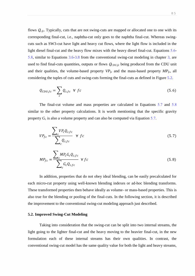
8 5

flows Qc,fc. Typically, cuts that are not swing-cuts are mapped or allocated one to one with its

corresponding final-cut, i.e., naphtha-cut only goes to the naphtha final-cut. Whereas swing-

cuts such as SW3-cut have light and heavy cut flows, where the light flow is included in the

light diesel final-cut and the heavy flow mixes with the heavy diesel final-cut. Equations 5.6-

5.8, similar to Equations 3.6-3.8 from the conventional swing-cut modeling in chapter 3, are

used to find final-cuts quantities, outputs or flows QCDU,fc being produced from the CDU unit

and their qualities, the volume-based property VPfc and the mass-based property MPfc, all

considering the tuples of cuts and swing-cuts forming the final-cuts as defined in Figure 5.2.

∑

( )

The final-cut volume and mass properties are calculated in Equations 5.7 and 5.8

similar to the other property calculations. It is worth mentioning that the specific gravity

property Gc is also a volume property and can also be computed via Equation 5.7.

∑

∑

( )

∑

∑

( )

In addition, properties that do not obey ideal blending, can be easily precalculated for

each micro-cut property using well-known blending indexes or ad-hoc blending transforms.

These transformed properties then behave ideally as volume- or mass-based properties. This is

also true for the blending or pooling of the final-cuts. In the following section, it is described

the improvement to the conventional swing-cut modeling approach just described.

5.2. Improved Swing-Cut Modeling

Taking into consideration that the swing-cut can be split into two internal streams, the

light going to the lighter final-cut and the heavy moving to the heavier final-cut, in the new

formulation each of these internal streams has their own qualities. In contrast, the

conventional swing-cut model has the same quality value for both the light and heavy streams,

8 6

which are the bulk or whole swing-cut properties VPc, Gc and MPc. In this work, it is

proposed a new swing-cut model that adds a set of interpolations to better predict the pooled

qualities of the final-cuts or products leaving the CDU or VDU. As mentioned before, it is

considered that both the light and heavy swing-cut streams have their own qualities, and are

computed as a function of their flows, and vary linearly or proportionately between the

properties at their adjacent hypothetical interfaces and the whole property of the swing-cut.

The properties of the adjacent hypothetical interfaces, between the swing-cuts and

their lighter and heavier cuts, can be easily calculated using the adjacent micro-cut pairs in the

initial and final boiling point temperatures of each swing-cut, taking into account CDU’s

crude diet to determine the micro-cut values. For instance, SW1-Cut in Figure 5.2 has its light

interface property variables as VPIc=SW1-Cut, and MPIc=SW1-Cut,, which are determined by

blending the mc120 and mc130 properties identical to Equations 5.4 and 5.5. Similarly, the

heavy interface properties VPIc=SW1-Cut,h and MPIc=SW1-Cut,h are computed using the micro-cuts

mc150 and mc160. This implies that the TBP temperature range for SW1-Cut has an initial

point of 130ºC and a final point of 160ºC, i.e., contains micro-cuts mc130, mc140, and

mc150.

As shown in Figure 5.4, the light and heavy swing-cut portions labeled SWL and

SWH have their properties varying between their adjacent hypothetical interface properties,

and its whole swing-cut property where the properties shown are volume-based but are the

same for mass-based. If the whole swing-cut flows entirely to the lighter final-cut then

VPc=sw,fc= is equal to the swing-cut bulk property VPc=sw. And, if all of the swing-cut flow

goes entirely to the heavier final-cut, then VPc=sw,fc=h = VPc=sw. In the cases where the swing-

cut is split to both the lighter and heavier product-cuts, then the properties are of course

different but related to the whole swing-cut property and have simple inequality constraints

bounding them, which may or may not be explicitly included in the model formulation.

8 7

Figure 5.4. Swing-cut properties as a function of light and heavy swing-cut flows.

Equations 5.9 and 5.10 are the equality constraints that allow to compute the light and

heavy swing-cut volume-based properties going to the light and heavy final-cuts, respectively,

where Equations 5.11 and 5.12 are for the mass properties using the specific-gravity variables.

( )

( )

and

( )

( )

With these equations, whole swing-cut properties VPc=sw and MPc=sw that can be

calculated by Equations 3.7 and 3.8 are replaced by VPc=sw,fc=, VPc=sw,fc=h, MPc=sw,fc= and

MPc=sw,fc=h which enables to predict more accurate mixed or pooled properties for the final

distillates. As shown in Figure 5.2, each swing-cut has light and heavy streams, and therefore

their properties can be corrected by this new improvement. Compared to the conventional

swing-cut method for the volume-based properties, four new variables are required

VPIc=sw,fc=, VPIc=sw,fc=h, VPc=sw,fc= and VPc=sw,fc=h, and two new equality constraints,

Lighter

Cut

Heavier

Cut

SWL

VPIsw,l

VPIsw,h

VPsw

VPsw,l

VPsw,h SWH

Lighter

Cut

Heavier

Cut

SWL

SWH

Lighter

Cut

Heavier

Cut

SWL

SWH

Lighter

Cut

Heavier

Cut

SWL

SWH

Lighter

Cut

Heavier

Cut

SWH

Lighter

Cut

Heavier

Cut

SWLQsw,l

Qsw,h

VPsw,l=VPsw VPsw,h=VPswVPsw,l ≤ VPsw

VPsw,h ≥ VPsw

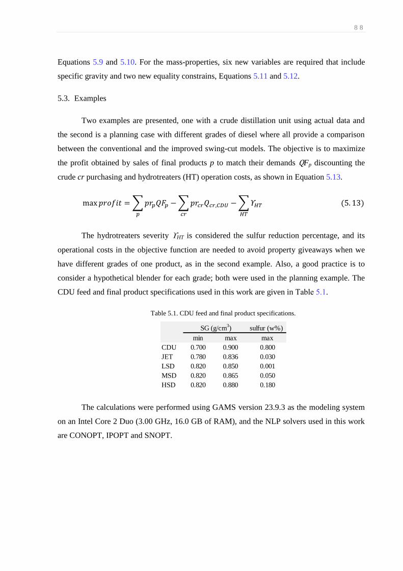
8 8

Equations 5.9 and 5.10. For the mass-properties, six new variables are required that include

specific gravity and two new equality constrains, Equations 5.11 and 5.12.

5.3. Examples

Two examples are presented, one with a crude distillation unit using actual data and

the second is a planning case with different grades of diesel where all provide a comparison

between the conventional and the improved swing-cut models. The objective is to maximize

the profit obtained by sales of final products p to match their demands QFp discounting the

crude cr purchasing and hydrotreaters (HT) operation costs, as shown in Equation 5.13.

∑

∑

∑

( )

The hydrotreaters severity HT is considered the sulfur reduction percentage, and its

operational costs in the objective function are needed to avoid property giveaways when we

have different grades of one product, as in the second example. Also, a good practice is to

consider a hypothetical blender for each grade; both were used in the planning example. The

CDU feed and final product specifications used in this work are given in Table 5.1.

Table 5.1. CDU feed and final product specifications.

The calculations were performed using GAMS version 23.9.3 as the modeling system

on an Intel Core 2 Duo (3.00 GHz, 16.0 GB of RAM), and the NLP solvers used in this work

are CONOPT, IPOPT and SNOPT.

sulfur (w%)

min max max

CDU 0.700 0.900 0.800

JET 0.780 0.836 0.030

LSD 0.820 0.850 0.001

MSD 0.820 0.865 0.050

HSD 0.820 0.880 0.180

SG (g/cm3)

8 9

5.4. Results

5.4.1. Example 1: CDU with three swing-cuts

This example involves an actual CDU operation with a capacity of approximately 35 k

m3 per day, and processes eighteen different crude oils, and their compositions are known and

fixed as shown in Table 5.2. The CDU configuration is shown in Figure 5.3 and has three

swing-cuts (SW1-Cut, SW2-Cut, and SW3-Cut) and four final-cuts (naphtha, kerosene, light,

and heavy diesel) of interest.

Table 5.2. Crude-oil diet with volume compositions.

In Figure 5.5 and Figure 5.6, we plot the specific gravity and sulfur profiles for each

CDU cut mentioned, where specific gravity is an example of a volume-based property. The

conventional swing-cut (CSW) calculations are displayed as the solid line with triangular

sample points ( ), whereas the improved swing-cut (ISW) values are displayed as the

dashed line with square sample points ( ). As expected, with the conventional method, the

light and heavy swing-cut properties are the same, which show as flat-lines for each swing-cut

pair. As proposed by the new and improved swing-cut method, the light and heavy swing-cut

crude º API SG (g/cm3) sulfur (%w) volume flow (m

3/d) volume rate (%)

Agbami 45.20 0.801 0.049 133 0.004

Akpo 44.96 0.802 0.066 2,444 0.069

Alcabora leste 20.26 0.932 0.562 3,624 0.102

Baz 28.54 0.884 0.271 2,428 0.068

Golfinho 26.91 0.893 0.152 339 0.010

Marlim leste jabuti 28.20 0.889 0.494 2,745 0.077

Marlim leste P-53 22.01 0.922 0.560 878 0.025

Marlim P-32 19.76 0.936 0.767 230 0.006

Marlim P-37 23.21 0.915 0.681 765 0.022

Marlim sul FPSO mls 23.59 0.912 0.599 13,569 0.383

Marlim sul P-40 22.98 0.916 0.638 168 0.005

Marlim sul P-51 21.05 0.928 0.639 986 0.028

Marlim sul P-56 18.01 0.946 0.727 565 0.016

Okono 40.61 0.822 0.057 1,556 0.044

Pennington 33.17 0.859 0.091 827 0.023

Roncador P-52 28.30 0.885 0.580 2,162 0.061

Roncador P-54 17.05 0.953 0.686 1,802 0.051

Saharan blend 43.47 0.809 0.071 237 0.007

total 35,458 1.000

9 0

properties are different from its whole or bulk swing-cut property and obey the varying

proportions shown in Figure 5.4.

Figure 5.5. Specific gravity for each CDU cut including the swing-cuts.

Figure 5.6. Sulfur content for each CDU cut including the swing-cuts.

Table 5.3 presents the CDU cuts volume flows determined when the throughput and

crude-oil diet are fixed as the final-cut amounts for naphtha (N), kerosene (K), and light diesel

(LD), which in this case are their final product demands, whereas Table 5.4 shows the

9 1

calculated specific gravity and sulfur property values for both the conventional and improved

swing-cut methods. Heavy diesel (HD) amounts are not fixed

Table 5.3. Flows for CDU cuts calculated and the given final-cuts used for both swing-cut methods.

Table 5.4. Specific-gravity and sulfur concentration for naphtha to heavy diesel cuts.

In Table 5.5, we highlight the final-cut specific gravity and sulfur properties that are

calculated using both the conventional and improved swing-cut models. These values are then

compared with actual data of a run performed on the CDU with the same total crude-oil flow

and diet as well as with naphtha, kerosene and light diesel final-cuts.

cuts final-cuts

cuts final-cuts

N 2.762

SW1L 0.446

SW1H 0.957

K 2.457

SW2L 1.027

SW2H 1.218

LD 2.444

SW3L 0.935

SW3H 1.564

HD 2.498HD -

LD 4.597

flow (k m3/d)

N 3.208

K 4.441

CSW ISW CSW ISW

N naphtha-cut

NI naphtha interface

0.765 0.753 0.016 0.014

0.765 0.769 0.016 0.021

KLI kerosene light interface

K kerosene-cut

KHI kerosene heavy interface

0.833 0.824 0.108 0.095

0.833 0.837 0.108 0.127

LDLI light diesel light interface

LD light diesel-cut

LDHI light diesel heavy interface

0.869 0.866 0.316 0.278

0.869 0.873 0.316 0.343

HDI heavy diesel interface

HD heavy diesel-cut

0.220

0.344

0.453

sulfur (%w)

0.894

swing-cut 3

0.882

0.799

0.817

0.747

SW2-cut swing-cut 2

0.842

SW1-cut swing-cut 1

0.852

0.860

SW3-cut

0.777 0.024

SG (g/cm3)

0.711 0.006

0.009

0.055

0.068

0.127

0.195

9 2

Table 5.5. Specific-gravity and sulfur concentration values for both swing-cut methods.

From Table 5.4, the specific gravity predictions using the improved swing-cut method

show marginally better agreement with the actual plant data compared with the conventional

swing-cut method, although the conventional method is still within experimental error. For

the sulfur predictions the data is more inconclusive in terms of which method is better. As for

this example all crude oils are fixed and also for the final product demands of naphtha,

kerosene and light diesel, the case is treated as a simulation because the number of variables

and equations are the same, so there are no degrees of freedom. In the next example, the

difference in qualities predictions for both swing-cuts models is shown in an optimization

case for the operational planning considering different grades of diesel as like as hydrotreaters

operation.

5.4.2. Example 2: oil-refinery planning case

Four crude oils are used, and the CDU diet is determined considering property

specifications on the final products and the processing taking place in the CDU and

hydrotreaters as shown in Figure 5.7. The sulfur reduction provided by the hydrotreaters is a

variable controlled by their severity where the bounds are given by Equations 5.14 and 5.15.

( )

( )

final-cuts N K LD N K LD

Conventional Swing-Cut (CSW) 0.719 0.800 0.849 75 600 1980

Improved Swing-Cut (ISW) 0.717 0.798 0.852 78 570 1950

Actual Plant Data 0.717 0.797 0.862 105 503 2354

SG (g/cm3) sulfur (wppm)

9 3

Figure 5.7. Fuels production planning case.

The final products or pooled demands are completely free or open so that the

optimization problem can determine the crude-oil diet and maximize the profit considering

the quality constraints for the CDU feeds and product fuels. Table 5.6 shows the results for

the profit, unit throughputs, and final product amounts for the conventional (CSW) and

improved (ISW) swing-cut models where the proposed model predicts an improvement in the

profit of 3.3% (12.0 k US$/d or 4.380 million US$/y).

Kerosene

Light Diesel

ATR

CDU

C1C2

C3C4

SW1

SW2

SW3

VR

VDU

N

K

LD

HD

D1HT

Naphtha

Heavy Diesel

LVGO

HVGO HTD2

D2HT

HTD1

to hydrotreating

and/or reforming

(To FCC)

Crude C

Crude D

(To Delayed Coker)

to hydrotreating

to caustic and

amines treating

JET

GLN

FG

LPG

VGO

FO

Final Products

MSD

HSD

LSD

Crude A

Crude B

9 4

Table 5.6. Planning example results.

Table 5.7 and Table 5.8, the cuts (also swing-cuts) and the final pool properties

explain the different production amounts for JET and the distillates using CSW and ISW

methods. Because the JET has the higher price and there are only property constraints in the

model, the lower light-SW2 sulfur content in the ISW model enables higher flow of this

stream to the kerosene final-cut (sulfur content specification ≤ 0.030%) and hence a higher

profit is achieved. In Table 5.8 all sulfur content specification in the products are at their

maximum value, without giveaway in quality.

units (m3/d) CSW ISW lower upper

CDU 18,000 18,000 14,000 18,000

VDU 9,960 9,960 6,000 10,000

D1HT 1,000 1,000 500 1,000

D2HT 2,200 2,200 1,000 2,200

hydrotreaters severity

D1HT 0.950 0.950 0.920 0.950

D2HT 0.995 0.995 0.950 0.995

crude (m3/d)

A 2,060 2,060

B 15,940 15,940

C

D

fuels (m3/d)

FG 8 8

LFG 213 213

GLN 1,478 1,478

JET 2,214 2,330

LSD 1,764 1,966

MSD 1,890 1,349

HSD 473 697

VGO 4,721 4,721

FO 5,239 5,239

profit (k US$/d)

367.8 379.8

273.0

681.5

800.0

708.0

550.0

498.0

693.8

680.0

price (US$/m3)

720.0

price (US$/m3)

540.0

585.0

569.0

9 5

Table 5.7. Cuts flows and properties.

Table 5.8. Specific-gravity and sulfur concentration in the CDU feed and final pools.

The size of the problem is relatively small given that we are not including the entire oil

refinery, and there is only one time period that has been considered. Table 5.9 and Table 5.10

show the model sizes and also the results for the solvers CONOPT, SNOPT, and IPOPT.

Table 5.9. Models sizes.

Table 5.10. Solvers results.

The modest increase in the number of extra variables, constraints, and nonzeros for the

improved swing-cut method should not significantly increase the computational time when

cuts final-cuts CSW ISW CSW ISW CSW ISW

LN LN

SW1L - - 0.765 0.756*

0.005 0.003*

SW1H K 679 679 0.765 0.765 0.005 0.005

K

SW2L 293 409 0.828 0.819 0.074 0.062

SW2H LD 825 709 0.828 0.833 0.074 0.088

LD

SW3L - - 0.867 0.858*

0.272 0.217*

SW3H HD 911 911 0.867 0.867 0.272 0.272

HD*properties at the interfaces

0.380

1,242 0.794 0.032

1,490 0.848 0.148

cuts flows (m3/d) SG (g/cm

3) sulfur (w%)

1,478 0.714 0.001

902 0.887

CSW ISW CSW ISW

CDU 0.900 0.900 0.459 0.459

JET 0.789 0.790 0.030 0.030

LSD 0.850 0.850 0.001 0.001

MSD 0.858 0.861 0.050 0.050

HSD 0.877 0.877 0.180 0.180

sulfur (w%)SG (g/cm3)

CSW ISW

equations 154 194

variables 173 213

nonzeros 592 756

nonlinear 317 449

CSW ISW CSW ISW CSW ISW

CONOPT 0.219 0.062 213 188 367.8 379.8

IPOPT 0.156 0.234 105 162 367.8 379.8

SNOPT 0.047 0.078 23 16 367.8 379.8

CPU (s) profit (k US$)iteration

9 6

embedded into larger planning or scheduling optimization problems. Good initial starting

points for the variables can also be determined by first solving the conventional swing-cut

model followed by the improved swing-cut model. In our opinion, the added accuracy

afforded by the improved swing-cut method will more than offset the slight increase in

solution time that may be required.

5.5. Conclusions

We have presented in this chapter a new and relatively simple improvement to the

conventional swing-cut modeling found in most nonlinear planning and scheduling

optimization models used to plan and schedule most of the world's oil refineries. The concept

is simple, in the sense that the usual assumption that the swing-cut properties flowing from

the swing-cut to the light and heavy final-cuts (or product-cuts) are the same, has been

extended or modified to account for the fact that they vary according to their proportions

between the light and heavy interfaces. This can be easily calculated using the bilinear

equations in Equations 5.9 to 5.12. A small but representative example, taken from an actual

CDU operation with eighteen crude oils and three swing-cuts (see Figure 5.3), was

highlighted to demonstrate the property differences for the light and heavy swing-cut streams

in both methods. Also, a planning example with different grades of diesel, including two

hydrotreater operations, shows that the improved swing-cut model yields higher profit

because of its higher jet fuel production, provided by the lower specific gravity value for the

light-SW2 flowing to the kerosene final-cut. Conceptually, the notion that the light and heavy

flows from the swing-cut to its corresponding light and heavy final-cuts have different

properties is sound engineering and was shown qualitatively to be acceptable with respect to

the results shown. The improved swing-cut method can choose the best solution considering

the more accurate formulation, and even if the problem presented lower profit for a specific

set of constraints, the improved method avoids the overestimation of the profit.

9 7

Chapter 6

in Kelly, J.D.; Menezes, B.C.; Grossmann, I.E. Distillation Blending and Cutpoint

Temperature Optimization using Monotonic Interpolation. Industrial & Engineering


6. Distillation Blending and Cutpoint Temperature Optimization using

Monotonic Interpolation

A novel technique using monotonic interpolation to blend and cut distillation temperatures

and evaporations for petroleum fuels in an optimization environment is proposed. Blending

distillation temperatures are well known in simulations whereby cumulative evaporations at

specific temperatures are mixed together these data points are used in piece-wise cubic spline

interpolations to revert back to the distillation temperatures. Our method replaces the splines

with monotonic splines to eliminate Runge's phenomenon, and to allow the distillation curve

itself to be adjusted by optimizing its initial and final boiling points known as cutpoints. By

optimizing both the recipes of the blended material and its blending component distillation

curves, very significant benefits can be achieved especially given the global push towards

ultralow sulfur fuels (ULSF), because of the increase in natural gas plays reducing the

demand for other oil distillates. Four examples are provided to highlight and demonstrate the

technique.

6.1. Introduction

Oil refinement involves a series of complex manufacturing processes in which the

final products (such as fuels, lubricants, and petrochemical feedstocks) are produced from

crude-oil feedstocks by separation and conversion unit-operations, in coordination with tanks,

blenders, and transportation vessels. To manage the processing of the hydrocarbon streams,

well-known distillation curves or assays of both the crude-oil and its derivatives are

decomposed or characterized into several temperature “cuts”, based on what are known as the

True Boiling Point (TBP) temperature distribution or distillation curves (Riazi, 2005), and can

be found in all process design simulators and crude-oil assay management programs. These

curves are relatively simple and one-dimensional representations of how a complex

hydrocarbon material’s yield and quality data (such as density, sulfur, and pour point) are

9 8

distributed or profiled over its TBP temperatures, where each cut is also referred to as a

component, pseudo-component, or hypothetical in process simulation and optimization

technology. Throughout the oil-refinery process, the full range of hydrocarbon components is

transformed (blended, reacted, separated) to smaller boiling-point temperature ranges,

resulting in intermediate and final products in which planning and scheduling optimization

using TBP curves of the various streams can be used to effectively model these process unit-

operations and predict the macroscopic (i.e., cold flow) properties of their outlet streams

(Kelly, 2004). The entire refining process can be categorized into three distinct areas: crude-

oil blending, refinery unit-operation processing, and product blending (Jia et al., 2004), where

the focus is related to the last two areas.

Our proposed new technique is to integrate both the optimization of blending several

streams’ distillation curves together with also shifting or adjusting the cutpoints of one or

more of the stream’s initial boiling point (IBP) and/or final boiling point (FBP) in order to

manipulate its TBP curve in an either offline or online environment. This shifting or adjusting

of the TBP curve’s IBP and FBP (front end and back end respectively) ultimately requires that

the upstream unit-operation has sufficient handles or controls to allow this type of cutpoint

variation, where the solution from this higher-level optimization would provide set points or

targets to lower-level advanced process control systems, which are now commonplace in oil

refineries. By shifting or adjusting the front end and back end of the TBP curve for one or

more distillate blending streams, it allows for improved control and optimization of the final

product demand quantity and quality, affording better maneuvering closer to and around

downstream bottlenecks, such as tight property specifications and volatile demand flow and

timing constraints.

These distillate blending streams are usually produced from divergent and

multiproduct distillation towers (e.g., atmospheric and vacuum distillation columns

(CDU/VDU) and fluid catalytic and hydrocracking main fractionators (FCCU/HCC)); thus,

changes in the yields and properties of one stream results in changes in the adjacent streams.

Physical phenomena that are related to these changes are described by molar, energy, and

equilibrium balances, etc. and are significantly influenced by the tower’s operating or

processing conditions, such as temperature and pressure profiles, as well as its feed

composition. Modeling and solving these types of phenomena would require sophisticated

process design caliber and rigorous simulation software, which has its own and well-

recognized set of difficulties for the type of industrial implementation used here. Instead, our

9 9

approach is simpler, whereby we adjust and interpolate actual measured data of the

evaporation curves to optimize, based on downstream product blending demand flows and

qualities by manipulating recipes at the blend headers and incrementally shifting initial and

final cutpoints (IBP and FBP) of the upstream rundown components when required to

alleviate certain bottleneck constraints encountered during the downstream blending. These

new recipes and IBP/TBP cutpoints then become targets that are sent to advanced and

regulatory process controllers. The benefits for such an optimization strategy can be found in

a recent white paper by Honeywell (Honeywell, 2014), which has a payback of less than one-

month at an European oil-refinery producing a majority of its products as diesel fuel, while

similar benefits for crude-oil blend scheduling optimization can be found documented in the

report by Kelly and Mann (2003a, 2003b).

6.2. Distillation Curve Overview

Hydrocarbon streams (crude oils, fuels, petrochemical feeds) are identified or

characterized by distillation curves, in terms of their quantity (yield) and quality (properties)

and how they vary with respect to temperature. These data are determined by experimental

methods using small-scale laboratory distillation columns in which hydrocarbon fractions are

collected at certain boiling-point temperatures to define their quantity and quality data or

assay at each boiling temperature. These data can then be used in mathematical models, either

in rigorous engineering or simplified empirical simulation and optimization environments, to

determine the yields and properties of distillation, separation, or fractionation unit-operation

outputs. Integrated with this can be the final product recipes necessary to match demand

quantity and quality specifications such as specific gravity, sulfur, pour point, and evaporation

temperatures of the fuels, so that simultaneous distillation blending and cutpoint temperature

shifting or adjusting can be simulated and optimized together, as is proposed in this work.

Since obtaining TBP curve data directly from a laboratory distillation run is expensive

and time-consuming, the normal procedure is to determine distillation curves by applying

American Society for Testing and Material (ASTM) methods such as D86 (atmospheric) and

D1160 (vacuum) or simulated distillation (SD) methods, using gas chromatography (GC)

such as D2887 and D7169. These are based on reduced numbers of separation stages and can

fortunately be easily interconverted to TBP data with sufficient accuracy and precision (Riazi,

2005). Figure 6.1 shows both the ASTM D86 and TBP data from the Colorado School of

1 0 0

Mines (2012) for a straight-run gasoline stream from a crude-oil distillation unit (CDU),

plotted with volume yield percent as the ordinate and temperature as the abscissa.

Figure 6.1. ASTM D86 and TBP volume yield percent curves.

A well-known observation, with regard to Figure 6.1, is that the ASTM D86 and TBP

temperatures are near equal at their 50% yield point, whereas D86 yields are underestimated

below the 50% yield and D86 yields are overestimated above the 50% yield. Equations 6.1 to

6.13 are the Riazi correlations used to convert ASTM D86 (D01 to D99) to TBP (T01 to T99)

temperatures at conventional yield percentages of 1%, 10%, 30%, 50%, 70%, 90%, and 99%,

where the same equations can be simply inverted in order to convert from TBP to ASTM

D86.

( ) ( )

( ) ( )

( ) ( )

( ) ( )

( ) ( )

1 0 1

( ) ( )

Equations 6.1 to 6.6 use the differences between the ASTM D86 temperatures to

compute TBP temperature differences at the same percent yields, where Equations 6.7 to 6.13

use the TBP temperature at 50% yield to difference backward and forward to the other TBP

temperatures.

( )

( )

( )

( )

( )

( )

( )

Note that for the IBP and FBP, we use the percent evaporated at 1% and 99% instead

of 0% and 100%; this is a well-known recommendation found in several sources, given then

repeatability of the 1% and 99% evaporated when compared to the 0% and 100%

counterparts. Other interconversion correlations can be found Riazi and Daubert (1986) and

Daubert (1994). Also note that, for temperatures greater than circa 650 ºF, and at atmospheric

pressure, thermal cracking may occur due to pyrolysis reactions. In these situations, ASTM

D1160 should be used, which is conducted at a lower pressure (near vacuum), where its

temperatures need to be corrected back to atmospheric pressure.

For product streams separated from unit-operations such as distillation columns and

fractionation towers, the experimental TBP and/or ASTM distillation curves reflect the

nonideal separation inside the vessels. For example, if we compare a CDU’s crude-oil feed

distillation curve with all of its product distillation curves, as shown in Figure 6.2, it is

interesting to see what are known as overlaps between the light and heavy adjacent products;

this represents what is referred to as nonsharp or nonideal fractionation (Li et al. 2005).

1 0 2

Figure 6.2. Feed and product yield curves.

These overlaps are due to the limitations in the number and efficiency of the

equilibrium stages in the column, as well as the reflux ratios when operating the actual tower.

In general, the separation temperature between two adjacent fractions is called the

temperature cutpoint and is defined by Watkins (1979) as the midpoint of the TBP

overlapping temperatures; this parameter has been used in previous studies, such as the works

of Li et al. (2005), Guerra and Le Roux (2011a, 2011b), and Alattas et al. (2011, 2012).

In another study by Mahalec and Sanchez (2012), they used two models: one is a PLS

model which infers product composition from some of the tray temperatures which is similar

to Mejdell and Skogestad (1991), while the second model computes product yields from

internal reflux and cutpoint temperatures which requires data to be generated from rigorous

process simulations to develop the hybrid models.

1 0 3

6.3. Distillation Blending using Monotonic Interpolation

In an industrial fuels blending optimization problem, starting recipes or ingredient

amounts to produce hopefully on-specification final products are based on mixing

intermediate products or components with somewhat known quantity availabilities and

laboratory- and/or field-analyzed qualities. However, there will be some component quantity

and quality variability or uncertainty over the duration of the blend which is attenuated to

some degree when dead or standing-gauge component tanks are used to decouple the

upstream processing from the downstream blending (Kelly, 2006). As such, in most oil-

refinery blendshops today, real-time nonlinear model-based advanced process controllers are

used to control the final blended product qualities, incorporating online measurement

feedback from diverse online analyzers and usually projecting one and perhaps two time

periods into the future. Their manipulated variables are the recipes or ratio amounts of

components directly feeding into the blender, which are transferred as set points to basic

regulatory PID controllers. In this study, our focus is the off-line optimization of the initial

recipes sent down to the online control strategy, although it would be straightforward to

optimize in real-time provided that measurement feedback is also included similar to bias

updating or moving horizon estimation employed in advanced process (Forbes and Marlin,

1994; Kelly and Zyngier, 2008).

The difficulty with blending the distillation temperatures from several component

materials is that these TBP distillation temperatures do not blend linearly on a mass or volume

basis. Although there is some use of what are commonly referred to as blending indices or

property transforms for distillation temperatures (and used effectively for other properties

such as cloud-point, pour point, viscosity, etc.), which then allow the indexed or transformed

properties to be blended linearly, literature on their mathematical structure and coefficients is

scarce. Instead, an acceptable approach is to convert the TBP temperatures to evaporation

cumulative compositions at several pre-defined temperatures using monotonic interpolation of

which linear interpolation is inherently monotonic but may not be as accurate as higher-order

monotonic interpolations (Fritsch and Carlson, 1980; Fritsch and Butland, 1984; Kruger,

2002). Unfortunately, if nonmonotonic interpolation is used such as cubic splines, then

oscillating behavior around the breakpoints will occur; this is well-known as Runge’s

phenomenon. The temperature range should be defined to span all of the expected TBP

temperatures for all of the distillates included in the blend at a suitable level of resolution or

1 0 4

temperature discretization. After the set of evaporation components have been blended

together using the recipes fractions of each component blended, the blended product’s

distillation temperatures at 1%, 10%, 30%, 50%, 70%, 90% and 99% evaporated, distilled or

yielded are computed by again using monotonic interpolation where the evaporation

components constitute the abscissa and the distillation temperatures represent the ordinate.

Monotonic interpolation is defined as a variant of cubic interpolation that preserves

monotonicity of the dataset being interpolated. Monotonicity is maintained by linear

interpolation but not guaranteed by cubic interpolation (Wikipedia, 2014). As observed in

both Figure 6.1 and Figure 6.2, distillation curves are inherently monotonic; therefore, not

using monotonic interpolation will result in unrealistic and unexpected prediction variability.

Although linear interpolation will produce monotonic interpolations it does not preserve the

shape of the curves. Shape-preserving cubic splines are available known as Piecewise Cubic

Hermite Interpolation Polynomials (PCHIP) (Fritsch and Carlson, 1980; Fritsch and Butland,

1984; Kahaner et al., 1988; Kruger, 2002). More recently, another shape-preserving or what

has been termed “constrained” cubic spline interpolation method has appeared; this method

was developed based on practical arguments by Kruger (2002) and employed in the financial

sector for bond yields, for example (Greeff, 2003).

To summarize, the overall calculation process of distillation blending is shown in

Figure 6.3. We first interconvert from ASTM D86 to TBP temperatures, and using the TBP

temperatures at their defined yields of 1%, 10%, 30%, etc., evaporations are determined by

interpolating the TBP distillation curve at selected predefined TBP temperature increments.

These evaporation cumulative compositions for each blending component are mixed using the

ideal blending law, i.e., no excess properties and no nonlinear behavior, where, if the amounts

or flows of components are fixed, then this is also called linear blending.

1 0 5

Figure 6.3. Flowchart of distillation blending calculation process.

After the blending of all of the components’ evaporations, another interpolation step is

used to compute the TBP temperatures of the final blended product at the defined yield

values. Then, interconversion is again used to calculate the ASTM D86 temperatures, which

can be downloaded to various control strategies, as mentioned.

6.4. Cutpoint Temperature Optimization

Distillation curves of petroleum products are typically plotted as TBP temperature

versus relative yield percent, where we have chosen to represent the curves in the opposite

way, indicating that the TBP temperature is now our independent variable or degree-of-

freedom in the optimization. When yields, evaporations, or relative amounts distilled of the

distillates are used as a function of temperature, the IBP (T01) and FBP (T99) can be

manipulated for example to adjust or shift the distillation curve by interpolation and/or

extrapolation in order to increase or decrease the front end and back end of the curves, as

graphically depicted in Figure 6.4. The incremental or marginal adjustment or shifting can

also be likened to fine-tuning the distillation curve, and this will ultimately translate to

changing all of the relative yield values along the total or overall TBP temperature range of

the distillate stream. This will have the desired effect that we can alter the evaporation

amounts in the downstream blending to better control and optimize the blend quantity and

quality specifications to meet market demands. However, when we manipulate the T01 and/or

T99 for any distillate component stream, these values (interconverted to D01 and D99, if

required) must be sent down as targets or set points to an appropriate advanced process

ASTM D86

TBP

Inter-conversion

Evaporation

Curves

Interpolation

Ideal Blending

Evaporation

Curve

Multiple

Components

Final

Product

ASTM D86

Interpolation

Inter-conversion

TBP

1 0 6

control strategy on the respective upstream unit-operation such as an atmospheric crude-oil

distillation column or the main fractionator tower of the fluidized bed catalytic cracking unit

(FCCU). Fortunately, such strategies are available whereby reliable online analyzers measure

in real-time or near-time (including sampling and analysis delays) ASTM D86 temperatures,

which can be linked to pump-around heat exchanger duty and draw tray temperature controls

to achieve the desired increase and/or decrease in initial and final cutpoint temperatures.

Figure 6.4. Distillation curve adjustment or shifting, as a function of TBP temperature.

Our new distillation curve adjustment or shifting technique to perform temperature

cutpoint optimization is straightforward to implement mathematically. The concept is to

assume that a typical distillation curve can be reasonably decomposed or partitioned into three

distinct regions or parts, i.e., a front end, a middle, and a back end. The different sections can

be sufficiently approximated as straight lines or piece-wise continuous from OT01 to OT10

for the front end, OT10 to OT90 for the middle, and OT90 to OT99 for the back end, where

“O” stands for “old” and, of course, “N” stands for “new” (for the new adjusted or shifted 1%

and 99% temperatures found in Equations 6.14 to 6.17, i.e, NT01 and NT99).

Equations 6.14 and 6.15 model both the yield (YNT01) and the change or difference in

the yield (DYNT01) when we adjust or shift T01 from OT01 to NT01, assuming a constant

1 0 7

slope determined from the unadjusted or unshifted old/original curve. Obviously, if NT01 =

OT01 (no change), then YNT01 = 0.01 and DYNT01 = 0.0, as expected.

( ) ( )

( )

Similarly, for the back-end regime, we can model the new yield at NT99 and its delta

yield DYNT99 in Equations 6.16 and 6.17, respectively. Morover, if NT99 = OT99, then

YNT99 = 0.99 and DYNT99 = 0.0, trivially.

( ) ( )

( )

Equation 6.18 easily models the increase or decrease in the new flow from the

upstream unit-operation, depending on the amount of adjustment or shifting of the cutpoint

temperature variables NT01 and NT99, where OF denotes the old or measured flow value.

( ) ( )

A useful feature of adjusting or shifting the distillation curve, along the original front-

and back-end slopes, is its ability to predict the marginal increase or decrease in the distillate

stream flow directly without having to resort to a separate equation with unknown coefficients

that will need to be continuously calibrated.

Given that our TBP distillation curve plots the relative yield versus temperature, we

need to normalize each new yield found in Equations 6.19 to 6.25 which correspond to the

temperatures NT01, OT10, OT30, OT50, OT70, OT90, and NT99. Again, if both DYNT01 =

DYNT99 = 0.0, because NT01 = OT01 and NT99 = OT99, then we are obviously left with our

old or original TBP distillation curve for the upstream unit-operation component distillate

stream yield profile.

( )⁄ ( )

( ) ( )⁄ ( )

( ) ( )⁄ ( )

1 0 8

( ) ( )⁄ ( )

( ) ( )⁄ ( )

( ) ( )⁄ ( )

( ) ( )⁄ ( )

The idea for these equations is straightforward, in the sense that if we increase or

decrease the front end and the back end, then given their delta yield amounts found in in

Equations 6.15 and 6.17, we can easily adjust the new yields, given the old yields where the

old yields are, of course, the well-defined 1%, 10%, 30%, etc. values. However, it is re-

emphasized that our approach is to incrementally or marginally shift or adjust the NT01 and

NT99 so as not to significantly disrupt the adjacent distillation streams and can be controlled

by specifying acceptable bounds on NT01 and NT99 in the optimization.

Also, it should be pointed out that our use of the term cutpoint is somewhat different

than is found, for example, in the work of Mahalec and Sanchez (2012) and chapter 5, in

which a cutpoint is defined as the lower/initial and upper/final temperatures on the TPB of the

entire crude oil, which hypothetically represents the crude-oil fraction distilled or evaporated

from the distillation tower such as a CDU. Instead, given that the TBP curve of a CDU’s

crude-oil mixture is not normally available in practice, and especially if the feed is to an FCC

main fractionator, which is rarely known, we use the definition commonly found in oil-

refinery operations (Honeywell, 2014) of defining cutpoint temperatures as the smallest

and/or largest controllable separation or fractionation temperature (i.e., IBP, 5% or 10% and

90%, 95%, or FBP) between adjacent cuts, fractions, or streams from a distillation tower.

6.5. Examples

Four examples are provided below, which are modeled and solved using IMPL

(Industrial Modeling and Programming Language) from Industrial Algorithms LLC. IMPL is

a problem-specific platform suitable for both discrete and nonlinear process industry

optimization problems and implements monotonic interpolation as standard built-in functions,

whereby all first-order partial derivatives are computed numerically but close to analytical

quality (Squire and Trapp, 1998). Other modeling systems such as GAMS and AIMMS

unfortunately do not provide derivatives automatically for the variables found in both the

1 0 9

abscissa and ordinate axes of the interpolation dataset. Another detail of the implementation

in IMPL is the use of ranking, ordering, or precedence constraints to ensure that the abscissa

data used in the interpolation is in ascending or increasing order, especially when the x-axis

can be composed of variables. These are simple linear inequalities that enforce that the TBP

temperature for, e.g, a 10% yield is less than or equal to its adjacent TBP temperature at 30%;

these ranking constraints are also applied to the cumulative evaporations. Furthermore, to

generate useful initial values or starting points for the optimization, IMPL also has simulation

capability when the degrees-of-freedom equal zero (i.e., all component flows are fixed or

known) whereby the sparse Jacobian matrix is iteratively factorized (using various LU

decompositions) and successive substitution is employed to cycle to a solution. To locally

solve the resulting nonlinear and nonconvex problem, IMPL employs a typical or standard

successive linear programming (SLP) algorithm (Zhang and Lasdon, 1985) called SLPQPE,

which is also not available in the GAMS and AIMMS but is very appropriate for these types

of problems.

6.5.1. Example 1: Gasoline blending simulation

This is a gasoline or naphtha blending simulation case taken directly from a

presentation on oil-refinery feedstock and product property modeling from Colorado School

of Mines (2012). It is a 50:50 mixture of two gasoline components - LSR (light straight run)

and MCR (midcut reformate) - with ASTM D86 (1 atm) of [(1%,91), (10%,113), (30%,121),

(50%,132), (70%,149), (90%,184), (99%,258)] and [(1%,224), (10%,231), (30%,232),

(50%,234), (70%,237), (90%,251), (99%,316)], respectively, where the temperatures are

expressed in degrees Fahrenheit (ºF). Again, we are using their recommendation to consider

the IBP and FBP temperatures to be defined at 1% and 99% instead of 0% and 100%, of

course, which in practice, are difficult to measure. Converting these to TBP temperatures

(also at 1 atm) using the method defined by Riazi (2005) (see pages 103-104, equations 3.20,

3.21, 3.22 and Table 3.7), we get values of [(1%,40.5), (10%,88.1), (30%,109.9),

(50%,130.5), (70%,156.3), (90%,200.9), (99%,350.8)] and [(1%,200.8), (10%,224.7),

(30%,229.6), (50%,234.8), (70%,241.1), (90%,263.4), (99%,384.2)], respectively, which are

identical to the results from Colorado School of Mines.

When we interpolate from the interconverted TBP temperatures to evaporation

cumulative fractions using the three different monotonic interpolation methods (linear,

1 1 0

PCHIP, and Kruger), we get the following results found in Table 6.1 and Table 6.2, along

with the results from Colorado School of Mines, where Figure 6.5 plots LSR’s interpolated

evaporation cumulative compositions using the data from Table 6.1 and LSR’s TBP curve

data.

Table 6.1. Example 1’s Interpolated Evaporation Fraction Results for LSR.

Figure 6.5. Example 1’s LSR interpolated yield (%) versus TBP temperature.

Colorado Linear PCHIP Kruger

E25 0.004 0.006 0.004 0.005

E50 0.017 0.028 0.017 0.017

E75 0.058 0.075 0.061 0.063

E100 0.193 0.209 0.195 0.194

E125 0.444 0.447 0.449 0.449

E150 0.654 0.651 0.659 0.659

E175 0.800 0.784 0.807 0.807

E200 0.897 0.896 0.899 0.899

E225 0.926 0.914 0.927 0.924

E250 0.948 0.929 0.948 0.944

E275 0.964 0.944 0.964 0.961

E300 0.976 0.959 0.976 0.974

E325 0.984 0.975 0.985 0.984

E350 0.990 0.990 0.990 0.990

E375 0.994 0.992 0.994 0.994

E400 0.996 0.995 0.997 0.996

1 1 1

It should be noted that the distillation temperature at the 10% yield point appears to be

more off the curve than the others. Its deviation can be reduced by increasing the number of

evaporation points used in the monotonic interpolation, although at the expense of increasing

the number of points to be calculated in the simulation or optimization.

Table 6.2. Example 1's Interpolated Evaporation Fraction Results for MCR.

After we have blended the evaporation fractions using a recipe of 50% LSR and 50%

MCR, Table 6.3 shows the results using the three monotonic interpolation methods

interconverting from TBP to ASTM D86 temperatures.

Table 6.3. Example 1: Interconverted ASTM D86 (TBP) Temperatures in ºF.

Based on the temperature data, the interpolation method used by Colorado School of

Mines seems to be more of a cubic spline method than a linear interpolation method, given


E25 0.000 0.001 0.000 0.001

E50 0.000 0.002 0.003 0.001

E75 0.000 0.004 0.001 0.002

E100 0.000 0.005 0.002 0.003

E125 0.000 0.006 0.003 0.004

E150 0.000 0.007 0.005 0.006

E175 0.000 0.009 0.007 0.008

E200 0.009 0.010 0.010 0.010

E225 0.110 0.114 0.104 0.104

E250 0.796 0.780 0.817 0.813

E275 0.917 0.909 0.918 0.915

E300 0.945 0.927 0.948 0.942

E325 0.965 0.946 0.968 0.963

E350 0.979 0.965 0.980 0.978

E375 0.988 0.983 0.988 0.987

E400 0.993 0.992 0.994 0.993


1% 120.5 (52.9) 109.0 (38.6) 120.0 (52.7) 118.8 (51.2)

10% 142.8 (101.0) 140.2 (97.4) 142.1 (100.5) 142.0 (100.4)

30% 163.6 (144.0) 162.6 (142.9) 161.6 (141.7) 161.4 (141.5)

50% 217.7 (218.0) 218.8 (219.2) 220.7 (221.1) 221.3 (221.8)

70% 228.6 (236.0) 230.8 (238.6) 230.4 (237.5) 230.7 (237.7)

90% 242.9 (258.7) 248.9 (265.7) 239.8 (254.0) 241.0 (255.3)

99% 305.3 (371.7) 313.2 (384.4) 303.7 (371.3) 304.9 (372.8)

1 1 2

that they did not specify what type of interpolation method they used. The two monotonic

cubic spline methods (PCHIP and Kruger) have comparable results to the first column

(Colorado), especially when we consider the quoted ± 9 ºF (± 5 ºC) precision of the Riazi

method (page 104) (Riazi, 2005). Therefore, we can conclude that depending on the

interpolation method, different ASTM D86 interconversion temperatures can result for the

same evaporation or distilled composition amounts.

Table 6.4 shows Example 1’s model statistics using SLPQPE with IBM’s CPLEX 12.6

as the LP subsolver on an Intel Core i7 2.2 GHz laptop computer.

Table 6.4. Example 1: Statistics.

6.5.2. Example 2: Diesel blending and cutpoint temperature optimization

This case is taken, in part, from Erwin (1992), in terms of using his ASTM D86 (1

atm) temperatures for his four experimental diesel components (DC1-DC4), as shown in

Table 6.5 and Figure 6.6, where the dotted line represents the final product blend distillation

curve.

Table 6.5. Example 2: InterConverted TBP (ASTM D86) Temperatures in ºF.

equality constraints 107

inequality constraints 135

variables 108

equality non-zeros 672

inequality non-zeros 270

DC1 DC2 DC3 DC4

1% 305.2 (353) 322.2 (367) 327.0 (385) 302.4 (368)

10% 432.9 (466) 447.1 (476) 405.2 (435) 369.7 (407)

30% 521.6 (523) 507.1 (509) 457.1 (462) 441.0 (449)

50% 565.3 (551) 549.5 (536) 503.3 (492) 513.8 (502)

70% 606.4 (581) 598.4 (573) 551.1 (528) 574.3 (550)

90% 668.3 (635) 666.1 (634) 605.8 (574) 625.4 (592)

99% 715.7 (672) 757.7 (689) 647.0 (608) 655.2 (620)

1 1 3

Figure 6.6. Example 2’s TBP distillation curves, including the final blend.

Our blending and cutpoint temperature optimization objective function is to maximize

the flow of DC1 and DC2, subject to their relative and arbitrary pricing of 0.9 for DC1 and

1.0 DC2, with lower and upper bounds of 0.0 and 100.0 each. For simplicity, we have fixed

each of the flows for DC3 and DC4 to a marginal and arbitrary value of 1.0, and the total

blend flow cannot exceed 100.0. The typical ASTM D86 temperature specification for

international diesel sales is D10 ≤ 480, 540 ≤ D90 ≤ 640, and D99 ≤ 690 ºF. To make this

problem more interesting, we have set the bounds to D10 ≤ 470, 540 ≤ D90 ≤ 630 and D99 ≤

680. This ensures that it is not possible to satisfy the diesel blend with the most valuable DC2

component as its D10, D90, and D99 temperatures are all greater than our blended diesel's

distillation temperature specification. Furthermore, it is also not possible to fill the blend with

all DC1, because its D90 does not comply with the specification. As such, this forces a

mixture of DC1 and DC2 and as we shall see, this also requires an adjustment or shifting to

the distillation curve for DC1 where only the DC1 material is allowed to have manipulated

cutpoint temperatures. At the optimized solution, NT01 = 312.8 and NT99 = 689.3, which are

both different than their original values of OT01 = 305.2 and OT99 = 715.7. Since both their

front- and back-end temperatures have been reduced, we expect that the new flow for DC1 is

less than the old flow and it is NF = 37.06 and OF = 39.24; consequently, the flow for DC2 is

1 1 4

60.94 which is consistent with the total flow of 100.0. The new and optimized TBP curve for

DC1 given its front- and back-end shifts is now [(1.053%,312.8), (10.015%,432.9),

(31.188%,521.6), (52.361%,565.3), (73.534%,606.4), (94.707%,668.3), (98.995%,689.3)],

where the new yields are computed from Equations 6.19 to 6.25.

Table 6.6 shows Example 2’s model statistics solved using SLPQPE with CPLEX.


6.5.3. Example 3: Gasoline blending actual versus simulated and optimized

This case is taken from an actual PETROBRAS oil-refinery’s blend-shop, comparing

its ASTM D86 temperatures for a blended gasoline product with three naphtha components

(GC1, GC2, and GC3), as shown in Table 6.7, as well as highlighting its actual blended

specific gravity (volume basis) and sulfur concentration (mass basis). The third component

(GC3) is actually the heel in the product tank, which is the opening or starting material in the

tank before the blending operations begin and its amount cannot be adjusted.

Table 6.7. Example 3: ASTM D86 temperature (ºF), specific gravity, and sulfur content.

The simulated quality values using the Kruger monotonic interpolation show good

agreement with the actual values found in Table 6.8, where the blended component volumes

and recipe amounts are found in Table 6.9. An exact match between the actual and simulated



variables 371



GC1 GC2 GC3

1% 89.6 104.0 97.0

10% 122.9 140.0 139.6

30% 157.8 163.4 172.6

50% 206.6 197.6 243.1

70% 268.0 230.0 275.2

90% 340.9 293.0 340.3

99% 426.0 363.2 427.5

SG (g/cm3) 0.7514 0.7008 0.7671

S (wppm) 48 57 38

1 1 5

values is difficult, given the unknown random and systemic errors that may be present in both

the measured quantities and qualities.

Table 6.8. Example 3: Actual, simulated, and optimized properties and specifications.

We have included both the “linear” and “interpolation” values for the ASTM D86

10%, 50%, and 90% results, which were the only values available from the laboratory

measurements. The linear values do not use the TBP temperatures, evaporation components,

or the monotonic interpolation and blend based on assuming that the ASTM D86 temperatures

blend ideally or linearly by volume. As can be seen in Table 6.8, we observe that the linear

ASTM D90 temperature underpredicts the actual D90 result, which is expected.

Table 6.9. Example 3's actual, simulated, and optimized volumes and prices.

If we optimize the blend recipes to maximize profit (revenues minus costs) using the

prices found in Table 6.9, then there seems to be significant opportunity to reduce the cost of

the final blended product for a fixed quantity demanded as shown in the last row of Table 6.9,

The GC1, GC2, and GC3 prices are actually costs to produce the final blend. The GC3 cost

and the blend price have the same values, since GC3 is the tank heel considered in the

example. The same pricing is true in the next example.

SG (g/cm3) S (wppm) D10 (ºF) D50 (ºF) D90 (ºF)

specs min 0.7000

max 0.7800 65 149.0 248.0 374.0

actual 0.7290 55 131.9 206.1 320.2

simulated linear 0.7271 51 135.4 208.8 314.9

interpolation 0.7271 51 134.8 205.2 321.7

optimized interpolation 0.7225 52 136.5 204.2 318.0

prices

(US$/m3) Volume (m

3) Recipes

Volume

(m3) Recipes

GC1 748.09 6465.2 26.7% 4229.1 17.5%

GC2 632.75 13066.8 53.9% 15302.9 63.2%

GC3 684.66 4692.5 19.4% 4692.5 19.4%

blend 684.66 24224.5 100.0% 24224.5 100.0%

profit (k US$) 268.3 526.1

optimizedactual/simulated

1 1 6

It should be noted that the recipe obtained in Table 6.9 can be considered a local

optimum, given that property values in Table 6.8 are on-specification but with giveaways in

the ASTM D86 that would be reduced by higher amount of the cheapest component (GC2).

Table 6.10 shows Example 3’s model statistics using SLPQPE with CPLEX.


6.5.4. Example 4: Diesel blending actual versus simulated and optimized

Example 4 is again taken from an actual PETROBRAS oil-refinery’s blend-shop,

comparing its ASTM D86 temperatures for a blended product with six distillate components

(DC1-DC6), shown in Table 6.11, as well as comparing its blended specific gravity and sulfur

concentration, where DC6 is the tank heel.

There is also the addition of ASTM D86 85% temperature, which is required for the

diesel product’s quality specification limits. The TBP temperature at 85% is calculated by

interpolating the standard TBP temperatures at 1%, 10%, 30%, 50%, 70%, 90%, 99% and

then creating another interpolation using these TBP temperatures as the abscissa and the

corresponding calculated ASTM D86 temperatures as the ordinate.

Table 6.11. Example 4: ASTM D86 temperatures (ºF), specific gravity, and sulfur content.



variables 279



DC1 DC2 DC3 DC4 DC5 DC6

1% 227.5 297.1 345.4 360.1 294.3 275.9

10% 277.0 331.0 438.1 452.8 369.9 358.5

30% 309.6 344.8 492.4 515.3 412.0 426.7

50% 345.6 361.9 532.8 581.7 443.5 495.1

70% 390.4 389.7 573.8 652.3 475.7 579.0

85% 434.8 427.1 614.8 713.8 507.9 658.9

90% 454.3 443.1 634.6 741.7 524.8 693.3

99% 507.6 503.6 672.6 806.4 587.5 763.7

SG (g/cm3) 0.7886 0.7925 0.8505 0.8773 0.8264 0.8454

S (wppm) 842 10 231 131 157 315

1 1 7

Presented in Table 6.12 and Table 6.13 are the volume, price, properties, and

specification data used to solve both the simulated and optimized cases.

Table 6.12. Example 4: Actual, simulated, and optimized volumes and prices.

Table 6.13. Example 4's actual, simulated and optimized properties and specifications.

As shown in Table 6.13, again, despite inaccuracies in the actual distillate component

amounts and qualities measured, there is close agreement for specific gravity, sulfur content

and ASTM D10, D50, and D90, within experimental error, using the Kruger monotonic

interpolation. The other distillation temperatures for D01, D30, D70 and D99 were not

measured by the laboratory. However, the actual D85 is available, although our prediction is

slightly outside the ± 9 ºF error bounds. Comparing the linear blending with the actual, it

significantly overestimates the D10 temperature and underestimates both the D85 and D90

temperatures as expected. This confirms that unless a suitable blending index or transform is

applied to the distillation temperatures or we use the method described in this chapter, then

significant overpredictions and underpredictions of the front end and back ends of the

distillation curves will result.

prices

(US$/m3) volume (m

3) recipes volume (m

3) recipes

DC1 770.94 1598.6 10.2% 4013.6 25.6%

DC2 783.78 1274.4 8.1% 448.0 2.9%

DC3 795.65 4214.4 26.9% 1211.8 7.7%

DC4 777.14 6682.5 42.6% 7077.3 45.1%

DC5 779.48 871.9 5.6% 1891.1 12.0%

DC6 791.43 1053.8 6.7% 1053.8 6.7%

blend 791.43 15695.6 100.0% 15695.6 100.0%

profit (k US$)

actual/simulated optimized

130.6 204.3

SG (g/cm3) S (wppm) D10 (ºF) D50 (ºF) D85 (ºF) D90 (ºF)

specs min 0.8200 473.0

max 0.8650 500 590.0 680.0

actual 0.8488 311 372.6 514.9 654.6 688.1

simulated linear 0.8492 306 410.1 513.2 620.4 644.2

interpolation 0.8492 306 376.5 507.4 664.1 697.7

optimized interpolation 0.8419 488 343.0 474.8 672.9 714.8

1 1 8

When we optimize the component recipes or volumes to maximize the profit, we

notice that the sulfur concentration is pushed to its upper bound of 500 wppm, whereby less-

expensive distillates are used to reduce the overall cost of the blended final product,

increasing the profit by $72.6 k US$, as displayed in Table 6.12. Similar to the gasoline

blend-shop example, the recipe obtained in Table 6.12 can be considered a local optimum,

given that property values in Table 6.13 are on-specification but with giveaways in ASTM

D86 and sulfur content that would be reduced by higher amount of the cheapest component

(DC1), although the result are close to the minimum specification for D50 (473.0 ºF) and

sulfur content (500 wppm) and this would allow only a little addition of DC1 because of its

D50 (345.6 ºF) and sulfur content (842 wppm) values.

Table 6.14 shows example 4’s model statistics using SLPQPE with CPLEX.


6.6. Conclusions

In this chapter, we have presented the fine points of performing distillate blending and

cutpoint temperature optimization using monotonic interpolation. The first step of the

procedure is to convert from faster and less-expensive experimental methods, such as ASTM

D86, to the slower and more expensive TBP temperatures, using well-established

interconversion analytical expressions. These interconverted TBP temperatures are converted

to cumulative evaporations similar to pseudocomponents in process design simulators using

monotonic interpolation, blended linearly by mass or volume, then converted back to TBP

temperatures using another monotonic interpolation. If required, these values are

interconverted back to ASTM D86, and this defines the second step. The third step is to adjust

or shift the front end and/or back end of one or more of the component TBP distillation curves

by optimizing the T01 (1%) and/or T99 (99%) cutpoint temperatures, while respecting the

relative yields of the adjusted or shifted distillation curves. It is the third step that, to our

knowledge, has not been discussed in the literature prior to this work and if distillation

blending indices are used instead of mixing, cutting, and interpolating with evaporation



variables 366



1 1 9

components then this type of temperature cutpoint optimization is not possible. As highlighted

in the Introduction, significant economic benefits can be achieved by implementing such an

algorithm, especially for ultralow sulfur fuels which always require accurate prediction of key

evaporation points on the final product distillation curves.

1 2 0

Chapter 7

7. Generalized Capital Investment Planning of Oil-Refinery Units using

MILP and Sequence-Dependent Setups

Due to the complexity of oil-refinery processes, in which a mix of hydrocarbon

molecules (crude-oil) is separated and converted, respectively, by physical and chemical

processes, industrial-sized models integrating phenomenological (blending, processing) and

procedural (sequences, setups) optimizations in planning and scheduling problems can be

very difficult to solve in a full space MINLP formulation. Therefore, solution strategies such

as MILP approximations, shown in this chapter, and decompositions, described in chapter 8,

can be proposed to handle such complicated models with reasonable accuracy.

7.1. Introduction

To optimize process design in oil-refineries, we propose an input-output or Leontief

(Leontief, 1986) modeling, also found in generalized network-flow and convergent and

divergent problems, to allow all of the units, facilities, and equipment to be modeled both

with multiple operations or activities and with multiple inputs and outputs interconnected both

upstream and downstream forming a complex network, chain, or more appropriately an

arbitrary superstructure. These can be easily represented in large-scale and sophisticated

optimization problems using a new modeling and solving platform called IMPL (Industrial

Modeling & Programming Language; see Appendix C) that is flowsheet, fundamentals and

formula-based.

In contrast to the use of MINLP models to optimize nonlinear continuous and discrete

variables in a full range space, MILP input-output models vary in a set of modes defined for

parameters such as yields, rates and sizes and circumvent some of the drawbacks of the

MINLP models, which includes: providing good initial values of the continuous variables to

avoid infeasibilities in the nonlinear programming sub-problems and the difficulty of even

solving the root NLP node when the binary or discrete variables are treated as continuous.

Furthermore, given the inherent non-convexities, solving an MINLP to global optimality may

become intractable for medium and large scale problems. MILP input-output approaches may

not suffer from these problems, although they can vary only for the points set in the modes,

1 2 1

i.e., within a reduced space. Therefore, in general they provide only an approximation to the

original MINLP, albeit with much greater robustness.

The proposed MILP formulation represents projects to improve or extend/enhance

assets by capacity, capability or overall facilities expansion in which admissible project

schedules must obey constraints such as stage dependencies, product demands, and other

resource restrictions. We address the modeling of stages, activities, or tasks explicitly in order

to better predict the different types of capital investment planning known as revamping,

retrofitting, and repairing especially found in the petroleum, petrochemicals and oil & gas

industries. We generalize or unify the modeling by combining supply-chain production and

inventory planning balances with scheduling concepts of sequence-dependent setups,

switchover, or changeovers (Kelly and Zyngier, 2007) to represent the construction,

commission, and correction stages, in which required capital resources can be defined by

product demands to be matched or limit the number of projects to be approved. The

importance of the stages is that during their executions, e.g., the existing assets are totally or

partially shut down, so that the plant production is modified within project time windows.

This to our knowledge, has not been addressed in the conventional process design retrofitting

or synthesis models found in the literature (Sahinidis et al., 1989; Liu and Sahinidis, 1996;

Iyer and Grosmann, 1998; Van den Heever and Grossmann, 1999; Jackson and Grossmann,

2002).

Similar applications of the proposed approach can also be employed to what is known

as production and process design synthesis, asset allocation and utilization, and turnaround

and inspection scheduling. Two motivating examples describe the modeling including their

IMPL’s configuration and equations (see the supplementary material). A retrofit case

reproduced from Jackson and Grossmann (2002) and an investment planning of an oil-

refinery plant are given as examples.

In addition to the novel project execution phase using sequence-dependent setups

modeling, capital and capacity of the units are regarded as flows or amounts as in a

scheduling environment that, to our knowledge, has not been addressed in this way in the

literature prior to this work. The problem includes expansion/extension of existing and

installation of new units or equipment modeled in a non-aggregated framework, i.e., in an

actual or real plant configuration. In this case, considering also a multiperiod formulation, the

model size gives rise to large-scale MINLP problems in which the input-output approximation

1 2 2

using sequence-dependent setups modeling is proposed for solving industrial-sized problems

in an MILP model.

7.2. Sequence-dependent setup modeling of stages

Here we describe the sequence-dependent setups, changeover, or switchover discrete-

time modeling (Kelly & Zyngier, 2007) to optimize projects and their stages in the capital

investment planning problem. Unlike conventional approaches, such as the full space

(Sahinidis et al., 1989; Liu and Sahinidis, 1996), the bi-level decomposition (Iyer and

Grosmann, 1998; You, Grossmann, and Wassick, 2011; Corsano et al., 2014), and the

generalized disjunctive programming formulation (Van den Heever and Grossmann, 1999;

Jackson and Grossmann, 2002), we address explicitly the project setup and startup over time

by modeling it essentially as a scheduling problem. When complex process frameworks like

those found in the oil-refining industry are modeled, project life time must be included to

better assess capital resource predictions and production discounts in the NPV function. In

this sense, the conventional capital investment planning approaches are more suitable for

repair or retrofit problems, where disregarding project execution time and related production

changes has little influence in the decisions because of the lower capital investment involved

and lower project impacts in the production. In the end, any kind of improvement in the

reproduction of project scheduling and staging within the oil-refining industry can potentially

save millions, if not billions of U.S. dollars, from the shorter term repair types of projects to

the longer term revamps and installations of process units.

We introduce staging or phasing as variation of the sequence-dependent changeover

problem (Kelly and Zyngier, 2007, Balas et. al., 2008) except that the sequencing, cycling, or

phasing is assumed to be fixed as opposed to being variable or free. Phasing allows for the

implementation of what is known in the specialty chemicals and consumer goods industries as

a product-wheel, and also known as blocking in other industries where the cost of sequence-

dependent changeovers is significant such as in the paper and bottling industries. A product-

wheel forces product A to be followed by product B then followed by product C and so on. In

this way, the sequence-dependency is fixed or forced, i.e., it is essentially pre-defined, as

opposed to variable or free sequence-dependent switchovers, requiring more variables and

constraints to be modeled and more solution time when solving or searching for solutions.

Hence, the advantage of phasing is that it can be used to find solutions quicker at the expense

1 2 3

of being less flexible in terms of handling more disruptions or disturbances with respect to

supply, demand, investment, maintenance, and other production-order scenarios.

The other three sequence-dependent changeover modeling types are purging,

prohibiting, and postponing. Purging requires a repetitive maintenance task to be configured

between two production or process operations involving cleaning activities that may or may

not require the consumption and/or production of resources, which in the capital investment

planning case can be considered the configuration or re-configuration task (correction,

commission, and construction). Prohibiting forbids or disallows certain sequences of

operations from ever being scheduled or occurring like as in a multi-product pipeline or

blender in which certain sequence of products are strictly not allowed to avoid or decrease

product contamination. Postponing implements sequence-dependent and sequence-

independent down-times between certain operations, modes, or stages of a unit.

7.2.1. Types of capital investment planning

Considering the projects with stages or phases in a capital investment planning (CIP),

the types of projects can be classified as revamping (facilities planning), retrofitting

(capacity/capability planning), and repairing (maintenance/turnaround planning). We denote

the proposed model as the generalized capital investment planning (GCIP) problem extending

the conventional capital investment planning (CCIP), and specifically for the retrofit problem

as discussed in Sahinidis et al. (1989) and Liu and Sahinidis (1996). CCIP is the optimization

problem where it is desired to expand the capacity and/or extend the capability (conversion)

of either the expansion of an existing unit or the installation of a new unit (Jackson and

Grossmann, 2002).

Figure 7.1 shows the three types of CIP problems with its capital cost and time scales.

1 2 4

Figure 7.1. Three types of capital investment planning problems.

The shortest CIP problem is the repair problem, which is typically referred to as

maintenance planning or turnaround and inspection (T&I) planning, and has a correction stage

that is placed in between the existing unit before the correction and the improved unit after the

correction. For repair problems, the correction stage is in general in-series and is the stage that

implements the turnaround & inspection operations such as de-fouling or cleaning heat

exchangers, etc. In this case, the existing process can be totally or partially shut-down during

the corrections.

The medium term CIP problem is the retrofit problem (i.e., replacing or refitting new

or enhanced equipment after it is already been constructed and in production) and is often

referred to as capacity planning or production design synthesis and has a commission stage

that is placed in between the existing unit before the commission and the expanded/extended

capacity/capability of the unit after the commission. For retrofit problems, there can be a

construction stage in-parallel to the existing stage, and the commission stage is in-series

similar to a cleaning/purging (or repetitive maintenance) operation, activity, or task in

sequence-dependent setup, changeover, or switchover problems. The existing process can be

partially or totally shut down during the commission stage.

The longest CIP problem is the revamp problem, which is sometimes referred to as

facilities planning and process design synthesis, and has a construction stage that is placed in

between the existing unit before the construction and the expanded/extended

capacity/capability of the unit after the construction. If the unit does not previously exist, then

this is an installation versus an expansion/extension. For revamp problems, the construction

stage is in-series and is the stage that installs the expanded or extended equipment. The

1 2 5

existing process is totally shut down during the construction or revamp stage. For an installed

new unit, a commission phase can be placed between the construction and installed stages, in

which, as example, parts of the new process unit are started up before its full implementation.

To accommodate multiple expansions within the same planning horizon, multiple pre-

preparation, commission, and expansion operations need to be configured, where sequence-

dependent setups or switchovers can only occur from a previously expanded operation

through a commission operation to the next expanded operation as a phasing sequence.

To the best of our knowledge, this is the first time a connection between the different

types of CIP problems has been made, i.e., repair/correction (operational), retrofit/commission

(tactical/debottlenecking), and revamp/construction (strategic). There are two other salient

aspects of our general CIP formulation that sets our formulation apart from all other

formulations found in the literature. The first is the modeling of sequence-dependent setups,

switchovers, or changeovers to manage the realistic situation that a correction, commission, or

construction stage, activity, or task must be planned or scheduled in between the existing and

expanded/extended capacity/capability of the units. This is handled using the appropriate

variables and constraints found in Kelly and Zyngier (2007), which albeit intended for

discrete-time scheduling problems with repetitive maintenance, can be easily applied to CIP

problems that are also modeled in discrete-time given the longer term decision-making

framework. The second aspect is the modeling of capacity (and capability) and capital as

flows or quantities. This is the notion that the correction, commission, and construction stages

actually produce or create capacity and/or capability, which can then be used or consumed by

the unit in subsequent time-periods, yet there is, of course, a charge for the capacity/capability

known as the capital cost expenditure. Net present value (NPV) adjustments due to

inflationary or deflationary trends over time can be applied to the cost of capital, and is simply

reflected as a modification to the cost weights in the objective function. A specific NPV

representation for an MINLP process design synthesis of oil-refinery units in Brazil can be

found in chapter 4. An extensive review on retrofit design of processes can be found in

Grossmann et al. (1987), where different types of redesign decisions such as throughput or

conversion increase, product quality improvement, new feedstock processing, among others

are explored to indicate the possible alterations (equipment expansion, extension, installation,

etc.) to achieve the goals. The authors outline the strategies for design problems as (i)

optimize the process using operating and performance models, (ii) identify subset of

equipment for removal, expansion, installation to improve the process, (iii) develop primal

1 2 6

and dual bounding information in decomposed models, (iv) establish and evaluate alternative

configurations using existing equipment where needed.

7.2.2. Sequence-dependent setup formulation

To model the sequence-dependent transitioning of stages in our formulation, we use

the concept of “memory” variables first described in Kelly and Zyngier (2007). This is a key

notion because it tracks the temporal unit-operation events or activities occurring for each unit

within the time horizon, thus allowing us to know the last production operation or state that

was active for the unit. It is important to note that the repetitive maintenance or non-

productive operation does not have a memory variable.

The sequence-dependency of the unit-operation-time setup variable yi,t for each

production mode i representing the initial, intermediate, or final state of a unit rely on four

dependent transition variables: the startup of an operation sui,t, its shutdown sdi,t, switch-over-

to-itself swi,i,t, and the memory yyi,t of the last operation performed. These dependent variables

are relaxed within the interval [0,1] by considering them as continuous variables, so that we

do not need to explicitly declare them as binary variables in the global search of the MILP

(i.e., in the branch-and-bound). To enable this, an additional relationship is necessary to

preserve the integrality of sui,t and sdi,t to prevent the linear program from setting both sui,t

and sdi,t to 0.5 in the LP nodes of the branch-and-bound search (see Equation 3 in Kelly and

Zyngier, 2007).

The sequence-dependent setup, changeover, or switchover relationship between

different operations (phasing, purging, prohibiting, and postponing) on the same unit can be

derived from these dependent variables, whereby intermediate operations can be activated and

placed in between the mode operations such as the project execution phases proposed in this

work, i.e., the correction, commission, or construction stages. The mode-operation setup

variable yi,t, in the proposed GCIP model are defined as (“Existing”, ”Non-Existing”) and

(“Expanded”, ”Extended”, ”Installed”) stages of a capacity investment planning problem in

which the input-output yields, rates, etc., for each operation on the same unit can have

different values. Increasing the number of project stages between the initial and final project

state can improve the accuracy of the problem.

The memory and sequence-dependent setup constraints to manage the project staging

are shown in Equations 7.1, 7.2, 7.3, and 7.4, respectively (Kelly and Zyngier, 2007).

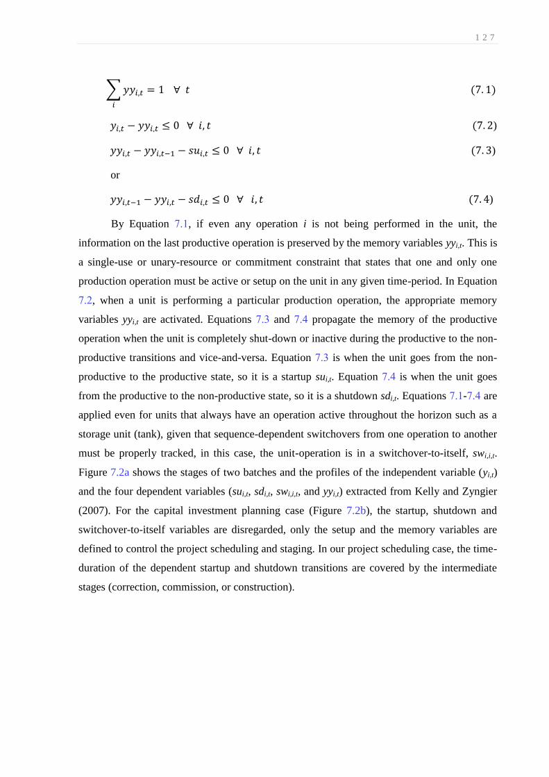
1 2 7

∑

( )

( )

( )

or

( )

By Equation 7.1, if even any operation i is not being performed in the unit, the

information on the last productive operation is preserved by the memory variables yyi,t. This is

a single-use or unary-resource or commitment constraint that states that one and only one

production operation must be active or setup on the unit in any given time-period. In Equation

7.2, when a unit is performing a particular production operation, the appropriate memory

variables yyi,t are activated. Equations 7.3 and 7.4 propagate the memory of the productive

operation when the unit is completely shut-down or inactive during the productive to the non-

productive transitions and vice-and-versa. Equation 7.3 is when the unit goes from the non-

productive to the productive state, so it is a startup sui,t. Equation 7.4 is when the unit goes

from the productive to the non-productive state, so it is a shutdown sdi,t. Equations 7.1-7.4 are

applied even for units that always have an operation active throughout the horizon such as a

storage unit (tank), given that sequence-dependent switchovers from one operation to another

must be properly tracked, in this case, the unit-operation is in a switchover-to-itself, swi,i,t.

Figure 7.2a shows the stages of two batches and the profiles of the independent variable (yi,t)

and the four dependent variables (sui,t, sdi,t, swi,i,t, and yyi,t) extracted from Kelly and Zyngier

(2007). For the capital investment planning case (Figure 7.2b), the startup, shutdown and

switchover-to-itself variables are disregarded, only the setup and the memory variables are

defined to control the project scheduling and staging. In our project scheduling case, the time-

duration of the dependent startup and shutdown transitions are covered by the intermediate

stages (correction, commission, or construction).

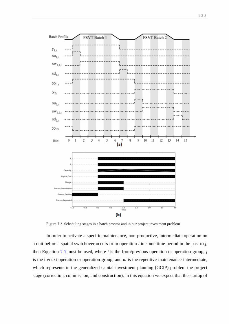
1 2 8

Figure 7.2. Scheduling stages in a batch process and in our project investment problem.

In order to activate a specific maintenance, non-productive, intermediate operation on

a unit before a spatial switchover occurs from operation i in some time-period in the past to j,

then Equation 7.5 must be used, where i is the from/previous operation or operation-group; j

is the to/next operation or operation-group, and m is the repetitive-maintenance-intermediate,

which represents in the generalized capital investment planning (GCIP) problem the project

stage (correction, commission, and construction). In this equation we expect that the startup of

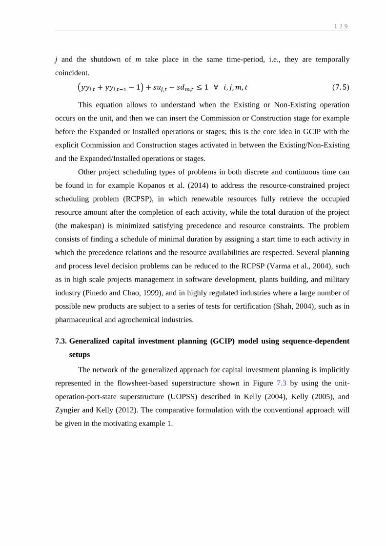
1 2 9

j and the shutdown of m take place in the same time-period, i.e., they are temporally

coincident.

( ) ( )

This equation allows to understand when the Existing or Non-Existing operation

occurs on the unit, and then we can insert the Commission or Construction stage for example

before the Expanded or Installed operations or stages; this is the core idea in GCIP with the

explicit Commission and Construction stages activated in between the Existing/Non-Existing

and the Expanded/Installed operations or stages.

Other project scheduling types of problems in both discrete and continuous time can

be found in for example Kopanos et al. (2014) to address the resource-constrained project

scheduling problem (RCPSP), in which renewable resources fully retrieve the occupied

resource amount after the completion of each activity, while the total duration of the project

(the makespan) is minimized satisfying precedence and resource constraints. The problem

consists of finding a schedule of minimal duration by assigning a start time to each activity in

which the precedence relations and the resource availabilities are respected. Several planning

and process level decision problems can be reduced to the RCPSP (Varma et al., 2004), such

as in high scale projects management in software development, plants building, and military

industry (Pinedo and Chao, 1999), and in highly regulated industries where a large number of

possible new products are subject to a series of tests for certification (Shah, 2004), such as in

pharmaceutical and agrochemical industries.

7.3. Generalized capital investment planning (GCIP) model using sequence-dependent

setups

The network of the generalized approach for capital investment planning is implicitly

represented in the flowsheet-based superstructure shown in Figure 7.3 by using the unit-

operation-port-state superstructure (UOPSS) described in Kelly (2004), Kelly (2005), and

Zyngier and Kelly (2012). The comparative formulation with the conventional approach will

be given in the motivating example 1.

1 3 0

Figure 7.3. Motivating example 1: small GCIP flowsheet for expansion.

In Figure 7.3, the diamond shapes or objects are the perimeter unit-operations where

they consume material A (source) and produce material B (sink), i.e., in- and out-bound

resources. We have just one process unit with three operations of Existing, Commission, and

Expanded as shown by the square boxes with an “x” through it indicating it is a continuous-

process type ( ). The first dotted line box highlights that only one unit-operation can be

active or setup at a time, i.e., a unary resource or the unit commitment constraint. The small

circles are the in-ports ( ) and out-ports ( ), where these ports have the attributed lower and

upper yields available similar to the modeling of generalized network-flow problems, i.e.,

having the previously mentioned Leontief input-output models with intensities, bill-of-

material, or transfer coefficients. The port-states allow flow into and out of a unit and can be

considered as flow-interfaces similar to ports on a computer, e.g., nozzles, spouts, spigots.

Port-states also provide an unambiguous description of the flowsheet or superstructure in

terms of specifically what type of materials or resources are being consumed and produced by

the unit-operation. Port-states can also represent utilities (steam, power), utensils (operators,

tools) as well as signals such as data, time, tasks, etc. In-ports and out-ports can be compared

to the mixers and splitters found in Moro and Pinto (1998) formulation, but including the

concept port-state, which is symmetric with unit-operation.

Each of the two perimeters, A and B, can have tanks available for storage, and is a

requirement when balancing the production-side and transportation-side supply and demand

of the value-chain. Finally, the lines or arcs between the unit-operations and port-states and

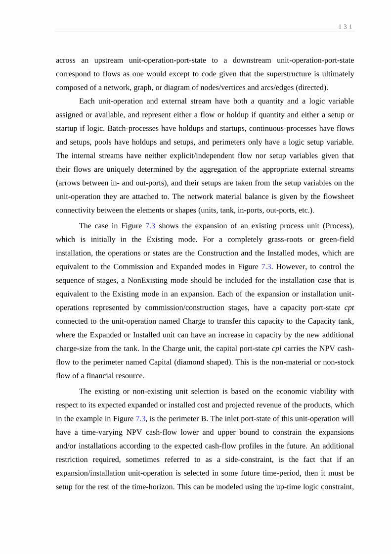
1 3 1

across an upstream unit-operation-port-state to a downstream unit-operation-port-state

correspond to flows as one would except to code given that the superstructure is ultimately

composed of a network, graph, or diagram of nodes/vertices and arcs/edges (directed).

Each unit-operation and external stream have both a quantity and a logic variable

assigned or available, and represent either a flow or holdup if quantity and either a setup or

startup if logic. Batch-processes have holdups and startups, continuous-processes have flows

and setups, pools have holdups and setups, and perimeters only have a logic setup variable.

The internal streams have neither explicit/independent flow nor setup variables given that

their flows are uniquely determined by the aggregation of the appropriate external streams

(arrows between in- and out-ports), and their setups are taken from the setup variables on the

unit-operation they are attached to. The network material balance is given by the flowsheet

connectivity between the elements or shapes (units, tank, in-ports, out-ports, etc.).

The case in Figure 7.3 shows the expansion of an existing process unit (Process),

which is initially in the Existing mode. For a completely grass-roots or green-field

installation, the operations or states are the Construction and the Installed modes, which are

equivalent to the Commission and Expanded modes in Figure 7.3. However, to control the

sequence of stages, a NonExisting mode should be included for the installation case that is

equivalent to the Existing mode in an expansion. Each of the expansion or installation unit-

operations represented by commission/construction stages, have a capacity port-state cpt

connected to the unit-operation named Charge to transfer this capacity to the Capacity tank,

where the Expanded or Installed unit can have an increase in capacity by the new additional

charge-size from the tank. In the Charge unit, the capital port-state cpl carries the NPV cash-

flow to the perimeter named Capital (diamond shaped). This is the non-material or non-stock

flow of a financial resource.

The existing or non-existing unit selection is based on the economic viability with

respect to its expected expanded or installed cost and projected revenue of the products, which

in the example in Figure 7.3, is the perimeter B. The inlet port-state of this unit-operation will

have a time-varying NPV cash-flow lower and upper bound to constrain the expansions

and/or installations according to the expected cash-flow profiles in the future. An additional

restriction required, sometimes referred to as a side-constraint, is the fact that if an

expansion/installation unit-operation is selected in some future time-period, then it must be

setup for the rest of the time-horizon. This can be modeled using the up-time logic constraint,

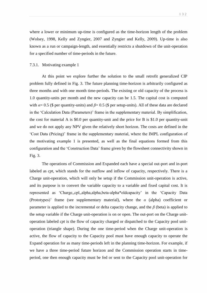
1 3 2

where a lower or minimum up-time is configured as the time-horizon length of the problem

(Wolsey, 1998, Kelly and Zyngier, 2007 and Zyngier and Kelly, 2009). Up-time is also

known as a run or campaign-length, and essentially restricts a shutdown of the unit-operation

for a specified number of time-periods in the future.

7.3.1. Motivating example 1

At this point we explore further the solution to the small retrofit generalized CIP

problem fully defined in Fig. 3. The future planning time-horizon is arbitrarily configured as

three months and with one month time-periods. The existing or old capacity of the process is

1.0 quantity-units per month and the new capacity can be 1.5. The capital cost is computed

with α= 0.5 ($ per quantity-units) and β= 0.5 ($ per setup-units). All of these data are declared

in the ‘Calculation Data (Parameters)’ frame in the supplementary material. By simplification,

the cost for material A is $0.0 per quantity-unit and the price for B is $1.0 per quantity-unit

and we do not apply any NPV given the relatively short horizon. The costs are defined in the

‘Cost Data (Pricing)’ frame in the supplementary material, where the IMPL configuration of

the motivating example 1 is presented, as well as the final equations formed from this

configuration and the ‘Construction Data’ frame given by the flowsheet connectivity shown in

Fig. 3.

The operations of Commission and Expanded each have a special out-port and in-port

labeled as cpt, which stands for the outflow and inflow of capacity, respectively. There is a

Charge unit-operation, which will only be setup if the Commission unit-operation is active,

and its purpose is to convert the variable capacity to a variable and fixed capital cost. It is

represented as ‘Charge,,cpl,,alpha,alpha,beta-alpha*oldcapacity’ in the ‘Capacity Data

(Prototypes)’ frame (see supplementary material), where the α (alpha) coefficient or

parameter is applied to the incremental or delta capacity change, and the β (beta) is applied to

the setup variable if the Charge unit-operation is on or open. The out-port on the Charge unit-

operation labeled cpt is the flow of capacity charged or dispatched to the Capacity pool unit-

operation (triangle shape). During the one time-period when the Charge unit-operation is

active, the flow of capacity to the Capacity pool must have enough capacity to operate the

Expand operation for as many time-periods left in the planning time-horizon. For example, if

we have a three time-period future horizon and the Commission operation starts in time-

period, one then enough capacity must be fed or sent to the Capacity pool unit-operation for

1 3 3

time-periods two and three (END). In this way, the capacity to be expanded or installed, an

extensive amount, is approximated as an intensive value. As example, for the first period, it is

represented as ‘Charge,,cpt,,1.0*(END-1.0),1.0*(END-1.0),,0.0,1.0’ in the ‘Command Data

(Future Provisos)’ frame (see supplementary material).

The cpt in-port on the Expanded operation will draw only up to the maximum

allowable or upper limit of the expanded capacity allowed from the Capacity pool, and this

will control the capacity charge-size, throughput, or flow through the unit-operation for the

Expanded operation. In order to do this, the lower yield bound on the cpt in-port is configured

as one and the upper yield bound as infinity or some large number. This will regulate the

capacity of the Expanded unit-operation as in ‘Process,Expanded,cpt,,1.0,large’ in the

‘Capacity Data (Prototypes)’ frame (see supplementary material).

The problem is solved using MILP with a provably optimal objective function of

$3.25. If we apply no expansion, then the profit would be $3.0 since the existing capacity is

1.0 for three time-periods. Since the profit is $0.25 more than $3.0, then there has been an

expansion where the Commission operation is setup or started in time-period one. To perform

an expansion of 1.5 – 1.0 = 0.5 quantity-units then, the capital cost required is 0.5 * 0.5 + 0.5

= $0.75. Given the timing of the Commission stage, this implies that the Expanded stage

occurs in time-periods two and three, which is enforced by the sequence-dependent setup

modeling, i.e., after the Commission stage only the Expanded stage can be setup for the rest

of the horizon. With an expansion capital cost of $0.75 and a revenue for the sale of material

B of 1.0 + 1.5 + 1.5 = $4.0 for the three planning periods, this leaves a profit of $4.0 - $0.75 =

$3.25, which is the same value found by the MILP. The Gantt chart for this example is found

in Figure 7.4. In this case, we are considering the Commission mode with the same capacity

as in the existing to permit production during this stage, since an interruption of this

production in the first time period can impede the expansion.

1 3 4

Figure 7.4. Gantt chart for expansion of a generalized CIP example.

From the Gantt chart in Figure 7.4 we can verify the timing for the Commission and

Expanded unit-operation on the Process unit. The interesting detail is the Capacity pool

holdup or inventory trend of capacity, which is shown as the grey line inside the black horizon

bar. We can see a charge of capacity in time-period one, and a continuous draw or dispatch

out in time-periods two and three. The black horizon bar means that the binary variable of the

shape is active.

7.3.2. Motivating example 2

An installation structure similar to the expansion in Figure 7.3 is added to the

motivating example 2. The Existing, Commission, and Expanded modes or stages in the

installation case is changed to NonExisting, Construction, and Installed modes as shown in

Figure 7.5.

1 3 5

Figure 7.5. Motivating example 2: small GCIP flowsheet for expansion and installation.

The problem is solved using MILP with a provably optimal objective function of

$5.00. If we apply no expansion or installation then the profit would be $3.0 since the existing

capacity is 1.0 for three time-periods. To perform an expansion, we have the same as the in

motivating example 1. To perform an installation of the same 1.5 quantity-units, the capital

cost required is 1.5 * 0.5 + 0.5 = $1.25. Given the timing of the Construction stage, this

implies that the Installed stage occurs in time-periods two and three which is enforced by the

sequence-dependent setup modeling, i.e., after the Construction stage only the Installed can be

setup for the rest of the horizon. Different from the expansion cost evaluation, there is no

existing capacity for an installation (NonExisting mode), so the alpha*oldcapacity is not

discounted in the beta cost. The production from the Construction stage was disregarded by

considering the out-port linked to the product perimeter B with zero yield. With an expansion

capital cost of $0.75 and an installation capital cost of $1.25, a revenue for the sale of material

1 3 6

B of 1.0 + 1.5 + 1.5 = $4.0 from the expanded existing unit and 0.0 + 1.5 + 1.5 = $3.0 from

the installed non-existing unit for the three planning periods. This leaves a profit of $4.0 +

$3.0 - $0.75 - $1.25 = $5.0, which is the same value found by the MILP. The Gantt chart for

this example is found in Figure 7.6. Also, the commission mode has the same capacity as in

the existing to permit production during this stage.

Figure 7.6. Gantt chart for expansion and installation of a generalized CIP example.

7.4. Examples

The capital investment planning examples presented in the following include (i) a

retrofit problem for process unit expansion and extension with fixed investment costs, as the

transformations are pre-defined as fixed values, and (ii) an expansion and installation problem

on an integrated oil-refinery with variable costs, since the size of the revamped (expanded or

installed) capacity can vary. The examples were modeled using Industrial Algorithm’s IMPL

and solved using IBM’s CPLEX 12.6.

7.4.1. Retrofit planning of a small process network

Our illustrative example is taken from Jackson & Grossmann (2002). There are 3 feeds

and 2 product materials (A,B,C,D,E) with 3 processes (Figure 7.7) that can be either expanded

(capacity increase) or extended (conversion increase) or both, considering fixed values as the

transformations. A total of three time periods is considered.

1 3 7

Figure 7.7. Retrofit example for capacity (expansion) and capability (extension) projects.

In Figure 7.8 is our new flowsheet representation with the Existing, Commission, and

Expanded (or Extended) stages shown explicitly where M denotes the flow of money

(investment costs). The associated MILP model using our approach in IMPL includes 403

constraints, 114 continuous variables, and 154 binary variables, and was solved with CPLEX

in less than 0.25-seconds to provably optimal. The convex hull MILP formulation proposed in

Jackson & Grossmann (2002) has 394 constraints, 244 continuous variables, and 36 discrete

variables. They also modeled the problem using conventional big-M constraints to

reformulate the GDP into an MILP more compact with 328 constraints, 124 continuous

variables, and 36 discrete variables.

1 3 8

Figure 7.8. UOPSS flowsheet for Jackson and Grossmann (2002) example.

The two Gantt charts shown in Figure 7.9 have the same solution with an NPV =

11.841 M$ over three one-year time-periods, where Process 1 has its capacity expanded,

Process 2 is unchanged, and Process 3 is conversion (capability) extended. The commission

throughputs and yields are considered the same as in the expanded or extended modes in order

to compare with the Jackson and Grossmann (2002) example, where the project staging is

disregarded.

The two Gantt Charts show the same solution with an NPV = 11.841 M$ over 3 one-year time-

periods where Process 1 is capacity expanded, Process 2 is unchanged and Process 3 is conversion

(capability) extended.

Money or Pecuniary

1 3 9

Figure 7.9. Gantt chart for Jackson and Grossmann (2002) example.

It should be noted that the results of the example are different than the ones reported in

Jackson and Grossmann (2002), since these authors reported incorrect numbers in their Figure

3, although their original GAMS file was correct and is in fact the one we have used in this

chapter in Figure 7.9.

7.4.2. Oil-refinery process design synthesis

The oil-refinery example in Figure 7.10 represents a complete plant with expansions

and installations permitted only for the crude and vacuum distillation units (CDU and VDU)

over three time periods. The capacity upper bound for the other units is considered a large

number to avoid bottlenecks. The commission/expanded and the construction/installed

structures or shapes for the CDU and VDU are not depicted. They are constructed similarly to

the motivating examples.

1 4 0

Figure 7.10. Oil-refinery example flowsheet.

The considered MILP model includes 722 constraints, 170 continuous variables, and

200 binary variables, and was solved with CPLEX in 0.5-seconds, and solved to optimality

yielding a NPV = 732.94 M$.

In Fig. 11, CDU and VDU labels represent the expansions and the CDU2 and VDU2

the installations. As we now consider the commission stage in the expansions with zero

production, the problem only set up installation projects (CDU2 and VDU2). The charges of

these projects occur together with the constructions as well as the capacity tank filling. After

the constructions, the capacity of the new installed modes is continuously maintained as

shown in Figure 7.11.

1 4 1

Figure 7.11. Gantt chart for the CDU and VDU installations.

7.5. Conclusion

In summary, we have proposed a generalized network-flow MILP model using setups

approach to model and solve a typical capital investment planning problem considering

intermediate stages between the existing state (existing unit or new unit) and the final state

after the repair, retrofit, or revamp (expansion, extension and installation) projects. We have

applied the concepts of sequence-dependent setups to manage the project scheduling by

considering phasing (from one state to another) and the project execution similar to the

maintenance or purging stage as normally found in scheduling sequence-dependent

changeover problems. A unique and novel way is used to formulate the CIP problem using

capacity/capability and capital as flows in a scheduling environment. The problems are

relatively easy to implement without having to explicitly code the sets, parameters, variables

and constraints required in algebraic modeling languages such as AIMMS, AMPL, GAMS,

LINGO, MPL, MOSEL, OPL, etc. Instead, the modeling platform IMPL allows the modeler

or user the ability to configure the problem using semantic variables such as flows, holdups,

yields and setups, startups, etc. which is more intuitive and natural. Finally, our generalized

CIP formulation can be straightforwardly applied to any CIP problem found in many process

industries including such specific applications as shale-gas well startup and ore mining and

extraction planning which require more scheduling details to be considered.

1 4 2

Chapter 8

8. Phenomenological Decomposition Heuristic for Production Synthesis of

Oil-Refinery Units

The processing of a raw material is a phenomenon that varies its quantity and quality

along a specific network and logics to transform it into final products. To capture the

production framework in a mathematical programming model, a full space formulation

integrating discrete design variables and quantity-quality relations gives rise to large scale

non-convex mixed-integer nonlinear models often difficult to solve. In order to overcome this

problem, we propose a phenomenological decomposition heuristic to solve separately in a

first stage the quantity and logic variables in a mixed-integer linear model, and in a second

stage the quantity and quality variables in a nonlinear programming formulation. By

considering different fuel demand scenarios, the problem becomes a two-stage stochastic

programming model, where nonlinear models for each demand scenario are iteratively

restricted by the process design results. Three examples demonstrate the tailor-made

decomposition scheme to construct the complex oil-refinery process design in a quantitative

manner.

8.1. Introduction

Production optimization relating quantity and quality variables in processing

(blending, reacting, and separating) constraints are sufficient to describe planning and

scheduling problems for a given process design, sequence of operation, selection of tasks, etc.

On the other hand, for full-designed mixed-integer models, in spite of being necessary,

quantity-quality relationships solely are insufficient, because these problems must also be able

to deal with discrete decisions such as investment setup, project scheduling, plant shutdown,

assignment, sequencing, etc. The combination of quantity, quality and logic variables in a

single model results in a mixed-integer nonlinear programming (MINLP) model that is non-

convex due to, at the very least, the bilinear terms associated with quantity times quality

variables, but also due to the either-or logic decisions. While significant advances have been

recently made in MINLP solution efficiency (Belotti et al., 2013), a robust commercial

software tool is still not available for solving non-convex MINLP industrial-sized problems.

1 4 3

Hence, alternative and heuristic methods are proposed in order to solve such large-scale

MINLP problems.

A decomposition solution method, denoted here as the phenomenological

decomposition heuristic (PDH), is proposed to avoid the full space MINLP model, which is

decomposed, partitioned, or separated into two simpler sub models namely logistics (quantity

and logic) and quality (quantity and quality) optimization sub problems. The logistics model

solves a problem with quantity and logic variables subject to quantity and logic balances and

constraints (Kelly and Mann, 2003; Kelly, 2004a; Kelly, 2006; Zyngier and Kelly, 2009).

Quality optimization solves for quantity and quality variables subject to quantity and quality

balances and constraints (Kelly, 2003; Kelly, 2004a; Kelly, 2004b) after the logic variables

have been fixed at the values obtained from the solution of the logistics optimization.

The proposed PDH methodology is applied to solve the strategic investment planning

problem in a two-stage stochastic programming model for different demand scenarios. The

goal is to maximize the net present value (NPV) to determine project setups and their related

new capacities by expansion and installation of units, which are scenario-independent in the

MILP master or high-level problem (first stage), so they are the linking variables over the

different scenarios. In this stage, fuel production, material flows, yields and other types of

variables for each scenario are modeled in a linear manner within the operational layer of the

MILP problem. The operational scenarios have the same discrete probability, so this value is

simply a coefficient in the scenarios’ operational amounts (gains and costs) taken into account

in the NPV objective function.

In the second stage, the NLP operational slave or lower-level problems are solved for

each scenario considering the process design found in the MILP problem, and new yields and

crude-oil diet compositions are updated in the next MILP iteration until both the MILP and

NLP solutions convergence on the objective function and variable solution values. The

combinatorial enumeration of projects within the MILP problem takes into account two

groups of binary constraints to reduce the tree search, the first considers investment decisions

in expansion and installation of process units and the second addresses process unit sequence-

dependency based on the possible connectivity in the oil-refinery framework, network, or

process design found among the worldwide sites included in this work.

This work is organized as follows. In section 8.2, the phenomenological

decomposition heuristic to construct the complex oil-refinery network is presented. Section

8.3 establishes the problem statement as well as the oil-refinery framework and groups of

1 4 4

units considered. The strategic investment problem is shown in section 8.4 with both the

conventional capital investment planning in an MILP formulation and the integer constraints

addressed in this work. Besides, the NLP formulation references for the operational layer

problem are presented in this section. In section 8.5, two examples are highlighted, the first is

a motivating example to better discuss the decomposition algorithm workflow using the

conventional and the generalized capital investment planning models (CCIP and GCIP)

without considering scenarios. The CCIP model is defined in this work and the GCIP model is

found in chapter 7. The second example uses the CCIP modeling for one oil-refinery site.

Conclusions and future work are presented in section 8.6.

8.2. Phenomenological decomposition heuristic

8.2.1. Partitioning (decomposition) and positioning of models

Partitioned or decomposed models demand more coding and calculation (Kallarath,

2011), and there is always a price or cost to be paid for their modularization with repeated

calculations, instead of solving the monolithic or full space problem directly (Conejo et al.,

2006). Partitioning is the notion of decomposing the problem into smaller sub problems along

its hierarchical (Kelly and Zyngier, 2008), structural or spatial (Kelly and Mann, 2004),

operational (Kelly, 2006), temporal (Kelly, 2002) and now phenomenological (Kelly, 2003,

Kelly and Mann, 2003, Kelly and Zyngier, 2015) dimensions. Positioning is the ability to

configure the lower and upper hard bounds and target soft bounds for any time-period over

the future time-horizon within the sub problem and is especially useful to fix variables (i.e.,

its lower and upper bounds are set equal), which will ultimately remove or exclude these

variables from the solver’s model or matrix.

Figure 8.1 highlights the partitioning along the phenomenological dimension of the

MINLP into two sub problems we call the quality and logistics sub problems as previously

mentioned, which is a rational break-down of the quantity, logic, and quality phenomena

(QLQP) or qualogistics and allows to iteratively and sequentially solve industrial-sized, -

scaled, and -scoped MINLP problems found in the process industries using what is considered

to be a natural and intuitive decomposition heuristic, strategy or algorithm.

1 4 5

Figure 8.1. Partitioning and positioning conjunction variables

The variables that connect, coordinate, match, transfer, or link, etc. one sub problem to

another are called the conjunction variables. Semantically the conjunction variables are

primarily intensive (do not scale with size as opposed to extensive variables which scale with

size) such as yields and setups/startups, although any QLQP variable can be a candidate such

as flows, holdups, switchovers, shutdowns, properties, and conditions. The proposed solution

procedure is relatively simple and first starts with a single or mono-period quality sub

problem (NLP) (partitioning) to generate starting or initial yields, which are then used as input

(positioning) to the multi-period logistics sub problem (MILP). Once an acceptably good

MILP solution is found then the values for the setup binary variables can be used to solve a

multiperiod quality sub problem and the solution process repeats between the two multiperiod

sub problems until a reasonable convergence between the NLP and MILP sub problem

objective functions (or other common variable) is found.

Similar to the depth-first with backtracking search found in Kelly (2002), this same

technique can also be employed here whereby each sub problem, due to its inherent non-

convexity, will most likely exhibit multiple local solutions. By retaining then recovering these

solutions using unformatted binary files for example and applying a systematic search

mechanism similar to branch-and-bound, multiple solution paths can be circumscribed where

the goal is to find the best overall or combined solution with the highest profit, best

performance and/or least amount of penalties, i.e., the combination of both MILP and NLP

sub problem solutions making up the MINLP problem.

In previous works, an MINLP crude-oil scheduling problem using priority-slot based

continuous-time formulation (Mouret et al., 2009) compares the full space solution and its

decomposed MILP-NLP problem by neglecting the pooling or blending nonlinear constraints

in the MILP model, and then re-composing the model in an NLP problem by relating quantity

and quality variables for the binary results found in the MILP model. In their work the full

space solution becomes intractable for industrial-sized examples, but they are solved in

MILP-NLP decomposition with an objective function gap between both solutions lower than

1 4 6

4%. Only a small example considering a low number of time slots is solved using the MINLP

formulation, which yields the same result found in the decomposed solution, but with higher

computational expense.

The proposed phenomenological decomposition heuristic resembles the well-studied

approach suggested in Benders decomposition where “complicating” variables (in this case,

binary) are fixed such that a simpler problem may be solved which are later freed again for

the next iteration (Geoffrion, 1972). A similar method has also been applied for a different

purpose, namely that of integrating decentralized decision-making systems through a

hierarchical decomposition heuristic (HDH) (Kelly and Zyngier, 2008). In the context of the

integration between logistics and quality problems, the coordinator (logistics MILP sub

problem) would send what we call “logic pole-offers” to the cooperator (quality NLP sub

problem), which in turn would send back logic pole-offsets to the coordinator. This procedure

continues until convergence is achieved, hopefully providing at least a globally feasible

MINLP solution.

Other decomposition approaches include bi-level (Iyer and Grossmann, 1998) and

Lagrangean decomposition (Karuppiah and Grossmann, 2008). Similar to Benders

decomposition, the bi-level approach is based on the idea that some complicating variables

e.g., investment decisions or assignment variables, are withdrawn to solve an easier sub model

and then included in a further step fixing some results from the previous model. In their NPV-

based capital investment planning example with two sets of binary variables (selection and

expansion of process unit), the design master problem does not contain binary variables

associated with capacity expansion decisions. It only contains binary variables representing

the selection of a process over the entire planning horizon, so the high-level or design

problem is combinatorially less complex and selects a subset of processes for design.

Following the algorithm, the lower level planning problem is solved for the selected set of

processes to define the capacity expansion. Bounding information is used over the algorithm

based on specific relaxations that under and overestimate the investment costs in the NPV

maximization.

On the other hand, in the Lagrangean decomposition a set of hard constraints is

violated by addition of a penalty term into the objective function to form an easier problem,

the dual problem, although it may require excessive computation for even small problems by

the additional Lagrangean multipliers determination usually through subgradient optimization.

Large-scale process industry problems including multi-entity relationship by integrating the

1 4 7

production and distribution supply chain problems (You et al., 2011; Corsano et al., 2014)

showed that the bi-level decomposition (Iyer and Grossmann, 1998) requires smaller

computational times leading to solutions that are much closer to the global optimum when

compared to the full space solution and to Lagrangean decomposition (Guignard and Kim,

1987).

8.2.2. PDH algorithm for oil-refinery design synthesis

The proposed two-stage stochastic program scheme (Birge and Louveaux, 2011) displayed in

Figure 8.2 where the investment decisions are the first-stage variables (here-and-now)

considering scenario probabilities in a logistics (logic and quantity) problem and all

operational decisions modeling the necessary quantity and quality balances (quality problem)

are the second-stage decisions (wait-and-see) according to the demand realizations of the

scenarios. Considering the proposed modeling, the second-stage variables do not contain

discrete decisions related to the modes of operation and associated sequencing, transitions or

other logic relation, which would make the resulting two-stage stochastic programming

problem hard to solve.

Figure 8.2. Two-stage stochastic programming strategy.

The applied PDH algorithm flowchart is presented in Figure 8.3. Before to perform the

first stage problem, one quality optimization finds continuous variables x initial-values for all

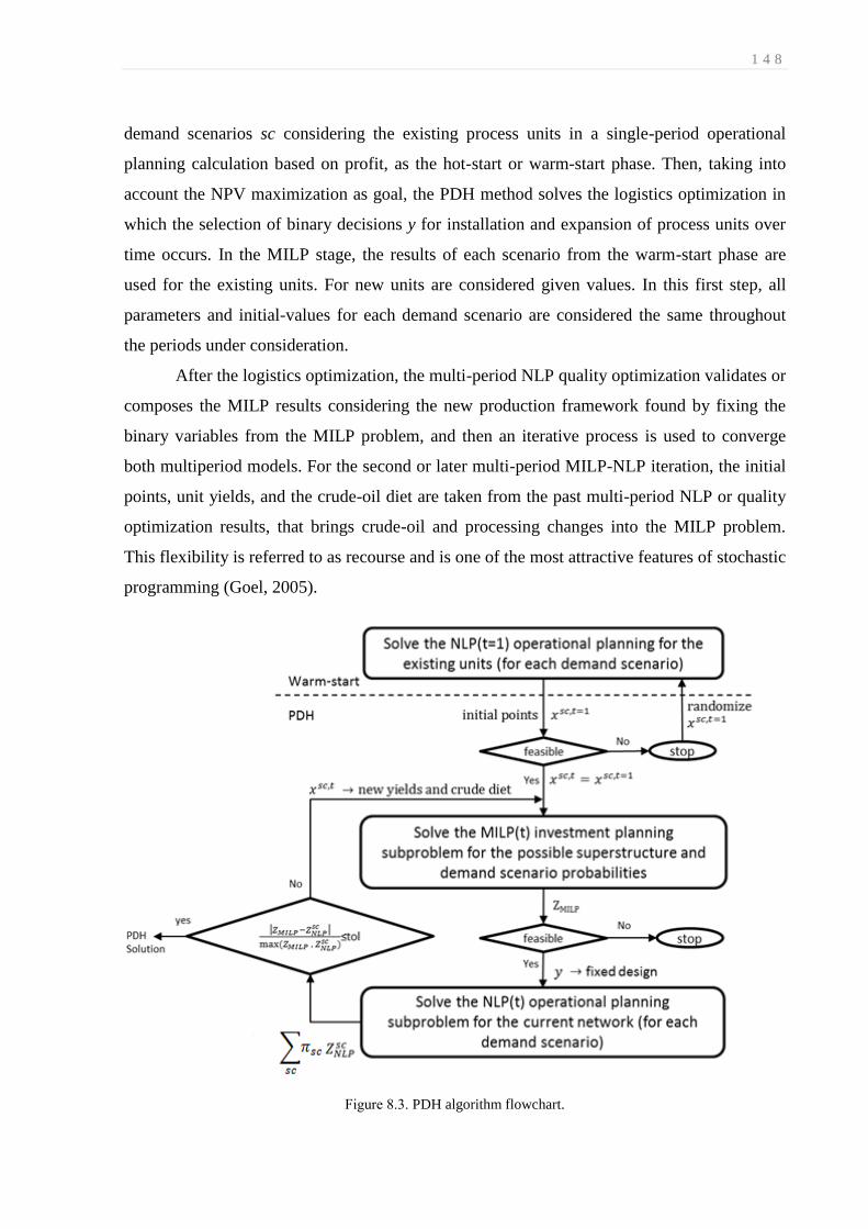
1 4 8

demand scenarios sc considering the existing process units in a single-period operational

planning calculation based on profit, as the hot-start or warm-start phase. Then, taking into

account the NPV maximization as goal, the PDH method solves the logistics optimization in

which the selection of binary decisions y for installation and expansion of process units over

time occurs. In the MILP stage, the results of each scenario from the warm-start phase are

used for the existing units. For new units are considered given values. In this first step, all

parameters and initial-values for each demand scenario are considered the same throughout

the periods under consideration.

After the logistics optimization, the multi-period NLP quality optimization validates or

composes the MILP results considering the new production framework found by fixing the

binary variables from the MILP problem, and then an iterative process is used to converge

both multiperiod models. For the second or later multi-period MILP-NLP iteration, the initial

points, unit yields, and the crude-oil diet are taken from the past multi-period NLP or quality

optimization results, that brings crude-oil and processing changes into the MILP problem.

This flexibility is referred to as recourse and is one of the most attractive features of stochastic

programming (Goel, 2005).

Figure 8.3. PDH algorithm flowchart.

1 4 9

Although the MILP sub problem uses a global search technique (branch-and-bound) to

find its best or globally optimal solution, the NLP sub problem does not, unless it is a global

nonlinear optimizer itself. Given that most, if not all, of industrial optimization problems are

non-convex, one simple solution would be to re-run the NLP using multiple randomized re-

starts for example and then to choose the best solution from this set of runs before proceeding

again to the MILP sub solver. This could help to improve the solution quality of the heuristic

in a straightforward manner.

When compared with the MINLP solutions, we should note that one of the advantages

of the PDH is that each sub problem is individually exposed in the algorithm, i.e., we solve

separate single-period NLP (like a root-relaxation), and the multi-period MILP and NLP

models iteratively. For industrial models, solving each sub problem individually provides a

useful intelligent problem-solving approach given that in MINLP solvers such as DICOPT, if

the root, MILP or NLP fails (infeasible, unconverted) there is no easy way to dissect and

diagnose it to locate the defects, faults, inconsistencies, etc. The PDH method decomposes

MINLP models into a logistics optimization or quantity-logic (QL) MILP master or high-level

problem and in a quality optimization or quantity-quality (QQ) NLP slave or lower-level

problem. Both sub problems are completely and independently solved and then their results

are used to integrate each other.

8.3. Problem Statement

The specific problem addressed in this paper can be stated as follows. Given future

demand scenarios sc, the decomposed MINLP based on our phenomenological decomposition

heuristic consists of determining the expansion of existing units and installation of new units

in petroleum refineries. The expansions and installations have investments costs defined by

varying and fixed terms. The parameter u represents the investment varying cost related to

the size of the unit u and u for the fixed cost related of the decision to invest or not in its

capacity at a certain time, which is the binary selection or investment setup. More details

about the investment cost curves and coefficients determination can be found in Appendix 0B.

These investment costs can take into account certain rules as depreciation, salvage value,

working capital or any governmental, environmental and/or company specific expenditures. A

review on the NPV investment cost or coefficient evaluation for oil-refinery units can be

1 5 0

found in Appendix0D and the investment costs per type of oil-refinery unit considered in this

work can be found in Table 4.1

The problem’s time horizon comprises investment t and operational t0 time periods as

seen in Figure 8.4, although the problem is only performed over each time-period t. The

shorter time-period t0 is only shown to understand how the MILP and NLP objective

functions are formulated. The operational layer in both linear and nonlinear formulation, the

former in the MILP problem and the latter in the NLP sub problems, calculates the annual

profit based on daily operations. After projects execution over each t, the new production

framework is considered within the following time periods to determine a new operational

profit that counts within the following periods.

Figure 8.4. Investment t and operational t0 time-periods.

The model considers unchangeable the operational variables within the investment time t,

although the operational cash inflows CFop(x,sc,t0) for each scenario with probability πsc vary

annually (over t0) by price increase. These annual operational gains are brought back to the

initial time ti (ti1, ti2,…; see Figure 8.4) after every each t0 using constant interest rate ir to

reflect the correction suffered by the future gains when it is considered at the present as

shown in Equation 8.1. The investment cash outflows CFin(x,y,t) are withdrawn at the

beginning of the time-period t with investment under consideration for expansion and

installation of the new capacities over time taking into account the framework superstructure,

given by the possible projects. The objective function calculation evaluates the potential gains

from the operational activities within the following time periods to decide whether the

discrete decisions to approve the projects at the beginning of each investment period are

1 5 1

made. As we consider that the project execution occurs within the time interval T with

several years, the investment is only allowed until the next-to-last time period (t < tend).

∑( ∑ (∑ ( )

( )

)

( )

( ) )

( )

A particular NPV formula for investment in oil-refineries is shown in chapter 4 to find

the required expansion in oil-refinery capacity for the future oil products market in Brazil.

The details about the deflationary NPV discounts are given in Appendix0D.

Within the NLP operational sub problems, the objective function of each scenario sc is

given by Equation 8.2. The investment costs ( ) are considered constant by fixing

the setups (projects approved) and their new capacities. For non-approved projects, their

constraints and variables are eliminated from the possible framework superstructure within

the NLP operational problems (second stage), and they are again included when the solution

returns to the MILP investment problem iteration (first stage) (see in Figure 8.3 to understand

the solution workflow).

∑( ∑ (

( )

( ) )

( )

( ) )

( )

Two examples are shown to demonstrate the tailored decomposition scheme:

1-) a motivating example to better access the decomposition algorithm workflow considering

expansion and installation of hydrotreating units using both the conventional and the

generalized capital investment planning models (CCIP and GCIP) without considering

demand scenarios. The CCIP model is defined in the following section and the GCIP model is

found in chapter 7.

2-) two industrial examples using the CCIP modeling considering one and four oil-refinery

sites with demand scenarios.

To formulate the multisite industrial-sized problem, the possible superstructure of

projects for investing must be known a priori to control models’ elements (equations,

variables, etc.) formation throughout the PDH algorithm, where is considered the network in

Figure 8.5 and the groups of units in Table 8.1. To generate the binary variables and their

1 5 2

linked variables along the PDH algorithm workflow, we consider at most four units u of the

same type within one refinery site.

Figure 8.5. Oil-refinery processing network example.

Table 8.1. Groups of units to build the superstructure.

Group Type Unit Name

Crude-oil consumer Crude-oil distillation CDU Crude-oil distillation unit

ATR consumer reduced crude distillation VDU vacuum distillation unit

catalytic cracking RFCC residue fluid catalytic cracking

VGO consumer catalytic cracking FCC fluid catalytic cracking

catalytic hydrocracking MHC medium hydrocracking

catalytic hydrocracking HCC hydrocracking

FK

FLD

ATR

CDU

SW2

VR

VDU

N

K

LD

HD

LCO

DO

HTD

HTK

FCC

D1HT

KHT

CLN

CHN

CLGO

CHGO

CMGO

D2HT

DC

REF

LCNHT

CLNHT

PQN

C1C2

HCN

LCN

C1C2

FN

FHD

GLN

(GLNC)

MSD

JET

LSD

HTCLN

HTLCN

FO

REFOR

C1C2 FG

LPG

LVGO

HVGO

00

ASPR

DAO

PDA

RFCC

SW3

SW1

HCCO

Crude

HCCD

HCCK

HCCN

HCC

UHSD

COKE

H2

COKE

LSDimp

GLNimp

(GLNA)

ETH

JETimp

LPGimp

ST

GOST

LNST

HNST

FK, FLD

HSD

C3C4

C3C4

C1C2

C3C4

DEBUT

SUPER

C3C3=

C4C4=

C3=

C3

C4C4=

C1C2

C3C4

1 5 3

VR consumer Extraction PDA propane/butane deasphalting

delayed thermal cracking DCU delayed coker unit

thermal cracking TCU thermal cracking unit

Hydrotreater (HT) Hydrotreating LCNHT light cracked naphtha HT

Hydrotreating CLNHT coker light naphtha HT

Hydrotreating KHT kerosene HT

Hydrotreating DHT diesel HT

Octane booster chain cycling REF reformer

chain isomerization ISO isomerization

C3 to C5 combination ALK alkylation

Fractionator C3 and C4 distillation DEBUT debutanizer

C3 and C3= distillation SUPER superfractionator (C3 + C3=)

naphtha separation ST stabilizer

In the PDH model, the three optimization areas within the oil-refinery boundaries are

integrated. The first is the crude-oil diet determination using the improved swing-cut

modeling considering pseudocomponents, hypotheticals, or micro-cuts distribution as in

chapter 5. The second area of optimization covers oil-refinery unit processing transformations

to vary quantity and quality variables in hydrotreaters, fluid catalytic cracking units (FCC and

RFCC), and propane desasphalting. In the third area, intermediate and final blends are

optimized considering quality specifications.

Within the MILP design problem, the aforementioned oil-refinery optimization areas

are adapted to avoid nonlinearities. The distillate streams only include yield determination

given by Equations 5.1-5.3 in improved swing-cut modeling addressed in chapter 5. The

processing transformations are linear considering input-output yield models, conversions or

rates given by the last nonlinear iteration. And the blending correlations are neglected or

linear related by fixing the qualities from the last nonlinear iteration.

8.4. Process design synthesis of multisite refineries formulation

In each processing center or refinery r, the investment layer problem controls the

capacity QCr,u,n,t of each nth-unit u,n over the investment time t. Only for the selected

1 5 4

investments (yr,u,n,t = 1) are the installations QIr,u,n,t and expansions QEr,u,n,t allowed. At each t,

the unit throughput QFr,u,n,sc,t, regardless of the demand scenario sc, cannot exceed the unit

capacity as shown in Equation 8.3. Only in the following period the unit capacities under

expansion or installation are started up after their project execution within T.

(8.3)

8.4.1. MILP investment planning model

Moro et al. (1998), Pinto et al. (2000) and Neiro and Pinto (2004) modeled operational

planning and scheduling cases for oil-refinery units considering a network whose streams are

linked to them by mixers and splitters as shown in Figure 8.6. The scenario index sc was

omitted for the sake of simplicity.

Figure 8.6. Material balance in u.

Equation 8.4 represents the mixer concentrating upstream streams up, and Equation

8.5 represents the splitter distributing downstream streams do.

∑

( )

( )

∑

( )

( )

Product yields of the units can be considered fixed values, as in the MILP problem, or

they can vary throughout the processing network, as in the NLP sub problems for some units,

and in this case a nonlinear constraint is formed by the quantity-quality variation. These yields

Yr,u,n,s,sc,t are given as a unit throughput ratio for each stream s, as seen in Equation 8.6. In the

MILP problem, they are generated by the previous NLP problems either in the warm-start or

1 5 5

in last multiperiod NLP operational planning sub problem solved. For the new units or

installations, the unit yields are given in the first MILP step. Distillate yields can vary in the

MILP problem in a linear formulation by using the swing-cut methodology in chapter 5.

( )

The unit capacities within an oil-refinery r can be updated after the project execution

to expand existing or install new assets. The capacity expansion QEr,u,n,t and installation QIr,u,n,t

of a unit in a certain time (t < tend) are active by the constrains 8.7 and 8.8. When an oil-

refinery process unit is revamped, the reasonable minimum capacity expansion is around 10%

of its current capacity. The maximum reaches around 30% depending on the unit equipment

complexity. For higher capacity requirements a new unit is installed.

( ) (8.7)

( ) (8.8)

In the first investment time period, the operational gains derive from the existing units

and their initial capacities are given by EXCAPr,u,n,t=1. After the project execution intervals, a

new capacity can be added to the unit and another profit is found in the operational layer for

the following investment time period if the project is approved, as shown in Equations 8.9 and

8.10.

( ) (8.9)

( ) (8.10)

With respect to the capital amount available in each investment time t, the liquid cash

expenses to build the units is lower than the limit capital for investment LCIt as seen in

Equation 8.11.

∑ (

)

( )

∑ (

)

( )

( )

1 5 6

8.4.2. Integer constraints for investment

Equations 8.12-8.15 are introduced to control the investment logic. Equations 8.12 and

8.13 permit the expansion (ye) and installation (yi) occurrence of a specific unit u only once

over all time periods with investment under consideration (t < tend). Some refining units such

as CDU can have more than one expansion and its life-time, but in this work all units have

only one. Equations 8.12 and 8.13 must be active over all periods with investment under

consideration to maintain the MILP investment planning approach functionality as defined in

this work.

∑

( )

∑

( )

The integer constraints defined in Equations 8.14-8.19 can be added or excluded in the

MILP solution. The first group, Equations 8.14 and 8.15, is related to investment logic when

expansion of existing units and installation of new ones are being modeled. Equation 8.14

allows only one investment (expansion or installation) per type of unit to avoid investing in

more than one unit of the same type at the same time. Equation 8.15 is similar to Equation

8.14, excepting that the types of unit are arranged by groups considering their functionality,

like those units responsible for the octane number boosting such as reformer (REF), alkylation

(ALK) and isomerization (ISO) or unit consuming the same type of feed such as vacuum

distillation unit (VDU) and residuum fluid catalytic cracking (RFCC), both atmospheric

residuum consumers (ATRC). Again, both Equations 8.14 and 8.15 can be withdrawn from

the model once they only reduce the binary search tree to prevent different project for the

same process needs. It is preferred to invest in one larger process unit than two or three small

ones.

∑( )

( )

∑∑( )

( )

1 5 7

8.4.3. Integer constraints for framework sequence-dependency

The second group of binary constraints, Equations 8.16-8.19, is related to the oil-

refinery processing framework precedency. It means that sequence-dependency logic exists to

invest in a certain type of unit if another investment is set up. The proposed disjunction to

manage the quantity transformations throughout the oil-refinery network is given in QTD,

where y means investment in projects by expansion or installation of capacity. The indices for

refinery r, number of unit n, and time t were excluded from QTD for the sake of simplicity.

GOC and VRC are gasoil and vacuum residue consumers, respectively.

[

[

] [

]

]

[

] ( )

In refineries with high production of fuel oil streams (≥ 15% of the CDU feed), the

investment in VRC unit can be a profitable choice since it converts low value streams to light

and medium products such as gasoline and diesel and requires less investment in downstream

units when compared with CDU investments. In high fuel oil production, the first disjunction

(yCDU yCDU) in Equation 8.16 is true, meaning CDU or no CDU, and decides about the oil-

refinery production growth by considering capacity increase in (i) crude distillation unit

(CDU) by feeding the whole refinery with higher throughputs or in (ii) VRC units such as

delayed coker unit (DC), propane deasphalting (PDA), and thermal cracking unit (TC), that is

the no CDU condition.

( )

∑( ) ∑ ∑( )

( )

The disjunction in the second level (yVDU yVDU) decide about the consumption of

the atmospheric residue (ATR) formed by the CDU investment, so it implies in yCDU yVDU

yVDU. In the common oil-refinery network, ATR is the VDU feed, where vacuum gasoil

(VGO) and vacuum residue (VR) are produced. If the VDU unit is not invested (yVDU), the

alternative is to increase the capacity of ART consumer units (ATRC) such as RFCC.

Equation 8.17 represents the second disjunction with the previous implication of the CDU

1 5 8

investment due to the consequent increase in ATR. As seen, only one type of project to

consume ATR within the refinery r in each time t is permitted, if the CDU investment occurs.

The possibilities are expansion or installation of VDU or other ATRC units.

( )

∑( ) ∑ ∑( )

∑[( )]

( )

A straightforward VDU investment consequence is the implication of capacity

addition of vacuum gasoil and residue consumer units (GOC and VRC) to convert the VDU

streams (GO and VR) into light and medium streams. The main GOC units are fluid catalytic

cracking (FCC) and medium and high severity hydrocracking (MHC and HCC). The VRC

units are DC and TC by thermal cracking or PDA by solvent extraction. Equation 8.18

represents the yVDU yGOC implication and Equation 8.19 the yVDU yVRC.

∑ ∑( )

∑[( )]

( )

∑ ∑( )

∑[( )]

( )

Other sequence-dependent logic to complete the oil-refinery network are disregarded

because gas, light, or medium streams formed by CDU, ATRC, GOC, and VRC units can be

dispatched to several downstream units such as fractionators, hydrotreaters, reformers, etc.,

that can have some idling capacity, so the new amounts of the intermediate streams formed by

the units addressed in the quantity disjunction QTD will determine the capacity needs for their

downstream units.

8.4.4. NLP operational planning model

The processing nonlinearities are related to the CDU/VDU, PDA, FCC, and

hydrotreater (HT) outputs. For CDU/VDU is considered the improved swing-cut modeling

(chapter 5) to calculate the quantity and quality variations (yields and properties) of the

1 5 9

distillate streams. The crude-oil diet or basket are found considering this improved swing-cut

NLP model by treating the crude as micro-cuts, psedocomponents, or hypotheticals pieces of

hydrocarbon material discretized within 10ºC, from pentane to heavy fractions up to 850ºC.

The FCC is configured with the delta-based model from Moro et al. (1998) to predict yields

variation based on Conradson carbon residue in feed and reactor and feed temperature

deviation. The PDA modeling simply considers the operational variable extraction factor as

the de-asphalted oil yield. The HT main transformation is the sulfur concentration reduction,

but the consequent specific gravity and octane number reductions are also regarded. All

streams with fixed yields and properties are given in the supporting information.

All blending equations are given in chapter 3. The properties being considered are the

volume-based (specific gravity, olefin, and aromatic content), the mass-based (sulfur content,

acidity, and Conradson carbon residue) and the ad-hoc octane number (research octane

number, and motor octane number).

8.5. Results and discussion

8.5.1. Motivating example

The motivating example is solved using the conventional and the generalized capital

investment planning (CCIP and GCIP) formulations without considering NPV deflation and

uncertainties from scenarios. The CCIP model is developed in GAMS (Brooke et al., 1992)

and the GCIP in IMPL. In the example depicted in Figure 8.7, the hydrotreater DHT1

produces 50 wppm sulfur diesel (D50) from a source containing 1000 wppm of sulfur

(D1000), wppm is ppm in weight basis. As the severity of the DHT1 varies between 0.90 and

0.95, the unit is not able to reduce the sulfur content to 15 wppm S (D15) as required in a

future scenario, so a new hydrotreater with higher severity must be installed. The severity of

the new unit DHT2 is between 0.90 and 0.99 and there is no explicit consumption of

hydrogen shown given that it is not perceived as a bottleneck or active constraint.

1 6 0

Figure 8.7. Initial and final network for 50 and 15 wwpm S diesel.

This is an MINLP problem given that all flows are variable as well as the specific

gravities and sulfur contents including the severity times sulfur thus resulting in bi-linear and

tri-linear terms with plus and minus coefficients making the NLP quality sub problem non-

convex. Due to the setup logic variables for the expansion and/or installation logic decisions

we have the integer or discrete (binary) variables resulting in the MINLP and more

appropriately a non-convex MINLP problem.

In the hydrotreating process, there is a trade-off between the sulfur content reduction

and the amount of hydrotreated stream lost as naphtha, which is inevitably produced by

cracking side reactions in the carbon chain. The H2S formed by the sulfur removing at high

pressure of H2 and high temperature are recovered in a fractionation tower after the reactor

bed and its upper stream is known as wild naphtha, a mix of naphtha and H2S. The correlation

considered to calculate the yields for o and wn, respectively, the hydrotreated stream and the

wild naphtha, are o = (1 – (sev-0.90)/2) and wn = (sev-0.90)/2. In the severity lower bound

scenario (sev=0.90), the wn formation is zero in both hydrotreaters. In the severity upper

bound (sev = 0.95 for DHT1 and sev = 0.99 for DHT2) the wn formation is 2.5% for DHT1

and 4.5% for DHT2.

To give more degrees of freedom to the motivating example, the DHT2 output o can

flow to D50 and D15 sinks of diesel on-specification. Considering the proposed PDH

algorithm the sequence of problems to be solved is 1-) the single-period NLP problem to

generate optimal initial values and unit yields (warm-start), 2-) the multiperiod MILP model

to find the new process design by expansion and installation of unit, and 3-) the multiperiod

NLP model to find new yields considering the new process design. In the multiperiod models,

1 6 1

there are three periods considered and the iteration between the steps 3 to 2 is performed

while the multiperiod MILP and NLP objective functions are within a 1% relative gap. The

warm-start can be neglected by using given numbers for initial values and upper and lower

bounds in the MILP problem.

The density is required to perform the mass-basis sulfur balances, although we

considered it a fixed number without any changing in the process. There is no cost applied to

the supply of diesel nor is there a price for wild naphtha. However, the D50 product has a

price of 1.0 and the price for D15 is 1.2, which implies that it is more economical to produce a

lower sulfur diesel material especially when there is no raw material or operating costs

currently modeled, although there is loss of diesel to wild naphtha with the severity increase.

In the design problem, the initial capacity of the DHT1 is 1.0 and the expansion is permitted

at most at 50% of the existing capacity. For the installed DHT2, the maximum capacity is 1.5.

The variable and fixed costs of the installation are equal 0.5 $/volume and 0.5 $ respectively.

The expansion is 60% of the installation costs. The initial value of the DHT2 considers zero

formation of wild naphtha, meaning that if the severity of the new hydrotreater has been

modeled in the MILP, it would be considered 0.90, without loss of hydrotreated stream o to

wn. In this case, the DHT2 would not be able to produce diesel with 15 wppm of sulfur if it

was taken into account in the MILP problem.

CCIP modeling results 8.5.1.1.

Using the conventional capital investment planning (CCIP) formulation as defined in

this work, equations 8.12 and 8.13 are needed to avoid more than one investment in the same

unit. The results of the 3 steps are shown in Table 8.2. The problem is performed in the

GAMS modeling language, version 23.9.3, on an Intel Core 2 Duo (3.00 GHz, 16.0 GB of

RAM). As we can see, both expansion of DHT1 at 1.5 and installation of 1.5 of DHT2

occurred.

In the first MILP iteration, the objective function resulted in 5.800 $. When the new

process design scenario is used in the first iteration of the multiperiod NLP problem, with

DHT1 capacity expanded from 1 to 1.5 and DHT2 installed with 1.5 of capacity, the DHT2

produces diesel at 15 wppm and its severity resulted in 0.985 to avoid more less of DHT2

output as wn. The MILP and NLP problems in the second iteration have the same yields as in

the NLP(ite=1) as seen in Table 8.3, converging both problems to the same results. The NLP

1 6 2

solvers used is CONOPT, IPOPT and SNOPT, which converged in less than 0.01 seconds in

all cases, and the MILP solver is CPLEX with less than 0.01 seconds of solution.

Table 8.2. Motivating example results of the warm-start and the first PDH iteration

Table 8.3. Motivating example results for the second PDH iteration.

GCIP modeling results 8.5.1.2.

Figure 8.8 shows the unit-operation-port-state superstructure (UOPSS) or flowsheet

using the generalized capital investment planning (GCIP) modeling (chapter 7) where the

UOPSS shapes can be found in Kelly (2004), Kelly (2005), Zyngier and Kelly (2009), and

Zyngier and Kelly (2012). This problem is formulated whereby both the capacity and capital

cost for the expansion and installation of the diesel hydrotreating units (DHT1 and DHT2

respectively) are modeled as flows in a scheduling environment with project staging.

Diamond shapes are perimeters which indicate where material or even money and other

necessary resources can flow into or out of the problem. The square shapes with an “x”

through them are continuous-processes and the triangle shapes are pools or inventory/storage

NLP(t=1)

objective function 0.975

t1 t2 t3 t1 t2 t3

yield DHT1.o 0.9750 0.9750 0.9750 0.9750 0.9750 0.9750 0.9750

DHT1.wn 0.0250 0.0250 0.0250 0.0250 0.0250 0.0250 0.0250

DHT2.o 1.0000 1.0000 0.9575 0.9575

DHT2.wn 0.0000 0.0000 0.0425 0.0425

capacity DHT1 1.0 1.0 1.5 1.5 1.0 1.5 1.5

DHT2 1.5 1.5 1.5 1.5

severity DHT1 0.950 0.950 0.950 0.950

DHT2 0.985 0.985

MILP(ite=1) NLP(ite=1)

5.800 5.647

objective function

t1 t2 t3 t1 t2 t3

yield DHT1.o 0.9750 0.9750 0.9750 0.9750 0.9750 0.9750

DHT1.wn 0.0250 0.0250 0.0250 0.0250 0.0250 0.0250

DHT2.o 0.9575 0.9575 0.9575 0.9575

DHT2.wn 0.0425 0.0425 0.0425 0.0425

capacity DHT1 1.0 1.5 1.5 1.0 1.5 1.5

DHT2 1.5 1.5 1.5 1.5

severity DHT1 0.950 0.950 0.950

DHT2 0.985 0.985

MILP(ite=2) NLP(ite=2)

5.647 5.647

1 6 3

unit-operations. The circles are ports where an “x” inside is an out-port and without an “x” is

in-port and the lines connected to ports and units are what we call “internal streams”. Lines

with arrow-heads connecting out-ports to in-ports are called “external streams” and these

along with the unit-operations have setup and startup logic variables created as well as

switchovers and shutdown logic variables if up-times and/or down-times are configured to

manage the temporal transitions (Kelly and Zyngier, 2007 and Zyngier and Kelly, 2009).

Figure 8.8. Partitioning and positioning GCIP example UOPSS flowsheet.

The scope of this problem is to decide if the existing unit DHT1 should be expanded

via the commission-stage operation or not and to decide if the non-existing unit DHT2 should

be installed via the construction-stage operation or not. If so then there is a capital cost during

the commission and construction-stages for the capacity expansion and installation using a

variable and fixed cost linear expression of capital cost = alpha * (capacity_new –

capacity_old) + beta * setup, where if an installation, the old capacity is of course 0 (zero). A

more detailed description of this modeling can be found in chapter 7.

1 6 4

When we solve the NLP(t=1) (temporal relaxation) sub problem using SLPQPE, with

either CPLEX, COINMP, GLPK, or LPSOLVE as the LP solvers, we get an objective

function value of 0.975 currency-units given that we have only allowed the existing DHT1

and non-existing DHT2 unit-operations to be active during the mono-period time-horizon in

order to provide starting, initial, or default yields to the multiperiod MILP, i.e., no capital

costs incurred. The 0.975 value corresponds to the fact that only flow from the

DHT1,Existing,o out-port to the D50,i in-port is active in the amount of 0.975 flow-units.

Upon solving the multiperiod MILP using CPLEX, COINMP, GLPK, or LPSOLVE we get

an objective function value of 5.800 currency-units which corresponds to the profit of

performing the DHT1 commission-stage in time-period 1 and DHT2 construction-stage also

in time-period 1. This allows two time-periods for expanded capacity for DHT1 and also two

time-periods for newly installed and extended capacity and capability for DHT2, i.e., the

DHT2 unit can produce both D50 and D15 due to its extended conversion. The Gantt chart in

Figure 8.9 displays the setup logic variables in black horizontal bars for all unit-operations.

Figure 8.9. Gantt Chart with 1-period and 3-period Past and Future Horizons for the multiperiod MILP.

Using the fixed setups from the multiperiod MILP for both the unit-operations and the

unit-operation-port-state to unit-operation-port-state external streams, we get a profit of 5.647

currency-units from the multiperiod NLP sub problem solution. Solving again the MILP with

the new fixed/finite yields from the NLP we converge on an objective function value of 5.647,

that is the same result found in the CCIP example. In this GCIP model, the production in the

commission phase for the expansion is considered the same as its existing mode in order to

compare both CCIP and GCIP results.

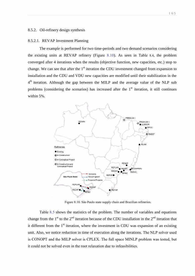
1 6 5

8.5.2. Oil-refinery design synthesis

REVAP Investment Planning 8.5.2.1.

The example is performed for two time-periods and two demand scenarios considering

the existing units at REVAP refinery (Figure 8.10). As seen in Table 8.4, the problem

converged after 4 iterations when the results (objective function, new capacities, etc.) stop to

change. We can see that after the 1st iteration the CDU investment changed from expansion to

installation and the CDU and VDU new capacities are modified until their stabilization in the

4th

iteration. Although the gap between the MILP and the average value of the NLP sub

problems (considering the scenarios) has increased after the 1st iteration, it still continues

within 5%.

Figure 8.10. São Paulo state supply chain and Brazilian refineries.

Table 8.5 shows the statistics of the problem. The number of variables and equations

change from the 1st to the 2

nd iteration because of the CDU installation in the 2

nd iteration that

it different from the 1st iteration, where the investment in CDU was expansion of an existing

unit. Also, we notice reduction in time of execution along the iterations. The NLP solver used

is CONOPT and the MILP solver is CPLEX. The full space MINLP problem was tested, but

it could not be solved even in the root relaxation due to infeasibilities.

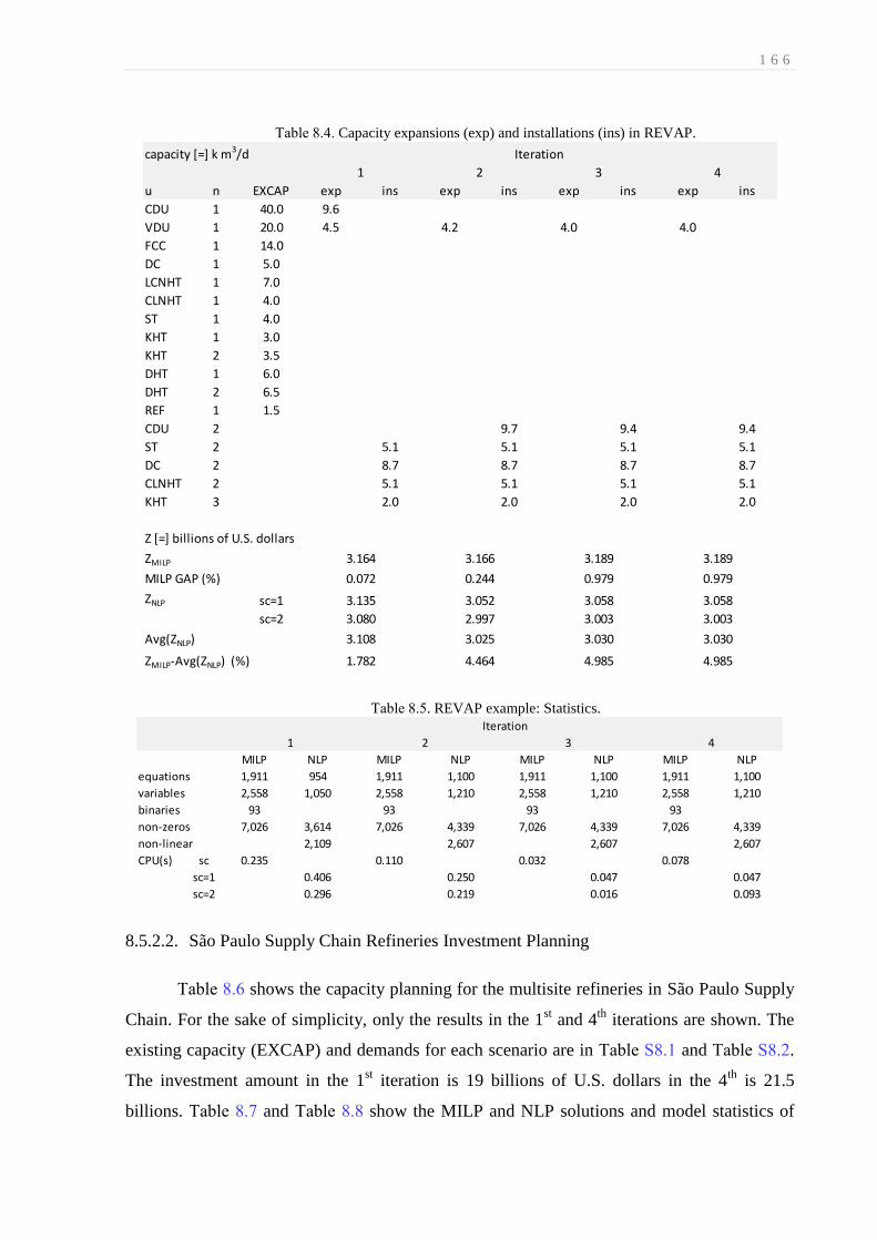
1 6 6

Table 8.4. Capacity expansions (exp) and installations (ins) in REVAP.

Table 8.5. REVAP example: Statistics.

São Paulo Supply Chain Refineries Investment Planning 8.5.2.2.

Table 8.6 shows the capacity planning for the multisite refineries in São Paulo Supply

Chain. For the sake of simplicity, only the results in the 1st and 4

th iterations are shown. The

existing capacity (EXCAP) and demands for each scenario are in Table S8.1 and Table S8.2.

The investment amount in the 1st iteration is 19 billions of U.S. dollars in the 4

th is 21.5

billions. Table 8.7 and Table 8.8 show the MILP and NLP solutions and model statistics of

capacity [=] k m3/d

u n EXCAP exp ins exp ins exp ins exp ins

CDU 1 40.0 9.6

VDU 1 20.0 4.5 4.2 4.0 4.0

FCC 1 14.0

DC 1 5.0

LCNHT 1 7.0

CLNHT 1 4.0

ST 1 4.0

KHT 1 3.0

KHT 2 3.5

DHT 1 6.0

DHT 2 6.5

REF 1 1.5

CDU 2 9.7 9.4 9.4

ST 2 5.1 5.1 5.1 5.1

DC 2 8.7 8.7 8.7 8.7

CLNHT 2 5.1 5.1 5.1 5.1

KHT 3 2.0 2.0 2.0 2.0

Z [=] billions of U.S. dollars

sc=1

sc=2

ZMILP-Avg(ZNLP) (%)

Avg(ZNLP) 3.030

3.003

3.058

0.979

Iteration

1

ZMILP

MILP GAP (%)

ZNLP

3.189 3.189

0.979

3.058

3.003

2 3 4

1.782

3.030

3.166

0.244

3.052

2.997

3.025

4.985

3.164

0.072

3.135

3.080

3.108

4.9854.464

MILP NLP MILP NLP MILP NLP MILP NLP

equations 1,911 954 1,911 1,100 1,911 1,100 1,911 1,100

variables 2,558 1,050 2,558 1,210 2,558 1,210 2,558 1,210

binaries 93 93 93 93

non-zeros 7,026 3,614 7,026 4,339 7,026 4,339 7,026 4,339

non-linear 2,109 2,607 2,607 2,607

CPU(s) sc 0.235 0.110 0.032 0.078

sc=1 0.406 0.250 0.047 0.047

sc=2 0.296 0.219 0.016 0.093

Iteration

1 2 3 4

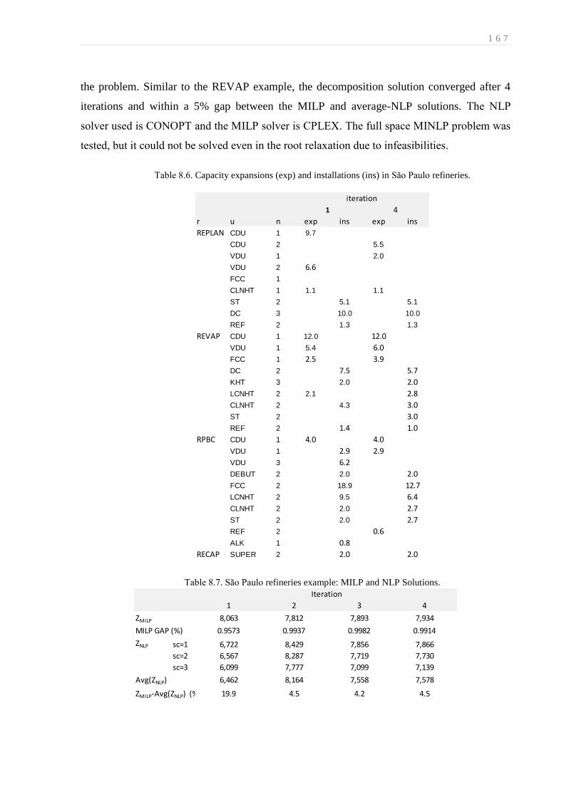
1 6 7

the problem. Similar to the REVAP example, the decomposition solution converged after 4

iterations and within a 5% gap between the MILP and average-NLP solutions. The NLP

solver used is CONOPT and the MILP solver is CPLEX. The full space MINLP problem was

tested, but it could not be solved even in the root relaxation due to infeasibilities.

Table 8.6. Capacity expansions (exp) and installations (ins) in São Paulo refineries.

Table 8.7. São Paulo refineries example: MILP and NLP Solutions.

r u n exp ins exp ins

REPLAN CDU 1 9.7

CDU 2 5.5

VDU 1 2.0

VDU 2 6.6

FCC 1

CLNHT 1 1.1 1.1

ST 2 5.1 5.1

DC 3 10.0 10.0

REF 2 1.3 1.3

REVAP CDU 1 12.0 12.0

VDU 1 5.4 6.0

FCC 1 2.5 3.9

DC 2 7.5 5.7

KHT 3 2.0 2.0

LCNHT 2 2.1 2.8

CLNHT 2 4.3 3.0

ST 2 3.0

REF 2 1.4 1.0

RPBC CDU 1 4.0 4.0

VDU 1 2.9 2.9

VDU 3 6.2

DEBUT 2 2.0 2.0

FCC 2 18.9 12.7

LCNHT 2 9.5 6.4

CLNHT 2 2.0 2.7

ST 2 2.0 2.7

REF 2 0.6

ALK 1 0.8

RECAP SUPER 2 2.0 2.0

41

iteration

ZMILP

MILP GAP (%)

ZNLP sc=1

sc=2

sc=3

Avg(ZNLP)

ZMILP-Avg(ZNLP) (%)

7,578

4.519.9

8,164

4.5

7,558

4.2

7,934

0.9914

7,866

7,730

7,139

7,893

0.9982

7,856

7,719

7,099

7,812

0.9937

8,429

8,287

7,777

8,063

0.9573

6,722

6,567

6,099

6,462

Iteration

1 2 3 4

1 6 8

Table 8.8. São Paulo refineries example: Statistics.

8.6. Conclusion

In summary, we have described how to iteratively solve a qualogistics or MINLP

capital investment problem using MILP and NLP sub-solvers configured in a coordinated

manner. This same technique can be applied to any advanced planning and scheduling

MINLP problem found in the process industries given our assertion that these types of

problems can be phenomenologically modeled using the QLQP attributes to concatenate the

sub problems. The major advantage of the partitioning and positioning approach is that each

sub problem can be independently and individually isolated and thoroughly investigated and

interrogated to troubleshoot and debug inconsistencies and unexpected solutions when they

exist. Existing MINLP and global optimizers are treated as black-boxes and if reliable and

relevant solutions are not obtained which is usually the case in practice, then little insight and

analysis is afforded back to the development and/or deployment user.

The integration between logistics and quality sub problems was implemented in a

complete oil-refinery investment planning problem to design new process frameworks as well

as to determine new process capacities. The processing uncertainties are intended to decrease

by more detailed formulation in crude dieting, process transformation and blending as a type

of preventative uncertainty management. Even though it is well recognized that the

decomposed procedure may generate merely sub-optimal feasible solutions, these are both

logistics and quality consistent, and the procedure is therefore significantly better than other

alternative usually employing manual trial and error simulation. It is important to highlight

that hopefully sometime in the near future, the pragmatic decomposition of the MINLP into

two simpler sub problems (logistics and quality) will not be required given the expected

evolution of MINLP solver technology. Yet, from an intelligent problem solving perspective,

dissecting a large problem into smaller sub problems (divide-and-conquer) can be a very

effective way of detecting, identifying and eliminating defects in the model and data supplied.

MILP NLP MILP NLP MILP NLP MILP NLP

equations 10,076 5,406 10,076 5,347 10,076 5,378 10,076 5,349

variables 13,782 5,932 13,782 5,870 13,782 5,899 13,782 5,870

binaries 213 213 213 213

non-zeros 36,950 24,825 36,950 25,515 36,950 24,606 36,950 24,547

non-linear 16,842 16,652 16,673 16,682

CPU(s) sc 2.969 4.281 3.375 3.407

sc=1 17.484 5.468 3.515 3.657

sc=2 20.718 0.219 4.235 4.203

sc=3 20.609 0.219 4.078 4.297

Iteration

1 2 3 4

1 6 9

Chapter 9

9. Conclusion and Future Work

In this thesis, we have described models and solution methods for the operational and

strategic decision-making of oil-refinery processes in a quantitative manner. In chapter 3, we

developed a model for the optimal nonlinear production planning of oil-refinery processes and

applied it to the Brazil’s oil-refining industry considering the hypothetical large refinery

REBRA to approximate the national multisite refineries production. In chapter 4, we

described a model for the optimal mixed-integer nonlinear strategic investment planning of

oil-refinery processes to determine overall capacity expansions per type of oil-refinery unit

considering the aggregated refinery REBRA. In chapter 5, we improved the swing-cut

modeling for better predicting quantity and quality values of distillate streams using a

property-based interfacial linear interpolation considering micro-cuts, hypotheticals, or

pseudocomponents distribution. We developed in chapter 6 a model that integrates distillate

stream cutpoints (initial and final boiling point temperatures) and fuel recipes optimization by

taking into account product evaporation data (ASTM) and its interconversion to TBP (and

vice-and-versa) to formulate the method using both monotonic interpolation. In chapter 7, a

generalized capital investment planning model that can be applied to small, medium, and

large size types of projects (repair, retrofit, revamps) formulates project setups and phases

using sequence-dependent setups in a scheduling environment. Finally, in chapter 8, we

outlined the phenomenological decomposition heuristic algorithm to solve the quantity-logic-

quality or qualogistics problem in a two-stage stochastic programming formulation with a

quantity-logic or mixed-integer problem in the first-stage defining the binary variables

(project setups) and NLP sub problems in the second-stage for the continuous variables

determination including quantity and quality balances.

9.1. Nonlinear Production Planning of Oil-Refinery Units for the Future Fuel Market in

Brazil: Process Design Scenario-Based Model.

In chapter 3, nonlinear operational planning model of oil-refinery processes defines

the production and import figures for Brazil’s future oil products market. The national

refineries are aggregated in a hypothetical large refinery to calculate overall volume balances

using as baseline the existing refineries and national data in 2013. The refineries under

construction and those in conceptual phases, starting up in 2016 and in 2020 respectively, are

1 7 0

added to the hypothetical large refinery (REBRA) to predict overall capacity increase to

match four different market demand scenarios.

The results for the 2013 scenario presented good precision with the national data

accumulated in the past 12 months until October, 2013 considering the gasoline and ethanol

for fueling market stabilization (GLNC scenario, see Figure 3.4). Crude import dependence to

yield more medium distillates is confirmed in around 12%, which is commonly ultralight

African oil, without including the crude imports for lubricant production of around 6%,

mostly from the Middle East. The GLNCETH scenario in 2013, discounting the ethanol to

gasoline market shift, demonstrates that before this move the country was free of gasoline

imports. The cause of this market shift was the ethanol price surge since 2009 that started as

conjectural situation related to sugar cane harvesting problems, due to droughts, and sugar

demand increase overseas, and it was intensified and is maintained by structural modification

in gasoline demands considering the economy increase from 2009 to 2012 in Brazil. As

ethanol is part of the retail gasoline between 18-25%, any further demand in gasoline directly

causes more demands for ethanol in the retail gasoline mix (GLNC).

In the baseline calculation for the existing refineries in 2013, higher prices for gasoline

and diesel are considered to yield a minimal margin of 0.5 US$/barrel. As seen in Table 3.7,

the current prices of these fuels are consuming around 14 million US$/d from PETROBRAS’

resources because of the import price differences when compared with the national Brazilian

market price.

By adding the refineries under construction (RNEST and COMPERJ-1) in the large

refinery REBRA in 2016, fuel imports (LPG, gasoline, jet fuel, and diesel) are minimized,

mainly diesel. RNEST production yields around 70% of diesel and a small increase in

gasoline and jet fuel production is from COMPERJ-1, basically from the first hydrocraking

unit to be installed in Brazil. Only in lower demand cases (4.2% p.a.) with investments in

projects to start up in 2020, jet fuel and diesel imports are reduced to zero, and the external

dependence of gasoline ceases in the investment cases only in the minimum import scenario

(4.2% p.a. and GLNCETH) with the conceptual projects performed with refitting.

In all demand scenarios with the conceptual phase projects built in 2020, the total size

of planned capacities of most units needs refitting. As example, for the overall planned CDU

capacity in 2020 (538 k m3/d), the throughputs idling figure of ~30−40 k m

3/d, suggesting that

1 7 1

a new site could be withdrawn from the future investment portfolio, given the expected

demand scenarios.

9.2. Mixed-Integer Nonlinear Production Planning of Oil-Refinery Units for the Future

Fuel Market in Brazil: Process Design Synthesis Model

Despite the importance of process design synthesis optimization within the oil-refinery

industry due to the intensive capital amount and complex processes involved, most

methodologies to determine facilities expansion of physical separation and chemical reaction

equipment in oil-refineries are based on a trial-and-error procedure. The oil-refinery process

design is manually tested to avoid mixed-integer models and they are usually formulated as

linear by considering crude oil diet, fuel recipe, and intermediate product quality as fixed

values, and the processing transformations are mostly delta-based formulae (f(x) = ax+b, a

and b as constant), all demanding continuous effort to update the overall parameter data in

order to maintain the accuracy of the simpler model. In chapter 3, the Brazil’s current and

future fuel production profiles are reproduced for fixed process design, in which a profit-

based approach for different fuel market scenarios considering the national crude oil

production by groups, fuel production, and imports of both crude and fuel is solved.

Alternatively, in the framework optimization-based approach presented in chapter 4, a

discrete optimization model finds the optimal process design creating a combinatorial

enumeration of setup variables to be explored by branch-and-bound methods. Continuous

variables are combined with these setup variables to evaluate the size of the projects by using

semi-continuous constraints, i.e., a continuous variable is zero or between bounds by the

appropriate selection of its respective binary variable. In the chapter, an MINLP model

determines the overall capacity expansion of existing units for the Brazilian large refinery

REBRA based on setup and sizing of projects in a multiperiod case. Similar to the results

found in chapter 3 for the 2020 scenarios, when the refineries under conceptual phase are

considered on-stream, the results in chapter 4 indicate the need to reevaluate the strategic

decisions considering the possible variation on future fuel demands.

In terms of modeling, comparing the results in 2020 from both NLP and the MINLP

methodologies, the former, considering a large number for unit throughput upper bounds,

results in unrealistic process design by decreasing the capacity of separation units (CDU and

VDU) and increasing the capacity of cracking units (HCC and DC). Unlike the NPV-based

MINLP methodology, the NLP problem does not take into account the investment constraints

1 7 2

in the profit-based maximization, so that larger profits are obtained with higher capacity of

low-to-high stream value units (HCC and DC), despite their more expensive investment costs.

Simplifications for considering five groups of crude, same cuts, and swing-cuts for all

CDU and VDU units, aggregated capacity per type of unit, averaged values for currency,

prices, demands, etc., all of them may influence the quality of the results. However, for the

national strategic planning level, the aggregated model and other simplifications addressed in

chapters 3 and 4 are sufficient for predicting the overall capacity expansion per type of oil-

refinery unit required to match the country’s future fuel demands and prevent the solution of

very large models by including all the refineries. The NLP operational planning formulation

(chapter 3) is used in a full space model integrated with the binary problem (chapter 4), which

can be solved in the aggregated approach instead of solving the multisite problem with 12 to

16 refineries considering the existing and new oil-refinery sites.

In both aggregated approaches, the NLP operational planning (chapter 3) and the

MINLP strategic planning (chapter 4) models, the future plans around the refining assets

expansion in Brazil cannot prevent the country’s fuel import in 2020, except in the lowest fuel

demand case (GLCNETH and 4.2% p.a.). Considering the country’s economy growth in the

past recent years, the retail gasoline/ethanol for fueling market steady-state, and the

uncertainties related to the national light crude production expansion from the new presalt

fields, the national oil-refining industry are reconfiguring proposed projects, as discussed in

Appendix 0A, and the approaches developed and the results obtained in chapters 3 and 4 may

guide investment decisions in the country.

9.3. Improved Swing-Cut Modeling for Planning and Scheduling of Oil-Refinery

Distillation Units

In chapter 5, we outlined an improvement to the conventional swing-cut modeling by

taking into account that the swing-cut fractions flowing to the light and heavy final-cuts,

distillates, or product-cuts have different properties that varies according to their proportions

between the light and heavy hypothetical interfaces (light-cut/swing-cut and swing-cut/heavy-

cut). The novel quality variation prediction for the light and heavy swing-cuts uses

pseudocomponents, hypotheticals or micro-cuts discretized into 10ºC increments of the crude

(crude-oil assay distribution curves) in a interfacial property-based linear interpolation.

Additional nonlinear relations (Equations 5.9 to 5.12) consider light and heavy swing-cut

1 7 3

amounts and properties of the hypothetical interfaces and the whole swing-cut (bulk

properties) to determine the different light and heavy swing-cut qualities.

An actual CDU operation with eighteen crude oils and three swing-cuts (see Figure

5.3) demonstrates property differences for final distillates in both the conventional and

improved swing-cut methods. The results show that the proposed improvement better predicts

specific gravity than sulfur content (see Figure 5.5 and Figure 5.6). This should be due to the

more nonlinear behavior in sulfur content, which is not well-captured in the linear

interpolation used. Although the small differences between the distillate qualities found in

both methods, when intensive values of the distillates, such as specific gravity and sulfur

content, are used in blend-shops and downstream units (such as hydrotreaters), these small

differences can avoid under or overestimation in operational settings when these intensive

values are extended considering stream volumes in pipelines or tanks.

In the planning example for production of different grades of diesel, the improved

swing-cut model yields higher profit if compared with the conventional method because of its

higher jet fuel production, which is provided by the lower specific gravity value for the light-

SW2 flowing to the kerosene final-cut (see Table 5.7 and Table 5.8). This difference

represented 3.3% in profit increase, which indicates 12.0 k US$/d or 4.380 million US$/y.

9.4. Distillation Blending and Cutpoint Temperature Optimization using Monotonic

Interpolation

Cutpoint optimization for distillation models in planning and scheduling problems

commonly use crude assay data considering simplifications in distillation process without

considering the thermodynamic and equilibrium relationships. In the swing-cut model, the

cutpoint optimization is approximated by amounts of light and heavy swing-cuts to determine

distillate flows with a given flexibility, which are used in rigorous process simulators to

define distillate temperature cutpoints (initial and final boiling points – IBP and FBP). These

points are defined as that temperature on the whole crude TBP that represents the limits

(upper and lower) of a fraction to be produced (Jones and Pujado, 2006), although simple

methods define cutpoint as the midpoint temperature between two adjacent “tails” (100% of

the lighter cut and 0% of the heavier cut).

The distillation blending and cutpoint optimization addressed in chapter 6 integrates

two major areas inside the oil-refineries, which is the distillate cutpoints (IBP and FBP) and

1 7 4

final blending recipes optimization. By interpolating experimental evaporation curves of the

distillate streams compounding the final blending pools, a novel adjustment or shifting

modeling modifies the distillate amounts and the whole evaporation curves to match quantity

and quality demands in fuel recipes optimization. The proposed methodology converts

evaporation curves from ASTM D86 to TBP temperatures and these points are converted to

cumulative evaporations using monotonic interpolation, where blending components are

linearly mixed in mass or volume basis to determine blended qualities such as evaporations.

These blended evaporations need to be converted back to TBP temperatures using another

monotonic interpolation, which is interconverted back to ASTM D86 to match fuel

specification (see Figure 6.3).

The illustrative example 6.1 represents a small optimization case (only 1 degree of

freedom) to compare three interpolation (linear, PCHP, Kruger) methods and to better

understand the interconversions of the distillation blending methodology. As seen, Kruger’s,

also known as constrained interpolation (Kruger, 2014), is more accurate with experimental

data, so this interpolation is used to reproduce all other examples in the chapter. Actual

PETROBRAS oil-refinery’s blend-shops comparing ASTM D86 temperatures for gasoline

and diesel products, examples 6.3 and 6.4 respectively, demonstrate that the proposed

methodology has better prediction than assuming ASTM D86 temperatures linearly blended

by volume (see Table 6.8 and Table 6.13). For the middle point (50% evaporation), the

ASTM D86 linear blending and the proposed distillation blending methodology are similar,

but for lower points (< 50%), the linear blending model overestimates the final blend values,

and for higher points (> 50%), they are underestimated.

In example 6.2, the distillation blending and cutpoint optimization case is

demonstrated by considering the distillate stream as a blending component to optimize the

front end, IBP, or T01 (1%) and/or back end, FBP, or T99 (99%) of the component TBP

distillation curves, updating the relative yields for other points of the adjusted or shifted

distillation curves. Physical phenomena that describe the behavior of the distillation towers

are captured in the experimental curves, which is a result of crude assays and fractionation

inside the towers. The model implies that the properties of the streams can be adjusted

without including the equations that describe the separation in a given distillation tower,

although the results must be used in further steps in rigorous process simulators to verify that

1 7 5

the modification is possible considering the actual tower operation. The results can also be

used as initial points in on-line optimization strategies.

Finally, in the diesel blending example, we can notice the addition of the ASTM D86

85% temperature which is required for the diesel product’s quality specification limits. As

there is no correlation to convert ASTM D86 85% to its respective TBP, this point is

calculated by interpolating the standard TBP temperatures at 1%, 10%, 30%, 50%, 70%, 90%,

99% and then creating another interpolation using these TBP temperatures as the abscissa and

the corresponding calculated ASTM D86 temperatures as the ordinate. The built-in

interpolation functions and the possibility to have their derivatives calculated automatically,

techniques found in IMPL (Industrial Modeling & Programming Language), becomes the

interconversions and interpolation quite easy to handle, which would be impossible or

extremely hard to implement by using other modeling languages in the market.

9.5. A General Approach for Capital Investment Planning using MILP and Sequence-

Dependent Setups

In chapter 7, a generalized model for capital investment planning of oil-refineries

using MILP is developed from a more realistic framework by considering project phases or

stages. The novel idea is to use sequence-dependent switchover modeling to represent the

construction, commission, and correction stages of the revamp, retrofit, and repair problem as

repetitive maintenance tasks or activities that are inserted between the "existing" and

"expanded" unit-operations. This allows generalizing the popular retrofit design synthesis

problem as a usual sequence-dependent changeover production planning or scheduling

problem including inventory and logistics details such as operating modes, run-lengths,

capacity expansions, conversion extensions, etc.

Although the addressed logic variables determine setups for installation and expansion

of oil-refinery units, this can be extended to procedures or tasks of units, pipelines, tanks, or

blenders. The project scheduling or investment analysis proposed is concerned with temporal

coordination for setups over time or startups of projects, in which admissible project

schedules must obey constraints such as precedence relations (investment, or tasks if included

production scheduling, cannot start unless another have been selected) and resource

restrictions (crude, capital, etc., scarce resources with limited capacities) (Wiesemann et al.,

2010).

1 7 6

The capital investment planning (CIP) is reformulated using capacity/capability and

capital as flows in a scheduling environment. The generalized CIP formulation can be applied

to any CIP problem found in the process industries which may require more scheduling

details to be considered. It can be easily modeled using the modeling and solving platform

IMPL, which is based on the superstructure shown in Figure 9.1 allowing the modeler or user

the ability to configure the problem using semantic variables such as flows, holdups, yields

and setups, startups, etc. without having to explicitly code the sets, parameters, variables, and

constraints required in all other algebraic modeling languages in the market. In the UOPSS

scheme, all links between the ports and the units have a binary variable to turn on or off the

existence of the shapes (units, ports, and streams) over time. This idea permits to solve

industrial-sized optimization problems in both planning and scheduling environments in

which the UOPSS shapes and procedures (each one having their own meaning) are integrated

over space and time considering renewable (units) and/or non-renewable resources (states).

Figure 9.1. UOPSS scheme.

In the motivating examples (expansion and installation of a unit) and in the oil-refinery

case for investments in CDU and VDU considering both expansion and installation, the

investment costs consider fixed and varying terms, in which capital and capacity are treated

using holdups, flows, tanks, etc. However, in the example taken from Jackson & Grossmann

(2002) with 3 feeds (A,B,C) and 2 product materials (D,E) with 3 processes (Figure 7.7),

expanded (capacity increase) or extended (conversion increase) or both projects can be

performed with fixed capacity/capability and costs. In a total of three time periods, 36 binary

variables are necessary to formulate the problem in both big-M and convex-hull approaches,

although 154 binary variables are necessary in our proposed approach, which was solved with

CPLEX in less than 0.25-seconds to provably optimal.

1 7 7

9.6. Phenomenological Decomposition Heuristic for Process Design Synthesis of Oil-

Refinery Units

The full space MINLP or quantity-logic-quality (QLQ) models are still challenging for

industrial-sized problems, because considering all three types of QLQ variables and

constraints simultaneously results in both a discrete and nonlinear formulation due to the

binary and integer nature of the logic variables and the multilinear terms of quantity times

quality. Fortunately, first solving the problem for logistics and then for quality is actually

somewhat intuitive and natural given that if the quantity and logic details are not feasible (or

consistent) then the quantity and quality details will also not be feasible, and even immaterial.

Hence, this provides some level of intelligent problem solving structure by allowing for a

staged or progressive workflow when making production or manufacturing decisions.

The alternative but heuristic approach proposed in chapter 8 is to successively solve

the logistics (quantity and logic) MILP sub problem first, fix the logic variables at their

solution values and then solve the quality (quantity and quality) NLP sub problem second.

After this solution is found, the quality variables can be fixed and/or updated yields (recipes,

ratios, recoveries, etc.) can be computed and the logistics problem resolved. This procedure

can be repeated until acceptable convergence is achieved or it is locally or globally infeasible.

The proposed two-stage stochastic programming framework, which is appropriate for

the integration of the NLP operational and MILP strategic decision-making, reduces

uncertainties related to the process with recourse in crude-oil diet and yields, which are

updated in the strategic decision after their determination in the NLP operational sub

problems for each demand scenario. The phenomenological decomposition method can be

applied to any quantity-logic-quality MINLP model to segregate it in two solutions. As we

propose, the nonlinearities from the processing and blending equations are solved separately

from the logic equations, so that the quantity-quality nonlinearity or phenomena is

decomposed to solve the quantity and logic optimization and then the quantity and quality

problem.

The oil-refinery example considers REVAP’s existing units in order to determine

expansion and installation of units as seen in Table 8.4. Although the gap between the MILP

and the average value of the NLP sub problems (considering the scenarios) is within 5%

since the 1st iteration, the problem converged after 4 iterations when the results (objective

function, new capacities, etc.) stop to change. The CDU investment after the 1st iteration

1 7 8

moved from expansion to installation and the new capacities for CDU and VDU converged in

the 4th

iteration.

9.7. Contributions of the Thesis

The main contributions of the thesis are summarized as follows:

1. An NLP formulation for operational planning of oil-refinery processes. The formulation is

proposed in chapter 3 and has been applied to calculate fuel production in Brazil’s oil-refining

industry considering the national existing refineries in 2013 aggregated in the hypothetical

large refinery REBRA, where the future refineries were added to determine the required

overall unit throughputs in 2020 to match different market scenarios.

2. An MINLP formulation for strategic planning of oil-refinery processes integrating the

operational and strategic layers in a full space model. A discrete formulation defines the types

of units to invest and the overall size of the new capacities for the Brazil’s oil-refining

industry considering nonlinearities from processing and blending constraints.

3. An improved swing-cut model by taking into account that the light and heavy swing-cut

fractions have different qualities. The novel approach uses micro-cuts, hypotheticals, or

pseudocomponents to infer the quality distribution along the whole swing-cut. The additional

correlations to predict the light and heavy swing-cut properties consider swing-cut bulk

properties, light and heavy swing-cut amounts, and properties in the hypothetical interfaces

between the swing-cut and its lighter (upper) and heavier (lower) adjacent cut streams

4. A novel technique to optimize distillate stream cutpoints (initial and final boiling points)

integrated with fuel recipes optimization. Experimental data of evaporation curves is

interpolated in monotonic interpolation and a new adjustment or shifting modeling is

addressed to modify the distillation curves considering distillates’ initial and final boiling

point temperature changes.

5. A generalized capital investment planning introduces a novel modeling for optimization of

project setups and phases using sequence-dependent logic, where capital and capacity are

treated as flows in a scheduling environment.

6. A tailored decomposition scheme to solve the process design or logistics problem in a

stochastic MILP approach considering probabilities over demand scenarios (first stage) from

where the defined process design is validated in NLP sub problems for each scenario (second

1 7 9

stage), with recourse in crude-oil diet and unit yields which are updated in the MILP problem

every each MILP-NLP iteration.

9.8. Recommendations for Future Work

9.8.1. Modeling of operational decision-making

1. In chapter 3, we used a complete oil-refinery network to determine production amounts

considering modeling in processing and blending. Development of processing models to

predict product quantity and quality variations for types of units unaddressed in this work

such as delayed coker, reformer, and hydrocracker units would be interesting to increase the

accuracy of the production. Evaluation around the computational efforts over processing and

blending models, each one added step-by-step in a problem, may guide one to define the best

set of models to include considering their solution burdens.

2. In chapter 5, improving the distillate predictions, the conventional swing-cut method is

reformulated to include quality variation in the light and heavy swing-cut fractions using

pseudocomponents or micro-cuts distribution of the crude. The approach mixes the micro-cuts

of each crude oil to form cuts and swing-cuts inside the towers considering known their

temperature cut ranges. Then, these internals are blended to yield final cuts or distillates.

Other approach that firstly mixes the micro-cuts from the crude pool, creating large blended

micro-cuts and then cutting them to form the internal cuts and swing-cuts, can also be

explored. The internals (cuts and swing-cuts) modeling can be avoided by creating micro-

swing-cuts that mix with their adjacent micro-cuts to form the final cuts directly. These

micro-cuts, pseudocomponents or hypos (hypothetical species) can also be used either in

interpolation or in regressed data models using cumulative distributive functions (CDF),

which demands temperature cutpoint determination instead of swing-cut amounts to

approximate the distillate variation. All mentioned models are depicted in Figure 9.2.

1 8 0

Figure 9.2. Micro-cuts, hypos (hypothetical species), or pseudocomponents modeling in distillation

problems.

3. In chapter 6, distillation temperature cutpoints and blending recipes are optimized together

by converting experimental distillation curves from ASTM to TBP and then in monotonic

interpolation to be used in a novel adjustment and shifting modeling considering initial and

final boiling points (IBP and FBP) temperatures of the distillates. Three regions are modeled

in the evaporation curves (front end: 1% to 10%; middle: 10% to 90%; and back end: 90% to

99%), although it can be detailed in more regions to better assess the nonlinearities of the

curves (see Figure 6.4). Also, the modeling can be extended to FCC and DC main

fractionators and as well as to hydrotreaters.

4. In chapter 6, the properties of the streams leaving the upstream units cannot be adjusted for

one stream independently of the other streams. Large portion of these streams are produced by

multi-product distillation towers (e.g. atmospheric distillation or FCC main fractionator), so

changing properties of one stream results in changes of the properties of the remaining

streams which are produced by the same tower. So, integration of two adjacent distillate

streams would be interesting to model.

5. In chapter 6, the cutpoint optimization is simply based on properties that would be the most

advantageous from the blending viewpoint. Such optimization is always a trade-off between

1 8 1

energy consumed to accomplish given separation and the incremental benefits accomplished

by changing the stream properties, which is not included in the proposed optimization model.

Even if one argues that the incremental energy costs are always lower than the benefits from

producing incremental amounts of better quality blending streams, one ends up with an

“overshoot” since the cost of incremental energy is treated as zero. So, a robust solution

would be the integration of energy balances in the problem.

6. The operational planning formulation used throughout the thesis is considered as a pre-

scheduling problem due to its material balance calculation in cubic meter per day, but it is

modeled in LP or NLP approaches without including scheduling operations. Discrete

optimization over these operations can be included to account selection of tasks and their

transitions in tanks, blenders or pipelines. This scheduling operation addition may not

influence in the strategic evaluation or gains, but at least validates the production feasibility.

7. Extending the production by including logistics movements inside and outside the refinery

boundaries can improve the overall modeling by integrating crude distribution, crude

processing, and fuels distribution, which are the productive related branches in between the

commercial segments (crude purchasing and fuel sales).

9.8.2. Modeling of strategic decision-making

1. The strategic and operational decision-making addressed in chapter 8 (PDH) can be

extended to the case with all 12 existing refineries in Brazil in order to compare with the

planned capacity for the new sites, considering the refineries under construction and in

conceptual phase. In these large examples would be necessary other types of decomposition

such as in time and space.

2. The strategic decision-making can be extended to the entire supply chain as in the

operational problem. Decisions on which units, tanks, pipelines, blenders, etc. to expand or

newly build can be included to consider the restructuring for a set of sites (refineries,

terminals, etc.).

3. The strategic decision-making can be extended to determine new sites such as refineries

and terminals by adding the possible units, tanks, and pipelines in the superstructure. Regional

differences in terms of taxes, environmental constraints, and logistics costs, considering crude

and fuel distribution, may be valuable information to include before a new site determination.

1 8 2

4. The power-law formula for equipment cost versus size can be linearized in three regions

(initial, middle, and final) (see Appendix 0B), where the middle region is considered in the

calculations. Considering the investment coefficients (alpha and beta) differences related to

the size of the new capacity, these numbers can be updated every each MILP-NLP iteration

after the capacity determination within the MILP problem.

5. For simplification, in the strategic planning models in chapters 4 and 8, an investment time

interval of several years is considered for the calculation without taking into account the

annual projects approving as commonly performed within the oil-refining companies. A

reformulation considering annual project approving may be explored, although the increase in

the number of binary variables will elevate the computational burden.

6. Considering that some companies have oil-refineries around the world such as Exxon, Shell

and Total, an oil-refining investment world map might guide the companies to choose the best

countries for investing in oil refinement. It can be done using the GCIP (chapter 7) and PDH

(chapter 8) models, and considering investment cost profile per region, national information

on oil production, refining capacity, oil product demands, transportation costs, etc. An

example to reproduce would be the KNPC (Kuwait oil company) refineries, where process

details of their 3 refineries can be found in their website.

7. Another kind of uncertainty such as in project startup schedule, crude oil production, and

investment resources can be addressed. The risk measurement as applied in the financial

strategy studies in PETROBRAS today would allow the introduction of risk measure concepts

like Value at Risk (VaR) or Conditional Value at Risk (CVaR) to the strategic problem.

8. An optimization strategy for integration of strategic, tactical, and operational decision-

making levels in vertical (multi-level) and horizontal (multi-entity) realms (Figure 9.3) would

be explored to address an industrial solution covering these areas that is still missing the

world.

Figure 9.3. Strategic, tactical and, operational decision-making levels.

1 8 3

Appendix A: Investment Strategies for the Future Fuel Market in Brazil

Oil industry investments in Brazil are growing at an unprecedented pace. New oil

reserves, significant increases in fuel demands, and new and more stringent fuel specifications

have accounted for US$ 300 billion in investments over the past 10 years. The progress of the

oil and fuel production as result of these investments is analyzed considering the current and

proposed alternatives to match both quantity and quality demands for the future fuel market in

Brazil. Today, two grassroots refineries under construction and more three additional sites in

conceptual phase are planned to prevent deficit in crude-oil derivatives of around 30% in

2020, as recent estimate in the country. However, the future perspectives about the national

oil refining capacity expansion deal with uncertainties around government policies, oil

production, gasoline-ethanol costumer preference, and fuel demands, which are leading to

investment reanalysis. Additionally, the economic logic may postpone investments in

downstream to raise capital to higher project returns in upstream, and may the persistent

economic world crisis started in 2008 and the unconventional Brazilian fuel policies change

business expectations. As will be seen, half of the capital planned in downstream in the next

cycle of investments, US$ 20.6 billion, is being reevaluated in several segments.

A1.Introduction

The economic growth in Brazil over the past 10 years, has led the country to critical

levels in terms of fuel demands. Analyzing this situation in progress, Tavares et al. (2005)

proposed market scenario simulation considering oil refining assets or facilities expansion

criteria in the country, which indicate that the investments required for the Brazilian oil

refining sector are over and above those allocated. In their work, the national oil refining

expansion strategies consider (1) energy security by reducing imports and vulnerability of key

products (e.g., gasoline, jet fuel, and diesel), (2) profit maximization by boosting the output of

higher value oil products (e.g., jet fuel, and diesel), (3) national oil processing priority by

reducing exports of heavy acid oil (e.g., metallurgic protection in crude distillation units, and

new delayed coker units), and (4) petrochemical integration (e.g., integrated refinery and

petrochemical complex projects). They concluded that the decision to invest in the oil refining

sector in Brazil depends on local infrastructure conditions, environmental constraints, fuel

specifications, companies’ strategies, steady growth in fuel demands and the definition of

government policies that eases institutional risks.

1 8 4

Facilities planning alternatives for the Brazilian oil refining industry is shown in

chapters 3 and 4, where are proposed simulation- and optimization-based methodologies to

expand the overall oil-refinery capacity in the country. In these modeling, the national

refineries are aggregated in one hypothetical large refinery to evaluate the overall capacity

expansion per type of process unit using mathematical programming approaches. Both

methodologies indicate alterations in the country’s oil-refining investment plans and outline

new required capacity expansion for 12 different types of process unit.

This work analyzes the development of the oil refining industry in Brazil from its

historical evolution as well as the future perspectives for investments in this sector in the

country. In section 2, the past and future of the Brazil’s oil industry investments are

interconnected to the oil production and processing growth in terms of both quantity and

quality. In section 3, the capital amounts being reevaluated by downstream segments as a

consequence of the new national oil industry scenario, and the deleterious gasoline and diesel

controlled pricing policy are shown. In section 4, the economic and political scenarios

currently faced by the nation and by the national oil and energy company PETROBRAS are

highlighted. In addition, the needs to develop high performance strategic investment decision-

making models to handle with uncertainties, nonlinearities from oil-refining processes, and

the unusual fuel market in terms of pricing and flex-fuel fleet market in Brazil are remarked.

Final comments and policy implications are presented in section 5.

A2. Brazilian Oil Industry: Past, Present and Future

A2.1. Oil industry investments in Brazil

Founded in 1953, Brazil’s national oil company, PETROBRAS, monopolized the oil

industry (with the exception of fuels retailing), until the “market flexibilization” in 1997,

when the country became open to non-governmental activities in the sector. As a consequence

of the lack of oil resources and small-sized fuel market, national oil investments (mainly in

downstream) stood below US$ 2 billion per year until 1977, when the investments in

upstream arose as a result of the Second Oil Crisis in the aftermath of the War between Iran

and Iraq. After this period, the expense with oil imports increased more than ten times and

reached US$ 10 billion in 1981. To overcome this unbalanced situation, investments in

upstream activities were expanded and concentrated in the Campos Basin exploration,

discovered in 1977, thereby switching the investments priority from the downstream to the

upstream sector - a trend that endures to this day. The national oil production expanded from

1 8 5

167 kbpd in 1979 to 630 kbpd in 1990, and the expense with oil imports decreased to US$ 3

billion per year in 1990 (PETROBRAS, 2013a). Additionally, governmental programs to

substitute gasoline with ethanol appeared as an option to reduce the external oil dependence

since that time, ethanol has become an important compound in the country’s fuel scenario.

After the market flexibilization, the increase of nonpublic investments, both national

and foreign, to compete in any oil activity promoted a surge in investments in the oil sector.

Over the past 10 years, PETROBRAS itself expanded its investments from US$ 5 to almost

US$ 45 billion per year, as shown in Figure A1, which, to the best of our knowledge, can be

considered a growth in capital for investments never-before-seen in any company worldwide.

In this period (2002-2012), investments ensured significant deep water fields exploration and

expanded the oil-refining assets in order to accomplish the first cycle of investments after the

flexibilization of the market. Investments in downstream accounted for more than 35% of the

entire amount by the end of the period, which is a significant departure from the historical

trend, with upstream representing more than 60%. The second cycle (2013-2020) focuses both

on the downstream required projects, which includes the startup of new refineries, and,

primarily, on expanding the exploration of new fields recently discovered in the so-called

presalt reserves. Within the next five years (2014-2018), PETROBRAS plans to invest US$

220.6 billion, an average of US$ 44.12 billion per year with 70% in upstream and 18% in

downstream (PETROBRAS, 2014a).

Figure A1. Historical and future investments in PETROBRAS (PETROBRAS, 2014a,2014b).

1 8 6

Despite the current and probably even with the future fuel deficit in the country, the

upstream sector emerges as a definite priority in the investment portfolio due to the lack of

enough capital to be invested in all necessary projects throughout all sectors and also due to

the fact that the upstream margins are considerably higher than the downstream ones.

The oil-refining assets or facilities expansion performed in the first cycle and those in

executions or in the conceptual phases in the second cycle aim to supply the growing fuel

demands and to increase the processing of domestic oil, both of which contribute to a

reduction in imports. Additionally, new specifications for gasoline and diesel, mainly related

to the reduction of their sulfur concentration, demand an extension of the investment expenses

without adding any quantity of fuels, since this only guarantees their new qualities

specifications. In the existing refineries, investment projects revamped and installed several

units. Around thirty-two new units were installed such as delayed cokers to convert fuel oil

into higher value products, hydrotreaters to reduce sulfur concentration in gasoline and diesel,

and reforming units to guarantee the gasoline octane number specification (PETROBRAS,

2009). For the next few years, the fuels market scenario in Brazil demands new projects to

prevent a deficit in crude-oil derivatives (fuels and lubricants) of around 30% in 2020 as

shown is Figure 3.1. The downstream investments portfolio includes new refineries adding

1,595 kbpd to the 2,103 kbpd attained in 2013 by the existing ones, considering crude

distillation capacity.

A2.2. National oil production and processing evolution

The historical evolution of the national oil production can be segmented into four

phases: onshore, flat water, deep water and Pre-Salt. Oil production began on onshore fields

in the Brazilian northeast region known as Reconcavo Baiano and the production was modest

until the deep water Campos Basin discovery even with the flat water fields along the east

coast. Only after the Albacora production startup in 1990 and later with other huge fields such

as Roncador, Barracuda and especially Marlim, all of them in deep waters, did oil production

grow significantly from 1994 until its stabilization in 2.1 million bpd in 2010 as seen in

Figure A2. The last phase brought huge expectations when in 2006 the discovery of an

enormous offshore oil basin, known as presalt, was reported. This basin lies over deeper than

the deep water fields, that is, around 6-8 km below the ocean floor, and already accounted for

14% of all national oil production in 2012 (PETROBRAS, 2013c).

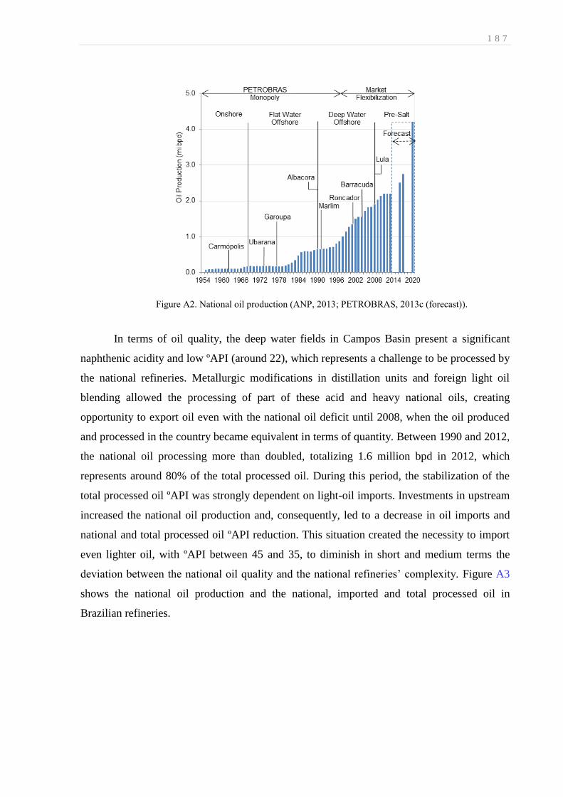
1 8 7

Figure A2. National oil production (ANP, 2013; PETROBRAS, 2013c (forecast)).

In terms of oil quality, the deep water fields in Campos Basin present a significant

naphthenic acidity and low ºAPI (around 22), which represents a challenge to be processed by

the national refineries. Metallurgic modifications in distillation units and foreign light oil

blending allowed the processing of part of these acid and heavy national oils, creating

opportunity to export oil even with the national oil deficit until 2008, when the oil produced

and processed in the country became equivalent in terms of quantity. Between 1990 and 2012,

the national oil processing more than doubled, totalizing 1.6 million bpd in 2012, which

represents around 80% of the total processed oil. During this period, the stabilization of the

total processed oil ºAPI was strongly dependent on light-oil imports. Investments in upstream

increased the national oil production and, consequently, led to a decrease in oil imports and

national and total processed oil ºAPI reduction. This situation created the necessity to import

even lighter oil, with ºAPI between 45 and 35, to diminish in short and medium terms the

deviation between the national oil quality and the national refineries’ complexity. Figure A3

shows the national oil production and the national, imported and total processed oil in

Brazilian refineries.

1 8 8

Figure A3. National oil production and national, imported and total oil processed and their ºAPI (ANP, 2013).

The first cycle of investments in the downstream sector after the flexibilization of the

market projected the refining assets modifications considering the ºAPI decrease scenario,

based on Campos Basin crudes production. But after the light-oil discovery in the oceanic

sub-salt layer along the Brazilian southeast coast, the national oil ºAPI projection increased.

The Pre-Salt fields gave way to a new scenario in Brazil, not only due to the expected rise in

oil production, but also because the new fields are compounded by crude-oils lighter than the

oils in the Campus Basin (around 32 ºAPI) creating the opportunity to reduce or even cease

oil imports altogether in the future.

A2.3. Fuel quantity and quality improvements

As a consequence of historical and recent situation, the needs for higher quantity and

better quality of fuel drove huge investments in the downstream sector in the past 10 years in

Brazil. Considering the main fuels, the historical deficit in LPG (Liquid Petroleum Gas) and

diesel (DSL) have structural reasons. LPG imports are the result of low natural gas reserves

and a deficient pipeline infrastructure, made worse by the existence of distant countryside

regions in a continental country like Brazil. The diesel deficit has its origins in past political

decisions, whereby road transportation was given priority throughout the country. Today, this

deficit prevents the market from producing small and medium cars fueled by diesel.

Jet fuel (JET) and gasoline imports increase started as a conjectural situation that

seems to have led to a structural problem. Growing domestic and international tourism

increased the demands for jet fuel, which are expected to reach critical levels or even

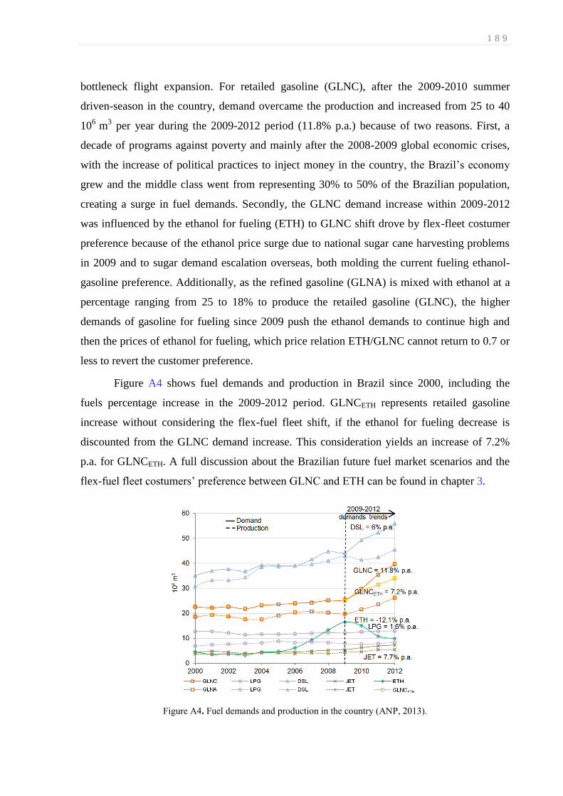
1 8 9

bottleneck flight expansion. For retailed gasoline (GLNC), after the 2009-2010 summer

driven-season in the country, demand overcame the production and increased from 25 to 40

106

m3 per year during the 2009-2012 period (11.8% p.a.) because of two reasons. First, a

decade of programs against poverty and mainly after the 2008-2009 global economic crises,

with the increase of political practices to inject money in the country, the Brazil’s economy

grew and the middle class went from representing 30% to 50% of the Brazilian population,

creating a surge in fuel demands. Secondly, the GLNC demand increase within 2009-2012

was influenced by the ethanol for fueling (ETH) to GLNC shift drove by flex-fleet costumer

preference because of the ethanol price surge due to national sugar cane harvesting problems

in 2009 and to sugar demand escalation overseas, both molding the current fueling ethanol-

gasoline preference. Additionally, as the refined gasoline (GLNA) is mixed with ethanol at a

percentage ranging from 25 to 18% to produce the retailed gasoline (GLNC), the higher

demands of gasoline for fueling since 2009 push the ethanol demands to continue high and

then the prices of ethanol for fueling, which price relation ETH/GLNC cannot return to 0.7 or

less to revert the customer preference.

Figure A4 shows fuel demands and production in Brazil since 2000, including the

fuels percentage increase in the 2009-2012 period. GLNCETH represents retailed gasoline

increase without considering the flex-fuel fleet shift, if the ethanol for fueling decrease is

discounted from the GLNC demand increase. This consideration yields an increase of 7.2%

p.a. for GLNCETH. A full discussion about the Brazilian future fuel market scenarios and the

flex-fuel fleet costumers’ preference between GLNC and ETH can be found in chapter 3.

Figure A4. Fuel demands and production in the country (ANP, 2013).

1 9 0

In terms of fuel quality, in 1986 the Brazilian Environmental Agency established a

national program to control air pollution from automobiles. This government program focuses

on gradually reducing automobiles emission with exhaust gases mitigation in new fleets, more

efficient motor combustion and fuel quality improvements to decrease sulfur and nitrogen

contaminants, which form, respectively, SOx and NOx. Because of the lower sulfur

concentration particulates reduction is also achieved. The national program for diesel is

shifting the S1800 (1800 ppm of sulfur in weight) market to S500 and S10 (10 and 500

wppm, respectively), as shown in Figure A5. The lower sulfur grades of diesel S10 and S500

will represent 80.37% of the market. After 2014, the S1800 diesel will be fueling only engines

used in so-called off-road transport, like tractor and train fleets. Additionally, the gasoline

specification after 2014 will be changed from 1000 to 50 wppm in sulfur, which demands the

installation of new hydrotreaters for distilled, coker and cracked naphtha.

Figure A5. Diesel grades evolution (MPF, 2013).

In addition to altering the refining process to produce ultra-low sulfur diesel (S10),

there will be investments in logistics for the new diesel grades. The pipelines and tanks

handling S10 should be dedicated exclusively to this service in order to prevent sulfur

contamination from other grades. Other specifications are also changing like specific gravity

and distillation temperature, both to reduce heavy fractions on ultra-low sulfur diesel. Other

diesel variant, the S50 (50 wppm S), was discontinued to avoid investments in two logistics

assets for diesel variants so close (S10 and S50). The S50 initial existence came from the

necessity to produce low sulfur diesel compatible with the refining assets in 2009. It was

obtained with operational adjustments and improvements in hydrotreaters efficiency using

1 9 1

catalyst bed with higher activities, lower spatial velocity and feed management. Only with the

new hydrotreating units the refineries will be able to produce S10 demanded by the country,

because of their higher severity in dealing with higher pressure and temperature, which

demanded higher investments to build hydrotreaters with large thickness and metallurgy and

reactors more specialized.

The future refining scenario needs to complete the investments to increase fuels supply

and to satisfy the gasoline and diesel new specifications mainly related to the sulfur reduction.

Other tendencies like to reduce the nitrogen content in jet fuel and to increase the octane

number in gasoline may demand more investments in the sector. Changes in premises in the

second cycle (started in 2013) consider the future national oil to be produced lighter than in

the first cycle because of the presalt reserves. Also, the market stabilization considering the

gasoline-ethanol costumer dynamics and the boosting demands throughout the fuels are

leading to projects reanalyzes.

A3. National Strategies and Pricing Policy for Fuels

A3.1. Downstream investments reevaluation

The refineries currently under construction, RNEST and COMPERJ-1, were projected

to privilege diesel production. Exogenously, its higher price in comparison with jet fuel and

gasoline, and endogenously, the road-based transport predominance in the country, accounted

for the diesel preference when it came to investment decisions. However, considering the

boost in other fuel demands due to the Brazilian economic growth and the ethanol for fueling

to retail gasoline market shift, doubts have been raised concerning the application of the same

emphasis on diesel production in the projects in conceptual phase (Premium I, Premium II and

COMPERJ-2). Additionally, the presalt production may change the refining design outline,

replacing the African ultra-light and Middle East paraffinic crudes, currently used to provide

higher yields in medium distillates and lubricants, respectively. Figure A6 shows the foreseen

investments for the period 2013-2017 in PETROBRAS’ downstream sector. As shown, about

50% of total capital planned for the projects is being reevaluated.

1 9 2

Figure A6. Downstream investment portfolio reevaluation in Brazil (PETROBRAS, 2013a).

The refining assets growth amount under reevaluation represents a large and complex

refinery in Brazil. The operational improvements to increase the efficiency of obsolete

equipment and operational debottlenecking in on-site and off-site assets proceed essentially as

planned. The investments related to fuel market specifications are mandatory and possibly the

projects in this segment related to the reduced asset expansion are being reevaluated. Other

segments in reevaluation are associated with Brazilian peculiarities. The investments to

increase the national crude processing percentage are related to the Brazilian crude’s most

difficult characteristic, its acidity. Possibly, the new perspective about the increase of national

light oil from the presalt reserves is restraining investments in this topic. On the other hand,

investments in the ship fleet and in ethanol logistics, priorities aiming at reducing foreign fleet

contracts and supporting the gasoline-ethanol market expansion respectively, may have a

residual reduction as well as the investments related to operational improvements, since the

current logistics bottlenecks in Brazil threaten companies’ profitability.

Finally, the petrochemical disinvestments are likely to be accomplished, since this is

part of PETROBRAS’ new strategy. Despite that, the high import levels of petrochemicals

can be considered a national problem, and estimates of required investments in the 2011-2020

period reach figures of around US$ 87-167 billion for petrochemicals to face the current

situation and the expected increase in demand, which came to 29% in 2009-2010 (Pinto,

2012). PETROBRAS’ prior experience in petrochemicals was based on the purchase of assets

and minority participations in petrochemical companies. The strategic decision to build

1 9 3

COMPERJ-2 as a petrochemical complex could not be sustained due to lack of capital to

simultaneously invest in the necessary and more profitable downstream and upstream

portfolios, respectively.

A3.2. Gasoline and Diesel Pricing Policies

The Brazilian state has been rolling an intensive interventionism policy for fuel pricing

with the excuse that the weight of gasoline and diesel in the national inflation calculation is

significant. Since the flexibilization of the market in 1997, state intervention in fuel pricing

was being reduced directly, although the major control of the national oil and energy company

PETROBRAS by the 50.2% ordinary state-owned stocks indirectly maintain the state

interventionism. As a consequence of this, the refining activity in Brazil today is not being

lucrative. This is a well-known situation due to the national gasoline and diesel producer

lower price in comparison with import prices. Although the LPG and jet fuel imports in the

country, they do not damage the company’s profitability because in Brazil the controlled LPG

price is similar to the international practices and the jet fuel prices are not controlled by the

country. However, for gasoline and diesel the difference between the national producer prices

and the imports is absorbed by PETROBRAS. The Brazilian Center of Infrastructure

estimates losses of 2.2 billions of U.S. dollars from January to May, 2013 (14.379 million

US$/d) considering the difference between the producer prices for gasoline and diesel in US

Gulf Coast and Brazil (Globo, 2013). In chapter 3, the proposed calculation estimates losses

of 16.702 million US$/d considering the pricing scenario of the past 12 months until October,

2013.

In Figure A7 the price percentage for gasoline and diesel in Brazil and US are

compared in terms of distribution & marketing, taxes and producer amounts. In both

countries, the percentage for distribution & marketing are similar, but the taxes in Brazil in

comparison to US is almost a double for gasoline and more than double for diesel. In Brazil

the taxes on these fuels are split between national and state taxes, representing, respectively,

7% and 28% of gasoline price and 6% and 14% of diesel price (PETROBRAS, 2014b). In

Brazil the producer percentage for gasoline is compound by ethanol mixed at 25% with

refined gasoline, and for diesel is compound by biodiesel mixed at 6% with refined diesel, so

the total producer amount for gasoline is 48% and for diesel is 65% of their final price

percentage. In the US, the producer percentage for gasoline and diesel is 76% and 77%,

respectively (EIA, 2014). This unusual controlled prices situation inside the oil-refining

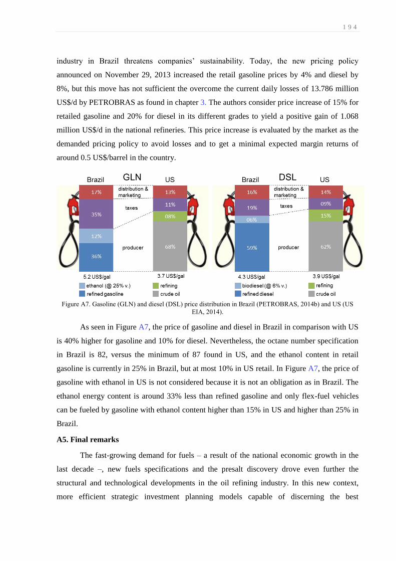
1 9 4

industry in Brazil threatens companies’ sustainability. Today, the new pricing policy

announced on November 29, 2013 increased the retail gasoline prices by 4% and diesel by

8%, but this move has not sufficient the overcome the current daily losses of 13.786 million

US$/d by PETROBRAS as found in chapter 3. The authors consider price increase of 15% for

retailed gasoline and 20% for diesel in its different grades to yield a positive gain of 1.068

million US$/d in the national refineries. This price increase is evaluated by the market as the

demanded pricing policy to avoid losses and to get a minimal expected margin returns of

around 0.5 US$/barrel in the country.

Figure A7. Gasoline (GLN) and diesel (DSL) price distribution in Brazil (PETROBRAS, 2014b) and US (US

EIA, 2014).

As seen in Figure A7, the price of gasoline and diesel in Brazil in comparison with US

is 40% higher for gasoline and 10% for diesel. Nevertheless, the octane number specification

in Brazil is 82, versus the minimum of 87 found in US, and the ethanol content in retail

gasoline is currently in 25% in Brazil, but at most 10% in US retail. In Figure A7, the price of

gasoline with ethanol in US is not considered because it is not an obligation as in Brazil. The

ethanol energy content is around 33% less than refined gasoline and only flex-fuel vehicles

can be fueled by gasoline with ethanol content higher than 15% in US and higher than 25% in

Brazil.

A5. Final remarks

The fast-growing demand for fuels – a result of the national economic growth in the

last decade –, new fuels specifications and the presalt discovery drove even further the

structural and technological developments in the oil refining industry. In this new context,

more efficient strategic investment planning models capable of discerning the best

1 9 5

investments portfolio, are being developed in the country. It has transpired not only due to the

monopoly being broken and the consequent investments surge, but also as a result of the need

to adequately refit the existing refining and logistics structures to avoid unnecessary expenses,

especially to maintain the company’s competitiveness. Investments in production and logistics

facilities considering the new fuel consumption rate and the unpredictable gasoline-ethanol

demand shift driven by the flex-fuel consumers is necessary to provide the future fuel market

needs and the required supply chain structure in the country. Additional challenges to produce

different diesel grades in terms of sulfur concentration should be considered in the overall

expenses as well as the needs to operate diesel and gasoline blenders.

The decision to invest in the refining segment in Brazil depends on the demanded

capital diagram equilibrium in upstream and downstream sectors, which, concerns in a

company like PETROBRAS, dealing with cash flow constraints and investments around 45

billion dollars per year, must be huge. Additionally to this, tanks and pipelines in terminals

and refineries demands crucial investments to solve the logistics bottlenecks, creating an

infrastructure lack that accounts today for a considerable incremental price in the country’s

final goods, especially in fuels. The estimation is that the logistics costs in Brazil reach around

18% of the final goods prices (CNI, 2012), more than a double when compared with the world

average percentage in around 8%.

The unusual behavior of the national market, in which gasoline and diesel prices are

controlled by the government, may drive back foreign investments, but initiatives to update

the national fuels producer gains in consonance with international business are being

structured at this moment in the country (PETROBRAS, 2013d). The today’s fuel weight over

the inflation control in Brazil threatens PETROBRAS sustainability. The recent negative

results in PETROBRAS related with low profits and dangerous debt situation decrease the

level of confidence in the company. The future perspectives about the expansion capacity for

the refining assets in Brazil do not decrease the fuels imports in a short or medium-term, and

doubts to this aspect are emerged for a long-term due to the future projects reanalyzes. The

economic logic may lead the country to postpone the investments in downstream to invest in

higher returns projects in upstream. At present, technical and economic efforts to develop

projects related to the presalt reserves have become the country’s number one priority. The

current estimate is that it will cost around 1 trillion dollars to explore the whole presalt

1 9 6

reserves in the coming decades. To find the best set of investments conjugated with a good

balance of imports and exports is the goal of any thoughtful investment plan.

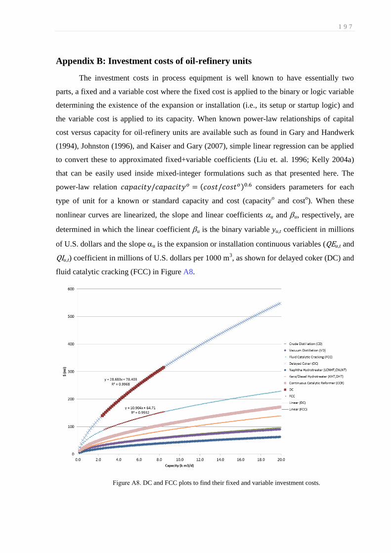
1 9 7

Appendix B: Investment costs of oil-refinery units

The investment costs in process equipment is well known to have essentially two

parts, a fixed and a variable cost where the fixed cost is applied to the binary or logic variable

determining the existence of the expansion or installation (i.e., its setup or startup logic) and

the variable cost is applied to its capacity. When known power-law relationships of capital

cost versus capacity for oil-refinery units are available such as found in Gary and Handwerk

(1994), Johnston (1996), and Kaiser and Gary (2007), simple linear regression can be applied

to convert these to approximated fixed+variable coefficients (Liu et. al. 1996; Kelly 2004a)

that can be easily used inside mixed-integer formulations such as that presented here. The

power-law relation ( ) considers parameters for each

type of unit for a known or standard capacity and cost (capacityo and cost

o). When these

nonlinear curves are linearized, the slope and linear coefficients u and u, respectively, are

determined in which the linear coefficient u is the binary variable yu,t coefficient in millions

of U.S. dollars and the slope u is the expansion or installation continuous variables (QEu,t and

QIu,t) coefficient in millions of U.S. dollars per 1000 m3, as shown for delayed coker (DC) and

fluid catalytic cracking (FCC) in Figure A8.

Figure A8. DC and FCC plots to find their fixed and variable investment costs.

1 9 8

Clearly, the unit investment costs have three distinct regions to be linearized. The

initial between 0.8 and 2.4 m3/d, the intermediate between 2.4 and 9 m

3/d (as represented for

DC and FCC), and the final region for unit with capacity bigger than 9 m3/d. As they need to

be known a priori before the capacity size determination, these parameters or costs can be

updated after each MILP-NLP iteration considering the capacity increment size found the last

MILP problem performed.

1 9 9

Appendix C: IMPL’s configuration and equations formed for the

motivating example 1

i M P l (c)

Copyright and Property of i n d u s t r I A L g o r i t h m s LLC.

!!!!!!!!!!!!!!!!!!!!!!!!!!!!!!!!!!!!!!!!!!!!!!!!!!!!!!!!!!!!!!!!!!!!!!!!!!!!!!!!

! Calculation Data (Parameters)

!!!!!!!!!!!!!!!!!!!!!!!!!!!!!!!!!!!!!!!!!!!!!!!!!!!!!!!!!!!!!!!!!!!!!!!!!!!!!!!!

&sCalc,@sValue

START,-1.0

BEGIN,0.0

END,3.0

PERIOD,1.0

LARGE,10000.0

ALPHA,0.5

BETA,0.5

OLDCAPACITY,1.0

NEWCAPACITY,1.5

&sCalc,@sValue

!!!!!!!!!!!!!!!!!!!!!!!!!!!!!!!!!!!!!!!!!!!!!!!!!!!!!!!!!!!!!!!!!!!!!!!!!!!!!!!!

! Chronological Data (Periods)

!!!!!!!!!!!!!!!!!!!!!!!!!!!!!!!!!!!!!!!!!!!!!!!!!!!!!!!!!!!!!!!!!!!!!!!!!!!!!!!!

@rPastTHD,@rFutureTHD,@rTPD

START,END,PERIOD

@rPastTHD,@rFutureTHD,@rTPD

!!!!!!!!!!!!!!!!!!!!!!!!!!!!!!!!!!!!!!!!!!!!!!!!!!!!!!!!!!!!!!!!!!!!!!!!!!!!!!!!

! Construction Data (Pointers)

!!!!!!!!!!!!!!!!!!!!!!!!!!!!!!!!!!!!!!!!!!!!!!!!!!!!!!!!!!!!!!!!!!!!!!!!!!!!!!!!

&sUnit,&sOperation,@sType,@sSubtype,@sUse

A,,perimeter,,

B,,perimeter,,

Capacity,,pool,,

Capital,Cost,perimeter,,

Charge,,processc,,

Process,Commission,processc,,

Process,Existing,processc,,

Process,Expand,processc,,

&sUnit,&sOperation,@sType,@sSubtype,@sUse

&sUnit,&sOperation,&sPort,&sState,@sType,@sSubtype

A,,a,,out,

B,,b,,in,

Capacity,,i,,in,

2 0 0

Capacity,,o,,out,

Capital,Cost,cpl,,in,

Charge,,cpl,,out,

Charge,,cpt,,out,

Charge,,i,,in,

Process,Commission,a,,in,

Process,Commission,b,,out,

Process,Commission,cpt,,out,

Process,Existing,a,,in,

Process,Existing,b,,out,

Process,Expand,a,,in,

Process,Expand,b,,out,

Process,Expand,cpt,,in,

&sUnit,&sOperation,&sPort,&sState,@sType,@sSubtype

&sUnit,&sOperation,&sPort,&sState,&sUnit,&sOperation,&sPort,&sState

A,,a,,Process,Commission,a,

A,,a,,Process,Existing,a,

A,,a,,Process,Expand,a,

Capacity,,o,,Process,Expand,cpt,

Charge,,cpl,,Capital,Cost,cpl,

Charge,,cpt,,Capacity,,i,

Process,Commission,b,,B,,b,

Process,Commission,cpt,,Charge,,i,

Process,Existing,b,,B,,b,

Process,Expand,b,,B,,b,

&sUnit,&sOperation,&sPort,&sState,&sUnit,&sOperation,&sPort,&sState

!!!!!!!!!!!!!!!!!!!!!!!!!!!!!!!!!!!!!!!!!!!!!!!!!!!!!!!!!!!!!!!!!!!!!!!!!!!!!!!!

! Capacity Data (Prototypes)

!!!!!!!!!!!!!!!!!!!!!!!!!!!!!!!!!!!!!!!!!!!!!!!!!!!!!!!!!!!!!!!!!!!!!!!!!!!!!!!!

&sUnit,&sOperation,@rRate_Lower,@rRate_Upper

Process,Existing,0.0,OLDCAPACITY

Process,Commission,0.0,OLDCAPACITY

Process,Expand,0.0,LARGE

Charge,,0.0,NEWCAPACITY

&sUnit,&sOperation,@rRate_Lower,@rRate_Upper

&sUnit,&sOperation,@rHoldup_Lower,@rHoldup_Upper

Capacity,,0.0,NEWCAPACITY*END

&sUnit,&sOperation,@rHoldup_Lower,@rHoldup_Upper

&sUnit,&sOperation,&sPort,&sState,@rTotalRate_Lower,@rTotalRate_Upper

ALLINPORTS,0.0,LARGE

ALLOUTPORTS,0.0,LARGE

&sUnit,&sOperation,&sPort,&sState,@rTotalRate_Lower,@rTotalRate_Upper

2 0 1

&sUnit,&sOperation,&sPort,&sState,@rTeeRate_Lower,@rTeeRate_Upper

ALLINPORTS,0.0,LARGE

ALLOUTPORTS,0.0,LARGE

Process,Expand,cpt,,0.0,NEWCAPACITY

&sUnit,&sOperation,&sPort,&sState,@rTeeRate_Lower,@rTeeRate_Upper

&sUnit,&sOperation,&sPort,&sState,@rYield_Lower,@rYield_Upper,@rYield_Fixed

Process,Existing,a,,1.0,1.0,

Process,Existing,b,,1.0,1.0,

Process,Commission,a,,1.0,1.0,

Process,Commission,b,,1.0,1.0,

Process,Commission,cpt,,0.0,LARGE,

Process,Expand,a,,1.0,1.0,

Process,Expand,b,,1.0,1.0,

Charge,,i,,1.0,1.0

Charge,,cpl,,ALPHA,ALPHA,BETA-ALPHA*OLDCAPACITY

Charge,,cpt,,0.0,0.0

Process,Expand,cpt,,1.0,LARGE,

&sUnit,&sOperation,&sPort,&sState,@rYield_Lower,@rYield_Upper,@rYield_Fixed

!!!!!!!!!!!!!!!!!!!!!!!!!!!!!!!!!!!!!!!!!!!!!!!!!!!!!!!!!!!!!!!!!!!!!!!!!!!!!!!!

! Constriction Data (Practices/Policies)

!!!!!!!!!!!!!!!!!!!!!!!!!!!!!!!!!!!!!!!!!!!!!!!!!!!!!!!!!!!!!!!!!!!!!!!!!!!!!!!!

&sUnit,&sOperation,@rUpTiming_Lower,@rUpTiming_Upper

Process,Commission,1.0,1.0

Process,Expand,END,

&sUnit,&sOperation,@rUpTiming_Lower,@rUpTiming_Upper

!!!!!!!!!!!!!!!!!!!!!!!!!!!!!!!!!!!!!!!!!!!!!!!!!!!!!!!!!!!!!!!!!!!!!!!!!!!!!!!!

! Consolidation Data (Partitioning)

!!!!!!!!!!!!!!!!!!!!!!!!!!!!!!!!!!!!!!!!!!!!!!!!!!!!!!!!!!!!!!!!!!!!!!!!!!!!!!!!

&sUnit,&sOperation,&sOperationGroup

Process,Existing,ExistingGroup

Process,Expand,ExpandGroup

&sUnit,&sOperation,&sOperationGroup

!!!!!!!!!!!!!!!!!!!!!!!!!!!!!!!!!!!!!!!!!!!!!!!!!!!!!!!!!!!!!!!!!!!!!!!!!!!!!!!!

! Compatibility Data (Phasing, Prohibiting, Purging, Postponing)

!!!!!!!!!!!!!!!!!!!!!!!!!!!!!!!!!!!!!!!!!!!!!!!!!!!!!!!!!!!!!!!!!!!!!!!!!!!!!!!!

&sUnit,&sOperationGroup,&sOperationGroup,@sOperation

Process,ExistingGroup,ExpandGroup,Commission

&sUnit,&sOperationGroup,&sOperationGroup,@sOperation

!!!!!!!!!!!!!!!!!!!!!!!!!!!!!!!!!!!!!!!!!!!!!!!!!!!!!!!!!!!!!!!!!!!!!!!!!!!!!!!!

! Cost Data (Pricing)

!!!!!!!!!!!!!!!!!!!!!!!!!!!!!!!!!!!!!!!!!!!!!!!!!!!!!!!!!!!!!!!!!!!!!!!!!!!!!!!!

&sUnit,&sOperation,&sPort,&sState,@rFlowPro_Weight,@rFlowPer1_Weight,@rFlowPer2_Weight,@rFlowPen_Weight

2 0 2

A,,a,,0.0

B,,b,,1.0

Capital,Cost,cpl,,-1.0

&sUnit,&sOperation,&sPort,&sState,@rFlowPro_Weight,@rFlowPer1_Weight,@rFlowPer2_Weight,@rFlowPen_Weight

!!!!!!!!!!!!!!!!!!!!!!!!!!!!!!!!!!!!!!!!!!!!!!!!!!!!!!!!!!!!!!!!!!!!!!!!!!!!!!!!

! Content Data (Past, Present Provisos)

!!!!!!!!!!!!!!!!!!!!!!!!!!!!!!!!!!!!!!!!!!!!!!!!!!!!!!!!!!!!!!!!!!!!!!!!!!!!!!!!

&sUnit,&sOperation,@rHoldup_Value,@rStart_Time

Capacity,,0.0,0.0

&sUnit,&sOperation,@rHoldup_Value,@rStart_Time

&sUnit,&sOperation,@rSetup_Value,@rStart_Time

Process,Existing,1,START

&sUnit,&sOperation,@rSetup_Value,@rStart_Time

!!!!!!!!!!!!!!!!!!!!!!!!!!!!!!!!!!!!!!!!!!!!!!!!!!!!!!!!!!!!!!!!!!!!!!!!!!!!!!!!

! Command Data (Future Provisos)

!!!!!!!!!!!!!!!!!!!!!!!!!!!!!!!!!!!!!!!!!!!!!!!!!!!!!!!!!!!!!!!!!!!!!!!!!!!!!!!!

&sUnit,&sOperation,@rSetup_Lower,@rSetup_Upper,@rBegin_Time,@rEnd_Time

ALLPARTS,0,1,BEGIN,END

&sUnit,&sOperation,@rSetup_Lower,@rSetup_Upper,@rBegin_Time,@rEnd_Time

&sUnit,&sOperation,&sPort,&sState,&sUnit,&sOperation,&sPort,&sState,@rSetup_Lower,@rSetup_Upper,@rBegin_Time,@rEnd_Time

ALLPATHS,0,1,BEGIN,END

&sUnit,&sOperation,&sPort,&sState,&sUnit,&sOperation,&sPort,&sState,@rSetup_Lower,@rSetup_Upper,@rBegin_Time,@rEnd_Time

&sUnit,&sOperation,&sPort,&sState,@rYield_Lower,@rYield_Upper,@rYield_Target,@rBegin_Time,@rEnd_Time

Charge,,cpt,,1.0*(END-1.0),1.0*(END-1.0),,0.0,1.0



&sUnit,&sOperation,&sPort,&sState,@rYield_Lower,@rYield_Upper,@rYield_Target,@rBegin_Time,@rEnd_Time

Index Names:

1..U: units.

1..M: unit-operations.

1..I: unit-operation-port-states (in).

1..J: unit-operation-port-states (out).

1..SG: unit-operation sequence-groups.

1..NTPF: time-periods in both the past and future time-horizons.

1..NTF: time-periods in both the future time-horizon.

Variable Names:

v2r_ymsu(1..M,1..NTPF): unit-operation (M) setup variable.

v3r_yjisu(1..J,1..I,1..NTPF): unit-operation-port-state-unit-operation-port-state (JI) setup variable.

v2r_xmf(1..M,1..NTPF): unit-operation (M) flow variable.

v2r_xmh(1..M,1..NTPF): unit-operation (M) holdup variable.

v3r_xjif(1..J,1..I,1..NTPF): unit-operation-port-state-unit-operation-port-state (JI) flow variable.

2 0 3

v2r_zmsu(1..M,1..NTPF): unit-operation (M) startup variable.

v2r_zmsv(1..M,1..NTPF): unit-operation (M) switchover-to-itself variable.

v2r_zmsd(1..M,1..NTPF): unit-operation (M) shutdown variable.

v2r_zysgsu(1..SG,1..NTF): unit-operation sequence-group (SG) memory setup variable.

Constraint Names:

c2r_xmflower(1..M,1..NTF): unit-operation (M) flow lower semi-continuous constraint.

c2r_xmfupper(1..M,1..NTF): unit-operation (M) flow upper semi-continuous constraint.

c3r_xjifupper(1..J,1..I,1..NTF): unit-operation-port-state-unit-operation-port-state (JI) upper flow constraint.

c2r_xjyupper(1..J,1..NTF): unit-operation-port-state (J) upper yield constraint.

c2r_xuhbalance(1..U,1..NTF): unit (U) holdup balance constraint.

c2r_yumultiuseupper(1..U,1..NTF): unit (U) upper multi-use setup constraint.

c2r_yumultiusesos1(1..U,1..NTF): unit (U) multi-use setup special-order-set-one (SOS1).

c3r_yjistructuraltrans(1..J,1..I,1..NTF): unit-operation-port-state-unit-operation-port-state (JI) structural transition

constraint.

c2r_zmsutemporaltrans(1..M,1..NTF): unit-operation (M) setup temporal transition constraint.

c2r_zmsdtemporaltrans(1..M,1..NTF): unit-operation (M) shutdown temporal transition constraint.

c2r_zmsvtemporaltrans(1..M,1..NTF): unit-operation (M) switchover-to-itself temporal transition constraint.

c2r_zmsvtemporaltranssos1(1..M,1..NTF): unit-operation (M) switch-over-to-itself temporal transition special-ordered-set-one

(SOS1).

c2r_ymuptimelower(1..M,1..NTF): unit-operation (M) lower uptime constraint.

c2r_ymuptimeupper(1..M,1..NTF): unit-operation (M) upper uptime constraint.

c2r_ymuptime(1..M,1..NTF): unit-operation (M) uptime temporal aggregation cut constraint.

c2r_zyusingleuse(1..U,1..NTF): unit (U) memory setup single-use constraint.

c2r_zyusingleusesos1(1..U,1..NTF): unit (U) memory setup single-use special-ordered-set-one (sos1).

c2r_zysgsu1(1..SG,1..NTF): unit-operation sequence-group (SG) memory setup constraint one.

c2r_zysgsu2(1..SG,1..NTF): unit-operation sequence-group (SG) memory setup constraint two.

c3r_zsgswseqdeptemporal3(1..SG,1..SG,1..NTF): unit-operation sequence-group (SG) switchover-to-others sequence-dependent

temporal constraint three.

c1_gprofitterm(1): profit term constraint.

c1_totalobjfun(1): total objective function constraint.

Constraints and Bounds:

c2r_xmflower(5,1) <= 1.000000000000000E-004 v2r_ymsu(5,1) -1 v2r_xmf(5,1)



c2r_xmfupper(7,1) <= 1 v2r_xmf(7,1) -1 v2r_ymsu(7,1)









2 0 4

c2r_xmfupper(5,1) <= 1 v2r_xmf(5,1) -1.50000000000000 v2r_ymsu(5,1)



c2r_xifupper(1,1) <= 1 v3r_xjif(5,1,1) 1 v3r_xjif(7,1,1) 1 v3r_xjif(8,1,1) -10000 v2r_ymsu(2,1)



c2r_xifupper(3,1) <= 1 v3r_xjif(3,3,1) -10000 v2r_ymsu(4,1)



c2r_xjfupper(1,1) <= 1 v3r_xjif(1,5,1) 1 v3r_xjif(1,6,1) 1 v3r_xjif(1,7,1) -10000 v2r_ymsu(1,1)



c3r_xjifupper(1,5,1) <= 1 v3r_xjif(1,5,1) -10000 v3r_yjisu(1,5,1)









c3r_xjifupper(2,8,1) <= 1 v3r_xjif(2,8,1) -1.50000000000000 v3r_yjisu(2,8,1)




















c2r_xiylower(4,1) = 1 v2r_xmf(5,1) -1 v3r_xjif(6,4,1)

2 0 5












c2r_xiylower(8,1) <= 1 v2r_xmf(8,1) -1 v3r_xjif(2,8,1)



c2r_xiyupper(8,1) <= 1 v3r_xjif(2,8,1) -10000 v2r_xmf(8,1)



c2r_xjylower(3,1) = 0.500000000000000 v2r_xmf(5,1) -1 v3r_xjif(3,3,1)



c2r_xjylower(4,1) = 2 v2r_xmf(5,1) -1 v3r_xjif(4,2,1)











c2r_xjyupper(6,1) <= 1 v3r_xjif(6,4,1) -10000 v2r_xmf(6,1)



c2r_xuhbalance(3,1) = -1 v2r_xmh(3,1) 1 v3r_xjif(4,2,1) -1 v3r_xjif(2,8,1)

c2r_xuhbalance(3,2) = 1 v2r_xmh(3,1) -1 v2r_xmh(3,2) 1 v3r_xjif(4,2,2) -1 v3r_xjif(2,8,2)

c2r_xuhbalance(3,3) = 1 v2r_xmh(3,2) -1 v2r_xmh(3,3) -1 v3r_xjif(2,8,3)

c2r_yumultiuseupper(6,1) <= 1 v2r_ymsu(6,1) 1 v2r_ymsu(7,1) 1 v2r_ymsu(8,1) -1.000000000000000



c2r_yumultiusesos1(6,1) 1 v2r_ymsu(6,1) 2 v2r_ymsu(7,1) 3 v2r_ymsu(8,1)


2 0 6


c3r_yjistructuraltrans(1,5,1) <= 2 v3r_yjisu(1,5,1) -1 v2r_ymsu(1,1) -1 v2r_ymsu(6,1)









c3r_yjistructuraltrans(2,8,1) <= 2 v3r_yjisu(2,8,1) -1 v2r_ymsu(8,1) -1.000000000000000





















c2r_zmsutemporaltrans(6,1) = 1 v2r_ymsu(6,1) -1 v2r_zmsu(6,1) 1 v2r_zmsd(6,1)

c2r_zmsutemporaltrans(6,2) = 1 v2r_ymsu(6,2) -1 v2r_ymsu(6,1) -1 v2r_zmsu(6,2) 1 v2r_zmsd(6,2)


c2r_zmsutemporaltrans(8,1) = 1 v2r_ymsu(8,1) -1 v2r_zmsu(8,1) 1 v2r_zmsd(8,1)



c2r_zmsdtemporaltrans(6,1) = 1 v2r_ymsu(6,1) -1 v2r_zmsu(6,1) -1 v2r_zmsd(6,1) -2 v2r_zmsv(6,1)

c2r_zmsdtemporaltrans(6,2) = 1 v2r_ymsu(6,2) 1 v2r_ymsu(6,1) -1 v2r_zmsu(6,2) -1 v2r_zmsd(6,2)

-2 v2r_zmsv(6,2)


-2 v2r_zmsv(6,3)

2 0 7

c2r_zmsdtemporaltrans(8,1) = 1 v2r_ymsu(8,1) -1 v2r_zmsu(8,1) -1 v2r_zmsd(8,1) -2 v2r_zmsv(8,1)


-2 v2r_zmsv(8,2)


-2 v2r_zmsv(8,3)

c2r_zmsvtemporaltrans(6,1) <= 1 v2r_zmsu(6,1) 1 v2r_zmsd(6,1) 1 v2r_zmsv(6,1) -1.000000000000000






c2r_zmsvtemporaltranssos1(6,1) 1 v2r_zmsu(6,1) 2 v2r_zmsd(6,1) 3 v2r_zmsv(6,1)






c2r_ymuptimelower(8,2) <= 1 v2r_zmsu(8,1) -1 v2r_ymsu(8,2)

c2r_ymuptimelower(8,3) <= 1 v2r_zmsu(8,2) 1 v2r_zmsu(8,1) -1 v2r_ymsu(8,3)

c2r_ymuptimeupper(6,1) <= 1 v2r_ymsu(6,1) 1 v2r_ymsu(6,2) 1 v2r_ymsu(6,3) -2.00000000000000

c1_ymuptime(8,1) <= 3 v2r_zmsu(8,1) 3 v2r_zmsu(8,2) 3 v2r_zmsu(8,3) -3.00000000000000

c2r_zyusingleuse(6,1) = 1 v2r_zysgsu(1,1) 1 v2r_zysgsu(2,1) -1.000000000000000



c2r_zyusingleusesos1(6,1) 1 v2r_zysgsu(1,1) 2 v2r_zysgsu(2,1)



c2r_zysgsu1(1,1) <= 1 v2r_ymsu(7,1) -1 v2r_zysgsu(1,1)






c2r_zysgsu2(1,2) <= 1 v2r_zysgsu(1,2) -1 v2r_zysgsu(1,1)

c2r_zysgsu2(1,3) <= 1 v2r_zysgsu(1,3) -1 v2r_zysgsu(1,2)

c2r_zysgsu2(2,1) <= 1 v2r_zysgsu(2,1) -1 v2r_zmsu(8,1)

c2r_zysgsu2(2,2) <= 1 v2r_zysgsu(2,2) -1 v2r_zysgsu(2,1) -1 v2r_zmsu(8,2)

c2r_zysgsu2(2,3) <= 1 v2r_zysgsu(2,3) -1 v2r_zysgsu(2,2) -1 v2r_zmsu(8,3)

c3r_zsgswseqdeptemporal3(1,2,1) <= 1 v2r_zysgsu(2,1) 1 v2r_zmsu(8,1) -1 v2r_zmsd(6,1) -1.000000000000000

c3r_zsgswseqdeptemporal3(1,2,2) <= 1 v2r_zysgsu(2,2) 1 v2r_zysgsu(1,1) 1 v2r_zmsu(8,2)

-1 v2r_zmsd(6,2) -2.00000000000000

c3r_zsgswseqdeptemporal3(1,2,3) <= 1 v2r_zysgsu(2,3) 1 v2r_zysgsu(1,2) 1 v2r_zmsu(8,3)

2 0 8

-1 v2r_zmsd(6,3) -2.00000000000000

c1_gprofitterm(1,1) = 1 v1_gprofitterm(1,1) 1 v3r_xjif(3,3,1) 1 v3r_xjif(3,3,2)

1 v3r_xjif(3,3,3) -1 v3r_xjif(5,1,1) -1 v3r_xjif(5,1,2) -1 v3r_xjif(5,1,3) -1 v3r_xjif(7,1,1)

-1 v3r_xjif(7,1,2) -1 v3r_xjif(7,1,3) -1 v3r_xjif(8,1,1) -1 v3r_xjif(8,1,2) -1 v3r_xjif(8,1,3)

c1_totalobjfun(5,1) = 1 v1_totalobjfun(5,1) -1 v1_gprofitterm(1,1)

0 <= v2r_ymsu(1,1) <= 1

0 <= v2r_ymsu(1,2) <= 1

0 <= v2r_ymsu(1,3) <= 1

0 <= v2r_ymsu(2,1) <= 1

0 <= v2r_ymsu(2,2) <= 1

0 <= v2r_ymsu(2,3) <= 1

0 <= v2r_ymsu(4,1) <= 1

0 <= v2r_ymsu(4,2) <= 1

0 <= v2r_ymsu(4,3) <= 1

0 <= v2r_ymsu(5,1) <= 1

0 <= v2r_ymsu(5,2) <= 1

0 <= v2r_ymsu(5,3) <= 1

0 <= v2r_ymsu(6,1) <= 1

0 <= v2r_ymsu(6,2) <= 1

0 <= v2r_ymsu(6,3) <= 1

0 <= v2r_ymsu(7,1) <= 1

0 <= v2r_ymsu(7,2) <= 1

0 <= v2r_ymsu(7,3) <= 1

0 <= v2r_ymsu(8,1) <= 1

0 <= v2r_ymsu(8,2) <= 1

0 <= v2r_ymsu(8,3) <= 1

0 <= v3r_yjisu(1,5,1) <= 1

0 <= v3r_yjisu(1,5,2) <= 1

0 <= v3r_yjisu(1,5,3) <= 1

0 <= v3r_yjisu(1,6,1) <= 1

0 <= v3r_yjisu(1,6,2) <= 1

0 <= v3r_yjisu(1,6,3) <= 1

0 <= v3r_yjisu(1,7,1) <= 1

0 <= v3r_yjisu(1,7,2) <= 1

0 <= v3r_yjisu(1,7,3) <= 1

0 <= v3r_yjisu(2,8,1) <= 1

0 <= v3r_yjisu(2,8,2) <= 1

0 <= v3r_yjisu(2,8,3) <= 1

0 <= v3r_yjisu(3,3,1) <= 1

0 <= v3r_yjisu(3,3,2) <= 1

0 <= v3r_yjisu(3,3,3) <= 1

2 0 9

0 <= v3r_yjisu(4,2,1) <= 1

0 <= v3r_yjisu(4,2,2) <= 1

0 <= v3r_yjisu(4,2,3) <= 1

0 <= v3r_yjisu(5,1,1) <= 1

0 <= v3r_yjisu(5,1,2) <= 1

0 <= v3r_yjisu(5,1,3) <= 1

0 <= v3r_yjisu(6,4,1) <= 1

0 <= v3r_yjisu(6,4,2) <= 1

0 <= v3r_yjisu(6,4,3) <= 1

0 <= v3r_yjisu(7,1,1) <= 1

0 <= v3r_yjisu(7,1,2) <= 1

0 <= v3r_yjisu(7,1,3) <= 1

0 <= v3r_yjisu(8,1,1) <= 1

0 <= v3r_yjisu(8,1,2) <= 1

0 <= v3r_yjisu(8,1,3) <= 1

0 <= v2r_xmf(7,1) <= 1

0 <= v2r_xmf(7,2) <= 1

0 <= v2r_xmf(7,3) <= 1

0 <= v2r_xmf(6,1) <= 1

0 <= v2r_xmf(6,2) <= 1

0 <= v2r_xmf(6,3) <= 1

0 <= v2r_xmf(8,1) <= 1.50000000000000

0 <= v2r_xmf(8,2) <= 1.50000000000000

0 <= v2r_xmf(8,3) <= 1.50000000000000

0 <= v2r_xmf(5,1) <= 1.50000000000000

0 <= v2r_xmf(5,2) <= 1.50000000000000

0 <= v2r_xmf(5,3) <= 1.50000000000000

0 <= v2r_xmh(3,1) <= 3

0 <= v2r_xmh(3,2) <= 4.50000000000000

0 <= v2r_xmh(3,3) <= 4.50000000000000

0 <= v3r_xjif(1,5,1) <= 1

0 <= v3r_xjif(1,5,2) <= 1

0 <= v3r_xjif(1,5,3) <= 1

0 <= v3r_xjif(1,6,1) <= 1

0 <= v3r_xjif(1,6,2) <= 1

0 <= v3r_xjif(1,6,3) <= 1

0 <= v3r_xjif(1,7,1) <= 1.50000000000000

0 <= v3r_xjif(1,7,2) <= 1.50000000000000

0 <= v3r_xjif(1,7,3) <= 1.50000000000000

0 <= v3r_xjif(2,8,1) <= 1.50000000000000

0 <= v3r_xjif(2,8,2) <= 1.50000000000000

0 <= v3r_xjif(2,8,3) <= 1.50000000000000

2 1 0

0 <= v3r_xjif(3,3,1) <= 0.750000000000000

0 <= v3r_xjif(3,3,2) <= 0.750000000000000

0 <= v3r_xjif(3,3,3) <= 0.750000000000000

0 <= v3r_xjif(4,2,1) <= 3

0 <= v3r_xjif(4,2,2) <= 1.50000000000000

0 <= v3r_xjif(5,1,1) <= 1

0 <= v3r_xjif(5,1,2) <= 1

0 <= v3r_xjif(5,1,3) <= 1

0 <= v3r_xjif(6,4,1) <= 1.50000000000000

0 <= v3r_xjif(6,4,2) <= 1.50000000000000

0 <= v3r_xjif(6,4,3) <= 1.50000000000000

0 <= v3r_xjif(7,1,1) <= 1

0 <= v3r_xjif(7,1,2) <= 1

0 <= v3r_xjif(7,1,3) <= 1

0 <= v3r_xjif(8,1,1) <= 1.50000000000000

0 <= v3r_xjif(8,1,2) <= 1.50000000000000

0 <= v3r_xjif(8,1,3) <= 1.50000000000000

0 <= v2r_zmsu(6,1) <= 1

0 <= v2r_zmsu(6,2) <= 1

0 <= v2r_zmsu(6,3) <= 1

0 <= v2r_zmsu(8,1) <= 1

0 <= v2r_zmsu(8,2) <= 1

0 <= v2r_zmsu(8,3) <= 1

0 <= v2r_zmsv(6,1) <= 0.500000000000000

0 <= v2r_zmsv(6,2) <= 1

0 <= v2r_zmsv(6,3) <= 1

0 <= v2r_zmsv(8,1) <= 0.500000000000000

0 <= v2r_zmsv(8,2) <= 1

0 <= v2r_zmsv(8,3) <= 1

0 <= v2r_zmsd(6,1) <= 1

0 <= v2r_zmsd(6,2) <= 1

0 <= v2r_zmsd(6,3) <= 1

0 <= v2r_zmsd(8,1) <= 1

0 <= v2r_zmsd(8,2) <= 1

0 <= v2r_zmsd(8,3) <= 1

0 <= v2r_zysgsu(1,1) <= 1

0 <= v2r_zysgsu(1,2) <= 1

0 <= v2r_zysgsu(1,3) <= 1

0 <= v2r_zysgsu(2,1) <= 1

0 <= v2r_zysgsu(2,2) <= 1

0 <= v2r_zysgsu(2,3) <= 1

-1.000000000000000E+020 <= v1_gprofitterm(1,1) <= 1.000000000000000E+020

2 1 1

-1.000000000000000E+020 <= v1_totalobjfun(5,1) <= 1.000000000000000E+020

2 1 2

Appendix D: Net Present Value Formulation for Investment of Oil-Refinery

Units

Net present value (NPV) is the main objective to predict capacity increment of process

units in investment or facilities planning analysis. This is a virtual value meaning how present

decisions can be evaluated regarding future perspectives around possible revenues. In

mathematical programming model, rather than simply production frameworks simulation,

high performance NPV calculation is based on mixed-integer models to install new units or

expand existing ones creating a combinatorial tree to be explored in an optimization

environment to obtain better results. Considerations over work capital, depreciation, and

salvage value must be included in the NPV cost coefficients because it can affect company’s

decisions. The first is the demanded capital to maintain the production, and the second and

third are related to investment cost discounts.

Besides NPV calculation, the company's profitability is also an important investment

qualifier configuring as a quick and easy way to judge the overall production performance.

However, the profit evaluated from the operational gains not actually reflect the income

acquired with the present investment decisions as expected in a strategic decision-making

model for a long-term period, even more dealing with assets like in the oil-refining industry,

in which revamp and installation investments can reach billions of dollars. In real,

operational, investments and financial activities determine the cash in and out to be

considered for the projects evaluations in an accounting perspective formulation as proposed

here.

The cash generation source is the operational gains with the current and possible future

assets. On the other hand, cash outflows can be separated in project investments and work

capital expenditures. The capital investment CI expenses in the projects are compound by

construction, property, equipment, labor, detailed project, investment securities, etc. The work

capital WC guarantees the company's earnings maintenance, affording sufficient cash to cover

ongoing debits. In general WC is supposed to be proportional to CI. In this work

WC=0.0517CI.

Financial transactions can also be included in the cash flow. Continuously the

companies’ borrows, debits, and equity can influence the cash flow, but financial transitions

are not being considered here. Amortization, also not included in the model, is the deduction

with specific expenses over a time period, for example, non-drilling costs sustained while

2 1 3

developing the reserves. Expenses with wells from developed reserves should be amortized,

because by definition, those are the reserves that will be produced as a result of the costs

already incurred. The remaining proved reserves but still underdeveloped are excluded

(Wright and Gallun, 2008).

NPV is evaluated accordingly applicable rules (depreciation), legislation (taxes),

market expectative, monetary policy, company’s specifics, etc. (Guillén et al., 2005). In

general, this is the main objective in a strategic planning model and evaluates the capital

amount gained at the moment of decision in having or not a project. So that a discrete, binary,

or setup variable should be included in an investment model to predict the overall capacity

planning for the oil-refinery units as we propose. NPV is an open formula calculated as the

summation of the cash flows balance in each time interval CFt like in Equation A1.

∑

( )

( )

As proposed here, the time horizon is divided in investment t and operational to time

periods. The NLP operational model calculates the daily profit to be extended to annual gains.

Only after the project execution the productive scenario is modified within the following time

periods recalculating the operational profit. The operational cash flow along the time is

corrected annually by the factor Copto to reflect the deflation suffered by the future annual

gains when it is considered at the present as shown in Equation A2. The interest rate ir

considered is fixed in 10% for the Brazilian market (Trading Economics, 2013).

( ) ( )

The investments expenses when evaluated at once at the moment of decision lessen by

equipment depreciation DEP and salvage value SV deductions. SV is the equipment realized

selling price at the end of its useful life. The value is used to determine depreciation amounts

to deduct taxes. Depreciation in an accounting problem is considered the costs to maintain the

unit production in compliance with safety requirements along its useful lifetime. Usually the

depreciation method is set by the company’s policy and should be in accordance with

regulatory bodies about how and when the deduction may be taken based on what the asset is

and how long it will last. Typically after 25 years, various studies need to be done to

determine options for extending a refining unit useful life, reaching its final salvage value. So,

2 1 4

considering the equipment realized value components as discussed, the investment costs for

each discrete decision to approve the projects are defined in Equation A3.

[ ] ( )

CIt is the liquid cash or project capital investment clamed to build the asset. WCt is the

work capital demanded to maintain the company’s activities. After the total time period

considered for the NPV calculation, the WCt is withdrawn. Deductions from depreciation

DEPt and salvage value SVt reflect the projects no-cash weight to be included in the discrete

variable decision.

To evaluate the realized investment costs along the NPV investigation time Cinvt,

Equations A4 and A5 are needed to find the investment costs deductions related to the WC

cash back, the depreciation tax refunds, and the salvage amount recovered. The model uses

the initial point and the interval of a project execution to determine the economical evaluation

of an asset. Tcurt is the investment time begging in which the discrete decisions are made. The

project execution interval Tt can vary for each unit, but by the sake of simplicity all units

have the same project execution, but the model is ready for different investment intervals.

∑ ( )

∑ ( )

As the model allows investment decision in a multiperiod formulation the costs for the

units to be invested in each t considering their NPV are given by Equation A6. The direct

costs represent the project and work capital expenditures. The work capital factor WCF is a

percentage of the project capital. This cash is ultimately given back at the investment end time

tend. The depreciation deduction is a linear tax refund ratio based on the difference between

the capital to be invested in the equipment and its final salvage value. For oil-refinery units

the useful lifetime considered is tdep = 25 years. Finally the cash gained with the possible

equipment selling is calculated taking in account the salvage value factor (SVF) which is

considered 5% for all units. It means that after 25 years the value for a unit is 5% of its startup

value. The startup value considered here is the CIt for a unit deflated by the interval to have it

2 1 5

built. Also the deflation is applied when the non-cash inflows are return to the present. Only

after the projects execution intervals Tt the depreciation refunds and salvage value can be

applied.

( ) (

( )

( ) )

( ( )

)( )

∑

( )

(

)

( ) ( )

For future projects starting in further intervals, the liquid cash granted at the moment

of decision should return to the present deflating as shown in the equation (S6) for the CI and

the WC expenses. The CI and WC amounts defined for the projects in the first period are

withdrawn at the moment of decision, so that the interest rate correction is not applied

(Tcur1=0) . As mentioned, the WC is rescued at the portfolio evaluation end time reducing the

overall project costs. The other non-cash deductions are related with the equipment existence

along the time. The liquid cash invested in a project is converted in the current asset which

during its life demands capital to maintain its integrity and safety. This expense is discounted

as a tax refund so-called depreciation (DEP). As the refunds are collected within the total

investment period in evaluation tend, maybe shorter than the useful lifetime, the depreciation

discount is deflated at every year after the unit startup until tend. An annual straight-line

depreciation ratio determines the total amount refund for each project until the final time

studied by the investment portfolio investigation. Finally, the last term in equation (S6) is

related with the current salvage value (SV) held by the equipment built. As like for

depreciation, an annual linear reduction along the unit useful lifetime compute the amount lost

after its startup, but its deflation is accounted only at the end time period when its current SV

is realized at the moment of decision.

2 1 6

Supporting Information

Table S3.1. Crude-oil assay yields, Ycr,c (%).

Table S3.2. Crude-oil assay specific gravity, Gcr,c (g/cm3).

Table S3.3. Crude-oil assay sulfur content, Scr,c (w%).

Table S3.4. Crude-oil assay acidity, Acr,c (mgKOH/g).

C1C2 C3C4 N SW1 K SW2 LD SW3 HD ATR LVGO HVGO VR

National Light 0.01 1.06 6.72 4.85 13.64 11.91 17.38 9.17 7.78 27.48 18.81 2.38 6.30

Pre-Salt 0.09 1.02 8.72 5.02 6.89 5.55 6.91 4.24 4.46 57.11 21.81 5.30 29.99

Medium 0.12 0.90 7.20 3.50 6.30 5.58 7.34 4.71 4.78 59.58 20.96 5.41 33.20

Heavy 0.08 0.44 4.50 2.05 4.46 5.10 9.20 6.11 5.77 62.28 19.71 4.97 37.61

Imported Ultra Light 0.06 3.38 19.82 8.86 12.35 9.87 12.57 7.40 6.25 19.43 13.59 1.51 4.34

Crude

Crude N SW1 K SW2 LD SW3 HD ATR LVGO HVGO VR

National Light 0.722 0.779 0.806 0.843 0.861 0.868 0.880 0.936 0.916 0.948 0.994

Pre-Salt 0.701 0.753 0.789 0.819 0.840 0.853 0.867 0.944 0.903 0.935 0.976

Medium 0.698 0.763 0.798 0.829 0.850 0.865 0.883 0.969 0.920 0.944 1.004

Heavy 0.726 0.776 0.804 0.832 0.860 0.882 0.906 0.986 0.940 0.956 1.015

Imported Ultra Light 0.713 0.756 0.780 0.804 0.823 0.833 0.845 0.916 0.886 0.937 1.004


National Light 0.001 0.007 0.017 0.032 0.056 0.081 0.109 0.196 0.150 0.208 0.316

Pre-Salt 0.032 0.037 0.056 0.076 0.112 0.175 0.227 0.501 0.312 0.423 0.642

Medium 0.001 0.007 0.045 0.093 0.187 0.325 0.372 0.723 0.539 0.613 0.855

Heavy 0.002 0.025 0.105 0.232 0.400 0.503 0.638 0.746 0.676 0.709 0.785



National Light 0.010 0.036 0.060 0.066 0.072 0.095 0.188 0.573 0.588 0.543 0.543

Pre-Salt 0.124 0.118 0.168 0.207 0.270 0.293 0.266 0.291 0.250 0.227 0.329

Medium 0.026 0.030 0.053 0.111 0.250 0.378 0.532 0.196 0.362 0.294 0.084

Heavy 0.015 0.033 0.054 0.133 0.339 0.776 1.432 1.276 1.743 1.696 0.997


2 1 7

Table S3.5. Products yields and properties for other oil-refinery units.

Table S3.6. Parameter for RON and MON blend values.

Unit (u) Stream (s) Yu,s (%) Gu,s (g/cm3) Su,s (w%) MONu,s RONu,s AROu,s OLEu,s

RFCC C1C2 5

C3C4 11

LCN 54 0.758 0.098 80.00 92.00 45.00 29.00

HCN 5 0.857 0.120

LCO 7 0.901 0.343

DO 18 0.956 0.453

FCC C1C2 4

C3C4 10

LCN 54 0.758 0.098 81.78 94.05 45.00 29.00

HCN 7 0.857 0.120

LCO 10 0.901 0.343

DO 15 0.956 0.453

HCC C1C2 3

C3C4 7

HCCN 15 0.758 0.001 69.00 76.00 2.00 1.00

HCCK 18 0.770 0.001

HCCD 25 0.850 0.001

HCCO 32 0.900 0.001

PDA DAO 54 0.929 0.748

ASFR 46 1.090 0.857

DC C1C2 4

C3C4 8

CLN 15 0.750 0.427 65.88 68.96 10.69 4.00

CHN 12 0.786 0.537

CLGO 12 0.845 0.597

CMGO 8 0.925 0.679

CHGO 13 0.967 0.759

COKE 28

KHT HTK 100 GKHT SKHT

D1HT HTD 98 GD1HT SD1HT

D2HT HTD 96 GD2HT SD2HT

LCNHT HTLCN 100 GLCNHT SLCNHT MONLCNHT RONLCNHT AROLCNHT OLELCNHT

CLNHT HTCLN 100 GCLNHT SCLNHT MONCLNHT RONCLNHT AROCLNHT OLECLNHT

ST LNST 40 0.710 SCLNHT 65.0 75.0

HNST 50 0.790 SCLNHT 65.0 75.0

GOST 10 0.855 SCLNHT

REF H2 12

REFOR 88 0.850 0.005 92.00 100.00 50.00 1.00

ETHimp ETH 100 0.789 0.000 90.00 109.00

GLNimp GIMP 100 0.758 0.005 81.78 94.05 20.00 5.00

JETimp KIMP 100 0.800 0.030

LSDimp DIMP 100 0.830 0.001

Parameter

RON a 0.01929

b 0.00043

c 0.00144

d 0.00165

MON e 0.04450

f 0.00081

g 0.000000645

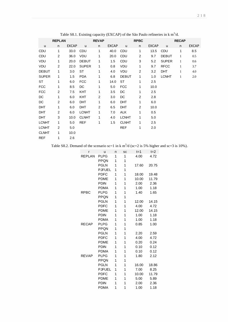
2 1 8

Table S8.1. Existing capacity (EXCAP) of the São Paulo refineries in k m3/d.

Table S8.2. Demand of the scenario sc=1 in k m3/d (sc=2 is 5% higher and sc=3 is 10%).

REPLAN REVAP RPBC RECAP

u n EXCAP u n EXCAP u n EXCAP u n EXCAP

CDU 1 33.0 CDU 1 40.0 CDU 1 13.5 CDU 1 8.5

CDU 2 36.0 VDU 1 20.0 CDU 2 9.7 DEBUT 1 0.5

VDU 1 20.0 DEBUT 1 1.5 CDU 3 5.2 SUPER 1 0.6

VDU 2 22.0 SUPER 1 0.8 VDU 1 9.7 RFCC 1 3.7

DEBUT 1 3.0 ST 1 4.0 VDU 2 3.2 DHT 1 4.0

SUPER 1 1.5 PDA 1 6.8 DEBUT 1 1.0 LCNHT 1 2.0

ST 1 6.0 FCC 1 14.0 ST 1 2.5

FCC 1 8.5 DC 1 5.0 FCC 1 10.0

FCC 2 7.5 KHT 1 3.5 DC 1 2.5

DC 1 6.0 KHT 2 3.0 DC 2 2.8

DC 2 6.0 DHT 1 6.0 DHT 1 6.0

DHT 1 6.0 DHT 2 6.5 DHT 2 10.0

DHT 2 6.0 LCNHT 1 7.0 ALK 1 0.5

DHT 3 10.0 CLNHT 1 4.0 LCNHT 1 5.0

LCNHT 1 5.0 REF 1 1.5 CLNHT 1 2.5

LCNHT 2 5.0 REF 1 2.0

CLNHT 1 10.0

REF 1 2.6

r u n sc t=1 t=2

REPLAN PLPG 1 1 4.00 4.72

PPQN 1 1

PGLN 1 1 17.60 20.75

PJFUEL 1 1

PDFC 1 1 18.00 19.48

PDME 1 1 10.00 11.79

PDIN 1 1 2.00 2.36

PDMA 1 1 1.00 1.18

RPBC PLPG 1 1 1.40 1.65

PPQN 1 1

PGLN 1 1 12.00 14.15

PDFC 1 1 4.00 4.72

PDME 1 1 12.00 14.15

PDIN 1 1 1.00 1.18

PDMA 1 1 1.00 1.18

RECAP PLPG 1 1 0.85 1.00

PPQN 1 1

PGLN 1 1 2.20 2.59

PDFC 1 1 4.00 4.72

PDME 1 1 0.20 0.24

PDIN 1 1 0.10 0.12

PDMA 1 1 0.10 0.12

REVAP PLPG 1 1 1.80 2.12

PPQN 1 1

PGLN 1 1 16.00 18.86

PJFUEL 1 1 7.00 8.25

PDFC 1 1 10.00 11.79

PDME 1 1 5.00 5.89

PDIN 1 1 2.00 2.36

PDMA 1 1 1.00 1.18

2 1 9

References

[1] Agencia T1. Preço de querosene de aviação ainda pesa nas passagens aéreas Home Page.

http://www.agenciat1.com.br/preco-de-querosene-de-aviacao-ainda-pesa-nas-passagens-

areas (Access Apr 30, 2013).

[2] Alattas, A.M.; Grossmann, I.E.; Palou-Rivera, I. Integration of Nonlinear Crude

Distillation Unit Models in Refinery Planning Optimization. Industrial & Engineering

Chemistry Research, 50, 6860-6870, 2011.

[3] Alattas, A.M.; Grossmann, I.E.; Palou-Rivera, I. Refinery Production Planning-

Multiperiod MINLP with Nonlinear CDU Model. Industrial & Engineering Chemistry

Research, 2012, 50, 6860-6870, 2012.

[4] ANP Petroleum National Agency. Brazilian Annual Oil Statistic 2012 Home Page.

http://www.anp.gov.br/?pg=62463&m=&t1=&t2=&t3=&t4=&ar=&ps=&cachebust=1371

79937518 (Access Nov 30, 2013).

[5] ANP Petroleum National Agency. uels and Derivatives Mar et Evolution 2 -2 12.

Available on line at www.anp.gov.br dw 6 3 (Access Sep 29 2013).

[6] ANP Petroleum National Agency. Price System Survey Home Page.

http://www.anp.gov.br/preco/prc/Resumo_Mensal_Index.asp (Access Nov 30, 2013).

[7] Aronofsky, J.S; Dutton, J.M; Tayyabkhan, M.T. Managerial Planning with Linear

Programming. Wiley & Sons: New York, NY, 1978.

[8] Balas, E. Disjunctive Programming and a Hierarchy of Relaxations for Discrete

Optimization Problems, SIAM Journal on Applied Mathematics, 6, 466-486, 1985.

[9] Barsamian, A. Gasoline and Diesel Blending: Technology, Operations, Economics.

Refinery Automation Institute, LLC, 2007.

[10] Bazaraa, M.S.; Sheraly, H.D.; Shetty, C.M. Nonlinear Programming, Theory and

Applications. Wiley & Sons: New York, NY, 1993.

[11] Belotti, P.; Kirches, C.; Leyffer S.; Linderoth, J.; Luedtke, J; Mahajan. A. Mixed-

Integer Nonlinear Optimization. Acta Numerica, 22, 1-131, 2013.

[12] Benders J.F., Partitioning Procedures for Solving Mixed Variables Programming

Problems. Numerical Mathematics, 4, 238-252, 1962.

[13] Bixby, B. Solving Real-World Linear Programs: A Decade and More of Progress.

Operations Research, 50, 3–15, 2002.

[14] Bixby, R.; Rothberg, E. Progress in Computational Mixed Integer Program-Ming: A

Look Back from the Other Side of the Tipping Point. Annals of Operations Research,

149(1), 37–41, 2007.

http://en.wikipedia.org/wiki/John_Wiley_%26_Sons

2 2 0

[15] Brooke A.; Kendrick D.; Meeraus A. GAMS - A User’s Guide (Release 2.25): The

Scientific Press. San Francisco, CA, 1992.

[16] Brooks, R.W.; Van Walsem, F.D.; Drury, J. Choosing Cut-points to Optimize Product

Yields. Hydrocarbon Processing, 78(11), 53-60, 1999.

[17] CNI Industry National Confederation 2012. Available on line at

http://www.cni.empauta.com (Access Oct 20 2013).

[18] Colorado School of Mines. Refinery Feedstocks and Products - Properties &

Specifications.http://home.comcast.net/~jjechura/CHEN409/02_Feedstocks_&_Products.

pdf (Access Jan 25, 2014).

[19] Conejo, A.J.; Castillo, E.; Mínguez R.; García-Bertrand R. Decomposition Techniques

in Mathematical Programming. Springer: New York, NY, 2006.

[20] Corsano, G.; Guillén-Gosálbez G.; Montagna J. Computational Methods for the

Simultaneous Strategic Planning of Supply Chain and Batch Chemical Manufacturing

Sites. Computer & Chemical Engineering, 60, 154-171, 2014.

[21] Dantzig, G. Linear Programming and Extension. Princeton University Press: New

Jersey. 1963

[22] Daubert, T.E. Petroleum Fraction Distillation Interconversion. Hydrocarbon

Processing, 73(9), 75-78, 1994.

[23] DiVita, V.B. White Paper on the Development of the Liquids Fuels Market Module

(LFMM). Jacobs Consultancy, Houston, TX, 2009.

[24] Drud, A. CONOPT: A GRG Code for Large Sparse Dynamic Nonlinear Optimization

Problems. Mathematical Programming, 31 (2), 153-191, 1985.

[25] Duran, M.A.; Grossmann, I.E. An Outer Approximation Algorithm for a Class of

Mixed-Integer Nonlinear Programs. Mathematical Programming, 36, 307–339, 1986.

[26] EIA Energy Information Administration. Performance Profiles of Major Energy

Producers 2009 Home Page. http://www.eia.gov/cfapps/frs/frstables.cfm?tableNumber=28

(Access Jun 10, 2013).

[27] EIA Energy Information Administration. Spot Prices for Crude Oil and Petroleum

Products Home Page. http://www.eia.gov/dnav/pet/pet_pri_spt_s1_d.htm (Access Nov 30,

2013).

[28] EIA Energy Information Administration. Gasoline and Diesel Fuel Update.

http://www.eia.gov/petroleum/gasdiesel (accessed Mar 20, 2014).

[29] Erwin, J. Assay of Diesel Fuel Components Properties and Performance. Symposium of

Processing and Product Selectivity of Synthetic Fuels. American Chemical Society:

Washington, DC, August 1992.

http://www.eia.gov/dnav/pet/pet_pri_spt_s1_d.htm

2 2 1

[30] Floudas, C.A., Lin, X. Continuous-time Versus Discrete-time Approaches for

Scheduling of Chemical Processes: A Review. Computers & Chemical Engineering, 28,

2109–2129, 2004.

[31] Forbes, J.F.; Marlin, T.E. Model Accuracy for Economic Optimizing Controllers: The

Bias Update Case. Industrial & Engineering Chemistry Research, 33, 1919, 1994.

[32] Fritsch, F.N.; Carlson, R.E. Monotone Piecewise Cubic Interpolation. SIAM Journal on

Numerical Analysis, 17, 238-246, 1980.

[33] Fritsch, F.N.; Butland, J. A Method for Constructing Local Monotone Piecewise

Interpolants. SIAM Journal on Scientific and Statistical Computing, 5, 300-304, 1984.

[34] Gary, J.H.; Handwerk, G.E. Petroleum refining technology and economics. New York:

Marcel Dekker; 1994.

[35] Geoffrion, A.M. Generalized Benders Decomposition, Journal of Optimization Theory

and Application, 10 (4), 237-260, 1972.

[36] Gill, P.E.; Murray, W.; Saunders, M. SNOPT: An SQP Algorithm for Large-Scale

Constrained Optimization. SIAM Journal on Optimization, 12 (4), 979-1006, 2002.

[37] Greeff, P. Applying Constrained Cubic Splines to Yield Curves. RisCura’s ThinkNotes,

October, 2003.

[38] Guignard, M.; Kim, S. Lagrangean Decomposition: A Model Yielding Stronger

Lagrangean Bounds. Mathematical Programming, 39, 215–228, 1987.

[39] Goetschalckx M. Supply chain engineering. International Series in Operations

Research & Management Science, vol. 161. Springer US, 2011.

[40] Grossmann, I.E. Review of Nonlinear Mixed-Integer and Disjunctive Programming

Techniques. Optimization & Engineering, 3, 227–252, 2002.

[41] Grossmann, I.E. Enterprise-wide Optimization: A New Frontier in Process Systems

Engineering. AIChE Journal, 51:1846–1857, 2005.

[42] Grossmann, I.E. Advances in Mathematical Programming Models for Enterprisewide

Optimization. Computers & Chemical Engineering, 47:2–18, 2012.

[43] Grossmann, I.E.; Caballero, J.A.; Yeomans, H. Mathematical Programming Approaches

to The Synthesis of Chemical Process Systems. Korean Journal of Chemical Engineering,

16(4), 407-426, 1999.

[44] Grossmann, I.E.; Westerberg, A.W.; Biegler, L.T. Retrofit design of processes.

Research showcase at Carnegie Mellon University. Department of Chemical Engineering.

Paper 110 (http://repository.cmu.edu/cheme/110), 1987.

[45] Grossmann, I. E.; Van den Heever, S.A.; Harjunkoski, I. Discrete Optimization

Methods and their Role in the Integration of Planning and Scheduling. AIChE Symposium

Series, 98, 150, 2002.

http://link.springer.com/article/10.1007/BF02698263



2 2 2

[46] Guerra, O.J.; Le Roux, A.C. Improvements in Petroleum Refinery Planning: 1.

Formulation of Process models. Industrial & Engineering Chemistry Research, 2011a, 50,

13403-13418.

[47] Guerra, O.J.; Le Roux, A.C. Improvements in Petroleum Refinery Planning: 2. Case

studies. Industrial & Engineering Chemistry Research, 2011b, 50, 13419-13426.

[48] Harjunkoski, I.; Maravelias, C.; Bongers, P.; Castro, P.; Engell, S.; Grossmann, I.E.,

Hooker, J.; Mendez, C.; Sand, G.; Wassick, J. Scope for Industrial Applications of

Production Scheduling Models and Solution Methods, Computer and Chemical

Engineering, 62, 161-193, 2014.

[49] Honeywell Process Solutions. Distillate Blending Optimization.

https://www.honeywellprocess.com/library/marketing/whitepapers/WP-13-11-ENG-

AdvSol-BMM-DieselBlending.pdf (accessed Apr 29, 2014).

[50] Iachan, R. A Brazilian Experience: 40 Years Using Operations Research. International

Transactions in Operational Research, 16, 585-593, 2009.

[51] Iyer, R.R.; Grossmann, I.E. A Bilevel Decomposition Algorithm for Long-range

Planning of Process Networks. Industrial & Engineering Chemistry Research, 37(2), 474–

48, 1998.

[52] Jackson, R.J.; Grossmann, I.E. High-Level Optimization Model for the Retrofit

Planning of Process Networks. Industrial & Engineering Chemistry Research, 41, 3762–

3770, 2002.

[53] Jia, Z.; Ierapetritou, M.; Kelly, J.D. Refinery Short Term Scheduling Using Continuous

Time Formulation: Crude-Oil Operations. Industrial & Engineering Chemistry Research,

42, 3087-3097, 2004.

[54] Johnston, D. Complexity index indicates refinery capability and value. Oil & Gas

Journal, 94 (12), 1996.

[55] Johnson, E.L.; Nemhauser, G.L.; Savelsbergh, M.W.P. Progress in Linear

Programming-Based Algorithms for Integer Programming: An Exposition. INFORMS

Journal on Computing, 12(1), 2–23, 2000.

[56] Jones, D.S.J.; Pujado, P.P. Handbook of Petroleum Processing. Springer, 2006.

[57] Kaiser, M.J.; Gary, J.H. Study updates refinery investment cost curves. Oil & Gas

Journal, 105, 82, 2007.

[58] Kahaner, D.; Moler, C.; Nash, S. Numerical Methods and Software. Prentice Hall.

1988.

[59] Kallrath, J. Planning and Scheduling in the Process Industry. OR Spektrum, 24, 219–

250, 2002.

[60] Kallrath, J. Combined Strategic Design and Operative Planning in the Process Industry.

Computers & Chemical Engineering, 33:1983–1993, 2009.

http://onlinelibrary.wiley.com/journal/10.1111/(ISSN)1475-3995

http://onlinelibrary.wiley.com/journal/10.1111/(ISSN)1475-3995

2 2 3

[61] Kallrath, J. Polylithic Modeling and Solution Approaches Using Algebraic Modeling

Systems, Optimization Letters, 5, 453-466, 2011.

[62] Karmarkar, N. A New Polynomial-time Algorithm for Linear Programming.

Combinatorica, 4, 373-395, 1984.

[63] Karuppiah, R.; Grossmann, I.E. A Lagrangean Based Branch-and-Cut Algorithm for

Global Optimization of Nonconvex Mixed-Integer Nonlinear Programs with

Decomposable Structures. Journal of Global Optimization, 41, 163-186, 2008.

[64] Kelly, J.D. Chronological Decomposition Heuristic for Scheduling: Divide and Conquer

Method. Aiche Journal, 48(12), 2995-2999, 2002.

[65] Kelly, J.D. Next Generation Refinery Scheduling Technology. NPRA Plant Automation and

Decision Support, San Antonio, 2003.

[66] Kelly, J.D. Formulating Production Planning Models. Chemical Engineering Progress.

March, 43-50, 2004a.

[67] Kelly, J.D. Production modeling for multimodal operations. Chemical Engineering

Progress, 44, 2004b.

[68] Kelly, J.D. Formulating Large-Scale Quantity-Quality Bilinear Data Reconciliation

Problems. Computer and Chemical Engineering, 28 (3), 357-366, 2004c.

[69] Kelly, J.D. The Unit-Operation-Stock Superstructure (UOSS) and the Quantity-Logic-

Quality Paradigm (QLQP) for Production Scheduling in the Process Industries, MISTA

Conference Proceedings, 327, 2005.

[70] Kelly, J.D. Logistics: The Missing Link in Blend Scheduling Optimization,

Hydrocarbon Processioning. June, 45-51, 2006.

[71] Kelly, J.D.; Zyngier, D. Continuously Improve the Performance of Planning and

Scheduling Models with Parameter Feedback. FOCAPO 2008 – Foundations of Computer

Aided: Boston, MA, June 2008.

[72] Kelly, J.D.; Mann, J.L. Crude-Oil Blend Scheduling: An Application with Multimillion

Dollar Benefits: Part I. Hydrocarbon Processing, June, 47-53, 2003.

[73] Kelly, J.D.; Mann, J.L. Crude-Oil Blend Scheduling: An Application with Multimillion

Dollar Benefits: Part II. Hydrocarbon Processing, July, 72-79, 2003.

[74] Kelly, J.D.; Zyngier, D. An Improved MILP Modeling of Sequence-Dependent

Switchovers for Discrete-Time Scheduling Problems, Industrial & Engineering Chemistry

Research, 46, 4964, 2007.

[75] Kelly, J.D.; Zyngier, D. Hierarchical Decomposition Heuristic for Scheduling:

Coordinated Reasoning for Decentralized and Distributed Decision-Making Problems.

Computer and Chemical Engineering, 32, 2684–2705, 2008.

2 2 4

[76] Kelly, J.D., Zyngier, D. Unit Operation Nonlinear Modeling for Planning and

Scheduling Applications. K.C. Furnam et. al. (eds.), Optimization and Analytics in the Oil

& Gas Industries, Springer Science. 2015.

[77] Kopanos, G.M.; Kyriakidis, T.S.; Georgiadis, M.C. New continuous-time and discrete-

time mathematical formulations for resource-constrained project scheduling problems.

Computer and Chemical Engineering, 68: 96-106, 2014.

[78] Kruger, C.J.C. Constrained Cubic Spline Interpolation for Chemical Engineering

Applications. www.korf.co.uk./spline.pdf (accessed Jan 15, 2014).

[79] Leontief, W.W. Input-Output Economics. 2nd ed., New York: Oxford University Press,

1986.

[80] Geddes, R.L. A General Index of Fractional Distillation Power for Hydrocarbon

Mixtures. AIChE Journal, 4, 389-392, 1958.

[81] Guillén, G.; Mele, F.D.; Bagajewicz, M.J.; Espuña, A.; Puigjaner, L. Multiobjective

Supply Chain Design under Uncertainty. Chemical Engineering Science, 60, 1535-1553,

2005.

[82] Land, A.H.; Doig, A. G. An Automatic Method of Solving Discrete Programming

Problems. Econometrica, 28(3), 497–520, 1960.

[83] Li, W.; Hui C.; Li, A. Integrating CDU, FCC and Blending Models into Refinery

Planning. Computer and Chemical Engineering, 29, 2010-2028, 2005.

[84] Liu, M., and Sahinidis, N. V. Long range Planning in the Process Industries: a

Projection Approach. Computers & Operational Research, 23(3), 237–253, 1996.

[85] Maravelias, C.T.; Sung, C. Integration of Production Planning and Scheduling:

Overview, Challenges and Opportunities. Computer and Chemical Engineering, 33, 1919-

1930, 2008.

[86] Mahalec, V.; Sanchez, Y. Inferential Monitoring and Optimization of Crude Separation

Units via Hybrid Models. Computer and Chemical Engineering, 45, 15-26, 2012.

[87] Méndez, C.A.; Grossmann, I.E.; Harjunkoski, I.; Kabore, P. A Simultaneous

Optimization Approach for Off-Line Blending and Scheduling of Oil-Refinery

Operations. Computers & Chemical Engineering, 30, 614–634, 2006.

[88] Mejdell, T.; Skogestad, S. Estimation of Distillation Compositions from Multiple

Temperature Measurements Using Partial – Least – Squares Regression. Industrial &

Engineering Chemistry Research, 30, 2543–2555, 1991.

[89] Mitra, S.; Garcia-Herreros, P.; Grossmann I.E. A Novel Cross-decomposition Multi-cut

Scheme for Two-Stage Stochastic Programming. Computer Aided Chemical Engineering,

33, 241-246, 2014.

2 2 5

[90] Mitra, S.; Pinto, J.M.; Grossmann, I.E. Optimal Multi-Scale Capacity Planning for

Power-Intensive Continuous Processes Under Time-Sensitive Electricity Prices and

Demand Uncertainty. Part I: Modeling. Computer and Chemical Engineering, 65, 89-101,

2014.

[91] Mitra, S.; Pinto, J.M.; Grossmann, I.E. Optimal Multi-Scale Capacity Planning for

Power-Intensive Continuous Processes Under Time-Sensitive Electricity Prices and

Demand Uncertainty. Part I: Enhanced hybrid bi-level decomposition. Computer and

Chemical Engineering, 65, 102-111, 2014.

[92] Moro, L.F.L.; Zanin, A.C.; Pinto, J.M. A Planning Model for Refinery Diesel

Production. Computer and Chemical Engineering, 22(1), 1039-1042, 1998.

[93] Mouret, S.; Grossmann, I.E.; Pestiaux, P. A Novel Priority-Slot Based Continuous-

Time Formulation for Crude-Oil Scheduling Problems. Industrial & Engineering

Chemistry Research, 48, 8515-8528, 2009.

[94] MPF. Diesel and Gasoline Agreement for Sulfur Reduction Home Page.

http://s.conjur.com.br/dl/acordo_diesel.pdf (Access Apr 14, 2013).

[95] National Agency of Petroleum, Natural Gas and Biofuels (ANP). Brazilian Annual Oil

Statistic 2012 Home Page.

http://www.anp.gov.br/?pg=62463&m=&t1=&t2=&t3=&t4=&ar=&ps=&cachebust=1371

479937518 (Access Nov 30, 2013).

[96] Neiro, S.M.S.; Pinto, J.M. A General Modeling Framework for the Operational

Planning the Petroleum Supply Chain. Computer and Chemical Engineering, 28, 871-896.

[97] Nemhauser, G.L.; Wolsey, L.A. Integer and Combinatorial Optimization. NewYork:

Wiley, 1988.

[98] O Globo. Economy: Brazilian Center of Infrastructure Data.

http://oglobo.globo.com/economia/petrobras-acumula-perda-de-22-bi-com-venda-de-

combustiveis-diz-cbie-9041250 (Access Nov 30, 2013).

[99] Papageorgiou, L.G. Supply Chain Optimization for the Process Industries: Advances

and Opportunities. Computer and Chemical Engineering, 33, 1931-1938, 2009.

[100] Pelham, R.; Pharris, C. Refinery operation and control: a future vision. Hydrocarbon

Processing, 75(7), 89-94, 1996.

[101] Perrisé, J.B. Oil-Refining Evolution in Brazil. M.D. Thesis, State University of Rio de

Janeiro, August 2007.

[102] PETROBRAS Petróleo Brasileiro. Business Plan 2009-2013. Rio de Janeiro, January

2009.

[103] PETROBRAS, Petróleo Brasileiro. Our History. Available on line at http://

http://www.petrobras.com.br/pt/quem-somos/nossa-historia (Access Apr 10, 2013a).

2 2 6

[104] PETROBRAS Petróleo Brasilieiro. Business Plan 2013–2017. Rio de Janeiro, March

2013b.

[105] PETROBRAS Petróleo Brasileiro. Esclarecimentos sobre metodologia de precificação.

Available on line at http://fatosedados.blogspetrobras.com.br/2013/10/30/esclarecimento-

sobre-metodologia-de-precificacao (Access Oct 30, 2013c).

[106] PETROBRAS Petróleo Brasilieiro. Products: Price Composition Home Page.

http://www.petrobras.com.br/pt/produtos/composicao-de-precos (Access Nov 30, 2013d).

[107] PETROBRAS Petróleo Brasilieiro. Business Plan 2014-2018; Rio de Janeiro, February

2014a.

[108] PETROBRAS Petróleo Brasilieiro. Investidor Relationship Home Page.

http://www.investidorpetrobras.com.br/pt/home.htm (Access Mar 5, 2014b).

[109] Pinto, J.M.. Challenges and perspectives on the chemical industry in Brazil. AIChE,

Global Outlook, 57-61. 2011

[110] Pinto, J.M.; Joly, M.; Moro, L.F.L. Planning and Scheduling Models for Refinery

Operations. Computer and Chemical Engineering, 24(9-10), 2259–2276, 2000.

[111] Pinedo M.; Chao, X. Operations scheduling and applications in manufacturing,

algorithms and systems. Prentice Hall: New York, Second Edition, 1999.

[112] Pochet, Y., Wolsey, L.A. Production Planning by Mixed Integer Programming. New

York: Springer, 2006.

[113] Raman, R.; Grossmann, I.E. Modeling and Computational Techniques for Logic Based

Integer Programming. Computer and Chemical Engineering, 18, 563-578, 1994.

[114] Reklaitis, G.V. Overview of Planning and Scheduling Technologies. Latin American

Applied Research, 30, 285, 2000.

[115] Refinery Technology Petroleum Chemicals Division. The Ethyl Technique of Octane

Prediction. Ethyl Corporation. October, 1981.

[116] Riazi, M.R. Characterization and Properties of Petroleum Fractions. American Society

for Testing and Materials, 2005.

[117] Riazi, M.R.; Daubert, T.E. Analytical Correlations Interconvert Distillation Curve

Types. Oil & Gas Journal, 84, 50-57, 1986.

[118] Ryu, J.; Pistikopoulos, E. Design and operation of enterprise-wide process network

using operation policies. Industrial and Engineering Chemistry Research, 44, 2174-2182,

2005.

[119] Sahebi, H.; Mickel, S.; Asheyeri, J. Strategic and Tactical Mathematical Programming

Models within the Crude Oil Supply Chain Context—A Review. Computer and Chemical

Engineering, 13(9), 1049-1063, 2014.

2 2 7

[120] Sahinidis, N.V.; Grossmann, I.E.; Fornari, R.E.; Chathrathi, M., Optimization Model for

Long Range Planning in the Chemical Industry. Computer and Chemical Engineering,

13(9), 1049-1063, 1989.

[121] Sahinidis, N. BARON: A General Purpose Global Optimization Software Package.

Journal of Global Optimization. 8(2), 201–205, 1996.

[122] Shah, N. Process industry supply chains: advances and challenges. Computers and

Computer and Chemical Engineering, 29, 1225-1235, 2005.

[123] Shah, N. Pharmaceutical Supply Chains: Key Issues and Strategies for Optimisation.

Computer and Chemical Engineering, 28, 929–941, 2004.

[124] Shapiro, J.F. Modeling the Supply Chain. Duxbury Press: New York, 2001.

[125] Shapiro, J.F. Challenges of Strategic Supply Chain Planning and Modeling. Computer

and Chemical Engineering, 28, 855–861, 2004.

[126] Sousa, R.; Shah, N.; Papageorgiou, L.G. Supply Chain Design and Multilevel Planning

- An Industrial Case. Computers & Chemical Engineering, 32, 2643–2663, 2008.

[127] Squire, W.; Trapp, G. Using Complex Variables to Estimate Derivatives of Real

Functions, SIAM Journal, 40(1), 110-112, 1998.

[128] Stadtler, H. Supply Chain Management and Advanced Planning—Basics, Overview and

Challenges. European Journal of Operational Research, 163, 575, 2005.

[129] Symonds, G. Linear Programming: The Solution of Refinery Problems. Esso Standard

Oil Company: New York, NY, 1955.

[130] Tavares, M.E.E.; Szklo, A.S.; Machado, G.V.; Schaeffer, R.; Mariano, J.B.; Sala, J.F.

Oil refining expansion criteria for Brazil. Energy Policy, 34, 3027-3040, 2006.

[131] Trade Economics. Brazilian Interest Rate.

http://www.tradingeconomics.com/brazil/interest-rate (Access Nov 30, 2013).

[132] UNICA. Sugar Cane Industry Union. http://www.unicadata.com.br/preco-ao-

produtor.php?idMn=42&tipoHistorico=7&acao=visualizar&idTabela=1505&produto=An

hydrous+Fuel+Ethanol&frequencia=Monthly&estado=S%C3%A3o+Paulo (Access Nov

30, 2013).

[133] Van den Heever, S.; Grossmann, I.E. Disjunctive Multi-period Optimization Methods

for Design and Planning of Chemical Process Systems. Computer and Chemical

Engineering, 23, 1075-1095,1999.

[134] Varma, V.A.; Reklaitis, G.V.; Blau, G.E.; Pekny, J.F. Enterprise-wide Modeling &

Optimisation—An Overview of Emerging Research Challenges and Opportunities.

Computer and Chemical Engineering, 31, 692, 2007.

2 2 8

[135] Viswanathan J.; Grossmann, I.E. A combined Penalty Function and Outer

Approximation Method for MINLP Optimization, Computer and Chemical Engineering,

14, 769–782, 1990.

[136] Wächter, A.; Biegler, L.T. On the Implementation of an Interior-Point Filter Line-

Search Algorithm for Large-Scale Nonlinear Programming. Mathematical Programming.

106 (1), 25-57. 2006.

[137] Watkins, R.N. Petroleum Refinery Distillation. 2nd Edition, Gulf Publishing Co.:

Houton, TX, 1979.

[138] Westerlund, T., Pettersson, F. An Extended Cutting Plane Method for Solving Convex

MINLP Problems. Computers & Chemical Engineering, 19(Suppl.), S131–S136, 1995.

[139] Winston, W.L. Operations research: applications and algorithms. Wadsworth Publishing

Company for Duxbury Press, Belmont, California, CA; 1994.

[140] Wiesemann, W.; Kuhn, D.; Rustem, B. Maximizing the Net Present Value of a Project

under Uncertainty. European Journal of Operational Research, 202, 356-367, 2010.

[141] Wright, C.J.; Gallun, R.A. Fundamentals of Oil and Gas Accounting. Pennwell Books

5th edition, 2008.

[142] Wolsey, L.A. Integer programming. Wiley-Interscience, New York, 1998.

[143] You, F.; Grossmann, I.E. Design of Responsive Supply Chains under Demand

Uncertainty. Computer and Chemical Engineering, 32 (12), 2839–3274, 2008.

[144] You, F.; Grossmann, I. E.; Wassick, J. Multisite Capacity, Production, and Distribution

Planning with Reactor Modifications: MILP Model, Bi-level Decomposition Algorithm

versus Lagrangean Decomposition Scheme. Industrial and Engineering Chemistry

Research, 50, 4831–4849, 2011.

[145] Zhang, J.; Kim, N-H.; Ladson, L. An Improved Successive Linear Programming

Algorithm. Management Science, 31, 1312-1331, 1985.

[146] Zhang, J.; Zhu, X.X.; Towler, G.P. A Level-by-Level Debottlenecking Approach in

Refinery Operation. Industrial & Engineering Chemistry Research, 40, 1528-1540, 2001.

[147] Zyngier, D.; Kelly, J.D. Multi-Product Inventory Logistics Modeling in the Process

Industries. Optimization and Logistics Challenges in the Enterprise. Springer

Optimization and Its Applications, 30, Part 1, p. 61-95, DOI: 10.1007/978-0-387-88617-

6_2. 2009.

[148] Zyngier, D.; Kelly, J.D. UOPSS: A New Paradigm for Modeling Production Planning

and Scheduling Systems. ESCAPE 22, June, 2012.

brenno castrillon menezes - epqb.eq.ufrj.brepqb.eq.ufrj.br/download/quantitative-methods-for... ·...

Documents