PY 502, Computational Physics (Fall 2017)

Brief Introduction to the Fortran 90 programming language

Anders W. Sandvik, Department of Physics, Boston University

1 Introduction

There are several versions of Fortran in use today; Fortran 77/90/95/2003/2008, where the numbersindicate (approximately) the year the standard was published. There are also some other variants,e.g., “High Performance Fortran”, which contains additional language elements for parallel com-puting.

This brief introduction focuses on Fortran 90. Fortran 95 and higher versions mainly adds advancedfeatures that will not be needed in this class. Often these versions are refereed to as one singleversion 90/95. Fortran 2003 and 2008 added advanced features, e.g., related to object orientedprogramming, which will not be used in this course.

Since many useful subroutines are available in Fortran 77, some of the differences between the 77and 90 versions will be pointed out as well. In general, the versions are backward compatible, sothat Fortran 77 code is also valid Fortran 90 (however, some Fortran 77 features that are consideredoutdated or redundant are noted in Fortran 95 as candidates for removal in future revisions). Afortran 90/95 program can be compiled together with files containing Fortran 77 code.

Only the very basic language features will be discussed here, mainly in the form of simple examples.The intention is to explain those language elements that are needed to quickly get started in scientificprogramming, and to give an overview of Fortran 90 for those that may be experienced in anotherlanguage. For more details and more advanced language elements, consult any text on Fortran 90,e.g., Fortran 90/95 Explained, by M. Metcalf and J. Reid (Oxford University Press, second edition,2002) or Fortran 90/95 for Scientists and Engineers, by S. Chapman (McGraw Hill, 2004). Thereare also numerous resouces on-line.

This tutorial is organized in seven sections: 1) Introduction, 2) Variables and declarations, 3) Pro-gram control constructs, 4) Procedures and program structure, 5) Intrinsic procedures, 6) Externalfiles and output formatting, and 7) Allocatable, assumed-shape, and automatic arrays. Many ofthe elementary language features are introduced as they are needed, and therefore the whole textshould be read from start to finish by those who do not have any prior knowledge of Fortran.Careful examination of the example programs is also strongly recommended; they are also availablefor download at the web-site of the course: physics.bu.edu/~py502.

1.1 Why Fortran 90?

There is a common misconception that Fortran is an old-fashioned language, which is being replacedby more modern languages such as C++. It is true that Fortran is an old language; in fact it was thefirst real high-level programming language (i.e., it did not require the user to be familiar with theinner workings of the computer). However, the language has evolved considerably over the years.

1

Fortran 77 can be considered an old-fasihoned language, but Fortran 90 and 95 are definitely not.These versions of the language incorporate modern elements such as pointers, abstract data types,allocatable arrays, and operator overloading (however, most of these features will not be essentialfor programming in this course). The language is still evolving, and new standards beyond the2008 version can be expected. Note, however, that the basic language does not change with eachnew revision, but refinements and new useful features are incorporated.

Fortran 90 is very well suited for scientific computing because of its large number of efficientintrinsic mathematical functions and its very versatile array features (functions on vectors, matrices,and higher dimensional arrays), which are directly accessible without importing special libraries.Fortran is a very widely used programming language in physics (as well as science and engineeringmore broadly) and hence all physics students should have at least a basic knowledge of it. As alanguage to be used in a course for students with diverse backgrounds in programming, Fortran 90has the advantage of being easier to learn than most other modern languages.

1.2 Compilers

A problem with Fortran 90/95 used to be that only expensive commercial compilers were available(a reasonably good free Fortran 77 compiler has been available for a long time; the Gnu g77, whichis included in most Linux distributions). The situation is now improving, as two free open-sourcecompilers have become available in the past few years; g95 (can be downloaded from www.g95.org)and gfortran (http://gcc.gnu.org/wiki/GFortran). These compiler contain elements up to Fortran2008. Gfortran is the compiler recommended for this course (and is installed on the CAS 327workstations), but G95 should also be fine to use. A commercial Fortran 90 compiler, f90, isavailable on the BU Physics Department server buphy.

The gfortran compiler is invoked with the command gfortran code.f90, where code.f90 is theprogram file (more than one code file can also be supplied). The executable file produced has thedefault name a.out; to give it another name use the directive -o, e.g., gfortran code.f90 -o

program.x. The program is then executed by the command program.x (or ./program.x on mostLinux systems).

Complex programs for which fast run times are essential should be compiled using optimization,with the -O directive, e.g., gfortran -O code.f90.

All files containing Fortran 90 code should have the extension .f90. Most Fortran 90/95 compilerstreat files ending in the standard Fortran 77 extension .f as Fortran 77 code and hence will generateerrors when compiling a program containing Fortran 90 elements.

1.3 Code formatting

Fortran 77 requires that program statements are only written starting from position 8 (position 7for some compilers, including g77) on lines with 80 positions (some compilers have extensions toallow longer lines). Fortran 90 allows lines of length 132 and statements can start from position 1.

In Fortran 77 there can be only one statement per line, whereas Fortran 90 allows for several

2

statements separated by ; on the same line. However, for clarity it is recommended to write severalstatements per line only in the case of very short statements.

An initial program program-name statement is recommended in Fortran 90 (as well as in Fortran77) but is not required. An end statement is required at the end of the main program (as well asin every subroutine and function), but a longer end program program-name is recommended. Inexample codes reproduced here, the program statement will not be used (for brevity) and the end

statement will also some times be left out.

All text appearing after a ! character is neglected by the compiler. This is to enable commentsin the code, for the benefit of other users of the program, and, not the least, to help the author ofthe code to remember what is going on in hers/his creation. However, excessive use of commentsshould be avoided as it makes it difficult to follow the actual code.

For statements that cannot be written on a single line, the character & indicates continuation onthe following line (up to 40 lines are allowed for a statement).

2 Variable types and declarations

Unless the type of a variable (floating point, integer, complex, logical, character) is explicitly de-clared, it is of the type single-precision floating-point (real), except if the name begins with i,...,n,in which case the type is integer (note that most Fortran compilers make no distinction betweenupper and lower case letters). In order to avoid common programming errors due to misspelledvariable names, it is recommended to begin each program section (main program, subroutines,functions) with the implicit none statement, which makes the use of undeclared variables (suchas misspelled ones) illegal (resulting in a compile-time error message). For the sake of brevity, theimplicit none statement will be left out in the short programs reproduced here (it, as well as thecompulsory end statement, do appear in the actual program files on the course web page).

2.1 Integers

A standard integer uses 4 bytes (32 bits) and can hold the numbers −231 to 231 − 1. This isillustrated in the following program (integera.f90):

integer :: i

i=-2**31

write(*,*)i

i=i-1

write(*,*)i

When compiled (if it compiles.... se below) and run it produces:

-2147483648

2147483647

3

The variable i is first declared to be an integer. It is then assigned the smallest value it is ableto hold (** is the exponentiation operator), which is written out. The following statement, i=i-1,subtracts 1 from i, which produces a number that cannot be contained in i. The bit-coding of theintegers (further discussed in Sec. 5.3) implies that the number then ”wraps around” to the largestpositive integer value.

Strictly speaking, the above code is not correct, because the number 231 is beyond the range ofintegers that can be represented (although −231 is within the range). Therefore, when the computerevaluates this number the outcome is unpredictable. On some systems the outcome can still becorrect (depending on details of how the integer arithmetic is done), but some compilers will spotthe issue and refuse to compile the code. A correct way to do the program without any step gettingout of range is (integerb.f90):

integer :: i

i=-(2**30-1)*2-2

write(*,*)i

i=i-1

write(*,*)i

There is also an integer(8) type, which can hold the values −263 to 263−1, as well as integer(1)and integer(2), which can be used for efficient storage of small integers (integer(1) can onlyhold positive integers; 0,...,255).

Warning: Note that the ratio of two integers gives the integer part only, even if it is assigned toa floating point variable (discussed next). Hence, if a is declared real, the statements a=3/2;

print*,a give the output 1. However, with one of the constants written as a real, a=3./2;

print*,a, the result is 1.5.

2.2 Floating point (real) numbers

Consider the following very simple Fortran 90 program (real.f90):

real :: a

real(8) :: b

a=3.14159265358979328

print*,a

b=3.14159265358979328

print*,b

b=3.14159265358979328d0

print*,b

Here a and b are declared as single-precision (using 4 bytes, or 32 bits, of memory) and double-precision (using eight bytes) floating point, respectively (real(4) can also be used for single-precision). With some compilers, quadruple precision, real(16), is also available. The print

4

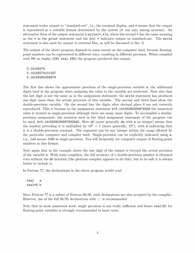
statement writes output to ”standard-out”, i.e., the terminal display, and * means that the outputis reproduced in a suitable format determined by the system (it can vary among systems). Analternative form of the output statement is write(*,*)a, where the second * has the same meaningas the * in the print statement and the first * indicates output to standard-out. The write

statement is also used for output to external files, as will be discussed in Sec. 6.

The output of the above program depends to some extent on the computer used, because floating-point numbers can be represented in different ways, resulting in different precision. When compiledwith f90 on buphy (f90 real.f90) the program produced this output:

3.14159274

3.14159274101257

3.14159265358979

The first line shows the approximate precision of the single-precision variable a; the additionaldigits used in the program when assigning the value to the variable are irrelevant. Note also thatthe last digit is not the same as in the assignment statement; the write statement has producedone digit more than the actual precision of this variable. The second and third lines show thedouble-precision variable. On the second line the digits after decimal place 6 are not correctlyreproduced. This is because in the assignment statement b=3.14159265358979328 the numericalvalue is treated as single-precision although there are many more digits. To accomplish a double-precision assignment, the notation used in the third assignment statement of the program canbe used; b=3.14159265358979328d0. Here d0 (more generally dn with n an integer) means thatthe number preceding it is multiplied by 100 = 1 (more generally, 10n), with d indicating thatit is a double-precision constant. The exponent can be any integer within the range allowed bythe particular computer and compiler used. Single-precision can be explicitly indicated using e,e.g., 1e3 means 1000 in single-precision. You will frequently see computer output of floating-pointnumbers in this format.

Note again that in the example above the last digit of the output is beyond the actual precisionof the variable b. With some compilers, the full accuracy of a double-precision number is obtainedeven without the d0 notation (the gfortran compiler appears to do this), but to be safe it is alwaysbetter to include it.

In Fortran 77, the declarations in the above program would read

real a

real*8 b

Since Fortran 77 is a subset of Fortran 90/95, such declarations are also accepted by the compiler.However, use of the full 90/95 declarations with :: is recommended.

Note that in most numerical work, single precision is not really sufficient and hence real(8) forfloating-point variables is strongly recommended in most cases.

5

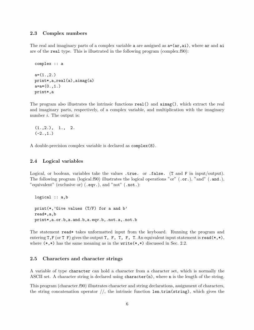
2.3 Complex numbers

The real and imaginary parts of a complex variable a are assigned as a=(ar,ai), where ar and ai

are of the real type. This is illustrated in the following program (complex.f90):

complex :: a

a=(1.,2.)

print*,a,real(a),aimag(a)

a=a*(0.,1.)

print*,a

The program also illustrates the intrinsic functions real() and aimag(), which extract the realand imaginary parts, respectively, of a complex variable, and multiplication with the imaginarynumber i. The output is:

(1.,2.), 1., 2.

(-2.,1.)

A double-precision complex variable is declared as complex(8).

2.4 Logical variables

Logical, or boolean, variables take the values .true. or .false. (T and F in input/output).The following program (logical.f90) illustrates the logical operations ”or” (.or.), ”and” (.and.),”equivalent” (exclusive or) (.eqv.), and ”not” (.not.):

logical :: a,b

print(*,’Give values (T/F) for a and b’

read*,a,b

print*,a.or.b,a.and.b,a.eqv.b,.not.a,.not.b

The statement read* takes unformatted input from the keyboard. Running the program andentering T,F (or T F) gives the output T, F, T, F, T. An equivalent input statement is read(*,*),where (*,*) has the same meaning as in the write(*,*) discussed in Sec. 2.2.

2.5 Characters and character strings

A variable of type character can hold a character from a character set, which is normally theASCII set. A character string is declared using character(n), where n is the length of the string.

This program (character.f90) illustrates character and string declarations, assignment of characters,the string concatenation operator //, the intrinsic function len trim(string), which gives the

6

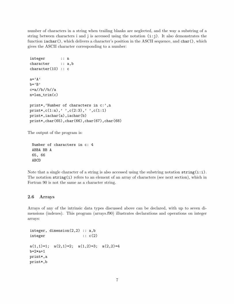
number of characters in a string when trailing blanks are neglected, and the way a substring of astring between characters i and j is accessed using the notation (i:j). It also demonstrates thefunction iachar(), which delivers a character’s position in the ASCII sequence, and char(), whichgives the ASCII character corresponding to a number:

integer :: n

character :: a,b

character(10) :: c

a=’A’

b=’B’

c=a//b//b//a

n=len_trim(c)

print*,’Number of characters in c:’,n

print*,c(1:n),’ ’,c(2:3),’ ’,c(1:1)

print*,iachar(a),iachar(b)

print*,char(65),char(66),char(67),char(68)

The output of the program is:

Number of characters in c: 4

ABBA BB A

65, 66

ABCD

Note that a single character of a string is also accessed using the substring notation string(i:i).The notation string(i) refers to an element of an array of characters (see next section), which inFortran 90 is not the same as a character string.

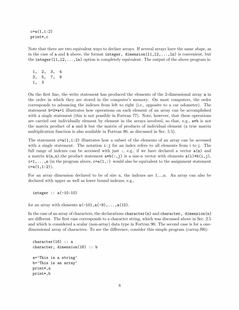
2.6 Arrays

Arrays of any of the intrinsic data types discussed above can be declared, with up to seven di-mensions (indexes). This program (arrays.f90) illustrates declarations and operations on integerarrays:

integer, dimension(2,2) :: a,b

integer :: c(2)

a(1,1)=1; a(2,1)=2; a(1,2)=3; a(2,2)=4

b=2*a+1

print*,a

print*,b

7

c=a(1,1:2)

print*,c

Note that there are two equivalent ways to declare arrays. If several arrays have the same shape, asin the case of a and b above, the format integer, dimension(l1,l2,...,ln) is convenient, butthe integer(l1,l2,...,ln) option is completely equivalent. The output of the above program is:

1, 2, 3, 4

3, 5, 7, 9

1, 3

On the first line, the write statement has produced the elements of the 2-dimensional array a inthe order in which they are stored in the computer’s memory. On most computers, the ordercorresponds to advancing the indexes from left to right (i.e., opposite to a car odometer). Thestatement b=2*a+1 illustrates how operations on each element of an array can be accomplishedwith a single statement (this is not possible in Fortran 77). Note, however, that these operationsare carried out individually element by element in the arrays involved, so that, e.g., a*b is notthe matrix product of a and b but the matrix of products of individual element (a true matrixmultiplication function is also available in Fortran 90, as discussed in Sec. 5.5).

The statement c=a(1,1:2) illustrates how a subset of the elements of an array can be accessedwith a single statement. The notation i:j for an index refers to all elements from i to j. Thefull range of indexes can be accessed with just :, e.g., if we have declared a vector a(n) anda matrix b(n,n),the product statement a*b(:,j) is a size-n vector with elements a(i)*b(i,j),i=1,...,n (in the program above, c=a(1,:) would also be equivalent to the assignment statementc=a(1,1:2)).

For an array dimension declared to be of size n, the indexes are 1,...,n. An array can also bedeclared with upper as well as lower bound indexes, e.g.,

integer :: a(-10:10)

for an array with elements a(-10),a(-9),...,a(10).

In the case of an array of characters, the declarations character(n) and character, dimension(n)

are different. The first case corresponds to a character string, which was discussed above in Sec. 2.5and which is considered a scalar (non-array) data type in Fortran 90. The second case is for a one-dimensional array of characters. To see the difference, consider this simple program (carray.f90):

character(16) :: a

character, dimension(16) :: b

a=’This is a string’

b=’This is an array’

print*,a

print*,b

8

Running it gives this output:

This is a string

TTTTTTTTTTTTTTTT

In the program, a is declared as a string, which is assigned a 16-character sentence. It is repro-duced correctly by the print statement. However, b is an array, and the assignment statementis interpreted as setting each element equal to the first letter of the sentence, because each arrayelement can hold just one character and the = assignment operates on each element of the array.There are several intrinsic procedures for character string manipulations (see Sec. 5.4).

A one dimensional array of m strings is declared by character(n), dimension(m).

2.7 Named constants

A value (of any type) that is not intended to change in the course of the execution of the programcan be declared as a named constant with the parameter statement. An example:

real(8), parameter :: pi=3.14159265358979328d0

The purpose of a named constant, when using it instead of a variable, is that this prohibits anaccidental change of its value. Another useful application is in cases where an array (often severalarrays) has a size which appears in many statements in the program and which the user of theprogram should be able to change easily. This can be achieved by declarations of the type

integer, parameter :: n=10

real(8) :: a(n),b(n,n),c(n,n,n)

Here only the n=10 statement needs to be changed if another array size is required.

2.8 Kind type parameter

In the discussion above we have, for the sake of simplicity in getting started, neglected an importantfeature of type declarations in Fortran 90: In order to ensure that programs are completely portablebetween different computer systems and/or compilers, a kind type parameter should be used insteadof indicating the precision with an integer in a declaration such as real(8) :: a. Here 8 actuallydoes not really refer to the number of bytes used, but to a kind type parameter that on mostcompilers is 4 and 8 for single and double precsision, respectively. However, on some compilers 1is used for single and 2 for double precision—the language standard simply does not (presumablyfor the sake of allowing greater flexibility, although in practice the number of kinds available isvery small and this feature currently seems an unnecessary complication) specify how the kindtype parameter corresponds to the actual precision. To ensure double precision on all systems,the above declaration should be written as real(kind(1d0)) :: a. Here kind() is an intrinsicfunction that gives the kind type parameter of its argument. As an example demonstrating this,

9

one can use this simple program to check the kind type parameter corresponding to single anddouble precison:

print*, kind(1e0)

print*, kind(1d0)

In most cases the output would be 4 and 8.

The reason for using this rather complicated structure is that it, in principle, allows programmersto select any available precision needed. This is done with the function selected real kind(n,m),where n is the desired precision of a floating-point number (number of significant digits) and m isthe range of exponents. For example, the declaration real(selected real kind(10,100) :: a

declares a to have at least 10 significant digits in a range between 10−100 and 10100. However, thereis currently not much point in using this feature since most systems anyway support only standardsingle and double precision. Therefore, a declaration with selected real kind(100,1000)) wouldresult in an error message, since such high precision and large range are not available.

Kind type parameters are available also for the other numerical data types. In this course we willfor sake of simplicity assume that the kind type parameters for real and integer are 4 and 8,which is the case with gfortran (and many other compiler). We will thus not use kind in declarationstatements.

3 Program control constructs

Very important features of a computer program are the abilities to take different actions dependingon various conditions and to repeat code sections multiple times with different data. Here theconstructs for accomplishing branching and loops in the program are discussed.

3.1 Branching with the ”if” statement

The general form of an if...end if construct is

if (logical_a) then

statements_a

else if (logical_b) then

statements_b

else

statements_else

end if

wgere logical i are logical expressions (i.e., taking the values .true. or .false.) and statements i

are code sections to be executed in case the corresponding logical expression is true. Only the state-ments corresponding to the first true expression encountered is executed. There can be an arbitrary

10

number of else if branches. The last else statement is optional; if present the correspondingstatements are executed only if none of the other options is true.

Logical expressions often involve comparisons of variables, e.g., if (a > b) then. In Fortran 90,two forms of the relational operators are used:

equal: == or .eq.

not equal: /= or .ne.

greater than: > or .gt.

less than: < or .lt.

greater than or equal: >= or .ge.

less than or equal: <= or .le.

In Fortran 77, only the two-letter form of the operators to the right is valid.

Here is a very simple example (if.f90) of a program using two nested if...end if constructs:

integer :: int

print*,’Give an integer between 1 and 99’; read*,int

if (int<1.or.int>99) then

print*,’Read the instructions more carefully next time! Good bye.’

else if (int==8.or.int==88) then

print*,’A lucky number; Congratulations!’

else if (int==13) then

print*,’Bad luck...not a good number; beware!’

else

print*,’Nothing special with this number, ’

if (mod(int,2)==0) then

print*,’but I can tell you that it is an even number.’

else

print*,’but I can tell you that it is an odd number.’

end if

end if

The modulus function mod(i,a) gives the remainder of the integer division i/a operation and ishere used with a=2 to determine whether the number int is even or odd.

There is a simpler version of the if construct, of the form

if (logical_expression) statement

where statement is a single statement to be executed if logical expression is true.

11

3.2 The select case construct

In Fortran 90 (but not in Fortran 77), there is another branching construct, the select case, inwhich a single expression of type integer, character or logical is evaluated and different branchescan be taken for specific values, or groups of values, of the expression. This is an example (case.f90)illustrating the select case construct with an integer and a logical expression (the program hasthe same function as the previous one with the if...end if construct):

integer :: int

print*,’Give an integer between 1 and 99’; read*,int

select case (int)

case (:0, 100:)

print*,’Read the instructions more carefully next time! Good bye.’

case (8,88)

print*,’A lucky number; Congratulations!’

case (13)

print*,’Bad luck...not a good number; beware!’

case default

print*,’Nothing special with this number,’

select case (mod(int,2)==0)

case (.true.)

print*,’but I can tell you that it is an even number.’

case (.false.)

print*,’but I can tell you that it is an odd number.’

end select

end select

Any number of specific values can be listed within () in the case() statement, or a range (orseveral ranges) of values can be specified using i:j for all values between i and j, :i for all valuesless than or equal to i, or i: for all values greater than or equal to i. Note that the differentcase-groups must be non-overlapping.

3.3 Loops

In Fortran, repeated execution of a code section is accomplished with do loops. This is an example(doloop1.f90) in which the squares of the numbers 1,...,n are produced:

integer :: i,n

print*,’Give highest number n to be squared’; read*,n

do i=1,n

print*,i**2

end do

12

To increment by more than 1 in each execution of the loop, the form do i=1,n,m is used, where m

is the increment. If n is not divisible by m, the last step of the loop is the highest i for which m*i

< n.

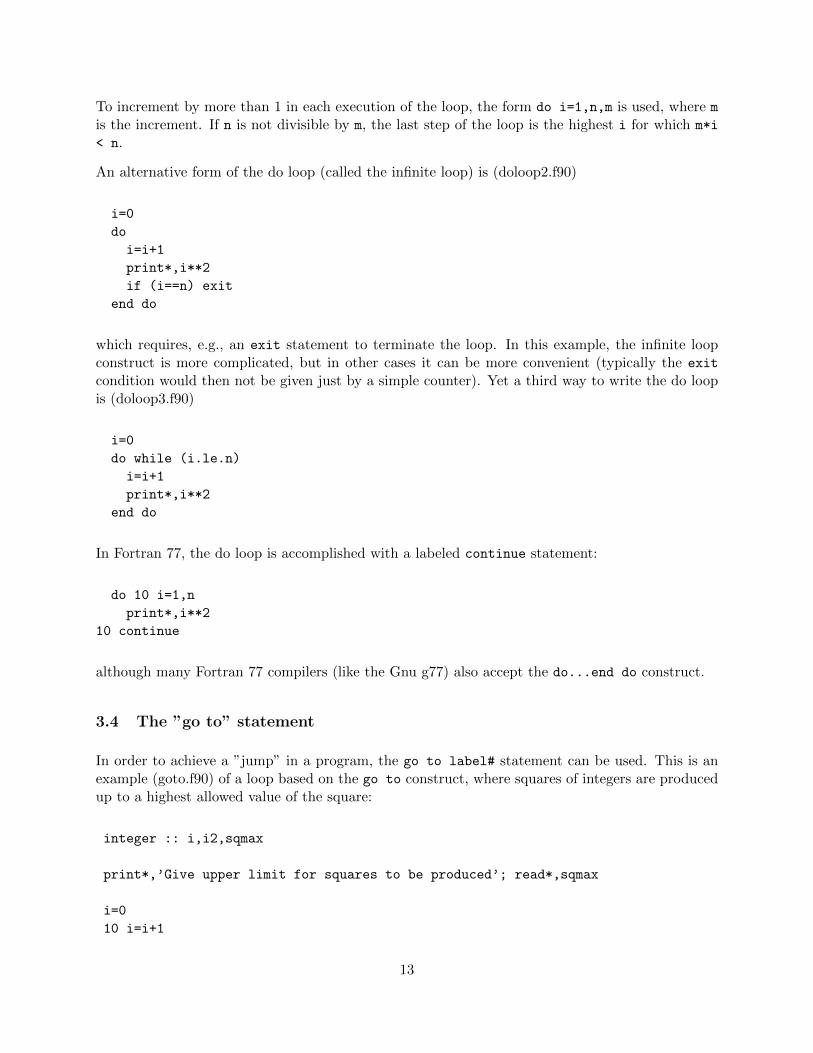
An alternative form of the do loop (called the infinite loop) is (doloop2.f90)

i=0

do

i=i+1

print*,i**2

if (i==n) exit

end do

which requires, e.g., an exit statement to terminate the loop. In this example, the infinite loopconstruct is more complicated, but in other cases it can be more convenient (typically the exit

condition would then not be given just by a simple counter). Yet a third way to write the do loopis (doloop3.f90)

i=0

do while (i.le.n)

i=i+1

print*,i**2

end do

In Fortran 77, the do loop is accomplished with a labeled continue statement:

do 10 i=1,n

print*,i**2

10 continue

although many Fortran 77 compilers (like the Gnu g77) also accept the do...end do construct.

3.4 The ”go to” statement

In order to achieve a ”jump” in a program, the go to label# statement can be used. This is anexample (goto.f90) of a loop based on the go to construct, where squares of integers are producedup to a highest allowed value of the square:

integer :: i,i2,sqmax

print*,’Give upper limit for squares to be produced’; read*,sqmax

i=0

10 i=i+1

13

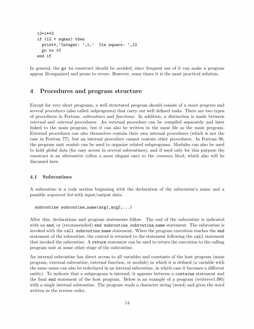
i2=i**2

if (i2 < sqmax) then

print*,’Integer: ’,i,’ Its square: ’,i2

go to 10

end if

In general, the go to construct should be avoided, since frequent use of it can make a programappear ill-organized and prone to errors. However, some times it is the most practical solution.

4 Procedures and program structure

Except for very short programs, a well structured program should consist of a main program andseveral procedures (also called subprograms) that carry out well defined tasks. There are two typesof procedures in Fortran; subroutines and functions. In addition, a distinction is made betweeninternal and external procedures. An external procedure can be compiled separately and laterlinked to the main program, but it can also be written in the same file as the main program.External procedures can also themselves contain their own internal procedures (which is not thecase in Fortran 77), but an internal procedure cannot contain other procedures. In Fortran 90,the program unit module can be used to organize related subprograms. Modules can also be usedto hold global data (for easy access in several subroutines), and if used only for this purpose theconstruct is an alternative (often a more elegant one) to the common block, which also will bediscussed here.

4.1 Subroutines

A subroutine is a code section beginning with the declaration of the subroutine’s name and apossible argument list with input/output data:

subroutine subroutine_name(arg1,arg2,...)

After this, declarations and program statements follow. The end of the subroutine is indicatedwith an end, or (recommended) end subroutine subroutine name statement. The subroutine isinvoked with the call subroutine name statement. When the program execution reaches the end

statement of the subroutine, the control is returned to the statement following the call statementthat invoked the subroutine. A return statement can be used to return the execution to the callingprogram unit at some other stage of the subroutine.

An internal subroutine has direct access to all variables and constants of the host program (mainprogram, external subroutine, external function, or module) in which it is defined (a variable withthe same name can also be redeclared in an internal subroutine, in which case it becomes a differententity). To indicate that a subprogram is internal, it appears between a contains statement andthe final end statement of the host program. Below is an example of a program (writerev1.f90)with a single internal subroutine. The program reads a character string (word) and gives the wordwritten in the reverse order.

14

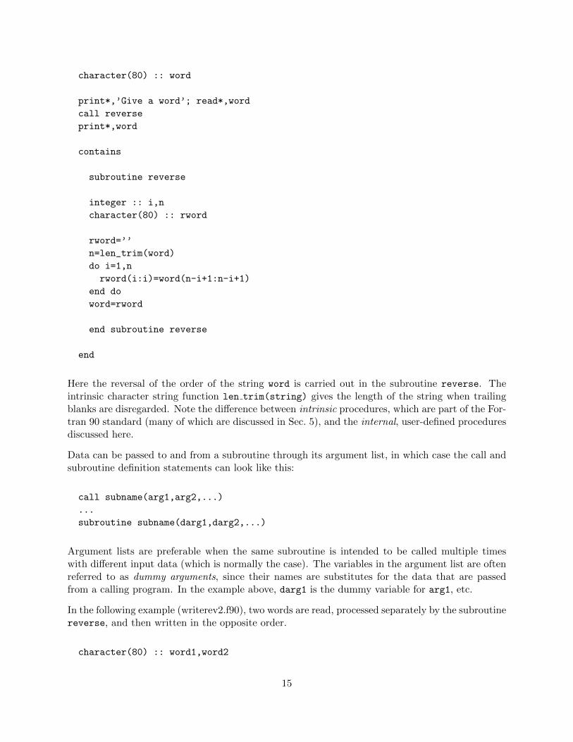
character(80) :: word

print*,’Give a word’; read*,word

call reverse

print*,word

contains

subroutine reverse

integer :: i,n

character(80) :: rword

rword=’’

n=len_trim(word)

do i=1,n

rword(i:i)=word(n-i+1:n-i+1)

end do

word=rword

end subroutine reverse

end

Here the reversal of the order of the string word is carried out in the subroutine reverse. Theintrinsic character string function len trim(string) gives the length of the string when trailingblanks are disregarded. Note the difference between intrinsic procedures, which are part of the For-tran 90 standard (many of which are discussed in Sec. 5), and the internal, user-defined proceduresdiscussed here.

Data can be passed to and from a subroutine through its argument list, in which case the call andsubroutine definition statements can look like this:

call subname(arg1,arg2,...)

...

subroutine subname(darg1,darg2,...)

Argument lists are preferable when the same subroutine is intended to be called multiple timeswith different input data (which is normally the case). The variables in the argument list are oftenreferred to as dummy arguments, since their names are substitutes for the data that are passedfrom a calling program. In the example above, darg1 is the dummy variable for arg1, etc.

In the following example (writerev2.f90), two words are read, processed separately by the subroutinereverse, and then written in the opposite order.

character(80) :: word1,word2

15

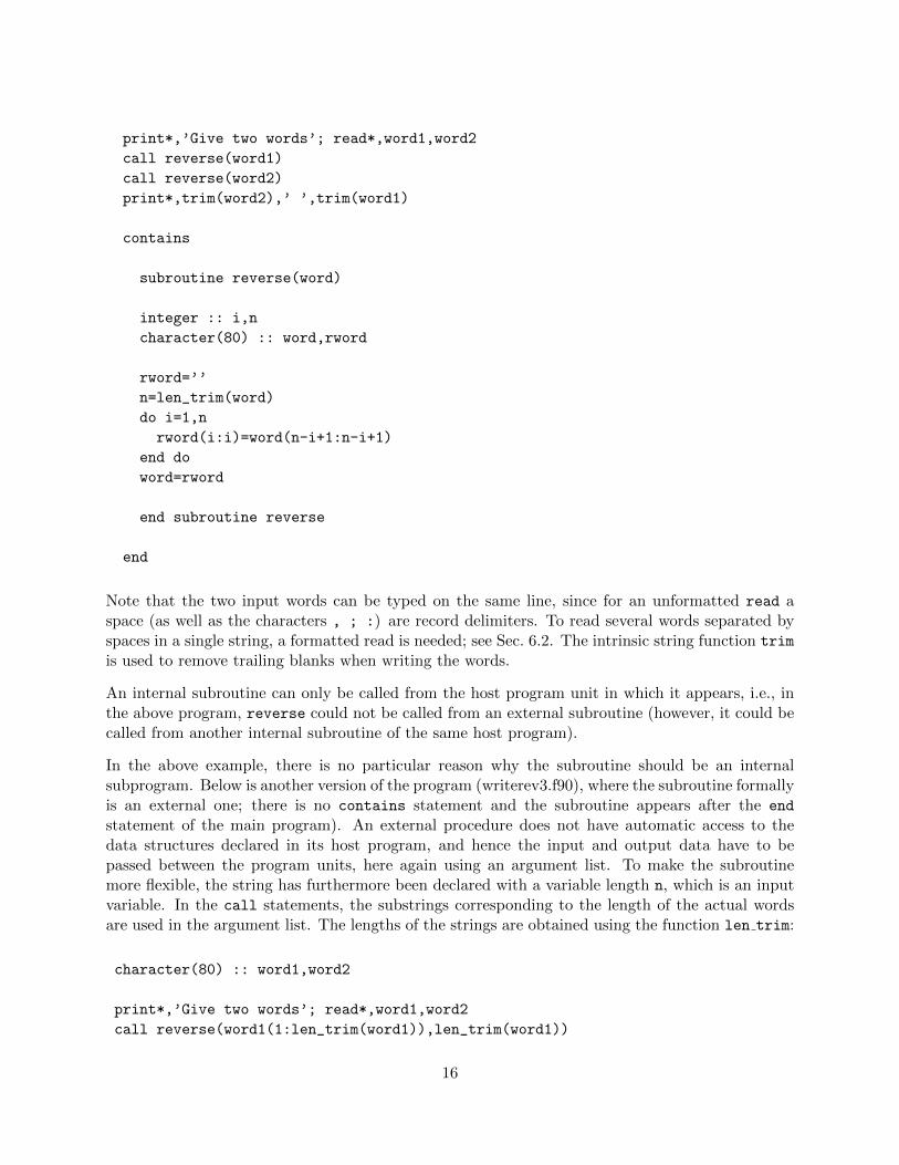
print*,’Give two words’; read*,word1,word2

call reverse(word1)

call reverse(word2)

print*,trim(word2),’ ’,trim(word1)

contains

subroutine reverse(word)

integer :: i,n

character(80) :: word,rword

rword=’’

n=len_trim(word)

do i=1,n

rword(i:i)=word(n-i+1:n-i+1)

end do

word=rword

end subroutine reverse

end

Note that the two input words can be typed on the same line, since for an unformatted read aspace (as well as the characters , ; :) are record delimiters. To read several words separated byspaces in a single string, a formatted read is needed; see Sec. 6.2. The intrinsic string function trim

is used to remove trailing blanks when writing the words.

An internal subroutine can only be called from the host program unit in which it appears, i.e., inthe above program, reverse could not be called from an external subroutine (however, it could becalled from another internal subroutine of the same host program).

In the above example, there is no particular reason why the subroutine should be an internalsubprogram. Below is another version of the program (writerev3.f90), where the subroutine formallyis an external one; there is no contains statement and the subroutine appears after the end

statement of the main program). An external procedure does not have automatic access to thedata structures declared in its host program, and hence the input and output data have to bepassed between the program units, here again using an argument list. To make the subroutinemore flexible, the string has furthermore been declared with a variable length n, which is an inputvariable. In the call statements, the substrings corresponding to the length of the actual wordsare used in the argument list. The lengths of the strings are obtained using the function len trim:

character(80) :: word1,word2

print*,’Give two words’; read*,word1,word2

call reverse(word1(1:len_trim(word1)),len_trim(word1))

16

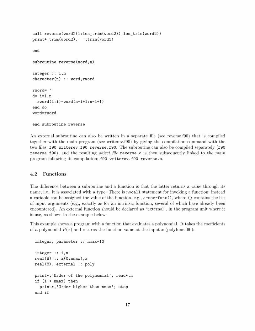
call reverse(word2(1:len_trim(word2)),len_trim(word2))

print*,trim(word2),’ ’,trim(word1)

end

subroutine reverse(word,n)

integer :: i,n

character(n) :: word,rword

rword=’’

do i=1,n

rword(i:i)=word(n-i+1:n-i+1)

end do

word=rword

end subroutine reverse

An external subroutine can also be written in a separate file (see reverse.f90) that is compiledtogether with the main program (see writerev.f90) by giving the compilation command with thetwo files; f90 writerev.f90 reverse.f90. The subroutine can also be compiled separately (f90reverse.f90), and the resulting object file reverse.o is then subsequently linked to the mainprogram following its compilation; f90 writerev.f90 reverse.o.

4.2 Functions

The difference between a subroutine and a function is that the latter returns a value through itsname, i.e., it is associated with a type. There is nocall statement for invoking a function; insteada variable can be assigned the value of the function, e.g., a=userfunc(), where () contains the listof input arguments (e.g., exactly as for an intrinsic function, several of which have already beenencountered). An external function should be declared as “external”, in the program unit where itis use, as shown in the example below.

This example shows a program with a function that evaluates a polynomial. It takes the coefficientsof a polynomial P (x) and returns the function value at the input x (polyfunc.f90):

integer, parameter :: nmax=10

integer :: i,n

real(8) :: a(0:nmax),x

real(8), external :: poly

print*,’Order of the polynomial’; read*,n

if (i > nmax) then

print*,’Order higher than nmax’; stop

end if

17

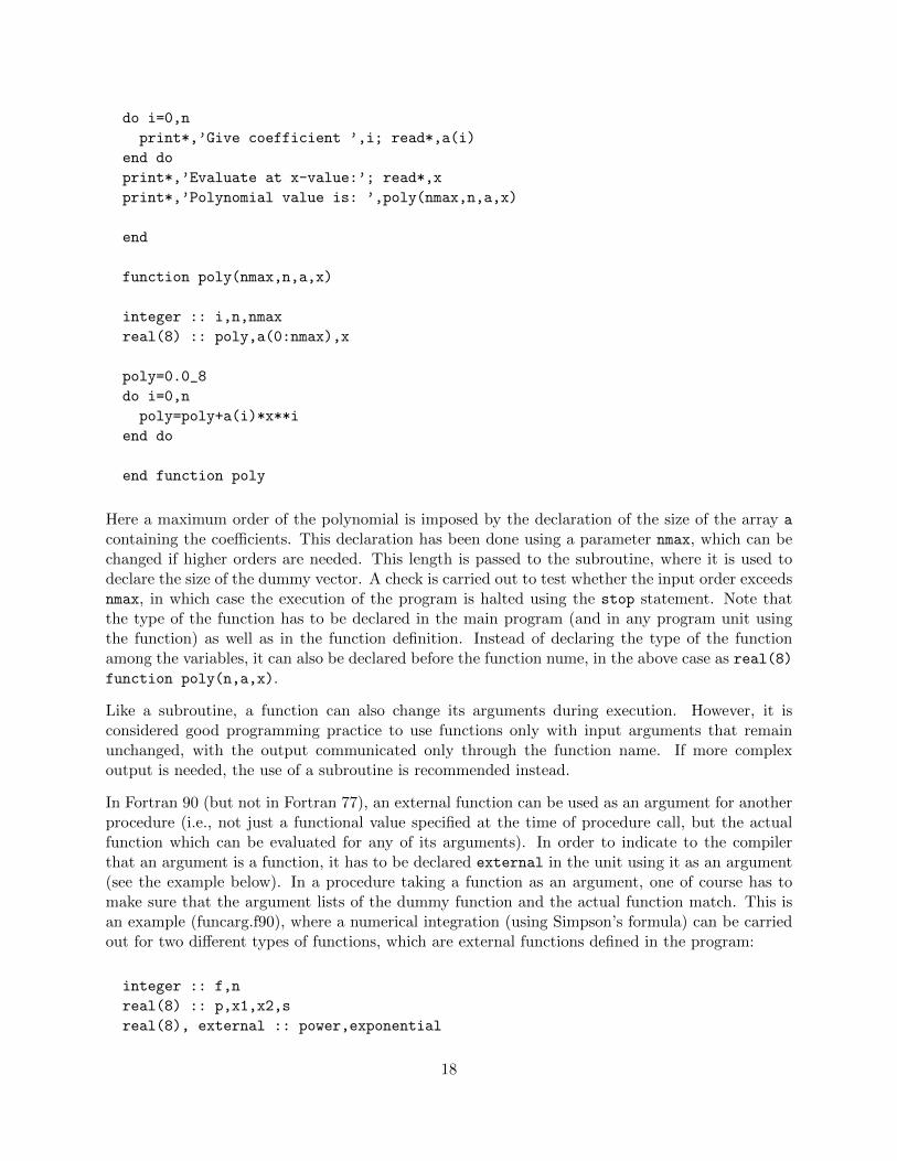
do i=0,n

print*,’Give coefficient ’,i; read*,a(i)

end do

print*,’Evaluate at x-value:’; read*,x

print*,’Polynomial value is: ’,poly(nmax,n,a,x)

end

function poly(nmax,n,a,x)

integer :: i,n,nmax

real(8) :: poly,a(0:nmax),x

poly=0.0_8

do i=0,n

poly=poly+a(i)*x**i

end do

end function poly

Here a maximum order of the polynomial is imposed by the declaration of the size of the array a

containing the coefficients. This declaration has been done using a parameter nmax, which can bechanged if higher orders are needed. This length is passed to the subroutine, where it is used todeclare the size of the dummy vector. A check is carried out to test whether the input order exceedsnmax, in which case the execution of the program is halted using the stop statement. Note thatthe type of the function has to be declared in the main program (and in any program unit usingthe function) as well as in the function definition. Instead of declaring the type of the functionamong the variables, it can also be declared before the function nume, in the above case as real(8)function poly(n,a,x).

Like a subroutine, a function can also change its arguments during execution. However, it isconsidered good programming practice to use functions only with input arguments that remainunchanged, with the output communicated only through the function name. If more complexoutput is needed, the use of a subroutine is recommended instead.

In Fortran 90 (but not in Fortran 77), an external function can be used as an argument for anotherprocedure (i.e., not just a functional value specified at the time of procedure call, but the actualfunction which can be evaluated for any of its arguments). In order to indicate to the compilerthat an argument is a function, it has to be declared external in the unit using it as an argument(see the example below). In a procedure taking a function as an argument, one of course has tomake sure that the argument lists of the dummy function and the actual function match. This isan example (funcarg.f90), where a numerical integration (using Simpson’s formula) can be carriedout for two different types of functions, which are external functions defined in the program:

integer :: f,n

real(8) :: p,x1,x2,s

real(8), external :: power,exponential

18

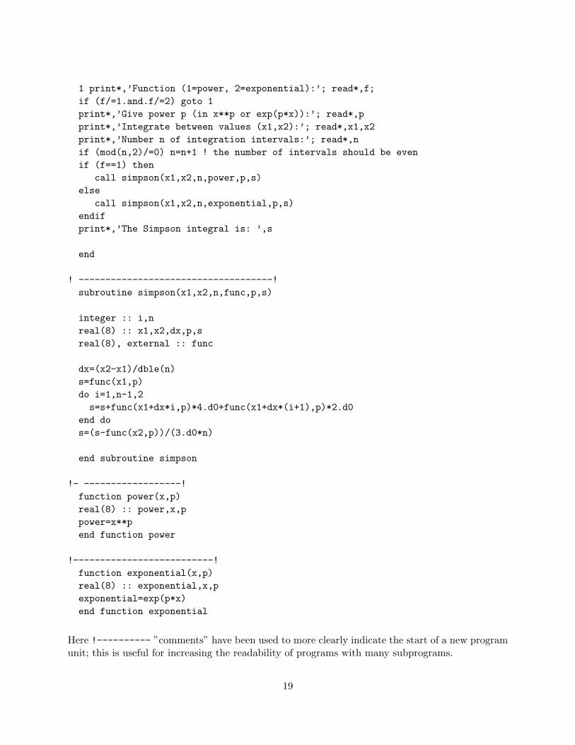
1 print*,’Function (1=power, 2=exponential):’; read*,f;

if (f/=1.and.f/=2) goto 1

print*,’Give power p (in x**p or exp(p*x)):’; read*,p

print*,’Integrate between values (x1,x2):’; read*,x1,x2

print*,’Number n of integration intervals:’; read*,n

if (mod(n,2)/=0) n=n+1 ! the number of intervals should be even

if (f==1) then

call simpson(x1,x2,n,power,p,s)

else

call simpson(x1,x2,n,exponential,p,s)

endif

print*,’The Simpson integral is: ’,s

end

! ------------------------------------!

subroutine simpson(x1,x2,n,func,p,s)

integer :: i,n

real(8) :: x1,x2,dx,p,s

real(8), external :: func

dx=(x2-x1)/dble(n)

s=func(x1,p)

do i=1,n-1,2

s=s+func(x1+dx*i,p)*4.d0+func(x1+dx*(i+1),p)*2.d0

end do

s=(s-func(x2,p))/(3.d0*n)

end subroutine simpson

!- ------------------!

function power(x,p)

real(8) :: power,x,p

power=x**p

end function power

!--------------------------!

function exponential(x,p)

real(8) :: exponential,x,p

exponential=exp(p*x)

end function exponential

Here !---------- ”comments” have been used to more clearly indicate the start of a new programunit; this is useful for increasing the readability of programs with many subprograms.

19

4.3 Common blocks

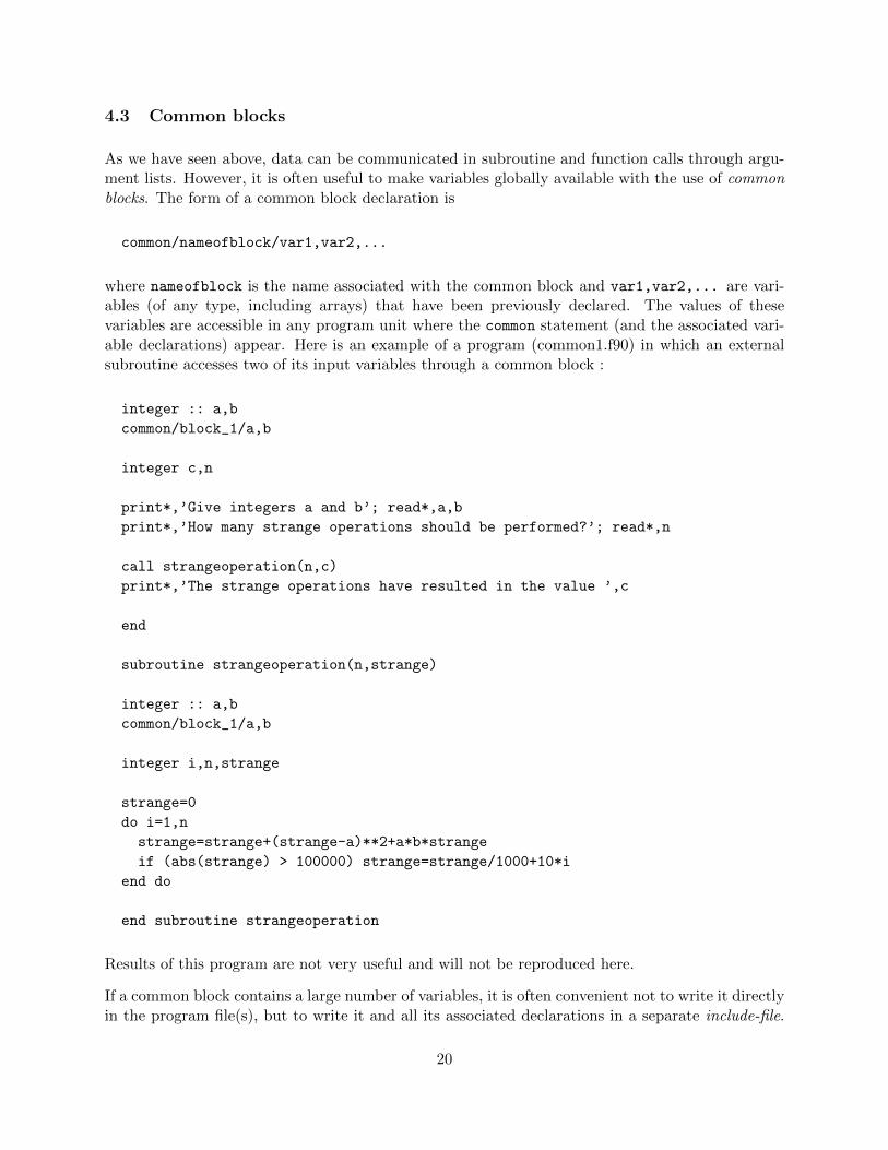
As we have seen above, data can be communicated in subroutine and function calls through argu-ment lists. However, it is often useful to make variables globally available with the use of commonblocks. The form of a common block declaration is

common/nameofblock/var1,var2,...

where nameofblock is the name associated with the common block and var1,var2,... are vari-ables (of any type, including arrays) that have been previously declared. The values of thesevariables are accessible in any program unit where the common statement (and the associated vari-able declarations) appear. Here is an example of a program (common1.f90) in which an externalsubroutine accesses two of its input variables through a common block :

integer :: a,b

common/block_1/a,b

integer c,n

print*,’Give integers a and b’; read*,a,b

print*,’How many strange operations should be performed?’; read*,n

call strangeoperation(n,c)

print*,’The strange operations have resulted in the value ’,c

end

subroutine strangeoperation(n,strange)

integer :: a,b

common/block_1/a,b

integer i,n,strange

strange=0

do i=1,n

strange=strange+(strange-a)**2+a*b*strange

if (abs(strange) > 100000) strange=strange/1000+10*i

end do

end subroutine strangeoperation

Results of this program are not very useful and will not be reproduced here.

If a common block contains a large number of variables, it is often convenient not to write it directlyin the program file(s), but to write it and all its associated declarations in a separate include-file.

20

With such a file, common.h, containing the above common block and its declarations (as in C/C++programs, the ending .h is often used for include-files);

integer :: a,b

common/block_1/a,b

the statement include ’common.h’ should replace these lines in the program (in both the mainprogram and the subroutine). The contents of the file are then inserted at the compilation stage.The use of an include-file is illustrated in the program common2.f90, which uses the supplied includefile common.h (see the web page).

Common blocks are frequently used in Fortran 77. However, in Fortran 90 the use of modules is inmost cases recommended instead, as discussed next.

4.4 Modules

In the simplest case, a module contains named constants and variables, for the purpose of easyaccess to such data in several subprograms (i.e., global data, similar to common blocks). Such amodule can look like this:

module powermodule

integer, parameter :: nd=10, np=3

real(8) :: xpowers(np,nd)

end module powermodule

The constants and the array are accessible in any subprogram (or the main program) that includesthe statement use powermodule, which should appear before all declaration statements in theprogram unit (also before a possible implicit none statement).

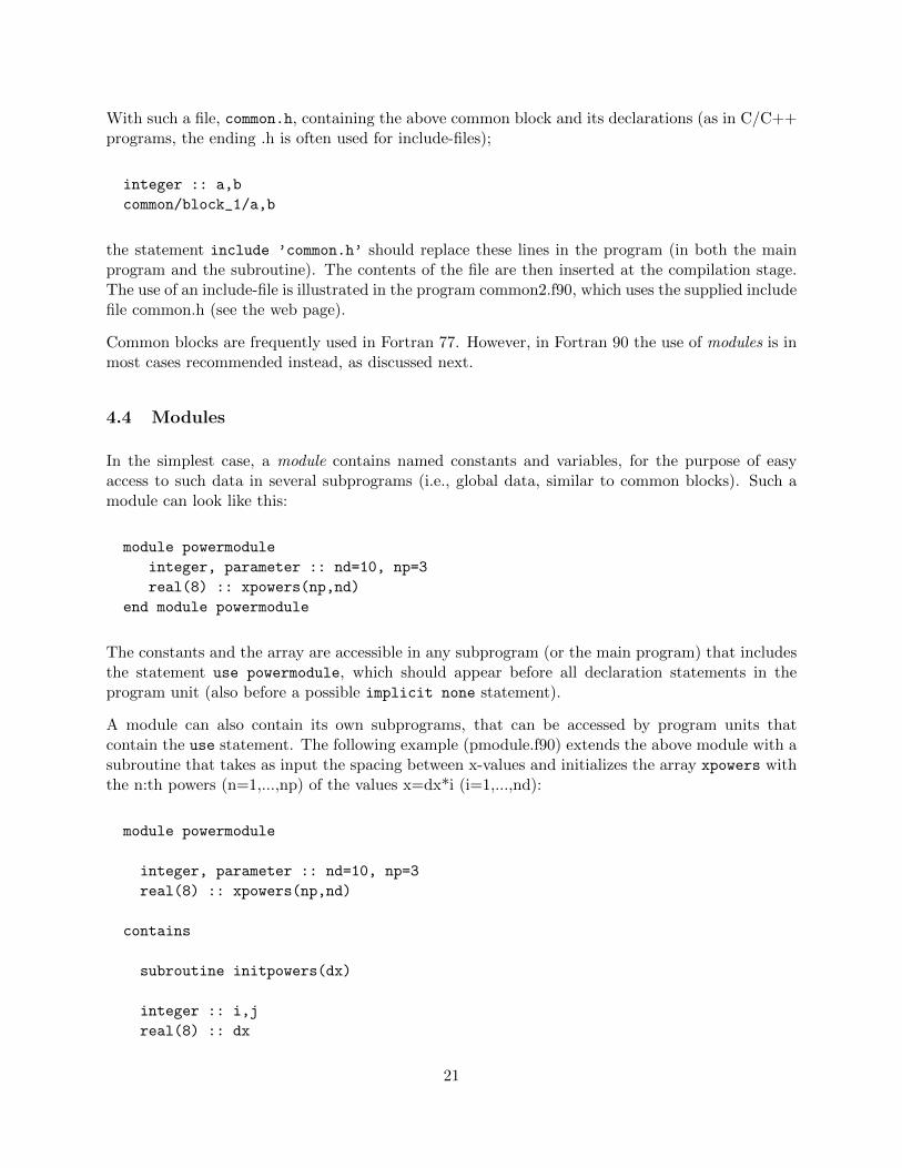
A module can also contain its own subprograms, that can be accessed by program units thatcontain the use statement. The following example (pmodule.f90) extends the above module with asubroutine that takes as input the spacing between x-values and initializes the array xpowers withthe n:th powers (n=1,...,np) of the values x=dx*i (i=1,...,nd):

module powermodule

integer, parameter :: nd=10, np=3

real(8) :: xpowers(np,nd)

contains

subroutine initpowers(dx)

integer :: i,j

real(8) :: dx

21

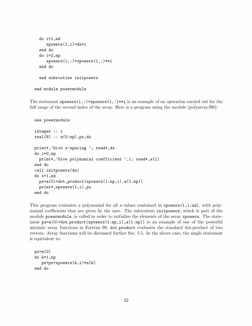
do i=1,nd

xpowers(1,i)=dx*i

end do

do i=2,np

xpowers(i,:)=xpowers(1,:)**i

end do

end subroutine initpowers

end module powermodule

The statement xpowers(i,:)=xpowers(1,:)**i is an example of an operation carried out for thefull range of the second index of the array. Here is a program using the module (polyarray.f90):

use powermodule

integer :: i

real(8) :: a(0:np),px,dx

print*,’Give x-spacing ’; read*,dx

do i=0,np

print*,’Give polynomial coefficient ’,i; read*,a(i)

end do

call initpowers(dx)

do i=1,nd

px=a(0)+dot_product(xpowers(1:np,i),a(1:np))

print*,xpowers(1,i),px

end do

This program evaluates a polynomial for all x-values contained in xpowers(1,1:nd), with poly-nomial coefficients that are given by the user. The subroutine initpowers, which is part of themodule powermodule, is called in order to initialize the elements of the array xpowers. The state-ment px=a(0)+dot product(xpowers(1:np,i),a(1:np)) is an example of one of the powerfulintrinsic array functions in Fortran 90; dot product evaluates the standard dot-product of twovectors. Array functions will be discussed further Sec. 5.5. In the above case, the single statementis equivalent to:

px=a(0)

do k=1,np

px=px+xpowers(k,i)*a(k)

end do

22

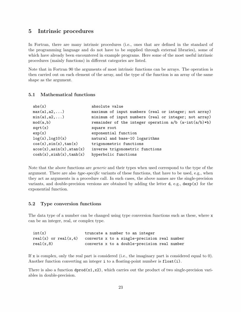
5 Intrinsic procedures

In Fortran, there are many intrinsic procedures (i.e., ones that are defined in the standard ofthe programming language and do not have to be supplied through external libraries), some ofwhich have already been encountered in example programs. Here some of the most useful intrinsicprocedures (mainly functions) in different categories are listed.

Note that in Fortran 90 the arguments of most intrinsic functions can be arrays. The operation isthen carried out on each element of the array, and the type of the function is an array of the sameshape as the argument.

5.1 Mathematical functions

abs(x) absolute value

max(a1,a2,...) maximum of input numbers (real or integer; not array)

min(a1,a2,...) minimum of input numbers (real or integer; not array)

mod(a,b) remainder of the integer operation a/b (a-int(a/b)*b)

sqrt(x) square root

exp(x) exponential function

log(x),log10(x) natural and base-10 logarithms

cos(x),sin(x),tan(x) trigonometric functions

acos(x),asin(x),atan(x) inverse trigonometric functions

cosh(x),sinh(x),tanh(x) hyperbolic functions

Note that the above functions are generic and their types when used correspond to the type of theargument. There are also type-specific variants of these functions, that have to be used, e.g., whenthey act as arguments in a procedure call. In such cases, the above names are the single-precisionvariants, and double-precision versions are obtained by adding the letter d, e.g., dexp(x) for theexponential function.

5.2 Type conversion functions

The data type of a number can be changed using type conversion functions such as these, where x

can be an integer, real, or complex type.

int(x) truncate a number to an integer

real(x) or real(x,4) converts x to a single-precision real number

real(x,8) converts x to a double-precision real number

If x is complex, only the real part is considered (i.e., the imaginary part is considered equal to 0).Another function converting an integer i to a floating-point number is float(i).

There is also a function dprod(x1,x2), which carries out the product of two single-precision vari-ables in double-precision.

23

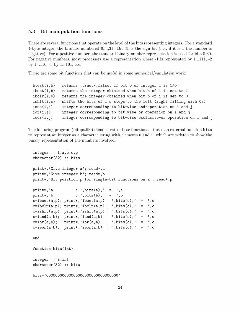
5.3 Bit manipulation functions

There are several functions that operate on the level of the bits representing integers. For a standard4-byte integer, the bits are numbered 0,...,31. Bit 31 is the sign bit (i.e., if it is 1 the number isnegative). For a positive number, the standard binary-number representation is used for bits 0-30.For negative numbers, most processors use a representation where -1 is represented by 1...111, -2by 1...110, -3 by 1...101, etc.

These are some bit functions that can be useful in some numerical/simulation work:

btest(i,b) returns .true./.false. if bit b of integer i is 1/0

ibset(i,b) returns the integer obtained when bit b of i is set to 1

ibclr(i,b) returns the integer obtained when bit b of i is set to 0

ishft(i,s) shifts the bits of i s steps to the left (right filling with 0s)

iand(i,j) integer corresponding to bit-wise and-operation on i and j

ior(i,j) integer corresponding to bit-wise or-operation on i and j

ieor(i,j) integer corresponding to bit-wise exclusive-or operation on i and j

The following program (bitops.f90) demonstrates these functions. It uses an external function bits

to represent an integer as a character string with elements 0 and 1, which are written to show thebinary representation of the numbers involved.

integer :: i,a,b,c,p

character(32) :: bits

print*,’Give integer a’; read*,a

print*,’Give integer b’; read*,b

print*,’Bit position p for single-bit functions on a’; read*,p

print*,’a : ’,bits(a),’ = ’,a

print*,’b : ’,bits(b),’ = ’,b

c=ibset(a,p); print*,’ibset(a,p) : ’,bits(c),’ = ’,c

c=ibclr(a,p); print*,’ibclr(a,p) : ’,bits(c),’ = ’,c

c=ishft(a,p); print*,’ishft(a,p) : ’,bits(c),’ = ’,c

c=iand(a,b); print*,’iand(a,b) : ’,bits(c),’ = ’,c

c=ior(a,b); print*,’ior(a,b) : ’,bits(c),’ = ’,c

c=ieor(a,b); print*,’ieor(a,b) : ’,bits(c),’ = ’,c

end

function bits(int)

integer :: i,int

character(32) :: bits

bits=’00000000000000000000000000000000’

24

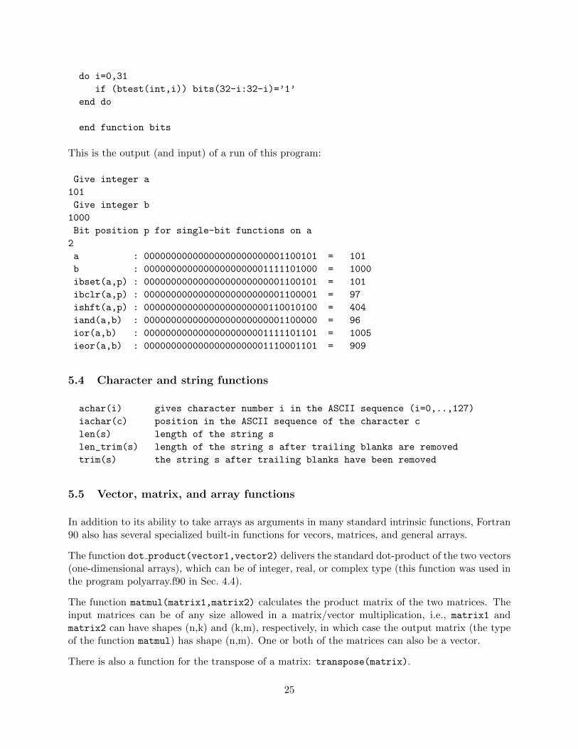
do i=0,31

if (btest(int,i)) bits(32-i:32-i)=’1’

end do

end function bits

This is the output (and input) of a run of this program:

Give integer a

101

Give integer b

1000

Bit position p for single-bit functions on a

2

a : 00000000000000000000000001100101 = 101

b : 00000000000000000000001111101000 = 1000

ibset(a,p) : 00000000000000000000000001100101 = 101

ibclr(a,p) : 00000000000000000000000001100001 = 97

ishft(a,p) : 00000000000000000000000110010100 = 404

iand(a,b) : 00000000000000000000000001100000 = 96

ior(a,b) : 00000000000000000000001111101101 = 1005

ieor(a,b) : 00000000000000000000001110001101 = 909

5.4 Character and string functions

achar(i) gives character number i in the ASCII sequence (i=0,..,127)

iachar(c) position in the ASCII sequence of the character c

len(s) length of the string s

len_trim(s) length of the string s after trailing blanks are removed

trim(s) the string s after trailing blanks have been removed

5.5 Vector, matrix, and array functions

In addition to its ability to take arrays as arguments in many standard intrinsic functions, Fortran90 also has several specialized built-in functions for vecors, matrices, and general arrays.

The function dot product(vector1,vector2) delivers the standard dot-product of the two vectors(one-dimensional arrays), which can be of integer, real, or complex type (this function was used inthe program polyarray.f90 in Sec. 4.4).

The function matmul(matrix1,matrix2) calculates the product matrix of the two matrices. Theinput matrices can be of any size allowed in a matrix/vector multiplication, i.e., matrix1 andmatrix2 can have shapes (n,k) and (k,m), respectively, in which case the output matrix (the typeof the function matmul) has shape (n,m). One or both of the matrices can also be a vector.

There is also a function for the transpose of a matrix: transpose(matrix).

25

These are some other useful functions for an array with any number of dimensions:

sum(array) sum of the elements of the array

product(array) product of the elements of the array

minval(array) minimum of the elements of an integer or real array

maxval(array) maximum of the elements of an integer or real array

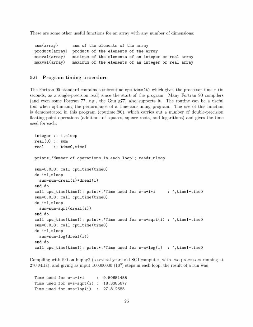
5.6 Program timing procedure

The Fortran 95 standard contains a subroutine cpu time(t) which gives the processor time t (inseconds, as a single-precision real) since the start of the program. Many Fortran 90 compilers(and even some Fortran 77, e.g., the Gnu g77) also supports it. The routine can be a usefultool when optimizing the performance of a time-consuming program. The use of this functionis demonstrated in this program (cputime.f90), which carries out a number of double-precisionfloating-point operations (additions of squares, square roots, and logarithms) and gives the timeused for each.

integer :: i,nloop

real(8) :: sum

real :: time0,time1

print*,’Number of operations in each loop’; read*,nloop

sum=0.0_8; call cpu_time(time0)

do i=1,nloop

sum=sum+dreal(i)*dreal(i)

end do

call cpu_time(time1); print*,’Time used for s=s+i*i : ’,time1-time0

sum=0.0_8; call cpu_time(time0)

do i=1,nloop

sum=sum+sqrt(dreal(i))

end do

call cpu_time(time1); print*,’Time used for s=s+sqrt(i) : ’,time1-time0

sum=0.0_8; call cpu_time(time0)

do i=1,nloop

sum=sum+log(dreal(i))

end do

call cpu_time(time1); print*,’Time used for s=s+log(i) : ’,time1-time0

Compiling with f90 on buphy2 (a several years old SGI computer, with two processors running at270 MHz), and giving as input 100000000 (108) steps in each loop, the result of a run was

Time used for s=s+i*i : 9.50651455

Time used for s=s+sqrt(i) : 18.3385677

Time used for s=s+log(i) : 27.812685

26

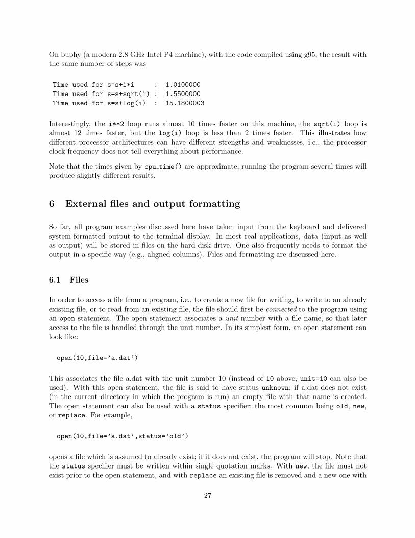
On buphy (a modern 2.8 GHz Intel P4 machine), with the code compiled using g95, the result withthe same number of steps was

Time used for s=s+i*i : 1.0100000

Time used for s=s+sqrt(i) : 1.5500000

Time used for s=s+log(i) : 15.1800003

Interestingly, the i**2 loop runs almost 10 times faster on this machine, the sqrt(i) loop isalmost 12 times faster, but the log(i) loop is less than 2 times faster. This illustrates howdifferent processor architectures can have different strengths and weaknesses, i.e., the processorclock-frequency does not tell everything about performance.

Note that the times given by cpu time() are approximate; running the program several times willproduce slightly different results.

6 External files and output formatting

So far, all program examples discussed here have taken input from the keyboard and deliveredsystem-formatted output to the terminal display. In most real applications, data (input as wellas output) will be stored in files on the hard-disk drive. One also frequently needs to format theoutput in a specific way (e.g., aligned columns). Files and formatting are discussed here.

6.1 Files

In order to access a file from a program, i.e., to create a new file for writing, to write to an alreadyexisting file, or to read from an existing file, the file should first be connected to the program usingan open statement. The open statement associates a unit number with a file name, so that lateraccess to the file is handled through the unit number. In its simplest form, an open statement canlook like:

open(10,file=’a.dat’)

This associates the file a.dat with the unit number 10 (instead of 10 above, unit=10 can also beused). With this open statement, the file is said to have status unknown; if a.dat does not exist(in the current directory in which the program is run) an empty file with that name is created.The open statement can also be used with a status specifier; the most common being old, new,or replace. For example,

open(10,file=’a.dat’,status=’old’)

opens a file which is assumed to already exist; if it does not exist, the program will stop. Note thatthe status specifier must be written within single quotation marks. With new, the file must notexist prior to the open statement, and with replace an existing file is removed and a new one with

27

the same name is created. Without an explicit status specifier, the default is unknown, which onmost systems is the same as replace.

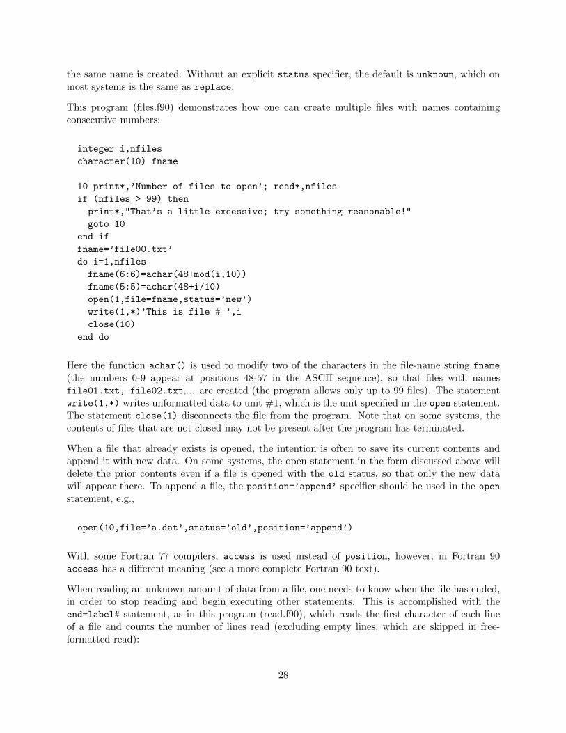
This program (files.f90) demonstrates how one can create multiple files with names containingconsecutive numbers:

integer i,nfiles

character(10) fname

10 print*,’Number of files to open’; read*,nfiles

if (nfiles > 99) then

print*,"That’s a little excessive; try something reasonable!"

goto 10

end if

fname=’file00.txt’

do i=1,nfiles

fname(6:6)=achar(48+mod(i,10))

fname(5:5)=achar(48+i/10)

open(1,file=fname,status=’new’)

write(1,*)’This is file # ’,i

close(10)

end do

Here the function achar() is used to modify two of the characters in the file-name string fname

(the numbers 0-9 appear at positions 48-57 in the ASCII sequence), so that files with namesfile01.txt, file02.txt,... are created (the program allows only up to 99 files). The statementwrite(1,*) writes unformatted data to unit #1, which is the unit specified in the open statement.The statement close(1) disconnects the file from the program. Note that on some systems, thecontents of files that are not closed may not be present after the program has terminated.

When a file that already exists is opened, the intention is often to save its current contents andappend it with new data. On some systems, the open statement in the form discussed above willdelete the prior contents even if a file is opened with the old status, so that only the new datawill appear there. To append a file, the position=’append’ specifier should be used in the open

statement, e.g.,

open(10,file=’a.dat’,status=’old’,position=’append’)

With some Fortran 77 compilers, access is used instead of position, however, in Fortran 90access has a different meaning (see a more complete Fortran 90 text).

When reading an unknown amount of data from a file, one needs to know when the file has ended,in order to stop reading and begin executing other statements. This is accomplished with theend=label# statement, as in this program (read.f90), which reads the first character of each lineof a file and counts the number of lines read (excluding empty lines, which are skipped in free-formatted read):

28

integer :: nlines

character :: c

character(16) :: fname

print*,’Give a file:’;read*,fname

open(1,file=fname,status=’old’)

nlines=0

do

read(1,*,end=10)c; print*,c

nlines=nlines+1

end do

10 close(1)

print*; print*,’The number of non-empty lines in the file is:’,nlines

Try it with one of the program files as input!

6.2 Format statements

So far, examples have been given of terminal and file output with a default format, indicated by *

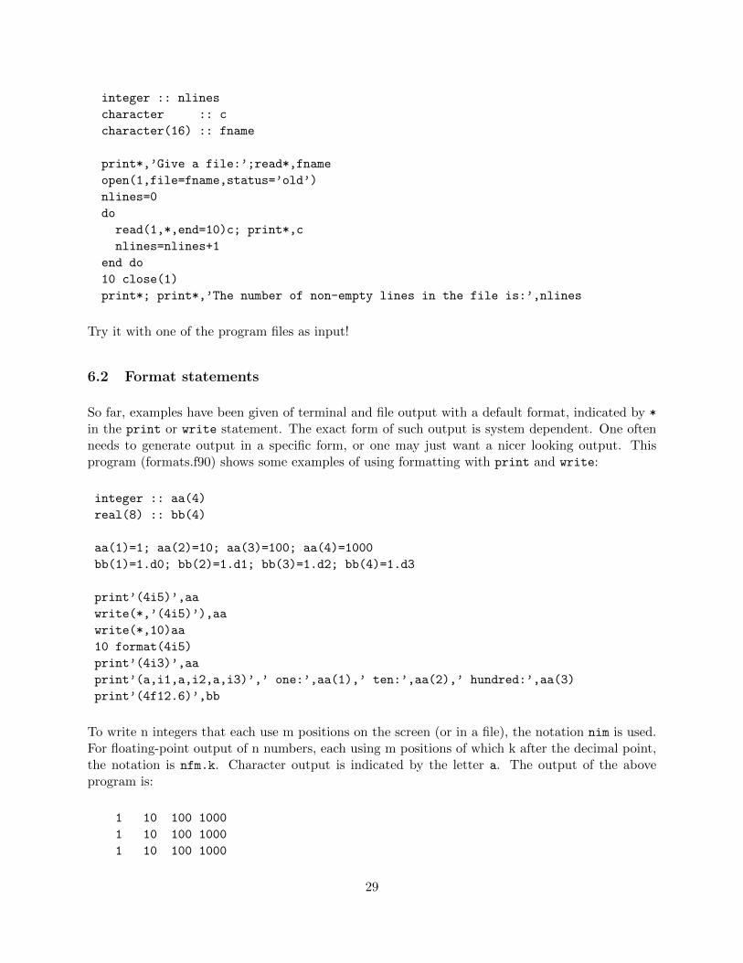
in the print or write statement. The exact form of such output is system dependent. One oftenneeds to generate output in a specific form, or one may just want a nicer looking output. Thisprogram (formats.f90) shows some examples of using formatting with print and write:

integer :: aa(4)

real(8) :: bb(4)

aa(1)=1; aa(2)=10; aa(3)=100; aa(4)=1000

bb(1)=1.d0; bb(2)=1.d1; bb(3)=1.d2; bb(4)=1.d3

print’(4i5)’,aa

write(*,’(4i5)’),aa

write(*,10)aa

10 format(4i5)

print’(4i3)’,aa

print’(a,i1,a,i2,a,i3)’,’ one:’,aa(1),’ ten:’,aa(2),’ hundred:’,aa(3)

print’(4f12.6)’,bb

To write n integers that each use m positions on the screen (or in a file), the notation nim is used.For floating-point output of n numbers, each using m positions of which k after the decimal point,the notation is nfm.k. Character output is indicated by the letter a. The output of the aboveprogram is:

1 10 100 1000

1 10 100 1000

1 10 100 1000

29

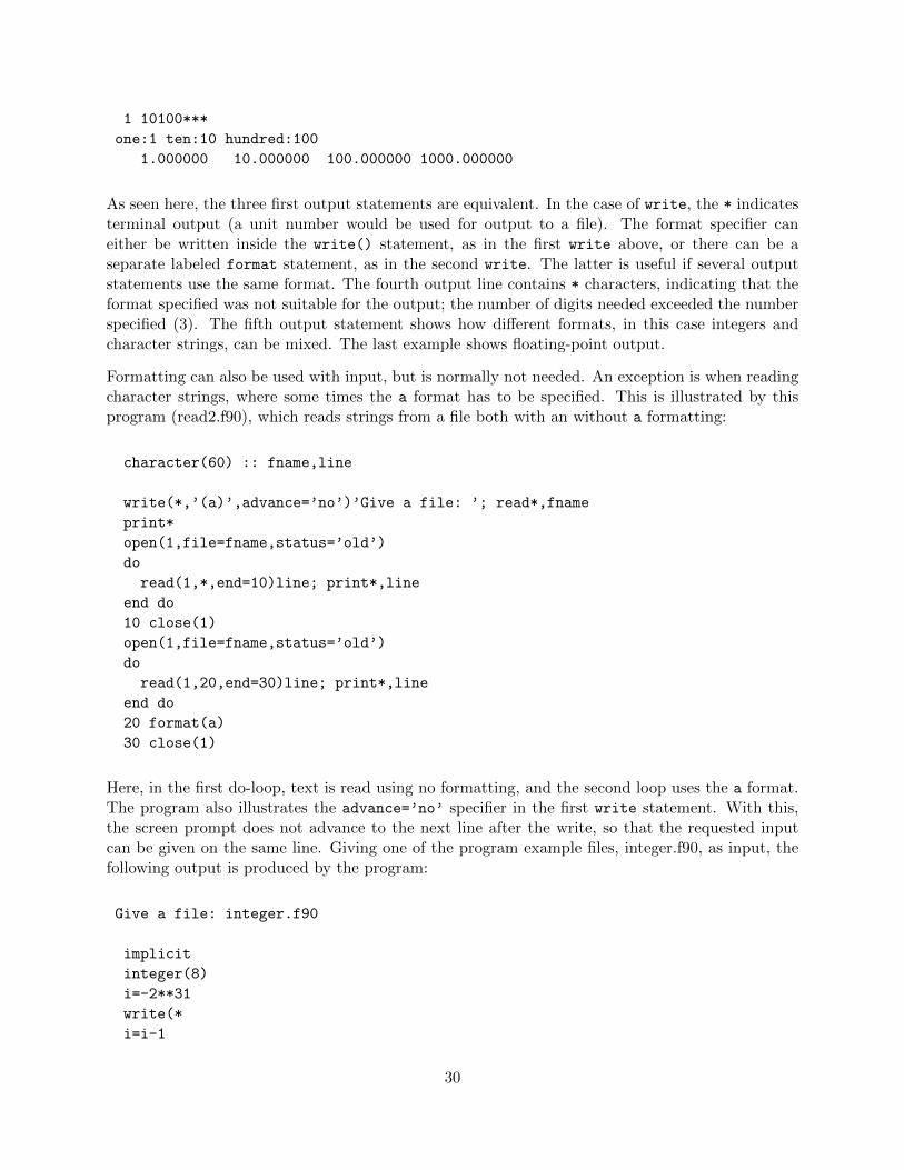
1 10100***

one:1 ten:10 hundred:100

1.000000 10.000000 100.000000 1000.000000

As seen here, the three first output statements are equivalent. In the case of write, the * indicatesterminal output (a unit number would be used for output to a file). The format specifier caneither be written inside the write() statement, as in the first write above, or there can be aseparate labeled format statement, as in the second write. The latter is useful if several outputstatements use the same format. The fourth output line contains * characters, indicating that theformat specified was not suitable for the output; the number of digits needed exceeded the numberspecified (3). The fifth output statement shows how different formats, in this case integers andcharacter strings, can be mixed. The last example shows floating-point output.

Formatting can also be used with input, but is normally not needed. An exception is when readingcharacter strings, where some times the a format has to be specified. This is illustrated by thisprogram (read2.f90), which reads strings from a file both with an without a formatting:

character(60) :: fname,line

write(*,’(a)’,advance=’no’)’Give a file: ’; read*,fname

print*

open(1,file=fname,status=’old’)

do

read(1,*,end=10)line; print*,line

end do

10 close(1)

open(1,file=fname,status=’old’)

do

read(1,20,end=30)line; print*,line

end do

20 format(a)

30 close(1)

Here, in the first do-loop, text is read using no formatting, and the second loop uses the a format.The program also illustrates the advance=’no’ specifier in the first write statement. With this,the screen prompt does not advance to the next line after the write, so that the requested inputcan be given on the same line. Giving one of the program example files, integer.f90, as input, thefollowing output is produced by the program:

Give a file: integer.f90

implicit

integer(8)

i=-2**31

write(*

i=i-1

30

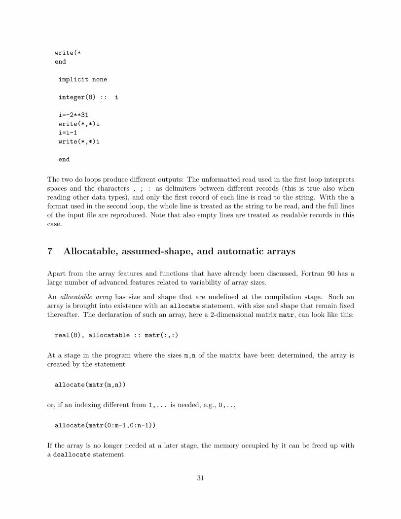
write(*

end

implicit none

integer(8) :: i

i=-2**31

write(*,*)i

i=i-1

write(*,*)i

end

The two do loops produce different outputs: The unformatted read used in the first loop interpretsspaces and the characters , ; : as delimiters between different records (this is true also whenreading other data types), and only the first record of each line is read to the string. With the a

format used in the second loop, the whole line is treated as the string to be read, and the full linesof the input file are reproduced. Note that also empty lines are treated as readable records in thiscase.

7 Allocatable, assumed-shape, and automatic arrays

Apart from the array features and functions that have already been discussed, Fortran 90 has alarge number of advanced features related to variability of array sizes.

An allocatable array has size and shape that are undefined at the compilation stage. Such anarray is brought into existence with an allocate statement, with size and shape that remain fixedthereafter. The declaration of such an array, here a 2-dimensional matrix matr, can look like this:

real(8), allocatable :: matr(:,:)

At a stage in the program where the sizes m,n of the matrix have been determined, the array iscreated by the statement

allocate(matr(m,n))

or, if an indexing different from 1,... is needed, e.g., 0,..,

allocate(matr(0:m-1,0:n-1))

If the array is no longer needed at a later stage, the memory occupied by it can be freed up witha deallocate statement.

31

Assumed-shape arrays are used as dummy arguments in procedures; they are needed when the sizeand shape of an array to be processed by the procedure can vary. In many cases, this situation canbe handled by declaring the dummy array with a variable size that is also passed as an argument, e.g,call asubroutine(matr,n) whith the matrix declared real :: matr(n,n) in the subroutine.The assumed-shape array feature is an alternative which does not require the size as an argument.The declaration in this case would be

real :: matr(:,:)

The size and shape of such an array can be obtained in the subprogram using the functions

size(array) total number of elements in the array

size(array,d) size of the array in the dimension d

shape(array) vector with elements containing the sizes in all dimensions

The use of assumed-shape arrays requires an interface declaration in the program unit calling thesubprogram. The interface is a redeclaration of the subprogram and its argument list; an examplebelow will demonstrate this.

Automatic arrays are local variables declared in subprograms using the size function of otherarrays (typically assumed-shape arrays) for their shapes.

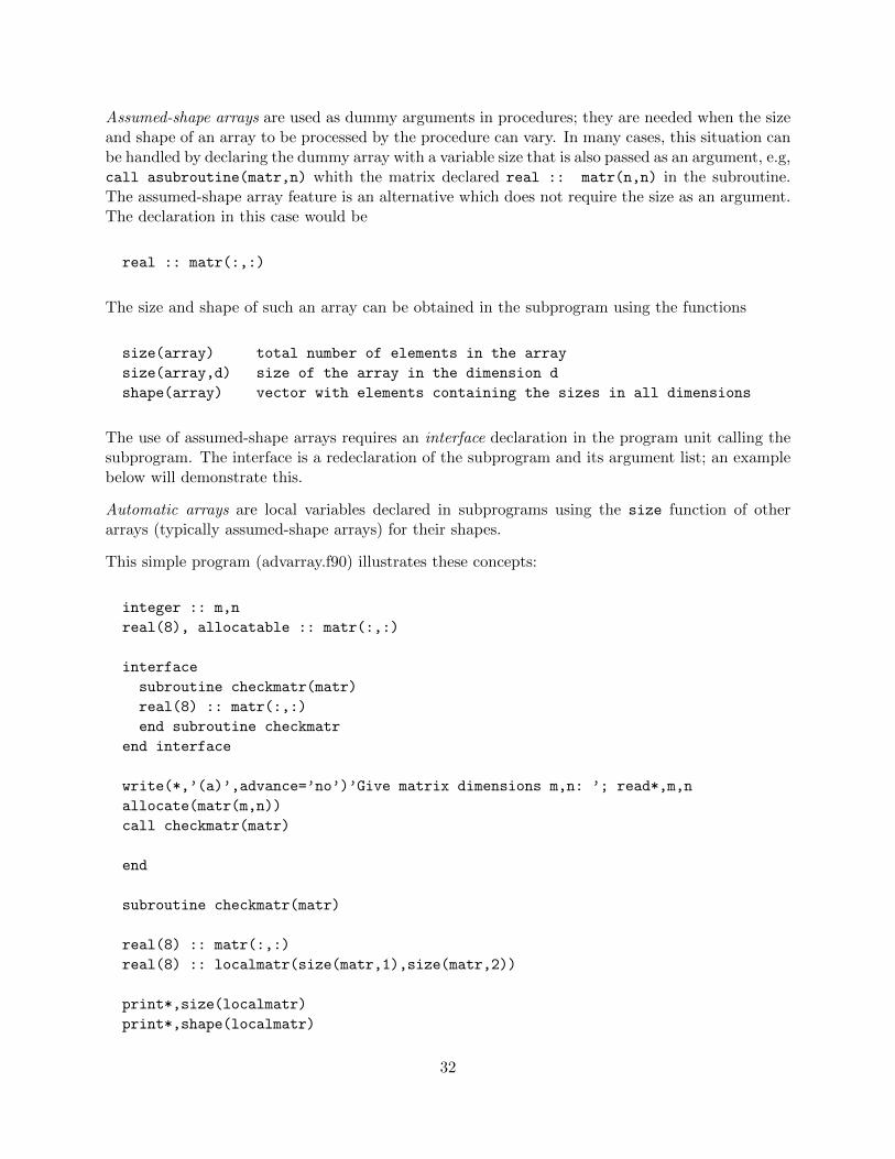
This simple program (advarray.f90) illustrates these concepts:

integer :: m,n

real(8), allocatable :: matr(:,:)

interface

subroutine checkmatr(matr)

real(8) :: matr(:,:)

end subroutine checkmatr

end interface

write(*,’(a)’,advance=’no’)’Give matrix dimensions m,n: ’; read*,m,n

allocate(matr(m,n))

call checkmatr(matr)

end

subroutine checkmatr(matr)

real(8) :: matr(:,:)

real(8) :: localmatr(size(matr,1),size(matr,2))

print*,size(localmatr)

print*,shape(localmatr)

32

end subroutine checkmatr

The interface declaration in the main program is recommended, but not required, for all externalsubprograms (we have neglected this feature so far, which is normally fine). An interface declarationis required for subprograms using assumed-shape arrays. As can be seen in the example above, aninterface contains the first and last line of the subroutine and the declarations of all its arguments(the variable names don’t have to match, only the type declarations).

The program allocates a matrix matr with shape given by the user. The subroutine checkmatr

is called with matr as an assumed-shape array. In the subroutine, another matrix, localmatr,with the same shape is declared, with dimensions obtained using the shape function (i.e., it is anautomatic array). The size and shape functions are demonstrated in the print statements of thesubroutine. Here is an example of output of this program:

Give matrix dimensions m,n: 5 6

30

5, 6

In this case, there is no deallocate statement; it can be used to free up memory when a largearray is no longer needed.

The memory occupied by local variables of a subprogram is normally freed up when the subprogramis exited (unless they are declared with the save attrivute, e.g., integer, save :: a,b, in whichcase their values are retained. If an array is allocated in a subprogram, it should be deallocatedbefore exiting the subprogram, in order to avoid potential problems with arrays that remain in anundefined state. In order to test whether an allocatable array is currently allocated or not, thelogical function allocated(array) can be used.

*********************

33