BriMon: A Sensor Network System forRailway Bridge Monitoring

Kameswari Chebrolu∗, Bhaskaran Raman∗, Nilesh Mishra+, Phani Kumar Valiveti†, Raj Kumar‡∗Indian Institute of Technology, Bombay +University of Southern California

†Cisco Systems ‡Indian Army

Abstract: Railway systems are critical in many regions,and can consist of several tens of thousands of bridges, be-ing used over several decades. It is critical to have a sys-tem to monitor the health of these bridges and report whenand where maintenance operations are needed. This paperpresents BriMon, a wireless sensor network based system forsuch monitoring. The design of BriMon is driven by two im-portant factors: application requirements, and detailed mea-surement studies of several pieces of the architecture. In com-parison with prior bridge monitoring systems and sensor net-work prototypes, our contributions are three-fold. First,wehave designed a novel event detection mechanism that triggersdata collection in response to an oncoming train. Next, Bri-Mon employs a simple yet effective multi-channel data trans-fer mechanism to transfer the collected data onto a sink lo-cated on the moving train. Third, the BriMon architecture isdesigned with careful consideration of the interaction betweenthe multiple requisite functionalities such as time synchro-nization, event detection, routing, and data transfer. Basedon a prototype implementation, this paper also presents sev-eral measurement studies to show that our design choices areindeed quite effective.

1 IntroductionRailway systems are a critical part of many a nation’s

infrastructure. For instance, Indian Railways is one of thelargest enterprises in the world. And railway bridges forma crucial part of the system. In India, there are about 120,000such bridges [1] spread over a large geographical area. 57% ofthese bridges are over 80 years old and many are in a weak anddistressed condition. It is not uncommon to hear of a majoraccident every few years due to collapse of a bridge. An auto-mated approach to keeping track of bridges’ health to learn ofany maintenance requirements is thus of utmost importance.

In this paper, we present the design ofBriMon, a systemfor long-termrailway bri dgemonitoring. Two factors guidethe design of BriMon. (1) Given the huge number of exist-ing bridges that need to be monitored, it is important that anysolution to the problem should beeasy to deploy. (2) Next,since technical expertise is both difficult to get and expensiveon field, it is equally important that the deployment requireminimal maintenance.

To facilitate ease of deployment, we choose to build our

system based on battery operatedwirelesssensor nodes. Bri-Mon consists of several tens to hundreds of such nodesequipped with accelerometers, spread over the multiple spansof the bridge. The use ofwireless transceiversand batteryeliminates the hassle of having to lay cable to route data orpower (tapped from the 25 KV overhead high voltage line ifavailable) to the various sensors that are spread about on thebridge. Cables and high voltage transformers typically needspecial considerations for handling and maintenance: safety,weather proofing, debugging cable breaks, etc.; the use ofwireless sensor nodes avoids these issues.

We also reject the possibility of using solar panels as asource of renewable energy. They are not only expensive, theyare also cumbersome to use: some sensors may be placed un-der the deck of the bridge where there is little sunlight. Fur-thermore, solar panels are also prone to theft in the mostlyunmanned bridges.

Given the choice of a battery operated wireless nodes forBriMon, a key goal which drives our design is low energy con-sumption, so that the maintenance requirements of BriMon(visits to the bridge to change battery) are kept to a minimum.

A significant challenge which arises in this context is thefollowing. The nodes need to sleep (turn off radio, sensors,etc) most of the time to conserve power. But they also need tobe ready for taking accelerometer measurements when thereis a passing train. BriMon employs a novel event detectionmechanism to balance these conflicting requirements.

Our event detection mechanism consists of a beaconingtrain and high gain external antennae at designated nodes onthe bridge that can detect the beacons much before (30s ormore) the train approaches the bridge. This large guard in-terval permits a very low duty cycle periodic sleep-wakeup-check mechanism at all the nodes. We use a combination oftheoretical modeling and experimentation to design this peri-odic wakeup mechanism optimally.

On detecting a train, BriMon nodes collect vibration data.The collected data then has to be transferred to a central lo-cation. This data will be used for analysis of the bridge’scurrent health as well as for tracking the deterioration ofthe bridge structure over time. For this, BriMon uses anapproach quite different from other sensor network deploy-ments [2, 3, 4, 5, 6, 7]. We use the passing trains themselvesfor the data transfer. The data transfer mechanism is also acti-vated through the same event detection mechanism as for datacollection.

A very significant aspect of the mobile data transfer modelis that it allows us to break-up the entire system of sensornodes (of the order of few hundred nodes) into multipleinde-pendentand much smaller networks (6-12 nodes each). Thisgreatly simplifies protocol design, achieves good scalabilityand enhances performance.

In our overall architecture, apart from event detection andmobile data transfer, two other functionalities play importantsupport roles: time synchronization and routing. Time syn-chronization is essential both for duty-cycling as well as inthe analysis of the data (correlating different sensor readingsat a given time). Routing forms the backbone of all commu-nication between the nodes. These four functionalities areallinter-dependent and interfacing them involves several designchoices as well as parameter values. We design this with care-ful consideration of the application requirements as well asmeasurement studies.

In comparison with prior work in structural monitoring [6,7, 8], our contributions are three-fold: (a) a novel event detec-tion mechanism, (b) a detailed design of mobile data transfer,and (c) the tight integration of the four required functionali-ties. While the notion of mobile data transfer itself has beenused in prior work (e.g. ZebraNet [9], DakNet [10]), its in-tegration with the rest of the bridge monitoring system, andcareful consideration of interaction among various protocolfunctionalities, are novel aspects of our work.

To validate our BriMon design, we have prototyped thevarious components of the system. In our prototype, we usethe Tmote-sky sensor nodes which have an 8MHz MSP430processor and the 802.15.4 compliant CC2420 radio, oper-ating in the 2.4GHz band. Our prototype also extensivelyuses external high-gain antennas connected to the motes [11].Although BriMon design is more or less independent of thechoice of accelerometers, it is worth noting that we use theMEMS-based ADXL 203 accelerometer in our prototype. Es-timates based on measurements using our prototype indicatethat the current design of BriMon should be deployable withmaintenance requirement only as infrequent as once in 1.5years or so (with 4 AA batteries used at each node).

Though our design has focused on railway bridges so far,we believe that the concepts behind BriMon will find appli-cability in a variety of similar scenarios such as road bridgemonitoring, air pollution monitoring, etc.

The rest of the paper is organized as follows. The nextsection provides the necessary background on bridge moni-toring and deduces the requirements for system design. Sub-sequently, Sec. 3 describes the overall BriMon architecture.Then, Sec. 4, Sec. 5, Sec. 6, and Sec. 7 present the detaileddesign of the four main modules of BriMon respectively:event detection, time synchronization, routing, and mobiledata transfer. Sec. 8 highlights our contributions vis-a-visprior work in this domain. We present further points of dis-cussion in Sec. 9 and conclude in Sec. 10.

2 Background on Bridge MonitoringIn this section, we provide a brief background on bridge

monitoring. The details presented here drive several of ourde-sign choices in the later sections. This information was gath-ered through extensive discussion with structural engineers.

General information on bridges: A common design forbridge construction is to have several spans adjoining one an-other (most railway bridges in India are constructed this way).Depending on the construction, span length can be anywherefrom 30m to about 125m. Most bridges have length in therange of a few hundred metres to a few km.

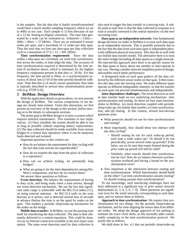
What & where to measure: Accelerometers are a com-mon choice for the purposes of monitoring the health of thebridges [6, 12]. We consider the use of 3-axis accelerometerswhich measure the fundamental and higher modal frequenciesalong the longitudinal, transverse, and vertical directions ofmotion. The placement of the sensors to capture these differ-ent modes of frequencies as well as relative motion betweenthem is as shown in Fig. 1.

Figure 1. Spans on a bridgeThe data collected by the sensors on each span are corre-

lated since they are measuring the vibration of the same physi-cal structure. In some instances of bridge design, two adjacentspans are connected to a common anchorage, in which casethe data across the two spans is correlated. For our data col-lection, we define the notion of adata-spanto consist of theset of sensor nodes whose data is correlated. A data-span thusconsists of nodes on one physical span, or in some cases, thenodes on two physical spans. An important point to note hereis that collection of vibration data across different data-spansare independent of each other i.e. they are not physically cor-related. In the rest of the paper, when not qualified, the termspan will refer to a data-span.

When, how long to collect data: When a train is on aspan, it induces what are known asforced vibrations. Afterthe train passes the bridge, the structure vibrates freely (freevibrations) with decreasing amplitude till the motion stops.Structural engineers are mostly interested in the natural andhigher order modes of this free vibration as well as the cor-responding damping ratio. Also of interest sometimes is theinduced magnitude of the forced vibrations. For both forcedas well as free vibrations, we wish to collect data for a dura-tion equivalent to about five time periods of oscillation. Thefrequency components of interest for these structures are inthe range of about 0.25 Hz to 20 Hz [6, 7, 12]. For 0.25 Hz,five time periods is equivalent to 20 seconds. The total datacollection duration is thus about 40 seconds (20 seconds eachfor forced and free vibrations).

Quantity of data: As mentioned earlier, each node col-lects accelerometer data in three different axes (x, y, z). Thesampling rate of data collection is determined by the maxi-mum frequency component of the data we are interested in:20 Hz. For this, we need to sample at least at 40 Hz. Oftenoversampling (at 400 Hz or so) is done and the samples aver-aged (on sensor node itself before transfer) to eliminate noise

in the samples. But the data that is finally stored/transmittedwould have a much smaller sampling frequency which we setto 40Hz in our case. Each sample is 12-bits (because of useof a 12 bit Analog-to-Digital converter). The total data gen-erated by a node can be estimated as: 3channels× 12bits×40Hz×40sec= 57.6Kbits. There are an estimated 6 sensornodes per span, and a maximum of 12 nodes per data span.Thus the total data we have per data-span per data collectioncycle is a maximum of 57.6×12= 691.2Kbits.

Time synchronization requirement: Since the datawithin a data-span are correlated, we need time synchroniza-tion across the nodes, to time-align the data. The accuracy oftime synchronization required is determined by the time pe-riod of oscillation above, which is minimum for the highestfrequency component present in that data i.e. 20 Hz. For thisfrequency, the time period is 50ms, so a synchronization ac-curacy of about 5ms (1/10 of the time period) should be suffi-cient. Note that this is of much coarser granularity than whatis typically described in several time synchronization proto-cols (e.g. FTSP [13]).

3 BriMon: Design OverviewWith the application details as given above, we now present

the design of BriMon. The various components of our de-sign are closely inter-related. Given this interaction, wefirstpresent an overview of the design in this section, before mov-ing on to the details in subsequent sections.

The prime goal in BriMon design is to have a system whichrequires minimal maintenance. This translates to two impli-cations. (1) Once installed, the system should be able to runas long as possible without requiring battery replacements.(2) The data collected should be made available from remotebridges to a central data repository where it can be analyzed,faults detected and isolated.

Important questions in this context are:

• How do we balance the requirement for duty cycling withthe fact that train arrivals are unpredictable?

• How do we transfer the data from the place of collectionto a repository?

• How can we achieve scaling, for potentially longbridges?

• What are going to be the inter-dependencies among Bri-Mon’s components, and how do we resolve them?

We answer these questions as follows.Event detection: We balance the requirements of having

to duty cycle, and being ready when a train arrives, throughour event detection mechanism. We use the fact that signifi-cant radio range is achievable with the 802.15.4 radios [11],on using external antennas. An 802.15.4 node on the trainbeacons as it arrives, and is detected several tens of secondsin advance (before the train is on the span) by nodes on thespan. This enables a periodic sleep/wake-up mechanism forthe nodes on the bridge.

Mobile data transfer: In BriMon, we use the passing trainitself for transferring the data collected. The data is thenulti-mately delivered to a central repository. This could be done,via say an Internet connection available at the next major trainstation. The same event detection used for datacollection is

also used to trigger the datatransferto a moving train. A sub-tle point to note here is that the data collected in response to atrain is actually conveyed to the central repository via thenextoncoming train.

Data span as an independent network:One fundamentaldesign decision we make in BriMon is to treat each data-spanas anindependentnetwork. This is possible primarily due tothe fact that the data from each data-span is independent phys-ically (different physical structures). This also fits in well withour mobile data transfer model. The alternative here is to treatthe entire bridge (including all data spans) as a single network.We rejected this approach since there is no specific reason forthe data-spans to know about one another or inter-operate inany way. Having a smaller network simplifies protocol design,and enables much better performance.

A designated node on each spangathersall the data col-lected by the different sensor nodes on that span. It then trans-fers this data onto the moving train. We make different spansoperate on different independent channels, so that the transferon each span can proceed simultaneously and independently.

Inter-dependence challenges:The event detection as wellas data transfer bank on two underlying mechanisms: timesynchronization and routing. So there are four main function-alities in BriMon: (a) event detection coupled with periodicsleep/wake-up, (b) mobile data transfer, (c) time synchroniza-tion, and (d) routing. In this context, several non-obviousquestions arise:

• What protocols should we use for time synchronizationand routing?

• More importantly, how should these two interact withany duty cycling?

– Should routing be run for each wake-up period,each time a node wakes up? Or should it be runperiodically, across several wake-up periods? If thelatter, can we be sure that routes formed during theprior wake-up period will still be valid?

– Similarly, when exactly should time synchroniza-tion be run? How do we balance between synchro-nization overhead and having a bound on the syn-chronization error?

• Also important is the interaction between routing andtime synchronization. Which functionality should buildon the other? Can time synchronization assume routing?Or should routing assume time synchronization?

To our knowledge, such interfacing challenges have notbeen addressed in a significant way in prior sensor networkdeployments [2, 3, 4, 5, 6, 7, 9]. These questions are signifi-cant even for the small networks corresponding to each data-span, and we answer them as follows.

Approach to time synchronization: We require time syn-chronization for two things: for the periodic sleep/wake-upmechanism, and for time-aligning the sensor data from differ-ent nodes. We adopt the design approach ofnot seeking toestimate the exact clock drifts, as this normally adds consid-erable complexity to the time synchronization protocol. Wejustify this as follows.

We shall show in Sec. 4.1 that our periodic sleep/wake-up

has a period of the order of 30-60s, with a wake-up duration ofabout 200ms. And we show that we can have a light-weighttime synchronization mechanism run during every wake-upduration, at no extra cost. In the time-period between twowake-up durations, of about a minute, the worst case clockdrift can be estimated. The work in [14] reported a worst-case drift of about 20ppm for the same platform as ours. Thismeans a maximum drift of 1.2ms over 60s. This is negligibleas compared to our wake-up duration, and hence exact driftestimation is unnecessary.

With respect to our application too, the time synchroniza-tion requirement is not that stringent. Recall from Sec. 2 thatwe require only about 5ms or less accuracy in synchroniza-tion. So this too does not require any drift estimation.

Our approach to time synchronization is simple and effi-cient, and is in contrast with protocols in the literature suchas FTSP [13]. FTSP seeks to estimate the clock drift, andsynchronize clocks to micro-second granularity. Due to this,it necessarily takes a long time (of the order of a few min-utes [13]). Furthermore, it is not clear how FTSP could beadapted to work in a periodic sleep/wake-up setting such asours.

Approach to routing: The first significant question whicharises here is what is the expected stability of the routing tree;that is how often this tree changes. This in turn depends onlink stability. For this, we refer to an earlier study in [11],where the authors show the following results, on the same802.15.4 radios as used in our work. (1) When we operatelinks above a certain threshold RSSI (received signal strengthindicator), they are very stable, even across days. (2) Be-low the threshold, the link performance is unpredictable oversmall as well as large time scales (few sec to few hours).

This threshold depends on the expected RSSI variability,which in turn depends on the environment. In practice, inmostly line-of-sight (LOS) environments such as ours1, oper-ating with a RSSI variability margin of about 10dB is safe.So, given that the sensitivity of the 802.15.4 receivers is about−90dBm, having an RSSI threshold of about−80dBmis safe.

With such a threshold based operation, in [11], it is ob-served that link ranges of a few hundred metres are easilyachievable with off-the-shelf external antennas. The measure-ments we later present in this paper also corroborate this. Notethat using external antennas is not an issue in BriMon since weare not particularly concerned about the form-factor of eachnode.

Now, recall that a physical span length is about 125m inthe worst case, and a data-span length can thus be about 250mmaximum. Given a link range of 100m or so, this impliesthat we have a network of at most about 3-4 hops. In suchoperation, the links will be quite stable over long durations oftime, with close to 0% packet error rate.

This then answers most of our questions with respect torouting. The protocol used can be simple, only needing todeal with occasional node failures. We need to run the rout-ing protocol only occasionally. And time synchronization caneffectively assume the presence of a routing tree, which has

1Within a span, it is reasonable to expect several pairs of nodeswith LOS between them.

remained stable since the last time the routing algorithm wasrun.

With this high level description, we now move on to thedetailed design of each of the four components of BriMon.

4 Event Detection in BriMonEvent detection forms the core of BriMon. It is needed

since it is difficult to predict when a train will cross a bridge(trains can get delayed arbitrarily). It needs to go hand-in-hand with a duty cycling mechanism for extending batterylifetime, and thus minimizing maintenance requirements.

In the description below, we first assume that the nodes aresynchronized (possibly with some error). And we assume thatwe have a routing tree, that is, each node knows its parent andits children. Once we discuss time synchronization and rout-ing, it will become apparent as to how the system bootstrapsitself. At the core of our event detection mechanism is theability to detect an oncoming train before it passes over thebridge. We seek to use the 802.15.4 radio itself for this.

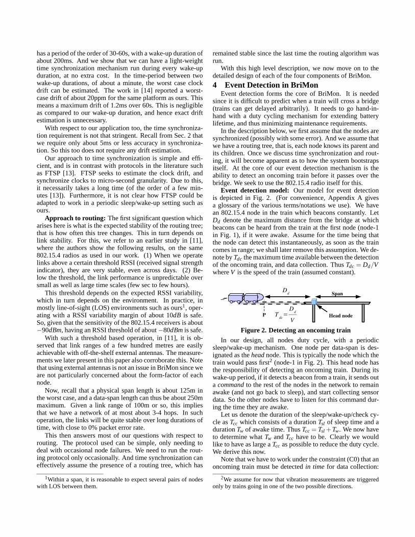
Event detection model: Our model for event detectionis depicted in Fig. 2. (For convenience, Appendix A givesa glossary of the various terms/notations we use). We havean 802.15.4 node in the train which beacons constantly. LetDd denote the maximum distance from the bridge at whichbeacons can be heard from the train at the first node (node-1in Fig. 1), if it were awake. Assume for the time being thatthe node can detect this instantaneously, as soon as the traincomes in range; we shall later remove this assumption. We de-note byTdc the maximum time available between the detectionof the oncoming train, and data collection. ThusTdc = Dd/VwhereV is the speed of the train (assumed constant).

Figure 2. Detecting an oncoming train

In our design, all nodes duty cycle, with a periodicsleep/wake-up mechanism. One node per data-span is des-ignated as theheadnode. This is typically the node which thetrain would pass first2 (node-1 in Fig. 2). This head node hasthe responsibility of detecting an oncoming train. During itswake-up period, if it detects a beacon from a train, it sends outa commandto the rest of the nodes in the network to remainawake (and not go back to sleep), and start collecting sensordata. So the other nodes have to listen for this command dur-ing the time they are awake.

Let us denote the duration of the sleep/wake-up/check cy-cle asTcc which consists of a durationTsl of sleep time and adurationTw of awake time. ThusTcc = Tsl +Tw. We now haveto determine whatTw andTcc have to be. Clearly we wouldlike to have as large aTcc as possible to reduce the duty cycle.We derive this now.

Note that we have to work under the constraint (C0) that anoncoming train must be detectedin time for data collection:

2We assume for now that vibration measurements are triggeredonly by trains going in one of the two possible directions.

all nodes must be awake and ready to collect data by the timethe train enters the data-span.

We ensure constraint C0 by using two sub-constraints.SC1: If the head node detects an oncoming train at the be-ginning of one itsTw windows (i.e. as soon as it wakes up),then it should be able to convey the command to the rest ofthe nodes within the sameTw. And SC2: there must at leastbe onefull Tw duration between the time the train is in rangeand the time data collection is due: that is, the train is betweenpoint P and the head node in Fig. 2.

Clearly, SC1 and SC2 ensure that C0 is satisfied. Now, SC1determinesTw and SC2 determinesTcc, as we explain below.

SC1 says that the windowTw should essentially be suffi-cient for the head node to be able to convey a command. De-note the time taken by the protocol for command issue asTpc.That is, within this time, all nodes in the network would havelearnt of any command issued by the head node. In additionto Tpc, Tw should also include any possible clock differencesbetween the various nodes (i.e. due to synchronization error).Let us denote byT∆ the maximum possible clock difference.

In our design, we choose to work with the worst case pos-sibleT∆, and assume that it is known. The worst caseT∆ canbe estimated for a given time synchronization mechanism.

With such an approach, the head node should wait for aduration ofT∆ before starting its command issue, to ensurethat the other nodes will be awake. Thus,Tw should at least beT∆ +Tpc. Now, from the point of view of the non-head nodesin the network,Tw should include an additionalT∆. This isbecause it could have been the case that the other nodes infact were awakeT∆ earlier than the head node. Thus we haveTw = 2T∆ +Tpc.

Using SC2, we can fix the relation:Tcc ≤ Tdc−Tw, as weexplain now. Fig. 3 argues why this condition is both neces-sary and sufficient for ensuring SC2. In the figure, we con-sider various possibilities for the occurrence of the time win-dow Tdc, with respect to the time-line at the head node.t0 isthe start of the firstTw window, before the end of whichTdcstarts. IfTdc starts (the train comes within range) at or beforet0, command issue happens during the firstTw (this is case (a)).Otherwise,Tdc starts aftert0 but beforet1, and command is-sue happens in the secondTw (this is case (b)). Clearly in bothcases, we have a fullTw window when the train is in range,and before data collection is due.

Figure 3. Train detection by head node:Tcc ≤ Tdc−Tw

Since we wantTcc to be as large as possible, we haveTcc =Tdc−Tw as the optimal value.

Incorporating detection delays: One aspect which thedescription above has not considered is the delay which wouldbe involved in detecting the train once the head node wakesup, and the train is in range. Suppose the period of the bea-

cons from the train isTb. And suppose we defineDd such thatthe packet error rate (of the beacons) from the train to the headnode is at most 20%. Then we can surely say that within 5beacon periods, the probability that the train goes undetectedis extremely small (< 10−3). So it would work in practice toset the detection delayTdet to be 5Tb.

Now, to incorporateTdet in our sleep/wake-up mechanism,we need to add the following feature: the head node has tobe awake for a durationTdet ahead of the other nodes in thenetwork. So for the head node,Tw = Tdet+T∆ +Tpc. Note thatthe non-head nodes still haveTw = 2T∆ +Tpc.

The above is the essence of our event detection mechanism.In this, we have three important parameters:Dd, Tpc, andT∆.We now describe detailed experiments to the maximum possi-ble Dd (i.e. how soon we can detect the oncoming train). Thenext section (Sec. 5) then looks at the other two important pa-rameters:Tpc, andT∆, in the context of our synchronizationmechanism.

4.1 Radio range experimentsThe distanceDd essentially captures the distance at which

beacons sent from the train can be received at the head node.Measurements in [11] indicate that if we use external anten-nas connected to 802.15.4 radios, we can achieve radio rangesof a few hundred metres in line-of-sight environments. How-ever, [11] does not consider mobile 802.15.4 radios. Hence weperformed a series of careful experiments with one stationarynode and one mobile node3.

We note that we usually have about a 1kmapproachzoneahead of a bridge. This is straight and does not have anybends. This is true for most bridges, except in hilly regions.

For our experiments too, we use a line-of-sight setting. Weused a 900m long air-strip. We mounted the stationary nodeon a mast about 3m tall. We placed the mobile node in a car,and connected it to an antenna affixed to the outside of the carat a height of about 2m. Both nodes were connected to 8dBiomni-directional antennas.

The mobile node beacons constantly, every 10ms. It startsfrom one end of the air-strip, accelerates to a designated speedand maintains that speed (within human error). The stationarynode is 100m away from the other end (so that the car can passthe stationary node at full speed, but still come to a halt beforethe air-strip ends).

For each beacon received at the receiver, we note down thesequence number and the RSSI value. We marked out pointson the air-strip every 100m, to enable us to determine wherethe sender was when a particular beacon sequence numberwas sent4. Fig. 4 shows a plot of the RSSI as a function ofthe distance of the mobile sender from the receiver.

An immediate and interesting observation to note in Fig. 4is the pattern of variation in the RSSI as we get closer to thestationary node, for all mobile speeds. Prior to the study, wedid not anticipate such a specific pattern since previous mea-

3We intentionally describe these experiments here, and not in alater section, since the results of these experiments were used to driveour design in the first place.

4We had a person sitting in the car press theuserbutton of theTmote sky whenever the car passed a 100m mark; this gives us amapping between the mote’s timestamp and its physical position.

-95

-90

-85

-80

-75

-70

-65

-60

-55

-50

-45

0 50 100 150 200 250 300 350 400 450 500

RS

SI (

dBm

)

Distance (m)

20kmph40kmph60kmph

Figure 4. RSSI vs. distance betn. sender & receiver

surement studies have not really reported any such observa-tion [15, 16, 11]. Any RSSI variations observed are generallyattributed to unpredictable environmental aspects. In ourex-periment however, the pattern is entirely predictable: these aredue to the alternating constructive & destructive interferenceof ground reflection which happens at different distances. Theexact distance at which this happens depends on the heightsof the sender/receiver from the ground. Such variations canbe eliminated by using diversity antennas, but the Tmote skyhardware does not have such a facility.

We observe from Fig. 4 that we start to receive packetswhen the mobile is as far away as 450m, and this is moreor less independent of the mobile’s speed. The RSSI mea-surements versus distance also have implications for the linkrange in the (stationary) network on the bridge. If we followa threshold-based link model, with a threshold of−80dBm,as described earlier, we can have link ranges as high as 150-200m.

For the same set of experimental runs, Fig. 5 shows plots ofthe error-rate versus distance. The error-rate is measuredovertime windows of 5 packets. To determineDd, as discussedearlier, we look for the point where the error rate falls to about20%. From Fig. 5, we find thatDd is about 400m. This too isirrespective of the mobile speed.

0

20

40

60

80

100

0 100 200 300 400 500 600

Err

or R

ate

(%)

Distance (m)

speed=20kmphspeed=60kmph

Figure 5. Error rate vs. distance betn. sender & receiver

In Fig. 5, we see that for mobile speed of 20kmph, we seesome packet errors at about 100m. This is because of the RSSIdips we explained in Fig. 4. We note that the 60kmph line does

not show such packet errors at this distance. This is becauseat this higher speed, the mobile quickly moves away from theregion of the RSSI dip. We observed similar behaviour forhigher speeds of 70kmph and 80kmph too.

During all these experiments, the transmit power at the mo-bile node was 0 dBm, the maximum possible with the CC2420chips. We also tried an experiment with an 802.11 transmit-ter, which allowed transmission at 20dBm. Now, it is possibleto detect transmissions from an 802.11 sender at an 802.15.4receiver since they operate in the same frequency (2.4GHz).For this, we can use the CCA (Clear Channel Assessment) de-tection at the 802.15.4 receiver, as explained in [17]. We usedsuch an arrangement for our experiment, and determined therange to be at least 800m. At this distance, we were limitedby the length of the air-strip, and the range is likely more than800m. In this experiment too, we saw no significant effect ofthe mobile’s speed on this range.

What this likely implies is that we can further improveDd,if we have a built-in or an external amplifier for the CC2420chip. We expect that with the use of an external amplifier atthe train’s node, we can have a range of the order of 800mor more. (Note that the additional power consumption at thetrain’s node is not a concern).

To summarize the above measurements, when the train iscoming at a speed of 80 Kmph, and withDd = 800m, we haveTdc = 36s.

4.2 Frontier nodesOne other mechanism we propose to further increaseTdc is

the use offrontier nodes. Frontier nodes are essentially nodesplaced upstream of the sensor network (upstream with respectto the direction of the train). These nodes do not participatein any data collection, but only serve to detect the oncomingtrain much earlier.

Figure 6. Using frontier nodes to increaseTdc

An example in Fig. 6 illustrates the use of frontier nodes.Tdc is effectively doubled. Note that depending on the timing,it could be the case that the head node directly learns of trainarrival, instead of the frontier node telling it.

A relevant alternative to consider here, to extend networklifetime, is to simply have additional battery installed ateachof the nodes instead of having additional infrastructure interms of a frontier node. Note however that adding a fron-tier node improves the battery life ofall nodes uniformly bydecreasing the duty cycle, and hence is likely more beneficial.

It is possible to extend the concept of frontier nodes to havemore than one frontier node to detect the oncoming train evenfurther earlier. But the incremental benefit of each frontiernode would be lesser. Further, each frontier node also addsadditional maintenance issues. In practice we expect not morethan 1-2 frontier nodes to be used.

We now move on to the issue of time synchronization.

5 Time SynchronizationThe next important aspect we look at in BriMon design

is the time synchronization. This aspect is related close tothe periodic sleep/wake-up and event detection: two of theparameters in event detection,Tpc andT∆, are both related totime synchronization, as we explain now.

There are two separate questions here:howto do time syn-chronization (i.e. the time-sync protocol), andwhenthe pro-tocol should be run. We first focus on the protocol.

5.1 How to do time synchronization?When an 802.15.4 nodeA sends a message to nodeB, it

is possible forB to synchronize its clock to that ofA. Thisis explained for the Tmote platform in [18]. Thus intuitivelyit is possible for the entire network to synchronize itself tothe head node’s clock when a message goes (possibly overmultiple hops) from the head node to the other nodes.

Now, in our commandissue from the head node (Sec. 4)too, the message exchanges involved are exactly the same: amessage has to go from the head node to the other nodes. Infact, the same protocol message sequence can be used for syn-chronization as well as for command issue. Only the contentof the messages need to be different: for synchronization wewould carry time-stamps, and for command issue, an appro-priate byte to be interpreted at the receivers. In fact, the sameset of messages can carry both contents (piggybacking onefunctionality on the other).

Our goal in designing this message sequence for time syn-chronization and/or command issue is to minimizeTpc sincethis directly translates to a lower duty cycle. We followingthe guiding principle of optimizing for the common case. Thecommon case in our setting is that packet losses are rare, dueto the stable link quality, as explained in Sec. 3.

The protocol consists of simple steps in flooding, andbuilds on the knowledge of the current routing tree (pro-vided by the routing layer). (1) The head node sends a com-mand/sync message to its children in a broadcast packet. (2)When a node receives a command/sync message, if it has chil-dren in the routing tree, it forwards it on.

We have made an important design choice above: there areno acknowledgments in the protocol. Instead, we simply usemultiple retransmissions (say, 2 or 3) for each message. Wedesign it this way for several reasons.

First, ACKs and timeouts are likely to increase the overalldelay, especially when a node has to wait for ACKs from mul-tiple children. On the other hand, the retransmissions can besent quickly. Second, since in our network we design such thatthe links are of good quality, it is appropriate to treat packetlosses as corner cases. Third, for the command message, ab-solute reliability is not necessary. If once in an odd while atrain’s vibration measurement is missed, it is alright in ourapplication. And last, as an added advantage, just sending amessage is much easier to design and implement than havingto deal with ACKs and timeouts and the resulting corner casesin the periodic sleep/wake-up mechanism.

The next design choice in the flooding is what exactly isthe MAC scheme each node follows while transmitting. Herethe choice is quite non-obvious, as we found out the hard way.We initially used the straightforward mechanism where each

node uses carrier-sensing before transmitting any message(i.e. CSMA/CA). However, we found that this did not quitework well, even in test cases involving networks of just sixnodes. We found that there were several instances where allof the retransmissions5 were getting lost, and as a result, nodesnot successfully synchronizing (or receiving commands).

There was no significant wireless channel errors, so thatcould not be the reason for the packet losses. We ruled out thepossibility of wireless hidden nodes too: such packet lossesoccurred even when all the nodes were within range of eachother. As we delved deeper into the possible reason, the an-swer surprised us: the packet losses were happening at thereceiver’s radio buffer! That is, lack of flow-control was asignificant issue.The issue of flow control

To gain an in-depth understanding of the various delaysin the system during transmission & reception, we conductedthe following experiment. We sent a sequence of packets, of apre-determined size, from one mote to the other. We had suffi-cient gap (over 100 ms) between successive packets to ensurethat no queuing delays figure in our measurements. We alsodisabled all random backoffs. We recorded time-stamps forvarious events corresponding to each packet’s transmission aswell as reception. These events, termedS1, ...,S6 at the senderandR1, ...R5 at the receiver, are listed in Tab. 1.

Table 1. Events recorded to measure various delays

For an eventSi or Ri , denote the time-stamp ast(Si) or t(Ri)respectively. Tab. 2 tabulates the various delays correspond-ing to these events. The different rows in Tab. 2 correspondto experiments with packet sizes of 44, 66, and 88 bytes (in-cluding header overheads) respectively. The delay values inthe table are the averages over several hundred packets; thevariance was small and hence we omit it. Given the averagedelay value, we then calculate the speed of SPI/radio transfer;these values are also shown in the table.

We note that the radio speed is close to the expected250Kbps at both the sender and the receiver, for all packetsizes. (It is slightly higher than 250Kbps at the senderside, because our measurement of the[t(S5)− t(S4)] delay

5We used 3 transmissions: 1 original + 2 retransmissions in ourimplementation.

Table 2. SPI, Radio delays in tx/rx

marginally underestimates the actual delay on air.) However, asignificant aspect we note is that the SPI speed at the receiveris much lower, only about 160kbps, which is much slowerthan the radio! This means that packets could queue up at theradio, before getting to the processor. To make matters worse,the CC2420 chip used in the Tmote hardware which we used,has an on-chip receive buffer of just 128 bytes [19].

Furthermore, since the time-sync packet sent by a node toits children isbroadcast, implementing filtering at the radiois not an option (the TinyOS 2.0 software we have used doesnot yet implement filtering at the radio even for unicast pack-ets). This means that all packets have to come to the micro-controller, even those not destined for this node. For instance,a node’s sibling’s broadcasts, its parent’s sibling’s broadcasts,may all reach the micro-controller! All these put togethermean that flow-control at the link layer is an issue in this plat-form.

In Tab. 2, a few other aspects we note are the following.At the sender side, the SPI bus shows slightly higher speedthan the radio; and this SPI speed increases with packet size,which suggests a fixed overhead for each such transfer. Wealso note that there is an almost constant overhead for eachpacket due to software processing: about 1.45ms at the senderside, and 0.45ms at the receiver side. The table also shows thetotal average per-packet time taken at the sender & receiver.We can see that the total delay can be as high as over 2.5 timesthe over-the-air radio delay.

The experiment above essentially means that flow-controlis required. But this is absent in a CSMA/CA based floodingmechanism. This explains the packet losses we observed. It isworth noting that other time synchronizing approaches suchasFTSP [13] have not reported such a problem with CSMA/CA,because they do not have synchronization messages sent back-to-back. In contrast, we need to send the synchronization mes-sages as quickly as possible, to minimizeTw, and thus achievevery low duty-cycling.TDMA-based flooding

The issue of flow-control arises essentially due to the use ofa radio which is faster than the processor’s (or bus’s) capabil-ities. To circumvent this issue, we use the approach of havinga TDMA-based flooding mechanism. The idea is to have thehead node come up with a schedule, based upon which eachnode in the network will transmit. The schedule ensures thatonly one node in the network transmits at a time, and that thetime-slot duration for each packet is sufficient for successfulreception (including all delays listed in Tab. 1).

The head node can embed the schedule information too inthe time-sync (or command) messages. This works as follows.As mentioned in Sec. 3, the time-sync mechanism assumes

Figure 7. Test network used for measuringTpc

that we already have a routing tree. The routing protocol willin fact ensure that the entire tree information is known at thehead. The head then computes the schedule using a depth-firsttraversal of the routing tree. For instance, in Fig. 7, one pos-sible schedule is 1, 5, 9, 10, 3, 4. Note that only non-leaveshave to transmit. Also, note that the schedule is arranged sothat each node gets to know both the synchronization infor-mation as well as its slot assignment before it has to transmitits synchronization packet.

In the above mechanism, we have consciously chosen acentralized approach. Given the size of the network we ex-pect (up to 12 nodes), the fact that the schedule is centrallycomputed and conveyed in a packet is not an issue. (In fact,the O(n) DFS computation, and having a one-byte slot infor-mation per node, can accommodate larger networks too, ofsay 100-200 nodes).Measuring Tpc

We have implemented the protocol on our Tmote sky plat-form. We used 3 retransmissions from each node, to be on thesafer side. We determine the slot size as follows. A slot needsto accommodate 3 packets. And each packet involves the timetaken for reception. The total packet size was 42 bytes, whichhas a total delay at the receiver, of about 4ms. So we used aslot time of 12ms. This resulted in negligible packet losses.

A slot time of 12ms givesTpc = 12× 6 = 72ms, for thetest network of 12 nodes shown in Fig. 7. This is because,in this network, the six non-leaf nodes need to transmit oneafter the other. We observed this value ofTpc experimentallytoo, in our prototype implementation. Recall that we expecta data-span to have at most 12 nodes, and not more than 3-4hops. Our test network is designed to resemble a data-spanwith two physical spans. In the test, all of the 12 nodes wereplaced within range of each other, but we artificially imposeda routing tree on them. For a six-node network, we can expectTpc to be much lesser, about 36ms.

5.2 When to do time synchronization?We now turn to the question ofwhenwe should run the

above time-sync/command protocol. The command to collectdata is issued only when a train is detected. With respect to thesynchronization protocol, there is the question of how oftenwe should synchronize. For our CC2420 platform, the answer

is simple. We just run the synchronization mechanism duringeach wake-up period. This does not incur any additional over-head since anyway all nodes are awake forTw = T∆ + Tpc, inexpectation of a potential command from the head node. Andif nodes are awake and listening, the power consumption inthe CC2420 chips is the same as (in fact slightly higher than)that of transmitting [20].

We can now estimateT∆ too. It is the sum of the possi-ble clock drift in one check cycle (Tcc), andTerr, the error inthe synchronization mechanism. We estimatedTdc = 36s inSec. 4.1. SinceTcc < Tdc, the worst caseTdri f t can be esti-mated as 20× 10−6 × 36s = 0.72ms. Here we have used aworst case clock drift rate of 20ppm [14].

In the same experiment above, where we estimatedTpc, wealso measured the worst case error in our synchronization tobe at most 5-6 clock ticks over the 3-hop, 12-node network.This is about 6× 30.5µs≃ 0.18ms. The overallT∆ is thusabout 0.9ms. It is worth noting that this is much smaller thanTpc.

In our prototype implementation, we have also tested (in-lab) that the time-sync and periodic sleep/wake-up mecha-nism indeed work stably: we have tested for several hours(close to 1 day) at a stretch.

6 RoutingWe have noted above that both the event detection (com-

mand) mechanism and the time-sync protocol depend on theexistence of a routing tree rooted at the head node. The cruxof our routing mechanism is the fact that we use stable links.That is, unlike in [16], we do not have a situation where wehave to distinguish between links of error rates in-between0% and 100%. In fact, the RSSI and LQI variability measure-ments in [11] suggest that trying to make such distinctions ina dynamically varying metric can produce unstable behaviour(in the 802.15.4 platform).

Routing phases: In designing the routing, we make thedesign decision of using a centralized routing approach, withthe head node controlling decisions. We have the followingsimple steps in routing. (1)Neighbour-discovery phase:Thehead node initiates this phase, by periodically transmittinga HELLO. Nodes which hear the HELLO in turn periodi-cally transmit a HELLO themselves. After some time, eachnode learns the average RSSI with its neighbours, which weterm the link-state. (2)Tree construction phase:The headnode now starts constructing the routing tree. The construc-tion goes through several stages, with each stage expandingthe tree by one hop. To begin with, the root node knows itsown link-state, using which it can decide its one-hop neigh-bours. Now it conveys to each of these chosen one-hop neigh-bours that they are part of the network. It also queries eachof them for their link-state. Once it learns their link-state, itnow has enough information to form the next hop in the net-work. And this process repeats until all possible nodes havebeen included in the network. In each link-state, based on theRSSI threshold, as described in Sec. 3, links are classified asgood or bad. The root first seeks to extend the network usinggood links only. If this were not possible, it seeks to extendthe network using bad links.

Although simple, the above mechanism has two properties

essential for us. (1) The head nodeknows the routing treeat the end of the two phases. This is essential for our timesynchronization and command mechanisms (e.g. to send acommand to the nodes in the network to start collecting data,after detecting an oncoming train). It is also essential whenit is time for the head node to gather all data from the nodesin the network, before transferring it to the train. (2) Moreimportantly, the head nodeknows when the routing protocolhas ended operation. We stress that this is a property notpresent in any distributed routing protocol in the literature, toour knowledge. And this property is very essential for powerefficient operation: once the head node knows that routing hasended, it can then initiate duty cycling in the network. Suchinterfacing between routing and duty cycling is, we believe,an aspect which has not really been looked at in-depth in priorwork.

When to run the routing protocol? Like with the time-sync protocol, we also need to answer the question ofwhento run the routing protocol. The routing protocol can be runinfrequently, or whenever a failure is detected. Now, how todetect failures in the network? A node can detect itself to bedisconnected from the current routing tree, if it fails to receivethe time synchronization messages for a certain timeout. Itcan then cease its duty cycling, and announce that it has beenorphaned. This announcement, if heard by a node connectedto the routing tree, is passed on to the head node. The headnode can then initiate the above routing protocol again.

We wish to stress that such a laid-back approach to fixingfailures is possible because we are relying upon stable links.We also once again stress that scaling is not an issue since weconsider each data-span to be an independent network.

In order to build tolerance to failure of the head node, onecan provision an extra head node. An alternative would be tohave one of the other nodes detect the head node’s failure (say,on failure to receive synchronization messages for a certaintimeout period), and take-over the head’s functionality.

Benefits of a centralized approach: A centralized ap-proach has several benefits, apart from the simplicity in de-sign and implementation. For example, recall from Sec. 5 thatTpc is proportional to the number of non-leaf nodes in the net-work. So we need to minimize the number of non-leaf nodes.A centralized routing approach can optimize this much moreeasily as compared to a distributed approach. Similarly, anyload balancing based on the available power at the nodes isalso more easily done in a centralized routing approach.

Routing protocol delay: Since we expect to run the rout-ing protocol only infrequently, the delay it incurs is not thatcrucial. But all the same, we wish to note that in our proto-type implementation, the routing phases take only about 1-2s,for the test network shown in Fig 7. This is much smallercompared to say, the duration of data collection (40s) or datatransfer (Sec. 7).

7 Mobile Data TransferWe now discuss the last important component of BriMon.

The event detection mechanism triggers data collection at thenodes. After the datacollectionphase, this data must reliablybe transferredfrom the (remote) bridge location to a centralserver that can evaluate the health of the bridge. Most sen-

sor network deployments today do this by firstgatheringallcollected data to a sink node in the network. The data is thentransferred using some wide-area connectivity technologytoa central server [2, 3, 4, 5, 6, 7].

We reject this approach for several reasons. First, in a set-ting where the bridges are spread over a large geographicalregion (e.g. in India), expecting wide area network coveragesuch as GPRS at the bridge location to transfer data will notbe a valid assumption. Setting up other long-distance wirelesslinks (like 802.11 or 802.16) involves careful network plan-ning (setting up towers for line of sight operation, ensuring nointerference, etc.) and adds further to maintenance overhead.Having a satellite connection for each bridge is too expensivea proposition. Manual collection of data via period trips tothebridge also means additional maintenance issues.

A more important reason is the following. Recall that wecan have bridges as long as 2km, with spans of length 30-125m. This means that overall we could have as many asabout 200 sensors placed on the bridge, at different spans.Even if we were to have somehow have a long-distance In-ternet link at the bridge location, we would have togatherallthe sensor data corresponding to these many sensors at a com-mon sink, which has the external connectivity. Such gatheringhas to be reliable as well.

The total data which has to be gathered would be substan-tial: 57.6Kb× 200≃ 1.44MB for each measurement cycle.Doing such data gathering over 10-20 hops will involve ahuge amount of transfer time and hence considerable energywastage. Having a large network has other scaling issues aswell: scaling of the routing, synchronization, periodic wake-up, command, etc.. Large networks are also more likely tohave more fault-tolerance related issues.

Keeping the above two considerations in mind, we con-sider a mobile data transfer mechanism, where data from themotes is transferred directly to the train. This then allowsusto partition up the entire bridge into several data-spans withindependently operating networks. In each data-span, the des-ignated head node gathers data from all the nodes within thedata-span. It then transfers the data gathered for the data-spanonto the train. Since we are dealing with networks of sizeat most 12 nodes, data gathering time is small, and so is thetransfer time to the train itself. We eliminate the need for aback-haul network in such an approach.

One subtle detail to note here is that we seek to transfer thedata collected for one particular train, not to the same train,but to a subsequent train. In fact on the Tmote platform, itis not possible to use the radio in parallel with the data col-lected being written to the flash since there is a common bus.We then need to have different trains for data collection andthe data transfer. The additional delay introduced in such anapproach is immaterial for our application.

The transport protocol itself for the data transfer can bequite simple. In BriMon, we use a block transfer protocolwith NACKs for the data transfer from the head node to thetrain. We use a similar protocol, implemented in a hop-by-hopfashion, for the data gathering as well: that is, for gettingthedata from the individual nodes to the head node.

There are a few challenges however in realizing our mobiledata transfer model. One, while one cluster head is transmit-

ting data of its cluster to the train, nearby cluster heads wouldalso be within contact range of the train and would be trans-ferring their data. This would lead to interference if sufficientcare is not taken. In fact, the synchronization, routing, andother operations of multiple spans could interfere with onean-other. We can address this issue by using multiple channels,as we explain below.

Using multiple channels: We take the approach of usingthe 16 channels available in 802.15.4. There are at least eightindependent channels available [14]. We could simply use dif-ferent channels on successive spans, and repeat the channelsin a cycle. For instance we could use the cycle 1, 3, 5, 7, 9,11, 13, 15, 2, 4, 6, 8, 10, 12, 14, 16. This would ensure thatadjacent channels are at least 7 spans apart, and independentoperation of each data-span would be ensured. Note that thetrain needs to have different motes, operating in the appropri-ate channel, for collecting data from each data-span.

Reserved channel for event detection:The above ap-proach works except for another subtle detail. We desig-nate that the channel for event detection mechanism for alldata-spans is the same, and reserve one channel for this pur-pose. So as the train approaches, the radio within it can con-tinuously beacon on this reserved channel without having tobother about interfering with any data transfer or other proto-col operation within each data span. The head nodes of eachspan listen on this channel for the oncoming train, and switchto the allocated channel for the data-span after theTdet dura-tion6.

Throughput issues: Another challenge to address in ourmobile data transfer mechanism is whether such transfer ispossible with sufficient throughput. The amount of data thatcan be transferred is a function of the contact duration of thetrain with the mote, which in turn is a function of the speed ofthe train and the antennae in use.

In order to determine the amount of data that can be trans-ferred using our hardware platform, we have conducted exper-iments with a prototype. We have implemented the NACK-based reliable block transfer protocol. Although simple con-ceptually, the protocol involves some subtleties in implemen-tation. We need to transfer blocks of data from the flash ofthe sender to the flash of the receiver. As mentioned earlier,in the Tmote platform, we cannot perform flash read/write si-multaneously with radio send/receive because of a shared bus.However, our protocol does parallelize flash write at the re-ceiver, with flash read of the next block at the sender.

In our implementation, we use blocks of size 2240 bytes;this is significant chunk of the 10KB RAM in the MSP430chip of Tmote sky. And we have used packets of payload116 bytes. So a block fits in 20 packets. In our data transfermechanism, the sender simply uses apausebetween succes-sive packets to implement flow control. We compute the pauseduration as the excess total delay at the receiver side as com-pared to the sender side. Using an extrapolation of Tab. 2, wecalculate the required pause duration for packets of payload116 bytes (total 126 bytes) to be about 3ms (sender side de-lay: 8ms, receiver side delay: 11ms). We use a value of 4ms,

6Such channel change takes only a few hundred micro-sec on theCC2420 chips.

as a safety margin.To get an estimate of the various delays involved in the

protocol, we first ran a data transfer experiment using an over-all file size of 18 blocks. The total time taken was 6,926ms.This consists of the following components. (1) A flash read-time for each block of about 100ms. (2) A flash write-timefor each block of about 70ms. This is overlapped with theflash read-time for the next block, except of course for the lastblock. (3) The transmission + pause time for each packet isabout 12, resulting in an overall transmission + pause timeof 20× 12 = 240ms per block. So we expect a delay of18× 100ms+ 1× 70ms+ 18× 240ms= 6190ms, which isclose to the experimentally observed delay of 6,926ms.

The above experiment thus gives an effective throughputof 2,240×18×8/6926= 46.6Kbps. Note that this value ismuch lower than the 250Kbpsallowed by the 802.15.4 radio,due to the various inefficiencies: (a) various header overheads,(b) the shared bus bottleneck mentioned above due to whichflash read/write cannot be in parallel with radio operation,and(c) the use of a pause timer to address the flow-control issue.

Mobile data transfer experiment: To see if we are ableto achieve similar throughput under a realistic scenario, weconducted the following experiment. The setup mimics thesituation where the header node (root node) of a cluster inBriMon uploads the total data collected by all the nodes withinits cluster on to mobile node on a train. The data transfer isinitiated when the mobile node (on the arriving train) requeststhe head node to transfer the collected data. The head nodethen reads the data stored as files from flash and uploads themone by one using the reliable transport protocol.

In this experiment, the head node was made to transfer 18blocks of data, each of 2240 bytes. The total data transfer wasthus 18×2240= 40,320B. The head node as well as mobilenode were equipped with external 8dBi omni antennas, muchlike in Sec. 4.1. The antenna of the head node was mountedat a height slightly over 2m. The mobile node was fixed on avehicle and the antenna was at an effective height of slightlyless than 2m.

The head node (stationary) with the complete data of40,320B in its flash, is initially idle. The mobile node is turnedoff until it is taken out of the expected range from the headnode, and then turned on. The experiments in Sec. 4.1 showthat the range can be around 400m. So we started the mo-bile node at a distance of 500m from root node. The vehicle ismade to attain a constant known velocity at this point of 500m,while coming towards the head node. On booting, the mobilenode starts sending the request for data, every 100ms, untilit receives a response from the head node. The head node,on receiving the request, uploads the data block by block, us-ing the reliable transport protocol. The transport layer atbothnodes takes a log of events like requests, ACKs, NACKs andretransmissions, for later analysis.

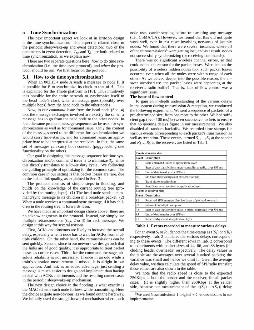
Fig. 8 shows a plot of the block sequence number receivedat the mobile node, versus the position of the mobile with re-spect to the head node. We first note that although we con-servatively estimated the contact range to be 400m, the datatransfer begins right at about 490m, irrespective of the mo-bile’s speed. We next note that after the mobile is within 450mfrom the head node, the rate of data transfer (slope of the line)

0

2

4

6

8

10

12

14

16

18

-520 -500 -480 -460 -440 -420 -400 -380 -360

Blo

ck n

um. r

ecd.

at h

ead

node

Posn. of mobile with respect to the head node (m)

30kmph50kmph60kmph

Figure 8. Mobile data transfer measurement

is more or less constant. We have calculated this slope to cor-respond to the same data rate (about 46Kbps) as in the sta-tionary throughput test. The regions in each graph where theslope is different from this rate correspond to instances wherea NACK was sent since some of the packets in a block werelost.

Feasibility of mobile data transfer: Assuming thethroughput of about 46Kbps which we have been able toachieve, it means that if we have 691.2Kb per data-span, asestimated in Sec. 2, we need a contact duration of 691.2/46≃15s. This is achievable with a contact range of about 330mfor a train speed of up to 80kmph. Or, with a contact range ofabout 250m for a train speed of 60kmph.

Note from our discussions in Sec. 4 that in the worst case,the head node detects the oncoming train only just before thetrain passes over the span. Combining this observation withthe fact that data transfer starts right from about 490m (Fig. 8),we have sufficient contact range, larger than the 330m require-ment estimated above. So we can conclude that our data trans-fer is achievable, with significant leeway. Our analysis abovehas in fact been a worst-case analysis. For instance, the lee-way would be much higher if we have only a 6-node network,or if we use frontier nodes.

There are also other possibilities to further improve the ef-fective data transfer throughput. One obvious performanceenhancement is the use of data compression. Another possi-bility is use different hardware. We could use a mote whichallows simultaneous operation of the flash and the radio. Orwe could even use a completely different radio, say for ex-ample the Bluetooth enabled Intel motes, as considered in [5].These possibilities could give higher throughput than whatwehave been able to achieve with 802.15.4 in our prototype.

Another possibility to increase the effective amount of datawhich can be transferred to a train is to employ the followingtrick. We could have one data transfer to a receiver in the frontcoach of the train, and another in a rear coach sufficiently farapart from the front coach. This is feasible since trains areoften about 1km or more long.

8 Related WorkPrior to BriMon, several projects have looked at the issue

of automated structural health monitoring. The work in [21,7]uses MEMS-based sensors and Mica2/MicaZ motes to studyvibrations in buildings. It focuses on data compression tech-

niques, reliable data transfer protocol, and time synchroniza-tion. The work in [6, 8] has looked at bridge monitoring in-depth. They have presented extensive studies of hardware, therequired data sampling rate, and data analysis.

BriMon builds on this body of prior work in structuralmonitoring, and the techniques of data compression, datatransfer protocol, data analysis, etc are complementary toourcontributions. The novel aspects in our work are the event de-tection, mobile data transfer, as well as the integration oftheseaspects with low duty cycling. These have not been consid-ered in earlier work.

Low duty cycling by itself is not novel by any means.B-MAC [22], SCP-MAC [20] and AppSleep [23] are MACprotocols to achieve low duty cycling. Since these protocolshave been designed without anyspecificapplication in mind,they are necessarily generic. For instance, SCP-MAC usescomplex schedule exchange mechanisms with neighbouringnodes. This is designed for an arbitrary traffic pattern, andhence does not apply (optimally) in our setting.

Similarly, mobile data transfer too is not novel by itself.The ZebraNet [9] and DakNet [10] projects too have usedsimilar strategies. There is a growing body of literature inthiscontext for 802.11 (WiFi) [24, 25]. With respect to 802.15.4too, [26] presents some preliminary measurements indicatingthat mobile data transfer in 802.15.4 is feasible, and that thethroughput is independent of the speed. Our measurements inSec. 4.1 are in broad agreement with these.

In contrast to the above work on low duty cycling or mo-bile data transfer, our primary goal is to integrate the requi-site functionalities for a specific application. BriMon inte-grates vertically withall aspects relevant to bridge monitor-ing. It usesonly the necessary set of mechanisms, thus sim-plifying the design. We use extensive application informationand cross-layer optimizations across the four functionalitiesof event detection, mobile data transfer, time synchronization,and routing. To our knowledge, we are the first to have care-fully looked at the interaction between such network protocolfunctionalities.

9 DiscussionWe now present several points of discussion around the

system design described so far.Lifetime estimation: It is useful to get an idea of how

well the system we have designed is able to achieve our goalof minimal maintenance. For this, we estimate the time forwhich a set of batteries will last, before requiring replacement.Consider the sequence of events depicted in Fig. 9. We havea data collection phase, followed by a data gathering phase(data goes from each node to the head node). Then when thenext train arrives, the data is transferred to the moving train.

Figure 9. Estimating node lifetime in BriMon

We assume that we use a battery, or a series of batteries ofsufficient voltage, say 6V (at least 3V required for the Tmote

sky motes, and at least 5V for the accelerometers). For ex-ample, this can be achieved by using 4 AA batteries in series.The various current values shown are rough estimates derivedfrom the data specification sheets of the accelerometer andTmote sky respectively. We also verified many of these val-ues using a multimeter in our lab.

In Fig. 9, we can estimateTcoll , Tgather, andTtrans f er as fol-lows. Tcoll starts when the train is detected and extends until20 sec after it has crossed the span. Hence it depends on whenexactly the train is detected, train speed, the train’s length, andthe span length. Assuming the worst case when the train is de-tected very early (Tdc before it enters the span), and assumingtrain speed to be 60kmph, train length to be 1km, and data-span length to be 250m, we have:

Tcoll = 36s+(250m+1km)/(60kmph)+20= 131sWe assume that once collected, the data is truncated to only

the last 40s of data (which is of interest).Then we estimateTgather to be the time it takes for this

data to be gathered at the head node. Now, pushing 40sworth of collected data over one hop toward the root takes57.6Kb/46Kbps= 1.25s. In Fig. 7, there is one head node,4 nodes one-hop away, 5 nodes two-hops away, and 2 nodesthree-hops away. Thus if we transfer the collected data hop-by-hop, one after another, the total time taken would for thiswould be(1×0+4×1+5×2+2×3)×1.25s= 32.5s. ForTtrans f er, we use the value of 15s, as estimated in Sec. 7.

Now, usingTw = Tpc+2T∆ +Tdet will work for both headnodes as well as non-head nodes (see Sec. 4). Recall thatTpc = 72ms (for a 12-node network),T∆ ≃ 1ms, andTdet =5Tb = 50msfor an inter-beacon period ofTb = 10ms. We takeTw = 125msas an upper bound on the above estimate.

Assuming that we have data collection once per day7.There are thus at most 1day/Tcc ≃ 2400 durations ofTw andTsl. So the total energy drawn, expressed inmA× sec, at 6V,can be estimated as:

Tcoll ×50mA+Tgather×20mA+Ttrans f er×20mA+2400×Tw×20mA+2400×Tsl ×10µA= 6550 (collect) + 650 (gather) + 300 (trans f er) +6000(wakeup)+864(sleep)mAsec= 14364mAsec≃ 4mAh

The AA batteries have about 2500mAh capacity. Hencewe can expect that the lifetime in this setting would be about2500/4≃ 625days, which is over 1.5 years.

We note that in the above equation, the main componentsto the overall energy consumption are the data collection andthe periodic wake-up. In fact, if we have further infrequentdata collection, say once a week, in the above estimation theperiodic wake-up will constitute an even larger fraction ofthepower consumption. So it was indeed useful that we sought tominimize the wake-up duration in our design!

Measurements on a bridge:Most of the experiments wehave presented above have used an air-strip (or have been per-formed in lab). This was convenient since the air-strip wasnearby. However, we also tested our prototype on a road

7Measuring once a day is sufficient for long-term bridge healthmonitoring. Also note that we need not collect data for every passingtrain; we can easily build logic to look only for trains with certain idsin their beacons.

bridge on a nearby river8. We had two ADXL 203 accelerom-eter modules integrated into our system at that time. Prior toour trip to the bridge, we thoroughly tested the accelerometermodules in-lab, using calibrated shake-tables. At the bridge,we used two motes for data collection, and a separate sink(head) node.

We were successfully able to measure the vibrations on thebridge induced due to passing traffic. We observed a domi-nant free vibration frequency of about 5.5Hz. The amplitudeof forced vibration we observed was as high as 100 milli g(vertical). For healthy bridge spans, the expected amplitude isabout 30 milli g. So our measurement indicates the need formaintenance operations on that span.

The above measurement on the bridge, as well as the pro-totype implementations of the various functional components,gives us a measure of confidence in the overall design.

Wider applicability: We have designed BriMon specif-ically for railway bridge monitoring. This environment isparticularly challenging since most bridges are away froman urban environment (poor wide area network connectivity).More importantly, train traffic is sporadic and unpredictable.On the other hand, road bridges are likely to have constantand/or predictable (time-of-day related) traffic patterns. How-ever, even in such scenarios, we believe that many of ourmechanisms are likely to find applicability. For instance, weuse our event detection mechanism to trigger data transfer,toa designated mobile node. This would be applicable in roadbridges too. Also applicable would be the consideration ofmultiple channels, splitting up the set of nodes into multipleindependent networks, and the resulting architecture withthetime synchronization and routing functionalities integrated.

Apart from structural monitoring, our event triggering anddata transfer approaches are also likely to find applicability in,say road-side pollution monitoring. MEMS-based sensors arecurrently still evolving in this domain [27].

Ongoing and future work: Admittedly, many aspects ofour work require further consideration. While the prototypeimplementation and detailed experimentation have given usameasure of confidence in our design, actual deployment ona railway bridge is likely to reveal further issues. Relatedtothe issue of fault-tolerance, while we have outlined a possibleapproach to deal with head node (see Sec. 6), we have leftoptimizations in this regard for future consideration.

On application specific versus generic design:BriMonis a case study in application specific design. We have con-sciously taken this approach. Our methodology has been tostart from scratch, and pay full attention to the application re-quirements, and design the required mechanisms. And impor-tantly, we designonly the required mechanisms, thus keepingthe design relatively simple and, arguably, optimal.

Literature in protocol design for sensor networks is abun-dant. We have not tried to retro-fit any protocol designed ina generic fashion into BriMon. Our approaches to time syn-chronization and routing are two cases in point.

Although we have not sought to generalize our solutions atthis stage, this is not to say that generality is impractical. But

8The logistics for doing the same on a railway bridge are moreinvolved.

we believe that in complex systems, generality emerges fromin-depth studies of specific systems.

On layered versus integrated design:Along the samevein as above, we have also paid little heed to traditional pro-tocol layering. Cross layer interactions are well known inwireless systems in general. We have intentionally taken anintegrated approach. Once again, this is not to devalue thebenefits of layering. But we believe that the right protocol lay-ering and interfacing will emerge from specific in-depth sen-sor network system designs such as ours. Hence we have nottried to retro-fit the layering which currently exists for wirednetworks, in our system.

10 ConclusionThis paper presents the design of BriMon, a wireless sen-

sor network based system for long term health monitoring ofrailway bridges. The paradigm we have followed is that ofapplication specific design. We believe that this is the rightway to understand the complex interaction of protocols in thisdomain.

In the design of BriMon, we identify the requisite set offunctionalities from the application’s perspective, and we pro-pose mechanisms to achieve these. We build on several as-pects of prior work in automated structural monitoring. Ournovel contributions are three fold: (1) an event detectionmechanism which enables low duty cycling, (2) a mobiledata transfer mechanism, and (3) the interfacing of these twomechanisms with the time synchronization and routing func-tionalities.

Our design choices have been based on application require-ments as well as on several measurement studies using proto-type implementations. Based on preliminary measurements,we estimate that our current design should be deployable withminimum maintenance requirements: with the battery lastingfor over 1.5 years.

11 References[1] George Iype. Weak, distressed, accident-prone.http:

//www.rediff.com/news/2001/jun/25spec.htm, 25Jun 2001. The Rediff Special.

[2] Alan Mainwaring, Joseph Polastre, Robert Szewczyk,David Culler, and John Anderson. Wireless Sensor Net-works for Habitat Monitoring. InACM InternationalWorkshop on Wireless Sensor Networks and Applica-tions (WSNA), 2002.

[3] Gilman Tolle, Joseph Polastre, Robert Szewczyk, DavidCuller, Neil Turner, Kevin Tu, Stephen Burgess, ToddDawson, Phil Buonadonna, David Gay, and Wei Hong.A Macroscope in the Redwoods. InSenSys, Nov 2005.

[4] Geoffrey Werner-Allen, Konrad Lorincz, Matt Welsh,Omar Marcillo, Jeff Johnson, Mario Ruiz, and JonathanLees. Deploying a Wireless Sensor Network on an Ac-tive Volcano.IEEE Internet Computing, Mar/Apr 2006.

[5] Lakshman Krishnamurthy, Robert Adler, Phil Buon-adonna, Jasmeet Chhabra, Mick Flanigan, NandakishoreKushalnagar, Lama Nachman, and Mark Yarvis. Designand Deployment of Industrial Sensor Networks: Experi-

ences from a Semiconductor Plant and the North Sea. InSenSys, Nov 2005.

[6] Sukun Kim. Wireless Sensor Networks for StructuralHealth Monitoring. Master’s thesis, U.C.Berkeley, 2005.

[7] Jeongyeup Paek, Krishna Chintalapudi, John Cafferey,Ramesh Govindan, and Sami Masri. A Wireless SensorNetwork for Structural Health Monitoring: Performanceand Experience. InEmNetS-II, May 2005.

[8] Manuel E. Ruiz-Sandoval.Smart Sensors for Civil In-frastructure Systems. PhD thesis, University of NotreDame, Indiana, 2004.

[9] Pei Zhang, Christopher M. Sadler, Stephen A. Lyon, andMargaret Martonosi. Hardware Design Experiences inZebraNet. InSenSys, Nov 2004.

[10] Alex Pentland, Richard Fletcher, and Amir Hasson.DakNet: Rethinking Connectivity in Developing Na-tions. IEEE Computer, Jan 2004.

[11] Bhaskaran Raman, Kameswari Chebrolu, Naveen Mad-abhushi, Dattatraya Y Gokhale, Phani K Valiveti,and Dheeraj Jain. Implications of Link Range and(In)Stability on Sensor Network Architecture. InWiN-TECH, Sep 2006.

[12] Exploration of Sensor Network Field deployment on alarge Highway Bridge and condition assessment.http://healthmonitoring.ucsd.edu/documentation/public/Vincent_Thomas_Testing.pdf.

[13] Miklos Maroti, Branislav Kusy, Gyula Simon, and AkosLedeczi. The Flooding Time Synchronization Protocol.In SenSys, 2004.

[14] Hoi-Sheung Wilson So, Giang Nguyen, and Jean Wal-rand. Practical Synchronization Techniques for Multi-Channel MAC. InMOBICOM, Sep 2006.

[15] Jerry Zhao and Ramesh Govindan. UnderstandingPacket Delivery Performance in Dense Wireless SensorNetworks. InSenSys, Nov 2003.

[16] Alec Woo, Terence Tong, and David Culler. Taming theUnderlying Challenges of Reliable Multihop Routing inSensor Networks. InSenSys, Nov 2003.

[17] Nilesh Mishra, Kameswari Chebrolu, Bhaskaran Ra-man, and Abhinav Pathak. Wake-on-WLAN. InThe15th Annual Interntional World Wide Web Conference(WWW 2006), May 2006.

[18] Dennis Cox, Emil Jovanov, and Aleksandar Milenkovic.Time Synchronization for ZigBee Networks. InSSST,Mar 2005.

[19] Chipcon.Chipcon AS SmartRF(R) CC2420 PreliminaryDatasheet (rev 1.2), Jun 2004.

[20] Wei Ye, Fabio Silva, , and John Heidemann. Ultra-LowDuty Cycle MAC with Scheduled Channel Polling. InSenSys, 2006.

[21] Ning Xu, Sumit Rangwala, Krishna Kant Chintalapudi,Deepak Ganesan, Alan Broad, Ramesh Govindan, and

Deborah Estrin. A Wireless Sensor Network For Struc-tural Monitoring. InSenSys, Nov 2004.

[22] Joseph Polastre, Jason Hill, and David Culler. Versa-tile Low Power Media Access for Wireless Sensor Net-works. InSenSys, Nov 2004.

[23] Nithya Ramanathan, Mark Yarvis, Jasmeet Chhabra,Nandakishore Kushalnagar, Lakshman Krishnamurthy,and Deborah Estrin. A Stream-Oriented Power Man-agement Protocol for Low Duty Cycle Sensor NetworkApplications. InEmNetS-II, May 2005.

[24] Vladimir Bychkovsky, Bret Hull, Allen Miu, Hari Bal-akrishnan, and Samuel Madden. A Measurement Studyof Vehicular Internet Access Using In Situ Wi-Fi Net-works. InMOBICOM, Sep 2006.

[25] Richard Gass, James Scott, and Christophe Diot. Mea-surements of In-Motion 802.11 Networking. InWM-CSA, Apr 2006.

[26] Michael I. Brownfield and Nathaniel J. Davis IV. Symbi-otic Highway Sensor Network. InVehicular TechnologyConference, Sep 2005.

[27] Sensor Network Testbed Proposed.http://www.calit2.net/newsroom/article.php?id=28. CalIT2Newsroom.

A Glossary of TermsDd distance from span, at which the train can be detectedV the speed of the trainTdc = Dd/V the maximum time between train detection

and when the train is on the span (i.e. when data collectionis due)

Tcc the period of the sleep/wakeup/check cycleTsl the duration of sleep inTccTw the duration of wakeup inTccTpc the time taken by the protocol for command issue (from

the head node to the rest of the nodes in the network)Tdri f t the maximum drift possible between any two nodesTerr the maximum error in clock synchronizationT∆ = Terr + Tdri f t the maximum clock difference possible

between any two nodesTdet the time taken by the head node to detect train arrival,

once it is in rangeTb the train beaconing period