brine-driven eddies under sea ice leads and their … eddies under sea ice leads and their impact on...

Brine-Driven Eddies under Sea Ice Leads and Their Impact on the Arctic OceanMixed Layer

YOSHIMASA MATSUMURA AND HIROYASU HASUMI

Center for Climate System Research, University of Tokyo, Chiba, Japan

(Manuscript received 24 April 2006, in final form 26 December 2006)

ABSTRACT

Eddy generation induced by a line-shaped salt flux under a sea ice lead and associated salt transport areinvestigated using a three-dimensional numerical model. The model is designed to represent a typicalcondition for the wintertime Arctic Ocean mixed layer, where new ice formation within leads is known tobe one of the primary sources of dense water. The result shows that along-lead baroclinic jets generateanticyclonic eddies at the base of the mixed layer, and almost all the lead-originated salt is contained insidethese eddies. These eddies survive for over a month after closing of the lead and transport the lead-originated salt laterally. Consequently, the lead-origin salt settles only on the top of the halocline and is notused for increasing salinity of the mixed layer. Sensitivity experiments suggest that the horizontal scale ofgenerated eddies depends only on the surface forcing and is proportional to the cube root of the totalamount of salt input. This scaling of eddy size is consistent with a theoretical argument based on a linearinstability theory. Parameterizing these processes would improve representation of the Arctic Ocean mixedlayer in ocean general circulation models.

1. Introduction

The sea surface mixed layer works as an interface ofair–sea interaction, so it plays a very important role inthe global climate, particularly in polar regions where agreat amount of buoyancy is lost from the ocean anddense water is formed. The polar ocean is covered bysea ice, and input and output of salt due to its freezingand melting is one of the primary factors of sea surfacemixed layer formation there. However, ocean generalcirculation models (OGCMs) suffer from difficulties inrepresenting the profile of salinity and temperature inpolar regions (Steiner et al. 2004). One major reasonfor such difficulties is that small-scale processes in themixed layer are not resolved explicitly but are just em-pirically parameterized. To develop more appropriateparameterizations, we should quantitatively investigatesmall-scale processes in the mixed layer.

Since the wintertime Arctic Ocean is covered bythick sea ice that acts as a thermal insulator, air–seaheat transfer and new ice formation mostly occur in

open water regions such as leads/polynyas. Leads arelong narrow openings in large ice floes with a width ofseveral meters to several kilometers, and duration timeranging from a few hours to several days in winter(Smith et al. 1990). Previous studies point out that leadsplay a very important role in air–sea interaction. May-kut (1982) estimates that freezing in leads accounts forhalf of the total amount of new ice formation in thewintertime Arctic Ocean, even though the total area ofleads only accounts for a few percent of the whole ice-covered area. This estimate suggests that the source ofsalt flux caused by brine rejection in the wintertimeArctic Ocean is highly localized and is organized in along narrow line shape. Such localized salt flux couldhave a great impact on the structure of the ArcticOcean mixed layer. Previous laboratory experiments(Bush and Woods 1999, 2000) suggest that such a line-shaped salt flux under a lead generates eddies. Thoseeddies survive even after closing of the lead and workas carriers of the lead-originated salt. Therefore, whileopening and closing of a single lead is a localized andshort-term event, it could influence the Arctic Oceanmixed layer for a longer period and over a wider area.For quantitative investigation of such processes in thewintertime Arctic Ocean, numerical experiments usinghigh-resolution models are required because direct ob-

Corresponding author address: Yoshimasa Matsumura, Centerfor Climate System Research, University of Tokyo, 5-1-5 Kashi-wanoha, Kashiwa, Chiba 277-8568, Japan.E-mail: [email protected]

146 J O U R N A L O F P H Y S I C A L O C E A N O G R A P H Y VOLUME 38

DOI: 10.1175/2007JPO3620.1

© 2008 American Meteorological Society

JPO3131

servation is difficult due to severe weather and thick icecover.

There have been several studies that investigate pro-cesses under a freezing lead using numerical models.Kozo (1983) investigates the convection induced by lo-cal brine rejection due to freezing of a lead using atwo-dimensional hydrostatic model. He simply appliesa constant surface salt flux over 120-m width, resultingin a cellular structure with convergence at the surfaceand divergence at the base. Since the duration of theintegration is only 3 h, effects of rotation are not real-ized. Smith and Morison (1993) perform similar experi-ments with a wider lead using a higher-resolutionmodel. At first, plumes with strong downward velocitydevelop under both edges of the lead, and relativelyweak compensating upwelling is found at the center.After a few hours the salinity under the lead is homog-enized by convection, and a cellular secondary circula-tion with convergence at the surface and divergence atthe base is formed. Since the integration time is 24 h,rotational effects appear and along-lead geostrophicjets develop. The direction of these jets is opposite be-tween the surface and the base, but such baroclinicitydoes not lead to instability because the model is two-dimensional. While the studies mentioned above treat alead as a source of constant salt flux, Kantha (1995)uses an ice–ocean coupled model and focuses on thevariation of the salt flux due to sea ice growth. Hepoints out the importance of thermodynamics of ice forthe correct estimation of salt flux, especially when seaice cover and position of leads are moving, because thetemperature under leads is not always at the freezingpoint. Smith and Morison (1998) investigate nonhydro-static effects of convection under leads using a two-dimensional nonhydrostatic model. Their result sug-gests that nonhydrostatic effects are dominant when theconvection reaches below 100-m depth. In the presenceof the halocline, convection is confined to a shallowmixed layer and nonhydrostatic effects are not as im-portant.

Skyllingstad and Denbo (2001) investigate the small-scale structure of convection under leads using a high-resolution large-eddy simulation model coupled withsea ice. Their results suggest that the vertical mixingdue to convective plumes under leads strongly dependson the velocity of the sea ice motion. Since their inte-gration time is no more than 12 h, rotational effects andsecondary circulation formed by the pressure gradientbetween local saline water beneath the lead and ambi-ent freshwater do not appear.

A three-dimensional long-term integration that fo-cuses on the secondary processes after closing of a leadwas performed by Smith et al. (2002). In their result,

anticyclonic eddies that contain high-salinity water aregenerated in a few days, as predicted by laboratoryexperiments of Bush and Woods (1999). However, theexperimental domain in Smith et al. includes only theregion above the halocline, so the penetration of con-vective plumes into the halocline is not represented.Therefore, it has not been clarified how the lead-originated salt is distributed and affects the structure ofthe halocline in the Arctic Ocean mixed layer.

The purposes of the present study are to investigateeddy generation processes induced by localized salt fluxdue to freezing of a lead and to make a quantitativeestimate of the impact of the lead-originated salt on theArctic Ocean mixed layer through long-term integra-tions. We also discuss parameter sensitivity of eddyproperties, particularly their scale.

2. Model description and experimental design

The ocean model used in this study is a three-dimensional nonhydrostatic model for an incompress-ible fluid, similar to one described by Marshall et al.(1997a,b). The rigid-lid and Boussinesq approximationsare used. Smagorinsky-type shear-dependent viscosityis adopted with a biharmonic operator (Griffies andHallberg 2000), and harmonic diffusion is applied.Since the focus of this study is on the small-scale salttransport processes, we use a high-accuracy tracer ad-vection scheme “COSMIC-QUICKEST” (Leonard1979, 1991; Leonard et al. 1996). The horizontal size ofthe model domain is 25.6 km � 25.6 km with periodicboundaries. The latitude is set at 80°N, and an f-planeapproximation is used. The depth of the domain is 80 m(except for sensitivity experiments, described later,whose mixed layer depth is varied), and the bottomboundary is free slip. The resolution is 200 m horizon-tally and 2.5 m vertically. Integration is initiated by astationary state and continues for 50 days in each ex-periment. Physical constants and model parametersused in the model are listed in Table 1.

The initial salinity and temperature are horizontallyuniform and have a vertical profile characteristic of thewintertime Arctic Ocean, where a cold halocline sepa-rates the fresh mixed layer near the surface and thehigh salinity dense water below (Cavalieri and Martin1994; Rudels et al. 1996). We idealize this vertical pro-file by fixing temperature at the freezing point and ap-proximating the salinity change by a hyperbolic-tangentcurve. In the control experiment the inflection point ofthe hyperbolic-tangent curve is at 40-m depth, and thesalinity is 32.0 psu in the surface mixed layer and 32.5psu below the halocline (Fig. 1). We define the mixedlayer depth H as the thickness of the water columnwhere salinity is almost uniform (32.0 � S � 32.01 psu).

JANUARY 2008 M A T S U M U R A A N D H A S U M I 147

The sea surface is covered by thick sea ice except thatthere is a lead at the center of the domain. The thick-ness of the ice cover outside the lead is 2 m. Initiallythere is thin ice of random thickness within the lead,whose maximum thickness is 2.5 cm, to seed baroclinicinstability.

The x axis of the model coordinate is oriented per-pendicular to the lead, and the y axis is along the lead.The direction of increasing z is upward. The coordinateorigin is set at the center of the lead.

The surface temperature is restored to an apparentair temperature (Haney 1971). Since the water tem-perature is fixed at the freezing point in the model, theheat loss within the lead directly results in freezing.Note that we treat the thick ice cover as an ideal insu-lator, so freezing and corresponding salt supply occursonly within the lead. The thermodynamic growth rateof young ice within the lead and corresponding salt fluxare calculated by zero-layer thermodynamics (Semtner1976). Closing of leads in the Arctic Ocean is inducedby thermodynamic growth of new ice cover within thelead or convergent motion of ice floes. Since we do nottreat ice dynamics explicitly, we close the lead artifi-cially after several days to represent the dynamic clos-ing, and there is no salt flux afterward.

In the control experiment (referred to as CTRL) wechoose the lead width W � 800 m, the mixed layerdepth H � 30 m, the salinity difference between theupper mixed layer and the lower dense water �S � 0.5psu, the apparent air temperature Ta � �20°C, and theduration time of the lead ts � 3 days. The values forthese parameters in all sensitivity experiments are listedin Table 2.

To investigate the transport process of the salt sup-plied by the freezing lead, we use a virtual tracer, whichis initially set to zero for all of the domain, and whosesurface flux is the same as the salt flux induced by brinerejection. Our analysis of the distribution of the lead-originated salt is based on the concentration of thisvirtual tracer.

Note that we idealize the Arctic Ocean mixed layerand omit some important processes, such as wind-driven drift of sea ice pack and heat transport inducedby upwelling of deeper warm water beneath the ther-mocline. These processes could significantly affect thetransport processes and distribution of the lead-origi-nated salt. However, in the present study we only treat acondition where sea ice cover does not move and thereis no upward heat flux from the deeper ocean. Thisidealization is suitable when winds are not so strong orice cover is sufficiently thick and compact, and the coldhalocline blocks upwelling of deeper warm water.

3. Results

a. The reference experiment

Figures 2 and 3 show the results of the CTRL experi-ment. After 24-h integration, brine-driven convectionunder the lead reaches 40-m depth (Fig. 2b). The con-centration of the lead-originated salt increases by about0.04 psu under the lead, and fronts are formed betweenthe high salinity dense water under the lead and theambient freshwater. These fronts accompany along-lead jets as a result of geostrophic adjustment (Fig. 2a).At the surface, these jets flow in the direction of in-creasing y on the positive-x side and toward decreasingy on the negative-x side, so the interior high densityregion has positive relative vorticity. On the otherhand, the direction of the jets is opposite at the base ofthe mixed layer, so the interior region has negative rela-tive vorticity. By day 3, the concentration under thelead exceeds 0.05 psu, and each front slants outward atthe base of the mixed layer (Fig. 2d). Figure 2c showsthat baroclinic instability is developing at each frontwith a wavelength of 3 km. By day 5, the meandering ofthe along-lead jets induced by baroclinic instability di-vides the dense water mass into seven separate masses(Fig. 2e). By day 10, some of these separate massesmerge and five discrete eddies are generated (Fig. 3a).The horizontal size of these eddies is about 3–5 km, andall eddies have negative vorticity. Almost all salt sup-plied under the lead is contained inside these eddies.The peak of the salt concentration is found at the 30-mdepth, which means that the cores of the eddies arelocated at the base of the mixed layer (Fig. 3d). Afterday 30, smaller-scale secondary eddies are also found,

TABLE 1. List of physical constants used in the model.

Parameter Notation Value

Reference density ofseawater

�0 1.02 � 103 kg m�3

Reference salinity ofseawater

S0 35.0 psu

The specific heat ofseawater

Cp 3.99 � 103 J kg�1 K�1

Density of sea ice �i 0.90 � 103 kg m�3

Salinity of sea ice Si 10.0 psuThermal conductivity

of sea ice�i 2.04 J s�1 m�1 K�1

Freezing temperature Tf �2.0°CLatent heat of freezing L 3.34 � 105 J kg�1

Relaxation coefficientof the surface heat flux

� 20.0 W m�2 K�1

Ice–ocean drag coefficient CD 5.5 � 10�3

Gravitational acceleration g 9.80 m s�2

Coriolis parameter f 1.43 � 10�4 s�1

Horizontal diffusivity �H 4.0 � 10�4 m2 s�1

Vertical diffusivity �V 1.0 � 10�6 m2 s�1


which are generated as a result of the interaction of theoriginal eddies (Fig. 3c). The eddies survive even at day50, and some of them move horizontally by about 5 km(Fig. 3e). Since these eddies contain the lead-originatedsalt, such lateral motion of eddies transports the lead-originated salt.

For comparison, we show the results of experimentswithout initial random perturbation of ice thickness (re-ferred to as NORAND) and without rotation (referredto as NOROT). In NORAND, baroclinic instabilitycannot develop because of the absence of the seed ofinstability, and no eddy is generated. Consequently,there is no salt transport by eddies, and the salt suppliedunder the lead stays just under the lead in a geostrophi-cally adjusted steady state (Fig. 4a). On the other hand,the geostrophic adjustment does not occur in NOROT,so the lead-originated salt spreads above the halocline(Fig. 4b) by cellular overturning.

To investigate the lateral salt transport, we divide thedomain horizontally into five regions by the distancefrom the lead. The width of the each region is 2 kmexcept the farthest regions that have 4.8-km width.Note that the regions on the positive-x and negative-xsides at the same distance are counted as the same re-gion. Figure 5 is the time series of the amount of thelead-originated salt contained in each region (normal-ized by the total amount of salt input). In CTRL, whileall the lead-originated salt is contained in the nearest

region during the first few days, more than 20% of thelead-originated salt is transported into the next region,which is 2 km away from the lead, by day 10. This is dueto slanting of the fronts during the geostrophic adjust-ment. After day 10, eddy-induced salt transport beginsto work, and the lead-originated salt is transported bymore than 6 km away from the lead. After day 50, thenearest region loses more than 50% of the total salt,while the 2–4-km region has 25% and each of the 4–6-and 6–8-km regions has about 15%. The fact that littlesalt is transported to the farthest region, which is 8 km

TABLE 2. List of parameter settings in each experiment. Blankentries stand for the same value as in CTRL.

H �S W Ta ts Note

CTRL 30 m 0.5 psu 800 m �20°C 3 daysNOROT No rotationNORAND No random

seedH15 15 mH60 60 mDS01 0.125 psuDS16 2.0 psuW02 200 mW04 400 mTA10 �10°CTA40 �40°CTS01 1 dayTS10 10 days

FIG. 1. Initial vertical profile of (a) temperature and (b) salinity.


FIG. 2. Concentration of the lead-originated salt for (a),(b) day 1, (c),(d) day 5, and (e),(f) day 10 in CTRL:(left) slice at 30-m depth with velocity vector and (right) y-mean profile with density () contour.


FIG. 3. As in Fig. 2 but for (a),(b) day 10, (c),(d) day 30, and (e),(f) day 50 in CTRL.


away from the lead, indicates that the lateral motion ofthe eddies is limited within 8 km in CTRL. NORANDhas no eddy-induced salt transport, and all of the lead-originated salt stays only in the nearest region. InNOROT, a cellular overturning circulation develops,unrestricted by geostrophic adjustment, and the lead-originated salt is rapidly distributed over all regionsuniformly by this overturning circulation.

Figure 6 is the same as Fig. 5, but the domain isdivided vertically into five layers. The thickness of eachlayer is 10 m except the bottom layer, which has 40-mthickness. In CTRL, almost all the lead-originatedsalt is contained in the layers 20–30 and 30–40 m thickafter day 5. At day 50, 55% and 40% of the lead-originated salt is contained in the 30–40- and 20–30-mlayers, respectively. Since the top of the halocline isat 30 m, this vertical profile suggests that the lead-originated salt is distributed mostly around the baseof the mixed layer. Contrary to CTRL, the lead-origi-nated salt is distributed over a wider depth range inNORAND and NOROT. In NORAND, 20% of thelead-originated salt is contained in the 10–20-m layer,and 35% is contained in each of the 20–30- and 30–40-mlayers. In NOROT, 50%, 33%, and 14% of the lead-origin salt is contained in the 20–30-, 30–40-, and 10–20-m layers, respectively. In NORAND, the high salin-ity water column under the lead is not broken by baro-clinic instability and keeps a geostrophic steady state,so the lead-originated salt can stay at upper levels evenafter the closing of the lead. In NOROT, cellular over-turning circulation mixes the lead-originated salt over awider vertical range.

Comparison of the results of these three experimentssuggests that the eddies transport the lead-originatedsalt to a wider area for a longer period, even after theclosing of the lead, in the presence of rotation. There-fore, distribution of the lead-originated salt may bestrongly affected by the properties of the generated ed-dies, such as their size, location, and core salinity. Nextwe investigate parameter sensitivity of eddy propertiesand distribution of the lead-originated salt.

b. Sensitivity to the initial state

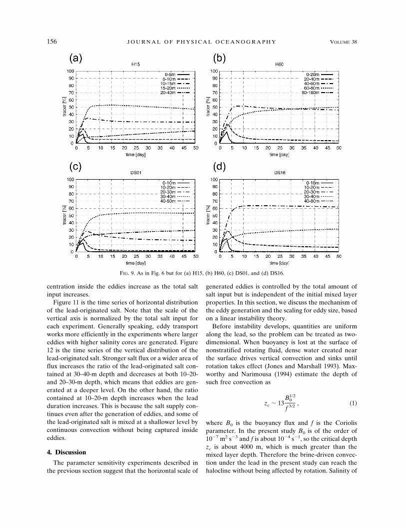
First we show the result of the experiments where themixed layer depth is set to 15 and 60 m (referred to asH15 and H60, respectively). The domain depth of themodel is 40 and 160 m, and the vertical resolution is1.25 and 5.0 m in H15 and H60, respectively. Figure 7shows the results at day 30. The lead-originated saltconcentration at the core of eddies is 0.10 psu in H15and as low as 0.03 psu in H60. Although there is a largedifference in the core concentration among these ex-periments, the horizontal size of the eddies is similar.However, the vertical scale of the eddies changes as themixed layer depth changes. Shorter eddies with highersalinity cores are generated in H15, and taller eddieswith lower salinity cores are generated in H60. (Notethat the vertical scale is different between Figs. 7b and7d.)

Next we show the results of the experiments afterchanging the strength of the halocline. In DS01 thedifference of salinity between the upper mixed layerand the dense water under the halocline, �S, is set to0.125 psu, which corresponds to a density difference of

FIG. 4. As in Fig. 2 (right column) but for (a) NORAND and (b) NOROT at day 10.


FIG

.5.T

ime

seri

esof

hori

zont

aldi

stri

buti

onof

the

lead

-ori

gina

ted

salt

inea

chre

gion

for

(a)

CT

RL

,(b)

NO

RA

ND

,and

(c)

NO

RO

T.

FIG

.6.T

ime

seri

esof

vert

ical

dist

ribu

tion

ofth

ele

ad-o

rigi

nate

dsa

ltfo

r(a

)C

TR

L,(

b)N

OR

AN

D,a

nd(c

)N

OR

OT

.


0.1 kg m�3; in DS16, �S � 2.0 psu (1.6 kg m�3). Theconcentration of the lead-originated salt and the scaleof eddies do not seem to be affected by the strength ofthe halocline, but the depth of the eddy core is different(Fig. 8). While convection reaches deeper than 40 mand the eddies are formed at the middle of the haloclinein DS01, the eddies are formed above the halocline andthe salt stays around 30-m depth in DS16 because pen-etrative convection is prevented by strong stratification.

The same analysis as in Fig. 5 shows a tendency simi-lar to CTRL for all of these four cases after changingthe halocline strength (figure not shown), so the lateralsalt transport by eddies does not seem to be affected bythe initial mixed layer depth or the strength of thehalocline. Contrary to the similarity in horizontal dis-

tribution, the vertical distribution of the lead-originatedsalt is different for the four cases (Fig. 9). While morethan 50% of the lead-originated salt is contained at20–30 m in DS01, more than 60% is contained at 30–40m in DS16. When the halocline is weak, the verticalconvection under the lead easily penetrates into thehalocline and eddies are formed at a deeper level. Oth-erwise, the convection is restricted by strong stratifica-tion and eddies are formed at a shallower level.

c. Sensitivity to the forcing parameters

We also investigate sensitivity to the surface salt fluxby changing the forcing parameters, that is, the appar-ent air temperature Ta, the width of the lead W, and theduration time of the lead ts; TA10 and TA40 are the

FIG. 7. As in Fig. 2 but for (a),(b) H15 and (c),(d) H60 at day 30.


same as CTRL, but Ta is �10° and �40°C, respectively.Low apparent air temperature leads to high ice growthrate, which results in a larger surface salt flux. In TA10,where the salt flux is weaker than CTRL, generatededdies are smaller and the concentration of the lead-originated salt at their core is smaller than in CTRL(Fig. 10a). In TA40, where the salt flux is stronger thanCTRL, the eddies are bigger and the core concentra-tion is greater than in CTRL (Fig. 10b). The depth ofthe peak of the salt concentration is also different be-cause the eddies sink to the depth where the density ofambient water matches the core density (figure notshown).

W02 and W04 are the same as CTRL, but W is 200and 400 m, respectively. The results (Figs. 10c,d) show

that a narrower lead induces smaller eddies withsmaller core concentration, and a wider lead inducesbigger eddies with higher core concentration. These re-sults are similar to the results of the experiments withchanging the apparent air temperature in terms of de-pendence on total salt input; that is, both lower airtemperature and a wider lead cause greater total saltinput, and both result in bigger eddies with higher coresalt concentration.

TS01 and TS10 are the same as CTRL, but ts is 1 and10 days, respectively. The longer duration time of thelead causes greater total salt input. Note that the totalsalt input and ts are not linearly related because thegrowth rate decreases as ice grows. Figures 10e,f alsoshow similar results; that is, the eddy scale and the con-

FIG. 8. As in Fig. 2 but for (a),(b) DS01 and (c),(d) DS16 at day 30.


centration inside the eddies increase as the total saltinput increases.

Figure 11 is the time series of horizontal distributionof the lead-originated salt. Note that the scale of thevertical axis is normalized by the total salt input foreach experiment. Generally speaking, eddy transportworks more efficiently in the experiments where largereddies with higher salinity cores are generated. Figure12 is the time series of the vertical distribution of thelead-originated salt. Stronger salt flux or a wider area offlux increases the ratio of the lead-originated salt con-tained at 30–40-m depth and decreases at both 10–20-and 20–30-m depth, which means that eddies are gen-erated at a deeper level. On the other hand, the ratiocontained at 10–20-m depth increases when the leadduration increases. This is because the salt supply con-tinues even after the generation of eddies, and some ofthe lead-originated salt is mixed at a shallower level bycontinuous convection without being captured insideeddies.

4. Discussion

The parameter sensitivity experiments described inthe previous section suggest that the horizontal scale of

generated eddies is controlled by the total amount ofsalt input but is independent of the initial mixed layerproperties. In this section, we discuss the mechanism ofthe eddy generation and the scaling for eddy size, basedon a linear instability theory.

Before instability develops, quantities are uniformalong the lead, so the problem can be treated as two-dimensional. When buoyancy is lost at the surface ofnonstratified rotating fluid, dense water created nearthe surface drives vertical convection and sinks untilrotation takes effect (Jones and Marshall 1993). Max-worthy and Narimousa (1994) estimate the depth ofsuch free convection as

zc � 13B0

1�2

f 3�2 , �1

where B0 is the buoyancy flux and f is the Coriolisparameter. In the present study B0 is of the order of10�7 m2 s�3 and f is about 10�4 s�1, so the critical depthzc is about 4000 m, which is much greater than themixed layer depth. Therefore the brine-driven convec-tion under the lead in the present study can reach thehalocline without being affected by rotation. Salinity of

FIG. 9. As in Fig. 6 but for (a) H15, (b) H60, (c) DS01, and (d) DS16.


FIG. 10. As in Fig. 2 (left column) but for (a) TA10, (b) TA40, (c) W02, (d) W04, (e) TS01, and (f) TS10 atday 30.


the water column under the lead is well homogenizedthroughout the mixed layer by such convection, and ahigh salinity water mass with sharp fronts is formedunder the lead. Such a localized dense water mass tendsto induce cellular overturning, but it is interrupted bygeostrophic adjustment in a few days. During geo-strophic adjustment, along-lead geostrophic jets de-velop at both fronts. Since the cellular overturning isconvergent at the surface and divergent at the base ofthe mixed layer, the directions of these geostrophic jets

are opposite between the surface and the base, and theysatisfy the thermal wind balance

��

�z�

1f

�b

�z, �2

where the buoyancy b is defined as

b � �� 0

�0g. �3

FIG. 11. As in Fig. 5 but for (a) TA10, (b) TA40, (c) W02, (d) W04, (e) TS01, and (f) TS10.


During geostrophic adjustment, the cellular over-turning circulation tilts the fronts, and the displacementof the fronts is scaled by the local internal deformationradius

Rd ��bH

f, �4

where �b is the buoyancy difference between insideand outside of the fronts (Dewar and Killworth 1990;

Send and Marshall 1995). Note that Rd is defined bylocal density anomaly induced by the freezing lead, notderived from the mean stratification.

The total buoyancy change of the dense water mass(the trapezoidal region in Fig. 13a) and the total buoy-ancy loss due to salt input at the surface should bebalanced:

WB0ts � �W � Rd H�b � �W � Rd Rd2 f 2. �5

FIG. 12. As in Fig. 6 but for (a) TA10, (b) TA40, (c) W02, (d) W04, (e) TS01, and (f) TS10.


Using a scaling argument, we can omit the lowest-orderterm. If Rd K W, (5) yields

Rd ��B0ts

f. �6

On the other hand, if Rd, k W, (5) yields

Rd � �WB0tsf 2 �1�3

. �7

When Rd � W, both (6) and (7) are satisfied except forthe factor of 2�1/2 in (6) and 2�1/3 in (7). In CTRL,B0 � 1.2 � 10�7 m2 s�3, ts � 3.0 � 105 s, and f � 1.4 �10�4 s�1, and (6) yields Rd � 1.2 � 103, but this value ofRd violates the assumption that Rd � W, so the formercase is not appropriate. On the other hand, (7) yieldsRd � 1.1 � 103 m, which is consistent with the assump-tion that Rd � W. All experiments in the present studysatisfy the condition Rd � W, so we adopt (7) as thescaling of the internal deformation radius Rd.

After a few days, baroclinic instability develops atboth fronts. Linear instability theory (Eady 1949; Ped-losky 1979) indicates that the wavelength of the fastestgrowing mode is

�c � 3.9Rd, �8

and its growth rate is

�c � 0.3f

Ri1�2 , �9

where Ri is the Richardson number

Ri �N2

��V��z 2 � f 2�b��z

��b��x 2 �10

and V is velocity of the along-lead jets. Since the hori-zontal scale of the front displacement is Rd � ��bH/fand the vertical scale is H, the Richardson number isscaled as

Ri � f 2�b��z

��b��x 2 � f 2�b�H

��b�Rd 2 � 1. �11

Therefore, the maximum growth rate is 0.3f, and thetime scale of the development of instability is estimatedas 1–2 days, in good agreement with the results of ourexperiments.

After closing of the lead, dense saline water forms adomelike structure (Fig. 13b). Based on the previousdiscussion, the distance between both fronts at the baseof the mixed layer is W � 2Rd, which is less than thewavelength of the fastest growing mode �c � 3.9Rd.Supposing that the amplitude of the perturbation in-creases up to its own wavelength, the meandering of thealong-lead jets induced by baroclinic instability devel-oped at both fronts divides the underlead dense waterregions into separated masses (Fig. 14). Since the densewater region has negative vorticity at the base, eachseparated dense water mass has anticyclonic circulationand is geostrophically balanced. The basal area of eachmass is scaled as

S � �c � �W � 2Rd � 10 � Rd2, �12

and it follows that the radius of eddies is scaled as

R ��S

�� 2Rd � 2�WB0ts

f 2 �1�3

. �13

Note that baroclinic instability generates pairs ofpositive and negative vorticity columns. The negativeones are generated in the dense water region inside the

FIG. 13. Schematic views of the structure of dense water mass and the direction ofalong-lead jets (a) before and (b) after closing of the lead.


fronts and form anticyclonic eddies with high salinitycores. Therefore, these anticyclonic eddies are in geo-strophic balance. On the other hand, positive vorticitycolumns are generated outside of the fronts, and thereis no mechanism for maintaining the positive vorticity.Consequently, only anticyclonic eddies survive.

Figure 15 is a plot of the radius of eddies generated inall experiments. The vertical axis is the radius, which isthe average distance between the core of eddies andtheir velocity maxima at 10 days after closing the lead.The horizontal axis is the scaled internal deformationradius as in (7). The radius looks approximately pro-portional to Rd, and least squares fitting yields

R � �1.81 � 0.03 � �WB0tsf 2 �1�3

. �14

This result is consistent with the scaling analysis (13),and it also agrees with the laboratory experiments ofBush and Woods (1999) in which the eddy radius isscaled as

R � �1.6 � 0.2 � �WB0tsf 2 �1�3

. �15

However, (14) does not agree with Smith et al. (2002) inwhich the eddy radius is scaled as

R �B0ts

f�16

or

R �B0

f 3�1�2

�17

when the condition ts � 1/f is used.

The reason for this disagreement is that the lead inSmith et al. (2002) is wider (720–5600 m), so (6) shouldbe adopted for scaling the deformation radius. In thepresent paper, the lead width is no greater than 800 mand all cases satisfy W � Rd, so (7) is adopted.

The term WB0ts in (14) stands for the product of thebuoyancy flux, the width where the flux is applied, andthe duration time of the flux, so it represents the totalbuoyancy loss per unit length of the lead. Since thenumber of generated eddies should be proportional tothe lead length and f is constant, (13) suggests that theradius of generated eddies is proportional to the cuberoot of the total buoyancy loss.

5. Summary and conclusions

We have performed numerical experiments to inves-tigate the effects of brine rejection under leads abovethe Arctic Ocean mixed layer. A three-dimensionalnonhydrostatic ocean model coupled with a thermody-namic sea ice model is used. The initial condition andthe surface forcing are set to a characteristic situation ofthe wintertime Arctic Ocean.

Brine-driven vertical convection caused by freezingof a lead forms density fronts in the mixed layer be-tween saline dense water under the lead and ambientrelatively freshwater. At such fronts, baroclinic insta-bility develops in a few days and separates the densewater mass into discrete anticyclonic eddies with a scaleof 3 to 5 km at the base of the mixed layer. Theseeddies, containing saline water, survive for over 50 daysand move horizontally in the mixed layer. Conse-quently, the salt that is supplied locally under the leadis transported by the eddies to a wider area.

The results of parameter sensitivity experiments sug-gest that the scale of the generated eddies is propor-tional to the cube root of the total buoyancy loss. This

FIG. 14. Schematic of eddy generation at the base of the mixedlayer under the lead.

FIG. 15. Plot of radius of eddies in all experiments except NORANDand NOROT. Error bar indicates resolution of the model.


conclusion agrees with scaling analysis using a linearinstability theory and the results of laboratory experi-ments (Bush and Woods 1999) but does not agree withthe results of the previous numerical experiments bySmith et al. (2002). The reason for this disagreement isthe difference in the choice of lead width W. While Wis less than the internal deformation radius in thepresent study, that used in Smith et al. (2002) is greater.

Our model result and previous studies (Smith et al.2002; Bush and Woods 2000) show that a line-shapedsalt flux under leads create baroclinic eddies. Subsur-face anticyclonic eddies with cold and high salinitycores have been observed in the Arctic Ocean (Manleyand Hunkins 1985; Muench et al. 2000), but their originis not yet clear. Those observed eddies are very similarto the eddies in our model in terms of their anticyclo-nicity, core T/S, and depth of kinetic energy peak. How-ever, the horizontal scale of these observed eddies istypically 10–20 km, which is much larger than the ed-dies in the present study. One possibility is that severalsmaller eddies generated under leads merge into alarger one. Note that those eddies are observed fromstations on moving ice floes, so small-scale eddies mightnot be detected. Another possible origin of the ob-served subsurface eddies is the baroclinic structure ofcoastal currents, discussed by Chao and Shaw (2003).

Distribution of the lead-originated salt is notable. Al-most all salt supplied under the lead is captured insidethe generated eddies, which exist just above the halo-cline. Therefore, the lead-originated salt settles only atthe base of the mixed layer and is not used to increasesalinity of the upper mixed layer. In many OGCMs, thesalt supplied as a result of freezing leads is uniformlydistributed over the mixed layer by convective adjust-ment or other boundary layer parameterizations, so itincreases the salinity uniformly over the mixed layer.This process decreases the density gap between fresh-water in the mixed layer and salty water beneath thehalocline, so the vertical structure of the halocline tendsto be broken. However, the result of the present studysuggests an opposite scenario; that is, the salt suppliedunder leads settles only at the base of the mixed layerand reinforces the salinity gap at the halocline. Param-eterizing these effects may improve representation ofthe Arctic Ocean mixed layer in OGCMs.

In the present study, we idealize the Arctic Oceanand omit some important factors, such as wind-drivendrift of the sea ice pack, thermodynamic growth of thicksea ice cover, and heat transport induced by upwellingof deeper warm water. In particular, drift of the sea icepack can significantly affect the vertical distribution oflead-originated salt because movement of the salt fluxprevents formation of sharp fronts and baroclinic ed-

dies. To develop a new parameterization of the ArcticOcean mixed layer, those factors should be investi-gated. We have actually performed moving ice packexperiments, and their results suggest that the lead-originated salt is distributed to shallower levels in themixed layer as the sea ice velocity increases. Those re-sults will be discussed elsewhere.

Acknowledgments. We acknowledge Prof. MasahiroEndoh and Dr. Yoshiki Komuro for helpful commentsand fruitful discussions. Thanks are extended to Dr.Akira Oka and Dr. Hiroaki Tatebe for helpful sugges-tions.

REFERENCES

Bush, J. W. M., and A. W. Woods, 1999: Vortex generation by lineplumes in a rotating stratified fluid. J. Fluid Mech., 388, 289–313.

——, and ——, 2000: An investigation of the link between lead-induced thermohaline convection and arctic eddies. Geophys.Res. Lett., 27, 1179–1182.

Cavalieri, D. J., and S. Martin, 1994: The contribution of Alaskan,Siberian, and Canadian coastal polynyas to the cold haloclinelayer of the Arctic Ocean. J. Geophys. Res., 99 (C9), 18 343–18 362.

Chao, S. Y., and P. T. Shaw, 2003: A numerical study of densewater outflows and halocline anticyclones in an arctic baro-clinic slope current. J. Geophys. Res., 108, 3226, doi:10.1029/2002JC001473.

Dewar, W. K., and P. D. Killworth, 1990: On the cylinder collapseproblem, mixing, and the merger of isolated eddies. J. Phys.Oceanogr., 20, 1563–1575.

Eady, E. T., 1949: Long waves and cyclone waves. Tellus, 1, 33–52.Griffies, S. M., and R. W. Hallberg, 2000: Biharmonic friction with

a Smagorinsky-like viscosity for use in large-scale eddy-per-mitting ocean models. Mon. Wea. Rev., 128, 2935–2946.

Haney, R. L., 1971: Surface thermal boundary condition for oceancirculation models. J. Phys. Oceanogr., 1, 241–248.

Jones, H., and J. Marshall, 1993: Convection with rotation in aneutral ocean: A study of open-ocean deep convection. J.Phys. Oceanogr., 23, 1009–1039.

Kantha, L. H., 1995: A numerical model of Arctic leads. J. Geo-phys. Res., 100 (C3), 4653–4672.

Kozo, T. L., 1983: Initial model results for arctic mixed layer cir-culation under a refreezing lead. J. Geophys. Res., 88 (C5),2926–2934.

Leonard, B. P., 1979: A stable and accurate convective modelingprocedure based on quadratic upstream interpolation. Com-put. Methods Appl. Mech. Eng., 19, 59–98.

——, 1991: The ultimate conservative difference scheme appliedto unsteady one-dimensional advection. Comput. MethodsAppl. Mech. Eng., 88, 17–74.

——, A. P. Lock, and M. K. MacVean, 1996: Conservative explicitunrestricted-time-step multidimensional constancy-pre-serving advection schemes. Mon. Wea. Rev., 124, 2588–2606.

Manley, T. O., and K. Hunkins, 1985: Mesoscale eddies of theArctic Ocean. J. Geophys. Res., 90, 4911–4930.

Marshall, J., A. Adcroft, C. Hill, L. Perelman, and C. Heisey,1997a: A finite-volume, incompressible Navier–Stokes model


for studies of the ocean on parallel computers. J. Geophys.Res., 102 (C3), 5753–5766.

——, C. Hill, L. Perelman, and A. Adcroft, 1997b: Hydrostatic,quasi-hydrostatic, and nonhydrostatic ocean modeling. J.Geophys. Res., 102 (C3), 5733–5752.

Maxworthy, T., and S. Narimousa, 1994: Unsteady, turbulent con-vection into a homogeneous, rotating fluid, with oceano-graphic applications. J. Phys. Oceanogr., 24, 865–887.

Maykut, G. A., 1982: Large-scale heat exchange and ice produc-tion in the central Arctic. J. Geophys. Res., 87, 7971–7984.

Muench, R. D., J. T. Gunn, T. E. Whitledge, P. Schlosser, and W.Smethie Jr., 2000: An Arctic Ocean cold core eddy. J. Geo-phys. Res., 105 (C10), 23 997–24 006.

Pedlosky, J., 1979: Geophysical Fluid Dynamics. Springer-Verlag,710 pp.

Rudels, B., L. G. Anderson, and E. P. Jones, 1996: Formation andevolution of the surface mixed layer and halocline of theArctic Ocean. J. Geophys. Res., 101 (C4), 8807–8822.

Semtner, A. J., 1976: Model for the thermodynamic growth of seaice in numerical investigations of climate. J. Phys. Oceanogr.,6, 379–389.

Send, U., and J. Marshall, 1995: Integral effects of deep convec-tion. J. Phys. Oceanogr., 25, 855–872.

Skyllingstad, E. D., and D. W. Denbo, 2001: Turbulence beneathsea ice and leads: A coupled sea ice/large-eddy simulationstudy. J. Geophys. Res., 106 (C2), 2477–2498.

Smith, D. C., and J. H. Morison, 1993: A numerical study of halineconvection beneath leads in sea ice. J. Geophys. Res., 98 (C6),10 069–10 084.

——, and ——, 1998: Nonhydrostatic haline convection underleads in sea ice. J. Geophys. Res., 103 (C2), 3233–3248.

——, J. W. Lavelle, and H. J. S. Fernando, 2002: Arctic Oceanmixed-layer eddy generation under leads in sea ice. J. Geo-phys. Res., 107, 3013, doi:10.1029/2001JC000822.

Smith, S. D., R. D. Muench, and C. H. Pease, 1990: Polynyas andleads: An overview of physical processes and environment. J.Geophys. Res., 95 (C6), 9461–9479.

Steiner, N., and Coauthors, 2004: Comparing modeled stream-function, heat and freshwater content in the Arctic Ocean.Ocean Modell., 6, 265–284.


brine-driven eddies under sea ice leads and their … eddies under sea ice leads and their impact on...

Documents