broadlband analysis and synthesis of antennas and scattererssaito/data/sonar/baum-iproc.pdf ·...

1598 PROCEEDINGS OF THE IEEE, VOL. 64, NO. 11, NOVEMBER 1976

Emerging Technology for Transient and BroadlBand Analysis and Synthesis of

Antennas and Scatterers

CARL E. B A m , MEMBER, IEEE

Invited Paper

A&muct-Duetosomerppliedprob&msofreantint8redtsigWant efforthmbeendevotedtodew4opingtbefecbn~ofthetrmdent and b d - b m d electranqnetic ~lpon& of v d o w object8 such as m C e a n r r d ~ m ~ a ~ n t r t b e p ~ ~ a t - r = s u c h trmdenthldk ~ p g e r ~ l l l e v a r i o M t y p e r o f r p p r a r h e s which haw been wed for lmdeatrnding such trm&nt/broad-baud ptopsrtiw. WhIteiuitidlyvdowrpprode8aidinrndylofmcb &4ds,insomecrrerotherpropertkofthepprode8leadtomore ~ ~ n s u l g ~ c h ~ s y n ~ o f ~ n t l b r o r d - b d p r o p e r t i e a

R 1. INTRODUCTTON

ECENT YEARS have shown significant attention being given to the development of basic and applied understanding of that part of electromagnetics which is often

referred to by that generic term of "transient." In a general sense transient may refer to any nonmonochromatic (or non- CW) electromagnetic problem. However, such a definition is perhaps too broad to be useful. Sometimes nonmonochromatic problems are analyzed or solved experimentally using single frequency concepts applied to some narrow band of frequencies; such cases are excluded from consideration in this paper. For this paper transient and broad band will be used somewhat interchangeably because of the close relation of the time and frequency (broad-band) domains and the use of concepts which give information about both domains simultaneously.

A. Background In the early investigations of basic electromagnetic phenom-

ena (say through most of the Nineteenth Century) there was no discussion of transient versus continuous wave (CW) electromagnetics. Electric and magnetic phenomena were understood in a static sense and the time derivative terms were next introduced. All the experiments were static or transient in nature. It was only when light was later shown to be an electromagnetic phenomenon that CW concepts (such as wavelength) were introduced. Even then the experiments below the microwave region were of a transient nature, including damped sinusoids [SI. Even wire telegraphy was transient and wire telephony involved broad-band distortionless (Le., transient) transmission [ 31.

With the development of wireless telegraphy and radio the emphasis shifted to CW electromagnetic concepts. Now there was some carrier or center frequency on which information was modulated in the form of some narrow bandwidth around

Manuscript received J a n u a r y 13,1976. revised June 28,1976. The author is with the Air Force Weapons Laboratory, Kirtlrnd

AFB, NM 87117.

the carrier frequency. The introduction of radar continued this trend toward CW electromagnetic development.

In recent years, some new problems have appeared on the scene to shift some of the emphasis back toward transient considerations. One class of problems involves protection of electronic equipment from the effects of strong transient fields. This includes the nuclear electromagnetic pulse ( E m ) and lightning in particular. As an outgrowth of the efforts in these areas some of the new understanding is being applied in some areas of electromagnetic inverse scattering, in particular remote sensing and radar scatterer discrimination. These interests have extended to the basic phenomenology of the transient electromagnetic field generation, to sensors (special antennas) for measuring the transient fields, to simulators (special antennas) [ 2 6 ] for producing desired temporal and spatial electromagnetic field distributions, and to the interaction of such field distributions with very complicated scatterers. With respect to EMP in particular the technology is quite extensive and the reader is referred to an upcoming special issue of the IEEE Transactions on Antennas and Propagation on the subject.

It should be noted that even some CW problems are showing transient aspects as their bandwidths (say for communication or radar) are increased. Dispersion can be important when short RF bursts, in particular, are used.

In trying to understand the transient electromagnetic problem one attempts to look at the subject in new ways so as to exhibit important features of the problem that may not be so apparent from a CW point of view. In this quest it is useful to go back to the sources to see the insights and clues given by some of the important early investigators [ 1 I -[ 3) . At a minimum such works stimulate one's intellect to some unac- customed ways of thinking.

A recent book [ 131 addresses some of the important topics in transient electromagnetics in some detail. The reader is referred to this work as a general reference for the topic under discussion here.

B. Conventions In this paper when time harmonic waves are considered the

time dependence eiwr is used. For more general purposes the Laplace transform is defined in a two-sided sense as

&) = F(t)e-" d t

F ( t ) = - I F(s)eS' ds

u o+i-

27n' a , - i m

BAUM: ANALYSIS AND SYNTHESIS OF ANTENNAS AND SCATTERERS 1599

with the contour CO from 52, - io0 to no + io0 to the right of all singularities in the s plane. Here F ( t ) may be a scalar, vector, dyadic, etc., function of time. This Laplace transform de- fines the complex frequency

s = f i + i w . (1.2)

The time harmonic form of the solution is obtained by setting fi = 0. A tilde - over a quantity indicates the Laplace transform; this notation then is used for the time harmonic form.

The symmetric product (similar to the inner product) is indicated by

(&, r‘) ; b(r’)> = 5 z ( r , r‘) * b ( r ‘ ) K ) (1.3) S or V

where integration is over some surface or volume which may be specified or left in a general form. The comma separates quantities with a common variable of integration. The dot (or other symbol) directly above the separating comma indicates the multiplication sense as a dot product (or other type of product). This symmetric product can involve two, three, etc., integrations by use of additional commas and the inte- grands can be scalar, vector, or dyadic quantities. The inte- grands may also be functions of complex frequency s or time t and integration may or may not be included over such variables as desired. If two or more ranges of integration are used then subscripts can be placed on ( ,> and/or certain integrations indicated explicitly.

C. Basic Equations

Maxwell’s equations with equations of continuity as The starting point of transient electromagnetics is of course

a at

a a t

V X E(r, t ) = - - B(r, t ) 7 J, ( I , t )

V X H(r, t ) = - D(r, t ) + J(r, t )

a a at at a a at at

V * J(r, t ) = - - V * D(r, t ) = - - p(r, t )

V . J , ( ~ , t ) = - - V . B ( r , r ) = - - p , ( r , r ) (1.4)

where magnetic currents and charges have been included for generality. The constitutive relations (including Ohm’s Law) are ... - ...

D(r, s) = z(r, s) * E(r, s), zr, s) = z(r, s) g(r , s)

B(r, s) =&, 8 ) - H(r, s), J,,, (r, s) = z, (r, s) - H(r, s)

... ... .., ... .,v .., ...

(1.5)

where the current densities in this case do not include sources. In time domain these relations are

D(r, t ) = 2 ( I , t ) E(r, t) , J(r, t ) = 5 ( I , t ) f E(r, t )

B(r, t ) = &r, t ) t H(r, t) , J , (r, t ) = Z(r , t ) t H(r, t )

(1.6)

where * indicates convolution over time. More general forms of the constitutive relations are possible including nonlinearities and more general linear relations among the field components. For most of this paper the sirnple free space (or equivalently

uniform isotropic medium) relationships are chosen as

D(r, t ) = € O W , t ) , B(r, t ) = 110H(r, t ) (1.7)

with + ... ... + u (r, s) = 2, (r, s) = 0

except perhaps in some localized region of interest. Define

- 1 c=- G speed of light

20 E wave impedance

y=- propagation constant

7 = c t time in distance units. (1.8)

S

C

In solving Maxwell’s equations it is convenient to introduce the Green’s functions. The free-space Green’s functions satisfy [ I l l

[ vz - 7 2 1 G&, r’; s) = -6(r - r‘)

[ v x v x + 7 2 1 Zo(r , rr ; s )= ia (r -rr ) (1.9) ...

where 7 is the identity dyadic (1 with a subscript being a unit vector) and 6(r - r ’ ) is the threedimensional delta function. The radiation conditions (with Re[$] 2 0) are

... lim r [ V + y l t l X&(r ,r ’ ; s )=O.

+ (1 .lo)

? +

Defining

{ E y l r - r ‘ I , R = r - r ’ , R = I R I (1.11)

explicit representations of the Green’s functions are

1 --* + - 6(r - r‘)l 3Y2

(1.12)

where strictly speaking r # I ‘ but for singular integrals the principal value integral is implied and for distributions such as 6(r - r’) their usual rules apply so as to give the proper behavior when integrated over current densities [ 391 , [ 8 1 ] . For use with surfaces (instead of volumes) slightly different conditions apply, in particular at r = r’.

1600 PROCEEDINGS OF THE IEEE, NOVEMBER 1976

Here all polarizability and conductivity effects are included as part of the two current densities.

D. Integral Equations For general shapes and impedance loading distributions on

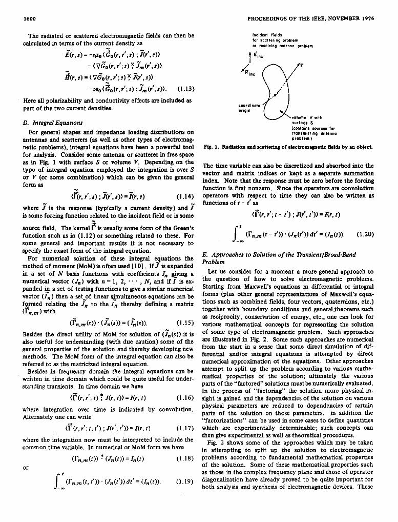
antennas and scatterers (as well as other types of electromagnetic problems), integrd equations have been a powerful tool for analysis. Consider some antenna or scatterer in free space as in Fig. 1 with surface S or volume V. Depending on the type of integral equation employed the integration is over S or Y (or some combination) which can be given the general form as -

( f i r , r‘; s) ; Zr‘, 8 ) ) = &, s) (1.14)

where 7 is the response (typically a current density) and is some forcing function related to the incident field or is some

source field. The kernel I-‘ is usually some form of the Green’s function such as in (1.12) or something related to these. For some general and important results it is not necessary to specify the exact form of the integral equation.

For numerical solution of these integral equations the method of moment (MOM) is often used [ 101. If f is expanded in a set of N basis functions with coefficients J, @ving a numerical vector ( J , ) with n = 1, 2, - - , N, and if I is expanded it~ a set of testing functions to give a similar numerical vector ( I , ) then a set-of linear s@ultaneous equations can be fgrmed relating the J, to the I , thereby defining a matrix

N +

V n , m with

<i;,,m(s>> * (%(SI> = (c(s)). (1.15) Besides the direct utility of MOM for solution of (Tn(s)) it is also useful for understanding (with due caution) some of the general properties of the solution and thereby developing new methods. The MOM form of the integral equation can also be referred to as the matricized integral equation.

Besides in frequency domain the integral equations can be written in time domain which could be quite useful for understanding transients. In time domain we have

+(r, r f ; ’r) t ~ ( r , t ) ) = ~ ( r , r) (1.16)

where integration over time is indicated by convolution. Alternately one can write

--+ (r (r, r‘; r, t’) ; ~ ( r ’ , t ’ ) ) = z(r, t ) (1.17)

for rcatterinq problem incident fields

or receiving antenno problem

coordinate wigin

volume V with surface S (contains sources for transmitting antenna problem)

Fig. 1. Radiation and scattering of ekctromagnetic field8 by an object.

The time variable can also be discretized and absorbed into the vector and matrix indices or kept as a separate summation index. Note that the response must be zero before the forcing function is f i t nonzero. Since the operators are convolution operators with respect to time they can also be written as functions of t - t’ as

<i$r, r’; r - t‘) ; ~ ( r ‘ , t’)) = ~ ( r , t )

L (r,,m(t - t‘)) - (Jn(t‘)) dt‘ = (I,(r)). (1.20)

E. Approaches to Solution of the lYansient/Brwd-Band Problem

Let us consider for a moment a more general approach to the question of how to solve electromagnetic problems. Starting from Maxwell’s equations in differential or integral forms (plus other general representations of Maxwell’s equations such as combined fields, four vectors, quaternions, etc.) together with boundary conditions and general,theorems such as reciprocity, conservation of energy, etc., one can look for various mathematical concepts for representing the solution of some type of electromagnetic problem. Such approaches are illustrated in Fig. 2. Some such approaches are numerical from the start in a sense that some direct simulation of differential and/or integral equations is attempted by direct numerical approximation of the equations. Other approaches attempt to split up the problem according to various mathematical properties of the solution; ultimately the various parts of the “factored” solutions must be numerically evaluated. In the process of “factoring” the solution more physical insight is gained and the dependencies of the solution on various physical parameters are reduced to dependencies of certain parts of the solution on those parameters. In addition the “factorizations” can be used in some cases to define quantities which are experimentally determinable; such concepts can then give experimental as well as theoretical procedures.

Fig. 2 shows some of the approaches which may be taken in attempting to split up the solution to electromagnetic problems according to fundamental mathematical properties of the solution. Some of these mathematical properties such as those in the complex frequency plane and those of operator diagonalization have already proved to be quite important for both analysis and synthesis of electromagnetic devices. These


_ _ _ _ _ _ - - - - - - Morwell's Equotions

integrol ond differential forms various mothemoticol representotions

boundory conditions general relations

integral eqmtions

I I I I I numericol solution of

in time domain in frequency domain differential equations differential equations numerical solution of

I a- I

numerica I I anolyticbl fram the I from t h

star t I star t

Fig. 2. Approache8 to solution of Maxwell's equationa.

onalytic s plane oppooch

high frequency ar early time asymptotics

1 IM; 1 integral operator madol approach

P eigenmodcs

intermediate and low frequencies modes or intermediate and Iote time

chorocteristic

S E M

low frequency or late time asymptotics

LFM

Fig. 3. Division of some approaches into methods.

approaches can be further subdivided into methods as illustrated in Fig. 3; some of these methods are later considered in some detail. The future of transientbroad-band electromagnetics may well consist in the investigation of new approaches and the resulting methods under such approaches, as well as the detailed techniques for actual calculations under each method. This paper reviews approaches which have been investigated to an extensive degree to date. Some of the less investigated ones such as differential geometry for transient lens design [ 171, [28], topological properties of complicated scatterers [70], [89], and group theoretic properties (symmetries) [ 411, all appear to have some significant potential for future development.

11. NUMERICAL INVERSE FOURIER TRANSFORM OF FREQUENCY -DOMAIN SOLUTIONS

Except for special transient problems leading to closed form solutions, transient scattering and antenna problems for more

general structures were f i t treated by numerical inverse Fourier transforms of frequencydomain solutions. While this type of solution sheds little physical insight into the characteristics of the transient response it was still used to obtain some of the early numerical calculations of transient responses. It should be noted that inspection of the resulting waveforms as well as experimental transient waveforms played a role in developing methods which do exhibit greater physical insight into the scattering process.

It is not our intent to dwell here on the techniques of numerical Fourier analysis. The common algorithm for such numerical transforms is often referred to as the fast Fourier transform (FFT) [ 12, ch. 71 which has been applied to many fields. An important feature of the FFT is that it uses uniformly spaced samples of frequency and time to take advantage of the periodicity of the function e ' iwr with period of 2n for ut. For some problems such uniform spacing may not be optimum because of the relative importance of various por-


tions of a frequency spectrum in constructing a transient waveform. Some success for broad-band transients has been obtained using frequency samples spaced Aw where Aw/o is approximately constant [ 7 1 ] . Special- difficulties are encoun- tered when the function to be transformed has singularities on or near the integration contour (the iw~axis in the s plane); these can be handled but special attention is required.

In its commonly applied form numerical Fourier transforms have been used in conjunction with MOM numerical solutions in frequency domain. Assuming that the scattering or antenna problem as in Fig. 1 is cast in MOM form (1.1 5 ) we have the formal solution in complex frequency domain as

(G(s>> = (Fn,m(S))-l * (Tn(s>> (2.1) which is specialized to s = iw as

( 7 n ( i ~ ) ) = (Fn,m ( i ~ ) ) - l ( ? n ( i ~ ) ) . (2.2)

The inverse Laplace transform (1.1) is then obtained as'

where the integral over w is o b t e e d numericallx. Note that 3 there are any singularities of (I'n,m(s))-l or (In($)) on the io axis of the s plane (or to the right of the iw axis) then the integration over w must be suitably modified.

A closely related procedure which could be used is to first compute

1 W

(In 0)) = I, (Fn (iw))eiw' dw

Then use the convolution theorem

(Jn(t)) = ( A n , m ( t ) ) ' ( I n ( t ) ) - (2.5)

In the commonly applied form (2.3) the numerical inverse Fourier transform has some significant limitations. Specifically the solution ( J n ( t ) ) must be largely recomputed for many changes in the input parameters of the probles. Such changes can be introduced in the forcing function (In(iw)) via direction of incidence, waveform or other zharacteristics of the incident or source field. The matrix (rn,m(iw)) (operator) accounts for changes in object shape and impedance loading. The solution contains the effects of these changes in a complicated manner and it is difficult to uniquely identify particular aspects of the solution with specific input parameters.

The convolution extension of the numerical inverse Fourier transform (2 .5 ) has the added advantage of separating the effects on the solution due to the operator from those due to the forcing function, at least to some degree. Note that (a4n.m ( t ) ) is an N X N matrix with each element being a function of

time and numerically characterized by say M time samples. This allows the object shape andimpedance characteristics to enter the computation and be stored while the forcing function is changed, but imposes a significant storage requirement intheformofaniVXNXMarray.

An advantage of the numerical inverse Fourier transform approach is the better understanding of the convergence criteria for numerical Fourier integrals than for some of the expansions to be discussed later. This technique can then be used to compare against the solution of the same problem obtained by other means to check validity, say in a few cases, as required. For problems limited to only one set of input parameters and say a single frequency or a single forcing transient waveform this approach is still quite efficient in comparison to other methods of solving the matricized integral equation (MOM) in frequency or time domain.

Numerical inverse Fourier transform solutions or those using other expansions have a common limitation if they use MOM as their numerical basis. Specifically MOM imposes a high-frequency (or fast-time) limitation associated with the accuracy of the MOM approximation. The limitation is associated with the ratio of wavelength to zone size or similar characteristic dimension in the basis and testing functions. One can increase the number of zones (decrease zone size) to go to higher frequencies to obtain more accurate early time response, but one is limited in this regard by practical compu- tational capability.

III. ANALYTIC s PLANE APPROACH

One approach to the solution of transient/broad-band problems centers around the properties of the solution in the s(= 52 + iw) or complex frequency plane. Using concepts from complex variables the sources, operators, and solutions may be expanded in various kinds of series to give greater physical insight into the behavior of the response for certain time and/or frequency regimes, to simplify the parametric representation (display) of the response characteristics, and to reduce the amount of numerical computation required for obtaining sets of solutions.

There are several types of series one can construct in the s plane. Power (Taylor) series can be defied about a point of analyticity in the s plane. More generally negative integer powers (poles) can also be included in such series (Laurent) if the center of the expansion is at a pole singularity. This type of series is particularly useful when centered at s = 0; this type of series expansion constitutes the low-frequency method (LFM) with powers of s becoming derivatives in time domain. Singularity series (sums of poles, branch integrals, essential singularities, and entire functions) can be defied based on the s plane singularities which is useful for expressing the transient/ broad-band response for cases that important wavelengths are of the order of the physical dimensions of interest or larger; this is the singularity expansion method (SEM) which has received much recent attention. Asymptotic series for s + m form the basis of the high-frequency method (HFM); such asymptotic series give series of time domain functions applic- able to the early-time response.

While the s plane approach starts from the problem formula- tion in frequency domain (in general complex), the resulting series are expressible in both frequency and time domain forms via the term-by-term application of the Laplace transform (including its inverse). Both frequency- and timedomain forms are thus implied in the methods discussed.


A . Low-Frequency Method Little has been done in the way of developing a systematic

transient representation based on low-frequency properties, but such a representation is at least conceptualiy rather straightforward. For finite size objects in free space the frequencydomain representation has been considered by Ray- leigh [771 and more recently by Stevenson [ 801, Kleinman [ 8 4 ] , and Kleinman and Senior [ 8 5 ] . This results in the response being represented by a power series in the complex frequency with a radius of convergence governed by the locations of the singularities of the response in the complex frequency plane.

In this paper, let us consider the leading terms in the low- frequency response for finite size objects in free space. Pro- vided the observation position is sufficiently far from the object (say several times the maximum dimension or greater), and provided the radian wavelength is large compared to the object then the dipole moments of the object govern the scattered fields (or total fields in the case of a transmitting antenna). Let us write the induced electric and magnetic dipole moments for a scatterer approximated as located at r' as

~ ( t ' , s ) = ~ ( ~ ) ~ ~ ~ ~ ~ ( ~ ' , ~ ) = - M ( s ) . ~ ~ ~ ( r ' , s ) (3.1)

where ?(s) and 30) are the electric and magnetic polarizability dyads, respectively, with dimensions of cubic meter. These are allowed to be functions of frequency in the general case to account for impedance loading of the object. For perfectly conducting objects and within the aforementioned frequency restrictions the polarizability dyads can be considered as constants.

The radiated or scattered fields associated with such dipole moments are computed as [ 81 , [ 231

... 1 1

cco .., ..,

bronch branch

X I I oole I I

I I c a

branch contour Co: R e [s) = O0

cut point

Fig. 4. s plane with some singularities and the inversion contour C,.

Hence for waveforms with dominantly only low-frequency components so as to require only the dipole moments for dis- tant scattered fields, the scattered waveform can be thought of as the sum of 3 simple waveforms found as proportional to the original waveform and its first and second time derivatives with a time shift (retarded time). If the polarizability dyads are also frequency independent of the low frequencies of interest then the scattered fields are related to the incident fields in this same manner (incident waveform plus its f i t and second time derivatives).

This result then is readily physically interpretable in time domain and provides a simple way to view low-frequency- dominated transient scattering for finite-size objects in free space if the observer is not too close to the scatterer. These results can be extended to more complicated higher order terms in the multipole expansion if desired. Note that (3 .3) can also have the operators in convolution form as discussed in Section I-D; however, the time derivative form provides an al- ternate form as well as simple physical interpretation.

B. Singularity Expansion Method

where the Green's functions are discussed in Section I-C. In going to time domain we can write

+ + R - ' [ - I + 1 R 1 R ] -

sponse is a real-valued time function. Consider a contour CO

Moving up into the resonance region we are led to the SEM concerning which extensive work has already been done. This author has written a more extensive review of this topic including many more examples in a recent book [ 13, ch. 31 ; this also contains a more detailed development and more references.

The general SEM formalism began from experimental obser- vations concerning the transient electromagnetic response of complicated scatterers such as missiles and aircraft [ 4 5 ] . It was observed that damped sinusoids were dominant features of typical transient responses. Such damped sinusoids corresponded to pole pairs in the complex frequency (or s) plane. Poles were one type of singularity in the s plane and this led to the concept of using all the s plane singularities to form a description of the transient and frequencydomain responses. It was also noted that the poles corresponded to the natural frequencies which had been discussed in some of the older literature as referred to in some texts [ 4 ] .

The basic concept then involves taking the Laplace transformed response and finding all the s plane singularities such as poles, branch points (and associated cuts), essential singularities, and singularities at infinity (or the entire function) as the description of the response. As illustrated in Fig. 4 we have a set of singularities in the left half of the s plane (for stability of a passive antenna or scatterer). The singularities are located symmetrically with respect to the Re [ s ] axis since the re-


to invert the Laplace transform back into time domain. De- form this contour into the left-half plane to obtain the contributions associated with each singularity and thereby define the terms in a singularity series (including any singularity at infinity).

While in principle several types of singularity terms may appear in the response, pole terms have proven to be most important for certain types of antennas or scatterers. In particular it can be shown that the inpulse response of a finite size object in free space has only pole singularities in the finite s plane provided the object is perfectly conducting or is made of suitably simple media [451, [461, [481. A simple way of observing this property is to consider the inverse of the ma- t+ in the moment method (1.1 5) . Since the elements of (r,, (s)) are singe valued malytic functions of s with at most poles (since the r,,m are typically the Green's function for two points on the object with R finite) then the determinant has at most poles in the finite plane and the inverse matrix has at most poles in the finite plane.

If a is an index set for the natural frequencies sq let us write the response (current) of the object (Laplace transformed) to a delta function excitation as [451, [461, [511

q p ( r , s) = Ga(1 f , s)@ (rXs - S p Q CY

+ entire function contributions

mu = a positive integer (3.4)

where the equations for the factors in the pole terms are given below. The pole order mu may be greater than 1 in some special cases but we will concentrate on mu = 1. The direction of incidence (if required) is l1 and the polarization is indicated by the index p . The superscripts identify the quantity (current, charge, etc.) under consideration; often this superscript will be suppressed in the case of current.

From the integral equation for the delta function response I

I

( r q ( r ) ; r (r, r'; s q ) ) = o (3.6) i

which in MOM form reduces to

@ , m (sa 1) . ( ~ n )a = (0,

tee,), * ( i ;n,m(su)) = (0,) (3.7)

with a resulting equation for the natural frequencies as

det <<fn,m(sq))) = 0. (3.8)

For subsequent discussion only the operator form is normally listed; as above the matrix form is quite similar.

Expand terms in the integral equation near s = s, as

r(f, r' ;s) = - s,)l r lq(r, 7 OD -b

1=0

S'SQ

C(r, 3) = G U ( l 1 , sa) ru(r)(s - sa)-'

+ vector function analytic near so. (3.9)

Substituting these expansions into the integral equation (3.5) and collecting according to powers of s - sq we have for the (s - sU)-l term

-t

( r oq(r, r f ) ; GJI 1 , sa) va(r)) = o (3.10)

consistent with equations (3.7). The (s - sq)O term gives

(r oq(r, rf) ; vector function ofr') +

-b

+ ( r ~ ~ ( r , r ' ) ~ ~ q ( l l , ~ q ) ~ u ( ~ ' ) ) = ~ ~ ~ ( ~ ) . (3.11)

Left operate by pq(r ) to remove the fmt term (via (3.6)) and rearrange the results to give

(r&) ; z o p

( ra ( r ) ; l q k r') ; vq(r')) G u ~ l l r ~ u ) =

= coupling coefficient at sq. (3.12)

Having developed the equations for the natural frequencies and the residues of the corresponding poles one should note that the coupling coefficients ijq(ll , s) are only constrained by these equations at s = sq. For s # so various functional dependencies on s are possible. Two classes of coupling coefficients have been used successfully. Class 1 is the simpler and isgivenby [451, [511

(cqW ;Zoq(r)) Gq(ll ,s)=exp [(x, -s ) t ' ]

; r l q ( ~ ~ r ' ) ; vq(rf)) +

(3.13)

while class 2 is

iia(11,s)= + . (3.14)

Class 1 corresponds to a direct pole expansion of the response with frequency independent "residues" for a turn on time t ' (a simple shift of zero time); these coupling coefficients can be considered as constants (other than the possible simple shift). Class 2 corresponds to the direct pole expansion of the inverse operator (a dyadic) as

(r&) ;&,s))

( ra ( r ) ; 1& r') ; *&'N

+ entire function contributions (3.15)

and then operation onto the forcing function; note the dyadic residues in (3.1 5) . Observe that at s = sq both class 1 and class 2 coupling coefficients reduce to the same thing (3.12); they differ by an entire function which can then be included in the additional entire function contributions where required. Both forms of coupling coefficients have been used with good results [321, [401,[451, [481, [491, [521-[561.

BAUM: ANALYSIS AND SYNTHESIS OF ANTENNAS AND SCATTERERS 160s

In the case of the perfectly conducting sphere it has been shown that, with t' chosen as the time a plane wave first reaches the surface, the class 1 coupling coefficients give the exact response with no additional entire function [45 1. For this same problem it has also been shown that the class 2 coupling coefficients also require the inclusion of no additional entire function [491. The class 1 form is much simpler and requires much less information for specifying it over the range of variation of the incident wave parameters; except for a de- lay it is not frequency dependent. Even if an additional entire function is required in some cases, it may be useful to keep the entire function as a separate term. On the other hand, the class 2 form makes each pole term rise smoothly for early times, perhaps giving better convergence at early times. Even for class 2, however, it is not yet established whether an additional entire function is needed in the general case.

It would appear that the question of the entire function and its relation to the classes of coupling coefficients (including 1 and 2 and others that might be proposed [ 5 1 I ) is an important topic for future research. While all coupling coefficient classes must be consistent with (3.1 2) (for firstader poles) one can add an entire function with a zero at su to obtain another form satisfying (3.12). This corresponds to adding an entire function to the pole term 5 ~ 1 l , ,>viJ) (r)(s - su)-'.

One promising approach to pinning down the entire function contribution is based on the imposition of causality requirements, or more stringently, passivity requirements on the object response. Note that the individual pole terms need not be causal, but the total solution must be causal. More signifi- cantly certain types of responses are positive real (PR) functions in the usual circuit theory sense. Such cases correspond to the impedance or admittance at the gap of an antenna, as well as eigenimpedances (4.20) and eigenadmittances (4.21). The PR property constrains the solution in the right-half s plant including the asymptotic behavior as s + 00 and s + 0. Using these and other considerations for high and low frequencies one can restrict the class of allowable entire functions in the total response to some degree [ 901 , [ 9 1 ] . In effect this corresponds to imposing some necessary conditions, but does not necessarily give sufficient conditions.

Another promising approach involves the expansion of the response in eigenmodes discussed in Section IV, followed by the singularity expansion of each term in the resulting series.

Having found the delta function response of the object the current density response can be found from

&,s) = Q r , s ) p=2,3

jp(r , s) = Eo $&(s) (r, s) (3.16)

where Eo is a convenient source electric-field amplitude, $ is a scaling constant used in d e f i i g the delta function response. Where needed p = 2, 3 corresponds to polarizations_l~ and 13 which with l1 are mutually orthogonal. Here f p ( s ) is the Laplace transform of the sour_ce waveform.

Noting that the waveform f p ( s ) itself has a singularity expansion one can separate the effects of the object and waveform singularities in the response. The normalized response can be written as

Vf' (r , s) = &(s) C$J)(r, s) %

= ?'':)(r, s) + vP, - ( I ) ( r , s) (3.17)

where the object and waveform parts, respectively, are

= (singularities of&)) t?ja(r, s) J at fp s i n g u l a r i t i e s

(3.18)

with e n 9 function contributions neglected. The introduction of fp(su) in the object part of the response shows how the incident waveform scales the residues of the object poles (natural frequencies). For simple incident waveforms such as step functions the waveform part of the response becomes the low- frequency (s + 0 or static) response times a pole at s = 0 (step in time domain). Other incident waveforms give more complicated contributions t o the waveform part of the response.

In time domain the class 1 coupling coefficients give simple formulas as

~j'+r, t = u ( t - tl) ~ ~ ( 1 1, s,>vA%> esur 4

U

(3.19)

The class 2 coupling coefficients give convolutions in time domain as

(3.20)

where * indicates convolution with respect to time. The entire function contributions have been neglected. The waveform part of the response is in general more complicated.

The charge density on the object can be found from the continuity equation be defining charge natural modes as

where a, is a convenient scaling constant. The factor of s-l introduced by the divergence equation is removed in the usual partial-fraction-expansion manner.

In the above formulas the summation over the natural frequency index set Q can be reduced by about half by the use of conjugate symmetry in the s plane. Since we are dealing with real valued time functions then for each s the corresponding term at s ( a bar over a quantity meaning complex conjugate) is found by conjugation. For each s u , p u , vu, iju,etc., there are corresponding vu, qu, etc., except for the special case of

- -


i 7.0

i4 .0

i E

i3.0

i2 .0

i 1.0

-5.0 - 4 . 0 -3.0 -2.0 -1.0

- Oa C

Fig. 5. Exterior natural frequencies S ~ , ~ , ~ ’ ( U / C ) of the perfectly conducting sphere for use with exterior incident wave 1 < n 4 6.

real s. Because of this property attention is usually given to the upper half (o 2 0) of the s plane.

Using the foregoing results numerous responses for specific objects have been calculated. The excitation has typically been plane waves with step function time dependence. About 10-pole pairs have been required for good convergence for graphical display of waveforms. As one might expect initial consideration was given to the sphere [451 of radius a with natural frequencies as given in Fig. 5. For this case it was shown that class 1 coupling coefficients gave a solution requiring no additional entire function. The index n denotes which term in the Bessel function expansion gives the natural frequency and n‘ denotes which zero of that Bessel function. Another study [491 by Marin showed that class 2 coupling coefficients also resulted in a solution requiring no additional entire function.

An example of a numerically computed response using MOM is the thin wire due to Tesche [471 illustrated in Figs. 6 through 10. Here due to the symmetry the natural modes are divided into two kinds, symmetric and antisymmetric, according to the reflection of scalars (such as charge) through the symmetry plane perpendicular to the wire with plus and minus signs, respectively. The natural modes are normalized to have a maximum magnitude of unity and to be real and positive at that point. The coupling coefficients are in relative units merely to display their dependence on 8 . Fig. 10 shows the convergence of the response at a typical point as the number of pole pairs is increased. Note that layers of poles are often identified (Figs. 5 and 7) according to the distance from the iw axis. Arcs of poles as in Fig. 5 are identified according to eigenvalues to be discussed later.

There are numerous other numerical examples and for these the reader is referred to the literature. An interesting point is that for late times only one or a few pole pairs are required

2 = L

7. = O

Fig. 6. Geometry of the wire scatterer and incident field.

t

symmetric - I = 3

I I

I I I I

I

1 . 2 I

1: I I layer :I

12

II

IO

9

8

7

6 s C I

5

4

3

2

I

n L -8 -7 -6 -5 -4 -3 -2 -I 0

OL c r -

Fig. 7. Pole locations in the complex frequency plane for the thin- wire of d/L = 0.01.

to accurately characterize the response. This has been used by Barnes [52] for efficient but approximate characterization of the transient response of cylindrical antennas.

An important extension of the SEM object response is to the radiated or scattered fields for which a formalism is developed by extending the natural modes to the associated scattered fields [ 3 1 ]. ’These are

with cq as a convenient normalizing constant. Since, however, the field natural modes increase exponentially with distance


I .o .8

.6

.4

.2

0 0 P

0

; -.2

-. 4

-.6

-.a

-1.0 0 .I .2 .3 4 .S .6 .? .8 0 1.0

Z/L

.04

.03

.o 2 L .. : .01

2 0

P 5 .- m -.o I

- -.02 -.03

- .041 " ' ' ' ' ' ' 1 0 . I .2 .3 4 .5 .6 .7 .B .9 1.0

Z/L

Fig. 8. Real and imaginary parts of the natural current mode (and the coupling vector) for the I = 1 layer poles (near the Iw axis) of the unloaded antenna, d/L = 0.01, n denotes the individual poles in this layer.

zo W Z / L = . ? 5

t- ( 0 1 one pole pair used

L Z / L = .75

( b ) t w o pole pairs used

2 t

yo I a - 0 E

c

E - I 0 c

( c 1 Fourier inversion solution or large number of poles

Fig. 10. Convergence of the transient response of the thin wire to a step-function incident plane wave. The ande of incidence is 0 = 30' and d/L = 0.01. Only the I = 1 poles are used. (a) One-pole pair used. (b) Two-pole pain used. (c) Fourier inversion solution or large number of poles.

fore it is singularity expanded) of the form

O k

I I I l l I I I 0 IO 20 30 40 50 60 70 80 90

Fig. ,9. Plots of the normalized coupling coefficients as a function of the angle of incidence 0 for the fvst three poles in the I = 1 layer for the thin wire, d/L = 0.01.

from the scatterer it is convenient to introduce retarded natural modes

'&a ( X ) (r) = era, #)(r) (3.23)

with r = 0 appropriately centered on the object. This corresponds to the introduction of a time shift in the response ( b e

tw = t - TIC.

Carrying this over to the far field, we have

(3.24)

(3.25)

with 2, as a convenient scaling constant of dimension meters. Continuing the thin-wire numerical example of Tesche [ 301

in Figs. 11 through 13 the thin wire is treated as an antenna. Fig. 12 shows the far natural modes and Fig. 13 shows an example of a far-field waveform computed using the far natural modes.

There are various aspects of SEM which need further explo- ration. In particular extension is needed to cases of a general nature involving branch cuts. Some work has been done but it is fairly limited to date. In addition more rigorous properties for the entire function are needed; It appears that the impedance eigenmodes (Section IV) will shed some insight here. Numerical procedures for pole location have relied on Newton- Rhapson and Muller iterative procedures [721. Currently work is in progress to utilize contour integral methods to make the pole locating more efficient [731-[751. One of the most appealing aspects of SEM is the manner in which the pole terms factor to give terms which depend on some, but not all, of the parameters of the problem. With greater theoretical

PROCEEDINGS OF THE IEEE. NOVEMBER 1976

dic ]meter d radius o

\ \ z = h /

90

Source of vo volts

0

90

0 aD

0

Fig. 11. Linear impedance loaded EMP simulator.

insight this type of factorization may be further extended (such as by eigenmode considerations in Section N).

Utilizing the SEM form in time domain one can analyze transient scattering data to find SEM parameters, such as s plane poles and residues, from the recorded time-domain waveform. An algorithm due to Prony which represents a waveform by a sum of complex exponentials can be used for decomposing a transient waveform (or a portion thereof) if it is sampled at uniformly spaced time intervals. Van Blaricum and Mittra [69 J have shown that this technique can obtain natural frequencies from the measured transient response of a thin-wire scatterer, and that these natural frequencies agree very well with those computed by Tesche [471. Perhaps such transient data-analysis techniques can be extended. It would be useful to develop techniques for obtaining SEM parameters from frequency-domain (iw axis) data obtained from CW ex-

pear to have some application for radar target discrimination mode for I = 1 poles of an unloaded antenna. [@I, [861. C. High-Frequency Method we have some excitation (source fieid), as for example an inci-

Going now to the regime where the wavelength is small corn- dent plane wave characterized by some polarization, with pared to characteristic dimensions of the object we are led to a timedomain wavefcrm f p ( t ) . In complex frequency domain high-frequency method (HFM). This encompasses asymptotic one can factor out fp ( s ) and consider the early-time character- expansions of various electromagnetic quantities as s + 0 in istics of the delta function (impulse) response. The high- the right&& plane including the iw axis. In frequency do- frequency form of the impulse response often takes the form main much has been done in this area. The literature is quite ~ e-stP large and beyond any detailed review here. A recent issue of Up(r, s) - dp p, as s +. 00, Re [SI 3 0, p 2 0. this PROCEEDINGS [76] has been entirely devoted to this P problem and is suggested to the interested reader. (3.26)

frequency asymptotic series, including the geometrical theory This type -of expansion covers direct reflected waves-and edge- of diffraction (GTD), physical theory of diffraction (PTD), diffracted waves as commonly used in GTD. While Up is writ- and equivalent currents. By means of various “canonical prob- ten as a scalar it can be a vector (as the electric field) or a dya- lems” terms in the high-frequency expansion are associated dic (as would be used in constmcting the Green’s Function). with various localized features of the object geometry such as The coefficients dp can also be vectors and dyadics; they can surface curvature, edges, etc. be referred to as diffraction coefficients. The t p are delays for

Following the discussion of Lee et al. [SO] let us start with the various diffraction terms to reach the observer at position some common forms of high-frequency asymptotic series as- r. One can let p < 0 (down to - 1) to account for focusing as sociated with antenna and scattering problems. Assume that in a reflector dish.

90 90

0

p&ents covering some frequency band. These concepts a p Fig. 12. Polar plots of the magnitude of the normalized far field E

Various detailed techniques are available for generating high-


The property of linearly independent eigenvectors, or equivalently of diagonalizability, is of great importance in constructing these convenient results. This method is referred to as the eigenmode expansion method (EEM).

One of the purposes for constructing such eigenmodes is their relations to the singularity expansion quantities, thereby exhibiting more properties of SEM. Starting with the eigenvalues note that we have

det ((Fn,~(s))) = n ip(s). (4.1 1)

At a natural frequency so! this determinant is zero, requiring at least one eigenvalue Xp(s,) to be zero. Neglecting cases of de- generacy we can relabel the a index set then as

N

B = 1

a E (8,8’) =‘B,@‘ - (4.12)

indicating that each-natural frequency sp, .~’ “belongs” to a particular eigenvalue X p ( s p , p l ) , where $ differentiates amongst the various natural frequencies belonging to the 6th eigenvalue. As an illustration of this concept refer back to Fig. 5. showing the exterior natural frequencies for the sphere. As noted pre- viously SEM investigations have found “layers” of natural frequencies with that layer nearest the iw axis in the s plane being quite important. The eigenvalues of the sphere (from the E or H equation [49]) give what might be referred to as “arcs” of natural frequencies as shown in Fig. 5 . The eigenvalues then order the natural frequencies providing a further decomposition of the singularity expansion by grouping the terms. This indicates that eigenmode terms can be singularity expanded to give them representations in terms of an appropriate subset of the natural frequencies.

The eigenmodes are similarly related to the natural modes at the natural frequencies as

&(I., sp,p’) = * p , p W

i p k sg,p‘) = r g , p W (4.13)

provided the arbitrary scaling coefficients in front of the modes are adjusted to achieve this equality. Using the rela- tionship for the eigenvalue

&(s) = ( & ( I , s) ; h r , r ‘ ; s ) ; ?p(r’,s)) (4.14) ...

the derivative with respect to s can be shown to reduce to

giving an expression for the coupling coefficient at an SEM pole (3.12) as

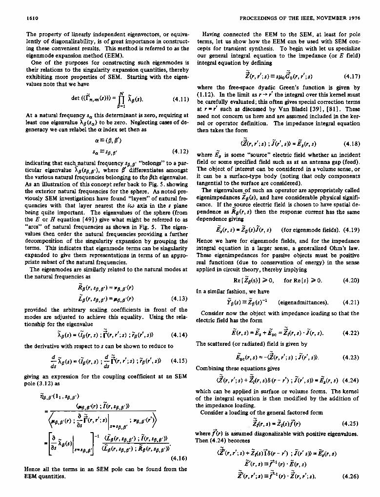
Having connected the EEM to the SEM, at least for pole terms, let us show how the EEM can be used with SEM concepts for transient synthesis. To begin with let us specialize our general integral equation to the impedance (or E field) integral equation by d e f i i g

Z(r, r’; s) = s p o &(r, r’; 8 )

5 - + (4.17)

where the free-space dyadic Green’s function is given by (1.12). In the limit as r + I‘ the integral over this kernel must be carefully evaluated; this often gives special correction terms at r = r’ such as discussed by Van Blade1 [391, [ 811. These need not concern us here and are assumed included in the kernel or operator definition. The impedance integral equation then takes the form

(Z(r, r‘; s) ; f(r‘, s)) = &(r, s) -

(4.18)

where is is some “source” electric field whether an incident field or some specified field such as at an antenna gap (feed). The object of interest can be considered in a volume sense, or it can be a surface-type body (noting that only components tangential to the surface are considered).

The eigenvalues-of such an operator are appropriately called eigenimpedances Zp(s) , and have considerable physical signifi- cance. If the-source electric field is chosen to have spatial dependence as Rp(r, s) then the response current has the same dependence giving

i S ( r , s) = .&(s)f(r, s) (for eigenmode fields). (4.19)

Hence we have for eigenmode fields, and for the impedance integral equation in a larger sense, a generalized Ohm’s law. These eigenimpedances for passive objects must be positive real functions (due to conservation of energy) in the sense applied in circuit theory, thereby implying

Re [ i?p(s)] 2 0, for Re [s] 2 0. (4.20)

In a similar fashion, we have

?p(s) .?p(s)-’ (eigenadmittances). (4.21) Consider now the object with impedance loading so that the

electric field has the form - E(r , s) =is + isc = &(r, 8 ) f(r, 8 ) .

- (4.22)

The scattered (or radiated) field is given by 5

2&, s) = -(&, r‘; s) ; f(r‘, s)). (4.23)

Combining these equations gives - - (Z(r , r ’ ; s ) + &(r, s)S (r - r’) ; f(/, s)) = i s ( r , s) (4.24)

which can be applied in surface or volume forms. The kernel of the integral equation is then modified by the addition of the impedance loading.

Consider a loading of the general factored form - ZLr, s) = Z&r) (4.25)

(4.26)


Defining modified eigenimpedances and modes as - ( 2 ( r , r ) ; s) ; ii; (rl, s)) = 2; ( 3 ) i p (r , s) - ( ~ $ ( r , s ) ; ?(r, r ’ ; s ) ) = i b ( s ) i ; ( r ’ , s ) (4.27)

we observe on substituting such modes into the modified integral equation (with impedance loading) that these modekare eigenmodes of the new equation with eigenvalues .?b(s) + Z,(s) which we summarize symbolically as

ir; ( r , s) impedance i; (r, $1 loading - i&, s) -q#, s)

“;,0%r

mpedance loading

q3 ( 8 ) - 2; ( 8 ) + i , ( s ) . (4.28)

For the case of 7 = (uniform loading) the unmodified eigenmodes and eigenimpedances appear in (4.28).

For synthesis now suppose we have computed z;(s) for some set of /3 values and plotted these in the complex s plane. The zeros of these eigenimpedances are natural frequencies sp,p’ of the antenna o r scatterer. Suppose we wish to change the natural frequencies to some new values to increase the damping, make the response more broad band, critically damp the dominant pole, or whatever. The basic synthesis equation is to choose Z,(s) such that

zl (s0,p’) = - Z b ( s p , p ’ ) -

(4.29)

at the desired set of s0,p’. Note that this is a set of explicit requirements on the loading to give certain desired features to the response.

As an example Tesche (in a private communication) has applied this method in MOM to form to synthesizing the transient response of a thin-wire antenna or scatterer. Fig. 14 shows the first two eigenimpedances for a uniformly loaded thin wire corresponding to the example case in Section 111-B. Note the natural frequencies (zeros) of the first eigenimpedance. Resistme loading corresponds to movement of the natural frequencies in the s plane along real negative (phase =br) values of the eigenimpedance. Note that the first conjugate pair of natural frequencies can be made to coalesce to give a secondader pole in the response on the negative_ s axis for critical damping by appropriate explicit choice of Z, as a positive resistance. These results are consistent with those obtained on a cut and try basis in a previous work [30] but give much more physical insight and a direct method. Note that for this wire problem the eigenimpe+ws luwa&saf ohms/ meter and are normalized by using Zo(s)L with units of ohms. This gives a result which is independent of wire length L if d/L is held constant.

Another type of frequencydomain modes is weighted eigenmodes of the form used by Garbacz and Turpin [ 571, [ 581 and by Harrington and Mautz [ 601. These are refeerred to as characteristic modes to distinguish them from the eigenmodes defined in (4.2). They have been shown to be useful for frequencydomain (CW) design and analysis of antennas and scatterers. These characteristic modes have some similar relations to the SEM quantities but appear to be more complicated for this purpose [ 881. More work is needed to further explore these relations.

900.

-4.0 -3.0 -2.0 -1.0 0 OL /c

z , ( s ) L ( in ohms) (a)

-4.0 -3.0 -2.0 - 1.0 0 rLL/C

Z p ( s ) L ( in ohms)

(b) Fig. 14. Lowest order,eigenimpedances zp(s) in the s plane for thin

wire, d /L = 0.01 (Tesche). p &dicates pole, z indicates-zero, and Z indicates saddle point. (a) Z, (s)L (in ohms). (b) Z,(s )L (in ohms).

V. FINITE-DIFFERENCE TIME-DOMAIN SOLUTIONS Previous sections have some ways to obtain transient infor-

mation from frequencydomain formulations. One might attempt to proceed directly in time domain without going through frequency domain. In particular Maxwell’s equations (1.4) are formulated as timedomain differential equations. Given some appropriate set of medium properties (permittivity, permeability, and conductivity), boundary conditions, initial conditions, and sources the problem can be numerically solved on large computers by the replacement of differential equations by corresponding difference equations.

While this approach is somewhat “brute force” in nature it does have some advantages. In particular it allows for the pres- ence of nonlinearities of the medium, boundaries, etc. which

1612 PROCEEDINGS OF THE EEE, NOVEMBER 1976

are described by differential equations and/or integrals over various quantities at times previous to the time the properties are required. The medium and boundaries can even be in somewhat arbitrary relative motion.

The typical procedure involves setting up some spatial grid of discrete points which may or may not be uniformly spaced and will typically conform to some convenient orthogonal curvilinear coordinate system. At some discrete time t , the electromagnetic and other quantities (such as electron density or whatever) are stored in the spatial array in the computer. The entries are updated to time t,,, = t , + At via the difference equations and other equations involving the previous values. This can be thought of as a time-marching process throughout the volume of interest. Various sophistications can be introduced such as converting the equations to retarded time and taking advantage of symmetries in the source and medium geometries.

This approach has been quite extensively applied to nonlinear plasma physics. In particular it has been the mainstay of studies of the generation of the nuclear electromagnetic pulse (EMP). In this problem there are compton and photoelectron source currents with electron trajectories determined by the fields, air conductivity from ionization and air chemistry reac- tion rates (involving electrons, ions, and neutrals), field dependent electron mobility, and various geometries such as proxim- ity to the earth surface and various scatterers. Numerous investigators have developed these calculations over more than the past decade and there is an extensive literature in the EMP theoretical notes on this subject. Some of the more prolific contributors to this area have been C. L. Longmire, W. J. K m a s , R. Latter, W. R. Graham, R. R. Schaefer, G. Schlegel, I. S. Malik, B. R. Suydam, J. H. Darrah, W. T. Wyatt, M. A. Messier, W. A. Radasky, H. J. Longley, E. D. Dracott, D. A. Moody, and J. J . Hill.

One of the significant problems with this approach is that of numerical errors which are often considered in the context of stability and convergence. It is very difficult to perform rigorous numerical analysis on these numerical schemes. Some attempts have been made in this direction, for example by Richtmyer 1381. In order to obtain good solutions at late time large amount of computation time is required.

Another problem this approach has been applied to is the penetration of high intensity magnetic fields (as in some EMP situations) through ferromagnetic shields. Some work of Merewether 1 43) , [ 441 is an example of this.

The finitedifference timedomain approach sheds little direct insight into the properties of the solution, such as by exhibiting various separate factors or terms in summations. However, for nonlinear problems such decomposition would appear to be much more limited. For such problems the finitedifference timedomain approach may not impose additional restrictions that are not inherent in the nature of the problem; this requires more investigation.

It may be possible to combine this approach with other approaches, such as time domain integral equations, with each approach handling a separate part of the problem. This would be analogous to the uni-moment method introduced by Mei [ 6 1 ] in frequency domain.

VI. TIME-DOMAIN INTEGRAL EQUATIONS

One of the recently developed approaches is the numerical solution of an appropriate timedomain integral equation de- scribing the response of an antenna or scatterer. As discussed

in Section I timedomain integral equations (integrodifferential equations) have the form

This can be converted into numerical form by MOM procedures noting that both space and time coordinates are to be discretized.

Since the operation over time is a convolution, involving current for previous time, the numerical solution considerably simplifies. If the time is sampled at some uniform At then we can write symbolically

+ I @ , t n ) (6.2)

where the term for tn involves evaluation of the operator with r ZL r' (i.e., a small space zone pound the point of obsemation) since the causal operator only perqits such a small zone to in- fluence I at t = t,. Inversion of r (r, r'; 0) gives the desired I(r, t ) in terms of its previous (and hence known) values. The detailed numerical procedures are somewhat more complicated and the reader is referred to various works which give detailed considerations to this numerical approach. Specifically numerous works of Bennett et al. 1621-1641, [66]-1681 and Liu I271 have developed this approach in detail. The reader may also consult books with review this subject, including the chapter by Poggio and Miller [ 12, ch. 41 and the chapter by Mittra 1 13, ch. 2) .

An interesting application of this type of numerical solution is to inverse scattering. As shown by Bennett (in a private communication) the shape of a perfectly conducting scatterer can be generated from the backscattefid signal for the case of axial incidence on an assumed body of revolution. While limited in scope this result does point in the direction of explicit inverse-scattering algorithms associated with a transient wave form detected at some point in space.

It would be interesting to know some of the inherent properties of the timedomain integral equations analogous to the singularity expansion and the eigenmode expansion developed for frequencydomain integral equations. Once can defiie an eigenmode equation corresponding to (4.1) where now integration is over space and time. The resulting eigenmodes and eigenvalues appear to be related to SEM and EEM quantities, but this is a subject for future investigations.

VII. APPROXIMATE TRANSMISSON-LINE MODELS OF THIN ANTENNAS AND SCATTERERS

It is sometimes useful to formulate crude physical models of antennas and scatterers that are not very accurate but give significant physical insight and simplicity. If simple explicit formulas for the response are obtained these formulas can be used in a synthesis or design sense to obtain desired performance.

One such approximation applies to thin antennas and scatterers in the form of a one dimensional approximation which can be thought of as a transmission-line form. This type of approximation has been shown to be useful for transient thin-wire radiators of the form in Fig. 11 1 191, [33]. However, other thin-wire structures can also be analyzed by such an approach.


E (5,s) incident or source field

i ( C . s ) impedance loading per unit length

(a)

C'(C 1 dC

- - - T--- postulated reference surface

(b) Fig . 15. Transmission-line model of antenna. (a) Wire antenna or

scatterer. (b) Incremental section of transmission-line model.

For this purpose an incremental section of the wire structure is assumed to be modeled by a series inductance pEr unit length L '( f ) and loading impedance per unit length A( f , s) and by a transverse capacitance per unit length C'({) as illustrated in Fig. 15. There may also be a distributed source ig the form of an incident electric field with component E , ( { , s) parallel to the wire. In order to define L' and C' one postulates some imaginary reference surface which serves as the outer conductor for a coaxial transmission line. The center conductor is the wire (say of radius u ) with some position variable f which varies along the wire. Note that radiation resistance is not included in this model.

In terms of these parameters one can define a characteristic impedance for the wire as

with the constraint that the propagation velocity along the wire (in free space) in the absence of loading be the speed of light as

1 c=d-'

In determining L' and C' it is often more convenient to consider Z , using some assumed outer conductor radius (coaxial model) or the characteristic (pulse) impedance of an appropriate biconical antenna which approximates the wire [6]. As an example the thin-wire antenna of radius u and half- length h driven at the center (see Fig. 11) has a characteristic impedance (for smaUu/h) [ 191

z,==%(F). 277 (7.3)

Using this formalism one -.obtain cbaa&hm solutions for currents on the wire an teqa or scatterer for special variations of Z,(f) (shape) and A({, s) (impedance loading) such as one might be concerned with in the study of non- uniform transmission-line transformers. King, Wu, and Shen [82], [83] have discussed a particular form of impedance loading which gives a nonreflecting type of current wave on

a thin cylindrical antenna. Using that type of resistive loading distribution with a simplified transmission-line model one can obtain a simple solution for the current and radiated fields if the coefficient of the resistance function is appropriately constrained [ 191. For other values of the resistance (but the same ( h - z)-' spatial dependence) more complicated formulas are obtained [331.

One deficiency of this transmission-line model is its lack of damping of transient response waveforms if there is no resistive impedance loading. This illustrates the importance of the wire being thin which has small damping in fact. For cases of significant resistive loading (say to achieve critical damping) the model is somewhat better. For more accurate estimates of thin-wire response one can use an asymptotic theory ( a + 0) which has transmission-line characteristics only as the leading term [ 591 .

VIII. CLOSED FORM TRANSIENT SOLUTIONS FOR SPECIAL GEOMETRIES

There are some special types of geometries which admit of exact and explicit transient solutions. Consider first some usual geometries which admit of separation-of-variable solutions for electromagnetic scattering in frequency domain. By inverse Laplace transformation the series of terms in the solution can be converted into a series of time-domain terms. For example scattering of a plane wave by a perfectly conducting sphere [45] and by a perfectly conducting cylinder [42], [ 871 have been treated this way. An infinite cylindrical antenna driven by a delta (slice) gap also admits a closed form transient solution [ 181, [ 201 -[ 221, [ 781 . One can also solve scattering by a perfectly conducting wedge in explicit form [13,ch. 1 1 , ~ 1 6 1 , ~ 2 4 1 , ~ 3 5 1 , ~ 7 8 1 . For transient field production for testing of various objects,

as in the case of the nuclear electromagnetic pulse [ 141, [ 151, [26], the TEM mode of cylindrical and conical transmission lines is used extensively to produce fields with a constant waveform (dispersionless) throughout some volume of space. A cylindrical transmission line as illustrated in Fig. 16(a) has a TEM mode characterized by an electric-field distribution [71, [ 141, [251.

E(r , t ) = E o [Vt@(x,v)l f(t * z / c ) (8.1)

where fz is the direction of propagation, f is the waveform, Vi- is the transverse gradient, and Eo is a scaling constant. Similarly a conical transmission line has a TEM mode (trans verse with respect to r ) as [ 151

~ ( r , t ) = - [ V t W , @)I f ( t f r k ) . V O r (8.2)

Conical transmission lines as in Fig. 16(b) with small taper angles (conductors within a small angle based on the apex, r=.fl) can be approximately matched to cylindrical trans mission lines to launch and/or terminate the TEM mode thereon [ 151 . This important property of such structures allows the construction of EMP simulators with very convenient field properties as in (8.1) over an extremely wide band of frequencies (including down to dc or s = 0).

Objects such as cylindrical (or conical) transmission lines also have higher order (E and H ) modes (leaky modes) which have more complicated properties in that they are dispersive and do not maintain a transient waveform independent of z , the longitudinal coordinate. These modes have been com-

1614

\ Y

(b) Fig. 16. TEM transmiasion lines. (a) Cylindrical transmission line.

(b) Conical trammission line.

puted for open cylindrical transmission lines and used to &e transient propagation thereon [ 291, [34] , [37]. These modes are similar to the classical modes for closed waveguides except that they decay in the direction of propagation and grow in the transverse direction away from the transmission line.

IX. SUMMARY While transient and broad-band electromagnetics has seen

some considerable recent interest and development and has developed a considerable literature, it would appear to still be somewhat in its infancy as far as what technology is needed and likely to be developed. The results currently available range from simple but approximate formulas which give considerable physical insight 1361 to sophisticated analytical tools of a more exact nature [ 131.

Both analytical and numerical methods have been developed but one should not look at these as being completely disjoint. Analytical and numerical methods can be hybrided together for better physical insight as well as numerical efficiency and accuracy.

The interim nature of the current technology should be emphasized, but already some of the ideas for a more com- plete technology are coming forward. More ideas are yet to be developed and implemented but it would seem that some of the -likely sources of these can be identified including adaptation of various CW concepts, application of concepts from physics (quantum mechanics), and development of concepts from the early sources of electromagnetic theory which have laid dormant for lack of applications in the past. The field is moving rapidly ahead and it appears that one or more synthesis procedures for transient antennas and scatterers will be thoroughly developed, thereby converting the subject into a true engineering discipline. Already numerous special types of antennas for radiating or controlling eansient/broad- band fields and other types for measuring them have been

PROCEEDINGS OF THE IEEE, NOVEMBER 1976

developed. However, the consideration of the details of these various designs is beyond the scope of this paper. Already some of the new methods are leading to equivalent circuit representations for antennas and scatterers [ 901 , [ 9 1 ] .

This paper has dealt primarily with concepts in the field of transient and broad-band electromagnetics. The detailed application of these can be quite involved and for this and for the numerical details the reader is referred to the literature.

REFERENCES

In the interest of brevity the following abbreviations are used:

SSN Sensor and Simulation Notes TN Theoretical Notes IN Interaction Notes

MaN Mathematics Notes

These are part of the note series on EMP and related subjects described in “The Compleat Guide to the Notes,” INDEX 1-1 , February 1973, by this author. These have played a promi- nent role in transient/broad-band technology. Listings of these can also be found in the IEEE AP-S Newsletter. Copies of these papers can be requested from the author, from the Defense Documentation Center, Cameron Station, Alexandria, VA 22314, or from the Editor, Dr. Carl E. Baum, Air Force Weapons Laboratory (EL), Kirtland AFB, NM 87117. In addition these notes are available at many universities and companies doing research in EMP and electromagnetic theory. Where known, cross-reference to other articles based on such notes are included. The reader’s attention is particularly directed at the book edited by Felsen [ 131 as a general reference to the subject of this paper. The following reference list is not exhaustive, since every reference related to transient electromagnetics would give a huge list. (The notes on EMP and related subjects are already approximately one thousand in number.)

J. C . Maxwell, A Treatise on Electricity and Magnetism (2 vols.)

H. Hertz, Electric Waves, D. E. Jones, Transl. New York: Dover, 1954 (from 3rd ed., 1891).

0. Heaviside, Electromagnetic Theory. New York: Dover, Dover, 1962 (from 1893 ed).

1950, (from 3 vols., 1893,1899, and 1912).

Hill, 1941. J. A. Stratton, Electromagnetic Theory. New York: McGraw-

E. T. Whittaker, A History of the m o r i e s of Aether and Elec- tdcity (2 vols.), New York: Humanities Press, 1973 (from

S. A. Schelkunoff and H. T. Friis, Antennas: Theory and Prac- 1951 ed).

tice. New York: Wley, 1952.

Hill, 1960. R. E. Collin, Field m o r y of Guided Waws. New York: McGraw-

J . VanBladel, EIeceomagnetic FieMs. New York: McGraw- Hill, 1964. M . Abramowitz and I. A. Stegun, Eds., Handbook of Mathe- matical Functions. Washington, DC: US. Gov’t. Printing Office, 1964.

New York: Macmillan, 1968. R. F. Harrington, Field Computation by Moment Methods.

C. T. Tai, Dyodic Green’s Functions in Electromagnetic Theory. New York: Intext, 1971. R. Mittra Ed., Computer Techniques for Electromagnetia. New York: Pergamon, 1973.

Chapters 1. R. Mittra, “A brief preview.” 2. G. A. Thiele, ‘Wire antennas.” 3. P. C. Waterman, “Numerical solution of electromagnetic

4. A. J. Poggio and E. K. Miller, “Integral equation solutions

5. C. P. Wu, ‘Yariationd and iterative methods for waveguides

6. R. Mittra and T. Itoh, “Some numerically efficient methods.” 7. R. Mittra, “Inverse scattering and remote probing.”

scattering problems.”

of three-dimensional scattering problems.”

and arrays.”


[ 131 L. B. Felsen Ed., Transient Electromagnetic Fields. New York: Springer-Verlag, 1975.

Chapters 1. L. B. Felsen, “Propagation and diffraction of transient

2. R. Mittra, “Integral equation methods for transient

4. D. L. Sengupta and C. T. Tai: “Radiation and reception 3. C. E. Baam, “The singularity expansion method.’‘

(14) C. E. Baum, “Impedances and field distributions for parallel 5. J . A. Fuller and J. R. Wait, “A pulsed dipole in the earth.”

[ 15) -, “The conical transmission line as a wave launcher and plate transmission line simulators,” SSN 21, June 1966.

terminator for a cylindrical transmission line,” SSN 31, Jan. 1967.

[ 161 -, “The diffraction of an electromagnetic plane wave at a bend in a perfectly conducting planar sheet,” SSN 47, Aug. 1967.

[ 171 -, “A scaling technique for the design of idealized electromag-

fields in nondisperaive and dispersive media.”

scattering.”

of transients by linear antennas.

netic lenses,” SSN 64, Aug. 1968. 181 R. W. Latham and K. S. H. Lee, “Pulse radiation and synthesis

by an infinite cylindrical antenna,” SSN 73, Feb. 1969. (Also as R. W. Lantham and K. S. H. Lee, “Transient properties of an i n f d t e cylindrical antenna,” Radio Sci., vol. 5, pp. 715-723, Apr. 1970.)

191 C. E. Baum, “Resistively loaded radiating dipole based on a transmissionhe model for the antenna,” SSN 81, Apr. 1969.

201 R. W. Latham and K. S. H. Lee, “Radiation of an infinite cylindrical antenna with uniform resistive loading,” SSN 38, Apr. 1969.

211 -, “Waveforms near a cylindrical antenna,” SSN 89, June 1969.

[22] L. Marin, “Radiation from a resistive tubular antenna excited by a step voltage,” SSN 101, Mar. 1970. (Also as L. Marin, “Tran- sient radiation from a resistive, tubular antenna,” Radio Sci., vol. 9, pp. 631-638, June 1974.)

[23] C. E. Baum, “Some characteristics of electric and magnetic antennas for radiating transient pulses,”SSN 125, Jan. 1971.

I241 D. F. Higgins, “The diffraction of an electromagnetic plane wave by interior and exterior bends in a perfectly conducting sheet,”SSN 128, Jan. 1971.

[: 2 5 1 C. E. Baum, “General principles for the design of ATLAS I and 11,

waveforms launched by imperfect pulser arrays onto TEM part V: Some approximate ftgures of merit for comparing the

transmission lines,” SSN 148, May 1972. 261 C. E. Baum, EMP simulators for various types of nuclear EMP

environments: an interin categorization,” SSN 151, July 1972. 271 T. K. Liu, “Direct time-domain analysis of linear EMP radiators,”

SSN 154, July 1972. 281 T. C. Mo, C. H. Papas, and C. E. Baum, “Differential geometry

scaling method for electromagnetic field and its applications to coaxial waveguide junctions,” SSN 169, Mar. 1973. (Also as T. C. Mo, C. H. Papas, and C. E. Baum, “General scaling method for electromagnetic fields with application to a matching prob-

291 L. Marin, “Transient electromagnetic properties of two parallel lem,” J. Math. Phys.,vol. 14, pp. 479-483, Apr. 1973.)

wires,” SSN 173, Mar. 1973. 301 F. M. Tesche, “Application of the singularity expansion method

to the analysis of impedance loaded linear antennas,” SSN 177, May 1973. (Also as F. M. Tesche, “The far-field response of a stepexcited linear antenna using SEM,” B E E Trans. Antenmu

311 C. E. Baum, “Singularity expansion of electromagnetic fields and potentials radiated from antennas or scattered from objects in free soace.” SSN 179. Mav 1973.

P r o p ~ a t . , V O ~ . AP-23, pp. 834-838, NOV. 1975.)

[ 321 T. H. S h u m k , “EMP intiraction with a thin cylinder above a ground plane using the singularity expansion method,” SSN

and D. R. Wilton, “Scattering by a thin wire parallel t o a ground 182, June 1973. (Also as K. R. Umashankar, T. H. Shumpert,

AntennasPropagat.,vol. AP-23, pp. 178-184, Mar. 1975.) plane using the singularity expansion method,” IEEE Tram

[33] D. L. Wright and J. F. Prewitt, “Transmission line model of radiating dipole with special form of impedance loading,” SSN 185, September 1973. (Also as D. L. Wright and J . F. Prewitt,

IEEE Trans. Antennas Propagat., vol. AP-23, pp. 811-814, Nov. “Radiating dipole antenna with tapered impedance loading,”

1975.) [34] L. Marin, “Modes on a fiite-width, parallel-plate simulator I:

Narrow plates,” SSN 201, Sept. 1974. [ 351 K. K. Chan, L. B. Felsen, S. T. Pew, and J. Shmoys, “Diffrac-

tion of the pulsed field from an arbitrarily oriented electric or

[36] G. Franceschetti and C. H. Papas, “Pulsed antennas,” SSN 203, magnetic dipole by a wedge,” SSN 202, Oct. 1973.

Dec. 1973. (Also as G . Franceschetti and C. H. Papas, “Pulsed antennas,” ZEEE Trans. Antennas Propagat., vol. AP-22, pp. 651-661, Sept. 1974.)

[ 371 T. Itoh and R. Mittra, “Analysis of modes in a fmite-width parallel-plate waveguide,” SSN 208, Jan. 1975.

[38] R. D. Richtmyer, “Stability of the new radio flash code,” TN 126, Aug. 1967.

[39] K. S. H. Lee and L. Marin, “Interaction of external system- generated EMP with space systems,” TN 179, Aug. 1973. (Also as K. S. H. Lee and L. Marin, “Charged particle moving near a perfectly conducting sphere,” IEEE Trans. Antennu? Propagat., VOl. AP-22, pp. 683-689, Sept. 1974.)

(411 C. E. Baum, “Interaction of ekctromagnetic fields with an 140) -, “SGEMP for resonant structures,” TN 199, Sept. 1974.

object which has an electromagnetic symmetry plane,” IN 63,

[42] P. R. Barnes, “The axial current induced on an infinitely long, Mar. 1971.

perfectly conducting, circular cylinder in free space by a transient electromagnetic plane wave,” IN 6 4 , Mar. 1971.

[43] D. E. Merewether, “Analysis of the shielding characteristics of saturable ferromagnetic cable shields,” IN 67, Aug. 1970. (Also as D. E. Merewether, “Analysis of the shielding characteristics of saturable ferromagnetic cable shields,” ZEEE Tram Elec-

[44] -, “Design of shielded cables using saturable ferromagnetic tromagn. Comprrt.,vol. EMC-12, pp. 134-137, Aug. 1970.)

materials,” IN 68, Aug. 1970. (Also as D. E. Merewether, “De-

IEEE Trans. Eiectromagn. Compat., vol. EMC-12, pp. 138-141, sign of shielded cables using saturable ferromagnetic materials,”

Aug. 1970. [45] C. E. Baum, “On the singularity expansion method for the

solution of electromagnetic interaction problems,” IN 88, Dec.

[46] L. Marin and R. W. Latham, “Analytical properties of the field 1971.

scattered by a perfectly conducting, f d t e body,” IN 92, Jan. 1972. (Also as L. Marin and R. W. Latham, “Representation of

Proc. ZEEE, vol. 60, pp. 6440-641, May 1972; and L. Marin, transient scattered fRlds in terms of free oscillations of bodies,”

“Natural-mode representation of transient scattered fields,” IEEE Thms. Antennas Propagat., vol. AP-21, pp. 809-818,

[47] F. M. Tesche, “On the singularity expansion method as applied Nov. 1973.)

53

54

t o electromagnetic scattering from thin-wires,” IN 102, Apr. 1972. (Also as F. M . Tesche, “On the analysis of scattering and antenna problems using the singularity expansion technique,” IEEE Trans. AntenMs Propagat., vol. AP-21, pp. 52-63, Jan. 1973).

481 L. Marin, “Application of the singularity expansion method to scattering from imperfectly conducting bodies and perfectly conducting bodies within a parallel plate region,” IN 116, June 1972.

491 L. Marin, “Natural-mode representation of transient scattering

numerical results for a prolate sphere,” IN 119, Sept. 1972. from rotationally symmetric, perfectly conducting bodies and

scattering from rotationally symmetric bodies,” IEEE Trans. (Also as L. Marin, “Natural-mode representation of transient

501 S. W. Lee, V. Jamnejad, and R. Mittra, “An asymptotic series Antenmu Propagat., vol. AP-22, pp. 266-274, Mar. 1974.)

for early time response in EMP problems,” IN 128, Oct. 1972. (Also as S. W. Lee, V. Jamnejad, and R. Mittra, “An asymptotic series for early time response in transient problems,” lEEE me. Antenmu Propagat., vol. AP-21, pp. 895-899, Nov. 1973.)

5 1 1 C. E. Baum, “On the singularity expansion method for the case

521 P. R. Barnes, “On the singularity expansion method as applied of fust,order poles,” IN 129, Oct. 1972.

to the EMP analysis and simulation of the cylindrical dipole antenna,” IN 146, Nov. 1973.

] D. R. Wilton and K. R. Umashankar, ‘Tarametric study of an L-shaped wire using the singularity expansion method,” IN 152, Nov. 1973. (+ as K. R. Umashanakar and D. R. Wilton,

expansion method,” iEEE Thms. Antenna8 Propagat., vol. “Transient scattenng of an Lghaped wire using the singuMty

1 T. T. Crow, B. D. Graves, and C. D. Taylor, “The singularity

in free space,” IN 161, Oct. 1973. (Also as T. T. Crow, B. D. expansion method as applied to perpendicular crossed cylinders

Graves, and C. D. Taylor, “The singularity expansion method as applied to perpendicular crosed wires,”ZEEE Trans. Antennas

AP-23, pp. 838-841,Nov. 1975.)

ProPogot., VOf. AP-23, pp. 540-546, July 1975.) 1551 K: R. Umashankar and D. R. Wilton, “Andy& of an L-shaped

wire over a conducting ground plane using the singularity expansion method,” IN 174, Mar. 1974.

1561 C. D. Taylor, “A simple procedure for estimating the current induced on cylinder-like conductors illuminated by a unit step electromagnetic pulse,” IN 176, July 1973.

I571 R. J. Garbacz, “A generalized expansionforradiated and scattered fields,” IN 180, 1968.

I581 R. H. Turpin, “Basis transformation, least square, and characteristic mode techniques for thin-wire scattering analysis,” IN


eralized expansion for radiated and scattered fields,”LEEE Trans 181, 1970. (Also as R. J. Garbacz and R. H. Turpin, “A gen-

(591 L. Marin, ‘‘Natural modes of certain thin-wire structures,” IN Ante- Ropagat., vol. AP-19, pp. 348-358, May 1971.)

(601 R. F. Harrington and J. R. Mautz. “Theory and computation of 186, Aug. 1974.

characteristic modes for conducting bodieq” IN 195, Dec. 1970.

teristic modes for conducting bodies,” BEE 7hmz Antennas (Also as R. F. Harriugton and J . R. Mautz, “Theory of charac-

Hwington and J . R. Mautz, “Computation of characteristic modes for conducting bodies,” LEEE Tram Antennas Ropagat.,

(61 1 K. K. Mei, “Uni-moment method of solving antenna and scattering problems,” IN 205, Sept. 1973. (Also as K. K. Mei, “Uni-

lEEE Tnar Antennas Pmpagut., vol. AP-22, pp. 760-766, Nov. moment method of solving antenna and scattering problems,”

1974.) [62] C. L. Bennett, Jr., and W. L. Weeks, “A technique for computing

bodies,’’ IN 222, June 1968. (Also as C. L. Bennett, Jr., and approximate electromagnetic impulse response of conducting

LEEE Tmns. Antenmu Promat. , vol. AP-18, pp. 627-633, W. L. Weeks, “Tranrient scattering from conducting cylinders,”

Sept. 1970.) (631 C. L. Bennett, J . D. DeLorenzo, and A. M. Auckenthakr, “In-

tegral equation approach to wideband inverse scattering: Volume

June 1970. I, Development of procedum for numerical solution,” IN 226,

(641 -, “Integral equation approach to wideband inveme scattering: Volume 11, Computer program descriptions and listings,” IN 227, June 1970.

[65] C. E. Baum, “On the eigenmode expansion method for electro-

relations for eigenmode expansions and their relation to the magnetic scattering and antenna probkms, part I: some basic

singularity expansion,” IN 229. Jan. 1975. (661 R. S. Smith, J. D. DeLorenzo, and C. L. Bennett, ‘“elwrements

of and d i su imht ion with smoothed i m p w rcrpom of r d a r targets,” IN 232. Nov. 1970.

[67] c. L. Bennett, A. M . Auckenthaler, R. S. Smith, and J. D. Dehrenzo, “space time,ptegral equation approach to the lugs body scattering problem, IN 233, Jan. 1973.

(681 C. L. Bennett. K. S; Meager, R Histonymus. J. D. DeLorenzo, and D. Anderson, Space time integral equation approach for targetswith edges,”IN 234, July 1974.

I691 M. L. VanBlaricum and R. Mittra, “A technique for extracting the poles and residues of a system directly from its transient response,” IN 245, Feb. 1975. (Also as M. L. VanBlaricum and R. Mittra, “A technique for extracting the poles and residues of a system directly from its transient response,’’ LEEE lhnr AnteMarRopagat., vol. AP-23, pp. 777-781, Nov. 1975.)

[70] F. M. Tesche, M. A. Morgan, B. Fishbine, and E. R. Parkinson,

model improvements,” IN 248, July 1975. “Internal interaction analysis: topological concepts and needed

[71] F. J . Sulkowski, “FORPLEX, a program to calculate inverse Fourier transforms,’’ MaN 2. Nov. 1966.

I721 T. T. Crow, B. D. Graves, and C. D. Taylor, “Numerical tech-

Propagat., VO~. AP-19, pp. 622-628, Sept. 1971; and R. F.

VOl. AP-19,pp. 629-639, Sept. 1971.)

niques useful in the singularity expansion method as applied to electromagnetic interaction problems,” MaN 27, Dee. 1972.

[73] C. E. Baum, “On the use of contour integration for finding poles, zeros, saddles, and other function values in the singularity

(741 C. 0. Beasley, Jr., and H. K. Meier, “Subroutine CAUCHY: expansion method,” M a N 35, Feb. 1974.

complex roots of a function using a Cauchy integral technique,” M a N 37, Aug. 1974.

[75] B. K. Singaraju, D. V. Giri, and C. E. Baum, “Further develop ments in the application of contour integration to the evaluation of the zeros of analytic functions, and relevant computer pro- grams,” MaN 42, Mar. 1976.

[ 761 L. B. Felsen and G. A. Deschamps, guest e&, Roc. EEE (Special h e on Rays and Beams),vol. 62, Nov. 1974.

[77] Lord Rayleigh, “On the incidence of aerial and electric wavea upon sml obstacles in the form of ellipsoids or eIliptic cylindera, and on the p ~ l a g e of electric waves through a circular aperture

(781 C . H. Papas, “On the infinitely long cylindrical antenna,” J. in a conducting saeen,”PhfL Mag.,vol. 44. pp. 28-52, 1897.

I791 J . B. Kener and A. Blank, “Diffraction and reflection of pubes

pp. 75-94.1951. by wedges and cornen,” Commn. Rue a.nd Appl. Math., vol. 4.

(801 A. F. Stwenson, “Solution of electromagnetic scattering problems aa power series in the ratio (dimendon of scatterer)/wave-

I811 J. VanBlrdel, “Some remarks on Green’s dyadic for infinite length,”J. AppL Phyr., vol. 24, pp. 1134-1 142, Sept. 1953.

space,” IRE Tmna. A n a m Propagat., vol. Ap-9, pp. 563-566,

(821 T. T. Wu and R. W. P. King, ‘The cylindrical antenna with nom Nor. 1961.

reflecting nrtttke loading,” BEE Tram Antennaa Pmpagat., vo1. AP-13, pp. 369-373, May 1965.

(831 L. C . Shen and R. W. P. King, ‘The cylindrical antenna with nonreflecting resistive loading,”LEEE Tmns. AnanmwPropqyt.,

( 8 4 ) R. E. Kleinman, “Low frequeney mlution of electromagnetic scattering problems,” in J. Brown, Ed., ElectromrgncUc Wmre Theory. New York: Pergamon, 1967.

(851 R. E. Kleinman and T. B. A. Senior, “Low-frequency scattering by space objects,’’ IEEE Tnar Aerospace Elcc. Syr., vol. AES

[86] D. L. Moffatt and R. K. Mains, “Detection and disahninrtion of radar targets,” LEEE lktw. Antennas Pmpagat., vol. AP-23, pp. 358-367, May 1975.

(871 R. H. Schafer and R. G. Kouyoumfian, “Transient currents on

A n t e m Ropagat., vol. AP-23, pp. 627-638, Sept. 1975. a cylinder illuminated by an impulsive plane wave,”LEEE ”hm

I881 C. E. Baum, “Introduction t o SEM,” preosnted at 1973 GAP

[89] -, “HOW to think about EMP interaction,” in Roc. I974 International Symposium and USNC/URSI Meeting, Aug. 1973.

S p h g FULMENMeet., pp. 12-23, Apr. 1974. [90] -., “Use of singularities in the complex plane and eigenvalues

of mtegral equations for translent and broadband electromagnetic analysis and synthesis,” presented 1975 APS International Symp. and USNC/URSI Meeting, June 1975.

91 ] -, “SingIe port equivalent circuits for antennas and scatterers,” IN (to be published).

AppL Phyr., VOL 20, pp. 437-440, 1949.

VOl. AP-13, p. 998, NOV. 1965.

11, pp. 672-675, July 1975.

broadlband analysis and synthesis of antennas and scattererssaito/data/sonar/baum-iproc.pdf ·...

Documents