1

Forthcoming In I. Vaccaro, E. A. Smith, and S. Aswani (eds.) Environmental Anthropology: Methodologies and Research Design. Cambridge, UK: Cambridge University Press.  Spatial‐temporal  methodologies  in  Environmental  Anthropology:  Geographic Information Systems, remote sensing, landscape changes and local knowledge.  Brondizio, E.S. and R. Roy Chowdhury. Indiana University  Introduction Spatial  tools  such  as  remote  sensing  (RS)  and  geographic  information  systems  (GIS)  are increasingly used in a variety of research applications. The popularization of geospatial data and tools  in the media and society has significantly changed the way we perceive, understand and manage  our  landscapes.  A  variety  of  social  actors  have  become  familiar  with  these technologies, whether  they  be  an  extractivist  cooperative  disputing  borders  in  the  Brazilian Amazon,  a US  resident  checking his property  in  cadastral map, or  a  school  teacher  in  India, using  a  satellite  image  to  teach  regional  geography.  Today,  geospatial  technologies  are recognized  as  valuable  assets  of  civil  society  and  essential  tools  to  address  social  and environmental  problems  (NAS  2002).  The  proliferation  of  satellite  and  public‐domain  spatial data, Global Positioning Systems (GPS), affordable computer hardware and software, and data processing  and  analytical  techniques  continue  to  expand  the  use  of  these  technologies  in anthropology generally, and environmental anthropology in particular. Such spatial information is frequently used in visualization (e.g., displays of aerial photography or satellite imagery for a study region) using Google Earth or other public domain software that allow quick online data access/display  without  requiring  specialized  training.  More  in‐depth  research  and  analyses entail  the  use  of  designated  RS/GIS  software  programs  (e.g.,  ERDAS  Imagine,  ArcGIS,  Idrisi, Multispec,  among many  others),  and  the  actual  acquisition  of  the  relevant GIS  datasets  (as opposed to merely accessing them for online displays and/or simple queries).    This chapter reviews uses and issues in the application of RS and GIS in anthropological research. We briefly review fundamental geospatial concepts and provide a concise history of RS and GIS applications in Anthropology. Next, we present the range of geospatial concerns in anthropological research design, highlighting research questions, units of analysis, data search and  temporal  sampling,  and  assessments of data processing needs  and  analysis.  In order  to illustrate these geospatial concerns, we focus in particular on land use/cover change research, and provide guidelines for data planning and research design. Finally, we present critical ethical and pragmatic issues in the (re)presentation of spatiotemporal data and maps, reflecting on the positive potential as well as perils of using these tools in anthropological research.  Fundamentals of remote sensing and GIS RS, GIS and GPS are complementary suites of geospatial technologies and methods, collectively implicated in GIScience (Jensen 1996; Goodchild and Janelle 2004). RS involves the collection of surface  reflectance  data  from  a  distance,  such  as  in  analog/digital  aerial  photography  or satellite  imagery  recording  information  about  the earth  surface  in  gridded  (raster) products. These data constitute the most significant sources of quantitative information about land cover 

2

and land use changes in the tropics and elsewhere (Sader et al., 1994). GIS, on the other hand, involve hardware,  software, database  systems  and methods  for  the  storage,  representation, processing, integration and analysis of diverse spatial data and their attributes. Both spatial and nonspatial  information may be recorded  in raster data or vector features such as points,  lines and polygons, referenced to a common cartographic system of spatial location. GIS enable the collation and processing of RS products for further representational or analytical tasks, such as modeling  deforestation  by  linking  data  on  forest  (change)  patterns  with  ancillary,  spatially explicit socioeconomic variables. The following sections briefly review key elements of RS and GIS. 

Remote sensing technologies enable the mapping of the earth’s surface and subsurface features  based  on  their  differential  reflectance  of  incident  electromagnetic  energy.  A fundamental  distinction  among  remote  sensing  technologies  is  based  on  the  source  of  that energy: passive sensors record reflectance of incident solar radiation (i.e., the energy source is independent  of  the measurement  device,  exemplified  by  optical  systems  such  as  Landsat), while active  sensors  record  the  return of wavelengths generated by  the  sensor  system  (e.g., microwave RADAR or LiDAR). Since the military surveillance systems of World War  II, sensors have  improved  to  capture  reflectance  in  a wider  range  of  optical wavelengths with  greater resolution, for progressively more information content. The level of detail (resolution) in digital imagery  can  be  related  to  at  least  three  aspects:  spatial,  spectral  and  radiometric.  These resolutions trade off with each other, and with the overall areal extent covered by each image scene/snapshot.  Spatial  resolution  refers  to  the  size  of  individual  pictoral  elements  (pixels), corresponding  to  rectangular  portions  of  the  earth  surface  being  imaged.  Higher  spatial resolution systems such as  IKONOS or Quickbird map earth surfaces  in great detail, with sub‐meter  pixels.  Spectral  resolution  refers  to  the  precision  with  which  sensors  partition  the electromagnetic spectrum  (into “bands”) to record reflectance. The human eye  is sensitive to wavelengths  in  the  visible  range,  or  300‐750nm  (blue  to  red wavelengths).  NASA’s  Landsat Thematic Mapper  sensor  system  captures  the  visible  range  in 3  ranges or  reflectance bands (blue,  green  and  red),  and  additionally  records  reflectance  in  four  infrared  bands  (three mid/near  infrared and one  thermal), as opposed  to up  to 220 bands  in hyperspectral remote sensing  (NASA’s  EO‐1  Hyperion  sensor).  Radiometric  resolution  refers  to  the  levels  of quantization  (referred  to  as  bit  depth) with which  the  sensor  captures  spectral  reflectance intensities  in a pixel, typically ranging from 0 to 255 (8 bits). Additionally, temporal resolution refers to the revisit frequency of the sensor for a specific point on the earth. Landsat TM has a temporal  resolution of 16 days, compared  to  the NOAA AVHRR satellite’s  twice‐daily  imaging frequency. Processing satellite imagery or digital aerial photographs of varying spatial, spectral and  radiometric  characteristics  involves  three  essential  steps:  geometric  correction (georeferencing),  radiometric  correction  (noise  removal) and various methods of  information retrieval relevant to the chosen application or research question. Subsequent sections (V) will discuss  some  of  these  image  processing  techniques  utilized  in  anthropological  research  on landscape characterization and change detection. Most RS applications, however,  involve  the analysis of RS‐derived data with GIS tools.  

Geographic information systems center on linked spatial and attribute (nonspatial) data, structured  within  a  chosen  model  to  represent  real‐world  spatial  objects  and  relations. Typically, GIS data models are of  two basic  types:  raster and vector. Raster data  represent a 

3

space‐filled, field‐based view, in which the geographic world is made up of continuously varying data values in gridded layers covering a study region. Spatial and attribute data are embedded within  the  same  data  structure:  the  spatial  grid  is  divided  into  square/rectangular  units, typically  of  uniform  dimensions,  each  cell  recording  qualitative  or  quantitative  attributes  of interest (e.g., land use codes, distance to nearest road network, degree of fire risk, etc.). Vector data,  on  the  other  hand,  subscribe  to  a  feature‐based  view  of  the world,  recording  precise boundaries and  information about  specific objects of  interest,  rather  than all  space within a study area. Three  types of  features  typically used are points  (e.g., houses),  lines  (e.g.,  roads) and polygons (e.g.,  land parcels). In a vector data model, spatial and attribute data are stored separately but linked through a common identifier, often within a relational database.  

The  development  of  modern  GIS  was  application  driven,  and  dates  to  the computerization  of  spatial  data  management  tasks  in  the  US  Census  and  Canadian  Land Inventory during  the 1960s. GIS software offer  tools  for spatial and  relational data entry and storage (including coordinate and attribute data capture or  importation), representation (e.g., through  various  data  models),  transformation  and  management  (e.g.  projections,  editing, reduction/summarization),  and  visualization  (various  output  formats  and  symbolization, alternate/dynamic  renderings of 2 or 3‐dimensional products, often embedded with  internet mapping). Most  significantly,  GIS  techniques  enable  the  integration  of  data  from  disparate sources,  and  the  analysis  of multiple  spatial  data  layers.  Analytical  tools  range  from  simple querying, distance and buffering  tools,  to map algebra and  spatial  statistics/interpolation, as well  as  complex  network/topological/terrain  analyses,  multi‐criteria  evaluations  and environmental  modeling.  Several  of  these  techniques  entail  the  integration  of research/methodological approaches as well as diverse data sources such as ethnographies and field‐derived surveys, cadastral information, digital elevation models, satellite or station derived climate  data,  land  cover  information,  or  utilities  and  infrastructure  networks.  These characteristics  explain  the  increasing  use  of  GIS  in  research  and  planning,  as  well  as environmental  and  spatial  decision‐making.  GIS  are  embedded,  however,  within  a  broader theoretical framework of GIScience, drawing from geospatial technologies (RS, GIS, GPS) as well as  informed  by  information  theory,  mathematics  and  statistics,  cartographic  and  cognitive sciences as well as  linguistics. Thus, anthropological  research  (e.g., on  spatial  social  relations and  environmental  perception/cognition)  may  draw  from  and  contribute  to  both  GIS applications, and GIScience more broadly.   A brief history of RS‐GIS applications in Anthropology In Anthropology  as  in other disciplines,  the use of  geospatial  technologies  expanded  greatly since  the 1970s, commensurate with  the broad proliferation of GIS and RS, and with a  trend towards  interdisciplinarity  in  anthropological  paradigms  and  methods  (Conant  1978,  1984, 1994;  Aldenderfer  and  Maschner  1992).  Today,  GIS  and  RS  frequently  contribute  to methodological  training  in  environmental  anthropology,  archeology,  and  social  sciences  in general, aiding  in the study of  local populations and socio‐cultural phenomena (Behrens 1994, 1992;  Fox  et  al  2003),  the  history  of  landscape  (Nyerges  and  Green  2000;  Guyer  2007), understanding  and  quantifying  socio‐environmental  transformation  (Galvin  et  al  2001; Brondizio 2008), preparation of field research (D’Antona et al 2008; DeCastro et al 2002), and practical applications relevant to local populations and policy (Cultural Survivor 1995; Smith et 

4

al  2002).  Conversely,  anthropological  concerns with  local  scales  and  richly  detailed  human‐environment  processes  have  also  contributed  to  refining  spatial  categories  and methods  of analysis  (John  1990;  Liverman  et  al  1998;  Moran  1998).  For  instance,  researchers  in anthropological  and  related  fields  have  engaged  in  the  development  of  participatory  field techniques, image interpretation, validation of  land cover classification products, discussion of ethical and confidentiality issues in spatial data use representation and use, and disseminating geospatial  products  to  local  communities  and  indigenous  groups  (D’Antona  et  al  2008; Brondizio et al 1994).  

During  the  1970s,  anthropologists  began  to  utilize  newly  available  Landsat  (Morain 1998) and radar data  in addition to  longer‐used aerial photography (Reining 1979), expanding their  applications  in  archeology  (Lyons  and Avery  1977;  Server  and Wiseman  1984; Gibbons 1991; Stone 1993; Heckenberger et al. 2003; Fisher and Feinman 2005). These data have helped locate and contextualize villages  in remote areas, and provided a  lens by which to understand subsistence activities, assess infrastructure and environmental resources, and track the mutual transformation  of  social  groups  and  landscapes,  assisting  in  planning  fieldwork,  testing hypothesis,  and  generalizing  local  findings.  In  some  cases  (e.g.,  Conklin  1980),  geospatial methods allowed  the presentation of  long‐term ethnographic data over  regional  landscapes. Interestingly, by offering new perspectives and modes of of analysis, geospatial methods have driven  a  pluralization  of  anthropological  questions,  demands  for  more,  not  less  fieldwork (Conant  1994),  and  interdisciplinary  collaborations  amidst  the  emerging  research  agenda  on global  environmental  change  (John  1990;  Aldenderfer  and  Maschner  1992;  Moran  and Brondizio 2001). Likewise, it has provided important resources to grassroots social movements concerned with environmental degradation and land demarcation since the 1980s (Wilkie 1987, 1990; Cultural Survival 1995; Smith et al 2002).  

 GIS and RS methodologies to explicitly  link distinct spatio‐temporal scales have greatly benefitted human‐environment studies  in anthropology, geography and ecology. Across these disciplines, efforts  to  conceptualize boundaries  and  relations  among human populations  and their  environment  have  focused  on  households,  sociocultural/ethnic  groups,  communities, cultural areas, territories and territoriality, niches, ecosystems,  landscapes, biomes, states and nation‐states, among other units. An illustration of historical approaches to conceptualize units of  analysis  anthropology  include  Kroeber  1939;  Steward  1955;  Geertz  1963;  Vayda  and Rappaport  1968;  Vayda  and McCay  1975; Moran  1990;  Fairhead  and  Leach  1995;  Brondizio 2005; Walker  and  Peters  2007).  Various  traditions within  environmental  anthropology  favor particular  articulations  of  scales/units,  such  as  individuals  and  cultural  groups  (symbolic ecology);  localistic  approaches  (ethnobiology);  socio‐demographic  units  and  their biophysical environment (ecological anthropology); local connections to national and global scales (political ecology);  groups  with  shared/contrasting  interests  in  common  pool  resources  (institutional analysis),  or  local/regional  landscapes  or  a  nexus  of  these  (historical  ecology).  This  diverse legacy has been enriched by  the  spatial  resolution and  relational analyses offered by GIS/RS (Brondizio et al n.d.).  Assessing geospatial data needs in anthropological research The specification of research questions and analytical units are the most fundamental tasks  in planning anthropological research. Geospatial data and  the articulation of spatial  information 

5

with non‐spatial  attributes  afford particular opportunities  and  challenges  in  research design. This section outlines key considerations  in  the  integration of GIS and RS with research  foci  in environmental anthropology, focusing on units of analysis, the formulation of spatio‐temporal research questions, and pragmatic aspects of  referencing data availability  to  research design. Finally,  these  considerations are  linked  to  implications  for data manipulation and analysis by focusing  on  a  particularly  relevant  environmental  anthropological  research  application:  the detection and analysis of landscape change.  Analytical questions and units The  selection  of  units  of  analysis  lies  at  the  heart  of  understanding  processes  of  socio‐environmental change, including deforestation or urbanization, and the roles of different forces such  as  cultural  diffusion,  environmental  constraints  and  political  economy.  This  analytical choice is also the single most important step in preventing scalar mismatch between agents and outcomes of change, and the  ‘ecological fallacy’ (ascribing relationships detected at one scale to  a  lower  level  of  analysis).  A  common  example  of  this  problem  is  presuming  correlations between population growth and deforestation  in a given area, without considering population distribution  patterns  and  the  role of  external  agents. Along  the  same  lines,  the  selection  of units  of  analysis  is  important  to  avoid  ‘adaptation  fallacies,’  or  assuming  a  perfect match between a given population and the local resources, perhaps ignoring alternative relationships, such as external subsidies or exported environmental costs.  

Defining  units  of  analysis  requires  negotiating  boundaries which may  be  ephemeral, fuzzy,  open,  circumstantial,  and/or  seasonal,  thus  requiring  a  flexible  and  critical  approach. With  few  pre‐defined  units  in  human‐environment  analysis,  a  central  guiding  principle  is  to consider the hierarchically nested scales relevant to research questions of interest. For a given region,  these  decisions  should  account  for  local  forms  of  social  organization,  spatial distributions  of  environmental  resources,  human  populations,  infrastructure  and  land  use systems. Thus,  the  researcher may  identify questions,  involving distinct political  (e.g.,  states, municipalities, districts), institutional (government, private, communal areas), biophysical (e.g., watersheds,  edaphic  zones),  socio‐cultural  (e.g.,  ethnic  groups,  clans),  demographic  (e.g., households,  cohort  groups),  and  contextual  units  (e.g.,  distinct  distance  buffers  relative  to village centers/markets/rivers/roads). The diversity of environmental, historical and economic factors  that mitigate against easy generalizations  in a given  region  (Tucker 2005) necessitate the integration of local detail and knowledge into remote sensing and GIS data.  

Intraregional  analysis  accommodates  such  complexity,  recognizing  environmental  and social  variations  within  a  region  (Brondízio  2005;  2006;  Lambin  2003).  In  this  context, hierarchically nested units can be defined according  to one’s research questions and regional structures,  such  as  farm  lots  within  a  settlement,  settlements  within  a  community,  rural communities within a municipality or  in  relation  to a conservation  reserve,  reserves within a region,  and  so  forth.  Biophysical  units  such  as  vegetation  types  or watersheds  can  also  be nested  in  this  context  (Miller  et  al  2009).  Intraregional  analysis  thus  entails  regional stratification according to spatio‐temporal patterns of social settlement or ecological change, a process  that  can  be  very  useful  during  image  classification  (described  in  following  sections). Figure 1  illustrates a regional stratification according to historical occupation and spatial scale (Brondizio 2006). While histories are not units of analysis per se, the institutions, social groups, 

6

and  forms of  resource use and ownership created  through  time can be. Thus, accounting  for such variations may help to avoid unwarranted comparisons and to improve the level of detail in the analysis of landscape change, as well as offering image segmentation by social, historical, and  environmental  variation  as  opposed  to  classical  remote  sensing  partitioning  by  pixel reflectance values. 

Closely related to the selection of observational units in environmental anthropology is the  task of defining a  study  region’s precincts, and matching  them  to political,  sociocultural, institutional  and  biophysical  boundaries  that  typically  do  not  co‐align.  These  overlaps  (or mismatches) are important not only to understand if, where, how, and when a given population uses  different  parts  of  a  landscape,  but  whether  resource management  at  one  level  (e.g., community) is appropriate to deal with problems resulting from another level (e.g., watershed) (Brondizio  et  al.  2009).  An  additional  challenge  lies  in  matching  social  and spatial/environmental boundaries with chosen units of observation (McCracken et al 1999; Fox et al 2003; Boucek and Moran 2004; Ostrom and Nagendra 2006).  For  instance,  researchers investigating agricultural management  in a given  region need  to  consider whether prevailing relationships are one‐to‐one (e.g., each household in a study site cultivates a farm lot), one‐to‐many (e.g., each household farms several plots), or many‐to‐one (e.g., a given parcel managed by  multiple  households  over  time).  RS  derived  data  on  land  cover  and/or  change,  when integrated with ancillary GIS data on agents of  change and  their  connectivity  to parts of  the land,  can  reveal patterns and processes of management/social  relations. GIS also aids  in  the creation/consideration  of  contextual  (proxy)  boundaries  for  areas  lacking  clear administrative/jurisdictional  cartographies.  For  instance,  if  one  wants  to  estimate  land  use change  associated  with  a  given  village  where  no  clear  bounding  coordinates  are  defined, researchers may generate buffer zones at different distances from a village center or utilize a common alternative, Thiessen polygons (Siren 2007; Siren and Brondizio 2009). Fundamentally important  in  such  boundary  definitions  are  considerations  of  their  fluidity,  contingency  and contestation, as well as of who is defining them (e.g., whether customary boundaries are more meaningful than formal ones), and how they change through time (including between seasons). Geospatial  tools  allow  such manipulation of  analytical units,  thus  rather  than  constrained  to given units,  it allows comparison and testing of human‐environmental relationships according to various spatial nexus and comparative frameworks.  Cross‐referencing available data in preparing a research design Preparing  a  research  design  integrating  RS,  GIS,  and  other  methods  from  the  toolkit  of anthropologists  require  the definition of  clear  research questions,  the  searching of  available data, estimation of field efforts, and understanding the limitations inherent to the resolution of different  data  sets  (including  not  only  spatial  data,  but  surveys  and  ethnographic material). Figure 2 provides a practical guide to define, search, cross‐reference, and evaluate the extent to which  available  RS  and GIS  data  can  be  used  to  address  one’s  needs.  In  preparing  for  this exercise one should identify (1) the research question of interest; (2) the time frame of interest and/or the sequence of relevant events affecting an area; (3) the seasonality of the area: how climate or land cover/use may change through the year; (4) the spatial dimensions of important social and environmental  features and/or  ideal data requirements. Once the above questions and data needs are outlined, potential sources of eligible RS/GIS data may be identified. Image 

7

scenes  for  specific  regions may be quickly  located using global  referencing  systems  (e.g.,  the World Reference Systemi [WRS I or II] to identify Landsat images) and/or locational (e.g., UTM or geographic) coordinates. Several search engines and public data archives  (see VII  ‐ Sites of interest) allow one to locate geographic coordinates in relation to image footprints.  

As the scope of research frequently includes temporal trends/processes, it is helpful to develop  a  temporal  nesting  of  identified  datasets  by  seasonal  vs.  inter‐annual/longer  time intervals  (Figure  2,  items  2‐4).  If  seasonally  referenced  data  are  available,  they  enable discerning vegetative/land cover phenology and calendars of land‐based/economic activities in a given area, and may suggest the need for proxy measurements/adjustments (e.g., considering bare soil in/as agricultural fields in an image captured outside the growing season). Longer‐term datasets  (e.g.  image  snapshots  over  years  or  decades),  on  the  other  hand,  can  reveal  the impacts  of  historical  events  and  period  effects  (e.g.,  major  policy  or  economic  changes, important conflicts, a major development project, changes in technology, or the occurrence of natural events such as droughts or floods, etc).  

Data quality concerns are important when selecting among alternate short or long‐term RS datasets that may match research needs. These include considerations of scene cloud cover, and  patterns  of  geometric  or  radiometric  corrections  that  are  likely  necessary. Quality  and informational content is equally important in ancillary GIS data, and researchers need to assess the  type  and  detail  of  thematic  information  about  features  of  interest,  as  well  as  their cartographic aspects (e.g., projection system, scale and minimum mapping units, and metadata detailing  types  of  corrections/transformations  applied).  These  features  will  fundamentally influence  data  input  as  well  as  the  quality  of  registration/overlay  with  other  data  layers. Plotting  available  data  and  information  pertaining  to  an  area  over  time  as well  as  explicitly evaluating  its quality helps the researcher adjudicate among available data or spatio‐temporal sampling  designs.  It  also  helps  to  define  fieldwork  strategies  might  be  needed  to  collect additional data or  to  validate and  correct existing ones, and  the  costs associated with  these choices: key  issues  in the progressive refinement of research questions and strategy. Figure 3 summarizes the major activities and concepts in data organization and manipulations common to anthropological applications.   Research application: detecting and understanding land change  A  comprehensive  discussion  of  data  processing  in  RS  and  GIS,  even  within  the  field  of anthropology, would be well outside the scope of a book chapter. In this section, we therefore highlight data processing and analytical considerations as exemplified  in one common area of application of RS/GIS in environmental anthropology: the characterization of land cover and/or use, and depicting and understanding  its change over time. Digital  image processing  in RS  for land  change analysis  includes  three main phases: pre‐processing,  land  cover  characterization with classification and/or continuous indices, and change detection, with field data collection at various phases throughout. GIS analysis may assist during the process of change detection, as well  as  enable  a  deeper  investigation  of  the  processes  of  historical  change  and/or  future projections and scenarios.  Data Preprocessing 

8

Digital image processing usually begins with the importing/conversion, display and examination of each  image  layer  (band) and statistics. Depending on the specific research objectives, data source,  and  study  region,  the  researcher  makes  choices  at  this  stage  regarding  image mosaicking or sub‐setting (to cover a study area  in adequate spatial extent and/or detail), the use of spectral bands  (i.e., whether all bands are necessary, and whether  transformed bands are  needed),  and  radiometric/atmospheric  correction  algorithms  to  improve  signal‐to‐noise ratios before further analysis (Green et al. 2005). In some cases, such corrections are necessary to correct for atmospheric problems  in different parts of the same  image (Siren and Brondizio 2009).  Advanced  image  processing  software  programs  include  pre‐defined  routines  for radiometric enhancement, some of which are well‐understood and commonly used to improve image  quality  (e.g.,  the  Tasselled  Cap  transformation  used  to  reduce  atmospheric  haze  that especially affects  lower wavelength bands), aiding  in the preparation of clear  image printouts for  fieldwork, etc. Principal Components Analysis can dramatically  reduce both  random noise and  systematic noise  in  imagery,  and has been  successfully  applied  to  Landsat  TM bands  to enable high‐resolution  land classification  in the tropics  (Roy Chowdhury and Schneider 2004). As a rule of thumb, however, it is advisable not to undertake major radiometric transformations of the data  if one  is not experienced with their theoretical/empirical character  (the nature of those changes and how they can affect the image).  

One of  the most  important  steps during pre‐processing  is geometric  correction  (used interchangeably  with  geo‐correction  and  geo‐referencing).  Geometric  correction  involves spatial  transformations  to  map  (or  reassign)  pixels  to  a  geographic  (latitude/longitude) coordinate  system or a  standard map projection,  such as  the Universal Transverse Mercator (UTM)  (Jensen  1996;  Wilkie  1996).  While  images  can  be  ordered  with  vendor‐applied georeferencing,  performing  the  corrections  “in‐house”  enables  greater  control  of  positional accuracy and error distribution. Geometric correction is a necessary step to most applications in environmental  anthropology  and  to  anyone  interested  on  assembling  a  GIS  and  cross‐referencing any kind of spatially‐explicit data. Similarly, it is necessary to prepare images for use during  fieldwork, particularly  if one wants  to use  a GPS  in  the  field  to  locate  a place on  an image. The actual steps  involved  in geometric correction  include the use of reference data  (a pre‐georeferenced map  or  image,  in  the  absence  of which  field‐derived GPS  points may  be substituted)  alongside  the  target  image  to  be  transformed,  and  the  selection  of  key locations/landmarks  or  Ground  Control  Points  (GCPs)  clearly  visible  in  both  reference  and target  images.  The  number  (greater,  the  better)  and  spatial  distribution  (widely  and  evenly distributed,  the  better)  of  GCPs  are  important  to  minimize  the  magnitude  of  locational inaccuracy,  captured  as  root mean  square  error  (RMSE)  after  the  coordinate  transformation (Jensen 1996). A basic rule of thumb is to aim for a RMSE equal to or less than half the image pixel size, and use the lowest‐order transformation function feasible (e.g. the nearest neighbor or  affine  transformation,  for  faster processing  and  least  alteration of pixel  attribute  values). After geo‐referencing, the transformed  image may be overlaid with the reference maps check for the quality of their spatial matching.  

Pre‐processing may further entail band transformations, and/or the integration of of GIS techniques. For instance, a variety of algorithms allow the generation of indices of vegetation, soil,  impervious  surfaces  and  spatial  texture.  As  mentioned  earlier,  principal  component analysis  can  yield  transformed  bands  that  reduce  image  noise  and  data 

9

redundancy/dimensionality. Quantitative measures  derived  from  transformations  of  red  and infrared bands, such as the normalized difference of vegetation index (NDVI), are useful indices of relative biomass in many regions. NDVI as well as spatial texture measures have been found to enhance  the ability  to distinguish between  land cover classes when overlaid with dehazed bands prior  to  image classification  (e.g., Roy Chowdhury and Schneider 2004; Lu et al 2004). Ancillary GIS data  (e.g., digital elevation,  soil or vegetation  layers) may also be used as prior probability images in image classification (described in the next section), to improve land cover discrimination and classification accuracy (Pedroni 2003; McIver and Friedl 2002; Maselli et al. 1994).  Characterizing land cover and land use: Continuous and discrete approaches Land  cover  can  be  described with  quantitative  or  categorical  data. Quantitative  approaches derive  indices  of  aspects  of  land  cover  features  such  as  vegetation,  bare  soil,  built‐up  or impervious  surfaces  and/or  their  moisture  conditions  can  captured  in  image  band transformations as described in the preceding section. Such measures include ratio or soil‐line based  indices, such as simple ratio (SR), NDVI and numerous variants,  including the enhanced vegetation  index (EVI), soil adjusted vegetation  index (SAVI), modified soil adjusted vegetation index (MSAVI), soil adjusted total vegetation index (SATVI) etc. (Jordan 1969; Rouse et al. 1973; Rondeaux  et  al.  1996;  Lawrence  and  Ripple  1998).  These  indices  represent  the  physical condition of the landscape through continuously varying values across space. 

Land  cover  classification,  on  the  other  hand,  reduces  continuously  varying  spectral reflectance (or vegetation index) values to fewer, discrete categories (nominal/qualitative data) that are meaningful to local social and/or ecological conditions. While it may seem desirable to always aim for the greatest number of detailed land cover classes, precision/accuracy tradeoffs mean  that  numerous  classes  of  finely  detailed  cover  categories  are  typically  classified with lower  per  class  accuracy,  while  fewer  and  (spectrally)  broader  cover  classes  have  greater classification accuracy/reliability. It is important to aim for similar accuracy among classes, and a minimum accuracy of 85%  is widely accepted.  In case of  low accuracy, one should consider aggregating a class one level up where a more general definition may improve accuracy.  

Optimizing  detail  and  accuracy  is  thus  a  particular  challenge  in  image  classification. Other considerations include: the system should be reproducible by another interpreter; classes should apply over extensive areas; aggregation of classes across levels should be possible; and, if necessary, classes should  recognize  temporal and seasonal dynamics  (Anderson et al 1976; DiGregorio and Jansen 2000). A further challenge  lies  in the distinction between  land use and cover. While environmental anthropologists may be  interested  in  locating particular  forms of land use (e.g., pastures) in a regional landscape, those uses need to be translated to biophysical land cover characteristics (e.g., herbaceous/grassy cover) for the purpose of land classification. This is important since different land uses (e.g., crops and pastures) may actually produce very similar  land covers which may be or not spectrally distinguishable (e.g., coffee agroforestry vs secondary  vegetation).  The  spectral  signature  of  land  cover  features  is  defined  by  a combination  of  vegetation, moisture  and  soil  conditions.  The  challenge we  then  face  is  to translate  these  conditions  to  land  cover  classes,  and  then  relate  them  to  relevant  land  use information.  

10

Manual digitization  (using digitizing  tablets  for  analog products  such as printed aerial photography, or on‐screen digitization  for digital photos/images) may be used  to derive  land cover maps without digital image classification. This method relies on the photo/satellite image interpreter’s  ability  to discriminate  features on  a  given  image  corresponding  to distinct  land cover  classes.  A  number  of  spatial  elements  aid  in  the  discrimination  of  land  cover  classes and/or features,  including shape, size, pattern, and proximity/context of different features, as well as texture, tone, and shadows. Digital image classification, on the other hand, entails two main  suites  of  techniques:  supervised  and  unsupervised  classification;  hybrid  classifications entail iterative combinations of the two.  

Unsupervised classification allows the definition of classes without requiring knowledge of the image or study area, enabling the user to classify a large region into distinct categories of land cover in a time and cost‐effective way at the beginning of research. The process identifies natural groupings of pixels  in an  image based on  their  location  in multispectral  feature space (their  reflectance patterns  in multiple bands). The number of  clusters  is defined by  the user according to research questions. After classification, “…the analyst then attempts a posteriori to assign  these  natural  or  spectral  classes  to  the  information  classes  of  interest”  (Jensen 1996:231). Spectral classes may be difficult to  interpret sometimes, with  little resemblance to local  reality.  This  assignment  of  unsupervised  spectral  classes  to  informational,  “real world” classes entails ancillary knowledge of the area and GPS‐assisted field visits. Nevertheless, many analysts prefer to use only unsupervised classification, often beginning with larger numbers of clusters,  later aggregating similar spectral classes and using field‐based  information to  identify the land cover categories they represent. Others prefer to use unsupervised classification only as the first step, then collecting field information to inform supervised or hybrid classification. 

The first step  in supervised classification  is to develop a target classification scheme of land  use/covers  of  regional  interest.  Such  schemes  are  usually  developed  in  an  interactive process which  involves  the examination of  land  cover  variability within  an  image,  as well  as thematic  and  field  knowledge.  Many  researchers  prefer  to  adopt  hierarchically  nested classification  categories:  the  advantage  of  a  hierarchical  scheme  is  that  detailed  land  cover classes may be aggregated to address questions about  land use and cover change at different levels of analysis. For most studies, a classification scheme can be divided into three levels. The first level, suitable for regional analysis, divides the area into major land cover classes. A second level, more appropriate between the regional and local scales, divides the first level into more specific categories of land cover structure/composition and/or physiographic (e.g., topographic) characteristics of major landscape elements. The third and most detailed level aims at defining land cover classes for use  in site‐specific analysis, attentive to subtle differences  in  land cover classes relevant to ethnobotanical and land use questions. For instance, a general level I class of ‘successional forest’ can be divided into two structural/seral stages of secondary forests at level II, and three or even four in level III.  

Based on target classes, “the analyst uses ‘training samples’ to define areas with pixels of known  identity (through a combination of fieldwork, aerial photos, ancillary data, etc.) and use  its  ‘statistics’  to  classify pixels of unknown  identity”  (Jensen 1996:231). The user defines areas of interest (AOIs) representing training sites (TS) for each target class, which can then be used by the selected classification algorithmii to classify pixels of unknown identity, and also to support accuracy assessmentiii. TS need to be collected for as many as samples as possible for 

11

each of  the proposed  land use/cover  classes, and be  large  relative  to  image  resolution  (e.g., minimally 9 pixels or about 1 hectare  in the case of a Landsat TM  image). Depending on field conditions, TS can be collected by observing areas along a roadside or river, during field visits with local farmers or informants, and many other creative ways. It is also important to ensure a wide  spatial  distribution  of  TS  for  land  cover  classes  of  interest,  in  order  to  avoid  clustered samples biased  towards only one part of  the  image/landscape. TS areas  can be  located with GPS  in georeferenced  image printouts or through real‐time  links to the digital  imagery  loaded on portable laptops, to allow for immediate adjustments/revisions. 

A supervised classified image output is generated containing the classes represented by training  samples.  This  procedure  has  a  number  of  advantages:  the  user  “trains”  the classification algorithm based on their expert knowledge and desired targets;  field  (and other ancillary) data can be integrated into the classification process, and it is generally easier to test the overall classification accuracy. However,  it also has several disadvantages:  it requires high quality  and  broadly  distributed  field  data,  collected  intensively  and  extensively  to  represent variability  among  landscape  feature  classes.  It  also  assumes  that  a  given  training  sample represents some  level of homogeneity  in order to serve as a reference to other pixels of that cover  class  in  the  imageiv.  Several  users  prefer  to  use  a  combination  of  supervised  and unsupervised methods. For  instance, preliminary  spectral  clusters derived  from unsupervised classification may be used as training sites  in combination with field‐derived data in a second‐stage classification using supervised techniques. In either case (i.e., unsupervised, supervised or hybrid),  one  should  use  a  combination  of  visual,  spectral,  and  statistical  tools  to  evaluate classes and  improve class discrimination, making use of overlay  techniques  such as blending, swiping, and  flickering  layers, and charting spectral signatures and  their separability statistics (e.g., transformed divergence).   Preparing and using images for fieldwork and interviews Preparing data products for fieldwork is an important step for anthropologists using RS and GIS. Preparation of maps usually involves the use of GIS to represent an image (black and white or color  composite)  within  a  coordinate  grid,  juxtaposed  with  other  layers  of  interest  (e.g., municipal/community/reserve  boundaries,  roads,  river  systems),  and,  if  applicable,  legends (symbols representing different thematic features). Although basic cartographic  information  is always  important, the degree of detail varies according to the goals of the map, but should at least include scale, north orientation, data source, and legend.  

The selection of the area/subset to be used for preparing  image printouts depends on the stage of research and sampling goals. In general, image printouts can be prepared at three scales which  can be used  from exploratory  to advanced  stages of  research and  fieldwork, as illustrated  in  Figure  1.  These  include  a  regional  scale  (i.e.,  relative  to  the whole  area of  the image  and  representing  the  larger  landscape),  a  sub‐regional  scale  (i.e.,  representing compartments/areas within an  image  that  reflect  social/environmental variability  relevant  to the  research questions),  and  a  local  scale  (i.e.,  representing  the most disaggregated  level of interest). While the definition of map/printout scale will depend on the size of the whole area of  interest  and  the  resolution  of  the  image,  experience  shows  that  the  following  scales  for print‐outs are useful  to most applications of  Landsat and SPOT data: Regional  (~1:50k), Sub‐regional  (~1:30k  to 1:50k),  and  local  (~1:15  to 1:30k). The  sub‐regional  and  local‐scale maps 

12

may be defined in a systematic sampling of the whole image (e.g., subdivided into quadrants), or led by particular regions/strata of interest (e.g., topographic gradients, institutional regimes, or forest protection status). Likewise, preparing  images to be used at the  local  level with  land managers  and  key  informants  will  depend  on  sampling  goals,  but  in  general  these  images should represent the landscape most immediate to those managers or residents (Figure 1).  

Additional  considerations  in preparing  these  images  for use  in  interviews  include  the selection  of  color  composition,  coordinate  systems,  and  their  production  using  materials durable  in  field  conditions.  The  selection  of  spectral  bands  and  colors  to  depict  their combinations  (composites)  should  aim  to  balance  familiarity  of  human  vision with  detailed information about the environment. Using data  from Landsat series 4, 5, or 7 as an example, the most common color composite used for image printouts (one which offers a good trade‐off between appearance and spectral information) assigns spectral bands 5 (mid‐infrared), 4 (near‐infrared), and 3  (red) to the red, green and blue color guns respectively. This will produce an image which resembles somewhat our own perception of the environment, i.e., vegetation will be greenish, water will be bluish, and soil will be reddish.  

Image  printouts  should  also  include  a  coordinate  system  (e.g.,  geographic latitude/longitude  or  UTM)  which  one  can  use,  for  instance,  to  locate  a  reference  point collected with a GPS. Since one can measure distances more easily in planar coordinates (e.g., meters), a UTM coordinate system or equivalent is the most practical for field purposes. A GPS locational reading can then be easily located within the image’s UTM grid. Although the interval for a coordinate grid will depend on the scale of the map, 1km or 500m grid spacings are very useful  for subregional and  local scales  (e.g., printed at a scale of ~1:15k – 1:30K). One should also  consider whether an  image printout  can  sustain  field conditions,  i.e.,  rain and humidity, constant manipulation, etc. If possible, it is always advisable to laminate image printouts/maps before going  to  the  field and use permanent markers  to make notations on  top of  it. Finally, one should always have extra copies of images to be donated during fieldwork to collaborators and/or  institutions, such as to the  interviewed  farmer, to a community, or to a public agency that may benefit from it.  

Using  images  in  interviews  during  field  research  require  a  series  of  steps  to  avoid possible  intimidation  of  interviewees,  confusions  during  interpretation,  and  to  maximize benefits to both parties. The use of images and maps should be preceded by a clear explanation of the project, confidentiality guarantees, and the the interviewee’s informed consent. One can start by explaining  the origin of  the  image one  is using,  including  its availability  to  the public (vis‐à‐vis a privileged or exclusive data). One can donate/present an image to the interviewee at this  stage or  later depending on  the  situation. Depending on  interview goals,  the  researcher may consider a three step process for using images, addressing discussions from the regional to local  scales  (e.g.,  figure  1).  Following  an  explanation  of  the  research  project  and  imagery provenance, the regional‐scale image may be used to contextualize the specific place where the conversation  is occurring within  the broader study area, utilizing major  landmarks  familiar  to the interviewee. Concurrently, the researcher should explain to the interviewee the symbology and color composition utilized  in the map products, enabling the  interpretation of how colors map to landscape features and cover classes recognizable by local land managers/farmers (e.g. in  the  Landsat  543  composite  described  above,  light‐dark  shades  of  green  representing herbaceous‐arboreal  vegetation,  blue  as  water,  and  reddish/yellowish  as  exposed  soil  or 

13

infrastructure). This preliminary orientation may then be followed by detailed images at larger cartographic  scales  (subregional  or  local)  to  discuss  landscape  features  in  environments progressively  more  immediate  to  the  interviewee.  Patterns  of  environmental  variability, management practices,  land tenure,  land use systems and  local environmental knowledge are appropriate themes at this  level of detail. Depending on research  interests, a more  local‐scale (e.g., farm‐level) image can then be utilized in conjunction with interviews eliciting calendars of land  use/economic  activities,  management  practices  and  land  tenure,  or  ethnoecological research to distinguish landscape compartments and spatially explicit land use histories, further aided by local‐scale sketch maps  (e.g., D’Antona et al 2008).   Detecting land change As with  land  cover  characterization,  analysis  of  land  transformation  over  time may  refer  to continuous  or  categorical  changes  using  multi‐temporal  datasets.  Techniques  vary  with research/application  goals  (e.g.,  urban  expansion,  agricultural  intensification,  deforestation, forest  degradation  etc.).  Continuous  land  cover  change  analyses  can  focus  on  shifts  in reflectance  (as  captured  in noise‐corrected  spectral bands), or on  changes  in  computed  land cover  indices  (e.g.,  vegetation/soil/impervious  surface  indices)  across multiple  image  dates. Categorical  change  detection,  on  the  other  hand,  proceeds  with  comparisons  of  classified images  from multiple dates. The  reliability of  change analysis  results  is  linked  to  the  change detection  technique  employed,  and  depends  fundamentally  upon  the  quality  of  image  geo‐referencing  and  registration  (i.e.,  precision  of  alignment  between  dates),  the  quality  of atmospheric  and  radiometric  correction  (especially  when  comparing  spectral  reflectance directly across dates), and the consistency and robustness of the classification system used for each  date. A  comprehensive  review  of  change  detection  techniques  is  presented  by  Lu  and colleagues (2004).  

Continuous  change  detection  between  two  image  dates  includes  techniques  such  as image differencing  (calculating differences  in per‐pixel  reflectance  values,  vegetation  indices, etc), image ratioing (performing a per‐pixel ratio operation between the two images), or image regression (wherein the image from time 1 is treated as an independent variable and time 2 as dependent variable to estimate a regression coefficient for each pixel, which is used to create a “predicted”  image for time 2 for comparison with the actual time 2  image). These techniques need to be used with care, since their applicability  is affected by underlying data quality (e.g., atmospheric  effects)  as well  as  patterns  of  spatial  autocorrelation  (e.g.,  violating  regression assumptions  of  independence  of  observational  units),  necessitating  refinements  (e.g., radiometric enhancement or modifying spatial sampling regimes). Once applied correctly, these techniques are typically followed by thresholding (Singh 1989) to determine whether calculated shifts  are  significant  changes or part of  “natural”  variability. Again,  research objectives  (e.g., type of land cover change of interest) will influence the application of these techniques, e.g. the choice of specific bands to compare (Lillesand and Kiefer 1987: 650‐655). 

Continuous change analysis using multiple (more than 2) image dates may entail multi‐temporal  composites  for  visualization  or  further  processing,  change  vector  analysis  (CVA)  or other  time  series analysis  (TSA)  techniques. Creating multi‐temporal  image  composites  (after geocorrection and  image‐to‐image registration)  is a powerful  tool  for depicting and detecting change  over  time.  Subtle  color  differences  produced  by  spectral  change  among  dates may 

14

reflect  changes  in  land  cover,  that  can  be  further  assessed.  For  instance,  a multi‐temporal, unsupervised classification of composited bands  from different dates can yield output classes represent different kinds of  change. These  forms of output may be validated or  investigated (e.g.,  fieldwork,  ancillary  data;  historical  records)  to  characterize  the  kind  of  changes  being detected. CVA calculates (1) the Euclidean distance between a pixels position  in n‐band space  in time 1, and its corresponding band‐space location in time 2, and (2) the direction (angle) of the change vector as measured by  its angle. The direction of change  indicates the quality/type of change (e.g.,  vegetation  loss  or  regrowth).  Lambin  and  Strahler  (1994),  for  instance,  used  CVA successfully to capture distinct processes of land cover change operating at distinct time scales, by using NOAA AVHRR  imagery and applying the technique to three RS  indices of  land cover: vegetation, temperature and landscape structure. Another powerful analytical approach to TSA involves Principal Components Analysis (PCA). When PCA is applied to time series images, it can serve  to array  the  sources of  change  in order of most  to  least  significant. Eastman and  Fulk (1993),  for  instance, applied PCA  to examine vegetation  changes over a  three‐year period  in Africa. They  found  that  the  first  standardized principal component captured  the  typical NDVI signal over the time period for the region, while successive components described changes  in the  NDVI  signal  over  the  period  (with  components  2‐4  summarizing  seasonal  changes,  5‐6 capturing  satellite  orbital  shifts,  and  7‐8  depicting  rainfall  anomalies  related  to  the  1987  El Niño/Southern Oscillation).  

Categorical  change  detection  is  appropriate  if  images  are  not  atmospherically  and radiometrically  corrected, or  if  the primary  research objective  is  to  assess  changes  in  locally relevant  land  use/cover  categories  rather  than  continuous  cover  indices.  In  this  case,  each image  is  geometrically  corrected  and  subjected  to  unsupervised,  supervised  or  hybrid classification  (with  comparable/identical  target  classes  in each  time),  following which a post‐classification  comparison  is  performed  using GIS  overlays.  The  categorical  change  detection produces  a  third,  transition  image  depicting  spatial  changes  along  with  a  transition matrix indicating the frequencies of transitions from classes in date 1 to those in date 2. For instance, a pixel classified as forest in date 1 and herbaceous cover in date 2 can be interpreted to reflect deforestation,  while  the  reverse  may  indicate  reforestation.  Inconsistencies  in  transition matrices and images may appear because of differences in geo‐correction (pixels in some parts of  the  image may  not match  exactly  between  dates),  or  classification  error  (similar  pixels classified  differently  in  each  date,  or  impossible  transitions,  such  as  a  pixel  of  bare  soil transitioning to dense forest in 5 years). It is worth remembering that spatial errors compound multiplicatively  with  data  integration:  two  land  cover  maps  of  90%  overall  classification accuracy, when overlaid for change detection, will yield a transition image whose accuracy may not exceed 81% overall.  Understanding and analyzing land patterns/change  Research  in  environmental  anthropology  focuses  on  multiple  spatiotemporal  processes  of human‐environment  interaction. RS and GIS  tools have  the potential  to aid  in  the analysis of causal,  contextual,  and  cognitive  realms  of  these  interactions.  Many  anthropologists, particularly archeologists, are  interested on the study of spatial patterns (e.g., the distribution of  land  cover and  settlement  classes across  landscapes) and  the processes  structuring  them. 

15

One  may  seek  to  understand  factors  affecting  land  use  decision  making,  and  changes  in population, environment,  food supply,  technology, and productivity relationships  (Hunt 1995: 176‐177). Land change studies are frequently concerned with the extent, direction and rate of land  use/cover  change  across multiple  units/scales  of  analysis  (e.g.,  buffer  zones,  farm  lots, settlements,  community  areas,  indigenous  reserves, municipalities, etc).  Spatially explicit GIS models are  frequently used  to explore causal relationships  (e.g., Roy Chowdhury 2006; Evans and  Moran  2002),  permitting  the  examination  of  space  and  time  as  variables  in  human‐environment  interaction.  For  instance,  the  distribution  of  cultural  artifacts  and/or  land  use patterns may be analyzed  in relation  to varying “bins”  (classes) of spatial variables derived  in GIS, such as concentric/nested zones of varying widths from a river, road or another feature of interest, distinct elevation classes, etc. Such secondary data are readily produced from primary spatial  layers  (e.g.,  elevation models,  river  networks) with  basic  GIS  tools  for  distance  and buffer generation and attribute data reclassification.  

Historically,  however,  anthropologists  have  used  RS  and  GIS  to  gain  a  comparative perspective of how  these processes unfold  in distinct  social/environmental  contexts  (Reining 1979).  This  interest  continues  today,  investigating  complex questions  regarding  the  location, association,  and  spatial‐historical  contexts  within  which  human  groups,  settlements, biophysical  resources,  and  infrastructure  influence  each  other  over  time  (Guyer  et  al  2007; Pinedo‐Vasquez  et  al  2002;  Hirsch  and  O'Hanlon  1995).  Within  such  contexts,  geospatial technologies can offer ancillary help (e.g., locating a village within a large region, or considering rural‐urban  areas).  They  also  offer  empirical  datasets  and  analytical  power  (e.g.,  cross‐referencing  kinship  alliances  and  the  organization  of  territories,  or  assessing  agricultural intensification/disintensification in the context of regional transformations).  

Anthropologists  concerned  with  environmental  cognition  are  increasingly  using geospatial  tools  to  represent  local environmental perceptions,  local  topology  (designation of places/features  and  their  interrelations),  and  symbolic  meanings.  Ethnoecological  methods have long provided tools to relate etic and emic views of landscapes and land use systems, and understanding  how  social  groups  understand,  materially  and  symbolically,  their  local  and regional  landscapes. These tools can range from ethnohistorical descriptions of  landscapes, to ethnobotanical  knowledge,  and  the  construction  of  agricultural  calendars  and  symbolic representations of territories. These methods, in conjunction with GIS and RS tools, can now aid in  the development of  classification  systems,  image  interpretation,  and  resource mapping  in general.    Concluding  remarks:  ethical  issues,  representation,  and  challenges  in  spatial‐temporal analysis The challenges of  incorporating geospatial technologies  in anthropological and social sciences have not been ordinary  (Behrens  1994;  Liverman  et  al  1998;  Fox  et  al  2003; Goodchild  and Janelle  2004; NAS  2007). While GIS/RS  tools  have  enabled  anthropologists  to  scale  up  their research  from  local  to  regional  scales  and  engage  with  applied  problems,  they  have simultaneously raised theoretical, methodological and ethical issues. Rindfuss and Stern (1998) summarized  some  of  these  issues  within  the  social  sciences  as  related  to  (sub)disciplinary differences in favored perspectives and variables, such as how to bridge ‘why’ questions about 

16

the  underlying  basis  of  human  behavior  with  those  examining  the  manifestations  of  that behavior  (‘where,’  ‘when’  and  ‘how much’).  Another  important  challenge  lies  in  reconciling alternate  classifications  of  the  environment  emanating  from  distinct  cognitive  and  cultural standpoints (Hirsh and O’Hanlon 1995). 

Whether  intentionally or not, RS and GIS convene different forms of representation of people and their landscapes, rendering some aspects visible and others invisible (Pickles 1995; Porro  2000;  Turner  and  Taylor  2003).  The  nature  of  these  problems  can  be  related  to  the spatial,  temporal,  and  spectral  resolution  of  the  data.  For  instance,  while  subtle  land  use systems  (e.g.,  small‐scale  swidden  agroforestry)  can  be  difficult  to  detect  and measure  or mostly  likely be  identified as  something else  (e.g.,  fallow vegetation),  clear cut deforestation may be readily apparent in an image (Brondizio 2004). This renders some aspects of land use of the  same  farmer  visible,  and  others  invisible,  possibly  leading  one  to  draw  very  different conclusions  from  the  same  data.  Likewise,  the  temporal  availability  of  data  (i.e.,  date  of acquisition, quality and seasonality) may allow one to capture a particular set of activities (e.g., the growing season of a crop) or not (e.g., the fallow season).  

Another dimension of  the problem  relates  to  the way different  land use  systems and social groups are classified/named. The categorical nature of land classifications inevitably mask some  degree  of  internal  variability  (e.g.,  a  general  class  of  ‘forest’ may  actually  encompass several forest types). Nested classification systems and/or continuous indices of land cover, as discussed  earlier,  are  important  to  address  such  problems.  A  related  challenge  in  the development of classification systems is the mismatch between technical definitions of land use and cover classes (e.g., using parameters from vegetation ecology, forestry and agronomy) and the definition and conceptualization used by  local stakeholders. Local populations tend to use multiple ecological and/or social criteria to describe  landscape features, and are usually more cognizant  of  their  heterogeneity.  Robbins  and  Maddock  (2004),  for  instance,  demonstrate empirically  how  the  selection  of  externally  imposed  expert  classification  vs.  in‐situ  cover categories derived  from  local  knowledge  result  in  fundamentally different depictions of  land cover  in  Rajasthan,  India.  They  argue  persuasively  for  recognizing  the  socially  constructed nature  of  land  covers,  and  that  “…categories  are  theory‐laden  metaphors  and  occur epistemologically prior to any clustering algorithm” (ibid).    

Additional  ethical  issues  pertain  to  the  sharing  of  data  and  knowledge,  and  the publication of sensitive information of high spatial/temporal detail. These challenges extend to broader uses of geospatial data, as highlighted in a publication of the National Research Council of the National Academy of Sciences (NAS 2007). Images and maps represent a form of power: selected sectors have access  to  that power  (e.g., datasets), and  fewer still have  the ability  to manipulate it (e.g., represent or transform them). Geospatial data can be used to assert one’s territory over another, to formalize ownership, to show the distribution of valuable resources revealed by local knowledge, or to portray illegal activities or settlements which may endanger local  people  directly  or  indirectly.  Thus,  anthropologists  and  other  professionals  need  to carefully  consider  their  choices  depicting  and/or  describing  thematic  classes,  locations  of particular features and social‐ecological relationships. As maps and  images can serve to assert power  or  as  incriminatory  “evidence”,  there  is  growing  attention  to  the  ethics  of  their publication.  

17

To some extent, and for some areas, Google Earth and other internet sources may have rendered moot concerns over spatial data privacy. Anthropologists cannot assume  that  these data have a neutral quality, however. In the 1990s, a period of heated debate ensued between GIS  practitioners  and  critics  over  the  ethics  of  geographic  information  technologies  and positivism in general (Schuurman 2000). This eventually led to improved collaboration between the  two  groups, more  nuanced  critiques,  and  the  inception  of  Initiative  19  of  the National Center  for  Geographic  Information  and  Analysis  (NCGIA)  focused  on  the  social  and  ethical dimensions of geographic  information technology. Both  Initiative 19 and the NAS report cited above  provide  valuable  guidelines  regarding  ethical  issues  in  geospatial  technologies  and GIS/RS research (NAS 2007), emphasizing, among other factors, data sharing and the protection of  vulnerable  subjects.  The  sharing  of  data  should  be  an  essential  part  of  all  phases  of  a research project using RS and GIS. Research questions should design participatory elements for greater  local  relevance,  applicability  and  salience.  Whenever  possible,  researchers  should provide copies of  relevant GIS databases as well,  thus aiding  local applications, management and empowerment. Wherever data sharing or publication are involved, professional guidelines pertaining  to  the protection of human  subjects  should be  strictly adhered  tov  to protect  the confidentiality and  security of  sensitive  information embedded  in  the data or at any  level of analysis.  

Finally,  it  is  important  that  users  understand  clearly  the  trade‐offs  embedded  in  the type, use and manipulation of spatial data. This chapter provided an  introductory overview of their use in Environmental Anthropology. This process requires collaboration and commitment to overcome the often steep learning curve involved with each stage of expertise development. The rewards, however, are worth the effort. In the context of global environmental change and the growing spatial and functional connectivity of landscapes, resource use systems, economies and social groups, RS and GIS will continue to assume a central role  in human‐environmental research.   

18

 Cited references    Aldenderfer, M.  and H. Maschner  (eds.)  1992.  The  Anthropology  of Human  Behavior  Through Geographic Information Analysis. Proceedings of the conference held at the University of California at Santa Barbara, February 1‐2, 1992.  Anderson, J. et al. (1976). A  land use and  land cover classification system for use with remote sensor data. Washington: Geological Survey Professional Paper 964.  Behrens C.A.  (ed.)  (1994). Recent  advances  in  the  regional analysis of  indigenous  land use  and tropical deforestation, special issue of Human Ecology 22(3):243‐247.  Behrens, C. (1992). A formal justification for the application of GIS to the culture ecological analysis of  land use  intensification and deforestation  in the Amazon.  In M. Aldenderfer and H. Maschner (orgs.)  Conference  The  Anthropology  of  Human  Behavior  Through  Geographic  Information Analysis. University of California at Santa Barbara, February 1‐2, 1992.  Boucek,  B. & Moran,  E.F.  2004.  Inferring  the  behavior  of  households  from  remotely  sensed changes  in  land  cover. Current methods  and  future directions.  In:  Spatially  Integrated  Social Science. Goodchild, M.F. & Janelle D.G. (eds.). Oxford University Press, 23‐47.  Brondizio,  E.  S.,  S.  Fiorini,  and  R.  Adams.  (n.d.)  Environmental  Anthropology.  In  UNESCO Encyclopedia of Life Support Systems, Cultural Anthropology. Paris, France: UNESCO.  Brondizio,  E.  S.,  E. Ostrom, O.  Young  (2009).  Connectivity  and  the Governance of Multilevel Socio‐ecological  Systems:  The  Role  of  Social  Capital.  Annual  Review  of  Environment  and Resources. 34:253–78  Brondizio, E. S. (2008) The Amazonian Caboclo and the Açaí palm: Forest Farmers in the Global Market. New York: New York Botanical Garden Press  Brondizio, E. S. 2006. Landscapes of the past, footprints of the future: historical ecology and the analysis of land use change in the Amazon. In W. Balée and C. Erikson (eds.) Time and Complexity in Historical Ecology:  Studies in the Neotropical Lowlands. NY: Columbia U. Press. Pp. 365‐405.  Brondizio,  E.  S.  2005.  Intraregional  analysis  in  the  Amazon.  In Moran,  Emilio  F.,  and  Elinor Ostrom, eds. 2005. Seeing the Forest and the Trees: Human‐Environment Interactions in Forest Ecosystems. Cambridge, Mass.: MIT Press.  Brondizio,  E.  S.  2004. Agriculture  intensification,  economic  identity,  and  shared  invisibility  in Amazonian  peasantry:  Caboclos  and  Colonists  in  comparative  perspective.  Culture  and Agriculture 26(1 and 2): 1‐24.  

19

Brondízio, E.S.; Moran, E.F.; Mausel, P. and Y. Wu, (1994). Land Use Change in the Amazon Estuary: Patterns of Cabloco Settlement and Landscape Management. Human Ecology 22(3):249‐278.  Conklin, H.C., 1980. Ethnographic Atlas of  Ifugao: A Study of Environment, Culture and Society  in Northern Luzon. New Haven: Yale University Press.  Conant, F. P. (1994). Human ecology and space age technology: Some predictions. Human Ecology 22(3): 405‐413.  Conant,  F.  P.  (1984).  Remote  sensing,  discovery  and  generalizations  in  human  ecology.  In  E.F. Moran (ed.) The Ecosystem Concept in Anthropology. Boulder: Westview Press.  Conant, F. P. (1978). The use of Landsat data  in studies of human ecology. Current Anthropology 19: 382‐384.  Cultural Survivor (1995). Geomatics. Cultural Survival Quartely, Winter 1995.  D’Antona,  A.O.,  A.D.  Cak,  and  L.  VanWey.  (2008).  Collecting  Sketch  Maps  to  understand property land use and land cover in large surveys. Field Methods 20(1):66‐84.  DeCastro, F, M. C. Silva‐Fosberg, W. Wilson, E. Brondizio, E. Moran  (2002). The use of remotely sensed data  in  rapid  rural assessment. Field Methods  (formely Cultural Anthropology Methods) 14(3): 243‐269 (August 2002).  Di Gregorio, A. and L. J. M.  Jansen.  (2000). Land cover classification system  [LCCS]: Classification concepts and user manual. Rome: Food and Agriculture Organization of the United Nations.  Eastman, J.R. and M.A. Fulk. (1993). Long Sequence Time Series Evaluation using Standardized Principal Components. Photogrammetric Engineering and Remote Sensing 59(8): 1307‐1312.  Evans, T.P. and E.F. Moran. (2002). Spatial  integration of social and biophysical factors related to  landcover  change.  In W.  Lutz,  A.  Frskawetz,  and W.  C.  Sanderson,  eds.,    Population  and Environment: Methods  of  Analysis  (A  Supplement  to  Vol.  28,  Population  and  Development Review),. pp. 165‐186.  Fairhead,  J., & Leach, M. 1995. Reading  forest history backwards:  the  interaction of policy & local land use in Guinea's forest‐savanna mosiac. Environment & History 1(1), 55‐92.  Fisher,  C.,  &  Feinman,  G.  2005.  Introduction  to  "landscapes  over  time".  American Anthropologist, 107(1), 62‐69.  

20

Fox,  J.,  V.  Mishra,  R.  Rindfuss,  and  S.  Walsh  (eds.)  (2003).  People  and  the  Environment: Approaches to Linking Household and Community Surveys to Remote Sensing and GIS. Kluwer Academic Press. Pp. 223‐240. 

Galvin, K. A., Boone, R. B., Smith, N. M., & Lynn, S. J. (2001).  Impacts of climate variability on east African pastoralists:  linking social science and remote sensing. Climate Research 19, 161‐172.  Geertz,  C.  (1963).  Agricultural  involution  :  the  process  of  ecological  change  in  Indonesia. Berkeley, CA: Published for the Association of Asian Studies by University of California Press.  Gibbons, A.. 1991. A “new look” for Archeology. Science 252: 918‐252.  Goodchild, M.F. & Janelle D.G. (eds.). 2004. Spatially Integrated Social Science. Oxford: Oxford University Press. 

Green,  G. M.,  Charles M.  Schweik,  and  J.  C.  Randolph  2005.  Retrieving  Land‐Cover  Change Information  from  Landsat  Satellite  Images  by  Minimizing  Other  Sources  of  Reflectance Variability.  In  Seeing  the  Forest  and  the  Trees:  Human‐Environment  Interactions  in  Forest Ecosystems, ed. Emilio F. Moran and Elinor Ostrom, 131–160. Cambridge, Mass.: MIT Press.  

Guyer J.I.  et al 2007. Temporal Heterogeneity in the Study of African Land Use Interdisciplinary Collaboration between Anthropology, Human Geography and Remote Sensing. Human Ecology  35:3–17  Heckenberger, M.J., A. Kuikuruo, U.T. Kuikuro, J.C. Russell, M. Schmidt, C. Fausto, &   B. Franchetto. 2003. Amazônia 1492: Pristine forest or cultural parkland? Science, 301: 1710‐1713.   Hirsch,  E., & O'Hanlon, M.  1995.  The  anthropology  of  landscape:  perspectives  on  place  and space. Oxford; New York: Clarendon Press; Oxford University Press.  Hunt, R. C. 1995. Agrarian Data Sets: The Comparativist’s View. In The Comparative Analysis of Human  Societies:  Toward  Common  Standards  for  Data  Collection  and  Reporting,  ed.  E.  F. Moran, 173–189. Boulder, Colo.: Lynne Rienner Publishers.  Janssen, L. L. F. and F. J. M. van der Wel 1994. Accuracy assessment of satellite derived  land‐cover data: A review. Photogrammetric Engineering and Remote Sensing 60(4): 419‐426.  Jensen,  J. 1996.  Introductory digital  imagem processing: A  remote sensing perspective. Upper Saddle River: Prentice Hall. (see online abbreviated version at http://www.r‐s‐c‐c.org/)  Jonh,  C.  (ed.)  1990.  Proceedings  of  the  symposium  Applications  of  Space‐Age  Technology  in Anthropology, John C.Stennis Space Center: NASA.  

21

Jordan, C.F. 1969. Derivation of leaf‐area index from quality of light on the forest floor. Ecology 50: 663‐666.  Kroeber,  A.  L.  (1939).  Cultural  and  natural  areas  of  native  North  America.  Berkeley,  CA: University of California press.  Lambin, E.F. 2003. Linking socioeconomic and remote sensing data at the community or at the household  level : two case studies from Africa.  In Fox, J., V. Mishra, R. Rindfuss, and S. Walsh (eds.). People and the Environment: Approaches to Linking Household and Community Surveys to Remote Sensing and GIS. Kluwer Academic Press. (Pp. 223‐240).  Lambin, E.F. and A. Strahler. 1994. Indicators of land‐cover change for change‐vector analysis in multitemporal  space at coarse  spatial  scales.  International  Journal of Remote Sensing 15(10): 2099‐2119.  Lawrence,  R.L.  and  W.J.  Ripple.  1998.  Comparisons  among  Vegetation  Indices  and  Bandwise Regression  in  a  Highly  Disturbed,  Heterogeneous  Landscape:  Mount  St.  Helens,  Washington. Remote Sens. Environ. 64: 91‐102.  Lillesand,  T.  and  R.  Keifer.  1987.  Remote  Sensing  and  Image  Interpretation. New  York:  John Wiley & Sons.  Liverman, D., E. Moran, R. Rindfuss and P. Stern (eds.) 1998. People and Pixels: Linking Remote Sensing and Social Science. Washington DC: National Academy Press.  Lu,  D.,  P.  Mausel,  E.  Brondizio,  and  E.F.  Moran.  2004.  Change  Detection  Techniques. International Journal of Remote Sensing 25(12): 2365‐2407.  Lu,  D.,  P. Mausel,  E.  Brondizio,  and  E.F. Moran.  2004.  Relationships  Between  Forest  Stand Parameters and Landsat TM Spectral Responses  in the Brazilian Amazon Basin. Forest Ecology and Management 198:149‐167.  Lyons, T. R. and T. E. Avery (1977). Remote Sensing: A Handbook for Archeologists and Cultural Resource  Managers.  Washington:  Cultural  Resources  Management  Division,  National  Park Service.  McCracken, S., E. Brondizio, D. Nelson, E. Moran, A. Siqueira, and C. Rodriguez‐Peraza.  (1999).  Remote Sensing and GIS at Farm Property Level: Demography and Deforestation in the Brazilian Amazon. Photogrammetric Engineering and Remote Sensing. 65(11):1311–1320.  McIver, D.K. and M. A. Friedl. 2002. Using prior probabilities  in decision‐tree classification of remotely sensed data. Remote Sensing of Environment 81(2‐3): 253‐261.  

22

Maselli, F., C. Conese, A. Rodolfi, T. De Filippis and L. Petkov. 1994. Definition of multi‐source prior probabilities  for maximum  likelihood classification of remotely sensed data. Proceedings of the SPIE ‐ The International Society for Optical Engineering 2315: 711‐718.  Miller.  D.,  N.  Vogt, M.  Nijnik,  E.  Brondizio,  and  S.  Fiorini.  2009.  Integrating  analytical  and participatory techniques for planning the sustainable use of  land resources and  landscapes.  In Stan Geertman and  John Stillwell  (eds.) Participatory Social Sciences. Dordretch, NE: Springer Publishers. Pp. 317‐345.  Morain, S. 1998. A brief history of remote sensing applications, with emphasis on Landsat.  In Liverman,  D.  E. Moran,  R.  Rindfuss,  and  P.  Stern  (eds.)  People  and  Pixels:  Linking  Remote Sensing and Social Science. Washington DC: National Academy Press. Pp. 28‐50.  Moran,  E.,  and  E.  Brondízio  (2001).  Human  Ecology  from  Space:  Ecological  Anthropology Engages  the Study of Global Environmental Change.  In Ecology and  the Sacred: Engaging  the Anthropology of Roy Rappaport, ed. M. Lambek and E. Messer, 64‐87. Ann Arbor: University of Michigan Press.  Moran, E. (1998). Remote sensing as a tool. AAA Anthropology Newsletter. November 1998  Moran,  E.  F.  (1990).  Levels  of Analysis  and  analytical  level  Shifting:  Examples  from Amazonian ecosystem  research.  In  E.F. Moran  (ed.)  The  Ecosystem  Concept  in  Anthropology.  Ann  Arbor: Michigan University Press.  Morren  G.E.B.  (1990).  New  technology  and  regional  studies  in  human  ecology:  A  Papua  New Guinea  example.  In  C.  Jonh  (ed.)  Proceedings  of  the  symposium  Applications  of  Space‐Age Technology in Anthropology, John C.Stennis Space Center.  National  Academy  of  Sciences  (2002).  Earth  observations  from  space:  History,  Promise,  and Reality. Washington: National Academy Press.  National Academy  of  Sciences  (2007).  Putting  people  on  the map:  Protecting  confidentiality with linked social‐spatial data. Washington: National Academy Press.  Nyerges,  Endre  A.  and Green,  Glen Martin  (2000).  The  Ethnography  of  Landscape:  GIS  and Remote  Sensing  in  the  Study  of  Forest  Change  in  West  African  Guinea  Savana.  American Anthropologist.  v.  102,  n.  2,  pp.  1‐19.    (for  color  figures  see: http://www.cipec.org/publications/nyerges_and_green2000.html)  Ostrom, E. and Harini Nagendra 2006  Inaugural Article:  Insights on  linking  forests,  trees, and people from the air, on the ground, and in the laboratory PNAS 2006 103: 19224‐19231  

23

Pedroni, L. 2004. Improved classification of Landsat Thematic Mapper data using modified prior probabilities  in  large and complex  landscapes.  International  Journal of Remote Sensing 24(1): 91‐113.  Pickles,  J.  (1995). Ground  Truth:  The  Social  Implications  of Geographic  Information  Systems, Guilford Press, New York.  Pinedo‐Vasquez, M., Pasqualle,  J. B., Dennis Del Castillo Torres, K. Coffey  (2002). A  tradition of change:  The  dynamic  relationship  between  biodiversity  and  society  in  sector  Muyuy,  Peru. Environmental Science and Policy 221(2002) 1‐11.  Porro,  R.  (2000).  Reflections  on  the  promises  and  perils  of  integrating  remote  sensing  in anthropological research. Paper awarded the R. Rappaport Prize in Ecological Anthropology by the “Anthropology and Environment” session of the American Anthropological Association.  Reining, P. 1979. Challenging Desertification  in West Africa:  Insights  from  Landsat  into Carrying Capacity,  Cultivation,  and  Settlement  Sites  in  Upper  Volta  and  Niger.  Athens:  Center  for International Studies, Ohio University.  Rindfuss,  R.  and  P.  Stern.  1998.  Linking  remote  sensing  and  social  sciences:  the  need  and  the challenges.  In Liverman, D. E. Moran, R. Rindfuss, and P. Stern  (eds.)  (1998). People and Pixels: Linking Remote Sensing and Social Science. Washington DC: National Academy Press. Pp. 1‐27.  Robbins, P. and T. Maddock. 2004. Interrogating land cover categories: Metaphor and method in remote sensing. Cartography and Geographic Information Science 27(4): 295‐309.  Rondeaux,  G., M.  Steven  and  F.  Baret.  1996. Optimization  of  soil‐adjusted  vegetation  indices. Remote Sens. Environ. 55: 95‐107.  Rouse, J. W., Haas, R. H., Schell, J. A., Deering, D. W., and Harlan, J. C. (1973), Monitoring the vernal advancement  and  retrogradation  (greenwave effect) of natural  vegetation, NASA/GSFC  Type  III Final Report, Greenbelt, MD.  Roy Chowdhury, R. 2006. Landscape change in the Calakmul Biosphere Reserve, Mexico: Modeling the driving forces of smallholder deforestation in land parcels. Applied Geography 26(2): 129‐152.  Roy Chowdhury, R. and L. C. Schneider. 2004. Land‐cover/use in the southern Yucatán peninsular region, Mexico: Classification and change analysis.  In B. L. Turner  II, J. Geoghegan and D. Foster, eds.  Integrated  Land‐Change  Science and  Tropical Deforestation  in  the  Southern  Yucatán:  Final Frontiers. Oxford: Clarendon Press/Oxford U.P., pp. 105‐141.  Sader,  S.  A.,  T.  Server,  J.  C.  Smoot,  and M.  Richards.  1994.  Forest  change  estimates  for  the Northern Peten region of Guatemala – 1986‐1990. Human Ecology 22(3): 317‐332.  

24

Schuurman,  N.  2000.  Trouble  in  the  heartland:  GIS  and  its  critics  in  the  1990s.  Progress  in Human Geography 24(4): 569‐590.  Server, T. And  J. Wiseman  (1984). Remote Sensing and Archeology: Potential  for  the Future. Report on a Conference, March 1‐2, 1984. Mississipi: Earth Resources Laboratory, NASA.  Singh, A. 1989. Digital Change Detection Techniques using Remotely Sensed Data. International Journal of Remote Sensing 10(6): 989‐1003.  Sirén, A. H.  and  E.  S.  Brondizio.  2009. Detecting  subtle  change  in  small‐scale  tropical  forest shifting  cultivation  systems:  Methodological  contributions  integrating  field  and  remotely‐sensed data. Applied Geography 29(2):201–211.  Sirén,  A.  2007.  Population  Growth  and  Land  Use  Intensification  in  a  Subsistence‐based Indigenous Community in the Amazon. Human Ecology 35:669‐680.  Smith, R. Pariona, and Tuesta. 2002. Long‐range Land Use Planning for Indigenous Territories in the Peruvian Amazon: Building a System of Georeferenced Data as a First Step. In C. Wood (ed.) Patterns and Processes  of  Land Use and  Forest Change  in  the Amazon. University of  Florida Press.  Steward,  J.  H.  1955.  Theory  of  culture  change;  the  methodology  of  multilinear  evolution. Urbana, IL: University of Illinois Press. 

Stone, G. 1993. Settlement Ecology. Tucson: University of Arizona Press. 

Tucker, C. 2005. Introduction to Case Studies. In Moran, Emilio F., and Elinor Ostrom, eds. 2005. Seeing  the  Forest  and  the  Trees:  Human‐Environment  Interactions  in  Forest  Ecosystems. Cambridge, Mass.: MIT Press. Pp. 215‐222.  Turner, M. D. and P. J. Taylor 2003. Critical Reflections on the Use of Remote Sensing and GIS Technologies in Human Ecological Research Human Ecology, Vol. 31, No. 2, June 2003  Vayda,  A.  P., & McCay,  B.  J.  1975.  New  directions  in  ecology  and  ecological  anthropology. Annual Review of Anthropology, 4, 293‐306.  Vayda,  A.  P., &  Rappaport,  R.  1968.  Ecology,  cultural  and  noncultural.  In  J.  A.  Clifton  (Ed.), Introduction to Cultural Anthropology: Essays  in the Scope and Methods of the Science of Man (pp. xii, 564). Boston, MA: Houghton Mifflin.  Walker P. A. & P. E. Peters 2007. Making Sense in Time: Remote Sensing and the Challenges of Temporal  Heterogeneity  in  Social  Analysis  of  Environmental  Change—cases  from  Malawi. Human Ecology (2007) 35:69–80  

25

Wilkie, D.  (1996). Remote sensing  imagery  for natural resources monitoring: A Guide  for  first‐time users. New York: Columbia University Press.  

Wilkie, D.  1990.  Protecting Rain  Forests  and  Forager's Rights Using  Landsat  Imagery.  In C.John (ed.).  Conference  Proceedings  Appl  ications  of  Space‐Age  Technology  in  Anthropology.  John Stennis Space Center. 

Wilkie,  D.  (1987).  Cultural  and  ecological  survival  in  the  Ituri  Forest:  The  role  of  accurately monitoring natural resources and agricultural land use. Cultural Survival Quarterly 11(2): 72‐74.     i The Landsat 1‐3 WRS‐1 notation assigns sequential path numbers from east to west to 251 nominal satellite orbital tracks, starting with number 001 for the first track. The Landsat 4 and 5 WRS‐2 system notation assigns sequential path numbers from east to west to 233 paths numbered 001 to 233. Info on WRS1 and 2 can be found at: http://edcwww.cr.usgs.gov/glis/hyper/guide/wrs.html  ii Common supervised algorithms can be parametric or non‐parametric depending on the statistical assumption about the normality of data distribution. Non‐Parametric classifiers include spectral angle, Euclidian distance, parallelepiped, neural networks, among others, while parametric classifiers include maximum likelihood, ECHO (combines textural/spectral classifier and maximum likelihood), and tree classifiers.  iii Accuracy assessment is based on “areas of reference” representing classes from your classification system; these areas are used to assess whether your classification performance is acceptable; a common reference to consider a thematic class as acceptable for most purposes is to present a classification accuracy above 85%. Kappa statistics (expressed in percentages) which represent a measure of omission and commission errors is the most standard measure of accuracy for thematic classifications (Janssen and van der Wel 1994). iv These descriptions emphasize “hard” classification procedures, i.e., each pixel is assigned to only one class. Algorithms to account for fuzzy membership and probability assignment are available, but require advanced technical expertise. v Among many techniques used to protect human subjects and hinder the manipulation of sensitive datasets are: data aggregation, substitution of names for IDs, protection of sensitive location and association between personal data and location, purposely misrepresentation of location and sampled units, among others.    

       

26

Selected list of specialized remote sensing and GIS journals: Photogrammetric Engineering and Remote  Sensing;  International  Journal  of  Remote  Sensing;  Remote  Sensing  of  Environment; Geocarto International; Canadian Journal of Remote Sensing; Remote Sensing Review; GIScience and Remote Sensing ; Cartography and Geographic  Information Systems;  International Journal of  Geographical  Information  Science,  Transactions  in  GIS,  Journal  of  Geographical  Systems, GeoInformatica   Spatial Data Sources: A Sample of Sites of Interest  Key Places to Begin: contain both satellite images and other spatially explicit data 

Earth Explorer http://edcsns17.cr.usgs.gov/EarthExplorer/ or new Earth Explorer http://edcsns17.cr.usgs.gov/NewEarthExplorer/ 

GIS Data Map Studio http://gisdata.usgs.net/ 

Global Land Cover Facility: http://glcf.umiacs.umd.edu/index.shtml 

Earth Resources Observation and Science (EROS) Center: http://eros.usgs.gov/ 

Land Processes Distributed Active Archive Center: https://lpdaac.usgs.gov/lpdaac/get_data 

National Geospatial Program http://www.usgs.gov/ngpo/   

National Map Seamless Server http://seamless.usgs.gov/index.php  

USGS Global Visualization Viewer: http://glovis.usgs.gov/ 

USGS Geographic Data Download: http://edc2.usgs.gov/geodata/index.php  Specific Raw Satellite Images: 

ALOS PALSAR: http://www.palsar.ersdac.or.jp/e/index.shtml 

LPDACC MODIS and ASTER data: https://lpdaac.usgs.gov/lpdaac/products/ 

RADARSAT: http://www.radarsat2.info/ 

SeaWiFS http://oceancolor.gsfc.nasa.gov/ 

Spot Image, French SPOT Satellite Images http://www.spot.com/ 

Quickbird/Worldview:  http://www.digitalglobe.com/ 

Other Resources: 

Earth Observatory – Blue Marble: http://earthobservatory.nasa.gov/Features/BlueMarble/ 

Landsat Program Info: http://landsat.gsfc.nasa.gov/ 

NASA: http://www.nasa.gov/home/index.html 

NASA Earth Observatory: http://earthobservatory.nasa.gov/ 

National Spatial Data Infrastructure: http://www.fgdc.gov/nsdi/nsdi.html 

Visible Earth: http://visibleearth.nasa.gov/  Spatially explicit datasets/information: 

Cartographic Boundary Files – U.S. Census Bureau: http://www.census.gov/geo/www/cob/index.html 

27

FAO: http://www.fao.org/  

Geospatial One Stop: http://gos2.geodata.gov/wps/portal/gos 

GIS Data Depot: http://data.geocomm.com/ 

GIS Resources at IUB: http://www.indiana.edu/~gis/ 

Global Land Project: http://www.globallandproject.org/ 

International Human Dimensions Programme on Global Environmental Change: http://www.ihdp.unu.edu/ 

TIGER/Line Shapefiles – U.S. Census Bureau: http://www.census.gov/geo/www/tiger/tgrshp2009/tgrshp2009.html 

UNEP/GRID: http://www.grida.no/ 

U.S. Fish and Wildlife Service Geospatial Data Inventory: http://www.fws.gov/data/datafws.html 

USDA Geospatial Data Gateway:  http://datagateway.nrcs.usda.gov/ 

The International Geosphere‐Biosphere Programme (IGBP): http://www.igbp.net/  Digital Elevation Models: 

ASTER Generated DEM: http://www.gdem.aster.ersdac.or.jp/index.jsp ; http://asterweb.jpl.nasa.gov/gdem.asp 

Hydrosheds: http://hydrosheds.cr.usgs.gov/hydro.php 

Shuttle Radar topo/DEM data: http://srtm.usgs.gov/index.php 

Shuttle Radar Topography Mission Digital Terrain Elevation Data (DTED) ∙ http://eros.usgs.gov/#/Find_Data/Products_and_Data_Available/SRTM_DTED 

Shuttle Radar Topography Mission Water Body Dataset ∙ http://eros.usgs.gov/#/Find_Data/Products_and_Data_Available/Shuttle_Radar_Topography_Mission_Water_Body_Dataset 

 Regionally Specific Datasets: 

Brazil spatial and tabular data: http://www.ibge.gov.br/ 

Indiana Geological Survey: http://igs.indiana.edu/arcims/index.cfm 

INPE (Instituto Nacional de Pesquisas Espaciais, Brasil) http://www.inpe.br  GIS/RS Software 

ArcGIS: www.esri.com 

ENVI: http://www.ittvis.com/ProductServices/ENVI.aspx 

ERDAS IMAGINE/ER Mapper:  http://www.erdas.com/ 

Google Earth, free GIS software: http://earth.google.com/ 

GPS TrackMaker: http://www.gpstm.com/ 

GRASS: http://grass.osgeo.org/ 

IDRISI: http://www.clarklabs.org/ 

MapWindow Open Source GIS: http://www.mapwindow.org/ 

Multispec (Purdue/LARS) http://dynamo.ecn.purdue.edu/~biehl/MultiSpec/ 

NASA World Wind: http://worldwind.arc.nasa.gov/java/ 

28

Open Source GIS http://gislounge.com/open‐source‐gis‐applications/    

PCI Geomatics: http://www.pcigeomatics.com/ SPRING GIS Software: http://www.dpi.inpe.br/spring/english/index.html  

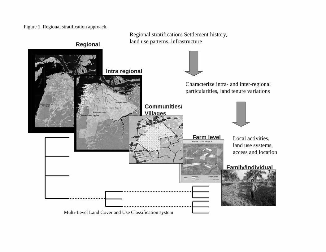
Figure 1. Regional stratification approach.

55°0'0"W

54°45'0"W

54°45'0"W

54°30'0"W

54°30'0"W

3°0'

0"S

3°0

'0"S

2°4

5'0

"S

2°4

5'0

"S

2°3

0'0

"S

2°3

0'0

"S

2°15'0

"S

2°15'0

"S

Santarém

Rio

Tap

ajós

Rio Amazonas

Rio Curuá - UnaFloresta Nacional Do Tapajós

10 0 105 Kilometers

Curua Una - Region 1

Mujui dos Campos - Region 2

Moju-Jabuti - Region 3

Cuiaba-Santarem - Region4

Regional

Intra regional

Farm level

Characterize intra- and inter-regional particularities, land tenure variations

Local activities, land use systems, access and location

Regional stratification: Settlement history, land use patterns, infrastructure

Communities/Villages

Family/Individual

Multi-Level Land Cover and Use Classification system

Figure 2. Steps in image/data search and research design. 1. Define study area name and location (e.g., use UTM coordinates X and Y):

Latitude: from _____________ to _______________ Longitude: from _____________ to _______________

1.2 Find, select, and bookmark area using Google Earth, with overlays of roads, rivers, administrative maps and other relevant layers. Observe the regional topography and land cover, with particular attention to settlement patterns vis-à-vis land use and land cover. 1.3 Landsat WRS grid location:

WRS 1 (Landsat 1, 2, 3) Path____/Row____ WRS 2 (Landsat 4, 5) Path____/Row____ Quadrant (if applicable):_______________ Data quality (e.g., cloud cover)

1.4 Identify other data/sensors:

Sensor (airflight mission, satellite and sensor) Data type (analogic or digital) Format (if applicable)

2. Define a time-line of relevant events

3. Characterize seasonality and vegetation phenology

4. Graph or cross-tabulate ‘IDEAL’ sampling and IDENTIFIED available remote sensing data and maps in the context of each research question

Temporal resolution and data (e.g. bi-yearly, Spring and Fall) Spatial resolution and data (e.g., Landsat TM, Path 20/Row 47)

5. Decide on data selection, refine/revise research questions according to available data (temporal sampling) and data resolution (spatial). Consider data temporal availability and spatial resolution to land use and cover spatial-temporal patterns, and define minimum mapping units and processing needs.

Climate Land cover Land use

Temporal

Spat

ial

Historical events Socio-Economic change Natural events Others…

Temporal (yearly to decadal)

Spat

ial

Figure 3. A general training guide for social scientists developing expertise in RS & GIS

Elements of RS Physical Principles Light Atmosphere Surface Sensor Inventory use sin the Anthropology Initial software training

Data structure Spectral Spatial Radiometric Temporal Sensor types & characteristics Searching tools Research questions and sensors

Geometric correction Image registration Principles of Radiometric & atmospheric correction Principles of band transformation Image subsetting

Interaction of spectral bands and surface elements Single band interpretation Color composite Data transformation

Principles of classification systems Classification algorithms functioning Unsupervised classification Training samples and field data Hybrid classification Principles of visual interpretation

Classification accuracy assessment Change detection methods Transition matrix Digital and analogic comparison Products, results and map preparation

Basic Principles Elements of GIS Types of software

Basic map manipulation and importing tools Data structure Cartographic projections and conversions

Cross-tabulation Field products, maps Modeling interfaces Network analysis

Change detection routines Accuracy assessment Products

Rem

ote se

nsin

g G

IS

Introduction to principles Becoming familiar with data Pre-processing, Classification Change detection, and social science manipulation & developing and applications accuracy assessment, applications research questions products