bryce cooke miguel robles - international food policy research

IFPRI Discussion Paper No. 00942

December 2009

Recent Food Prices Movements

A Time Series Analysis

Bryce Cooke

Miguel Robles

Markets, Trade and Institutions Division

INTERNATIONAL FOOD POLICY RESEARCH INSTITUTE

The International Food Policy Research Institute (IFPRI) was established in 1975. IFPRI is one of 15 agricultural research centers that receive principal funding from governments, private foundations, and international and regional organizations, most of which are members of the Consultative Group on International Agricultural Research (CGIAR).

FINANCIAL CONTRIBUTORS AND PARTNERS IFPRI’s research, capacity strengthening, and communications work is made possible by its financial contributors and partners. IFPRI receives its principal funding from governments, private foundations, and international and regional organizations, most of which are members of the Consultative Group on International Agricultural Research (CGIAR). IFPRI gratefully acknowledges the generous unrestricted funding from Australia, Canada, China, Finland, France, Germany, India, Ireland, Italy, Japan, Netherlands, Norway, South Africa, Sweden, Switzerland, United Kingdom, United States, and World Bank.

AUTHORS Bryce Cooke, George Washington University Ph.D. Student , Economics Department Email: [email protected] Miguel Robles, International Food Policy Research Institute Research Fellow, Markets, Trade and Institutions Division Email: [email protected]

Notices 1 Effective January 2007, the Discussion Paper series within each division and the Director General’s Office of IFPRI were merged into one IFPRI–wide Discussion Paper series. The new series begins with number 00689, reflecting the prior publication of 688 discussion papers within the dispersed series. The earlier series are available on IFPRI’s website at http://www.ifpri.org/category/publication-type/discussion-papers. 2 IFPRI Discussion Papers contain preliminary material and research results, and have been peer reviewed by at least two reviewers—internal and/or external. They are circulated in order to stimulate discussion and critical comment.

Copyright 2009 International Food Policy Research Institute. All rights reserved. Sections of this document may be reproduced for noncommercial and not-for-profit purposes without the express written permission of, but with acknowledgment to, the International Food Policy Research Institute. For permission to republish, contact [email protected].

mailto:[email protected]�


http://www.ifpri.org/category/publication-type/discussion-papers�


iii

Contents

Acknowledgments v

Abstract vi

1. Introduction 1

2. Data 3

3. Econometric Modeling 16

4. Concluding Remarks 30

Appendix 32

References 34

iv

List of Tables

1. Explanations for rise in agricultural commodity prices 2 2. Data and variables 3 3. Unit root tests (ADF) 17 5. Corn price: First differences econometric analysis 19 6. Wheat price: First differences regressions 21 7. Soybean price: First differences regressions 22 8. Rice price: First difference regression 24

List of Figures

1. Monthly corn price (US no. 2 yellow corn at Gulf of Mexico) 4 2. Monthly wheat price (US no. 2 hard red winter at Gulf of Mexico) 5 3. Monthly soybean price (US no.1 yellow soybean at Gulf of Mexico) 5 4. Monthly rice price (Thai A1 broken white rice, F.O.B. Bangkok) 6 5. Monthly oil prices (Cushing, OK WTI) 6 6. U.S. ethanol production 7 7. U.S. biodiesel production 8 8. Fertilizer prices 8 9. Exchange rates 9 10. Real world demand 10 11. World commodity exports 11 12. Futures contracts: Monthly traded volumes (3 months moving average, 1st quarter 2002=100) 12 13. Futures contracts: Monthly open interest (3 months moving average, 1st quarter 2002=100) 13 14. Futures contracts: Ratio volume to open interest (Monthly volume / monthly open interest) 14 15. Futures contracts: Importance of noncommercial positions 14 16. Wheat exports Granger-cause wheat prices 25 17. Exchange rates Granger-cause rice prices 26 18. World demand Granger-causes rice prices 26 19. Soybean exports Granger-cause soybean prices 27 20. Oil prices Granger-cause soybean prices 27 21. Oil prices Granger-cause corn prices 28 22. Granger causality: Speculation proxies 29 A.1. Chow tests (top: one-step, bottom: breakpoint) on whole set of full corn differencing equation 32 A.2. Chow tests (top: one-step, bottom: breakpoint) on shortened set of full corn differencing

equation 32 A.3. Chow tests (op: one-step, bottom: breakpoint) on whole set of wheat with noncommercial long

ratio speculation differencing equation 33 A.4. Chow tests (top: one-step, bottom: breakpoint) on whole set of wheat with noncommercial long

ratio speculation differencing equation 33

v

ACKNOWLEDGMENTS

We would to thank Kyosti Pietola and Maximo Torero for their comments and suggestions and the anonymous referee who also provided comments on an earlier version of this paper. Excellent research assistance has been provided by Pablo Flores who updated the data and econometric analysis of a draft version of this paper including data only up to mid 2008. The usual disclaimer applies.

vi

ABSTRACT

From 2006 to mid-2008 the international prices of agricultural commodities increased considerably, by a factor larger than two. This upward trend in agricultural prices captured the world’s attention as a new food crisis was emerging. Several explanations for these movements in prices, ranging from demand-driven forces to supply shocks, have been provided by analysts, researchers, and development institutions. This paper is an attempt to empirically validate these explanations using time series econometrics and data at monthly frequency. We focus on the international price of corn, wheat, rice, and soybeans. First, we identify variables associated with the factors mentioned as causing the increase in these agricultural commodities prices. Second, we use time series analysis to try to quantitatively validate those explanations. The empirical work presented here includes first difference models and rolling Granger causality tests. Overall, our empirical analysis mainly provides evidence that financial activity in futures markets and proxies for speculation can help explain the observed change in food prices; any other explanation is not well supported by our time series analysis.

Keywords: food crisis, time series, speculation, agricultural commodity prices, granger causality

1

1. INTRODUCTION

From 2006 to mid-2008 the international price of agricultural commodities showed an upward trend of a magnitude not seen since the seventies. As a result, in mid-2008 the prices of wheat, corn, rice, and soybeans were more than two times the levels observed on 2006, and the situation led to a great deal of concern because high food prices may have devastating effects in the developing world in terms of increasing hunger and poverty. Several explanations have been given for the source of the newly observed upward trend in food prices. Some of them emphasize world demand factors, while other explanations accentuate supply-side changes. Here we summarize these explanations and in Table 1, we provide references where further elaboration on each explanation can be found.

There are at least four demand-driven explanations. First, there is the notion of a rising world demand for a variety of food products in BRIC (Brazil, Russia, India, and China) as well as other populous nations that have achieved great economic improvements in recent years. Also it is argued that in these countries, higher household incomes translate into growing meat consumption, which leads to an increasing demand for animal feed. Second, there is increasing production of ethanol and biofuels, as subsidies in the United States and Europe have pushed up the supply of these products, which in turn calls for larger demands of agricultural commodities as inputs. Third, there is increasing activity and speculation in futures markets of agricultural commodities. Some analysts note that there are no economic fundamentals that can capture the huge increase in prices, and therefore they point to a speculative bubble that will burst sooner or later. A fourth explanation is an easy monetary policy in the United States until 2007, which initially has been reflected in commodity prices, among them agricultural commodities, but will eventually translate into inflationary pressures. This would also explain a weakening dollar, and as long as prices are set in dollars, higher prices are needed to keep parities in other currencies.

Supply-side explanations range from low research and development (R&D) investments in agriculture over the recent years to higher key input prices of oil and fertilizers. Higher oil prices not only directly affect the supply of food as transportation costs rise but also make ethanol and biofuel production more profitable and hence exacerbate the demand for grains. Also, as a response to higher food prices, some countries have imposed trade barriers and export restrictions, tightening the world supply of food even further. Climate change and transitory weather-related supply shocks have also been part of the menu of explanations.

However, we are not aware of any study that has tried to validate empirically and quantify the relative importance of these different explanations when considering them simultaneously in explaining the short- and medium-run dynamics of agricultural prices. In this paper we look for the empirical support (or lack of support) of these explanations. Hence, we conduct a time series analysis, with high-frequency data (monthly), to better understand the dynamics of agricultural commodities prices and the incidence of different explanations in their dynamics. Because we use monthly data, we are able to capture short-term shocks that might have affected the international agricultural commodity markets. In particular we focus on four agricultural commodities: corn, wheat, rice, and soybeans.

The remainder of the paper is organized as follows. In Section 2 we describe the data collected and how the selected variables are linked to different explanations of the increase in agricultural commodities prices. In Section 3 we present the results of our time series modeling analysis. First, we study the properties of each individual series to assess the presence of unit roots. Next, we model the price of each agricultural commodity (wheat, maize, rice, soybeans) in a pure first-differences fashion. Finally we conduct rolling granger causality tests of every exogenous variable on each of the four commodity prices. We also provide comments on our attempt to use a vector error correction model approach and single equations error correction modeling. Concluding remarks are given in Section 4.

2

Table 1. Explanations for rise in agricultural commodity prices

Factors Mechanism References Demand-side factors Rising world demand Emerging nations can afford more

diversified food consumption basket. Increased demand as direct consumption as well as animal feed.

Abbott et. al. 2008, FAO 2000b, Mitchell 2008, OECD 2008, Trostle 2008, Von Braun 2007, World Bank 2008

Ethanol/biofuels Greatly increased use for limited good. Abbott et. al. 2008, FAO 2000b, Mitchell 2008, OECD 2008, Trostle 2008, Von Braun 2007, World Bank 2008

Increased activity in futures market

Larger percentage of marketplace has no intent of taking futures to delivery, increasing short-run price volatility

Abbott et. al. 2008, Irwin 2008, Masters 2008, Mitchell 2008,

Supply-side factors Increased oil/fertilizer prices Higher costs to food producers limit

production. Abbott et. al. 2008, FAO 2000b, Mitchell 2008, OECD 2008, Trostle 2008, Von Braun 2007, World Bank 2008

Low R&D investments in agriculture

Less research on how to increase yield has limited production growth.

Abbott et. al. 2008, FAO 2000b, Mitchell 2008, OECD 2008, Trostle 2008, Von Braun 2007, World Bank 2008

Trade barriers/ export restrictions

Creating greater scarcity worldwide increases commodity prices.

Abbott et. al. 2008, FAO 2000b, Mitchell 2008, OECD 2008, Trostle 2008, World Bank 2008

Droughts Occurring in large grain-producing nations lowers worldwide production.

Abbott et. al. 2008, FAO 2000b, Mitchell 2008, OECD 2008, Trostle 2008, Von Braun 2007, World Bank 2008, von Braun 2007

Other factors Dollar devaluation Most commodities’ indicator prices are

quoted in U.S. dollars. Abbott et. al. 2008, Mitchell 2008, Von Braun 2007

3

2. DATA

In this section we describe the data collected and used in our time series modeling of the agricultural commodities prices. Other than prices, our data includes variables reflecting demand and supply factors affecting agricultural prices. All our series are on a monthly basis. On the demand side we consider a monetary aggregate (real M2) as a proxy for world real aggregate expenditure, production of ethanol and biodiesel, several proxies for trading activity in futures markets, and the U.S. dollar–Euro exchange rate. On the supply side we consider the price of oil, price of fertilizers, and volume of exports by major world producers. Table 2 summarizes the data collected.

Table 2. Data and variables

Var iable Descr iption Source Corn Price Monthly average price in US$/ton of US yellow no.

2 corn at the Gulf of Mexico FAO International Commodity Price Database

Wheat Price Monthly average price in US$/ton of US no. 2 hard red winter wheat at the Gulf of Mexico

FAO International Commodity Price Database

Soybean Price Monthly average price in US$/ton of US no. 1 yellow soybean at the Gulf of Mexico


Rice Price Monthly average price in US$/ton of Thai A1 white broken rice at Bangkok


Oil Price US dollars per barrel at Cushing, OK Energy Information Administration Ethanol Production Millions of gallons produced each month in the US Energy Information Administration Biodiesel Production Millions of gallons produced each month in the US Energy Information Administration Fertilizer Prices US$/MT data of five major fertilizers, as well as an

index USDA & World Bank Commodity Price Database

Exchange Rate US$/euro exchange rate Federal Reserve Bank of St. Louis Economic Database

Worldwide Real M2 A proxy for world demand, it is a weighted index of the largest economies’ real M2

IMF’s IFS Database

Grains Exports A proxy for world supply, it combines top exporters’ figures for each grain market separately

US Census Bureau’s Foreign Trade Division, Eurostat Comex, AliceWeb, CanSim, Bank of Thailand, Argentina Secretary of Agriculture

Volume Total number of trading on a commodity futures contract

Chicago Board of Trade (CBOT)

Open Interest Number of futures that have not yet been offset by an opposite futures nor fulfilled by delivery of the commodity exercise

CBOT

Volume to Open Interest Ratio

Captures speculation assuming majority of speculators prefer to get in and out of the market on a short period of time

CBOT

Noncommercial to Total Trade Ratio (long and short positions)

Noncommercial positions in futures contracts mainly represent speculative activity in search for financial profits

U.S. Commodity Futures Trading Commission

4

As we mentioned all data collected were monthly, and the time period was from 2002 to early 2009, depending upon the commodity price under analysis. The end of the series was restricted due to unavailable data, and restrictions at the beginning of the series were due to the presence of structural changes based on Chow tests, which are described in Section 3. All price data and other variables will be taken in log form when analyzed.

The pricing data for the agricultural commodities was retrieved from the FAO International Commodity Prices Database. The corn product considered was U.S. yellow no. 2 maize, and the others were soft wheat, Thai rice A1, and soybeans (as opposed to meal or oil). All series are denoted in dollars per metric ton ($/MT).

As can be seen in Figure 1, the price of corn has more than doubled between the fourth quarter of 2006 and the second quarter of 2008. Before 2006 the average monthly growth rate was 0.2%, and since then the monthly growth rate jumped to 3.9% in 2006. Though it slowed to 0.8% in 2007, it was 6.4% in the first half of 2008. By the first half of 2009 the growth rate of corn prices went back to a rather normal level, 0.92%. Also the coefficient of variation (standard deviation divided by mean) has increased over time, showing evidence of an increase of volatility as well. For the period 2002–2005 this coefficient is 0.10, and between 2006 and 2009 is 0.16.

Figure 1. Monthly corn price (US no. 2 yellow corn at Gulf of Mexico)

Source: FAO International Commodity Prices Data Base

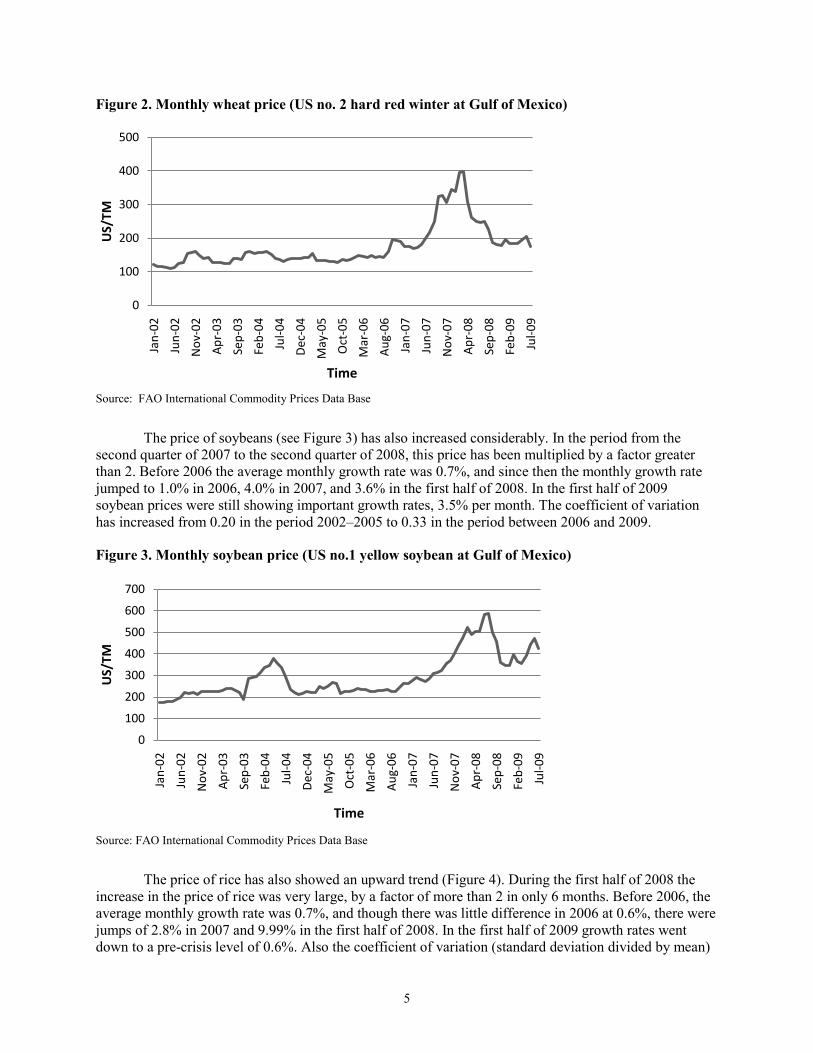
In Figure 2 we show the recent evolution of wheat price. It has also more than doubled between the first quarter of 2006 and the second quarter of 2008. Before 2006, the average monthly growth rate was 0.56%, and since then the monthly growth rate jumped to 2.10% in 2006 and 5.10% in 2007; but then in the first half of 2008, prices actually decreased by 0.87% per month on average. In 2009 also prices increased less than the high growth rates of 2007 and first months of 2008 (2.8% per month). Also the coefficient of variation has increased over time. For the period 2002–2005 this coefficient is 0.11, and between 2006 and 2009 is 0.25.8 and in 2009.

0

100

200

300

400

Jan-

02

Jul-0

2

Jan-

03

Jul-0

3

Jan-

04

Jul-0

4

Jan-

05

Jul-0

5

Jan-

06

Jul-0

6

Jan-

07

Jul-0

7

Jan-

08

Jul-0

8

Jan-

09

Jul-0

9

US/

TM

Time

5

Figure 2. Monthly wheat price (US no. 2 hard red winter at Gulf of Mexico)


The price of soybeans (see Figure 3) has also increased considerably. In the period from the second quarter of 2007 to the second quarter of 2008, this price has been multiplied by a factor greater than 2. Before 2006 the average monthly growth rate was 0.7%, and since then the monthly growth rate jumped to 1.0% in 2006, 4.0% in 2007, and 3.6% in the first half of 2008. In the first half of 2009 soybean prices were still showing important growth rates, 3.5% per month. The coefficient of variation has increased from 0.20 in the period 2002–2005 to 0.33 in the period between 2006 and 2009.

Figure 3. Monthly soybean price (US no.1 yellow soybean at Gulf of Mexico)


The price of rice has also showed an upward trend (Figure 4). During the first half of 2008 the increase in the price of rice was very large, by a factor of more than 2 in only 6 months. Before 2006, the average monthly growth rate was 0.7%, and though there was little difference in 2006 at 0.6%, there were jumps of 2.8% in 2007 and 9.99% in the first half of 2008. In the first half of 2009 growth rates went down to a pre-crisis level of 0.6%. Also the coefficient of variation (standard deviation divided by mean)

0

100

200

300

400

500Ja

n-02

Jun-

02

Nov

-02

Apr

-03

Sep-

03

Feb-

04

Jul-0

4

Dec

-04

May

-05

Oct

-05

Mar

-06

Aug

-06

Jan-

07

Jun-

07

Nov

-07

Apr

-08

Sep-

08

Feb-

09

Jul-0

9

US/

TM

Time

0

100

200

300

400

500

600

700

Jan-

02

Jun-

02

Nov

-02

Apr

-03

Sep-

03

Feb-

04

Jul-0

4

Dec

-04

May

-05

Oct

-05

Mar

-06

Aug

-06

Jan-

07

Jun-

07

Nov

-07

Apr

-08

Sep-

08

Feb-

09

Jul-0

9

US/

TM

Time

6

has increased over time, showing evidence of an increase of volatility as well. For the period 2002–2005 this coefficient is 0.18, and between 2006 and 2009 is 0.4874.

Figure 4. Monthly rice price (Thai A1 broken white rice, F.O.B. Bangkok)


Monthly data on oil prices was retrieved from the Energy Information Administration, and prices are in U.S. dollars per barrel (see Figure 5). Starting in 2003 until the first quarter of 2008 the price of oil showed an upward trend that originated a major concern worldwide and put the world in an oil crisis situation. However by the fourth quarter of 2008 oil prices quickly decreased and went down to 2004 levels. In the first half of 2009 oil prices again increased but far from reaching the peak levels of the beginning of 2008. It is important to notice that while the strong upward trend in oil prices dates back to 2003, the rise in food prices was not observed any earlier than 2006.

Figure 5. Monthly oil prices (Cushing, OK WTI)

Source: Energy Information Administration

0100200300400500600700800900

Jan-

02

Jun-

02

Nov

-02

Apr

-03

Sep-

03

Feb-

04

Jul-0

4

Dec

-04

May

-05

Oct

-05

Mar

-06

Aug

-06

Jan-

07

Jun-

07

Nov

-07

Apr

-08

Sep-

08

Feb-

09

Jul-0

9

US/

TM

Time

020406080

100120140160

Jan-

02

Jun-

02

Nov

-02

Apr

-03

Sep-

03

Feb-

04

Jul-0

4

Dec

-04

May

-05

Oct

-05

Mar

-06

Aug

-06

Jan-

07

Jun-

07

Nov

-07

Apr

-08

Sep-

08

Feb-

09

Jul-0

9

US$

Bar

ril

Time

7

Also, ethanol production in the United States is denoted in millions of gallons (see Figure 6). This data can be found in the Energy Information Administration’s Monthly Energy Review. Ethanol production in the United States has increased considerably since 2003 due in part to government assistance and subsidies. As a result, the ethanol industry in the United States has become an important source of corn demand; however, its contribution as an alternative source of fuel is relatively small. In 2006–2007, 20.1% of corn production was supplied to the ethanol industry, and this number is estimated to reach 24.2% in 2009–2010.1 In the gasoline market fuel ethanol production in the United States explained only 5.6% of total motor gasoline consumption in 2008.2

Figure 6. U.S. ethanol production

It is estimated that the conversion rate of corn is at 2.7 gallons per bushel.

U.S. biodiesel production (see Figure 7) data can be found at EIA’s Monthly Energy Review, also taken in millions of gallons. The United States is the second largest producer, but produces only a quarter that of its European counterpart. Obviously, European data would have been preferred, but attempts at finding monthly data were unsuccessful. However, Europe uses more rapeseed and sunflower in their production than soybean, whereas the soybean is the main agricultural product used in the United States. Also in the United States, biodiesel production is relatively less important as it amounts to only 10% of ethanol output. In terms of its importance in demanding agricultural commodities, it is estimated that in 2008 U.S. biodiesel industry demanded less than 1.2% of total U.S. soybean production.

For the price of fertilizers we use the fertilizer price index provided by the USDA as well as price series for potassium chloride, urea, DAP, phosphate rock, and TSP, which were made available by the World Bank Commodity Price Database (see Figure 8).

1 Own estimates based on information provided by World Agricultural Supply and Demand Estimates, WASDE - 475,

October 2009, USDA. 2 Own estimates based on information from the Annual Energy Review 2008, Energy Information Administration.

0100200300400500600700800900

1000

Jan-

02

Jun-

02

Nov

-02

Apr

-03

Sep-

03

Feb-

04

Jul-0

4

Dec

-04

May

-05

Oct

-05

Mar

-06

Aug

-06

Jan-

07

Jun-

07

Nov

-07

Apr

-08

Sep-

08

Feb-

09

Jul-0

9

Mill

ons

of G

allo

ns P

rodu

ced

Time

8

Figure 7. U.S. biodiesel production

Source: Energy Information Administration

Figure 8. Fertilizer prices

Source: World Bank Commodities Price Database, USDA

Also, we consider exchange rates to analyze if the dollar depreciation can explain price movements. The U.S. dollar–euro exchange rate was chosen, and it is denoted in the number of dollars necessary to buy one euro; hence, a positive change implies a depreciation of the dollar against the euro. As can be seen in the graph below, the dollar has been depreciating since 2002, with an accumulated loss of more than 65%. This data is found at the Federal Reserve Branch of St. Louis database.

0102030405060708090

Jan-

02

Jun-

02

Nov

-02

Apr

-03

Sep-

03

Feb-

04

Jul-0

4

Dec

-04

May

-05

Oct

-05

Mar

-06

Aug

-06

Jan-

07

Jun-

07

Nov

-07

Apr

-08

Sep-

08

Feb-

09

Jul-0

9

Mill

ons

of G

allo

ns P

rodu

ced

Time

0

200

400

600

800

1000

1200

1400

Jan-

02

Jun-

02

Nov

-02

Apr

-03

Sep-

03

Feb-

04

Jul-0

4

Dec

-04

May

-05

Oct

-05

Mar

-06

Aug

-06

Jan-

07

Jun-

07

Nov

-07

Apr

-08

Sep-

08

Feb-

09

US$

/TM

Fertilizer DAP Phosphate Potchloride TSP Urea

9

Figure 9. Exchange rates

Source: Federal Reserve Branch of St. Louis database

In order to create a proxy for world demand or aggregate expenditure, a real M2 worldwide index was constructed using individual M2 series for the 12 countries with the largest GDP (accounting for over 85% of world GDP) including the euro area, the United States, BRIC, as well as other large economies like other G8 nations (see Figure 10). Data on M2 was available at the IMF’s International Financial Statistics (IFS) database, and this was divided by each country’s CPI, also found at the IFS Database. Then, each real M2 index (January 2002 = 100) was used to construct a weighted index based on the size of the country’s GDP in U.S. dollars adjusted by purchasing power parity (PPP). We notice that four of the fastest growing M2 countries are Brazil, Russia, India and China, and hence the ones supporting a strong worldwide demand.

In order to capture shocks to the world supply of commodities, we choose to look at export data for the largest exporters. This supply proxy was chosen because other variables, such as production and yields, are not available at a monthly frequency. Also, looking at exports allowed us to capture a shortage in the world supply as several commodity producer countries have imposed restrictions to their exports (such as Argentina, Vietnam, India). In the corn market, data for the United States, European Union, and Argentina is collected, which accounted for 80% of exports in 2002. In the wheat market, data for the United States, European Union, Canada, and Argentina make up nearly three-quarters of the worldwide 2002 export market. With the United States, Brazil, and Argentina, 90 percent of the worldwide soybean market is considered, and Thailand data on rice exports can account for over half of world trade in that commodity.

All U.S. data was made available by the U.S. Census Bureau’s Foreign Trade Divisions available online at www.usatradeonline.gov. EU data can be found at Eurostat Comext; Brazil’s export data is available at AliceWeb; and Canada’s wheat data can be found at CanSim, all available online. Thailand data comes from the Bank of Thailand, and Argentina’s information can be found online at the Argentinian Secretary of Agriculture website. By looking at exports, a government’s policy actions taken to restrict agricultural trade will also be captured in explaining further price increases.

Also, a variety of proxies for participation in agricultutal commodity futures markets and speculative activity were chosen: (1) volume in futures contracts, (2) open interest in futures contracts, (3) the ratio of volume to open interest in futures contracts, and (4) positions in futures contracts by noncommercial traders.

0

0.4

0.8

1.2

1.6

2Ja

n-02

Jun-

02

Nov

-02

Apr

-03

Sep-

03

Feb-

04

Jul-0

4

Dec

-04

May

-05

Oct

-05

Mar

-06

Aug

-06

Jan-

07

Jun-

07

Nov

-07

Apr

-08

Sep-

08

Feb-

09

Jul-0

9

US

$ pe

r Eu

ro

Time

10

Figure 10. Real world demand

Source: IMF International Finance Statistics

In order to capture shocks to the world supply of commodities, we choose to look at export data for the largest exporters. This supply proxy was chosen because other variables, such as production and yields, are not available at a monthly frequency. Also, looking at exports allowed us to capture a shortage in the world supply as several commodity producer countries have imposed restrictions to their exports (such as Argentina, Vietnam, India). In the corn market, data for the United States, European Union, and Argentina is collected, which accounted for 80% of exports in 2002. In the wheat market, data for the United States, European Union, Canada, and Argentina make up nearly three-quarters of the worldwide 2002 export market. With the United States, Brazil, and Argentina, 90 percent of the worldwide soybean market is considered, and Thailand data on rice exports can account for over half of world trade in that commodity.

All U.S. data was made available by the U.S. Census Bureau’s Foreign Trade Divisions available online at www.usatradeonline.gov. EU data can be found at Eurostat Comext; Brazil’s export data is available at AliceWeb; and Canada’s wheat data can be found at CanSim, all available online. Thailand data comes from the Bank of Thailand, and Argentina’s information can be found online at the Argentinian Secretary of Agriculture website. By looking at exports, a government’s policy actions taken to restrict agricultural trade will also be captured in explaining further price increases.

Also, a variety of proxies for participation in agricultutal commodity futures markets and speculative activity were chosen: (1) volume in futures contracts, (2) open interest in futures contracts, (3) the ratio of volume to open interest in futures contracts, and (4) positions in futures contracts by noncommercial traders.

0

20

40

60

80

100

120

140

160

180

Jan-

02

Jun-

02

Nov

-02

Apr

-03

Sep-

03

Feb-

04

Jul-0

4

Dec

-04

May

-05

Oct

-05

Mar

-06

Aug

-06

Jan-

07

Jun-

07

Nov

-07

Apr

-08

Sep-

08

Feb-

09

Jul-0

9

US

$ N

orm

aliz

ed W

orld

M2p

er E

uro

Time

11

Figure 11. World commodity exports

Source: U.S. Census Bureau's Foreign Trade Eurostat Comext, AliceWeb, CanSim

Monthly volume in futures contracts.-This indicator captures the total number of trading on a commodity futures contract in the Chicago Board of Trade (CBOT) on a monthly basis. Also this indicator aggregates over contracts with different maturities. Note that typically contracts with maturities within the range of 24 months or more are traded. As shown in Figure 12, in recent years traded volumes in futures of agricultural commodities have increased vigorously. In 2006 the average monthly volume in futures for wheat and corn grew by more than 60% with respect to the previous year, and for rice, 40%. Also volumes in 2007 went up significantly for all four commodities, especially for soybeans, with a monthly average 40% larger than in 2006. During the first five months of 2008 only the volumes for corn seem to have stabilized, while the volumes for rice and soybeans were still growing at very high rates, 47% and 40%, respectively. Nevertheless, from mid 2008 to the first quarter of 2009 the average monthly volume in futures for all four commodities decreased, especially for rice (with 7%). Several reasons might explain the observed increase in volumes over recent years (until 2008), one of them being a more active participation of speculators in these markets, especially the participation of short-term speculators. Those opening and closing positions in a relative short period of time could have been a source of soaring volumes and subsequent impact on prices.

01,000,0002,000,0003,000,0004,000,0005,000,0006,000,0007,000,0008,000,0009,000,000

10,000,000

Jan-

02

Jun-

02

Nov

-02

Apr

-03

Sep-

03

Feb-

04

Jul-0

4

Dec

-04

May

-05

Oct

-05

Mar

-06

Aug

-06

Jan-

07

Jun-

07

Nov

-07

Apr

-08

Sep-

08

Feb-

09

MT

riceexp cornexp soyexp wheatexp

12

Figure 12. Futures contracts: Monthly traded volumes (3 months moving average, 1st quarter 2002=100)

Monthly open interest in futures contracts -This variable describes the total number of futures contracts of a given commodity that have not yet been offset by an opposite futures nor fulfilled by delivery of the commodity exercise. Every time a trader takes a position in the futures market (either long or short), immediately an open position is generated until this trader takes the opposite position or the contract reaches the expiration day. Open interest has also been growing over the past five years, as can be seen in Figure 13; however, for each commodity the average growth rates show important variations over time. In 2006, the average monthly open interest in futures for wheat and corn grew by about 75% with respect to the previous year, and for rice this number is larger than 90%. However, in 2007, the open interest slightly declined in corn and wheat, and there was moderate growth in rice at 21% growth. Soybeans, meanwhile, increased by 40% on average in 2007, but in 2008 the growth rate went down by 12% and in 2009 it recovered its positive path to about 8%. Furthermore, wheat experienced further decline in 2008, and corn was growing at a rate of only 3%. Our claim is that looking at open interest series may help us capture incoming medium- and long-term speculators in the commodity futures markets that may have played a role in the recent food prices crisis.

0

100

200

300

400

500

600

700Ja

n-02

Jun-

02

Nov

-02

Apr

-03

Sep-

03

Feb-

04

Jul-0

4

Dec

-04

May

-05

Oct

-05

Mar

-06

Aug

-06

Jan-

07

Jun-

07

Nov

-07

Apr

-08

Sep-

08

Feb-

09

Vol

ume

Inde

x

Corn Volume Wheat VolumeRice Volume Soybean Volume

Source: Chicago Board of Trade CBOT

13

Figure 13. Futures contracts: Monthly open interest (3 months moving average, 1st quarter 2002=100)

Ratio volume to open interest in futures contracts. We use this ratio to capture speculative market activity under the assumption that the majority of speculators prefer to get in and out of the market on a short period of time (see CBOT 2008c). Hence, a speculator taking opposite positions (buying and selling contracts) in the market within days or weeks will generate an increase in monthly registered volumes, but not much of a change on monthly open interest. Therefore, changes on this ratio would potentially capture changes in speculative activity. Empirically what we observe is that this ratio has shown little growth over the past few years; for instance, in 2006, the ratio was declining across all four commodities. In 2007, the results were mixed, with 31% growth in the wheat ratio and 17% in that for corn, but declining ratios for soybean and rice. In 2008, both corn and rice ratios were increasing, at 27% and 19% respectively, as wheat ratios continued to grow at 19% and corn declined slightly. Comparing this recent growth with 2005 and 2006, where at least three commodities’ ratios were declining on average, leads us to claim of the capacity of this ratio as a potential instrument to capture speculative behavior.

0

100

200

300

400

500

Jan-

02

Jun-

02

Nov

-02

Apr

-03

Sep-

03

Feb-

04

Jul-0

4

Dec

-04

May

-05

Oct

-05

Mar

-06

Aug

-06

Jan-

07

Jun-

07

Nov

-07

Apr

-08

Sep-

08

Feb-

09

Vol

ume

Inde

x

Wheat Open Interest Corn Open InterestRice Open Interest Soybean Open Interest


14

Figure 14. Futures contracts: Ratio volume to open interest (Monthly volume / monthly open interest)

Figure 15. Futures contracts: Importance of noncommercial positions

0

2

4

6

8

10

12Ja

n-02

Jun-

02

Nov

-02

Apr

-03

Sep-

03

Feb-

04

Jul-0

4

Dec

-04

May

-05

Oct

-05

Mar

-06

Aug

-06

Jan-

07

Jun-

07

Nov

-07

Apr

-08

Sep-

08

Feb-

09

Vol

ume

Inde

x

Wheat Volume Open Interest Corn Volume Open InterestSoybean Volume Open Interest Rice Volume Open Interest


0

0.2

0.4

0.6

0.8

1

Jan-

02

Jun-

02

Nov

-02

Apr

-03

Sep-

03

Feb-

04

Jul-0

4

Dec

-04

May

-05

Oct

-05

Mar

-06

Aug

-06

Jan-

07

Jun-

07

Nov

-07

Apr

-08

Sep-

08

Feb-

09

Rati

o

Weath nlong Corn nlong Rice nlong Soybean nlong


15

Importance of noncommercial positions in futures contracts. All reportable3 traders’ futures positions are classified by the Commodity Futures Trading Commission (CFTC) as either commercial or noncommercial. Futures positions in a commodity are classified as commercial if a trader uses futures contracts in that particular commodity for hedging purposes as defined by the CFTC; otherwise, a position will be classified as noncommercial. Hence, while commercial positions are held for hedging purposes, noncommercial positions in futures contracts mainly represent speculative activity in search for financial profits. We use this classification by the CFTC to study the importance of speculative activity relative to hedging activity over recent years. For this purpose we look at the ratio of noncommercial positions to total positions,4

The ratio of long noncommercial positions to total (long) positions seems to be growing in recent years. Between 2006 and 2008 there has been growth in the weekly average of the ratio in at least three of the four commodities markets. For corn this ratio was on average 0.29 in 2005, and in the first five months of 2008 it reached an average of 0.49. In 2009 this average decreased to 0.40. Similar increases have been observed for wheat and soybeans. In the case of rough rice this ratio has been more erratic over time; and although the ratio increased during 2009 compared with the previous year, the 2009 level was still lower than observed levels in past years. In the case of short positions there is less evidence of an upward trend of the relative importance of speculative positions in recent years. On the contrary, it seems that commercial short positions have become relatively more important. Overall it is apparent that an increasing participation by commercial hedgers in the futures markets has been matched by an increasing participation by speculative investors (or noncommercial ones). However, this does not mean that short positions by speculators may not have an effect on prices, because ultimately the volume of short positions by speculators, as well as by hedgers, has also strongly increased over time.

and we do this for long as well as for short positions.

Our one interpretation of the link between speculation and prices is the following. Typically in agricultural futures markets, producers are the ones selling short because they are looking to hedge their futures incomes, while industrial food processors take long positions, looking to hedge their costs. The volume of these two opposite positions does not necessarily coincide, and hence noncommercial traders play an important role in closing that gap and providing liquidity to the market. However, when participation of noncommercial players and speculators increases significantly on both sides of the market, then we argue that speculation has a more active role in driving prices. As a group of speculators enters the market taking long positions betting on higher future spot prices, futures prices might be driven upward to the point of attracting more conservative (with respect to their expectations about future spot prices) noncommercial traders.5

As this happens in futures markets, signals of higher prices are transmitted to the spot market in such a way that initial expectations are confirmed and provide feedback on further expectations. However, in this simplified example it’s not clear what triggers the initial higher participation of speculators. The point here is that this is one way in which one can rationalize the fact of increasing volume and participation by noncommercial traders and/or speculators and higher prices. Our approach is to construct proxies for speculation (certainly imperfect ones) and leave to the data tell us if those proxies have any explanatory power over spot prices.

3 Reportable traders are those who hold positions in futures and options at or above specific reporting levels set by the

Commodity Futures Trading Commission (CFTC). It is estimated that the aggregate of all traders’ positions reported accounts for more than 70% of the total open interest in any given market.

4 We use total reportable positions, because only reportable positions are classified as either commercial or noncommercial. 5 Masters (2008) argues that in recent years index funds have entered aggressively into commodity futures markets and that

they have contributed heavily to the food price inflation. Also he points out that typically these funds buy futures and then roll their positions by buying calendar spreads. In this case index funds would have contributed to the observed increased volume in futures contracts, not only on the buying side but also on the selling side of the market.

16

3. ECONOMETRIC MODELING

In this section we present the results of our time series modeling analysis. First, we study the properties of each individual series to assess the presence of unit roots, and we follow the standard practice in time series econometrics to use first differences if unit roots are found. Next, we model the price of each agricultural commodity (wheat, maize, rice, soybeans) in a pure first-differences fashion. We utilize a general-to-specific modeling approach, which attempts to discover which theoretical view is appropriate, instead of using the econometric analysis to support existing theory. After starting with a general hypothesis about the important variables, the model is teased down by testing certain restrictions on the general model. Finally we conduct rolling granger causality tests of every exogenous variable on each of the four commodity prices.

It is worth mentioning that as part of our empirical analysis we also conducted a four-variable error correction model (ECM) as well as single equations error correction representations. The four-variable approach was disregarded and found it to be inappropriate. This is because a Johansen Trace Test on a VAR that includes only the four commodity prices finds that there is no co-movement between any of the price series for the time period starting in 2002. We also concluded that for the price of any of our four commodities—rice, soybeans, corn, and wheat—a one-equation ECM is not the most adequate to capture their dynamics over time and co-movements with other variables. In the case of soybean, rice and corn we found one co-integrating relationship between the corresponding price and the exogenous variables. However, when attempting to model long-run relationships we didn’t find mean reversion in the system. For wheat we found a co-integrating relationship. In the long run, wheat prices are positively linked with oil, M2, and volume traded in futures contracts; and negatively related to ethanol, exchange rate, fertilizer prices, and biodiesel production. These latter negative relationships seem at odds with economic reasoning. Also the most parsimonious short term model we found is one that considers only the error correction term and the noncommercial long position ratio. Hence some indication was found that fundamentals and volume of trading determine the long-run price, but a proxy for speculation in the futures market alone determines short-run movements in the spot price, even though this is not a rich short-term specification. An additional limitation in the case of wheat is that we cannot really claim a single-equation ECM as ethanol production and volume traded in futures contracts cannot be treated as exogenous variables6

Properties of the Individual Series

.

In order to test whether the series are I(1) (integrated of order 1) or have a unit root, augmented Dickey-Fuller (ADF) tests are used to analyze the variables (after taking logs). We remind the reader that the null hypothesis of the ADF test is the existence of a unit root. After checking over multiple time periods, January 1998 through December 2007 as well as January 2002 through December 2007, we find that the ADF tests fail to reject the null hypothesis for any number of lagged differences (see next paragraph) chosen for all the variables except for volume to open interest ratio (volume and open interest refer to futures contracts) as well as exports (see Table 3). Therefore, those series that fail to reject the null hypothesis are at least I(1) in this data set. Note that noncommercial ratios (long or short positions in futures contracts by noncommercial traders divided by total reportable positions) are by definition I(0), because their values are necessarily bounded between zero and one, and therefore are not tested here.

In this paragraph we clarify what is meant by the “number of lagged differences chosen.” For ADF tests, there are three important conditions that will help to define whether a series is stationary, or I(0), (though some series will be stationary or not regardless of these three factors). The first is the time period chosen. The time period chosen here will always begin in January 2002 and ends in June 2009 for variables in the corn, wheat, and rice equations; but it ends in December 2007 for the soybean equation

6 We do not include results of the four-price ECM and single equations ECM here given we disregarded those approaches. However the analysis is available upon request to the authors

17

due to data constraints. The second is whether to include a constant or a constant and trend when doing ADF tests. Here, only a constant is used because we don’t want to rely on a deterministic time trend.7

The last is defining the number of lagged differences chosen in an ADF test. To test if is I(1), use the next higher difference:

, where “n” is the number of lagged differences used. In principle for different numbers of lagged differences used, it is possible to find that the series may give conflicting opinions about whether the series is I(1). Here, all four equations that analyze prices based on past prices and exogenous variables are appropriate to analyze with two lags, as was specified by the Bayesian-Schwartz criterion (BSC), so ADF tests are performed accordingly.

Now, to test if the series are integrated of order 2, or I(2), we use the ADF test on the differences of the levels and logged data. Given the time periods considered here, we conclude that none of the series are I(2). Also, it was important to ensure that none of the series have seasonality. Even though the series do not appear to have seasonal trends on the data plots, each series was mapped into an AR(13) process to see if such an effect does exist. After viewing significance tests and using lag structure analysis, specifically the Akaike Information criterion (AIC), Wald tests, and BSC, we find that none of the series show any evidence of seasonality. We tested to see if the data could be better represented by ARMA processes than autoregressive modeling, and all three criterion (BSC, AIC, and Hannan-Quinn) suggest using AR processes.

Table 3. Unit root tests (ADF)

Var iables ADF t-

stat,*5% ,**1% Var iables ADF

t-stat,*5% ,**1%

L(Wheat Price) 0.5031 L(Corn Volume Open Interest) -2.3071 L(Corn Price) 0.0194 L(Soybean Volume Open Interest) -4.0788** L(Soybean Price) -1.0178 L(Rice Volume Open Interest) -2.815 L(Rice Price) 1.9024 L(Wheat Exports) -3.1064 L(Wheat Volume) -1.6754 L(Corn Exports) -3.4151* L(Corn Volume) -1.2201 L(Soybean Exports) -4.6533** L(Soybean Volume) -1.8619 L(Rice Exports) -2.6069 L(Rice Volume) -2.9211 L(Fertilizers) -1.0323 L(Wheat Open Interest) -1.1463 L(Oil) -1.9474 L(Corn Open Interest) -1.3783 L(Ethanol) -0.5243 L(Soybean Open Interest) -1.6406 L(Biodiesel) -0.9992 L(Rice Open Interest) -1.7239 L(M2) 1.9075 L(Wheat Volume Open Interest) -2.3311 L(Exchange Rate) -2.6721

Note: note: L(X) = log(X)

First Differences

We use turn here to first differencing models to explain all grains prices. A first differencing representation is given by:

7 One can hardly argue for a deterministic time trend because before the increase in prices over the last three years, prices have been declining for a long period of time.

18

In this representation transitory shocks in the growth rate of exogenous variables affect the dynamics of the growth rate of prices, and as long as the effects will vanish over time, in other words the model shows mean-reversion. In the case of a permanent shock to the growth rate of any exogenous variable then that will have a permanent effect in the equilibrium growth rate of prices

Corn Price

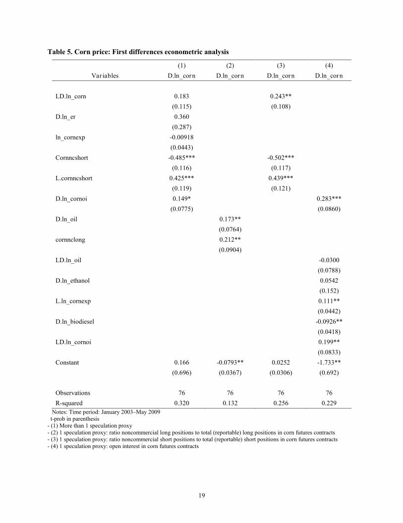
When analyzing corn prices, all other variables are strongly exogenous, according to Granger causality tests. Testing for the appropriate lag structure, using the BSC, we find that only one lag in differences is necessary. Notice that we have five speculation proxies available, some of which are highly correlated, and therefore we carefully look at different specifications using different speculation proxies. When first attempting this analysis for the entire series, the breakpoint Chow tests find that our most efficient models are not able to correctly describe the environment because the first few observations in the data set behave differently than the rest. For all regressions, analysis begins in January 2003 because of these Chow tests. Table 5 shows results for different model specifications8

What we find more interesting is that three speculation proxies show explanatory power in our regressions. The fraction of long positions in futures contracts by noncommercial traders, the fraction of short positions in futures contracts by noncommercial traders, and total open interest in corn futures contracts seem to partially explain corn price growth rate (notice that regressions 2 and 5 in Table are not autoregressive processes).

; in all cases we teased down the regressions such that only significant variables remain in the model. Overall, our regressions do not accomplish a high goodness of fit, which is not surprising considering we are modeling prices at monthly frequency. Also we find that very few variables have any explanatory power other than speculation proxies, and when they do, they do not necessarily enter with the sign one would have expected. This is the case for the dollar devaluation rate, which enters one regression with a negative sign; in another specification the growth rate of the oil price also shows a negative sign although with a 15 percent significance level. In one specification we find that the lagged growth rate of ethanol production positively affects the growth rate of corn prices, while the growth rate of oil prices enters with a negative sign. Indeed is not clear to us what effect this variable is picking. In this same regression, accelerations in the production of biodiesels have a negative effect; in this case we cannot think of a convincing economic interpretation. Also we must say that as we move across different specifications, we end up with different significant explanatory variables that indicate poor robustness in our econometric analysis.

8 In all specifications we test for the appropriate lag structure according to the BSC. When trying to use total volume in

futures contracts, the number of lags required leaves us with no degrees of freedom.

19

Table 5. Corn price: First differences econometric analysis

(1) (2) (3) (4) Var iables D.ln_corn D.ln_corn D.ln_corn D.ln_corn

LD.ln_corn 0.183

0.243**

(0.115)

(0.108) D.ln_er 0.360

(0.287) ln_cornexp -0.00918

(0.0443)

Cornncshort -0.485***

-0.502***

(0.116)

(0.117)

L.cornncshort 0.425***

0.439***

(0.119)

(0.121)

D.ln_cornoi 0.149*

0.283***

(0.0775)

(0.0860)

D.ln_oil

0.173**

(0.0764)

cornnclong

0.212**

(0.0904)

LD.ln_oil

-0.0300

(0.0788)

D.ln_ethanol

0.0542

(0.152)

L.ln_cornexp

0.111**

(0.0442)

D.ln_biodiesel

-0.0926**

(0.0418)

LD.ln_cornoi

0.199**

(0.0833)

Constant 0.166 -0.0793** 0.0252 -1.733**

(0.696) (0.0367) (0.0306) (0.692)

Observations 76 76 76 76 R-squared 0.320 0.132 0.256 0.229

Notes: Time period: January 2003–May 2009 t-prob in parenthesis - (1) More than 1 speculation proxy - (2) 1 speculation proxy: ratio noncommercial long positions to total (reportable) long positions in corn futures contracts - (3) 1 speculation proxy: ratio noncommercial short positions to total (reportable) short positions in corn futures contracts - (4) 1 speculation proxy: open interest in corn futures contracts

20

Wheat Price

When coming to understand the growth rate of wheat prices, all other variables are strongly exogenous, except for ethanol production according to Granger causality tests. Therefore, only lagged ethanol was tested, although none of our models shows us significance. Testing for the appropriate lag structure using the BSC, we find that only one lag in differences is necessary for each of the executed regressions. In Table 6 we show the regressions after placing restrictions on non-significant coefficients.

As in the case of corn, our regressions show relatively low goodness of fit, but now we find a larger list of variables showing explanatory power. First, notice that in all models an autoregressive process is present, and this evidence is robust across regressions. This implies that any transitory shock in an exogenous variable will last for several periods and vanish smoothly over time, although on average two-thirds of the shock vanishes in one period. Second, we find that the growth rate of wheat world exports (lagged one period) has a robust positive effect on the growth rate of wheat prices. Although we were expecting world exports to pick up on the effect of trade restrictions, it seems that on the contrary this variable is picking demand pressures in the international markets. Third, in three of our models we find that the growth rate of worldwide real money supply has a positive effect on prices, supporting the idea that world aggregate demand pressures might have a played a role in the acceleration of wheat price increments. Fourth, in two specifications lagged growth rate of oil has a positive effect. This might reflect a negative supply-side effect as an input cost accelerates. Alternatively, one might argue that it provides some, although weak, support to the idea that as oil prices accelerate; wheat production is crowded out by other agricultural commodities that are demanded by biofuel industries. However, notice that the growth rates of biodiesel production do not show as significant explanatory variables. Fifth, in only one regression we find that the growth in biodiesel production has a negative effect, although this effect is small and not highly significant.

When we turn our attention to our speculation proxies, we get an even stronger result, as in the case of corn; now all our proxies in one or another specification enter as significant, and all of them but the noncommercial short position ratio have positive effects on the growth rate of wheat prices. In the case of short positions in futures wheat contracts by noncommercial traders, we find a contemporaneous negative effect but a positive effect with one lag, although the net effect after two periods is close to zero or negative. Long positions by noncommercial traders show the opposite pattern, a contemporaneous positive effect and a negative one with one lag, but the net effect is positive.

One potential drawback of our regressions is that in most of them we notice some evidence of structural change (when analyzing breakpoint Chow tests) at the end of the data set, suggesting that the period 2007 onward might need to be analyzed separately.

21

Table 6. Wheat price: First differences regressions

(1) (2) (3) (4) (5) (6) Var iables D.ln_wheat D.ln_wheat D.ln_wheat D.ln_wheat D.ln_wheat D.ln_wheat

LD.ln_wheat 0.342*** 0.312*** 0.293*** 0.321*** 0.318*** 0.332***

(0.0962) (0.101) (0.101) (0.0977) (0.0970) (0.0992)

LD.ln_oil

0.0293 -0.00209

(0.0891) (0.0879)

LD.ln_wheatexp 0.201*** 0.160*** 0.166*** 0.178*** 0.167*** 0.176***

(0.0475) (0.0481) (0.0481) (0.0488) (0.0475) (0.0491)

D.ln_m2

3.099** 1.749

2.387*

(1.469) (1.443)

(1.392)

wheatnclong

0.503***

(0.169)

L.wheatnclong

-0.365**

(0.172)

wheatncshort -0.405***

-0.340***

(0.109)

(0.116)

L.wheatncshort 0.371***

0.266**

(0.110)

(0.117)

D.ln_wheatvolume -0.0693***

(0.0239)

LD.wheatvoiratio

0.0116**

(0.00472)

LD.ln_wheatvolume

0.0544***

(0.0205)

D.ln_biodiesel

-0.0444

(0.0432)

D.ln_wheatoi

0.153**

(0.0749)

Constant 0.0195 -0.0697 0.0252 0.00545 0.00477 -0.00893

(0.0328) (0.0494) (0.0351) (0.00751) (0.00747) (0.0112)

Observations 88 86 86 88 88 86 R-squared 0.325 0.275 0.272 0.216 0.225 0.235

Notes: Time period: January 2002–May 2009 t-prob in parenthesis - (1) More than 1 speculation proxy - (2) 1 speculation proxy: ratio noncommercial long positions to total (reportable) long positions in wheat futures contracts - (3) 1 speculation proxy: ratio noncommercial short positions to total (reportable) short positions in corn futures contracts - (4) 1 speculation proxy: volume traded in corn futures contracts - (5) 1 speculation proxy: open interest in corn futures contracts - (6) 1 speculation proxy: ratio volume to open interest in corn futures contracts

22

Soybean Price Now, focusing on soybean prices, all other variables are strongly exogenous, according to Granger causality tests. The data set goes from January 2002 to June 2009. Testing for the appropriate lag structure using the BSC, we find that only one lag is necessary for all equations. Also, Chow tests for these regressions show that there is a need to eliminate the first half-year’s worth of observations, which is effective in eliminating the presence of structural break. Table 7 shows the results of our econometric analysis after eliminating most non-significant variables.

We find empirical evidence of four variables, other than our speculation proxies, as having explanatory power on the growth rate of soybean prices. First, notice than in four specifications an autoregressive process with oscillating mean-reversion is present; in all cases transitory shocks die quite fast. Second, we find a negative effect coming from the growth rate of oil prices. This effect is present in four specifications, although the corresponding coefficients do not remain at similar levels across regressions. As noted before, it is not clear to us what would be a convincing economic interpretation of this negative effect. Third, the contemporaneous growth rate of soybeans exports has a positive effect on all five regressions with relatively stable coefficients across specifications. One interpretation is that this is capturing demand pressures in international markets (at the world level, exports and imports are closely related). Fourth, in all regressions we find that the dollar depreciation is transmitted to the dollar price of soybeans, and the evidence shows that at least 70 percent of such depreciation is transmitted, and we even have a specification in which the transmission is one-to-one with one lag. This seems to indicate that the determination of soybean prices takes place in a different currency than the U.S. dollar. Fifth, we find weak evidence that the growth rate of fertilizer prices has a positive effect, although the significance level of this effect is very low.

Table 7. Soybean price: First differences regressions

(1) (2) (3) (4) (5) Var iables D.ln_soy D.ln_soy D.ln_soy D.ln_soy D.ln_soy

LD.ln_soy -0.0594 -0.0750 -0.108 -0.0978

(0.116) (0.115) (0.116) (0.116) D.ln_oil

0.191*

(0.1000) LD.ln_oil -0.0973 -0.189* -0.238**

-0.0661

(0.0954) (0.109) (0.112)

(0.109)

LD.ln_er 0.940** 0.758* 1.253*** 0.567

(0.380) (0.387) (0.390) (0.370)

ln_soyexp 0.0549 0.106** 0.106** 0.0367 0.0728*

(0.0378) (0.0433) (0.0428) (0.0453) (0.0423)

L.ln_soyexp

-0.0383

0.0282

(0.0428)

(0.0461)

LD.ln_biodiesel

0.0614 0.0568

(0.0467) (0.0561)

D.ln_fertilizer

0.121 0.136 0.129 0.0720

(0.225) (0.235) (0.219) (0.238)

LD.ln_fertilizer

-0.227 -0.343 -0.181 -0.0894

(0.213) (0.224) (0.206) (0.223)

23

Table 7. Continued (1) (2) (3) (4) (5)

Var iables D.ln_soy D.ln_soy D.ln_soy D.ln_soy D.ln_soy Soynclong 0.559*** 0.345***

(0.191) (0.105) L.Soynclong -0.409**

(0.186) Soyncshort -0.127

-0.577***

(0.109)

(0.149)

LD.ln_soyvolume 0.0566

0.123***

(0.0392)

(0.0387)

D.soyvoiratio 0.00472

0.0152

(0.00892)

(0.0144)

LD.ln_ethanol

0.0516

(0.190)

D.ln_biodiesel

0.0711

(0.0546)

LD.ln_m2

-1.119 -0.0499

(1.827) (1.540)

L.soyncshort

0.352**

(0.147)

D.ln_er

0.750** 0.959**

(0.361) (0.380)

D.ln_soyvolume

0.152***

(0.0393)

LD.soyvoiratio

0.0159

(0.0144)

Constant -0.861 -1.192 -1.541** -0.994 -1.113*

(0.581) (0.739) (0.651) (0.717) (0.650)

Observations 84 82 82 82 82 R-squared 0.302 0.295 0.314 0.321 0.149

Notes: Time period: July 2002–June 2009 t-prob in parenthesis - (1) More than 1 speculation proxy - (2) 1 speculation proxy: ratio noncommercial long positions to total (reportable) long positions in soybeans futures contracts - (3) 1 speculation proxy: ratio noncommercial short positions to total (reportable) short positions in corn futures contracts - (4) 1 speculation proxy: volume traded in corn futures contracts - (5) 1 speculation proxy: ratio volume to open interest in corn futures contracts

24

When analyzing our speculation proxies, we find that at least three of them are significant. Both noncommercial long positions (ratio) and the growth rate of total volume in soybeans futures have strongly significant positive effects. In the case of the volume to open interest ratio we find a positive effect, but certainly the evidence is very weak. Noncommercial short positions (ratio) show a contemporaneous negative effect and a positive effect with one lag, although the net effect is negative.

Rice Price

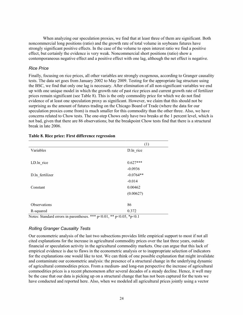
Finally, focusing on rice prices, all other variables are strongly exogenous, according to Granger causality tests. The data set goes from January 2002 to May 2009. Testing for the appropriate lag structure using the BSC, we find that only one lag is necessary. After elimination of all non-significant variables we end up with one unique model in which the growth rate of past rice prices and current growth rate of fertilizer prices remain significant (see Table 8). This is the only commodity price for which we do not find evidence of at least one speculation proxy as significant. However, we claim that this should not be surprising as the amount of futures trading on the Chicago Board of Trade (where the data for our speculation proxies come from) is much smaller for this commodity than the other three. Also, we have concerns related to Chow tests. The one-step Chows only have two breaks at the 1 percent level, which is not bad, given that there are 86 observations; but the breakpoint Chow tests find that there is a structural break in late 2006.

Table 8. Rice price: First difference regression

(1) Variables D.ln_rice LD.ln_rice 0.627***

-0.0936

D.ln_fertilizer -0.0764**

-0.014

Constant 0.00462

(0.00627)

Observations 86 R-squared 0.372

Notes: Standard errors in parentheses. *** p<0.01, ** p<0.05, *p<0.1

Rolling Granger Causality Tests

Our econometric analysis of the last two subsections provides little empirical support to most if not all cited explanations for the increase in agricultural commodity prices over the last three years, outside financial or speculation activity in the agricultural commodity markets. One can argue that this lack of empirical evidence is due to flaws in the econometric analysis or to inappropriate selection of indicators for the explanations one would like to test. We can think of one possible explanation that might invalidate and contaminate our econometric analysis: the presence of a structural change in the underlying dynamic of agricultural commodities prices. From a medium- and long-run perspective the increase of agricultural commodities prices is a recent phenomenon after several decades of a steady decline. Hence, it well may be the case that our data is picking up on a structural change that has not been captured for the tests we have conducted and reported here. Also, when we modeled all agricultural prices jointly using a vector

25

ECM, we were not able to find a cointegration vector or long-run regression for the sample period 2002–2009; however, we did find cointegrating vectors, although different ones, when analyzing subperiods, which also may suggest the presence of a change in the underlying dynamic of prices. To face this possibility we decided to run rolling windows Granger causality tests for all our candidate variables that might help explain the evolution of agricultural prices.

The rolling windows Granger causality tests we conduct here work in the following way. First, we take the first 30 months available in our sample period, from January 2002 through June 2004, and test for Granger causality of a given variable on the price of an agricultural commodity. Second, we roll the sample period one month ahead, from February 2002 through July 2004, and redo the Granger causality test. Third, we roll the sample one extra month and test again. We keep rolling the sample window in a similar manner until the last window ends in March 2008. We execute this procedure testing for Granger causality of every available variable on each and all four agricultural prices. We remind the reader that a Granger causality test analyzes commodity prices based on past prices of that commodity and one other exogenous variable in its lags only. The appropriate lag structure (according to BSC) is used, and then a likelihood ratio test is used to compare the model including the exogenous variable and the model without it. A significant F statistic implies that there is Granger causality in the sense that the exogenous variable being tested can be used, for a particular block of time, as a predictor of future growth rates of the commodity price. Hence, this way we expect to capture if some of our variables can be regarded as Granger-causing prices at least for some sub-periods between years 2002 and 2009. And we pay particular attention to variables that although not Granger-causing prices at the beginning of our sample, say, years 2002 through 2004, they show evidence of Granger-causing prices in the most recent 30 months of our sample period (from 2005 onward).

We report here only those cases in which we find any evidence of Granger causality in any period. Our reports take the form of a graph where we report the F-statistic of the corresponding Granger causality test, for each rolling window over time, and compare it with the critical F-value. Whenever the F-statistic goes above the critical F-value then evidence of Granger causality is found. In what follows we skip tests using speculation proxies; we leave those to the end of this subsection.

First, we analyze all exogenous variables on wheat prices and find that most series do not Granger-cause prices for any window of time. We only find weak evidence that biodiesel production and exports do start to Granger-cause prices in the most recent periods. In the case of wheat exports we find evidence of Granger causality only when the rolling windows reach September, October, November, and December of 2007.

Figure 16. Wheat exports Granger-cause wheat prices

0

1

2

3

4

5

6

7

8

Apr

-04

Jul-0

4

Oct

-04

Jan-

05

Apr

-05

Jul-0

5

Oct

-05

Jan-

06

Apr

-06

Jul-0

6

Oct

-06

Jan-

07

Apr

-07

Jul-0

7

Oct

-07

Jan-

08

Apr

-08

Jul-0

8

Oct

-08

Jan-

09

Apr

-09

wheatexp t1

26

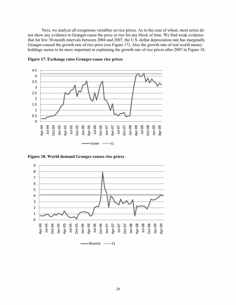
Next, we analyze all exogenous variables on rice prices. As in the case of wheat, most series do not show any evidence to Granger-cause the price or rise for any block of time. We find weak evidence that for few 30-month intervals between 2004 and 2007, the U.S. dollar depreciation rate has marginally Granger-caused the growth rate of rice price (see Figure 17). Also the growth rate of real world money holdings seems to be more important in explaining the growth rate of rice prices after 2007 in Figure 18.

Figure 17. Exchange rates Granger-cause rice prices

Figure 18. World demand Granger-causes rice prices

0

0.5

1

1.5

2

2.5

3

3.5

4

4.5

Apr

-04

Jul-0

4

Oct

-04

Jan-

05

Apr

-05

Jul-0

5

Oct

-05

Jan-

06

Apr

-06

Jul-0

6

Oct

-06

Jan-

07

Apr

-07

Jul-0

7

Oct

-07

Jan-

08

Apr

-08

Jul-0

8

Oct

-08

Jan-

09

Apr

-09

riceer t1

0

1

2

3

4

5

6

7

8

9

Apr

-04

Jul-0

4

Oct

-04

Jan-

05

Apr

-05

Jul-0

5

Oct

-05

Jan-

06

Apr

-06

Jul-0

6

Oct

-06

Jan-

07

Apr

-07

Jul-0

7

Oct

-07

Jan-

08

Apr

-08

Jul-0

8

Oct

-08

Jan-

09

Apr

-09

Ricem2 t1

27

When we analyze the price of soybeans, we find that starting in mid-2005 (which implies a 30-month period ending by December 2007), the growth rate in the world exports of soybeans shows evidence of Granger causing the growth rate of soybean prices (see Figure 19). However this evidece is only present for that specific period Also the growth rate of oil prices shows some weak evidence of Granger causing the growth rate of soybean prices at different periods over the last five years (see Figure 20). No other variable shows evidence of Granger causality.

Figure 19. Soybean exports Granger-cause soybean prices

Figure 20. Oil prices Granger-cause soybean prices

00.5

11.5

22.5

33.5

44.5

5

Apr

-04

Jul-0

4

Oct

-04

Jan-

05

Apr

-05

Jul-0

5

Oct

-05

Jan-

06

Apr

-06

Jul-0

6

Oct

-06

Jan-

07

Apr

-07

Jul-0

7

Oct

-07

Jan-

08

Apr

-08

Jul-0

8

Oct

-08

Jan-

09

Apr

-09

Soyexp t1

0

1

2

3

4

5

Apr

-04

Jul-0

4

Oct

-04

Jan-

05

Apr

-05

Jul-0

5

Oct

-05

Jan-

06

Apr

-06

Jul-0

6

Oct

-06

Jan-

07

Apr

-07

Jul-0

7

Oct

-07

Jan-

08

Apr

-08

Jul-0

8

Oct

-08

Jan-

09

Apr

-09

Soyoil t1

28

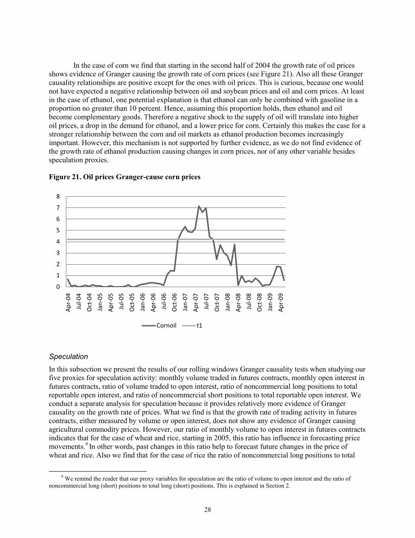
In the case of corn we find that starting in the second half of 2004 the growth rate of oil prices shows evidence of Granger causing the growth rate of corn prices (see Figure 21). Also all these Granger causality relationships are positive except for the ones with oil prices. This is curious, because one would not have expected a negative relationship between oil and soybean prices and oil and corn prices. At least in the case of ethanol, one potential explanation is that ethanol can only be combined with gasoline in a proportion no greater than 10 percent. Hence, assuming this proportion holds, then ethanol and oil become complementary goods. Therefore a negative shock to the supply of oil will translate into higher oil prices, a drop in the demand for ethanol, and a lower price for corn. Certainly this makes the case for a stronger relationship between the corn and oil markets as ethanol production becomes increasingly important. However, this mechanism is not supported by further evidence, as we do not find evidence of the growth rate of ethanol production causing changes in corn prices, nor of any other variable besides speculation proxies.

Figure 21. Oil prices Granger-cause corn prices

Speculation

In this subsection we present the results of our rolling windows Granger causality tests when studying our five proxies for speculation activity: monthly volume traded in futures contracts, monthly open interest in futures contracts, ratio of volume traded to open interest, ratio of noncommercial long positions to total reportable open interest, and ratio of noncommercial short positions to total reportable open interest. We conduct a separate analysis for speculation because it provides relatively more evidence of Granger causality on the growth rate of prices. What we find is that the growth rate of trading activity in futures contracts, either measured by volume or open interest, does not show any evidence of Granger causing agricultural commodity prices. However, our ratio of monthly volume to open interest in futures contracts indicates that for the case of wheat and rice, starting in 2005, this ratio has influence in forecasting price movements.9

9 We remind the reader that our proxy variables for speculation are the ratio of volume to open interest and the ratio of

noncommercial long (short) positions to total long (short) positions. This is explained in Section 2.

In other words, past changes in this ratio help to forecast future changes in the price of wheat and rice. Also we find that for the case of rice the ratio of noncommercial long positions to total

0

1

2

3

4

5

6

7

8

Apr

-04

Jul-0

4

Oct

-04

Jan-

05

Apr

-05

Jul-0

5

Oct

-05

Jan-

06

Apr

-06

Jul-0

6

Oct

-06

Jan-

07

Apr

-07

Jul-0

7

Oct

-07

Jan-

08

Apr

-08

Jul-0

8

Oct

-08

Jan-

09

Apr

-09

Cornoil t1

29

long (reportable) positions has an effect on prices, starting in 2004. When we analyze the same ratio for short positions, we find additional evidence for speculation affecting the growth rate of corn and soybean prices. In the case of corn there are signs of causality between March 2004 and September 2006 and during the 30-month span lasting from May 2005 until November 2007. In the case of soybeans we find weak evidence, in particular for the 30-month period ending February 2008. In Figure 2 we put together all these results; notice that the vertical axis shows the difference between the F-critical value and the F-statistic of our Granger causality test such that positive values of these differences indicate evidence of causality.

Interestingly as the rolling samples include 2008 and 2009 data, picking the decrease of grain prices since mid 2008 and the adverse effects of the global financial crisis, the evidence of speculation activity affecting spot prices vanishes in all cases we presented. This is interesting and supports the view that during the food crisis agricultural grain markets were operating under a different regime in which speculation activity played a role in spot prices formation. Notice that it is important to emphasize the idea of a different regime because otherwise we wouldn’t observe such drastic changes in granger causality tests as we roll out our samples out of the food crisis period. To say that speculative activity decreased after mid 2008 is not enough to get to observe the vanishing effects of granger causality tests, all the contrary it would have helped the econometric regressions to link changes in the speculation proxies to changes in the growth rate of prices. The overall evidence points then to the following interpretation: before and after the food crisis speculation activity had no effect on spot prices formation while during the crisis it did. This is not to say that before and after the crisis speculation was not present, it was (probably to a less extent) but didn’t granger cause spot prices.

Figure 22. Granger causality: Speculation proxies

-5

-4

-3

-2

-1

0

1

2

3

4

5

Apr

-04

Aug

-04

Dec

-04

Apr

-05

Aug

-05

Dec

-05

Apr

-06

Aug

-06

Dec

-06

Apr

-07

Aug

-07

Dec

-07

Apr

-08

Aug

-08

Dec

-08

Apr

-09

Inde

x =

F st

atis

tic

-F c

riti

cal v

alue

Last month of a 30-months period

Evidence of speculation influencing commodity prices

(positive numbers on vertical axis shows evidence of influence)

Wheat: Volume/Open Interest

Rice: Volume/Open Interest

30

4. CONCLUDING REMARKS

From 2006 to mid 2008 the international prices of agricultural commodities increased considerably, by a factor larger than two. This upward trend in agricultural prices caught the world’s attention as a new food crisis was emerging. Several explanations for these movements in prices, ranging from demand-driven forces to supply shocks, have been provided by analysts, researchers, and development institutions. In this paper we use a time series approach to empirically validate or reject these explanations using data at a monthly frequency. We focus on the international price of corn, wheat, rice, and soybeans. First, we identify variables associated with the factors mentioned as causing the increase in these agricultural commodities prices. Second, we use time series analysis to try to quantitatively validate those explanations. The empirical work presented here relies on single equations first difference models and rolling Granger causality tests. Vector error correction models and single-equation error correction models were also analyzed, however we concluded that they are not effective models to represent agricultural commodities price dynamic. Overall, our empirical analysis mainly provides evidence that financial activity in futures markets and proxies for speculation can help explain the observed change in food prices; any other explanations are weakly or not well supported by our time series analysis.

When using first difference models, we find that in the case of corn three of our five speculation proxies show explanatory power in our regressions. The fraction of long positions in futures contracts by noncommercial traders, the fraction of short positions in futures contracts by noncommercial traders, and total open interest in corn futures contracts seem to partially explain corn price growth rate.

In the case of wheat prices we find evidence that the growth rate of wheat world exports (lagged one period) has a robust positive effect on the growth rate of wheat prices. In three of our models we find that the growth rate of worldwide real money supply has a positive effect on wheat prices, supporting the idea that world aggregate demand pressures might have a played a role in the acceleration of wheat price increments. Also, in two specifications, lagged growth rate of oil has a positive effect on the growth rate of wheat prices. However, at the same time the growth rate of ethanol and biodiesel production do not show as significant explanatory variables. When we turn our attention to our speculation proxies, we get stronger evidence because all our proxies in one or another specification enter as significant.

When analyzing the price of soybeans we find evidence of four variables, other than our speculation proxies, as having explanatory power on the growth rate of soybean prices. Contrary to what we have expected, we find a negative effect coming from the growth rate of oil prices. The contemporaneous growth rate of soybeans exports has a positive effect on all five regressions with relatively stable coefficients across specifications. In all regressions we find that the dollar depreciation is transmitted to the dollar price of soybeans, and the evidence shows that at least 50 percent of such depreciation is transmitted, and we even have a specification in which the transmission is one-to-one with one lag. This seems to indicate that the determination of soybean prices takes place in a different currency than the U.S. dollar. Also we find weak evidence that the growth rate of fertilizer prices has a positive effect, although the significance level of this effect is very low. When analyzing our speculation proxies we conclude that at least three of them are significant. Both noncommercial long positions (ratio) and the growth rate of total volume in soybeans futures have strongly significant positive effects. In the case of the volume to open interest ratio we find a positive effect, but certainly the evidence is very weak.

For rice prices we find that only the current growth rate of fertilizer prices is significant. This is the only commodity price for which we do not find evidence of at least one speculation proxy as significant when using single-equation first difference models. However, we claim that this should not be surprising considering that the amount of futures trading on the Chicago Board of Trade (where the data for our speculation proxies come from) is much smaller for this commodity than the other three.

Because we were concerned about the lack of strong support for explanations of high food prices other than activity and/or speculation in the futures markets, we evaluated the possibility that our econometric analysis was contaminated by the presence of structural change in the underlying dynamic of agricultural commodity prices. In fact from a medium- and long-run perspective, the increase of

31

agricultural commodities prices is a recent phenomenon after several decades of a steady decline. Hence, it well may be the case that our data is picking up on a structural change that has not been captured by the tests we have conducted. In order to face this possibility we decided to run rolling windows Granger causality tests for all our candidate variables that might help explain the evolution of agricultural prices.

Results of our rolling windows Granger causality tests show the following: (1) In the case of rice prices we find weak evidence that for few 30-month intervals between 2004 and 2007, the U.S. dollar depreciation rate has marginally Granger-caused the growth rate of rice price; and also the growth rate of real world money holdings seems to be more important in explaining the growth rate of rice prices after 2004, but this evidence is not really statistically significant. (2) When we analyze the price of soybeans we find that, starting in mid-2005 (which implies a 30-month period ending December 2007), the growth rate in the world exports of soybeans shows evidence of Granger causing the growth rate of soybean prices. (3) In the case of corn we find that starting in the second half of 2004 the growth rate of oil prices shows evidence of Granger causing the growth rate of corn prices, but with a negative relationship. (4) When analyzing our speculation proxies we observe that the ratio of monthly volume to open interest in futures contracts indicates that for the case of wheat and rice, starting in 2005, it has influence in forecasting price movements. Also we find that for the case of rice, the ratio of noncommercial long positions to total long (reportable) positions has an effect on prices, starting in 2004. When we analyze the same ratio for short positions we find additional evidence for speculation affecting the growth rate of corn and soybean prices. In the case of corn there are signs of causality between March 2004 and September 2006, and during the 30-month span from May 2005 to November 2007. In the case of soybeans we find weak evidence, in particular for the 30-month period ending February 2008.

Interestingly as the rolling samples include 2008 and 2009 data, picking the decrease of grain prices since mid 2008 and the adverse effects of the global financial crisis, the evidence of speculation activity affecting spot prices vanishes in all cases. This supports the view that during the food crisis agricultural grain markets were operating under a different regime in which speculation activity played a role in spot prices formation. The overall evidence points to the following interpretation: before and after the food crisis speculation activity had no effect on spot prices formation while during the crisis it did. This is not to say that before and after the crisis speculation was not present, it was (probably to a less extent) but didn’t granger cause spot prices.

Overall, we conclude from our time series analysis that when taking the four commodities analyzed here there is evidence that financial activity in futures markets and/or speculation in these markets can help explain the behavior of these prices in recent years. Other explanations are only partially supported for the particular case of one agricultural commodity or not supported at all. We do not claim, however, that these other explanations should be disregarded; all that we can say is that in using the variables considered in this study and the particular time series models herein, we do not find such evidence.

32

APPENDIX

Chow Tests

Figure A.1. Chow tests (top: one-step, bottom: breakpoint) on whole set of full corn differencing equation

Figure A.2. Chow tests (top: one-step, bottom: breakpoint) on shortened set of full corn differencing equation

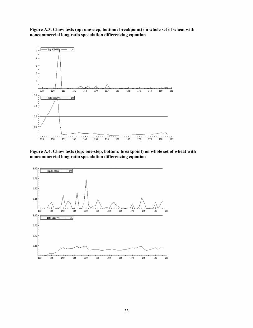
33

Figure A.3. Chow tests (op: one-step, bottom: breakpoint) on whole set of wheat with noncommercial long ratio speculation differencing equation

Figure A.4. Chow tests (top: one-step, bottom: breakpoint) on whole set of wheat with noncommercial long ratio speculation differencing equation

34

REFERENCES

Abbott, P. C., Hurt, C. & Tyner, W. E. 2008. What’s Driving Food Prices? Farm Foundation, Issue Report July 2008.

Brahmbhatt, M., and L. Christiaensen. 2008. Rising food prices in East Asia: Challenges and policy options.http://siteresources.worldbank.org/EASTASIAPACIFICEXT/Resources/EA_Rising_Food_Prices050508.pdf. Accessed on July 2008

Calvo, G. 2008, June 20. Exploding commodity prices, lax monetary policy, and sovereign wealth funds. VoxEU. http://www.voxeu.org/index.php?q=node/1244. Accessed on July 2008

Campbell, J. Y., A. W. Lo, and A. C. MacKinlay. 1996. The Econometrics of Financial Markets. Princeton University Press.

Chicago Board of Trade. 2008a. An Introduction to trading CBOT agricultural futures and options.

———. 2008b. A hedger's self-study guide.

———. 2008c. Trading in futures: An introduction.

Coady, D., P. Dorosh, and B. Minten. 2008. Evaluating alternative policy responses to higher world food prices: The case of increasing rice prices in Madagascar. IFPRI Discussion Paper 780. Washington, D.C: International Food Policy Research Institute.

Collier, P. 2007. Managing commodity booms: Lessons of international experience. Paper prepared for the African Economic Research Consortium, January 2007.

Fan, S., and M. W. Rosegrant. 2008. Investing in agriculture to overcome the world food crisis and reduce poverty and hunger. IFPRI Policy Brief 3, 4 pages

FAO. 2008a. Crop prospects and food situation. No. 3. July.

———. 2008b. Soaring food prices: Facts, perspectives, impacts and actions required. Document prepared for the High-level conference on world security: The challenges of climate change and bioenergy, Rome 3-5 June

Gilbert, C. 2008. Trends and volatility in agricultural commodity prices. In Agricultural commodity markets and trade: New approaches to analyzing market structure and instability. Ed. A. Sarris and Hallam D. (pp 31-60). FAO/Edward Elgar Publishing.

Hamilton, J. D. 1994. Time series analysis. Princeton University Press.

Headey, D., and S. R. Skorbiansky. 2008. International food crises, past and present: A comparison of causes and consequences. IFPRI Discussion Paper 00831

Hull, J. C. 2008. Options, futures, and other derivatives. 6 ed. Prentice Hall.

IMF Fiscal Affairs, Policy Development and Review, and Research Departments. 2008. Food and fuel prices: Recent developments, macroeconomic impact, and policy responses. Approved by Teresa Ter-Minassian, Mark Allen, and Simon Johnson, June 30

International Grains Council. 2008. Grain market report. No. GMR No.378.

———. 2008. Grain market report. No. GMR No. 379.

Irwin 2008, S. H. Is speculation by long-only index funds harmful to commodity markets? Testimony before U.S. House Agriculture Committee, July 10, 2008. http://agriculture.house.gov/testimony/110/h80710/irwin.pdf. Accessed on February 2009

Irwin, S. H., P. Garcia, D. L. Good, and E. L. Kunda. 2008. Recent delivery performance of CBOT corn, soybean, and wheat futures contracts. Choices: The magazine of food, farm, and resource issues. 2nd Quarter 2008, 23(2) (pp 16-21).

Masters, M. W. 2008. Testimony of Michael W. Masters, managing member / portfolio manager masters, Capital Management, LLC, before the Committee on Homeland Security and Governmental Affairs United States Senate, May 20, 2008. http://hsgac.senate.gov/public/_files/052008Masters.pdf. Accessed on March 2009.

http://siteresources.worldbank.org/EASTASIAPACIFICEXT/Resources/EA_Rising_Food_Prices050508.pdf�

http://siteresources.worldbank.org/EASTASIAPACIFICEXT/Resources/EA_Rising_Food_Prices050508.pdf�

http://www.voxeu.org/index.php?q=node/1244�

http://agriculture.house.gov/testimony/110/h80710/irwin.pdf.%20Accessed%20on%20February%202009�

http://hsgac.senate.gov/public/_files/052008Masters.pdf�

35

Ivanic, M., and W. Martin. 2008. Implications of higher global food prices for poverty in low-income countries. Policy Research Working Paper. The World Bank Development Research Group - Trade Team.

Krugman, P. 2008. Speculative nonsense, once again. New York Times. June 23. http://krugman.blogs.nytimes.com/2008/06/23/speculative-nonsense-once-again/. Accessed on July 2008.

Latin American Shadow Financial Regulatory Committee. 2008. Sailing in a stormy sea: Latin America's response to global financial turmoil and the food price crisis. Statement No. 18.

Mitchell, D. 2008. A note on rising food prices. Policy Research Working Paper No. 4682. The World Bank, Washington, D.C.

OECD Policy Report. 2008. Rising food prices: Causes and consequences. http://www.oecd.org/dataoecd/54/42/40847088.pdf. Accessed on July 2008

Rojas-Suarez, L. 2008. The right response in Latin America to oil and food price pressures: Fight inflation now! Center For Global Development Essay, August. www.cgdev.org/publications/detail/16531. Accessed on August 2008.

Sanders, D. R., S. H. Irwin, and R. P. Merrin. 2008. The adequacy of speculation in agricultural futures markets: Too much of a good thing? Marketing and Outlook Research Report 2008-02. Department of Agricultural and Consumer Economics, University of Illinois at Urbana-Champaign, June. http://www.farmdoc.uiuc.edu/marketing/morr/morr_archive.html. Accessed on Jan 2009.

Sommer, M., and C. Gilbert. 2006. The boom in nonfuel commodity prices: Can it last? In World Economic Outlook. 35.

Trostle, R. 2008. Global agricultural supply and demand: Factors contributing to the recent increase in food commodity prices. USDA Economic Research Service Report No. WRS-0801.

UNCTAD Policy Brief. 2008. Tackling the global food crisis. No. 2.

UNCTAD.2008. Addressing the global food crisis: Key trade, investment and commodity policies in ensuring sustainable food security and alleviating poverty. Prepared for the High-level conference on world security: The challenges of climate change and bioenergy, Rome 3-5 June.

Valdes, A., and W. Foster. 2008. High world commodity prices hurt or help family farms? A simulation case study for Chile. Prepared for FAO Expert Workshop on Policies for the Effective Management of Sustained Food Price Increases in Rome, July 2008.

Von Braun, J. 2007. The world food situation: New driving forces and required actions. International Food Policy Research Institute Food Policy Report No. 18, December 2007.

von Braun, J. 2008a. Food summit: Some progress but more needs to be done. IFPRI Press Release June 6, 2008.

———. 2008b. Biofuels, international food prices, and the poor. Testimony before the United States Senate Committee on Energy and Natural Resources, June 12.

———. 2008c. Rising food prices: What should be done? International Food Policy Research Institute Policy Brief, April 2008.

von Braun, J., et al. 2008. High food prices: The what, who, and how of proposed policy actions. IFPRI Policy Brief, May 2008.

von Braun, J., and T. Maximo. 2008. Physical and virtual global food reserves to protect the poor and prevent market failure. International Food Policy Research Institute Policy Brief No. 004.

World Agricultural Outlook Board. 2008. World agricultural supply and demand estimates. No. WASDE-460.

World Bank. 2008. G8 Hokkaido-Toyako summit: Double jeopardy: Responding to high food and fuel prices.

World Bank 2008. Rising food prices: Policy options and World Bank response.

http://siteresources.worldbank.org/NEWS/Resources/risingfoodprices_backgroundnote_apr08.pdf. Accessed on July 2008.

http://krugman.blogs.nytimes.com/2008/06/23/speculative-nonsense-once-again/�

http://www.oecd.org/dataoecd/54/42/40847088.pdf�

http://www.cgdev.org/publications/detail/16531�

http://www.farmdoc.uiuc.edu/marketing/morr/morr_archive.html�

http://siteresources.worldbank.org/NEWS/Resources/risingfoodprices_backgroundnote_apr08.pdf�

RECENT IFPRI DISCUSSION PAPERS

For earlier discussion papers, please go to http://www.ifpri.org/category/publication-type/discussion-papers. All discussion papers can be downloaded free of charge.

941. Decentralization, agricultural services and determinants of input use in Nigeria. Kamiljon T. Akramov, 2009.

940. How important are peer effects in group lending? Estimating a static game of incomplete information. Shanjun Li, Yanyan Liu, and Klaus Deininger, 2009.

939. Rice production responses in Cambodia. Bingxin Yu and Shenggen Fan, 2009.

938. A latent class approach to investigating consumer demand for genetically modified staple food in a developing country: The case of gm bananas in Uganda. Enoch Kikulwe, Ekin Birol, Justus Wesseler, and José Falck-Zepeda, 2009.

937. Cluster-based industrialization in China: Financing and performance. Cheryl Long and Xiaobo Zhang, 2009.

936. Sensitivity of welfare effects estimated by equilibrium displacement model: A biological productivity growth for semisubsistence crops in Sub-Sahara African market with high transaction costs. Hiroyuki Takeshima, 2009.

935. Assessing household vulnerability to climate change: The case of farmers in the Nile Basin of Ethiopia. Temesgen T. Deressa, Rashid M. Hassan, and Claudia Ringler, 2009.

934. Do external grants to district governments discourage own-revenue generation?: A look at local public finance dynamics in Ghana. Tewodaj Mogues, Samuel Benin, and Godsway Cudjoe, 2009.

933. Impacts of prenatal and environmental factors on child growth: Evidence from Indonesia. Futoshi Yamauchi, Katsuhiko Higuchi, and Rita Nur Suhaeti, 2009.

932. Rich consumers and poor producers: Quality and rent distribution in global value chains. Johan F.M. Swinnen and Anneleen Vandeplas, 2009.

931. Economic growth and distribution of income: A Growth model to fit Ghanaian data. Harumi T. Nelson , Terry L. Roe, and Xinshen Diao, 2009.

930. Trade liberalization, poverty, and food security in India. Manoj Panda and A. Ganesh-Kumar, 2009.

929. Improving the proof: Evolution of and emerging trends in impact assessment methods and approaches in agricultural development. Mywish K. Maredia, 2009.

928. Improving diet quality and micronutrient nutrition: Homestead food production in Bangladesh. Lora Iannotti, Kenda Cunningham, and Marie Ruel, 2009.

927. Land-tenure policy reforms: Decollectivization and the Doi Moi System in Vietnam. Michael Kirk and Tuan Nguyen, 2009.

926. “Crossing the river while feeling the rocks:” Incremental land reform and its impact on rural welfare in China. John W. Bruce and Zongmin Li, 2009.

925. Rich food for poor people: Genetically improved tilapia in the Philippines. Sivan Yosef, 2009.

924 .Rural and urban linkages: Operation Flood’s role in India’s dairy development. Kenda Cunningham, 2009.

923. The global effort to eradicate rinderpest. Peter Roeder and Karl Rich, 2009.

922. The mungbean transformation: Diversifying crops, defeating malnutrition. Subramanyan Shanmugasundaram, J. D. H. Keatinge, and Jacqueline d’Arros Hughes, 2009.

921. Private sector responses to public investments and policy reforms: The case of fertilizer and maize market development in Kenya. Joshua Ariga and T. S. Jayne, 2009.

920. Institutional reform in the Burkinabè cotton sector and its impacts on incomes and food security: 1996–2006. Jonathan Kaminski, Derek Headey, and Tanguy Bernard, 2009.

919. Pearl millet and sorghum improvement in India. Carl E. Pray and Latha Nagarajan, 2009.910. Combating stem and leaf rust of wheat: Historical perspective, impacts, and lessons learned. H. J. Dubin and John P. Brennan, 2009.

918. Hybrid rice technology development: Ensuring China’s food security. Jiming Li, Yeyun Xin, and Longping Yuan, 2009.

917. The impact of shallow tubewells and boro rice on food security in Bangladesh. Mahabub Hossain, 2009.

http://www.ifpri.org/category/publication-type/discussion-papers�

INTERNATIONAL FOOD POLICY RESEARCH INSTITUTE

www.ifpri.org

IFPRI HEADQUARTERS

2033 K Street, NW Washington, DC 20006-1002 USA Tel.: +1-202-862-5600 Fax: +1-202-467-4439 Email: [email protected]

IFPRI ADDIS ABABA

P. O. Box 5689 Addis Ababa, Ethiopia Tel.: +251 11 6463215 Fax: +251 11 6462927 Email: [email protected]

IFPRI NEW DELHI

CG Block, NASC Complex, PUSA New Delhi 110-012 India Tel.: 91 11 2584-6565 Fax: 91 11 2584-8008 / 2584-6572 Email: [email protected]


bryce cooke miguel robles - international food policy research

Documents