bsml: a binding schema markup language for data ...people.cs.vt.edu/naren/papers/bsmlpaper.pdfbsml:...

BSML: A Binding Schema Markup Language forData Interchange in Problem Solving Environments∗

Alex Verstak∗, Naren Ramakrishnan∗, Layne T. Watson∗, Jian He∗, Clifford A. Shaffer∗,Kyung Kyoon Bae†, Jing Jiang†, William H. Tranter†, and Theodore S. Rappaport†

∗Department of Computer Science†Bradley Department of Electrical and Computer Engineering

Virginia Polytechnic Institute and State UniversityBlacksburg, Virginia 24061Contact: [email protected]

Abstract

We describe a binding schema markup language (BSML) for describing data interchange between scientific codes.Such a facility is an important constituent of scientific problem solving environments (PSEs). BSML is designedto integrate with a PSE or application composition system that views model specification and execution as aproblem of managing semistructured data. The data interchange problem is addressed by three techniques forprocessing semistructured data: validation, binding, and conversion. We present BSML and describe its applica-tion to a PSE for wireless communications system design.

1 Introduction

Problem solving environments (PSEs) are high-level software systems for doing computational science. A simpleexample of a PSE is the Web PELLPACK system [20] that addresses the domain of partial differential equations(PDEs). Web PELLPACK allows the scientist to access the system through a Web browser, define PDE problems,choose and configure solution strategies, manage appropriate hardware resources (for solving the PDE), and visualizeand analyze the results. The scientist thus communicates with the PSE in the vernacular of the problem, ‘not in thelanguage of a particular operating system, programming language, or network protocol’ [16]. It is 10 years sincethe goal of creating PSEs was articulated by an NSF workshop (see [16] for findings and recommendations). Fromproviding high-level programming interfaces for widely used software libraries [22], PSEs have now expanded todiverse application domains such as wood-based composites design [18], aircraft design [17], gas turbine dynamicssimulation [15], and microarray bioinformatics [4].

The basic functionalities expected of a PSE include supporting the specification, monitoring, and coordinationof extended problem solving tasks. Many PSE system designs employ the compositional modeling paradigm, wherethe scientist describes data-flow relationships between codes in terms of a graphical network and the PSE managesthe details of composing the application represented by the network. Compositional modeling is not restricted tosuch model specification and execution but can also be used as an aid in performance modeling of scientific codes [2](model analysis).

We view model specification and execution as a data management problem and describe how a semistructureddata model can be used to address data interchange problems in a PSE. Section 1.1 presents a motivating PSE sce-nario that will help articulate needs from a data management perspective. Section 2 elaborates on these ideas and

∗The work presented in this paper is supported in part by National Science Foundation grants EIA-9974956, EIA-9984317, and EIA-0103660.

1

briefly reviews pertinent related work. In particular, it identifies three basic levels of functionality—validation, bind-ing, and conversion—at which data interchange in application composition can be studied. Sections 4, 5, and 6 de-scribe our specific contributions along these dimensions, in the form of a binding schema markup language (BSML).Section 7 outlines how these ideas can be integrated within an existing PSE system design. A concluding discus-sion is provided in Section 8. Aspects of the scenario described next will be used throughout this paper as runningexamples.

1.1 Motivating Example

S4W (Site-Specific System Simulator for Wireless system design) is a PSE being developed at Virginia Tech. S4Wprovides deterministic electromagnetic propagation and stochastic wireless system models for predicting the perfor-mance of wireless systems in specific environments, such as office buildings. S4W is also designed to support theinclusion of new models into the system, visualization of results produced by the models, integration of optimiza-tion loops around the models, validation of models by comparison with field measurements, and management of theresults produced by a large series of experiments. S4W permits a variety of usage scenarios. We will describe onescenario in detail.

A wireless design engineer uses S4W to study transmitter placement in an indoor environment located on thefourth floor of Durham Hall at Virginia Tech. The engineering goal is to achieve a certain performance objectivewithin the given cost constraints. For a narrowband system, power levels at the receiver locations are good indicatorsof system performance. Therefore, minimizing the (spatial) average shortfall of received power with respect tosome power threshold is a meaningful and well defined objective. The major cost constraints are the number oftransmitters and their powers. Different transmitter locations and powers yield different levels of coverage. Thesituation is more complicated in a wideband system, but roughly the same process applies. A wideband systemincludes extra hardware not present in a narrowband system and the performance objective is formulated in terms ofthe bit error rate (BER), not just the power level.

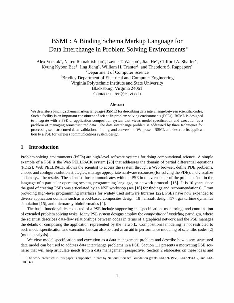
The first step in this scenario is to construct a model of signal propagation through the wireless communicationschannel. S4W provides ray tracing as the primary mechanism to model site-specific propagation effects such astransmission (penetration), reflection, and diffraction. The second step is to take into account antenna parametersand system resolution. These two steps are often sufficient to model the performance of a narrowband system.If a wideband system is being considered, the third step is to configure the specific wireless system. Parameterssuch as the number of fingers of the rake receiver and forward error correction codes are considered at this step.S4W provides a Monte-Carlo simulation of a WCDMA (wideband code division multiple access) family of wirelesssystems. In either case, the engineer configures a graph of computational components as shown in Fig. 1. The ovalscorrespond to computational components drawn from a mix of languages and environments. Hexagons encloseinput and output data. Aggregation is used to simplify the interfaces of the components to each other and to theoptimizer. In Fig. 1, rectangles represent aggregation. The propagation model is a component that consists of threeconnected subcomponents: triangulation, space partitioning, and ray tracing. Similarly, the wireless system modelconsists of (roughly) three components: data encoding, channel modeling, and signal decoding. All three steps arefurther aggregated into a complete site-specific system model. This model is then used in an optimization loop.The optimizer changes transmitter parameters (all other parameters remain fixed) and receives feedback on systemperformance.

For a given environment definition in AutoCAD, the triangulation and space partitioning components are usedto reduce the number of geometric intersection tests that will be performed by the ray tracer. Several iterationsover space partitioning are necessary to achieve acceptable software performance. However, once the objective (anaverage of ten triangles per voxel) is met, the space partitioning can be reused in all future experiments with thisenvironment. The engineer then configures the ray tracer to only capture reflection and transmission (penetration)

2

Triangulation Space Partitioning

Transmitter Params.

Ray Tracing

Receiver Locations Propagation Model

Environment Data

Channel ModelingData Encoding Signal Decoding

Post ProcessingSystem Resolution

Impulse Responses Performance Metric

Wireless System Model

Site−Specific System Model

Antenna Params.

Signal−to−Noise Ratios

Power Delay Profiles

Figure 1: A site-specific system model in S4W. The system model consists of a propagation model, an antennamodel (post processing), and a wireless system model.

y, m

806040200

30

20

10

x, m

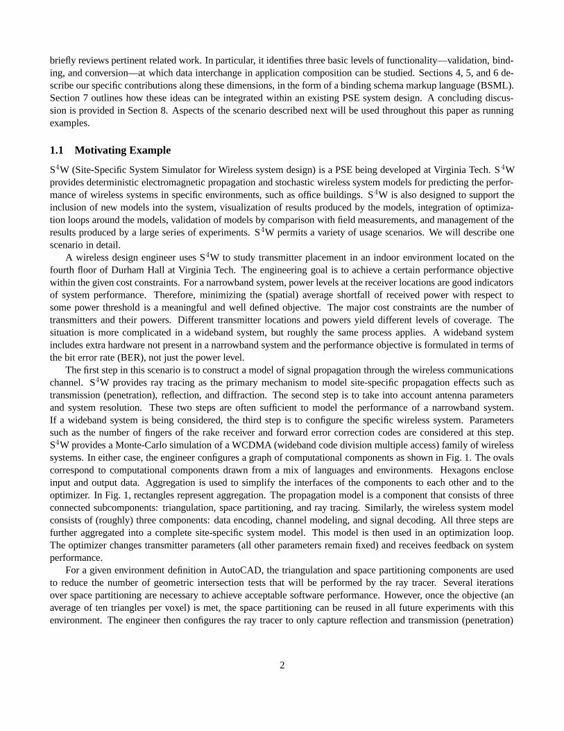
Figure 2: Optimizing placement of three transmitters to cover eighteen rooms and a corridor bounded by the boxin the upper left corner. The bounds for the placement of three transmitters are drawn with dotted lines. The initialtransmitter positions are marked with crosses. The optimum coverage transmitter positions are marked with dots.

effects. Although diffraction and scattering are important in indoor propagation [5], these phenomena are computa-tionally expensive to model in an optimization loop. The triangulation and space partitioning codes are meant forserial execution, whereas the ray tracer and the Monte Carlo wireless system models run on a 200 node Beowulfcluster of workstations. Post processing is available in both serial and parallel versions. The ray tracer and the postprocessor are written in C, whereas the WCDMA simulation is available in Matlab and Fortran 95 versions.

A series of experiments is performed for various choices of antenna patterns, path loss parameters (influenced bymaterial properties), and WCDMA system parameters. The predicted power delay profiles (PDPs) are then comparedwith the measurements from a channel sounder and the predicted bit error rates are compared with the publisheddata. The parameters of the propagation model are calibrated for various locations. The validated propagation andwireless system models are finally enclosed in an optimization loop to determine the locations of transmitters thatwill provide adequate performance for a region of interest. The optimizer, written in Fortran 95, uses the DIvidingRECTangles (DIRECT) algorithm of Jones et al. [19]. The parameters to the optimization problem and the optimaltransmitter placement are depicted in Fig. 2. The optimizer decided to move the transmitter in the upper right cornerone room to the right of its initial position and the transmitter in the lower left corner two rooms to the right of itsinitial position.

What requirements can we abstract from this scenario and how can they be flexibly supported by a data model?We first observe the diversity in the computational environment. Component codes are written in different languagesand some of them are meant for parallel execution. In a research project such as S4W, many components are underactive development, so their I/O specifications change over time. Second, the interconnection among components

3

is also flexible. Optimizing for power coverage and optimizing for bit error rate, while having similar motivations,require different topologies of computational components. Third, since different groups of researchers are involvedin the project, there exists significant cognitive discordance among vocabularies, data formats, components, andeven methodologies. For example, ray tracing models represent powers in a power delay profile in dBm (log scale).However, WCDMA models work with a normalized linear scale impulse response and an aggregate called the‘signal-to-noise ratio.’ Also, there is more than one way of calculating the signal-to-noise ratio. Since antennasgenerate noise that depends on their parameters, detailed antenna descriptions are necessary to calculate this ratio.However, researchers who are not concerned with antenna design seldom model the system at this level of detail.The typical practice is to use a fixed noise level in the calculations. Simulations of wireless systems abound in suchapproximations, ad hoc conversions, and simplifying assumptions.

2 PSE Requirements for Data Interchange

Culling from the above scenario, we arrive at a more formal list of data interchange requirements for applicationcomposition in a PSE. The PSE must support:

1. components in multiple languages (C, FORTRAN, Matlab, SQL);

2. changes in component interfaces;

3. changes in interconnections among components;

4. automatic unit conversion in data-flows;

5. user-defined conversion filters;

6. composition of components with slightly different interfaces; and

7. stream processing.

The reader might be surprised that SQL is listed alongside FORTRAN, but both languages are used in S4W.Experiment simulations are written in procedural languages, while experiment data is stored in a relational database.Thus, developing a system that integrates with the PSE environment requires more than the ability to link scientificcomputing languages. It involves overcoming the impedance mismatch between languages developed for fundamen-tally different purposes.

The last requirement above—stream processing—refers to processing data as soon as it is read from an inputstream, as opposed to waiting for the end of the stream, and subsequently processing all the data at once. This oftenneglected technical requirement is related to composability – the ability to create arbitrary component topologies.As data interchange is pushed deeper into the computation, the unit of data granularity needs to become correspond-ingly smaller. The optimization loop is a good example of fine data granularity. We cannot accumulate all transmitterparameters over all iterations and later convert them to the format required by the simulation inside the loop, becausetransmitter parameters generated by the optimizer depend on the feedback computed by the simulation. Each blockof transmitters must be processed as soon as it is available. Likewise, each value of the objective function must bemade available to the optimizer before it can produce the next block of transmitters. Usability dictates a similarrequirement. Since some models are computationally expensive (e.g., those meant for parallel execution), incre-mental feedback should be provided to the user as early as possible. The stream processing requirement improvescomposability and usability, but limits conversions to being local. Global conversions (e.g., XSLT [13]) cannot beperformed because they assume that all the data is available at once.

While the requirements point to a semistructured data model, no currently available data management systemsupports all forms of PSE functionality. This paper presents the prototype of such a system in the form of a markuplanguage. Observe that all of the above requirements are summarized by three standard techniques for workingwith semistructured data—validation, binding, and conversion. Validation establishes data conformance to a given

4

schema. It is a prerequisite to most of the requirements. Binding refers to integrating semistructured data withlanguages that were designed for different purposes (requirement 1). Conversion (transformation) takes care ofrequirements 2–6. Given two slightly different schemas, it is possible to generate an edit script [11] that convertsdata instances from one schema to another. Requirement 7 dictates that all such conversions must be local.

2.1 Related Work

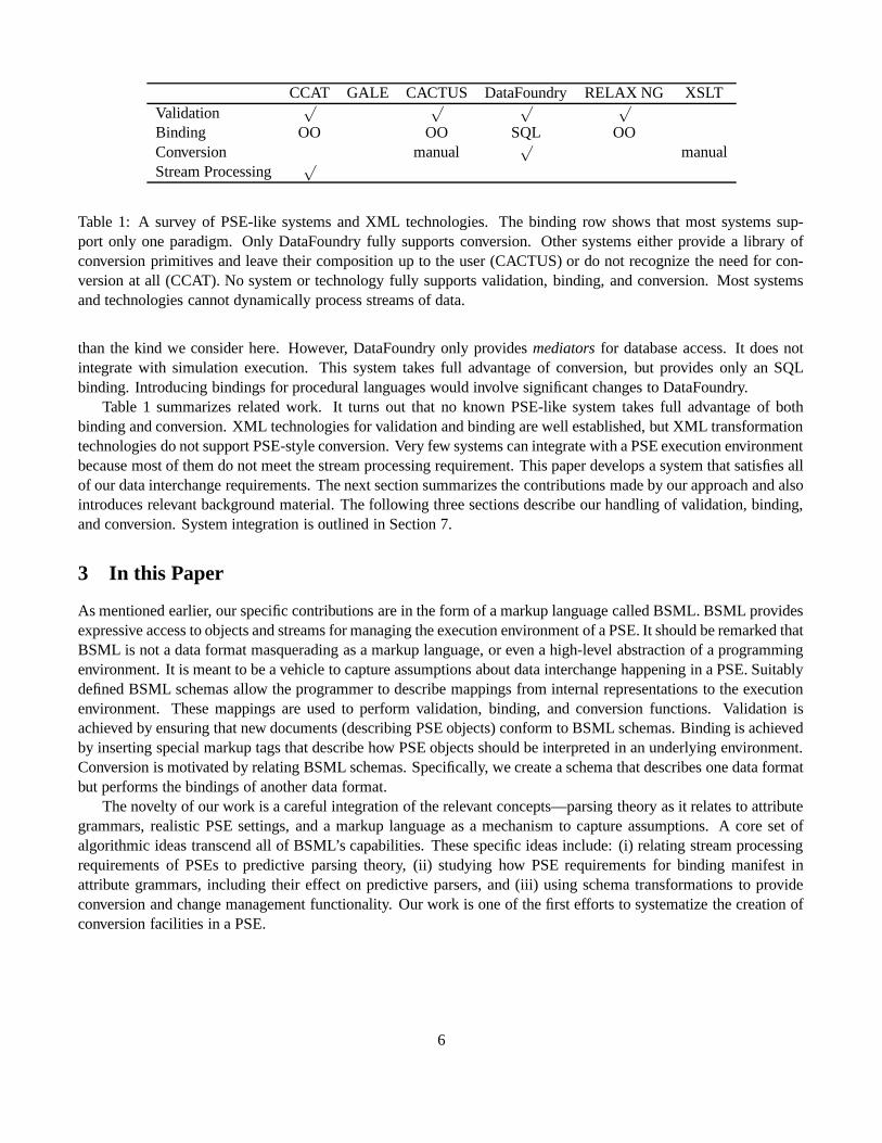
While research in PSEs covers a broad territory, the use of semistructured data representations in computationalscience is not established beyond a few projects. Therefore, we only survey standard XML technologies and PSE-like systems that make (some) use of semistructured data. It would be unfair to review some of these systems againstPSE data interchange requirements. Instead, our evaluation is based on how well these systems support validation,binding, conversion, and stream processing.

Specific XML technologies for document processing are easy to classify in terms of our framework. Schemalanguages (e.g., RELAX NG [12]) deal with validation and, possibly, binding. Transformation languages (e.g.,XSLT [13]) deal with conversion. Several properties of these technologies hinder their direct applicability to a PSEsetting. First and foremost, these technologies do not work with streams of data. Sophisticated schema constraintsand complex transformations can require buffering the whole document before producing any output. Second,transformation languages are simply vehicles for applying edit scripts. They cannot be used to create edit scripts.Since our conversions are local, edit script application is trivial, but edit script creation is not.

Four major flavors of PSE-like projects that use semistructured data representations can be identified:

1. component metadata projects;

2. workflow projects;

3. scientific data interchange projects; and

4. scientific data management projects.

Projects in the first category use XML to store IDL-like (interface definition language) component descriptionsand miscellaneous component execution parameters. An example of such a project is CCAT [9], which is a dis-tributed object oriented system. CCAT also uses XML for message transport between components, so we say thatit provides an OO binding. The second category of projects augments component metadata with workflow spec-ifications. For example, GALE [8] is a workflow specification language for executing simulations on distributedsystems. Unlike CCAT, GALE provides XML specifications for some common types of experiments, such as pa-rameter sweeps (CCAT uses a scripting language for workflow specification). However, GALE does not use XMLfor component data. Both the component metadata and workflow projects use XML to encode data that is notsemistructured. Their use of XML is not dictated by the need for automatic conversion. Neither generic bindingmechanisms nor conversion are provided by these projects.

The latter two groups of projects use XML for application data, not component metadata. Representatives ofthe scientific data interchange group develop flexible all-encompassing schemas for specific application domains.For example, CACTUS [7] deals with spatial grid data. CACTUS’s schema is complex enough to be consideredsemistructured and this project recognizes the need for conversion filters. However, it does not provide multiplelanguage support and, more importantly, does not accommodate changes in the schema. CACTUS’s conversionfilters aim at code reuse, not change management. This project has OO binding and manual conversion (the sequenceof conversions is not determined automatically). Complexity of the data format precludes stream processing.

Perhaps the most relevant group of projects for our purposes involves the scientific data management community.Especially interesting are the projects in rapidly evolving domains, such as bioinformatics. DataFoundry [1, 14] pro-vides a unifying database interface to diverse bioinformatics sources. Both the data and the schema of these sourcesevolve quickly, so DataFoundry has to deal with change management—by far more complex change management

5

CCAT GALE CACTUS DataFoundry RELAX NG XSLTValidation

√ √ √ √

Binding OO OO SQL OOConversion manual

√manual

Stream Processing√

Table 1: A survey of PSE-like systems and XML technologies. The binding row shows that most systems sup-port only one paradigm. Only DataFoundry fully supports conversion. Other systems either provide a library ofconversion primitives and leave their composition up to the user (CACTUS) or do not recognize the need for con-version at all (CCAT). No system or technology fully supports validation, binding, and conversion. Most systemsand technologies cannot dynamically process streams of data.

than the kind we consider here. However, DataFoundry only provides mediators for database access. It does notintegrate with simulation execution. This system takes full advantage of conversion, but provides only an SQLbinding. Introducing bindings for procedural languages would involve significant changes to DataFoundry.

Table 1 summarizes related work. It turns out that no known PSE-like system takes full advantage of bothbinding and conversion. XML technologies for validation and binding are well established, but XML transformationtechnologies do not support PSE-style conversion. Very few systems can integrate with a PSE execution environmentbecause most of them do not meet the stream processing requirement. This paper develops a system that satisfies allof our data interchange requirements. The next section summarizes the contributions made by our approach and alsointroduces relevant background material. The following three sections describe our handling of validation, binding,and conversion. System integration is outlined in Section 7.

3 In this Paper

As mentioned earlier, our specific contributions are in the form of a markup language called BSML. BSML providesexpressive access to objects and streams for managing the execution environment of a PSE. It should be remarked thatBSML is not a data format masquerading as a markup language, or even a high-level abstraction of a programmingenvironment. It is meant to be a vehicle to capture assumptions about data interchange happening in a PSE. Suitablydefined BSML schemas allow the programmer to describe mappings from internal representations to the executionenvironment. These mappings are used to perform validation, binding, and conversion functions. Validation isachieved by ensuring that new documents (describing PSE objects) conform to BSML schemas. Binding is achievedby inserting special markup tags that describe how PSE objects should be interpreted in an underlying environment.Conversion is motivated by relating BSML schemas. Specifically, we create a schema that describes one data formatbut performs the bindings of another data format.

The novelty of our work is a careful integration of the relevant concepts—parsing theory as it relates to attributegrammars, realistic PSE settings, and a markup language as a mechanism to capture assumptions. A core set ofalgorithmic ideas transcend all of BSML’s capabilities. These specific ideas include: (i) relating stream processingrequirements of PSEs to predictive parsing theory, (ii) studying how PSE requirements for binding manifest inattribute grammars, including their effect on predictive parsers, and (iii) using schema transformations to provideconversion and change management functionality. Our work is one of the first efforts to systematize the creation ofconversion facilities in a PSE.

6

3.1 Some Pertinent Background

We begin by reviewing some pertinent background in the areas of markup languages and parsing theory. Markuplanguages, like XML, HTML, and SGML, use a tagged structure to describe documents. While the types andintended semantics of tags are fixed in a language like HTML, tags in XML do not have any pre-defined meaning.This allows us to rapidly prototype domain-specific markup languages (like BSML) and use document processingtools to harness descriptions in such languages. Ultimately, this availability of readymade software is what steersscientific computing researchers to a markup language-based solution.

One typical use of a markup language is for defining data formats. For instance, we can define a markup lan-guage for describing time series data. Domains such as bioinformatics abound in such markup languages. BSML’sapproach is to employ tags that will help realize data interchange functionality. There are even projects that encap-sulate a complete ontology in a markup language!

Documents in a markup language can be displayed, interpreted, and reasoned about in simple ways. For instance,a web browser uses the <B>...</B> tag structure in a HTML document to recognize when to render text in bold.Similarly, we can assign any suitable interpretation to a markup language in a PSE setting.

A markup language can be defined by its DTD (Document Type Definition) which declares what a well formeddocument should look like. Among other things, the DTD helps validate new documents, to see if they adhereto the markup specification. Other tools use DTDs to automatically generate parsers for interpreting documents.XML Schema is a newer approach for schema definition of XML documents and is widely believed to eventuallysupersede DTDs. BSML can actually be thought of as a schema language specifically designed for data interchangein PSEs.

Two technologies that are especially relevant here are DOM and SAX. DOM (Document Object Model) is an ob-ject model that uses a tree structure to represent an XML document. This internal tree structure can then be navigatedand manipulated to provide many facilities, e.g., searching the tree for the occurence of a given string, or rearrangingthe tree structure to produce a new document. The contrasting approach, SAX, is an event-based technology thatrelates parsing events back to an application, which can then use them to implement specific functionality. Manyparsing tools use either or both these approaches. The reader is referred to introductory resources such as [10] formore details.

Besides markup language basics, this paper assumes background knowledge of grammars and computer lan-guages, especially as encountered in a compilers course. The most important concepts are LL grammars and theconstruction of predictive parsing tables. For our purposes, an LL grammar is one that supports iterative and incre-mental parsing of input and as we will show, this is a necessary pre-requisite to achieve data interchange funtionality.The first ‘L’ denotes a ‘left-to-right’ scan and the second ‘L’ denotes that we are performing a leftmost derivation.We will devote considerable attention to LL(1) grammars which are LL with only one symbol of lookahead. Theseconcepts are well covered in [3].

4 Validation

The first function we study, validation, establishes conformance of a data instance to a given schema. It is a prereq-uisite to binding and conversion. (This definition of validation is a small part of the process of validation in a PSE,which is concerned with the larger issue of a model being appropriate to solve a given problem; but, it suffices forthe purpose of this paper.) The schemas for PSE data are easy to obtain since computational science traditionallyuses rigid data structures, not loosely formatted documents. Describing the data structures in terms of schemashas several benefits. First, language-neutral schemas allow for interoperability between different languages (seerequirement 1 in the previous section). Second, schemas facilitate database storage and retrieval. Third, appropriateschemas help assign interpretations to various data fields. It is such interpretation that makes automatic conversion

7

possible (requirements 2–6).What kind of validation is appropriate for PSE data? Requirement 7 calls for the most expressive schema

language that can be parsed by a stream parser. In other words, we are looking for a schema language that can bedefined in terms of an LL(1) grammar [3]. (The LR family of grammars is more expressive, but LR parsers do notfollow stream semantics.) Therefore, a predictive parser generated for a given schema can validate a data instance.This section describes a schema language (BSML) appropriate for a PSE and the steps for building a parser generatorfor this language. We present an example, an informal overview of BSML features, and a formal definition for a largesubset of BSML in terms of a context-free grammar. Further, predictive parser generation is outlined and grammartransformations specific to BSML are described in detail. Finally, we show that BSML is strictly less expressivethan LL(1) grammars.

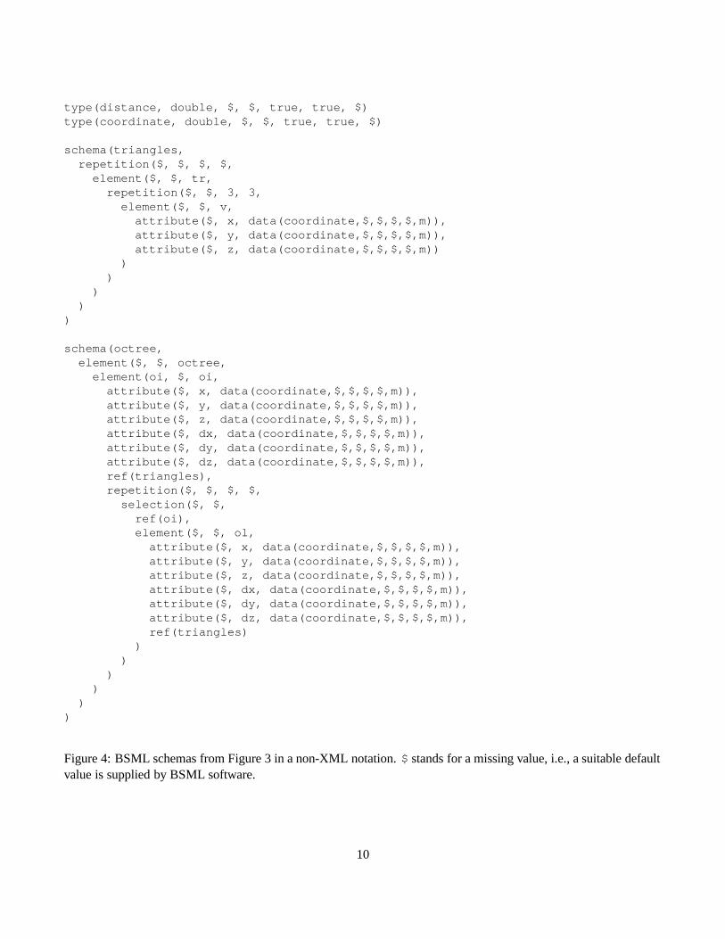
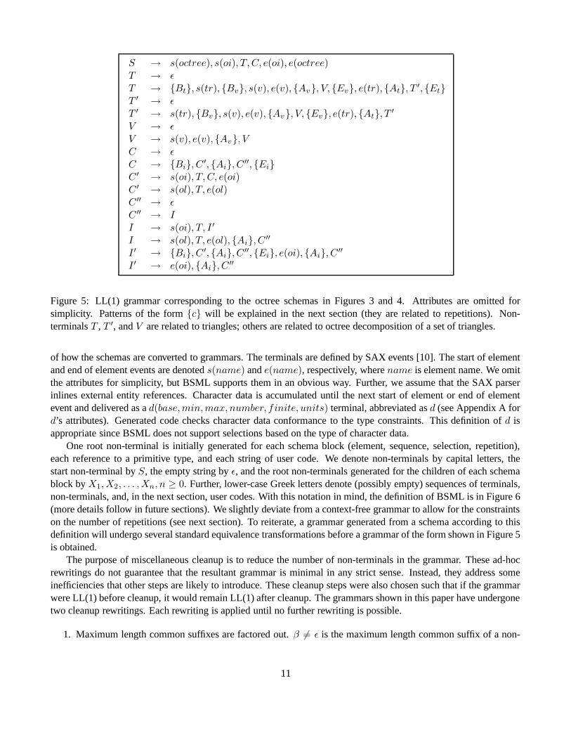
Let us start with an example. Figures 3 and 4 depict a (simplified) schema for an octree environment decompo-sition. (Fig. 3 describes it in XML notation while Fig. 4 uses a non-XML format that will be useful for describingsome functionalities of BSML). This is the most complex schema in S4W, not counting the schema for the schemalanguage itself. An octree consists of internal and leaf nodes that delimit groups of triangles. Recall from Section 1.1that this grouping is used to limit the intersection tests in ray tracing. The nested structure of an octree maps nicelyinto an XML tree. Since many components work with lists of triangles, there is a separate schema for a list oftriangles. As the example shows, the features of BSML closely resemble those of other schema languages, such asRELAX NG. The only noticeable difference is the presence of units in the definitions of primitive types. Units willbe useful for certain types of conversions. Figure 5 shows an LL(1) grammar generated from the octree schema.This grammar is then annotated with binding code and used to generate a parser for octree data. The parser can belinked with a parallel ray tracer written in C.

The DTD for the current version of BSML is given in Appendix A. The schema language describes primitivetypes and schemas. There are four base primitive types: integer, string, (IEEE) double, and boolean. Users canderive their own primitive types by range restriction. User-derived types usually have domain-specific flavor, suchas coordinates and distances in the example above. We do not support more complicated primitive types, suchas dates and lists, because each PSE component treats them differently. Schemas consist of four building blocks:elements, sequences, selections, and repetitions. Strictly speaking, repetitions can be expressed as selections andsequences, but they are so common that they deserve special treatment. Derivation of schemas by restriction isnot supported, but derivation by extension can be implemented via inter-schema references. Mixed content is notsupported because it is only used for documentation. Instead, BSML supports a wildcard content type. The contentsof this type matches anything and is delivered to the component as a DOM tree [6]. We do not support referentialintegrity constraints because they can delay binding and thus break requirement 7. There is no explicit construct forinterleaves. In some ways, interleaves are handled by the conversion algorithm. In other words, BSML is a simpleschema language that incorporates most common features that are useful in a PSE.

Parser generation for a BSML schema follows the standard steps from compiler textbooks [3]:

1. convert the schema to an LL(1) grammar,

2. eliminate empty productions and self-derivations,

3. eliminate left recursion,

4. perform left factoring,

5. perform miscellaneous cleanup (described in detail below),

6. compute a predictive parsing table, and

7. generate parsing code from the table.

The only steps specific to this schema language are generating an LL(1) grammar (step 1) and miscellaneouscleanup (step 5). Since grammars have been in use for a long time, it is pertinent to define BSML semantics in terms

8

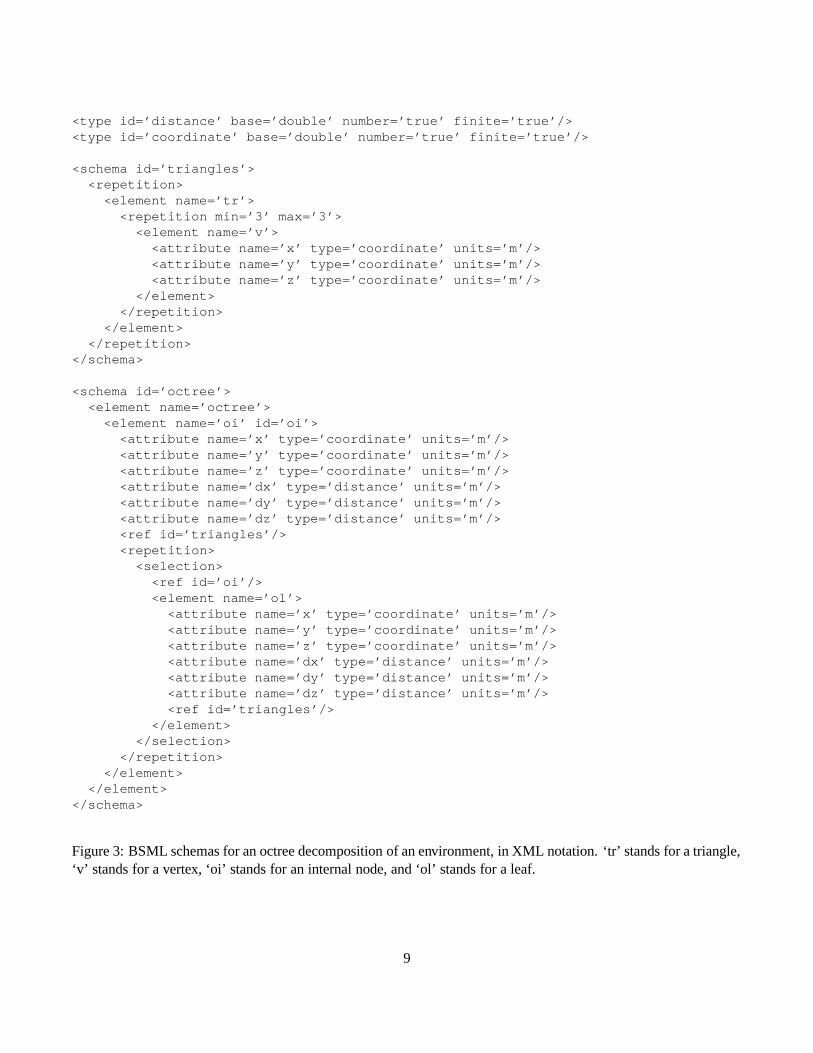
<type id=’distance’ base=’double’ number=’true’ finite=’true’/><type id=’coordinate’ base=’double’ number=’true’ finite=’true’/>

<schema id=’triangles’><repetition><element name=’tr’>

<repetition min=’3’ max=’3’><element name=’v’><attribute name=’x’ type=’coordinate’ units=’m’/><attribute name=’y’ type=’coordinate’ units=’m’/><attribute name=’z’ type=’coordinate’ units=’m’/>

</element></repetition>


</schema>

<schema id=’octree’><element name=’octree’><element name=’oi’ id=’oi’>

<attribute name=’x’ type=’coordinate’ units=’m’/><attribute name=’y’ type=’coordinate’ units=’m’/><attribute name=’z’ type=’coordinate’ units=’m’/><attribute name=’dx’ type=’distance’ units=’m’/><attribute name=’dy’ type=’distance’ units=’m’/><attribute name=’dz’ type=’distance’ units=’m’/><ref id=’triangles’/><repetition>

<selection><ref id=’oi’/><element name=’ol’>

<attribute name=’x’ type=’coordinate’ units=’m’/><attribute name=’y’ type=’coordinate’ units=’m’/><attribute name=’z’ type=’coordinate’ units=’m’/><attribute name=’dx’ type=’distance’ units=’m’/><attribute name=’dy’ type=’distance’ units=’m’/><attribute name=’dz’ type=’distance’ units=’m’/><ref id=’triangles’/>

</element></selection>

</repetition></element>

</element></schema>

Figure 3: BSML schemas for an octree decomposition of an environment, in XML notation. ‘tr’ stands for a triangle,‘v’ stands for a vertex, ‘oi’ stands for an internal node, and ‘ol’ stands for a leaf.

9

type(distance, double, $, $, true, true, $)type(coordinate, double, $, $, true, true, $)

schema(triangles,repetition($, $, $, $,element($, $, tr,

repetition($, $, 3, 3,element($, $, v,attribute($, x, data(coordinate,$,$,$,$,m)),attribute($, y, data(coordinate,$,$,$,$,m)),attribute($, z, data(coordinate,$,$,$,$,m))

))

))

)

schema(octree,element($, $, octree,element(oi, $, oi,

attribute($, x, data(coordinate,$,$,$,$,m)),attribute($, y, data(coordinate,$,$,$,$,m)),attribute($, z, data(coordinate,$,$,$,$,m)),attribute($, dx, data(coordinate,$,$,$,$,m)),attribute($, dy, data(coordinate,$,$,$,$,m)),attribute($, dz, data(coordinate,$,$,$,$,m)),ref(triangles),repetition($, $, $, $,

selection($, $,ref(oi),element($, $, ol,

attribute($, x, data(coordinate,$,$,$,$,m)),attribute($, y, data(coordinate,$,$,$,$,m)),attribute($, z, data(coordinate,$,$,$,$,m)),attribute($, dx, data(coordinate,$,$,$,$,m)),attribute($, dy, data(coordinate,$,$,$,$,m)),attribute($, dz, data(coordinate,$,$,$,$,m)),ref(triangles)

))

))

))

Figure 4: BSML schemas from Figure 3 in a non-XML notation. $ stands for a missing value, i.e., a suitable defaultvalue is supplied by BSML software.

10

S → s(octree), s(oi), T, C, e(oi), e(octree)T → εT → {Bt}, s(tr), {Bv}, s(v), e(v), {Av}, V, {Ev}, e(tr), {At}, T ′, {Et}T ′ → εT ′ → s(tr), {Bv}, s(v), e(v), {Av}, V, {Ev}, e(tr), {At}, T ′

V → εV → s(v), e(v), {Av}, VC → εC → {Bi}, C ′, {Ai}, C ′′, {Ei}C ′ → s(oi), T, C, e(oi)C ′ → s(ol), T, e(ol)C ′′ → εC ′′ → II → s(oi), T, I ′

I → s(ol), T, e(ol), {Ai}, C ′′

I ′ → {Bi}, C ′, {Ai}, C ′′, {Ei}, e(oi), {Ai}, C ′′

I ′ → e(oi), {Ai}, C ′′

Figure 5: LL(1) grammar corresponding to the octree schemas in Figures 3 and 4. Attributes are omitted forsimplicity. Patterns of the form {c} will be explained in the next section (they are related to repetitions). Non-terminals T , T ′, and V are related to triangles; others are related to octree decomposition of a set of triangles.

of how the schemas are converted to grammars. The terminals are defined by SAX events [10]. The start of elementand end of element events are denoted s(name) and e(name), respectively, where name is element name. We omitthe attributes for simplicity, but BSML supports them in an obvious way. Further, we assume that the SAX parserinlines external entity references. Character data is accumulated until the next start of element or end of elementevent and delivered as a d(base,min,max, number, finite, units) terminal, abbreviated as d (see Appendix A ford’s attributes). Generated code checks character data conformance to the type constraints. This definition of d isappropriate since BSML does not support selections based on the type of character data.

One root non-terminal is initially generated for each schema block (element, sequence, selection, repetition),each reference to a primitive type, and each string of user code. We denote non-terminals by capital letters, thestart non-terminal by S, the empty string by ε, and the root non-terminals generated for the children of each schemablock by X1, X2, . . . , Xn, n ≥ 0. Further, lower-case Greek letters denote (possibly empty) sequences of terminals,non-terminals, and, in the next section, user codes. With this notation in mind, the definition of BSML is in Figure 6(more details follow in future sections). We slightly deviate from a context-free grammar to allow for the constraintson the number of repetitions (see next section). To reiterate, a grammar generated from a schema according to thisdefinition will undergo several standard equivalence transformations before a grammar of the form shown in Figure 5is obtained.

The purpose of miscellaneous cleanup is to reduce the number of non-terminals in the grammar. These ad-hocrewritings do not guarantee that the resultant grammar is minimal in any strict sense. Instead, they address someinefficiencies that other steps are likely to introduce. These cleanup steps were also chosen such that if the grammarwere LL(1) before cleanup, it would remain LL(1) after cleanup. The grammars shown in this paper have undergonetwo cleanup rewritings. Each rewriting is applied until no further rewriting is possible.

1. Maximum length common suffixes are factored out. β 6= ε is the maximum length common suffix of a non-

11

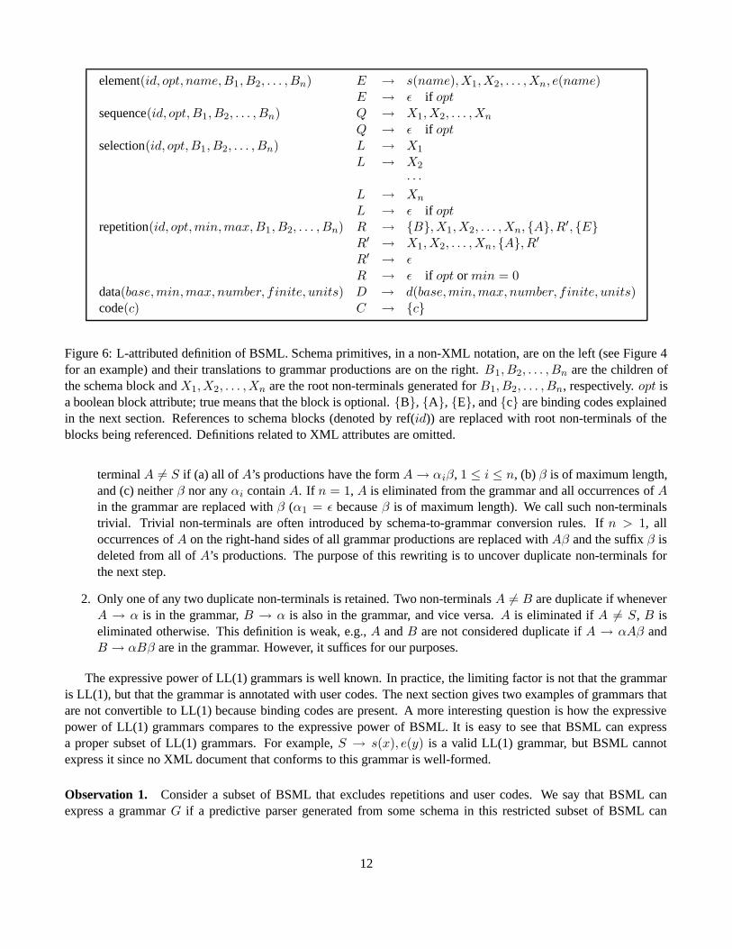
element(id, opt, name,B1, B2, . . . , Bn) E → s(name), X1, X2, . . . , Xn, e(name)E → ε if opt

sequence(id, opt,B1, B2, . . . , Bn) Q → X1, X2, . . . , Xn

Q → ε if optselection(id, opt,B1, B2, . . . , Bn) L → X1

L → X2

· · ·L → Xn

L → ε if optrepetition(id, opt,min,max,B1, B2, . . . , Bn) R → {B}, X1, X2, . . . , Xn, {A}, R′, {E}

R′ → X1, X2, . . . , Xn, {A}, R′

R′ → εR → ε if opt or min = 0

data(base,min,max, number, finite, units) D → d(base,min,max, number, finite, units)code(c) C → {c}

Figure 6: L-attributed definition of BSML. Schema primitives, in a non-XML notation, are on the left (see Figure 4for an example) and their translations to grammar productions are on the right. B1, B2, . . . , Bn are the children ofthe schema block and X1, X2, . . . , Xn are the root non-terminals generated for B1, B2, . . . , Bn, respectively. opt isa boolean block attribute; true means that the block is optional. {B}, {A}, {E}, and {c} are binding codes explainedin the next section. References to schema blocks (denoted by ref(id)) are replaced with root non-terminals of theblocks being referenced. Definitions related to XML attributes are omitted.

terminal A 6= S if (a) all of A’s productions have the form A → αiβ, 1 ≤ i ≤ n, (b) β is of maximum length,and (c) neither β nor any αi contain A. If n = 1, A is eliminated from the grammar and all occurrences of Ain the grammar are replaced with β (α1 = ε because β is of maximum length). We call such non-terminalstrivial. Trivial non-terminals are often introduced by schema-to-grammar conversion rules. If n > 1, alloccurrences of A on the right-hand sides of all grammar productions are replaced with Aβ and the suffix β isdeleted from all of A’s productions. The purpose of this rewriting is to uncover duplicate non-terminals forthe next step.

2. Only one of any two duplicate non-terminals is retained. Two non-terminals A 6= B are duplicate if wheneverA → α is in the grammar, B → α is also in the grammar, and vice versa. A is eliminated if A 6= S, B iseliminated otherwise. This definition is weak, e.g., A and B are not considered duplicate if A → αAβ andB → αBβ are in the grammar. However, it suffices for our purposes.

The expressive power of LL(1) grammars is well known. In practice, the limiting factor is not that the grammaris LL(1), but that the grammar is annotated with user codes. The next section gives two examples of grammars thatare not convertible to LL(1) because binding codes are present. A more interesting question is how the expressivepower of LL(1) grammars compares to the expressive power of BSML. It is easy to see that BSML can expressa proper subset of LL(1) grammars. For example, S → s(x), e(y) is a valid LL(1) grammar, but BSML cannotexpress it since no XML document that conforms to this grammar is well-formed.

Observation 1. Consider a subset of BSML that excludes repetitions and user codes. We say that BSML canexpress a grammar G if a predictive parser generated from some schema in this restricted subset of BSML can

12

recognize precisely the language L(G). Clearly, BSML cannot express any grammar G that is not LL(1) (by con-struction of the predictive parser). Further, BSML cannot express an LL(1) grammar G unless:

1. if d1 and d2 are data terminals in G, then ∀α, β : S ;+ α, d1, d2, β (data is atomic),

2. if d is a data terminal and S ⇒+ α, d, β is a derivation in G, then

∀x, γ :(

[β ;∗ s(x), γ] and [(β ⇒∗ e(x), γ) implies (∀y, θ : α ;

∗ θ, e(y))])

(no mixed contents), and

3. if s(x) is a start of element terminal, g is ε or a data terminal, and S ⇒+ α, s(x), β is a derivation in G, then(

[β ;∗ g] and [(y 6= x) implies (∀γ : β ;

∗ g, e(y), γ)])

; similarly, if e(y) is an end of element terminal and

S ⇒+ α, e(x), β is a derivation in G, then(

[α ;∗ g] and [(x 6= y) implies (∀θ : α ;

∗ θ, s(x), g)])

(proper

nesting of elements). 2

The first two restrictions are specific to BSML and easy to relax. However, the last restriction is inherent in anyXML schema language. A good schema language cannot describe documents that are not well-formed. These arethe necessary conditions, but it is not clear whether or not they are sufficient. We define schemas in terms of theschema language, not in terms of LL(1) grammars, so converting from grammars to schemas is not considered inthis paper.

This section provided an overview of BSML features and defined BSML in terms of an ‘almost context-free’grammar. We outlined automatic generation of predictive parsers that validate XML documents. Further, we haveshown that the descriptive power of BSML is strictly less than that of an LL(1) grammar where the terminals areSAX events. The next section extends validation to perform binding.

5 Binding

Binding is a way to integrate semistructured data with languages that were not designed to handle it (requirement 1).Binding can take several forms, depending on the language. For FORTRAN and C, binding usually means assigningvalues to language variables and calling user-defined code to process these values (procedural binding). It can alsomean writing the data out in a format understood by the component (format conversion). For Matlab and SQL,binding entails generating a script that contains embedded data and processing this script by an interpreter (codegeneration). The last two kinds of binding can be thought of as XSLT-like transformations.

We implement all three kinds of binding by L-attributed definitions. The schema language is extended byallowing user code to be injected in the schema. Schema languages that provide binding are called binding schemamarkup languages. This section describes bindings in BSML and gives an example of their use. Further, we showhow arbitrary binding codes limit the set of schemas supported by BSML. Predictive parsing cannot handle commonprefixes in alternative productions, so standard techniques are used to eliminate such common prefixes. We showthat these techniques break when the common prefixes contain binding codes. This limitation is rarely an issue andthe problems it causes can be remedied by simple modifications to the schema.

Let c denote an arbitrary string of code. Matching {c} means executing code c while consuming no input tokens.No assumptions are made about the nature of c. In particular, c can (and usually does) produce side effects, soA → {c1}, {c2} and A → {c2}, {c1} can yield different results. A syntax-directed definition is a context-freegrammar extended by allowing {cj} on the right-hand sides of productions. For a syntax-directed definition to beuseful in binding, cj must contain references to parts of the document being parsed. We denote such references by%x, where x is the id or the name of some element or attribute. When x refers to an attribute or an element of someprimitive type, %x is a value of the attribute or the data contents of the element. The type of %x is determined by thecorresponding primitive type. When x refers to an element of a wildcard type, %x is a DOM tree constructed from

13

all descendants of x, including itself. This feature can be used for XHTML [21] documentation. The set of attributes(elements) that are available to code c depends on the placement of c in the syntax-directed definition and the parsingstrategy. A syntax-directed definition is L-attributed if, for any derivation S ⇒+ α{c}β, any x referenced in c isdefined in all derivations of α. That is, all attributes (elements) must be defined in a left-to-right scan before they arereferenced. L-attributed definitions are easy to implement with an LL(1) parser, but they restrict the set of grammarsreducible to LL(1). Luckily, these restrictions are not important in practice.

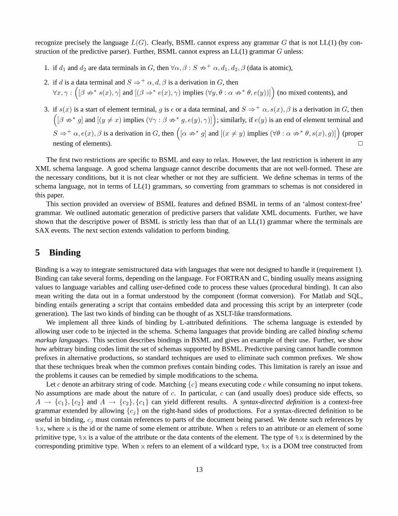
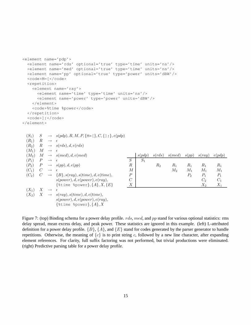
Figure 7 gives an example binding schema for a PDP (see Section 1.1) and Figure 8 shows how a parser generatedfrom this schema converts a PDP encoded in XML to a Matlab script. This script will then be executed by anexecution manager (see Section 7). The same schema, with different binding code, can convert an XML file toa number of SQL INSERT statements that record the data in a relational database. The semantics of user codesare not limited to printing, so a FORTRAN version of this binding can store the PDP in an array to be processedlater. In other words, BSML bindings are compatible with any execution environment that processes streams of data(requirement 7). We use the same approach to convert semistructured data to relational data, Matlab scripts, and Cstructures.

The {B}, {A}, and {E} codes in Figure 7 are generated for repetitions. They are not necessary for this example,but are required to enforce that each triangle has three vertices in the previous example. {B} (begin repetition)initializes the repetition count to zero. Each repetition has its own stack of counts. {A} (append) ensures that themaximum allowed number of repetitions is not exceeded. {E} (end) checks the minimum number of repetitions.Thus, even simple validation (without binding) is implemented in terms of an L-attributed definition, not just anLL(1) grammar.

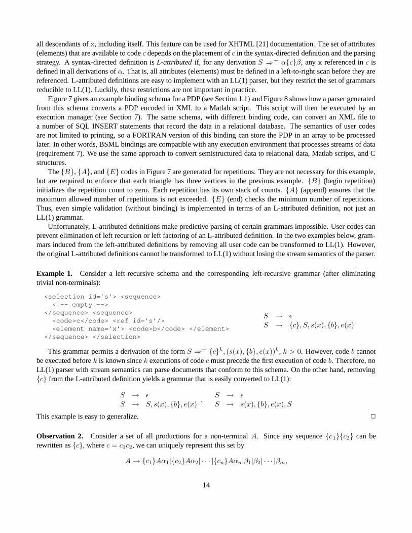
Unfortunately, L-attributed definitions make predictive parsing of certain grammars impossible. User codes canprevent elimination of left recursion or left factoring of an L-attributed definition. In the two examples below, gram-mars induced from the left-attributed definitions by removing all user code can be transformed to LL(1). However,the original L-attributed definitions cannot be transformed to LL(1) without losing the stream semantics of the parser.

Example 1. Consider a left-recursive schema and the corresponding left-recursive grammar (after eliminatingtrivial non-terminals):

<selection id=’s’> <sequence>

</sequence> <sequence><code>c</code> <ref id=’s’/><element name=’x’> <code>b</code> </element>

</sequence> </selection>

S → εS → {c}, S, s(x), {b}, e(x)

This grammar permits a derivation of the form S ⇒+ {c}k, (s(x), {b}, e(x))k , k > 0. However, code b cannotbe executed before k is known since k executions of code c must precede the first execution of code b. Therefore, noLL(1) parser with stream semantics can parse documents that conform to this schema. On the other hand, removing{c} from the L-attributed definition yields a grammar that is easily converted to LL(1):

S → εS → S, s(x), {b}, e(x)

,S → εS → s(x), {b}, e(x), S

This example is easy to generalize. 2

Observation 2. Consider a set of all productions for a non-terminal A. Since any sequence {c1}{c2} can berewritten as {c}, where c = c1c2, we can uniquely represent this set by

A → {c1}Aα1|{c2}Aα2| · · · |{cn}Aαn|β1|β2| · · · |βm,

14

<element name=’pdp’><element name=’rds’ optional=’true’ type=’time’ units=’ns’/><element name=’med’ optional=’true’ type=’time’ units=’ns’/><element name=’pp’ optional=’true’ type=’power’ units=’dBW’/><code>M=[</code><repetition><element name=’ray’>

<element name=’time’ type=’time’ units=’ns’/><element name=’power’ type=’power’ units=’dBW’/>

</element><code>%time %power</code>

</repetition><code>];</code>

</element>

(S1) S → s(pdp), R, M, P, {M=[}, C, {];}, e(pdp)(R1) R → ε(R2) R → s(rds), d, e(rds)(M1) M → ε(M2) M → s(med), d, e(med)(P1) P → ε(P2) P → s(pp), d, e(pp)(C1) C → ε(C2) C → {B}, s(ray), s(time), d, e(time),

s(power), d, e(power), e(ray),{%time %power}, {A}, X, {E}

(X1) X → ε(X2) X → s(ray), s(time), d, e(time),

s(power), d, e(power), e(ray),{%time %power}, {A}, X

s(pdp) s(rds) s(med) s(pp) s(ray) e(pdp)S S1

R R2 R1 R1 R1 R1

M M2 M1 M1 M1

P P2 P1 P1

C C2 C1

X X2 X1

Figure 7: (top) Binding schema for a power delay profile. rds, med, and pp stand for various optional statistics: rmsdelay spread, mean excess delay, and peak power. These statistics are ignored in this example. (left) L-attributeddefinition for a power delay profile. {B}, {A}, and {E} stand for codes generated by the parser generator to handlerepetitions. Otherwise, the meaning of {c} is to print string c, followed by a new line character, after expandingelement references. For clarity, full suffix factoring was not performed, but trivial productions were eliminated.(right) Predictive parsing table for a power delay profile.

15

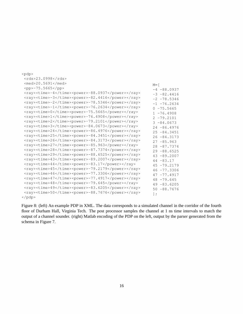
<pdp><rds>23.0998</rds><med>20.5691</med><pp>-75.5665</pp><ray><time>-4</time><power>-88.0937</power></ray><ray><time>-3</time><power>-82.4416</power></ray><ray><time>-2</time><power>-78.5346</power></ray><ray><time>-1</time><power>-76.2634</power></ray><ray><time>0</time><power>-75.5665</power></ray><ray><time>1</time><power>-76.4908</power></ray><ray><time>2</time><power>-79.2101</power></ray><ray><time>3</time><power>-84.0673</power></ray><ray><time>24</time><power>-86.4976</power></ray><ray><time>25</time><power>-84.3451</power></ray><ray><time>26</time><power>-84.3173</power></ray><ray><time>27</time><power>-85.963</power></ray><ray><time>28</time><power>-87.7374</power></ray><ray><time>29</time><power>-88.6525</power></ray><ray><time>43</time><power>-89.2007</power></ray><ray><time>44</time><power>-83.17</power></ray><ray><time>45</time><power>-79.2179</power></ray><ray><time>46</time><power>-77.3306</power></ray><ray><time>47</time><power>-77.4917</power></ray><ray><time>48</time><power>-79.645</power></ray><ray><time>49</time><power>-83.6205</power></ray><ray><time>50</time><power>-88.7676</power></ray>

</pdp>

M=[-4 -88.0937-3 -82.4416-2 -78.5346-1 -76.26340 -75.56651 -76.49082 -79.21013 -84.067324 -86.497625 -84.345126 -84.317327 -85.96328 -87.737429 -88.652543 -89.200744 -83.1745 -79.217946 -77.330647 -77.491748 -79.64549 -83.620550 -88.7676];

Figure 8: (left) An example PDP in XML. The data corresponds to a simulated channel in the corridor of the fourthfloor of Durham Hall, Virginia Tech. The post processor samples the channel at 1 ns time intervals to match theoutput of a channel sounder. (right) Matlab encoding of the PDP on the left, output by the parser generated from theschema in Figure 7.

16

where no βj , 1 ≤ j ≤ m, has a prefix {d}A. Immediate left recursion can be eliminated from this productionwithout delaying user code execution if and only if

1. c1 = c2 = · · · = cn = ε (no user code to the left) or

2.(

[(βj ⇒∗ γ{d}θ, 1 ≤ j ≤ m) or (αi ⇒∗ γ{d}θ, 1 ≤ i ≤ n)] implies (d = ε))

(no user code to the right)

and (c1 = c2 = · · · = cn) (same user code to the left).

In all other cases, execution of user code must be delayed until the last αi is matched. 2

Consider a derivation of A that is no longer left-recursive (i.e., does not have a prefix of {d}A). All suchderivations can be written as

A ⇒+ {ci1}, {ci2}, . . . , {cik}, βj , αik , . . . , αi2 , αi1 ,

where βj , 1 ≤ j ≤ m, stops left recursion after (at least) k + 1 steps and 1 ≤ i1, i2, . . . , ik ≤ n represent thechoices for αi in the derivation. Suppose βj ⇒∗ γ{d}θ or αi ⇒∗ γ{d}θ. The sequence of codes ci1 , ci2 , . . . , cik

must be executed before code d, but the LL(1) parser will only determine this sequence after it has parsed all ofβj , αik , . . . , αi2 , αi1 . Thus, eliminating left recursion entails delaying user code execution in all but the trivial casesmentioned above.

Example 2. Left factoring of L-attributed definitions poses similar problems. Consider the following schema andL-attributed definition (a more realistic version of this example would have a repetition in place of the x element):

<selection> <sequence><code>c</code><element name=’x’/><element name=’y’/>

</sequence> <sequence><code>d</code><element name=’x’/><element name=’z’/>

</sequence> </selection>

S → {c}, s(x), e(x), s(y), e(y)S → {d}, s(x), e(x), s(z), e(z)

The decision about whether to execute code c or d cannot be made until s(y) or s(z) is processed. However, removinguser codes makes this L-attributed definition easy to refactor. Again, we can show a more general condition. 2

Observation 3. Consider a set of all productions for a non-terminal A written as

A → α1β1|α2β2| · · · |αnβn|γ1|γ2| · · · |γm,

such that α′1 = α′

2 = · · · = α′n = α 6= ε (α′ denotes α with all user code removed) and α is not a prefix of any

γ′1, γ

′2, . . . , γ

′m. Let the length of α be maximum and the lengths of αi, 1 ≤ i ≤ n, be minimum subject to n ≥ 2, in

which case this representation of A is unique. A can be left-factored without delaying execution of user code if andonly if

1. no rewriting of A in the above form exists (no two definitions of A share the same prefix, less user codes), or

2. α1 = α2 = · · · = αn (same codes to the left) and A → γ1|γ2| · · · |γm can be left-factored. 2

To summarize, we implement bindings in terms of L-attributed definitions from parsing theory. These bindingswork well in practice, but, in theory, annotating a schema that can be rewritten in LL(1) form can make it no longerrewritable in LL(1) form. This difficulty is inherent in L-attributed definitions. We currently assume that the useris responsible for resolving such conflicts. In practice, schemas for PSE data rarely require complicated grammars.Repetitions take care of most of the recursive schema definitions. To make LL(1) parsing possible, troublesomecontent can be simply enclosed in an extra XML element, whose start and end tags disambiguate the transitions ofthe LL(1) parser.

17

6 Conversion

Conversion is the cornerstone of a system’s ability to handle changes and interface mismatches. Conversion in aPSE helps to retain historical data and facilitates inclusion of new components. We use change detection principlesfrom [11], with a few important differences. First, our goal is not merely to detect changes, but to make PSE com-ponents work despite the changes. Second, we detect changes in the schema, not in the data. The PSE environmentmust guarantee that the data is in the right format for the component. The job of the component is to process any datainstance that conforms to the right format. Last, change detection and conversion are local to the extent possible.Locality is a virtue not only because it allows for stream processing, but also because it limits sporadic conversionsbetween unrelated entities.

Similarly to the two previous sections, this section starts with a comprehensive example. Then, we describethe core of the conversion algorithm and outline its limitations. Finally, we extend the initial algorithm to handlecontent replacements: unit conversion and user-defined conversion filters. At this point, it should not come as asurprise to the reader that most of the technical limitations of conversion are due to binding codes, not to the natureof the schema language. Therefore, the tedious details of handling binding codes are omitted. The emphasis is onnon-technical limitations. What forms of semantic conversions can be ‘syntactized’ in a schema language? Whendoes such ‘syntactization’ back fire and produce undesired outcomes?

The functional statement of the conversion problem can be given as follows. Given the actual schema Sa andthe required schema Sr, replace binding codes in Sa with binding codes in Sr and conversion codes to obtain theconversion schema Sc. Sc must describe precisely the documents described by Sa, but perform the same bindingsas Sr.

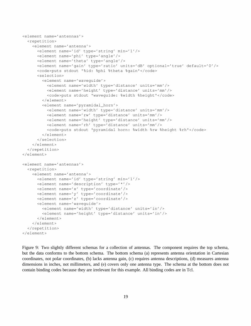
Example 3. Figure 9 depicts two slightly different schemas for antenna descriptions in S4W. The schema at thebottom (actual schema) was our first attempt at defining a data format for antenna descriptions. This version sup-ported only one antenna type and exhibited several inadequate representation choices. E.g., polar coordinates shouldhave been used instead of Cartesian coordinates because antenna designers prefer to work in the polar coordinatesystem. Antenna gain was not considered in the first version because its effect is the same as that of changingtransmitter power. However, this seemingly unnecessary parameter should have been included because it results ina more direct correspondence of simulation input to a physical system.

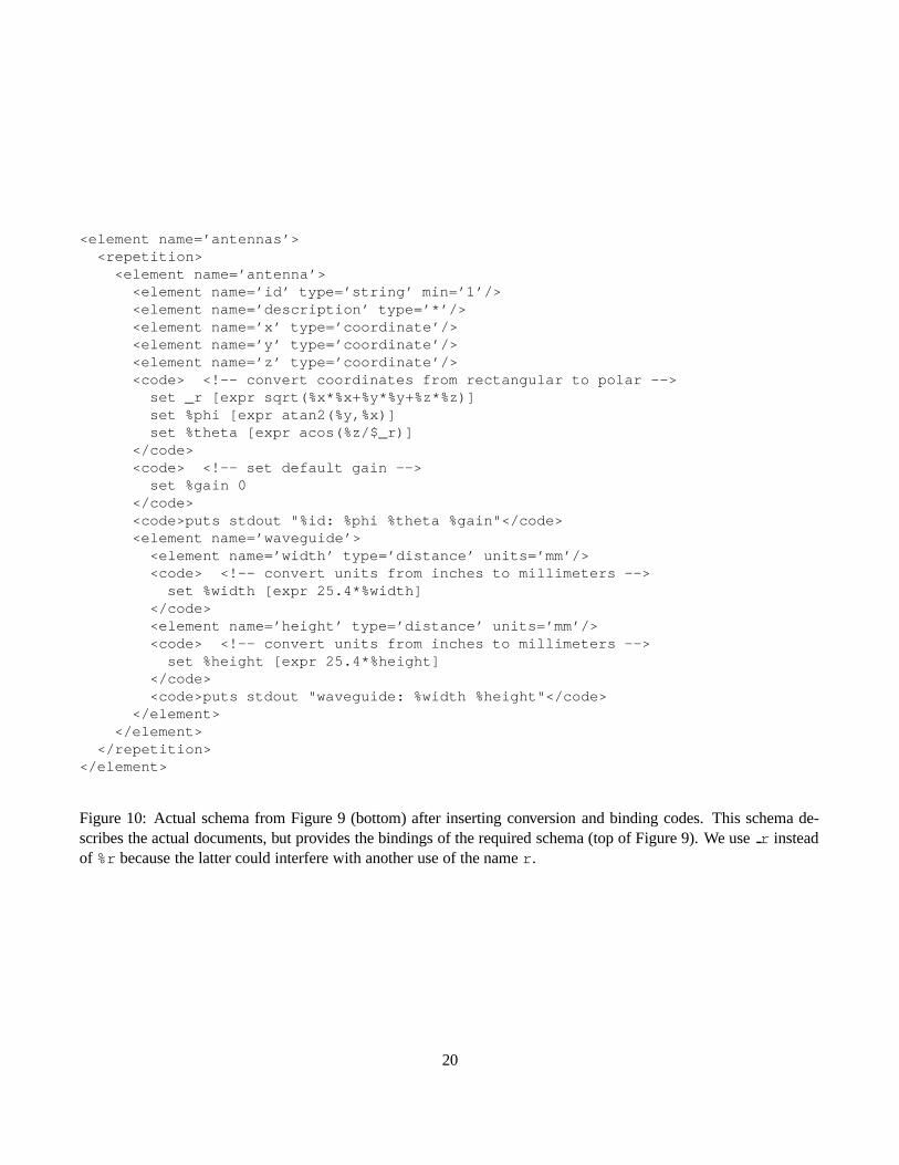
The schema at the top of Fig. 9 (required schema) improves upon the actual schema in several ways. It betteradheres to common practices and supports more antenna types. However, this schema is different from the actualschema, while compatibility with old data needs to be retained (requirement 2). Figure 10 illustrates how additionof conversion and binding codes to the actual schema solves the compatibility problem. A parser generated from theconversion schema in Figure 10 will recognize the actual data and provide the required binding. 2

Following [11], the basic assumption of the conversion algorithm is that the actual schema Sa can be converted tothe required schema Sr by some sequence of ‘standard’ edits. This sequence of edits is called an edit script. Oncethe possible types of edits are defined (what we can call a ‘conversion library’), the job of the conversion algorithmis to (a) find an edit script that transforms the actual schema Sa to the required schema Sr and (b) express thisedit script as data transformations, not schema transformations. In other words, the conversion algorithm looks for asystematic procedure that converts actual data instances that conform to Sa to the required format Sr. This procedureis expressed as a conversion schema Sc that has the structure of Sa, but binding codes from Sr and the conversionlibrary. Sc is then used to generate a parser that parses data instances conforming to Sa and acts as if it parsed datainstances conforming to Sr.

Our conversion algorithm supports four kinds of schema edits:

1. generalization,

18

<element name=’antennas’><repetition><element name=’antenna’>

<element name=’id’ type=’string’ min=’1’/><element name=’phi’ type=’angle’/><element name=’theta’ type=’angle’/><element name=’gain’ type=’ratio’ units=’dB’ optional=’true’ default=’0’/><code>puts stdout "%id: %phi %theta %gain"</code><selection>

<element name=’waveguide’><element name=’width’ type=’distance’ units=’mm’/><element name=’height’ type=’distance’ units=’mm’/><code>puts stdout "waveguide: %width %height"</code>

</element><element name=’pyramidal_horn’><element name=’width’ type=’distance’ units=’mm’/><element name=’rw’ type=’distance’ units=’mm’/><element name=’height’ type=’distance’ units=’mm’/><element name=’rh’ type=’distance’ units=’mm’/><code>puts stdout "pyramidal horn: %width %rw %height %rh"</code>

</element></selection>


</element>


<element name=’id’ type=’string’ min=’1’/><element name=’description’ type=’*’/><element name=’x’ type=’coordinate’/><element name=’y’ type=’coordinate’/><element name=’z’ type=’coordinate’/><element name=’waveguide’>

<element name=’width’ type=’distance’ units=’in’/><element name=’height’ type=’distance’ units=’in’/>

</element></element>


Figure 9: Two slightly different schemas for a collection of antennas. The component requires the top schema,but the data conforms to the bottom schema. The bottom schema (a) represents antenna orientation in Cartesiancoordinates, not polar coordinates, (b) lacks antenna gain, (c) requires antenna descriptions, (d) measures antennadimensions in inches, not millimeters, and (e) covers only one antenna type. The schema at the bottom does notcontain binding codes because they are irrelevant for this example. All binding codes are in Tcl.

19

<element name=’id’ type=’string’ min=’1’/><element name=’description’ type=’*’/><element name=’x’ type=’coordinate’/><element name=’y’ type=’coordinate’/><element name=’z’ type=’coordinate’/><code> 

set _r [expr sqrt(%x*%x+%y*%y+%z*%z)]set %phi [expr atan2(%y,%x)]set %theta [expr acos(%z/$_r)]

</code><code> 

set %gain 0</code><code>puts stdout "%id: %phi %theta %gain"</code><element name=’waveguide’>

<element name=’width’ type=’distance’ units=’mm’/><code> set %width [expr 25.4*%width]

</code><element name=’height’ type=’distance’ units=’mm’/><code> set %height [expr 25.4*%height]

</code><code>puts stdout "waveguide: %width %height"</code>



Figure 10: Actual schema from Figure 9 (bottom) after inserting conversion and binding codes. This schema de-scribes the actual documents, but provides the bindings of the required schema (top of Figure 9). We use r insteadof %r because the latter could interfere with another use of the name r.

20

Dr : data(basea,mina,maxa, numbera, f initea, unitsa) � data(baser,minr,maxr, numberr, f initer, unitsr)if basea = baser,mina ≥ minr,maxa ≤ maxr, numberr ⇒ numbera, f initer ⇒ finitea,unitsa = unitsr

E : element(ida, opta, namea, Ca1, Ca2, . . . , Can) � element(idr, optr, namer, Cr1, Cr2, . . . , Crm)if namea = namer, opta ⇒ optr, Qa(Ca1, Ca2, . . . , Can) � Qr(Cr1, Cr2, . . . , Crm)

Eg : Xa(ida, opta, . . .) � element(idr, optr, namer, Cr1, Cr2, . . . , Crm)if opta ⇒ optr, Qa(Xa(ida, opta, . . .)) � Qr(Cr1, Cr2, . . . , Crm)

Er : element(ida, opta, namea, Ca1, Ca2, . . . , Can) � Xr(idr, optr, . . .)if opta ⇒ optr, Qa(Ca1, Ca2, . . . , Can) � Xr(idr, optr, . . .)

P : sequence(ida, opta, Ca1, Ca2, . . . , Can) � sequence(idr, optr, Cr1, Cr2, . . . , Crm)if opta ⇒ optr, Qa(Ca1, Ca2, . . . , Can) � Qr(Cr1, Cr2, . . . , Crm)

Pg : Xa(ida, opta, . . .) � sequence(idr, optr, Cr1, Cr2, . . . , Crm)if opta ⇒ optr, Qa(Xa(ida, opta, . . .)) � Qr(Cr1, Cr2, . . . , Crm)

Pr : sequence(ida, opta, Ca1, Ca2, . . . , Can) � Xr(idr, optr, . . .)if opta ⇒ optr, Qa(Ca1, Ca2, . . . , Can) � Xr(idr, optr, . . .)

C : selection(ida, opta, Ca1, Ca2, . . . , Can) � selection(idr, optr, Cr1, Cr2, . . . , Crm)if opta ⇒ optr,∀Cai : (∃!Crj : Cai � Crj)

Cg : Xa(ida, opta, . . .) � selection(idr, optr, Cr1, Cr2, . . . , Crm)if opta ⇒ optr, (∃!Crj : Xa(ida, opta, . . .) � Crj)

R : repetition(ida, opta,mina,maxa, Ca1, Ca2, . . . , Can) � repetition(idr, optr,minr,maxr, Cr1, Cr2, . . . , Crm)if mina ≥ minr,maxa ≤ maxr, opta ⇒ optr, Qa(Ca1, Ca2, . . . , Can) � Qr(Cr1, Cr2, . . . , Crm)

Rg : Xa(ida, opta, . . .) � repetition(idr, optr,minr,maxr, Cr1, Cr2, . . . , Crm)if minr ≤ 1,maxr ≥ 1, opta ⇒ optr, Qa(Xa(ida, opta, . . .)) � Qr(Cr1, Cr2, . . . , Crm)

F : ref(ida) � ref(idr)if Xa(ida, opta, . . .) � Xr(idr, optr, . . .)

Q : Qa(Ca1, Ca2, . . . , Can) � Qr(Cr1, Cr2, . . . , Crm)if ∀Crj(. . . , optrj , . . .) : [(∃!Cai : Cai � Crj) or (optrj)]

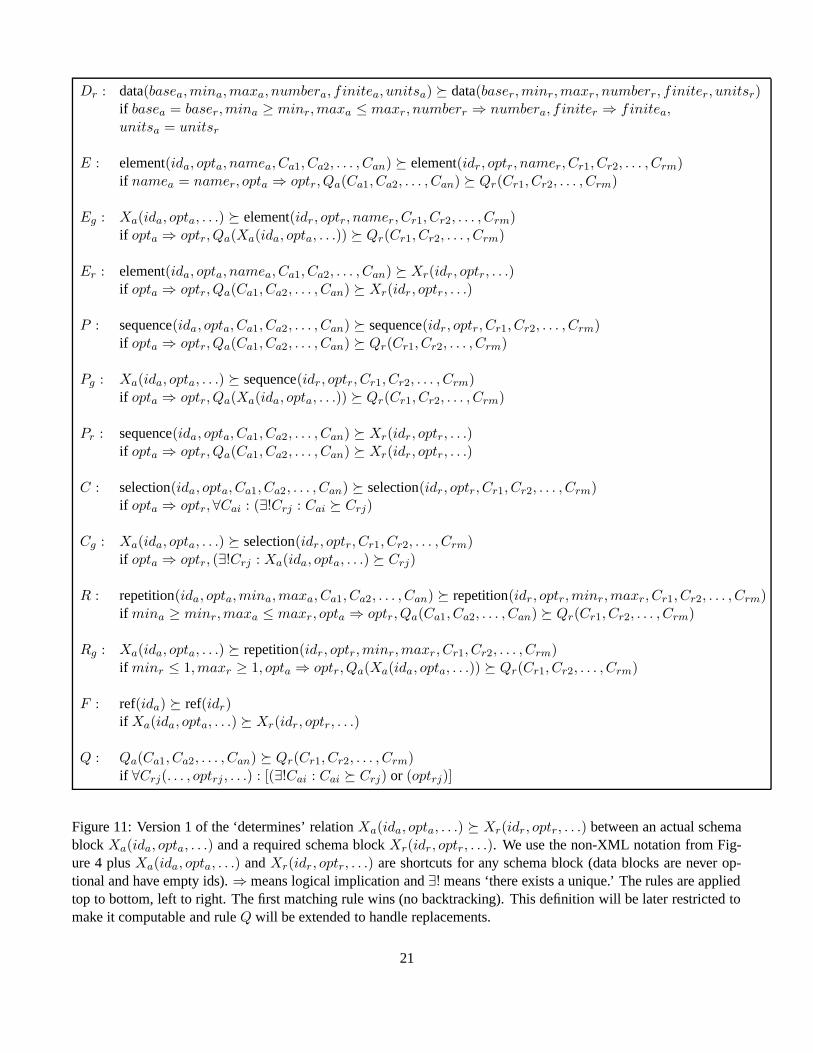
Figure 11: Version 1 of the ‘determines’ relation Xa(ida, opta, . . .) � Xr(idr, optr, . . .) between an actual schemablock Xa(ida, opta, . . .) and a required schema block Xr(idr, optr, . . .). We use the non-XML notation from Fig-ure 4 plus Xa(ida, opta, . . .) and Xr(idr, optr, . . .) are shortcuts for any schema block (data blocks are never op-tional and have empty ids). ⇒ means logical implication and ∃! means ‘there exists a unique.’ The rules are appliedtop to bottom, left to right. The first matching rule wins (no backtracking). This definition will be later restricted tomake it computable and rule Q will be extended to handle replacements.

21

2. restriction,

3. reordering, and

4. replacement.

We use these terms in reference to the required schema, e.g., ‘the required schema is a generalization of the actualschema.’ Generalization and restriction of schema trees are similar to insertions and deletions in sequence alignmentproblems. Reordering and replacement mostly retain their standard meaning, except we consider replacements ofsets of schema blocks, not individual schema blocks. We first reduce the problem of converting trees to an easierproblem of converting sequences (see Figure 11). Sequence conversion (rule Q) in this initial formulation performsall conversions but replacements. Then, we slightly restrict this definition to make it practical and generalize rule Qto accommodate replacements (unit conversion and user-defined conversion filters).

The conversion algorithm revolves around the ‘determines’ relation between schemas. Intuitively, an actualschema Sa should determine a required schema Sr if any document that conforms to Sa contains sufficient informa-tion to construct an ‘appropriate’ document that conforms to Sr. ‘Appropriate’ here is obviously a domain-specificnotion, and in the absence of a domain theory, there is no hard and fast measure of ‘appropriateness.’ Given twoslightly different schemas, only a domain expert can tell whether or not it is meaningful to attempt a conversionfrom one form to another. Therefore, our conversion rules should be viewed as heuristics that we have found tobe useful enough to be supported in a conversion library. They are neither sound nor complete in an algorithmicsense (because we do not have an objective, external, measure of ‘conversion correctness’). Instead, they representa tradeoff between soundness and completeness and should be carefully evaluated for use in a particular domain.With this disclaimer in mind, version 1 of the determines relation between Sa and Sr (Sa determines Sr; Sa � Sr)is defined in Figure 11. We will also find the notion of schema equivalence useful: we say that two schemas Sa andSr are equivalent if Sa � Sr and Sr � Sa.

The first rule (Dr) in Figure 11, for instance, says that a value of primitive type (‘data’) can be substituted foranother if they have the same base type, their ranges are compatible, and they have the same units. It ensures thatall primitive type constraints of Sr are met by Sa (restriction). Thus, Dr is simply a definition of type derivationby range restriction (the ‘r’ subscript in this and other rules stands for restriction; similarly, the ‘g’ subscript standsfor generalization). Rules E, P , and R state the obvious: two black boxes are compatible if they have compatiblewrappers (restriction) and compatible contents (any conversions). Rule C says that any choice in Sa must uniquelydetermine some choice in Sr (restriction). Rule Q enforces that every block in Sr is uniquely determined by someblock in Sa. This formulation of rule Q ignores extra blocks in Sa (restriction), permits optional elements in Sr tobe unmatched (generalization), and allows for contents reordering. Rule F deals with references. Only rules Dr,E, P , C , and R are sound. Rule F looks sound, but it makes the determines relation not computable. Rule Q isunsound primarily because it ignores ‘unnecessary’ blocks in Sa.

Rules Eg, Pg , Cg, and Rg handle generalizations across schema blocks of (possibly) different types. Theircounterparts Er and Pr handle symmetric restrictions (why is there no Cr or Rr?). Rule Cg was demonstrated inthe example above. It is a base case for rule C . Rule Cg states that one way to generalize a schema block is toenclose it in a selection, i.e., provide more choices in Sr than were available in Sa. This rule is sound. Rules Eg, Pg,and Rg have similar motivations, but they are unsound. Essentially, we assume that decorating any black box withany number of wrappers does not change the meaning of the black box (generalization). Similarly, we assume thatwrappers can be freely removed to expose the black box (restriction).

Consider a sequence of schemas that describes some physical system in progressively greater detail. Supposesome subsystem is described by a single parameter. Common practice is to allocate a single schema block to thissubsystem. What happens when a more detailed description of this subsystem is incorporated into the schema?Chances are, the original schema block allocated to the subsystem will be either (a) augmented with more con-tents (restriction part of rule Q) or (b) wrapped in another block. The generalization and restriction rules handle

22

case (b). However, blind application of these rules can lead to disaster because these rules disregard some semanticinformation. Examples will make these points clearer.

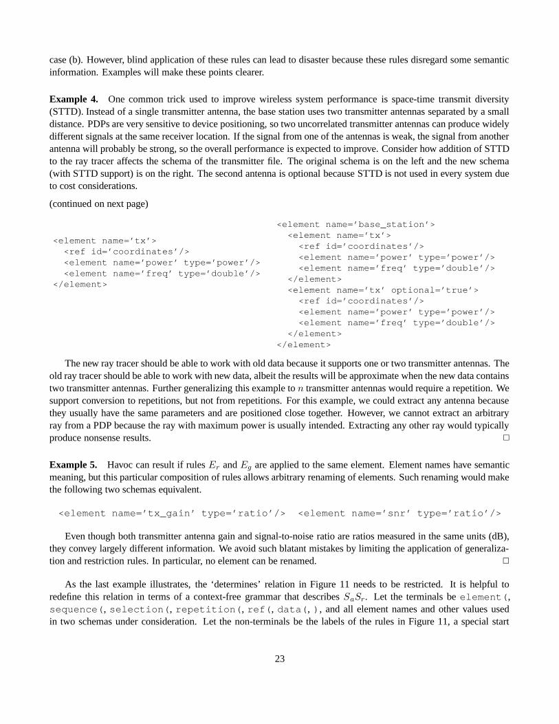
Example 4. One common trick used to improve wireless system performance is space-time transmit diversity(STTD). Instead of a single transmitter antenna, the base station uses two transmitter antennas separated by a smalldistance. PDPs are very sensitive to device positioning, so two uncorrelated transmitter antennas can produce widelydifferent signals at the same receiver location. If the signal from one of the antennas is weak, the signal from anotherantenna will probably be strong, so the overall performance is expected to improve. Consider how addition of STTDto the ray tracer affects the schema of the transmitter file. The original schema is on the left and the new schema(with STTD support) is on the right. The second antenna is optional because STTD is not used in every system dueto cost considerations.

(continued on next page)

<element name=’tx’><ref id=’coordinates’/><element name=’power’ type=’power’/><element name=’freq’ type=’double’/>

</element>

<element name=’base_station’><element name=’tx’>

<ref id=’coordinates’/><element name=’power’ type=’power’/><element name=’freq’ type=’double’/>

</element><element name=’tx’ optional=’true’>

<ref id=’coordinates’/><element name=’power’ type=’power’/><element name=’freq’ type=’double’/>


The new ray tracer should be able to work with old data because it supports one or two transmitter antennas. Theold ray tracer should be able to work with new data, albeit the results will be approximate when the new data containstwo transmitter antennas. Further generalizing this example to n transmitter antennas would require a repetition. Wesupport conversion to repetitions, but not from repetitions. For this example, we could extract any antenna becausethey usually have the same parameters and are positioned close together. However, we cannot extract an arbitraryray from a PDP because the ray with maximum power is usually intended. Extracting any other ray would typicallyproduce nonsense results. 2

Example 5. Havoc can result if rules Er and Eg are applied to the same element. Element names have semanticmeaning, but this particular composition of rules allows arbitrary renaming of elements. Such renaming would makethe following two schemas equivalent.

<element name=’tx_gain’ type=’ratio’/> <element name=’snr’ type=’ratio’/>

Even though both transmitter antenna gain and signal-to-noise ratio are ratios measured in the same units (dB),they convey largely different information. We avoid such blatant mistakes by limiting the application of generaliza-tion and restriction rules. In particular, no element can be renamed. 2

As the last example illustrates, the ‘determines’ relation in Figure 11 needs to be restricted. It is helpful toredefine this relation in terms of a context-free grammar that describes SaSr. Let the terminals be element(,sequence(, selection(, repetition(, ref(, data(, ), and all element names and other values usedin two schemas under consideration. Let the non-terminals be the labels of the rules in Figure 11, a special start

23

non-terminal A, and intermediate non-terminals introduced by the rules. We can formally define the necessaryrestrictions by limiting the shape of the parse tree for SaSr. Consider a path R1, R2, . . . , Rn, n > 0, from someinternal node R1 6= A to some internal node Rn 6= A, where all Ri, 1 ≤ i ≤ n, are rule labels. If R is the set ofrestriction rules and G is the set of generalization rules, we require that (Ri ∈ R) implies (Ri−1 /∈ G and Ri+1 /∈ G),i.e., restriction and generalization rules cannot be applied in sequence. This restriction of the parse tree disallowsrenaming of elements, but does not limit the number of wrappers around black boxes. Bounded determination dealswith the latter problem. We say that Sa k-determines Sr (Sa �k Sr) if no path R1, R2, . . . , Rn contains a substringof (possibly different) generalization (restriction) rules of length greater than k. We leave it up to the reader toappropriately restrict rule F (reference). These restrictions make the ‘determines’ relation computable and enforcelocality of conversions. As a side effect, we have shown that the problem of constructing a conversion schemaSc from the actual schema Sa and the required schema Sr can be reduced to validation and binding (parsing andtranslation). However, schema conversion need not work with streams of data, so a parser more powerful than apredictive parser should be used.

It remains to consider requirements 4 and 5: unit conversion and user-defined conversion filters (replacements).Let D be a set of all primitive types derived from double (recall that a primitive type is defined by the base type, therange of legal values, and a unit expression). Unit conversion, e.g., converting kg/m2 to lb/in2, is the simpler of thetwo replacements. Both actual and required unit expressions are converted to a canonical form (e.g., a fraction ofproducts of sums of CI units or dB) and then the conversion function is found. Unit conversions are functions of theform

U : Da → Dr,

where Da, Dr ∈ D are specific primitive types. User-defined conversion filters are functions of the form

H : Da1 × Da2 × · · · × Dan → Dr1 × Dr2 × · · · × Drm,

where n,m > 0 and all Dai, Drj ∈ D, 1 ≤ i ≤ n, 1 ≤ j ≤ m, are specific primitive types. Arithmetic operators andcommon mathematical functions are allowed in user-defined conversion filters. Each user-defined conversion filteris tagged with element names namea1, namea2, . . . , namean and namer1, namer2, . . . , namerm that determinewhen the filter applies. Such filters define rules of the form

(element($, $, namea1, Da1), element($, $, namea2, Da2), . . . , element($, $, namean, Dan)) �(element($, $, namer1, Dr1), element($, $, namer2, Dr2), . . . , element($, $, namerm, Drm)).

Both kinds of filters are compiled into codes such as shown in Figure 10. Rule Q is modified to take advantage ofreplacements. Basically, we are looking for (unique) partitions of the actual schema blocks Ca1, Ca2, . . . , Can andrequired schema blocks Cr1, Cr2, . . . , Crm such that each set of schema blocks in the required partition is determinedby some set of schema blocks in the actual partition. Determination can proceed through the rules in Figure 11, unitconversions, and user-defined conversion filters (if everything else fails, optional blocks in the required schema canremain unmatched).

The ultimate goal of the conversion algorithm is to find a meaningful edit script. However, this goal is impossibleto achieve without knowledge of the domain. What happens when several edit scripts exist, i.e., the problem offinding an edit script is ambiguous? Depending on the nature of the ambiguity, we can choose any edit script, theminimal (in some sense) edit script, or to refuse to perform conversion. The conversion algorithm described hereeither settles for some local minimum (e.g., rule E is preferred over rule Eg) or requires uniqueness of conversions(rules C , Cg , and most of rule Q). Ambiguity remains an open problem that is unlikely to be solved by a syntacticconversion algorithm. Following the principle of least user astonishment, we choose to reject most of ambiguousconversions.

Finally, let us consider how binding codes limit conversion. We omit formal treatment of the problem and limitthe discussion to an example. It is easy to see that conversion may require delaying binding code execution. Thisshould not be surprising since one kind of conversion is reordering.

24

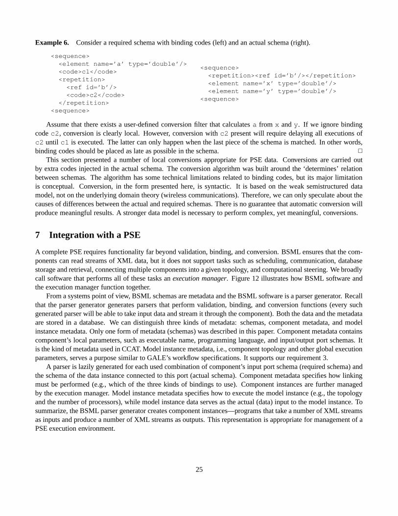
Example 6. Consider a required schema with binding codes (left) and an actual schema (right).

<sequence><element name=’a’ type=’double’/><code>c1</code><repetition>

<ref id=’b’/><code>c2</code>

</repetition><sequence>

<sequence><repetition><ref id=’b’/></repetition><element name=’x’ type=’double’/><element name=’y’ type=’double’/>

<sequence>

Assume that there exists a user-defined conversion filter that calculates a from x and y. If we ignore bindingcode c2, conversion is clearly local. However, conversion with c2 present will require delaying all executions ofc2 until c1 is executed. The latter can only happen when the last piece of the schema is matched. In other words,binding codes should be placed as late as possible in the schema. 2

This section presented a number of local conversions appropriate for PSE data. Conversions are carried outby extra codes injected in the actual schema. The conversion algorithm was built around the ‘determines’ relationbetween schemas. The algorithm has some technical limitations related to binding codes, but its major limitationis conceptual. Conversion, in the form presented here, is syntactic. It is based on the weak semistructured datamodel, not on the underlying domain theory (wireless communications). Therefore, we can only speculate about thecauses of differences between the actual and required schemas. There is no guarantee that automatic conversion willproduce meaningful results. A stronger data model is necessary to perform complex, yet meaningful, conversions.

7 Integration with a PSE

A complete PSE requires functionality far beyond validation, binding, and conversion. BSML ensures that the com-ponents can read streams of XML data, but it does not support tasks such as scheduling, communication, databasestorage and retrieval, connecting multiple components into a given topology, and computational steering. We broadlycall software that performs all of these tasks an execution manager. Figure 12 illustrates how BSML software andthe execution manager function together.

From a systems point of view, BSML schemas are metadata and the BSML software is a parser generator. Recallthat the parser generator generates parsers that perform validation, binding, and conversion functions (every suchgenerated parser will be able to take input data and stream it through the component). Both the data and the metadataare stored in a database. We can distinguish three kinds of metadata: schemas, component metadata, and modelinstance metadata. Only one form of metadata (schemas) was described in this paper. Component metadata containscomponent’s local parameters, such as executable name, programming language, and input/output port schemas. Itis the kind of metadata used in CCAT. Model instance metadata, i.e., component topology and other global executionparameters, serves a purpose similar to GALE’s workflow specifications. It supports our requirement 3.

A parser is lazily generated for each used combination of component’s input port schema (required schema) andthe schema of the data instance connected to this port (actual schema). Component metadata specifies how linkingmust be performed (e.g., which of the three kinds of bindings to use). Component instances are further managedby the execution manager. Model instance metadata specifies how to execute the model instance (e.g., the topologyand the number of processors), while model instance data serves as the actual (data) input to the model instance. Tosummarize, the BSML parser generator creates component instances—programs that take a number of XML streamsas inputs and produce a number of XML streams as outputs. This representation is appropriate for management of aPSE execution environment.

25

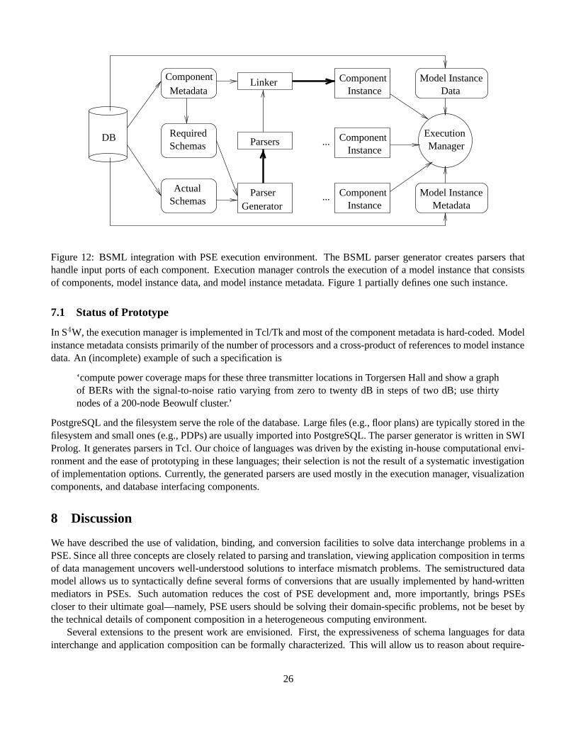
ExecutionManager

DB

ComponentInstance

Model InstanceMetadata

Model InstanceData

ComponentInstance

ComponentInstance

GeneratorParser

Parsers

LinkerComponentMetadata

ActualSchemas

RequiredSchemas ...

...

Figure 12: BSML integration with PSE execution environment. The BSML parser generator creates parsers thathandle input ports of each component. Execution manager controls the execution of a model instance that consistsof components, model instance data, and model instance metadata. Figure 1 partially defines one such instance.

7.1 Status of Prototype

In S4W, the execution manager is implemented in Tcl/Tk and most of the component metadata is hard-coded. Modelinstance metadata consists primarily of the number of processors and a cross-product of references to model instancedata. An (incomplete) example of such a specification is

‘compute power coverage maps for these three transmitter locations in Torgersen Hall and show a graphof BERs with the signal-to-noise ratio varying from zero to twenty dB in steps of two dB; use thirtynodes of a 200-node Beowulf cluster.’

PostgreSQL and the filesystem serve the role of the database. Large files (e.g., floor plans) are typically stored in thefilesystem and small ones (e.g., PDPs) are usually imported into PostgreSQL. The parser generator is written in SWIProlog. It generates parsers in Tcl. Our choice of languages was driven by the existing in-house computational envi-ronment and the ease of prototyping in these languages; their selection is not the result of a systematic investigationof implementation options. Currently, the generated parsers are used mostly in the execution manager, visualizationcomponents, and database interfacing components.

8 Discussion

We have described the use of validation, binding, and conversion facilities to solve data interchange problems in aPSE. Since all three concepts are closely related to parsing and translation, viewing application composition in termsof data management uncovers well-understood solutions to interface mismatch problems. The semistructured datamodel allows us to syntactically define several forms of conversions that are usually implemented by hand-writtenmediators in PSEs. Such automation reduces the cost of PSE development and, more importantly, brings PSEscloser to their ultimate goal—namely, PSE users should be solving their domain-specific problems, not be beset bythe technical details of component composition in a heterogeneous computing environment.

Several extensions to the present work are envisioned. First, the expressiveness of schema languages for datainterchange and application composition can be formally characterized. This will allow us to reason about require-

26

ments such as stream processing from a modeling perspective. Such a study will also lead to a better understandingof the roles that a markup language can play in a PSE. Second, dataflow relationships between components can bemade explicit. BSML guarantees that any component instance be able to process streams of data, but synchronizationissues are meant to be resolved by the execution manager. Tighter integration of BSML and composition frameworkscan be explored. Finally, the overall view of a PSE as a semistructured data management system deserves furtherexploration. For example, it seems possible to automatically generate workflow specifications from queries on asemistructured database of simulation results.

Any good problem solving facility is characterized by ‘what it lets you get away with.’ BSML is unique amongPSE projects in that it allows a modeler or engineer to flexibly incorporate application-specific considerations fordata interchange, without insisting on an implementation vocabulary for components.

References

[1] N.R. Adam, I. Adiwijaya, T. Critchlow, and R. Musick. Detecting Data and Schema Changes in ScientificDocuments. In Advances in Digital Libraries, pages 160–172, 2000.

[2] V.S. Adve, R. Bagrodia, J.S. Browne, E. Deelman, A. Dube, E.N. Houstis, J.R. Rice, R. Sakellariou, D.J.Sundaram-Stukel, P.J. Teller, and M.K. Vernon. POEMS: End-to-End Performance Design of Large ParallelAdaptive Computational Systems. IEEE Transactions on Software Engineering, Vol. 26(11):pages 1027–1048,November 2000.

[3] A.V. Aho, R. Sethi, and J.D. Ullman. Compilers: Principles, Techniques and Tools. Addison-Wesley, 1986.

[4] R.G. Alscher, B.I. Chevone, L.S. Heath, and N. Ramakrishnan. Expresso - A PSE for Bioinformatics: FindingAnswers with Microarray Technology. In A. Tentner, editor, Proceedings of the High Performance ComputingSymposium, Advanced Simulation Technologies Conference, pages 64–69, April 2001.

[5] J.B. Andersen, T.S. Rappaport, and S. Yoshida. Propagation Measurements and Models for Wireless Commu-nications Channels. IEEE Communications Magazine, Vol. 33(1):pages 42–49, January 1995.

[6] V. Apparao, S. Byrne, M. Champion, S. Isaacs, I. Jacobs, A. Le Hors, G. Nicol, J. Robie, R. Sutor, C. Wilson,and L. Wood. Document Object Model (DOM) Level 1 Specification Version 1.0. W3C RecommendationDocument, October 1998.

[7] W. Benger, H.-C. Hege, T. Radke, and E. Seidel. Data Description via a Generalized Fiber Bundle Data Model.In Tenth IEEE International Symposium on High Performance Distributed Computing, 2001.

[8] H.P. Bivens. Grid Workflow. Grid Computing Environments Working Group Document, Global Grid Forum,2001.

[9] R. Bramley, K. Chiu, S. Diwan, D. Gannon, M. Govindaraju, N. Mukhi, B. Temko, and M. Yochuri. AComponent Based Services Architecture for Building Distributed Applications. In Proceedings of the NinthIEEE International Symposium on High Performance Distributed Computing (HPDC’00). IEEE Press, 2000.

[10] D. Brownell. SAX2. O’Reilly Books, January 2002.

[11] S. Chawathe and H. Garcia-Molina. Meaningful Change Detection in Structured Data. In Proceedings of theACM-SIGMOD International Conference on Management of Data, pages 26–37. Tucson, Arizona, USA, 1997.

27

[12] J. Clark and M. Makoto (eds.). RELAX NG Specification. OASIS Committee Specification Document, De-cember 2001.

[13] J. Clark (ed.). XSL Transformations (XSLT) Version 1.0. W3C Recommendation Document, November 1999.

[14] T. Critchlow, M. Ganesh, and R. Musick. Meta-Data Based Mediator Generation. In Proceedings of the ThirdInternational Conference on Cooperative Information Systems, pages 168–176, 1998.

[15] T.T. Drashansky, E.N. Houstis, N. Ramakrishnan, and J.R. Rice. Networked Agents for Scientific Computing.Communications of the ACM, Vol. 42(3):pages 48–54, March 1999.

[16] E. Gallopoulos, E.N. Houstis, and J.R. Rice. Computer as Thinker/Doer: Problem-Solving Environments forComputational Science. IEEE Computational Science and Engineering, Vol. 1(2):pages 11–23, 1994.

[17] A. Goel, C.A. Baker, C.A. Shaffer, B. Grossman, W.H. Mason, L.T. Watson, and R.T. Haftka. VizCraft:A Problem-Solving Environment for Aircraft Configuration Design. IEEE/AIP Computing in Science andEngineering, Vol. 3(1):pages 56–66, 2001.

[18] A. Goel, C. Phanouriou, F.A. Kamke, C.J. Ribbens, C.A. Shaffer, and L.T. Watson. WBCSim: A PrototypeProblem Solving Environment for Wood-Based Composites Simulation. Engineering with Computers, Vol.15:pages 198–210, 1999.

[19] D.R. Jones, C.D. Perttunen, and B.E. Stuckman. Lipschitzian optimization without the Lipschitz Constant.Journal of Optimization Theory and Applications, Vol. 79(1):pages 157–181, 1993.

[20] S. Markus, S. Weerawarana, E.N. Houstis, and J.R. Rice. Scientific Computing via the World Wide Web:The Net PELLPACK PSE Server. IEEE Computational Science & Engineering, Vol. 4(3):pp. 43–51, July-September 1997.

[21] S. Pemberton, M. Altheim, D. Austin, F. Boumphrey, J. Burger, A.W. Donoho, S. Dooley, K. Hofrichter,P. Hoschka, M. Ishikawa, W. ten Tate, P. King, P. Klante, S. Matsui, S. McCarron, A. Navarro, Z. Nies,D. Raggett, P. Schmitz, S. Schnitzenbaumer, P. Stark, C. Wilson, T. Wugofski, and D. Zigmond. XHTML 1.0:The Extensible HyperText Markup Language. W3C Recommendation Document, January 2000.

[22] J.R. Rice and R.F. Boisvert. From Scientific Software Libraries to Problem-Solving Environments. IEEEComputational Science & Engineering, Vol. 3(3):pages 44–53, Fall 1996.

A BSML DTD

<!ENTITY % boolean "(true|false|t|f|yes|no|y|n)">

<!ENTITY % type_attributes "

min CDATA #IMPLIEDmax CDATA #IMPLIED

28

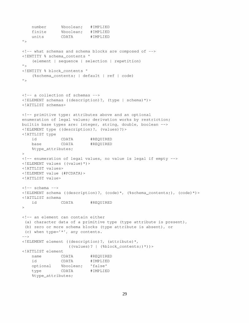
number %boolean; #IMPLIEDfinite %boolean; #IMPLIEDunits CDATA #IMPLIED

">

<!ENTITY % schema_contents "

(element | sequence | selection | repetition)"><!ENTITY % block_contents "

(%schema_contents; | default | ref | code)">

<!ELEMENT schemas ((description)?, (type | schema)*)><!ATTLIST schemas>

<!ELEMENT type ((description)?, (values)?)><!ATTLIST type

id CDATA #REQUIREDbase CDATA #REQUIRED%type_attributes;

><!ELEMENT values ((value)*)><!ATTLIST values><!ELEMENT value (#PCDATA)><!ATTLIST value>

<!ELEMENT schema ((description)?, (code)*, (%schema_contents;), (code)*)><!ATTLIST schema

id CDATA #REQUIRED>

<!ELEMENT element ((description)?, (attribute)*,

((values)? | (%block_contents;)*))><!ATTLIST element

name CDATA #REQUIREDid CDATA #IMPLIEDoptional %boolean; "false"type CDATA #IMPLIED%type_attributes;

29

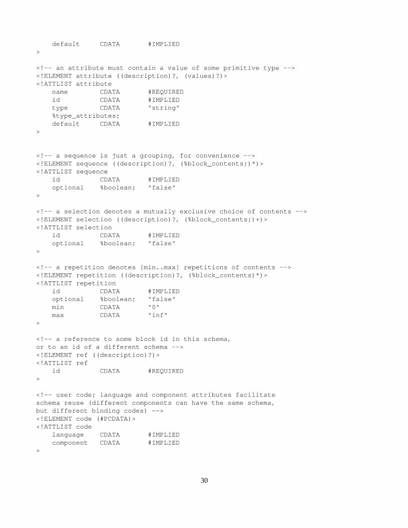
default CDATA #IMPLIED>

<!ELEMENT attribute ((description)?, (values)?)><!ATTLIST attribute

name CDATA #REQUIREDid CDATA #IMPLIEDtype CDATA "string"%type_attributes;default CDATA #IMPLIED

>

<!ELEMENT sequence ((description)?, (%block_contents;)*)><!ATTLIST sequence

id CDATA #IMPLIEDoptional %boolean; "false"

>

<!ELEMENT selection ((description)?, (%block_contents;)+)><!ATTLIST selection

id CDATA #IMPLIEDoptional %boolean; "false"

>

<!ELEMENT repetition ((description)?, (%block_contents)*)><!ATTLIST repetition

id CDATA #IMPLIEDoptional %boolean; "false"min CDATA "0"max CDATA "inf"

>

<!ELEMENT ref ((description)?)><!ATTLIST ref

id CDATA #REQUIRED>

<!ELEMENT code (#PCDATA)><!ATTLIST code

language CDATA #IMPLIEDcomponent CDATA #IMPLIED

>

30

<!ELEMENT default ANY>

<!ELEMENT description ANY>

31