btu-berkeley topography utilities for linking … for linking topography and impurity diffusion...
TRANSCRIPT

BTU-BERKELEY TOPOGRAPHY UTILITIES FOR LINKING TOPOGRAPHY AND IMPURITY DIFFUSION SIMULATIONS
by
Robert H. Wang
Memorandum No. UCB/ERL M91/71 August 27,1991


BTU - BERKELEY TOPOGRAPHY UTILITIES
FOR LINKING TOPOGRAPHY AND IMPURITY
DIFFUSION SIMULATIONS
by
Robert H. Wang
Memorandum No. UCBERL M9 ln 1
27 August 1991
ELECTRONICS RESEARCH LABORATORY
College of Engineering University of California, Berkeley
94720


BTU - Berkeley Topography Utilities for Linking Topography and Impurity Diffusion Simulations
Robert H . Wang
Department of Electrical Engineering and Computer Sciences University of California, Berkeley
ABSTRACT
This report chronicles the development of BTU (Berkeley Topography Utilities) for linking topography and impurity diffusion simulations. Currently implemented on the data structures in the SIMPL-2 program, BTU solves the problem of combining topography and mesh points by providing functions to map topographies between strings generated by topography simulators such as SAMPLE and polygons which can be decomposed into triangular meshes used by impurity diffusion simulators such as SUPREM-IV. To facilitate the integration of topography and impurity diffusion simulators, BTU also includes functions which make a rectangular grid conform to topography, and convert the topography and impurity concentrations between rectangular grid and tri- angular meshes. The procedural interface is high level in the sense that the functionalities provided by BTU are independent of the underlying SIMPL-2 data structures and geometric algorithms. This allows TCAD developers to add and maintain easily links to other simulators, and gives them the option to reimplement BTU functions for robusmess or efficiency as geometric modellers and adaptive grid generators becomes widely available. SIMPL-2 interfaces to SAMPLE and SUPREM-IV are used to demonstrate the procedural interface. Results and run times from SIMPL-IPX simulations of epitaxy with buried layers for submicron twin-well CMOS and BiCMOS processes and a 16-Mb DRAM trench capacitor are presented to demonstrate the simulation capabilities made possible by linking SAMPLE and SUPREM-IV through BTU and meas- ure the performance of the current BTU implementation.
August 18, 1991

In the memory of my father, Mr. Jan4 Wang, who influenced his children in ways he never
knew, provrded them with opportunities he never had, and loved them in ways they could never
repay.

Acknowledgement
First, I would like to thank my research advisor, Professor Andrew R. Neureuther for his
support and encouragement throughout this project. Without his vision, insight, and optimistic
enthusiasm, this project would never have been realized I would also Like to thank Professor
W.G. Oldham for reviewing this report. Thanks also go to Professor R.W. Dunon at Stanford
and Professor M.E. Law at University of Florida for useful discussions on SUPREM-IV.
Collaborations with (in alphabetical order by last names) Goodwin Chin at Stanford and
Andrej Gabara on SUPREM-IV, Ed Scheckler on SAMPLE and SUIPL-IPX, and Alex Wong
on TCAD frameworks are gratefully acknowledged. More than just isolated efforts to finish
pieces of an master’s project, these experience have helped me grow as a researcher and a pro-
grammer.
Personally, these past two years have been some of the more turbulent. I thank God for
pulling me through the hard times and blessing me with a wonderful support system full of
loving relatives and supportive friends. This report is dedicated to my mother.
The financial support from the Semiconductor Research Corporation, the California State
MICRO Program, IBM, and Motorola is gratefully acknowledged.


Table of Contents
1 . Introduction ....................................................................................................................................
1.1. Motivation ..........................................................................................................................
1.2. Integration of SAMPLE and SUPREM-IV in SIMPL-IPX ......................................
1.3. Organization .......................................................................................................................
2 . Background, Data Structures, and Algorithms ...................................................................
2.1. Background ........................................................................................................................
2.2. Data Structures ..................................................................................................................
2.3. Algorithms ..........................................................................................................................
2.3.1. Write-Top ...........................................................................................................
2.3.2. Stitch ....................................................................................................................
2.3.3. Get-Layers .........................................................................................................
2.3.4. Stitch-Back .........................................................................................................
2.3.5. MC-Grid .............................................................................................................
2.3.6. Mesh .....................................................................................................................
2.3.7. Unmesh ................................................................................................................
3 . Applications and Performance ..................................................................................................
3.1. Applications .......................................................................................................................
3.1.1. Epitaxy with Buried Layers ..............................................................................
3.1.2. 16-Mb DRAM Trench Process ........................................................................
1
1
3
4
6
6
7
8
9
9
9
10
1 1
12
13
14
14
14
16

3.2. Run Time Performance .................................................................................................... 17
4 . Conclusions ..................................................................................................................................... 18
4.1.Summary ............................................................................................................................. 18
4.2. Recommendations for Future Work .............................................................................. 18

List of Figures
Figure 1.1 Topography and Impurity Diffusion Interaction
Figure 13 Impurity Diffusion Equation
Figure 1.3 SIMPL-IPX System Organization
Figure 1.4 Berkeley Topography Utilities
Figure 15a Topography Simulation Interface
Figure 15b Impurity Diffusion Simulation tnterface
Figure 2.0 SIMPL-2 Data Structure
Figure 2.1 Write - Top
Figure 2.2 Stitch
Figure 2.3 Get - Layers
Figure 2.4a Stitch - Back
Figure 2.4b Work Out Top
Figure 2.442 Find - Intersect
Figure 2.4d Two D Search or Insert2
Figure 2.4e Clip - Polygon
Figure 25a MC - Grid
Figure 2.5b Find - Grid - Intersect
Figure 2 .5~ Add - Grid
Figure 2 J d Remove - Dense - Grid
- -
- - - -
Figure 2.6 Mesh
Figure 3.la Epitaxy with Buried Layers
Figure 3.lb SIMPL-DIX: Buried N+ Layer Implant and Drive-In
Figure 3.lc SIMPL-DE: Buried P Layer Implant
Figure 3.ld SUPREM-IV Mesh: Buried P Layer Implant
Figure 3.le SIMPL-DE: N Epitaxy
Figure 3.lf SUPREM-IV Mesh: Autodoping
Figure 3.lg SIMPL-DE: Epitaxy with Buried Layers
Figure 3.2a 16-h4b DRAM Trench Process
Figure 3.2b SIMPL-DIX: Trench Lithography
Figure 3 . 2 ~ SWL-DIX: Trench Etch
Figure 3.2d SAMPLE Suings: Trench Etch
Figure 3.2e SIMPL-DE: Trench Implant
Figure 3.2f SUPREM-IV Mesh: Trench Implant & Diffusion
Figure 3.2g SIMPL-DIX: Trench Diffusion
Figure 3.2h SIMPL-DIX: Trench Capacitor
Figure 3.3a Run Time Performance: Epitaxy with Buried Layers
Figure 3.3b Run Time Performance: 16-Mb DRAM Trench Process

1
1. Introduction
1.1. Motivation
Device scaling into the submicron regime has resulted in complex device topographies
which strongly influence impurity profiles and device behavior. To characterize and optimize
modem integrated circuit (IC) devices, it is critical to be able to explore accurately and
efficiently topography tradeoffs in device design. One cost effective way to perfom this task
is through integrated process and device simulation. Unfortunately, incorporating topography
simulation nsults into impurity diffusion and device simulations has remained a major obstacle
in the development of integrated process and device simulation systems. A key issue which
has not been systematically addressed is maintaining the consistency of topography and mesh
points at material interfaces.
Topography and mesh points are said to be consistent if they require little modification
when they are combined. Ideally, if one uses only data representations which allow efficient
implementations of both surface advancement algorithms and adaptive grid generation, such as
the octree representation used in i2 [l], topography and mesh points would always be con-
sistent However, typical topography simulators such as SAMPLE [2,3] and impurity diffusion
simulators such as SUPREM-IV [4.5] often use geometrically dissimilar data representations
such as strings and meshes. Furthermore, the user may wish to retain different levels of physi-
cal details in topography and impurity diffusion simulations. Hence, maintaining the consisten-
cy of topography and mesh points is a problem which must be addressed in linking most to-
pography and impurity diffusion simulators.
The problem of maintaining topography and mesh point consistency is especially complex

2
for highly nonplanar suuctures in which high topography point density is required to represent
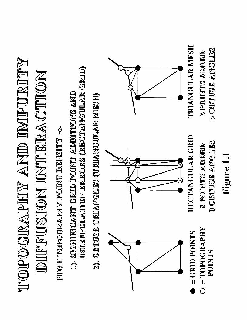
nonplanar surfaces. As Figure 1.1 illustrates, high topography point density adversely affects
the mesh represented using rectangular grids and mangular meshes common in impurity
diffusion simulators. In the case of a rectangular grid, combining topography points with the
grid requires many grid Line additions and results in significant interpolations of impurity con-
cenuation. For triangular meshes, there are two strategies for merging topography points into
the triangular mesh: merge with remesh and merge without remesh. Merging with remesh
results in significant interpolations of impurity concentrations, while merging without remesh
may create triangular elements with obtuse interior angles. Figure 1.2 shows why triangular
elements with obtuse interior angle are undesirable. As illustrated in Figure 1.2, the impurity
diffusion equation is solved numerically using The Divergence Theorem. An obtuse interior
angle causes error because it eniarges the area of integration used in the area integral and
changes the sign of the normal vectors used in the path integral.
This report chronicles the development of BTU (Berkeley Topography Utilities) for link-
ing topography and impurity diffusion simulations. Currently implemented on the data struc-
tures in the SIMPL-2 [6] program, BTU solves the problem of combining topography and
mesh points by providing functions to map topographies between strings generated by topogra-
phy simulators such as SAMPLE and polygons which can be decomposed into triangular
meshes used by impurity diffusion simulators such as SUPREM-IV. To facilitate the integra-
tion of topography and impurity diffusion simulators, BTU also includes functions which make
a rectangular grid conform to topography, and convert the topography and impurity concenua-
tions between rectangular grid and triangular meshes. The procedural interface is high level in
the sense that the functionalities provided by BTU are independent of the underlying SIMPL-2
data structures and geometric algorithms. This allows TCAD developers to add and maintain
easily links to other simulators. and gives them the option to reimplement BTU functions for

3
robusmess or efficiency as geometric modellers and adaptive
available. SIMPL-2 interfaces to SAMPLE and SUPREM-N
cedural interface. Results and run times from SIMPL-IPX
buried layers for submicron twin-well CMOS and BiCMOS
grid generators becomes widely
are used to demonstrate the pro-
[7] simulations of epitaxy with
processes and a 16-Mb DRAM
trench capacitor are presented to demonstrate the simulation capabilities made possible by link-
ing SAMPLE and SUPREM-IV through BTU and measure the performance of the current
BTU implementation.
12. Integration of SAMPLE and SUPREM-IV in SIMPL-IPX
An important goal of this project is to make SIMPL-IPX a viable tool for investigating
topography tradeoffs in device design by linking SAMPLE and SUPREM-IV. Another goal is
to make the geometric functions developed in this effort reusable for integrating other simula-
tors. To accomplish these goals, a high level procedural interface to access the geometric func-
tions was defined and SIMPL-IPX was reorganized to prove out this interface.
Figure 1.3 shows the current organization of SLMPL-IPX. Prominently displayed in this
figure are BTU (Berkeley Topography Utilities) and the simulator interfaces. Figure 1.4 illus-
trates major components of BTU. At the center of BTU is the geometric modeller which pro-
vides functions to traverse and query the data structures. Presently, functions which manipu-
late the SLMPL-2 polygon and grid data structure form the geometric modeller. One level
above the geometric modeller is the geometric toolkit which contains functions to perform
computations such as intersection finding and polygon clipping. BTU functions are implement-
ed using a combination of geometric modeller and toolkit functions. Presently, there are seven
BTU functions defined in the procedural interface. These functions include Write-Top, Stitch,
Get-Layers, Stitch-Back, MC-Grid, Mesh, and Unmesh. Write-Top converts the top sur-

4
face of the structure into a string. Stitch adds a polygon composed of a deposit string and the
top surface. Get-Layers converts the structure into a set of strings ordered from top to bot-
tom. Stitch-Back clips the structure against an etch string. MC-Grid adds grid lines to con-
form the rectangular grid to the topography. Mesh generates a triangular mesh using a topog-
raphy conforming rectangular grid. Unmesh maps impurity concentrations calculated a tri-
angular mesh onto a rectangular grid.
The BTU procedural interface facilitates the linking of additional topography and impuri-
ty diffusion simulatom by separating geomeuical data translation and modification from process
modeling. This concept is best illustrated by the SAMPLE and SUPREM-IV interfaces
currently in SLMPL-IPX. As shown in Figure lSa, interfaces to topography simulators such as
SAMPLE can be constn~cted using the Write-Top or Get-Layers utilities to create the input
strings, and the Stitch and StitchBack utilities to update the structure with the output suings.
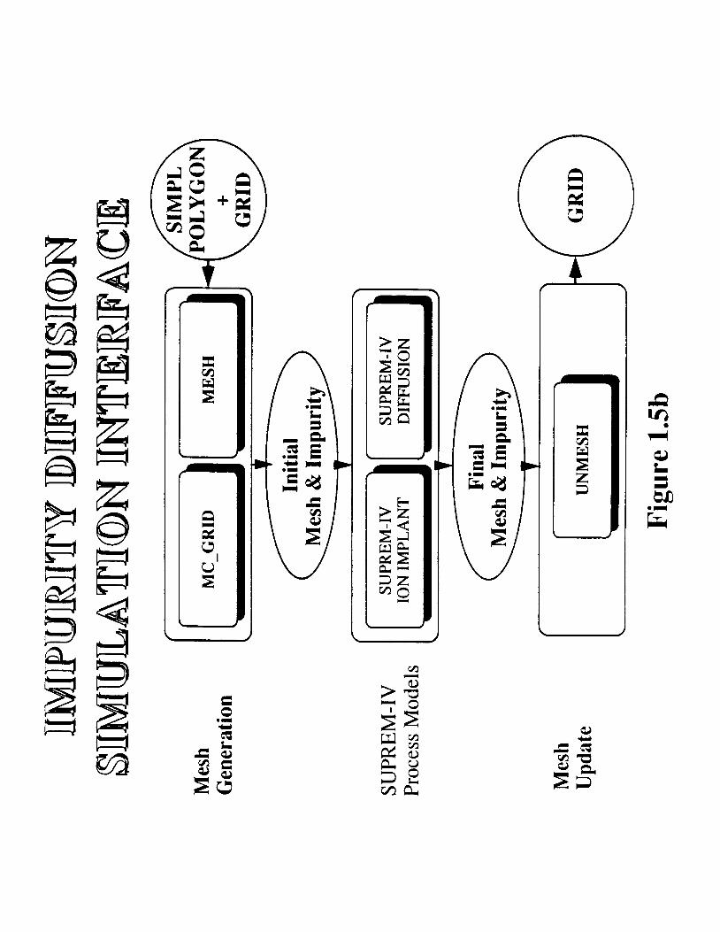
Similarly, Figure 1.5b shows that interfaces to impurity diffusion simulators such as
SUPREM-IV can use the MC-Grid and/or Mesh utilities to create the input mesh, and the
Unmesh utility to map the impurity xnuations back onto the topography conforming rec-
tangular grid. In both cases, the ? developer only need to generate model information
specific to hisher simulator and supply data converters between the simulator data format and
either SAMPLE strings or SUPREM-IV triangles.
1.3. Organization
The remainder of the report focuses on the implementation and applications of BTU.
Chapter 2 gives a historical account of the development of BTU and contains a detailed discus-
sion of the current implementation. Chapter 3 presents results and run times from SLMPL-IPX
simulations of epitaxy with buried layers for submicron twin-well CMOS and BiCMOS

5
processes and a 16-h4b DRAM trench capacitor. Chapter 4 concludes the report with a sum-
mary of the contributions of this project and recommendations for future work.
A 00
z @a a
I 0 0

U
rl
n > 'u e a
+ u

W
0 m

W
s 3.1
I B , l ‘ I ’ n n a w
E r \
c4
0 4 w 0 E n
W
w


6
2. Background, Data Structures, and Algorithms
2.1. Background
The origin of BTU can be traced back to the seminal work by Lee on the S W L - 2 pro-
gram. Lee introduced a polygon data svuc~re for topography simulation and a rectangular
grid data structure for impurity diffusion and device simulations. The geometric functions
which he implemented to traverse and query these data structures lay the foundation for the
geometric modeller currently used by BTU. Lee also implemented the first BTU algorithms,
the Write-Top and Stitch utilities, as part of the interface for SAMPLE deposition.
The next milestone in the development of BTU algorithms was the implementation of the
Get-Layers utility by Scheckler for etching and parasitic extraction of VLSI interconnects [SI.
To avoid the problem of clipping the svucture against the etch suing, Scheckler simulated
etching only on stlllctures covered by blanket deposition and updated these structures by delet-
ing the top polygon and adding the etch string to the structure using the Stitch utility. This
"strip and stitch" approach was also used later by Wang and Scheckler to update the structure
after lithography simulations [7].
The "strip and stitch" approach was, however, not adequate for simulating etching of
highly nonplanar structures such as the silicon trench. Furthermore, it was also recognized that
complete characterization of advanced IC device structures such as the silicon trench required
linking topography and impurity diffusion simulations. Thus, work began in Fall 1989 to ex-
tend the SAMPLE interface for general topography simulation and construct a SUPREM-IV in-
terface for ion implant and impurity diffusion simulations. By Spring 1990, collaborative
efforts between Wang at the University of California at Berkeley working on SIMPL-2 and

7
Chin at Stanford University working on SUPREM-IV resulted in SWL-IPX and successfully
demonstrated integrated topography and impurity diffusion simulations for a bipolar process
with self-aligned plysilicon emitter and polysllicon collector plug [7]. However, most of the
utility algorithms were embedded in the SAWLE interface in SIMPL-2 and SUPREM-IV pm-
cess modules and required rather circular operations to invoke. Consequently, the prototype
SIMPL-IPX lacked a clear structure to support modular growth of additional utility algorithms
or interfaces to other topography and impurity diffusion simulators.
The current definition and implementation of BTU came as the result of reorganizing
SIMPL-IPX to support modular growth. All BTU algorithms were either reimplemented or
developed during the reorganization. The Write-Top, Stitch, and Get-Layers utilities were
taken out of the SAMPLE interface and reimplemented as independent BTU functions. The
Stitch-Back utdity whch formerly relied on a pseudo plasma etching module in SUPREM-IV
was redesigned to work with utilities which operate directly on the SIMPL-2 rectangular data
structure. A MC-Grid utility was created u, make rectangular grids conform to topography.
Mesh and Unmesh utilities were created to transfer impurity concentrations between rectangu-
lar grids and triangular meshes.
2.2. Data Structures
The current implementation of BTU algorithms uses the SIMPL-2 polygon and grid data
structures which are illustrated in Figure 2.0. The polygon data structure is composed of a
linked list of polygons, each containing a loop of vertices and a material name, and a network
of vertices. Each vertex in the network contains the coordinates of the vertex, pointers to ver-
tices that follow it in the network, and the material names attached to the edges corresponding
to the venex pointers. The material names attached to an edge is that of the polygon on the

8
right side of the edge. Common polygon data smcture operation include Get-Left-Top,
Get-Right-Top, and Move. Get-Left-Top finds the vertex which 1) is exposed to air, 2) is
on the simulation window boundary, and 3) has an "x" value equal to "min".
Get-Right-Top performs a similar task except it finds the vertex that has an "x" value q u a i
to "xmax". Move takes as input a vertex and a material name, and returns the vertex at the
end of the edge that corresponds to the material name.
The grid data structure is made up of two one-dimensional arrays which store the loca-
tions of the vemcal and horizontal grid lines, and a three dimensional array which stores the
impurity concentrations. The first index of the three dimensional array indicates the type of
impurity, while the second and third indices of the three dimensional array point to the coordi-
nates of the grid point. In the current version of SIMPL-2, only boron and arsenic concentra-
tions are supported. Operations to insert and delete grid lines and rows and columns of impur-
ity concentrations are available. However, these operations are computationally expensive, i.e.
O(n2> where n is number of grid lines, because both the grid line and impurity concentrations
arrays are static.
2.3. Algorithms
There are currently seven functions defined in Lhe BTU procedural interface: Write-Top,
Stitch, Get-Layers, Stitch-Back, MC-Grid, Mesh, and Unmesh. The sections below
describe the functionalities of the utilities and the algorithms used in the current implementa-
tion.

9
23.1. Write-Top
The Write-Top utility converts the top surface of the smcture to a string. First,
Write-Top calls the Get-Left-Top and Get-Right-Top utilities to get the left and right end
points of the top string. Then, starting at the left end point, all the vertices which are exposed
to air are trave& until the right end point is reached. Figure 2.1 lists the pseudocode and il-
lustrates the Write-Top utility algorithm. A more detailed description is given in [61.
23.2. Stitch
The Stitch utility calls the Write-Top utility to get the top surface of the structure and
then adds a polygon composed of a deposit sving and the top surface. The new polygon is
created by connecting the end points of the deposit string and the top surface. The pseudocode
and a pictorial description of the Stitch utility is given in Figure 2.2. A more detailed descrip-
tion can also be found in [6 ] .
23.3. Get-Layers
The Get-Layers utility convem the structure into a set of strings ordered from top to
bottom by successively deleting polygons and calling the Write-Top utility. The most impor-
tant component of the Get-Layers utility algorithm is the Find-Top-Polygon function, which
determines if a polygon sits on top of all the other polygons in the structure. A detailed
description of the criteria used to determine the "top polygon" is in [8]. Figure 2.3 outlines
and illustrates the effects of the Get-Layers algorithm.

10
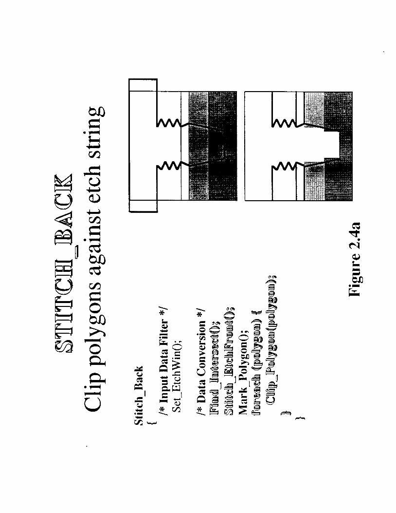
23.4. Stitch-Back
The Stitch-Back urility clips the smcture against an etch string by finding and inserting
into the suucture intersections between the polygons and the etch string, stitching together the
intersections and string points into a linked list of vertices, and clipping the polygons in the
structure using the etch string represented by the linked list of intersection and saings. figure
2.4a gives the pseudocode which outlines the major steps in the Stitch-Back operation.
To ensure that CPU time is not wasted sifting through collinear or relatively collinear
points during the Stitch-Back operation, a geometric toolkit function, Work-Out-Top, is
usually invoked before Stitch-Back to filter the etch suing. As shown in Figure 2.4b,
Work-Out-Top throws out string points which join segments that are extremely short or have
equal slopes.
The task of finding and inserting intersections is performed by the geometric toolkit func-
tion Find-Intersect illustrated in Figure 2 .4~ . As shown in Figure 2.4c, Find-Intersect is a
brute force, Own) algorithm which compares N polygon segments against n string segments.
Intersections computed by Find-Intersect are inserted into the structure and sorted by their re-
lative distances to string points for use in the stitching stage. In the current implementation of
Stitch-Back, most of the CPU time is spent on Find-Intersect since it is an Own) operation.
By comparison, stitching the intersections and string points is an O(n) operation and the
Clip-Polygon algorithm is Ow). However, by calling Work-Out-Top before Stitch-Back
with a tolerance of 1.Oe-06, most etch strings can be rcduccd down to below 400 points, and
can be processed by Stitch-Back in about 10 CPU seconds on an IBM RS/6000 Model 530.
The computation of intersections is actually done using the geometric modeller function
Two-D-Search-or-Insert2. Using a test which checks if a point lies counter-clockwise, col-

11
linear, or clockwise to a segment, Two-D-Search-or-Lnsert2 determines if an intersection
exists between a polygon segment and a string segment by testing if 1) the polygon vertices lie
on opposite sides of the string segment and 2) the string points lie on opposite sides of the po-
lygon segment [9]. Cases covered by this criterion are illustrated in Figure 2.4d. If an inter-
section does exist, Two-D-Search-or-Insert2 calculates the coordinates of the intersection by
paramemzing the polygon and string line segments using the standard y = mx + b form and
solving the resultant system of line segment equations. The intersection is inserted into the
suuchlre using the geometric modeller function Insert, which properly establishes connectivity
between the intersection and vertices originally in the smcture.
The geometric toolkit function Clip-Polygon is used to cut polygons with an etch string
represented as a linked list of intersections and string points. For each polygon, Clip-Polygon
first determines if the polygon should be deleted, clipped, or kept in tact. For polygons whch
are clipped, Clip-Polygon first identifies all the cuts into the polygon made by the etch string
and then traverse these cuts and some of the original polygon vertices to create one or more
polygons. Figure 2.4e illustrates how Clip-Polygon uses cuts to create new polygons. Experi-
ence with Stitch-Back has shown the robusmess of Stitch-Back depend heavily on the
robusmess of Clip-Polygon. The current version of Clip-Polygon works well for cutting
structures such as lines and trenches and updating etchback away from material interfaces, but
is less successful at updating etchback close to material interfaces.
2.3.5. MC-Grid
MC-Grid, which is short for Make-Conform-Grid, defines the topography on the rec-
tangular grid by finding and inserting into the structure intersections between the polygons and
the grid lines, adding grid lines at all polygon vertices, and removing grid lines which are sur-
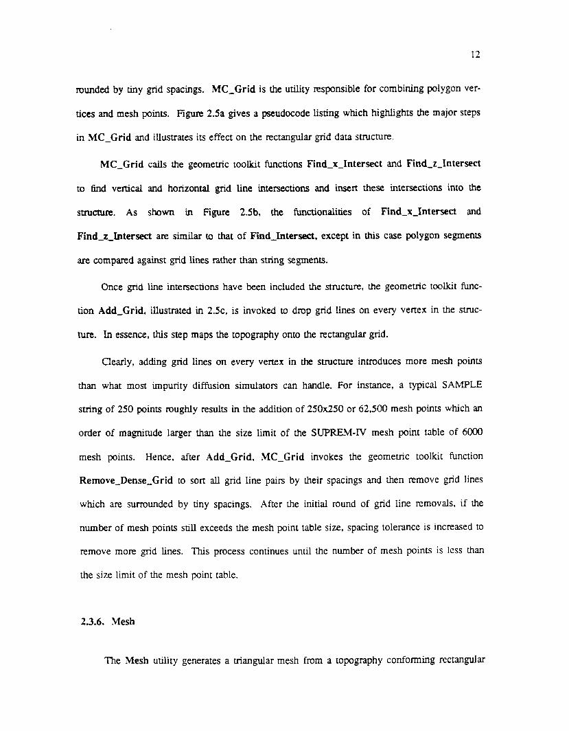
rounded by tiny grid spacings. MC-Grid is the utility responsible for combining polygon ver-
tices and mesh points. Figure 2.5a gives a pseudocode listing which highlights the major steps
in MC-Grid and illustrates its effect on the rectangular grid data structure.
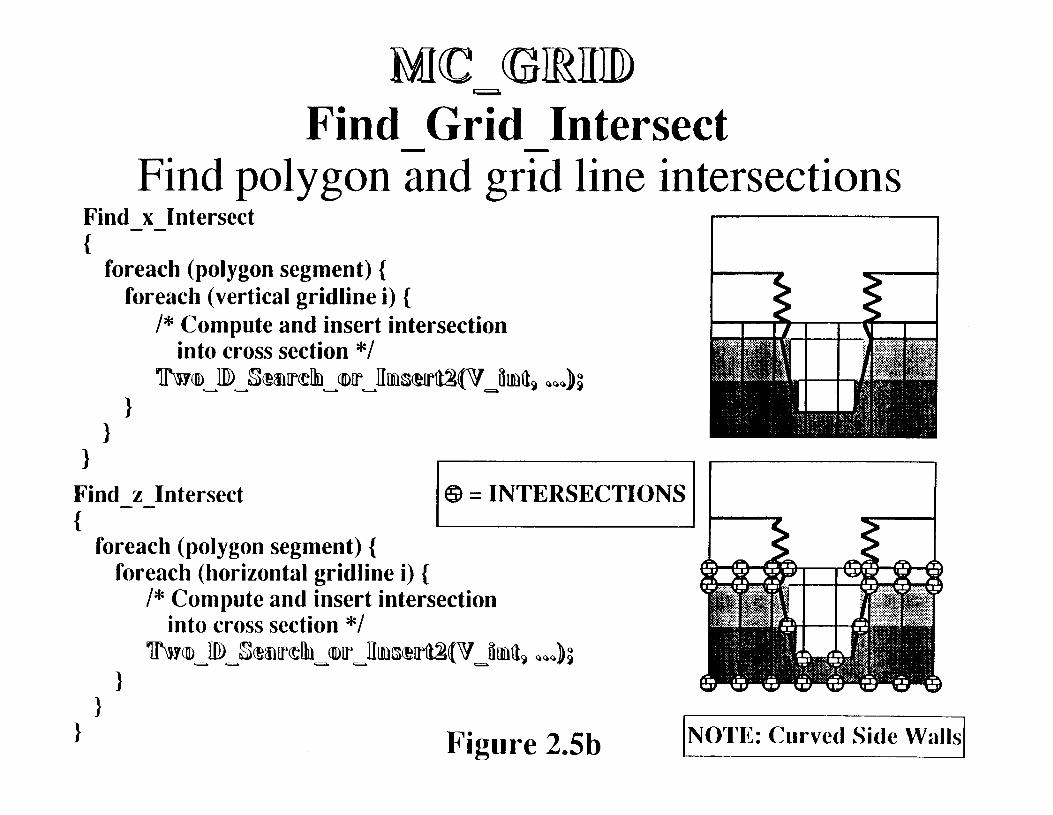
MC-Grid calls the geometric toolkit functions Find-x-Intersect and Find-z-Intersect
to find vertical and horizontal grid line intersections and insen these intersections into the
structure. As shown in Figure 2Sb, the functionalities of Find-x-Intersect and
Findz-Intersect are similar to that of Find-Intersect, except in this case polygon segments
are compared against grid lines rather than string segments.
Once gnd line intersections have been included the structure, the geometric toolkit func-
tion Add-Grid, illustrated in 2Sc, is invoked to drop grid lines on every venex in the struc-
ture. In essence, this step maps the topography onto the rectangular grid.
Clearly, adding grid lines on every vertex in the structure introduces more mesh points
than what most impurity diffusion simulators can handle. For instance, a typical SAMPLE
string of 250 points roughly results in the addition of 250x250 or 62,500 mesh points which an
order of magnitude larger than the size limit of the SUPREM-IV mesh point table of 6000
mesh points. Hence, after Add-Grid, MC-Grid invokes the geometric toolkit hnction
Remove-Dense-Grid to son a l l grid line pairs by their spacings and then remove grid lines
which are surrounded by tiny spacings. After the initial round of grid line removals, if the
number of mesh points still exceeds the mesh point table size, spacing tolerance is increased u)
remove more grid lines. This process continues until the number of mesh points is less than
the size limit of the mesh point table.
2.3.6. Mesh
The Mesh utility generates a triangular mesh from a topography conforming rectangular

13
grid. The assumption that the topography is defined at grid points greatly simplifies the algo-
rithm since it implies that string segments would lie on the diagonals of the rectangular ele-
ment. Figure 2.6 outlines the .Mesh algorithm and illustrates its output
23.7. Unmesh
The Unmesh utility maps the impurity concentrations from a triangular mesh back to the
rectangular grid. The major limitation of Unmesh is that it assumes the topography does not
change during impurity diffusion. Consequently, this means oxidation during impurity
diffusion is not currently supported by BTU.

L L
Iz 0 c,
J 0
n l+
I
N I
c 0
n 1 I
x I
E
L L = U
X 0 0

d v , *
E 0
Q) > r=
o n
13
.e X Q)
L Q) > c,
+ n X Q)
L Q) > c,
o m X Q)
L Q) > c,
II
.e L a .I
2 o n
c, ep E 0 u a G
X Q)
t aJ > X Q) E II X Q)
L Q) *
c,
c, - c,
c)
c j aJ L 3

cs, 0 I

Convert polygons to strings Get - Layers {
Save cross section;
/* Data Conversion */ n layers = 0; wiiile (more polygons left) {
layers[n layers] =Write n layers++; Finnd "topt1 polygon; Delete "top" polygon;
1
Restore cross section;
/* Output Data Filter */ Remove redundant layers;
1
Figure 2.3
1 * E 0 cn L Q)
.I

Work Out TOD Filter collinear or dense string points
s1 S l
S l
$ s2 s2
s2
(S1,S) and (S,S2) has Same Slope Very Short ID@R@O@ s D@RSU(e $3
(S1,S) and (S,S2) are (S1,S) and (S,S2) Have Different Slope and are Long K9ep s
Figure 2.4b

Find Intersect Find polygon and string intersections
Find - Intersect {
foreach (polygon segment) { foreach (string segment i) {
/* Compute and insert intersection into cross section */
muD u u ID Search - - or IIrnsserap - firmu, o'ao);
/* Insert intersections into a
Insert - Etch(IntList[i], V - int, ...); sorted link list of intersections */
@ = INTERSECTIONS
Figure 2 . 4 ~

Two D Search or Insert2 Find polygon and string segment intersections
v1
S l g2 v 2
Different Slope and IIrmterprs~3
v 2
S l 0 AS2 e
Different Slope and NmO l[~.~Oerpr~mQ
0 =VERTICES
0 = STRING POINTS
Q = INTERSECTIONS
Figure 2.4d
P s2
S l 0 %e v2
Intersect is anvertex
V l
s1 0 71 v2
Infinite Slope

E 0 ba h
I & h.
o =
CI n
I
aa & 3 w k .m

MC L GRID Make rectangular grid conform
to the topography MC - Grid c
/* Input Data Filter */ Save cross section; Delete - Row();
/* Data Conversion */ Add - Grid[);
1 NOTE: curved ~ i c ~ e ~ a ~ ~ s 1
MC - GRED Find - Grid - Intersect
Find polygon and grid line intersections Find - - x Intersect {
foreach (polygon segment) { foreach (vertical gridline i) {
/* Compute and insert intersection into cross section *I
muD v u ID s@$Ircb - 0 @Do" I I m S Q r p a ~ c. irnt&w&
I Find - - z Intersect
foreach (polygon segment) {
G = INTERSECTIONS
foreach (horizontal gridline i) {
into cross section */ /* Compute and insert intersection
Two u u D Semreb u u UDr 1
Figure 2.5b

Add Grid
Add Horizontal Grid Line at z;
Drop grid lines on vertices
= VERTICES
IBIaDriz@rrmhn Grid Lfine IImQ@rsmufiaDm QXQB) : Add Vertical Grid Line at x; Interpolate doping along x;
veruian mid I M D ~ ~~muer~~atfiQm CIX,~) : Add Horizontal Grid Line at z; Interpolate doping along z;
Interpolate doping along z; @ = INTERSECTIONS
Figure 2 . 5 ~ (Assume Curved Side Wall 1

L cp a, .I
* *

Generate triangular mesh from rectangular
Mesh
/* Input Data Filter:
Read cross section; foreach (xz pair)
Generate valid grid points */
if ((x,z) is in cross section) Write grid point;
/* Data Conversion: Generate triangles */
foreach (rectangular element) if (element is in bulk)
Write both triangles; else if (element is at surface)
Write conforming triangle; 1
grid
I
Figure 2.u

14
3. Applications and Run Time Performance
3.1. Applications
3.1.1. Epitaxy with Buried Layers
Simulation of epitaxy with a buried layer implant is a simple yet practical example for
vetlfying the links to SAMPLE and SUPREM-IV. Figure 3.la lists the key steps in an epitaxy
process sequence with buried layer implants. Similar process sequences are used used in sub-
micron twin-well CMOS and BiCMOS processes [lo]. Processing begins with a 580 A oxide
growth whch is followed by an 800 A pad nitride deposition. A window is opened at the
center of the mask for an arsenic buried N+ layer implant of 1.Oe+15 cm-* and 80 keV. A
diffusion step of 25 minutes and 1100 C is used to drive-in the buried N+ layer implant. The
oxide growth during the diffusion step is simulated analpcally using SIMPL-2. Using the
field oxide as a mask, a boron buried P layer implant of 1.Oe+15 cm-* and 80 keV is intro- -
duced. After an N epitaxial growth of 1.3 um and 1.Oe+15 ~ m - ~ , a diffusion step of 5 minutes
and 1100 C is used to activate the buried P layer implant and simulate autodoping.
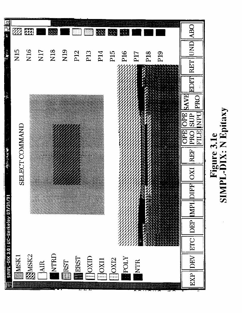
Figure 3.lb shows the cross section after the activation of buried N+ layer. Results from
the buried P layer implant are shown in Figure 3.lc while Figure 3.ld plots the corresponding
SUPREM-IV mesh. The cross sections before and after the autodoping simulation are shown
Figures 3.le and 3.lg respectively. Figure 3.lf shows the SUPREM-IV mesh tuned to simulate
autodoping. For epitaxy and film deposition, several horizontal grid lines must be added to the
grid generated by MC-Grid to capture doping transitions in the deposited material. Meshes
generated by only BTU functions would be devoid of mesh p in ts in the bulk of the deposited

15
material because Stitch does not place any polygon vertices along the edges of the deposited
polygon and LMC-Grid places grid lines only on polygon vertices.


NT19 SELECT C O M W D
1Y ILI
N13
N 14
N15
N 16
N 17 N 18
N 19
P12
P13
Figure 3.1b SIMPIJ-DIX: Suried N+ Layer Implant and Drive

II k
E

y in microns
i 0.00
-1o.ox10 -2
-0.20
-0.30
-0.40
-0.50
-0.60
-0.70
-0.80
-0.90
- 1 .oo -1.10
- 1.20
-1.30
- 1.40
- 1 S O
- 1.60
-1.70
- 1.80
- 1.90
-2.00
SUPREM-IV A.9130
i i erid
x in microns 0.00 0.50 1 .oo 1 S O
Figure 3.ld SUPREM-IV Mesh: Buried P Layer Implant
m s

0 C c L 0
&
C
rl
r(
x
Figure 3.1f SUPREM-IV Mesh: Autodoping


16
3.1.2. 16-Mb DRAM Trench Process
Trench process simulation is an excellent performance benchmark for BTU functions due
to the topographical complexity and the strong topography and impurity profile interaction in-
herent in trench structures. Figure 3.2a outlines the major steps of a 16-Mb DRAM trench pro-
cess similar to the one described in [ 111. First, several layers of materials are vertically depo-
sited using SIMPL-2. These layers include an P epitaxial layer of 2 um and 1.Oe+13 and
a 5000 A oxide-nitride-oxide (0-N-0) sandwich. After resist spin-on, g-line lithography and
plasma etching are sequentially invoked to dig a trench approximately 1 um wide and 5 um
deep. An arsenic implant of 1.Oe+12 cm-* and 200 keV is performed on the trench followed
by a diffusion step of 7 minutes and lo00 C. Trench oxidation during the diffusion step is
simulated by a 150 A conformal oxide deposition. The trench capacitor is formed by filling
the trench with with 0.7 um of N+ polysilicon doped at 1.Oe+20 ~ m - ~ .
Figures 3.2bc show the SIMPL cross sections after trench lithography and etching. The
SAMPLE etch strings used as input to the Stitch-Back utility are plotted in Figure 3.2d. Fig-
ures 3.2e and 3.2g plot the SIMPL cross sections before and after activation of the arsenic
trench implant. The SUPREM-IV mesh used to simulate the implant and diffusion is shown in
Figure 3.2f. The complete trench capacitor is shown in Figure 3.2h.

W El h
E l es, z El P3 b”
z 37
h
U
& z
n
n
W & 0
a a 0 0 0 0 a

a ...... ...... . . . . . .
. . . . . . . . . . .
. . . . . . . . . . . . . . . .
. . . . ...... - _.....-._... -..-..- .............. .......... .........-. ...................... .... ..............-. ...... .- ... ._ ... .-. ....... _- -. ...... .-. .--...... ...... - ... ."- .... ... ... .- ... ... ...-. ......-I-....-.
... ---- .- ...... -. ...... -- ......... .... .... --._ ........ -.
.... ...-.............
....... ............-. ....... ............-.
... -..-- ......... .-. ...................... ............ I ..... -. ......................
......................
...................... ................ "-. ... ." ......... ...-. .................. -. ...................... ......................
...................... _.. _.. _.. _.. _.. _.._.._
r A
G ......... Q ......... ......... Y 4 I!
n I 1 w
& E r VI

. .___. . . . . ..-. ..-. . ..-. . .- . .... _ _ .;: . . .-. .-. 1;:: . - . . . . . . . . . . --. . . .- ~
. . . . .-. I :::I;;;, . .
.. .-. . . . . . . . . . . ._. . . . . . . - . . .__
. . . . . . . . . . . . . . . . . . . . . . .
. . . . . . . . . . . . .
. .
. . . . . . . . . . . . . . .

i i
X-Y LINE PLOT
I \ I 1 1 1 IL ' I l l
X-AXIS i I ' I
i I 1
4 4
I
1.68
Figure 3.2d SAMPLE Strings: Trench Etch

c
.... :-- : . . r-- :. .....
. . . . . . . .
.. . . . . ,q:/: . . .
. ._I . . . . . . . . . . . . . . . . . . . -
c, E e8 0 E
- CI
m c

OpCOT/Xll t ~ o l 1 .l
e C c c C
z C
-1
i
h
Figure 3.2f SUPREM-IV Mesh: Trench Implant & Diffusion

. . .. . . . ___ . . , . . J ! : .-- I::.. ... .
. . . . . - .. . . . . . . . . . . . . .
. . . . ,
... , . , , . , . . . .
E M m

a
E
17
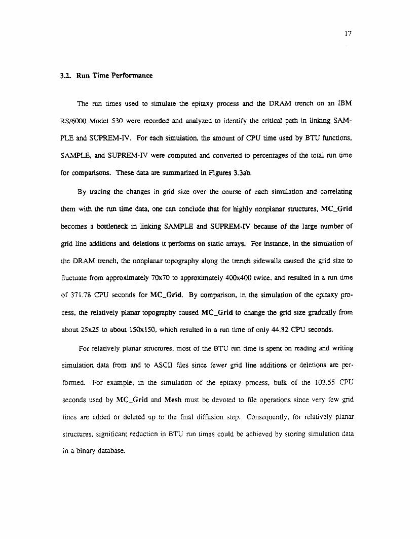
3.2. Run Time Performance
The run times used to simulate the epitaxy process and the DRAM trench on an IBM
RS/6000 Model 530 were recorded and analyzed to identify the critical path in linking S A M -
PLE and SUPREM-IV. For each simulation, the amount of CPU time used by BTU functions,
SAMPLE, and SUPREM-IV were computed and converted to percentages of the total run time
for comparisons. These data are summarized in Figures 3.3ab.
By tracing the changes in grid size over the course of each simulation and correlating
them with the run time data, one can conclude that for highly nonplanar structures, MC-Grid
becomes a bottleneck in linking SAMPLE and SUPREM-IV because of the large number of
grid line additions and deletions it performs on static arrays. For instance, in the simulation of
the DRAM trench, the nonplanar topography along the trench sidewalls caused the grid size to
fluctuate from approximately 70x70 to approximately 400x400 twice, and resulted in a run time
of 371.78 CPU seconds for MC-Grid. By comparison, in the simulation of the epitaxy pm-
cess, the relatively planar topography caused MC-Grid to change the grid size gradually from
about 25x25 to about 150x150, which resulted in a run time of only 44.82 CPU seconds.
For relatively planar structures, most of the BTU run time is spent on reading and writing
simulation data from and to ASCII files since fewer grid line additions or deletions are per-
formed. For example, in the simulation of the epitaxy process, bulk of the 103.55 CPU
seconds used by MC-Grid and Mesh must be devoted to Ne operations since very few grid
lines are added or deleted up to the final diffusion step. Consequently, for relatively planar
structures, sigmficant reduction in BTU run times could be acheved by storing simulation data
in a binary database.

EPITAXY with BURIED LAYERS
Figure 3.3a

Stitch - Back = 12.40 sec
0MC - Grid = 371.78 sec Mesh = 134.25 sec
Lithography = 4.48 sec
Implant = 22.60 sec
Diffusion = 553.27 sec Figure 3.3b

18
4. Condusions
4.1. Summary
The primary focus of this project has been the development of a set of functions, BTU, to
address the topography and mesh point consistency problem which arises in the linking of to-
pography and impurity diffusion simulations. In addition, a high level procedural interface for
accessing BTU functions has k e n defined to facilitate the extension and maintenance of simu-
lator interfaces and give TCAD developers the option to improve the robustness and efficiency
of BTU functions by incorporating geometric modellers and adaptive grid generators. Simula-
tions of epitaxy with buried layers for twin-well CMOS and BiCMOS processes and a 16-Mb
DRAM trench capacitor were used to verify the links to SAMPLE and SUPREM-IV. For
most structures, BTU string utilities such as Stitch-Back require on the order of 10 CPU
seconds on an IBM RS/6000 Model 530. The run time of BTU grid and mesh utilities such as
MC-Grid varies greatly with grid size, which depends directly on topographical complexity.
In particular, the MC-Grid utility has been identified as a bottleneck in linking SAMPLE and
SUPEM-IV for highly nonplanar structures such as the trench,
4.2. Recommendations for Future Work
First of all, the run time of the MC-Grid utility needs to be reduced. This can be ac-
complished by modifying the MC-Grid algorithm and changing the rectangular grid data
structure. The MC-Grid algorithm should be modified to avoid adding grid lines which are
likely to be removed in the latter stages of the MC-Grid operation. The rectangular grid data

19
structure which MC-Grid is implemented on should be dynamic to reduce the computational
cost of grid line additions and removal.
Secondly, the Unmesh uulity should be extended to handle oxidation during impurity
diffusion The extension involves modifjmg Unmesh to incorporate oxidation induced topogra-
phy changes into the polygon and rectangdar grid data structures. This will enable using BTU
to facilitate rigorous simulations of process sequences such as LOCOS and trench oxidation
Finally, the Clip-Polygon function used in the Stitch-Back algorithm should be im-
proved to handle more robustly etch strings which are close to material interfaces. This will
improve the overall robustness of Stitch-Back for updating etchback.
References
Conti, P.. Hitschfeld, N., and Fichmer, W., "Q - An Ocuee-Based LMixed Element Grid Allocator for Adaptive 3D Device Simulation", NUPAD III Technical Digest, pp. 25-26, June 1990. Oldham, W.G., Nandgaonkar, S.N., Neureuther, A.R., and O'Toole, M., "A General Simulator for VLSI Lithography and Etching Processes: Part I - Application to Projection Lithography", IEEE Trans. Electron Devices, vol. ED-26, pp. 717-722, August 1979. Oldham, W.G., Neureuther, A.R., Sung, C., Reynolds, J.L., and Nandgaonkar. S.N.. "A General Simulator for VLSI Lithography and Etching Processes: Part I1 - Application to Deposition and Etching", IEEE Trans. Ekctron Devices, vol. ED-27, pp. 1455-1459, August 1980. Law, M.E., Two Dimemiona1 Numerical Simulation of Impurity D i m i o n , PbD. thesis, Stanford University, January 1988. Rafferty, C.S.. Stress Eflects in Silicon Oxidation - Simulation and Experiments, Ph.D. thesis, Stanford University, December 1989. Lee, K., SIMPL-2 (SIMubed Profiles from Layout - Version 2), Ph.D. thesis, UC Berke- ley, July 1985. Scheckler, E.W., Wong, A.S., Wang, R.H., Chin, G.R., Camagna, J.R., Toh, K.K.H., Tadros, K.H., Ferguson, R.A.. Neureuther. A.R.. Dutton, R.W., "A Utility-Based Integrated Process Simulation System", 1990 Symposium on VLSI Technology: Digest of Technical Papers, pp. 97-98, June 1990. Scheckler, E.W., Extraction qf Topography Dependent Electrical Characteristics from Process Simulation using SIMPL, with Applications to Planarization and Dense Intercon- nect Technologies, MS report. UC Berkeley, December 1988. Sedgewick, R., Algorithms, 2nd Edition, Addison-Wesley Publishing Co., Reading, MA, 1988.
[lo] Haken, R.A., Havemann, R.H., EWund, R.H., and Hutter. L.N., "BiCMOS Process Tech- nology", BiCMOS Technology and Applications, Alvarez, A.R., Editor, Kluwer Academic Publishers, Boston, MA, 1989.
[111 Bakeman, P., Bergendahl, A.. Hakey, M., Horak, D., Luce, S., Pierson, B., "A High Per- formance 16-Mb DRAM Technology", 1990 Symposium on VLSI Technology: Digest of Technical Papers, pp. 11-12. June 1990.
