Bubble Treemaps for Uncertainty Visualization

Jochen Gortler, Christoph Schulz, Daniel Weiskopf, Member, IEEE Computer Society, and Oliver Deussen

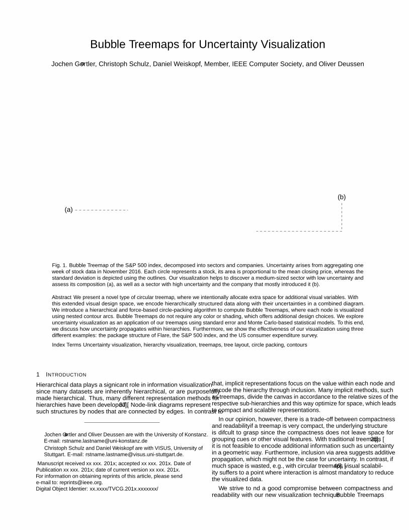
(a)

(b)

Fig. 1. Bubble Treemap of the S&P 500 index, decomposed into sectors and companies. Uncertainty arises from aggregating oneweek of stock data in November 2016. Each circle represents a stock, its area is proportional to the mean closing price, whereas thestandard deviation is depicted using the outlines. Our visualization helps to discover a medium-sized sector with low uncertainty andassess its composition (a), as well as a sector with high uncertainty and the company that mostly introduced it (b).

Abstract—We present a novel type of circular treemap, where we intentionally allocate extra space for additional visual variables. Withthis extended visual design space, we encode hierarchically structured data along with their uncertainties in a combined diagram.We introduce a hierarchical and force-based circle-packing algorithm to compute Bubble Treemaps, where each node is visualizedusing nested contour arcs. Bubble Treemaps do not require any color or shading, which offers additional design choices. We exploreuncertainty visualization as an application of our treemaps using standard error and Monte Carlo-based statistical models. To this end,we discuss how uncertainty propagates within hierarchies. Furthermore, we show the effectiveness of our visualization using threedifferent examples: the package structure of Flare, the S&P 500 index, and the US consumer expenditure survey.

Index Terms—Uncertainty visualization, hierarchy visualization, treemaps, tree layout, circle packing, contours

1 INTRODUCTION

Hierarchical data plays a significant role in information visualizationsince many datasets are inherently hierarchical, or are purposefullymade hierarchical. Thus, many different representation methods forhierarchies have been developed [37]. Node-link diagrams representsuch structures by nodes that are connected by edges. In contrast to

• Jochen Gortler and Oliver Deussen are with the University of Konstanz.E-mail: firstname.lastname@uni-konstanz.de

• Christoph Schulz and Daniel Weiskopf are with VISUS, University ofStuttgart. E-mail: firstname.lastname@visus.uni-stuttgart.de.

Manuscript received xx xxx. 201x; accepted xx xxx. 201x. Date ofPublication xx xxx. 201x; date of current version xx xxx. 201x.For information on obtaining reprints of this article, please sende-mail to: reprints@ieee.org.Digital Object Identifier: xx.xxxx/TVCG.201x.xxxxxxx/

that, implicit representations focus on the value within each node andencode the hierarchy through inclusion. Many implicit methods, suchas treemaps, divide the canvas in accordance to the relative sizes of therespective sub-hierarchies and this way optimize for space, which leadsto compact and scalable representations.

In our opinion, however, there is a trade-off between compactnessand readability—if a treemap is very compact, the underlying structureis difficult to grasp since the compactness does not leave space forgrouping cues or other visual features. With traditional treemaps [25],it is not feasible to encode additional information such as uncertaintyin a geometric way. Furthermore, inclusion via area suggests additivepropagation, which might not be the case for uncertainty. In contrast, ifmuch space is wasted, e.g., with circular treemaps [46], visual scalabil-ity suffers to a point where interaction is almost mandatory to reducethe visualized data.

We strive to find a good compromise between compactness andreadability with our new visualization technique: Bubble Treemaps.

They allocate extra space in the layout to encode certain and uncer-tain information together in a geometric manner, similar to error bars.Leaf nodes of a hierarchy are encoded as circles and enclosed by anarc-based parameterizable contour. Contours of sibling sub-hierarchiesare packed using a force-directed model and enclosed by another pa-rameterizable contour. This process is recursively continued until thewhole tree is traversed. This way, we can encode additional group-levelinformation, such as uncertainty, into the visual representation of thecontours. Figure 1 shows a typical example of a Bubble Treemap,emphasizing nodes with high uncertainty using deformations of thecontour (amplitude and frequency) to resemble variability of box-plotswhile maintaining treemap-typical color coding of higher-level nodes.

We consider uncertainty as a distribution of possible values per node,as opposed to a single and exact value. Showing the mean value aloneis often not sufficient to describe a distribution. Instead, we need visual-izations that are capable of displaying additional statistical features thathelp the reader gain a better understanding of the data. Many visualvariables do not work well for illustrating uncertainty [29]. As notedby Hullmann [24], uncertainty visualization is error-prone, especially,when drawing false conclusions because of bad communication regard-ing the underlying statistical model, e.g., confusing standard deviationwith variance. Our technique offers great flexibility to choose appropri-ate encodings, depending on the task and underlying model—it evenworks well in black and white.

Our contribution is threefold: First, we propose a layout based oncircle packing to use space purposely, achieving a reasonable trade-offbetween a compact representation of the hierarchy and its inherentinformation. Second, we define node contours analytically, resulting ina new parameter domain to be used for additional visual variables, inparticular, for uncertainty visualization. Third, we describe differentmodels of uncertainty and discuss their relation to hierarchal data. Ourdiscussion is rounded up by demonstration of our technique using threeexample data sets. An implementation of Bubble Treemaps can befound online1.

2 RELATED WORK

The following section gives an overview of work related to our method.First, we review the state of the art in visualizing hierarchical data.Next, we provide a summary of recent work for visualizing set mem-berships, since this topic is closely related to how our method encodesthe topology of an underlying tree structure. At last, we describe recentmethods of uncertainty visualization for graphs.

Visualization of Hierarchical Data There are many differentmethods to visualize hierarchical data; Schulz et al. [38] provide anextensive survey of implicit hierarchy visualization. Treemaps havebeen shown to be effective at conveying hierarchical information. Mostof the traditional treemap approaches, such as Squarified Treemaps [11]or Voronoi Treemaps [4] follow a top-down strategy, recursively subdi-viding a given area according to the underlying hierarchy. Similarly,Auber et al. [3] describe a treemap layout algorithm that produces ir-regular nested shapes by subdividing the Gosper curve. The boundariesof the areas, however, are not incorporated explicitly into the layout—the contours are inlaid retroactively and not used to encode additionalquantitative values.

Circle packing has been widely studied in theoretical computerscience, especially for its connection to planar graphs [14]. Stephen-son [40] provides a summary of the general field of circle packing.Usually, a more pragmatic approach is pursued for its application tohierarchy visualization: Wetzel [44] and Wang et al. [43] propose meth-ods based on nesting circles in a bottom-up fashion, which is laterrefined by Zhao and Lu [46]. Viegas et al. [42] use a combination ofcircle packing together with a balloon layout to visualize informationflow in social networks. Several domain-specific works combine densepacking of circles with layout methods from graph drawing such asBubble Trees or radial layouts [2, 23]. We utilize the method by Wanget al. to create our initial packings (Figure 2).

1https://github.com/grtlr/bubble-treemaps

McGuffin and Robert [30] provide an extensive study on the spaceefficiency of different tree representation methods. They introduce anovel metric that aims to measure the distribution of area across nodesin hierarchical visualizations. One conclusion of their work is that aperfect partitioning of the space might not be ideal when additionalinformation (for example labels) needs to be displayed. Similarly,Schulz et al. [38] argue that packing the space too tightly conceals theunderlying structure and methods that deliberately leave empty spacewould enable a better perception of the tree structure. These findingswere an inspiration for us when developing Bubble Treemaps.

Bubble charts are often used to visualize three-dimensional data. Tocreate a bubble chart, two dimensions are mapped to the x and y axesof the plane, while the third dimension is mapped to the size of a circleat the corresponding position. Bubble charts are commonly used onwebsites [12, 18], often they are part of an interactive exploration toolfor the data. Sometimes, however, either the category of the entities ortheir hierarchical structure is lost.

(a) Circular Treemap (b) Bubble Treemap

Fig. 2. Bubble Treemaps are initialized using a circular treemap layoutand subsequently compacted using a force-based approach.

Contours and Set Membership As mentioned above, treemapsencode a hierarchy implicitly by aggregating the areas of the childnodes into the area of the parent node. We do this similarly: all childnodes are enclosed by a contour that represents the current node. Asa result, our approach shares similarities with methods that depict setmembership for spatially embedded objects. For example, BubbleSets [13] use marching squares (a 2D version of the marching cubesalgorithm [28]) to draw contours around embedded objects, while weuse arcs. Kelp diagrams [17] and especially the refined version KelpFusion [31] share more similarity, even though they were developedfor geographical data. Notably, the authors mention the potential ofenclosing areas by contours based on arcs but do not provide details.Riche and Dwyer [35] present a method that builds upon Euler dia-grams to visualize set membership by drawing contours around objectsof the same logical group while minimizing the number of crossingsbetween contours of different groups. In the last years, several meth-ods have been developed to improve Euler diagrams: force-directedmethods are utilized to optimize their respective layout [33] and to findsmoother boundaries [39]. There also exists work on drawing area-proportional realizations of Euler-like diagrams [32]. While Euler-likediagrams have similarities to our approach, they do not take hierarchicalstructures into account.

Our method for drawing contours shares similarities with approxi-mate solvent-accessible surface areas, which come from the field ofbiomolecules. They model the surface area that is accessible by a probewith a fixed radius [27]. There exist efficient algorithms that computethese analytical surfaces, but they make assumptions on the structureof the molecules that do not hold for the general case of arbitraryintersecting spheres [21].

Visualization of Uncertainty Historically, the representation ofuncertainty received broad attention in scientific visualization [10, 34].Uncertainty, however, can also be present in different data sources ofinformation visualization [1] and visual analytics [15].

· · ·

· · · A ◦ B ◦ C

A B C

· · ·

· · · 20±√

6

9±2 5±1 6±1

(a) Uncertain Hierarchy (b) Uncertainty Propagation (c) Layout Algorithm (d) Rendering

Fig. 3. Overview of the Bubble Treemap method. We start with measured distributions organized in a hierarchy (a). We usually only know the leaflevel. By applying a suitable uncertainty model, we propagate characteristics of the underlying distribution toward the root (b). Then, we computethe treemap layout using circular arcs and a force-based model (c). Finally, we draw leaf circles and inner-node contours around each level of thehierarchy (d).

Bertin [5] and MacEachren et al. [29] study various visual variablesfor uncertainty regarding intuitiveness and performance in map readingtasks. These visual variables are further refined by Guo et al. [20]for graph edges. Gschwandtner et al. [19] compare different represen-tations of uncertainty of temporal data in the form of time intervals.Hullmann [24] investigates the evaluation of uncertainty visualizationsand shows that different study designs have a strong influence on theresult. Apart from the visual variables described by Boukhelifa etal. [9], most visual variables are used for representing areas or volumesand cannot be used to encode uncertainty into shapes. In the contextof other domains, several methods have been developed to encode un-certainty information directly into geometry. Khlebnikov et al. [26]deliberately introduce noise into multivariate volumetric rendering toblend multiple variables. Some work visualizes uncertainty in node-linkdiagrams. Schulz et al. [36] propose a method to perform graph layoutsfor probabilistic networks. The statistics package R can show decisiontrees with uncertainty in their leafs. While we apply several visualvariables and ideas from explicit node-link diagrams for uncertaintyvisualization, we deal with implicit depiction of hierarchal data andinclusion relations.

3 OVERVIEW

Given a hierarchy of values with uncertainty in the form of additional at-tribute values for the leafs and an aggregation model (Figures 3a and 3b),we construct a Bubble Treemap by extracting characteristics from dis-tributions for each level of the hierarchy, then mapping these character-istics to circles and analytically defined arc-based contours for leafs andinner nodes, respectively. To achieve a compact layout, we implementa force-directed model (Figure 3c).

A hierarchy with uncertainty is represented by a tree T = (V,E,A),similar to a regular tree in graph theory, with vertices V (nodes), edgesE, and attribute vectors ai ∈ A⊆Rn associated with each node. Typicalattribute vectors of interest would be the mean and standard deviation(µ,σ)i. Our visualization, however, is not limited to one characteristic,instead, we aim to display multiple statistical properties of the underly-ing distributions at once. We achieve this by not striving for a perfectpartitioning of the space, but rather purposefully allocating space thatwe parametrize and then use to encode such additional information.

In the next sections, we describe how to model and propagate uncer-tainty, construct arc-based contours, and compute our treemap layout.Afterward, we discuss the usage of visual variables for uncertaintywithin Bubble Treemaps, followed by three example data sets fromdifferent domains to demonstrate the usefulness of our method. Finally,we discuss implementation details and limitations of our method.

4 MODELS AND PROPAGATION OF UNCERTAINTY

An important factor in uncertainty visualization is understanding theunderlying model. Often, uncertainty influences data, due to measure-

ment errors, incomplete information, or inference errors. For example,to deal with measurement imprecision and show statistical significance,we often perform several measurements and aggregate them to an en-semble. Usually, we are interested in several characteristic numbers,instead of full-blown probability density functions, because numbersare easier to work with—just think of the mean and standard deviation.Regarding hierarchies, models for uncertainty dictate what informationto depict, not just for leaf nodes, but also for parent nodes at each innerlevel. To capture and effectively visualize these characteristics, we haveto have a basic understanding of different sources of uncertainty andtheir propagation within the hierarchy:

Probabilities We consider probability density functions (PDFs) pias a basic building block. Each PDF maps the value of a continuousrandom variable xi to probability density pi:

pi : R→ R≥0, where∫

∞

−∞

pi(xi)dxi = 1 (1)

Depending on conditional dependencies between the random variables,the joint PDF may resemble anything between the chain rule andBayesian networks, but its integral is always one. Furthermore, thechance that a certain outcome occurs is quite abstract. For this reason,we expand our discussion using a more aggregated model that relatesprobability to value.

Expected Value and Standard Deviation Let us assume thatwe collect data for each node individually to obtain a distribution. Toexpress characteristics of such a distribution, we usually resort to theexpected value µi and standard deviation σi:

µi =∫

x pi(xi)dxi, σi =

√∫x2 pi(xi)dxi −µ2 (2)

This formula also suggests why error bars and similar techniques areso popular: they match our natural perception of fluctuation in terms ofdistance. We take this as another reason to encode certain and uncertaininformation in geometry, i.e., to maintain the relation between expectedvalue and standard deviation.

Propagation Methods Regarding the propagation from childrento parent, assuming linear aggregation and independence among thechildren, the expected values µ1,...,n add up, while the standard devia-tions σ1,...,n aggregate using the Euclidean norm:

µ1,...,n =n

∑i

µi, σ1,...,n =

√n

∑i

σ2i (3)

In this case, the propagation is quite geometrical (plain addition andlength of a vector) with expected value propagation matching the

a b

p−t

p+t

(a) The tangent arcs of two circlescan be constructed from the inter-section points p±t of their enlargedversions.

i1

i4

i2

i3

α

a b

c

(b) Selection of the next circle from the envelope. Theleftmost intersection point i1 is shown in red. Note that thecircle c is skipped in this configuration.

(c) The intersection graph of a set of circles. Theoriginal circles in gray are enlarged to reflect thesmoothness parameter s. The red arrows show thetraversal that computes the envelope.

Fig. 4. Different steps that are needed to construct the contour: (a) construction of tangent arcs, the basic primitive of our contours; (b) selectionprocedure for the envelope; (c) traversal order of the intersection graph.

treemap metaphor. This propagation further justifies our encodingin leaf size and contour width. The more generic and complicatedapproach supporting non-linear dependencies can be computed usingTaylor series. Though, for complex models another approach is usuallytaken to work around computational and complexity issues.

Monte Carlo-based Methods To avoid a complete survey andcalculation, we usually sample a carefully selected subset of the entirepopulation to infer representative information about the entire popula-tion. We distinguish the uncertainty induced by the samples and theuncertainty of the Monte Carlo model itself. The propagation modelof the latter can be used for testing conditional dependence: For ex-ample, let us assume that we have measured hierarchical geographicdata and aggregate measurement errors from leafs to root. If nodes areindependent, the propagated error increases with the standard deviation.If nodes depend on each other, the error might decrease, due to highersupport from measurement points. To recall, non-linearities or depen-dencies should be ascertainable, because of the geometrically emergentproperties of propagation of expected value and standard deviation.

Within the limited scope of this work, covering the all statisticalcharacteristics and models for uncertainty out there is impossible.

5 CIRCULAR ARC CONTOURS

In the spirit of treemaps, we recursively draw inner-node contours asarc-based entities around leaf circles to depict parent-child relationships.Instead of using an implicit description of the contour together with, forexample, the marching squares algorithm for rendering, we constructthe contour in the form of a parametric curve. This approach has thebenefit of having an analytically defined model, which we utilize toencode an additional attribute dimension. We do not need to discretizespace to draw the contour (which could lead to discontinuities), andit allows us to describe the contour directly using arc segments. Fur-thermore, as a small advantage, our Bubble Treemaps do not requirecolor and can be completely described using vector graphics. In thefollowing section, we describe the different steps that are necessary toconstruct the contour—Algorithm 1 describes the complete procedure.

For a given inner node ni ∈V , we need to find an enclosing surfacethat includes all circles of leafs(ni). Computing the enclosing contourconsists of three parts: First, we need to find the circles that make upthe envelope Ei ⊂ leafs(ni), which is described in Section 5.2. Theenvelope contains the subset of circles that are exposed at the outsideof the set. By iterating over these circles, we can construct the contouras a circular arc spline defined as a sequence of biarc curves [7]. Abiarc curve consists of two arc segments that share the same tangentdirection at the connection point, which leads to a smooth transition(G1 continuous). Therefore, all elements stay circular, which makeslayout computation (Section 6) much easier.

5.1 ParametersThere are several parameters that describe the space requirements ofthe contour. These parameters can be defined separately for each nodeni. The margin mi describes how far the contour will be placed from theunderlying structure. The parameter wi reflects the width of the contour,which is important if we want to encode additional information directlyinto the contour, or use the contour to emphasize the structure of thetree. At last, the padding pi models how close adjacent objects can beplaced. Please note that there exists such a tuple of parameters for eachni ∈V of the tree (leafs and aggregate nodes alike). In many cases, weare only interested in the total amount of space that is required for thecontour, which we define as di = mi +wi + pi for a corresponding nodeni.

In addition to the parameters inherent to a given node, each level ofthe tree is assigned a smoothness parameter si. This parameter controlshow tightly the contour will fit around the children(ni) and representsthe radius that is used for the tangent arc. Varying s allows us to adoptseveral concepts from computational geometry; the influence of thisparameter on the contour will be discussed in Section 9.

The basic primitive of our method is the construction of the tangentarc. Formally, given two circles a and b with center points at pa, pb andradii ra, rb and the desired radius of the tangent arc rt ≥ ‖pa−pb‖−(ra + rb), we can find the center of t by virtually enlarging a and b byrt to obtain a′ and b′:

r′a = ra + rt and r′b = rb + rt

The intersection (a′∩b′)+ gives us the center pt of t. Truncating thiscircle (with radius rt ) to the length between the two tangent points oft with a and b gives us the desired tangent arc. Figure 4a outlines theconstruction with tangent arcs shown in red.

5.2 Finding the EnvelopeFor finding the envelope Ei, we virtually enlarge each circle of leafs(ni)by di + si. The result of this step is the set of circles C′. We can nowcompute the intersection graph of C′, a graph that contains an edge(ci,c j) with ci,c j ∈C′ iff c1 ∩ c2 6= /0. For the sake of simplicity, weassume the graph to be connected. In case of a disconnected intersectiongraph, a larger smoothness parameter si should be chosen. Next, wefind the circle with the leftmost point among all elements of C′, whichhas to be part of Ei by construction. Starting from this element, we cantraverse the intersection graph, always choosing the edge that leads tothe circle with the leftmost intersection point (as shown in Figure 4c).The selection procedure is shown in Figure 4b. Here, the current circleis a and we consider the intersection points i1, . . . , i4, comparing theirrespective angles to v = pb−pa. We only need to consider the anglesthat are counter-clockwise to v. From those, we choose the largest one

(α in this case). Note that it is not sufficient to find the outer face ofthe embedded intersection graph because there might be small circlesthat are skipped depending on the specified smoothness s, which is thecase for circle c in Figure 4b—the proposed selection method solvesthis problem.

5.3 Constructing the ContourWe use Ei to construct the contour. To create the circular arc spline, wefirst add a tangent arc to each neighboring pair of circles. In the secondstep, we convert these circles to arcs. Then, we set the start angle α

and the length θ of the arc segment by converting the left and rightneighbors of each circle to polar coordinates centered at the currentcircle. It is important to note that one needs to handle the cases ofinward arcs, which are oriented clockwise, and outward arcs, whichturn counter-clockwise.

The described method only works if the intersection graph is con-nected. Additionally, the smoothness parameter s is constrained by themaximal distance d = ‖pa−pb‖ between two circles a,b ∈Ci, so thatthe contour will not intersect itself:

s≥ r′a2−

(r′a2− r′b

2 +d2)2

4d2 (4)

If a and b move further away from each other, the tangent arc will moveinto the gap in between. By constraining smoothness this way, weprohibit that the tangent arc moves across the line segment connectingthe centers pa and pb of the two circles. Limiting s as described inEq. (4) also covers the case where the radius of the tangent arc is toosmall to find a tangent point for each a and b, which is the case whena′ and b′ do not intersect.

Algorithm 1 Construction of the contour1: procedure CONTOUR(ni)2: let E be a sequence that represents the envelope3: C′← enlarge leafs(ni) by di + si4: c← element from C′ with leftmost extent5: E.push(c)6: c← circle with leftmost intersection7: while c 6= E[0] and c has unvisited leftmost intersection do8: E.push(c)9: c← circle with leftmost intersection

10: let R be a sequence that will hold the contour11: for all adjacent pairs c1,c2 ∈ E do12: t← tangent arc between c1 and c213: t1, t2←truncate c1 and c2 to t14: R.push(t1, t, t2)15: return R

6 LAYOUT ALGORITHM

Similar to circular treemaps [43, 44, 46], our layout algorithm mapsone attribute dimension, such as the expected value, to the area ofthe circles. The topology of the underlying tree is encoded implicitlythrough containment, i.e., the area of a child lies completely within thearea of its parent node. To achieve a compact representation, we usean adapted version of the circular treemap algorithm to initialize ourlayout, similar to the one described by Wang et al. [43]. Afterward,we traverse the hierarchy bottom-up and perform a force-based circlepacking while accounting for the space that is occupied by the contoursof the respective sub-hierarchies.

Once we have the initial layout, we perform a post-order traver-sal over the circular treemap and transform it to a Bubble Treemap.We achieve this by constructing a spring-based system, as shown inFigure 5, for each sub-hierarchy. The post-order traversal that vis-its each node ni ∈ V starts from the leafs, which at first remain inthe arrangement that was determined by the circular layout algorithm.In subsequent steps of the traversal, the elements Ck of each childk ∈ children(ni) are grouped together using a contour Gk, as explained

pi

g1

g2

g3

C1

C2

C3

Fig. 5. Schematic of the force-based method for two levels of the hierar-chy. After laying the children out in the first step (dashed), they becomefixed and will be moved as a whole in the second step (solid).

in Section 5. Depending on the structure of the tree, the elements ofCk can either be circles, coming from leaf nodes, or contours that werealready constructed in previous steps. We can interpret Ck as a rigidbody, with mass distributed according to its area, on which externalforces can be applied. Then, we define the center of the current (circu-lar) node ni as the center of a spring system with a fixed position pi.Next, we compute the center of mass gk for each k and connect it to piusing a spring.

Figure 5 shows an example of such a setup for two levels of ahierarchy. The springs can be seen as attractors that pull each Ck towardpi. We then simulate the forces in the system using a physics engine,avoiding collisions between each Ck, to create a force-based layout.In practice, we found that approximating the contours by virtuallyenlarging each circle of leafs(ni), to the extent of the contour, alreadyyields good results while simplifying the configuration of the physicalsimulation.

After computing such a force-based layout for ni, the relative posi-tions of the elements of Ck to each other are fixed and are subsequentlytransformed as a whole in later steps of the post-order walk. A detaileddescription of the algorithm is shown in Algorithm 2.

Algorithm 2 Hierarchical Bubble Treemap layoutRequire: ni is a node of a tree with circular layout

1: procedure LAYOUTNODE(ni)2: pi← center of ni3: W []← empty list of rigid bodies4: for all k ∈ children(ni) do5: LAYOUTNODE(k)6: Ck← list of elements for each k ∈ children(ni)7: for all C ∈Ck do8: G← create rigid body from CONTOUR(C)9: gC← center of mass of G

10: connect gC to pi using a spring11: W .push(gC)12: SIMULATEFORCES(W)Require: T is a tree with circles in the leafs.

1: procedure BUBBLETREEMAPLAYOUT(T )2: root← CIRCULARTREEMAPLAYOUT(T )3: LAYOUTNODE(root)4: return root

7 VISUAL VARIABLES

Visual variables in the context of diagrams and maps have been inves-tigated extensively [5]. The expected value (node area) simply addsup from the leafs to the root, as for all the other treemaps, and is verysimilar to the application of visual variables to maps. Please note that

we could encode uncertainty inside nodes, e.g., using radial gradientslike Vehlow et al. [41], at the cost of a design dimension to encode ad-ditional information. Instead, we restrict our discussion to the encodingof uncertainty on the contour.

(a) Opacity (b) Dash Frequency (c) Wave Frequency

(d) Blur (e) Interval (f) Wave Amplitude

Fig. 6. Example visual variables applied to the contour. Opacity (a), dashfrequency (b), and wave frequency (c) can be used if a constant contourwidth is desired, whereas blur (d), interval (e), and wave amplitude (f)can be used if a variable contour width is permitted.

(a) Blur (b) Interval (c) Wave Frequency × Amplitude

Fig. 7. Multiple levels of example visual variables for varying contourwidths. Please note how frequency influences amplitude.

Our technique only requires black and white (cf. Figure 6) andoffers a wide set of design choices with regards to visual variables.Usually, we desire equal saliency between certainty and uncertainty,with detection-like tasks being considered an exception. Based on workby MacEachren et al. [29], we start our discussion using opacity asbaseline for uncertainty (Figure 6a). Because of the small line width,the difference between various nodes is barely visible. If contrast is anissue, experimenting with more clean and geometric visual variablesfor uncertainty is an obvious choice. With sketchiness being consideredunprofessional [9], we went for clean waveforms on the contours.The first one is dash frequency (Figures 6b), resembling a rectangular

signal, and the second one is wave frequency (Figures 6c), resembling asinusoidal signal. As expected, both visual variables are easily readable,provide more perceivable levels and a better highlight. Despite thevisual similarity to dashing and sketchiness, we refrain from judgingintuitiveness based on related work, because the application is verydifferent. Dash frequency seems to introduce high-frequent noise.Therefore, the frequency (and phase) of the dashes has to be selectedcarefully to avoid interferences between different lines of the samehierarchy and among siblings of sub-hierarchies.

To discuss saliency, we present a set of visual variables with varyingcontour width. We have implemented fuzziness [29] using blur topreserve color and mass of the dissolved lines. Blur (Figure 6d) ismore readable than opacity and introduces much less noise and saliencythan dashed lines or wave frequency. The levels of blur (Figure 7a) aredifficult to distinguish, which is in line with the findings of Boukhelifaet al., who found that up to four levels of blur can be discerned [9].Regarding intuitiveness, Correll and Gleicher [16] discuss a binningeffect between certainty and uncertainty.

The next one is a representation that is inspired by error bars. Toprevent confusion, we call this visual variable interval (Figure 6e). Re-garding intuitiveness, we expect it to be very close to the well-knownerror bars. At first glance, smaller levels are more difficult to recognizewhereas higher levels are easy to distinguish (Figure 7b). The last vi-sual variable is wave amplitude at a fixed frequency (Figure 6f). Pleasenote that there is a dependency between those two variables regardingperception, i.e., low frequencies are detrimental to distinguishabilityand high frequencies lead to a Moire effect (Figure 7c). From the samefigure, we have a hunch that perception of frequency could be curve-geometry depended. Nevertheless, sine waves with constant frequencyand a variable amplitude seem to work well. We could only speculatethat the amplitude fulfills its role as emphasis while frequency aidsregarding quantitative coding. Studying their dependencies is left forfuture work. We suspect that differences in overall value (cf. Fig-ure 6 and 7) shift saliency toward certainty or uncertainty, respectively.Therefore, if equal saliency is desired, we suggest counterbalancingbased on value, e.g., integrating all pixels of each contour within acertain area and then compensating by adjusting the intensity.

8 EXAMPLES

This section aims at demonstrating the usefulness of our techniqueusing exact data as well as uncertain data. In the following examples,we use color to differentiate between categories. In the FLARE dataset, we colorize each group of children with the same color, whereasin the other datasets we colorize complete sub-hierarchies (childrenof root nodes) with the same color. Our prototype is implemented inC++, using Box2D2 for the force-directed layout (8000 iterations) andCairo3 for vector graphics output. Table 1 provides a summary of theexample datasets.

Table 1. Summary of example datasets. The runtime was measured ona desktop workstation equipped with an Intel i7-4770 CPU at 3.9 GHz.

dataset nodes leafs max. depth uncertain time [s]

FLARE 252 220 4 3.2S&P 500 639 503 3 X 6.3CES 403 295 6 X 7.7

8.1 FLARE Package StructureFigure 8a shows the structure of the FLARE data visualization software,which comes from the UC Berkeley Visualization Lab. The dataset wascreated by Jeff Heer and is part of the examples of D3.js4. The FLAREsoftware consists of 10 modules that can contain further submodules.This example contains only certain data and aims to show the structural

2http://www.box2d.org/3https://www.cairographics.org/4https://bl.ocks.org/mbostock/4063582#flare.json

(a) Bubble Treemap

HeapNode

IMatrix

DenseMatrix

_

(b) Squarified Treemap

Fig. 8. Visualization of the package structure of the FLARE software:(a) our method, (b) result using Squarified Treemaps for comparison.The color coding is the same for both visualizations. However, Squar-ified Treemaps, in contrast to Bubble Treemaps, require color to avoidstructural ambiguities.

properties of our approach. We map the size of each module to the areaof the circles in the leafs. A Squarified Treemap of the same dataset [8]is shown in Figure 8b, slightly adapted to better fit our color palette.Please note that the colors of the Bubble Treemap are set to match theones of the Squarified Treemap to allow a better comparison—which isstill possible even though such non-uniform colors in sub-hierarchiesimpair the readability.

A particular problem of many traditional treemap approaches is thatthe hierarchy is hard to read and might even be ambiguous. Thus,treemaps are often colorized and use different shading styles, as shownin Figure 8b. Even though we can also use color to increase readability,it is not necessary for our method. In Figure 8a, we take the colors fromFigure 8b and transfer them to our treemap. The resulting coloringis even a bit disadvantageous, since now different colors are placedin a sub-hierarchy, but our visualization remains readable due to theclear structuring of outlines and the additional space we allow for ourvisualization. Not being restricted by color means that we can usethis strong visual cue for showing additional aspects of the data. Thissupports our claim that reserving some extra space offers advantagesfor visualizing hierarchies.

Fig. 9. Visualization of the data from the Consumer Expenditure Survey.The sizes of the leafs are proportional to the value of each item in thesurvey; the standard error is shown through the thickness of the contours.Also, contours with high uncertainty are blurred, to give the impression ofuncertainty. The food category (cyan) and the housing category (yellow)have a high standard error and are therefore depicted with a strongerblur.

8.2 S&P 500 IndexTraditionally, financial data has been visualized using treemaps. Ana-lysts are usually interested in the history of the stock in the form of atime series, since the current price of a stock alone does not give muchinformation on how well the stock is performing. Our proposed methodcan be used to show the current value of a stock as well as supplementalinformation about its behavior over a given range of dates, providingadditional context. In many cases, it is also of interest how well asub-industry or a sector as a whole is performing. Figure 1 shows avisualization of the companies that are part of the Standard & Poor’s500 index (S&P 500), grouped by sectors and sub-industries. For thisexample, we collected data using the Yahoo Financial API, for oneweek in November 2016. The size of the circles represent the meanclosing prize of the stock for the given week. We use the contour toshow the standard deviation σ of each stock. Even though stocks candepend on others, for our visualization purposes we assume that theybehave independently. This allows us to use an uncertainty model asdescribed in Section 4 to propagate σ toward the root.

Our visualization shows the stocks that were stable during the givenperiod of time and others with larger variations. By looking at thewaviness of the contours, it is relatively easy to identify the stock withthe biggest changes, since the variance is reflected in all the contours ofthe respective sub-systems. In this case, the reason for the big changeswere a 5-for-1 stock split, which led to single stock only having a fifthof the original value.

8.3 Consumer Expenditure SurveyThe Consumer Expenditure Survey (CES) is an annual survey by theUnited States Department of Labor that measures the income, as wellas the expenditures of consumer units, i.e., families or households inthe US. The United States have about 109 million consumer units, outof which approximately 30,000 consumer units are sampled [6]. Fromthese samples, the mean expenditures are estimated.

Even though the consumer units are chosen carefully to reflect thepopulation, finding a perfect sample is impossible. The sampling errorthat is introduced through this method is measured using the standarderror and gives information about the uncertainty with which the values

(a) Circular Treemap (b) Bubble Treemap (c) Nested Treemap

Fig. 10. Size comparison between circular treemaps (a), a correspondingBubble Treemap (b), and a Nested Treemap (c) for a 3-ary tree whereall leafs have the same value. When the branching factor of the treeincreases, the difference becomes less pronounced between (a) and (b).

are afflicted. The survey uses stratified random sampling instead ofsimple random sampling. Because of this, the usual standard textbookformulas do not apply here. Blaha [6] describes the replication methodsthat were used to calculate the standard error, namely the Balancedrepeated replication. The standard error would indicate the magnitudeof the variability if the survey were to be repeated with different samplesof consumer units [6].

We use our method to visualize the diary survey of the 2014 dataset5,the result can be seen in Figure 9. We map the value of each item tothe radius of the circles. For our visualization, we use a combinationof thickness and blur to show the uncertainty. Each of these visualvariables alone would suffer from deficiencies: Blur might get hardto read quickly, since the contour would become too light, whereasthickness alone would be perceived counter-intuitively (uncertain valueswould appear very thick). Blur can only be perceived correctly up tofour levels [9], hence, we map the uncertainty to four levels of thicknessand set the blur proportional to each level. Our visualization showstwo categories that are afflicted with a high standard error: the Foodcategory, shown in cyan, and the Housing category, colored in yellow.Within the housing category, the subcategory with the highest standarderror is Fuel and Utilities.

9 DISCUSSION AND LIMITATIONS

In comparison to circular treemaps, we can use space more efficiently,especially for k-ary trees with a small branching factor. Figure 10shows this problem for a 3-ary tree with four levels and leafs of equalsize. In the most extreme case, namely, a binary tree where the leftand right children have equal sizes rc, the parent circle has to havea radius rp = 2rc. When the circles of the children are drawn on theinside of the parent, only 50% of the area of the parent circle is used.Rectangular treemaps are perfectly space-efficient, e.g., SquarifiedTreemaps (Figure 8b) and Nested Treemaps (Figure 10c). Please notethat the leafs can appear unequal when the aspect ratio is not the same.

Arc Primitives The main visual characteristic of Bubble Treemapsis that the inner structure is defined by an arrangement of leaf nodesthat is reflected on the outside by a contour. Nesting contours leads toparallel curves that capture the underlying tree structure. This effectwould be difficult to achieve with energy-based contouring methodssuch as implicit curves or splines. Using circles and arcs as basicprimitives of our method has several advantages: The users alreadyhave a good intuition of how to interpret Bubble Treemaps, since circleprimitives are used throughout many different visualizations already.Furthermore, adding labels to circles and biarc curves should be simpleand visually pleasing because of their clean geometry. For example,labels can be added by either allocating more space per node or, ifsuitable, using segments of the contours. Another compelling reasonto build our method upon circles are the clear visual outlines that can beachieved, which leads to an engaging visualization. Other circle-basedvisualizations [22, 45] show that arrangements of circles are judged asaesthetic.

5https://stats.bls.gov/cex/programs/r14.zip

(a) Neutral areas (b) Colored areas

Fig. 11. Comparison of neutral shading (a) and colored (b) inner nodeareas. While filling contour areas allows us to encode additional infor-mation, it also introduces bias regarding area perception: In (a) the sumof the green leafs correctly appears smaller, while in (b) the sum of thegreen area erroneously appears bigger, than the red node.

Area Perception Like circular treemaps, Bubble Treemaps donot reflect the aggregate size of a sub-hierarchy in the inner nodearea of the enclosing contour. Filling the inner node areas with colorwould allow us to encode information, such as the topology of thehierarchy. There is, however, a risk of shifting saliency regardingaggregation of expected values. This effect is illustrated in Figure 11,where the topology of the tree is emphasized using different shades ofgray (Figure 11a) and color (Figure 11b). Filling the area of each levelin a neutral color improves the perception of the groups, as well as thedepth of the hierarchy. In Figure 11b, each sub-hierarchy was assigneda color, and different levels of depth are emphasized by decreasingthe saturation. This highlights the group structure of each node butintroduces a bias in area perception: The aggregation of the green groupnow falsely appears larger than the single red node. The potential erroramplifies with increasing contour thickness, which further aggravatesthe interpretation under the presence of uncertainty. Therefore, weadvise against filling inner node areas if visual aggregation of leafnodes is desired.

Hierarchy Perception In general, the efficiency of treemaps de-creases with increasing tree depth, since the implicit representationtends then to hide the underlying structure. Bubble Treemaps sharethis characteristic to some degree: If deeper sub-hierarchies are placedtoward the center of the visualization that are not directly adjacent tocontours, including the root node, grasping depth becomes difficult. Inall other cases, e.g., the green node to the very left in Figure 9, readingthe depth is done by counting the number of contours on the outside ofa group. As shown in Table 1, the datasets in this paper have a depththat ranges from three to six levels and up to about 500 nodes. Forsuch hierarchies, our proposed method works well, but we expect thatdeeper hierarchies will pose greater challenges.

Depending on the chosen visual variables and their parameters, un-certain regions can appear more salient then certain regions. While thismight be desired in some scenarios, i.e., when searching for categorieswith high uncertainty, in the general context of uncertainty visualiza-tion this might be confusing. One way to deal with this problem is toadditionally adjust the opacity of these uncertain regions, giving theuser better visual cues to interpret the visualization, while retaining thequantitative encoding. Regarding the encoding, we expect frequencyand amplitude to behave similarly to gradient as a visual variable inthat only a certain amount of levels can effectively be perceived. Ourintuition is that a fine granular distinction should be possible (cf. Fig-ure 7).

Computational Complexity and Runtime The computationalcomplexity of constructing the contour strongly depends on how thesmoothness s is set. If s is much greater than the biggest radius max(ri),this will lead to the degenerate case of the intersection graph whereeach circle intersects each other circle. To identify the successor of the

(a) s→ 0 (b) s = 14 (c) s→ ∞ (d) p = 4,s→ 0

Fig. 12. Setting the smoothness factor s toward infinity yields the convex hull of the set of circles. The other parameters of the contour are constant.We can use the same construction to obtain the offset polygon of the circles by introducing an additional padding for each circle.

current circle, we need to find the circle with the leftmost intersectionpoint. While traversing the intersection graph, we have to considerall other circles when searching for the next element. This leads to acomputational complexity of O(n2).

The runtime of the layout step of our method is mainly bound bythe setup of the simulation, especially how many iterations are neededto achieve a good layout. Therefore, one needs to find a good compro-mise between quality and runtime and predicting the exact number ofiterations in advance is difficult. For the datasets that we show in thispaper, we have found that 8000 iterations usually lead to good results.

Table 1 shows runtimes for different datasets, as well as additionalinformation about each dataset. Even though the force-based simulationmainly determines the performance of our algorithm, there are severalcharacteristics that influence the runtime of the computation. Theoverall number of nodes is the most obvious one, but since the physicalsimulation is performed for each sub-hierarchy, the maximum depth ofthe tree and the overall breadth of the tree are also important factors.This is reflected in the runtime of the CES dataset, which has fewernodes than the S&P 500 dataset, but due to the higher maximum depthstill takes longer to compute.

Parameters of the Contour The way we construct the contouraround the tightly packed circles leads to a general notion of a contour.By adjusting parameters that define the contour, namely the smoothnesss and the padding p, we can emulate different concepts of computationalgeometry. As described in Section 5, s controls the radius of the tangentarcs and can be used to steer how closely the contour will cling to theunderlying circles. The effects of the parameters on the contour are alsoshown in Figure 12. When s→ 0, we obtain the concave hull of the setof circles (Figure 12a). Increasing s will relax the contour, thereforedecreasing its total perimeter (Figure 12b). Finally, for s→ ∞, ouralgorithm computes the convex hull of the set of circles (Figure 12c).Independent of s, we can also adjust the padding p of the contour.This controls how far the contour will be offset from the originalcircles. By additionally setting s→ 0, we simulate the offset polygon(Figure 12d). Adjusting these parameters per level, s in particular, canbe used to further improve readability. For the provided examples, weslightly reduced s with each level. This leads to contours that resembleisocontours, a representation that many users might already be familiarwith from topographic maps or 2D contour plots.

We imagine that the generality of the description of the contourmakes it possible to be used in other contexts of visualization as well.Lately, advances have been made in the field of visualizing set mem-bership for objects embedded in the plane [13, 31]. Our method forconstructing a contour around objects is not restricted to our use casebut could be applied to draw contours around arbitrary objects that areembedded in the plane. For this to work, it should be possible to definea bounding circle for each object and to know the maximum distancethat the elements of each cluster have, to choose a good value for thesmoothness parameter. Bubble charts that visualize hierarchical orcategorical data could also benefit from the proposed contour method.

10 CONCLUSION

We have presented Bubble Treemaps, a novel method that allows us tovisualize hierarchical data afflicted with uncertainty. The main idea of

our visualization is to deliberately allocate extra space that can be usedto encode additional information. For this, we have presented a methodto group circles together using contours based on circular arc splines.We have described a hierarchical force-based layout algorithm that weuse to transform a circular treemap into a more compact representa-tion. Since encoding uncertainty into visualizations is difficult, ourmethod tries to leave as many design choices as possible. We show howseveral visual variables can be used to effectively convey uncertaintyinformation, while still showing the original underlying structure.

In future work, we want to incorporate temporally changing datainto our visualization. Since we use the circular treemap algorithm asan initialization for our method, to some degree, we inherit its prop-erties, namely that the initial layout is not stable. After performingthe force-based layout, however, our algorithm could be used for dy-namic or interactive representation by simply repeating the force-basedlayout procedure, if the changes in the leafs are not too large. We areconfident that the subsequent adjustment should allow user interac-tion. Furthermore, we are interested in incorporating appearing anddisappearing hierarchies. For this, we imagine that the initializationcould be changed to space-filling curves, which would create somerobustness against changes. Visualizing changes in the topology isespecially relevant for depicting structural uncertainty.

ACKNOWLEDGMENTS

We would like to thank the German Research Foundation (DFG) forfinancial support within project A01 of SFB-TRR 161. We also thankHendrik Strobelt for the fruitful discussions and active feedback.

REFERENCES

[1] C. Aggarwal and P. Yu. A survey of uncertain data algorithms and ap-plications. IEEE Transactions on Knowledge and Data Engineering,21(5):609–623, 2009.

[2] G. Aisch and D. McCandless. Bubble tree (Open Knowledge Foun-dation). http://okfnlabs.org/bubbletree/, 2011. Last Ac-cessed: 2017-03-26.

[3] D. Auber, C. Huet, A. Lambert, B. Renoust, A. Sallaberry, and A. Saulnier.GosperMap: Using a gosper curve for laying out hierarchical data. IEEETransactions on Visualization and Computer Graphics, 19(11):1820–1832,2013.

[4] M. Balzer, O. Deussen, and C. Lewerentz. Voronoi treemaps for thevisualization of software metrics. In Proceedings of the ACM Symposiumon Software Visualization, pages 165–172, 2005.

[5] J. Bertin. Semiology of Graphics. University of Wisconsin Press, 1983.[6] J. L. Blaha. Standard errors in the Consumer Expenditure Survey. https:

//www.bls.gov/cex/anthology/csxanth5.pdf, 2003.[7] K. Bolton. Biarc curves. Computer-Aided Design, 7(2):89–92, 1975.[8] M. Bostock. Treemap. https://bl.ocks.org/mbostock/

4063582, 03 2017. Last Accessed: 2017-03-29.[9] N. Boukhelifa, A. Bezerianos, T. Isenberg, and J.-D. Fekete. Evaluating

sketchiness as a visual variable for the depiction of qualitative uncertainty.IEEE Transactions on Visualization and Computer Graphics, 18(12):2769–2778, 2012.

[10] K. Brodlie, R. A. Osorio, and A. Lopes. A review of uncertainty indata visualization. In Expanding the Frontiers of Visual Analytics andVisualization, pages 81–109. 2012.

[11] M. Bruls, K. Huizing, and J. J. van Wijk. Squarified treemaps. In Pro-ceedings of the Joint EUROGRAPHICS and IEEE TCVG Symposium onVisualization, pages 33–42, 2000.

[12] S. Carter. Four ways to slice Obama’s 2013 budget proposal.https://www.nytimes.com/interactive/2012/02/13/us/politics/2013-budget-proposal-graphic.html,February 2012. Accessed: 2017-03-24.

[13] C. Collins, G. Penn, and S. Carpendale. Bubble sets: Revealing setrelations with isocontours over existing visualizations. IEEE Transactionson Visualization and Computer Graphics, 15(6):1009–1016, 2009.

[14] C. R. Collins and K. Stephenson. A circle packing algorithm. Computa-tional Geometry, 25(3):233–256, 2003.

[15] C. Correa, Y.-H. Chan, and K.-L. Ma. A framework for uncertainty-aware visual analytics. In Proceedings of the IEEE Symposium on VisualAnalytics Science and Technology, pages 51–58, 2009.

[16] M. Correll and M. Gleicher. Error bars considered harmful: Exploring al-ternate encodings for mean and error. IEEE Transactions on Visualizationand Computer Graphics, 20(12):2142–2151, 2014.

[17] K. Dinkla, M. J. van Kreveld, B. Speckmann, and M. A. Westenberg. Kelpdiagrams: Point set membership visualization. Computer Graphics Forum,31(3):875–884, 2012.

[18] FINVIZ.com. Stock market bubbles. http://finviz.com/bubbles.ashx, 2017. Last Accessed: 2017-03-24.

[19] T. Gschwandtner, M. Bogl, P. Federico, and S. Miksch. Visual encodingsof temporal uncertainty: A comparative user study. IEEE Transactions onVisualization and Computer Graphics, 22(1):539–548, 2016.

[20] H. Guo, J. Huang, and D. H. Laidlaw. Representing uncertainty in graphedges: An evaluation of paired visual variables. IEEE Transactions onVisualization and Computer Graphics, 21(10):1173–1186, 2015.

[21] D. Halperin and M. H. Overmars. Spheres, molecules, and hidden surfaceremoval. Computational Geometry, 11(2):83–102, 1998.

[22] M. Hlawatsch, M. Burch, and D. Weiskopf. Bubble hierarchies. InProceedings of the Workshop on Computational Aesthetics, pages 77–80,2014.

[23] M. Hlawatsch, M. Burch, and D. Weiskopf. Visual analysis of eye move-ments by hierarchical filter wheels. In Proceedings of the 19th Interna-tional Conference on Information Visualisation, pages 107–113, 2015.

[24] J. Hullman. Why evaluating uncertainty visualization is error prone. InProceedings of the 6th Workshop on Beyond Time and Errors on NovelEvaluation Methods for Visualization, pages 143–151, 2016.

[25] B. Johnson and B. Shneiderman. Tree-maps: A space-filling approach tothe visualization of hierarchical information structures. In Proceedings ofthe 2nd Conference on Visualization, pages 284–291, 1991.

[26] R. Khlebnikov, B. Kainz, M. Steinberger, and D. Schmalstieg. Noise-basedvolume rendering for the visualization of multivariate volumetric data.IEEE Transactions on Visualization and Computer Graphics, 19(12):2926–2935, 2013.

[27] B. Lee and F. Richards. The interpretation of protein structures: Estimationof static accessibility. Journal of Molecular Biology, 55(3):379–400, 1971.

[28] W. E. Lorensen and H. E. Cline. Marching cubes: A high resolution3D surface construction algorithm. In Proceedings of the 14th AnnualConference on Computer Graphics and Interactive Techniques, pages163–169, 1987.

[29] A. M. MacEachren, R. E. Roth, J. O’Brien, B. Li, D. Swingley, andM. Gahegan. Visual semiotics & uncertainty visualization: An empiri-cal study. IEEE Transactions on Visualization and Computer Graphics,18(12):2496–2505, 2012.

[30] M. J. McGuffin and J.-M. Robert. Quantifying the space-efficiency of 2Dgraphical representations of trees. Information Visualization, 9(2):115–140, 2010.

[31] W. Meulemans, N. H. Riche, B. Speckmann, B. Alper, and T. Dwyer.KelpFusion: A hybrid set visualization technique. IEEE Transactions onVisualization and Computer Graphics, 19(11):1846–1858, 2013.

[32] L. Micallef and P. Rodgers. eulerAPE: Drawing area-proportional 3-venndiagrams using ellipses. PLoS ONE, 9(7):1–18, 07 2014.

[33] L. Micallef and P. Rodgers. eulerForce: Force-directed layout for eulerdiagrams. Journal of Visual Languages & Computing, 25(6):924–934,2014.

[34] A. T. Pang, C. M. Wittenbrink, and S. K. Lodha. Approaches to uncertaintyvisualization. The Visual Computer, 13(8):370–390, 1997.

[35] N. H. Riche and T. Dwyer. Untangling Euler diagrams. IEEE Transactionson Visualization and Computer Graphics, 16(6):1090–1099, 2010.

[36] C. Schulz, A. Nocaj, J. Gortler, O. Deussen, U. Brandes, and D. Weiskopf.

Probabilistic graph layout for uncertain network visualization. IEEETransactions on Visualization and Computer Graphics, 23(1):531–540,2017.

[37] H. J. Schulz. Treevis.net: A tree visualization reference. IEEE ComputerGraphics and Applications, 31(6):11–15, 2011.

[38] H. J. Schulz, S. Hadlak, and H. Schumann. The design space of implicithierarchy visualization: A survey. IEEE Transactions on Visualizationand Computer Graphics, 17(4):393–411, 2011.

[39] P. Simonetto, D. Archambault, and C. Scheidegger. A simple approachfor boundary improvement of euler diagrams. IEEE Transactions onVisualization and Computer Graphics, 22(1):678–687, 2016.

[40] K. Stephenson. Introduction to circle packing: The theory of discreteanalytic functions. Cambridge University Press, 2005.

[41] C. Vehlow, T. Reinhardt, and D. Weiskopf. Visualizing fuzzy overlap-ping communities in networks. IEEE Transactions on Visualization andComputer Graphics, 19(12):2486–2495, 2013.

[42] F. Viegas, M. Wattenberg, J. Hebert, G. Borggaard, A. Cichowlas, J. Fein-berg, J. Orwant, and C. Wren. Google+Ripples: A native visualization ofinformation flow. In Proceedings of the 22nd International Conference onWorld Wide Web, pages 1389–1398, 2013.

[43] W. Wang, H. Wang, G. Dai, and H. Wang. Visualization of large hierarchi-cal data by circle packing. In Proceedings of the SIGCHI Conference onHuman Factors in Computing Systems, pages 517–520, 2006.

[44] K. Wetzel. Pebbles — using circular treemaps to visualize disk usage.http://lip.sourceforge.net/ctreemap.html, 2003. LastAccessed: 2017-03-31.

[45] T. Wu, L. Zhang, and J. Yang. Automatic generation of aesthetic patternswith cloud model. In Proceedings of the 12th International Conferenceon Natural Computation, Fuzzy Systems and Knowledge Discovery, pages1077–1084, 2016.

[46] H. Zhao and L. Lu. Variational circular treemaps for interactive visualiza-tion of hierarchical data. In Proceedings of the IEEE Pacific VisualizationSymposium (PacificVis), pages 81–85, 2015.