buckling coefficients for simply supported and clamped ... · forest products lab. rpt. 1583-b. 48...
TRANSCRIPT

U. S. DEPARTMENT OF AGRICULTURE • FOREST SERVICE • FOREST PRODUCTS LABORATORY • MADlSON, WIS.
U.S. FOREST SERVICE RESEARCH NOTE
FPL-070
December 1964
BUCKLING COEFFICIENTS FOR SIMPLY SUPPORTED AND CLAMPED FLAT, RECTANGULAR SANDWICH PANELS UNDER EDGEWISE COMPRESSION
This Report is One of a Series
Issued in Cooperation with the
MIL-HDBK-23 WORKING GROUP ON COMPOSITE
CONSTRUCTION FOR FLIGHT VEHICLES
of the Departments of the
AIR FORCE, NAVY, AND COMMERCE
-----
BUCKLING COEFFICIENTS FOR SIMPLY SUPPORTED
AND CLAMPED FLAT, RECTANGULAR SANDWICH
PANELS UNDER EDGEWISE COMPRESSION1
By
EDWARD W. KUENZI, Engineer CHARLES B. NORRIS, Engineer
and PAUL M. JENKINSON, Engineer
Forest Products Laboratory,2 Forest Service U.S. Department of Agriculture
Abstract
This report presents curves of coefficients and formulas for use in calculating the buckling of flat panels of sandwich construction under edgewise compressive loads. The curves were derived for sandwich panels having one facing of either of two orthotropic materials, the other facing of an isotropic material; both facings of orthotropic material; both facings of isotropic material; and cores of orthotropic or isotropic material. Parameters are chosen so that facings may be of different thicknesses and so that isotropic facings can also be of different isotropic materials.
Curves were derived for various edge conditions, simply supported and clamped.
1This note is another progress report in the series (Military Handbook 23 Working Group, Item 58-2) prepared and distributed by the Forest Products Laboratory under U.S. Navy, Bureau of Naval Weapons Order No. 19-64-8041 (WEPS) and U.S. Air Force Contract 33(657)63-358. Results here reported are preliminary and may be revised as additional data become available.2
Maintained at Madison, Wis., in cooperation with the University of Wisconsin.
FPL-070 -1-

Introduction
The derivation of formulas for the buckling loads of rectangular sandwich panels subjected to edgewise compression is given in Forest Products Labora
3tory Report No. 1583-B. These formulas are derived for panels having dissimilar facings and orthotropic cores, the most general type of sandwich panel; and for several combinations of simply supported and clamped edges. The cores are assumed to be of such a nature that the stresses in them associated with strains in the plane of the panel may be neglected in comparison with the similar stresses in the facings and that the elastic modulus normal to the facings is so great that the related strain may be neglected.
For honeycomb cores with hexagonal cells (a particular type of orthotropic core) it was found that the modulus of rigidity associated with the directions perpendicular to the ribbons of which honeycomb is made and the length of the cells is roughly 40 percent of the modulus of rigidity associated with the directions parallel to those ribbons and the length of the cells. Making use of this fact, design curves for sandwich panels with simply supported and clamped edges and having isotropic facings and such honeycomb cores were
4published in Forest Products Laboratory Report No. 1854.
For the glass-fabric laminates currently used for facings, it was found that the numerical values of parameters involving the elastic properties of orthotropic facings that enter the formula for the buckling coefficient could be divided into three groups so that in each group the values do not vary greatly from one laminate to another. Using this fact, design curves for simply supported sandwich panels having similar orthotropic (glass-fabric laminate) facings were published
5in Forest Products Laboratory Report No. 1867.
3Ericksen, W. S., and March, H. W. Effects of shear deformation in the core of a flat rectangular sandwich panel - Compressive buckling of sandwich panels having dissimilar facings of unequal thickness. Forest Products Lab. Rpt. 1583-B. 48 pp., illus. Revised 1958.4 Norris, C. B. Compressive buckling curves for flat sandwich panels with isotropic facings and isotropic or orthotropic cores. Forest Products Lab. Rpt. 1854. 22 pp., illus. Revised 1958.5 Norris, Charles B. Compressive buckling curves for simply supported sandwich panels with glass-fabric-laminate facings and honeycomb cores. Forest Products Lab. Rpt. 1867. 18 pp., illus. 1958.
FPL-070 -2-

Compressive buckling curves were also calculated for simply supported sandwich panels with honeycomb and isotropic cores and with one facing consisting of an orthotropic material (glass-fabric laminate) and the other facing of an isotropic material, and were presented in Forest Products Laboratory Report No. 1875.
6
This report also presents compressive buckling curves for sandwich panels with dissimilar, as well as similar, facings. The combinations of elastic properties of the orthotropic (glass-fabric laminate) facings may fall into any of the three principal groups. Curves are presented for four different combinations of panel edge support (simply supported or clamped).
Facing Elastic Properties
The various elastic properties of the facings can be combined into three convenient parameters for presentation of curves of buckling coefficients. These parameters are defined by the following:
where λi = of a facing Gabi is the the plane of of contraction to a tensile
(1)
l - µabiµbai; Eai and Ebi are the moduli of elasticity in the a and b directions, respectively (see fig. 1); facing shear modulus associated with shear distortion in the facing (a-b plane); µabi is facing Poisson’s ratio in the a direction to extension in the b direction due
stress in the b direction; µbai is facing Poisson’s ratio
6 Norris, Charles B. Compressive buckling curves for flat sandwich panels with dissimilar facings. Forest Products Lab. Rpt. No. 1875. 11 pp., illus. 1960.
FPL-070 -3-
of contraction in the b direction to extension in the a direction due to a tensile stress in the a direction; and i = 1,2, denotes facing 1 or facing 2.
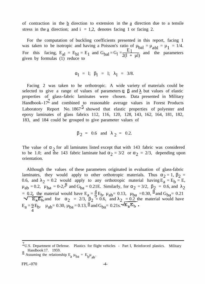
For the computation of buckling coefficients presented in this report, facing 1 was taken to be isotropic and having a Poisson's ratio of µbal = µabl = µ1 = 1/4. For this facing, Eal = Ebl = E1 and Gbal = Gl =
2(l E
+ l
µl) and the parameters given by formulas (1) reduce to
αl = l; βl = l; λl = 3/8.
Facing 2 was taken to be orthotropic. A wide variety of materials could be selected to give a range of values of parameters α β and λ but values of elastic properties of glass-fabric laminates were chosen. Data presented in Military Handbook-177 and combined to reasonable average values in Forest Products Laboratory Report No. 1867 5 showed that elastic properties of polyester and epoxy laminates of glass fabrics 112, 116, 120, 128, 143, 162, 164, 181, 182, 183, and 184 could be grouped to give parameter values of
β 2 = 0.6 and λ 2 = 0.2.
The value of α 2 for all laminates listed except that with 143 fabric was considered to be 1.0; and the 143 fabric laminate had α2 = 3/2 or α2 = 2/3, depending upon orientation.
Although the values of these parameters originated in evaluation of glass-fabric laminates, they would apply to other orthotropic materials. Thus α2 = 1, β2 = 0.6, and λ2 = 0.2 would apply to any orthotropic material having Ea = Eb = E, µab = 0.2, µ ba = 0-2, 8 and Gba = 0.21E. Similarly, for α2 = 3/2, β2 = 0.6, and λ2
4= 0.2, the material would have Ea = 9 Eb, µab and λ2 0.21s.
= 0.13, µba =0.30, 8 and Gba= 0.21 and for α2 = 2/3, β2 = 0.6, = 0.2 the material would have
Ea = 9 Eb, µab= 0.30, µba = 0.13, 8 and Gba= 4
7U.S. Department of Defense. Plastics for flight vehicles - Part I, Reinforced plastics. Military Handbook 17. 1959.8 Assuming the relationship Ea µba = Ebµ
ab.
FPL-070 -4-

Formulas
Load is applied to two opposite edges of the panel, as shown in figure 1. The length of these edges is b and the length of the other two edges is a. The load is applied at the neutral-axis of the panel so that the panel does not bend until the critical load is reached. It follows that the strains in the two facings are equal and the critical stress in each facing is given by
(2)
and
(3)
where N is the critical load of the sandwich panel in pounds per inch of edge, and t1 and t2 are, respectively, the thickness of the isotropic and the orthotropic facings. The parameter A is given by
(4)
where i = 1,2 denotes facing 1 or facing 2.
The buckling load of the sandwich, per unit panel width, N, is given by the formula 3
(5)
where b is length of the loaded edge of the panel; D is stiffness of spaced facings given by the formula
FPL-070 -5-

(6)
where h is the distance between facing centroids; D1 and D2 are stiffnesses of individual facings given by the formula
(7)
where i = 1,2, denotes facing 1 or facing 2; and coefficients KM K1 and K2 may be read from the curves presented; or calculated from the following formulas:
(8)
(9)
where
(10)
(11)
(12)
(13)
FPL-070 -6-
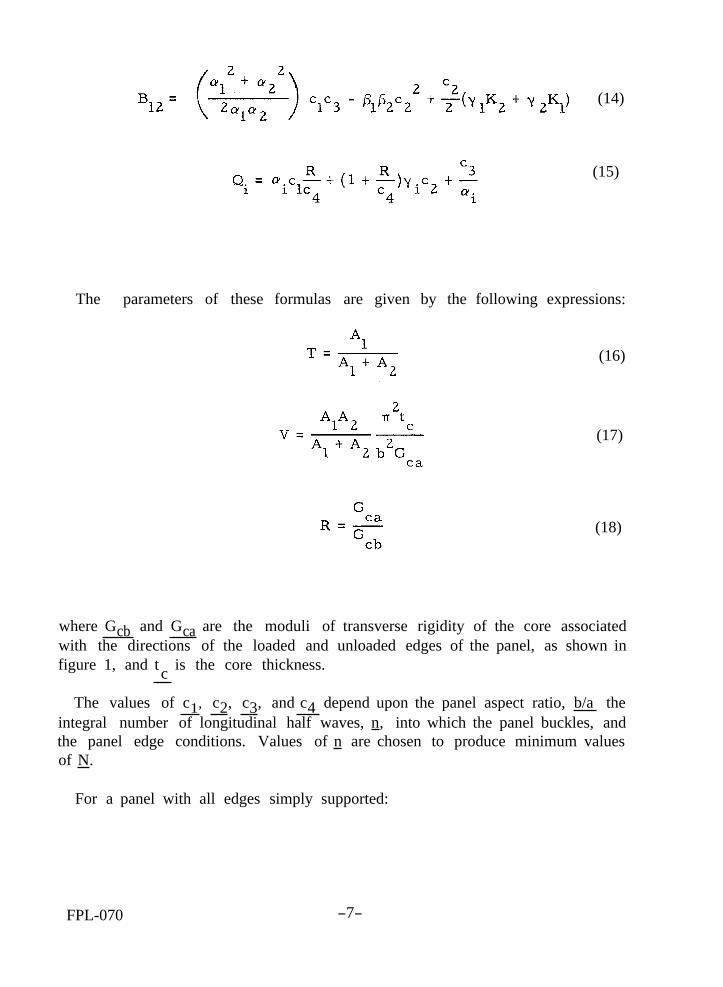
(14)
(15)
The parameters of these formulas are given by the following expressions:
(16)
(17)
(18)
where Gcb and Gca are the moduli of transverse rigidity of the core associated with the directions of the loaded and unloaded edges of the panel, as shown in figure 1, and t is the core thickness. c
The values of c1, c2, c3, and c4 depend upon the panel aspect ratio, b/a the integral number of longitudinal half waves, n, into which the panel buckles, and the panel edge conditions. Values of n are chosen to produce minimum values of N.
For a panel with all edges simply supported:
FPL-070 -7-

For a panel with loaded edges simply supported and other edges clamped:
For a panel with loaded edges clamped and other edges simply supported:
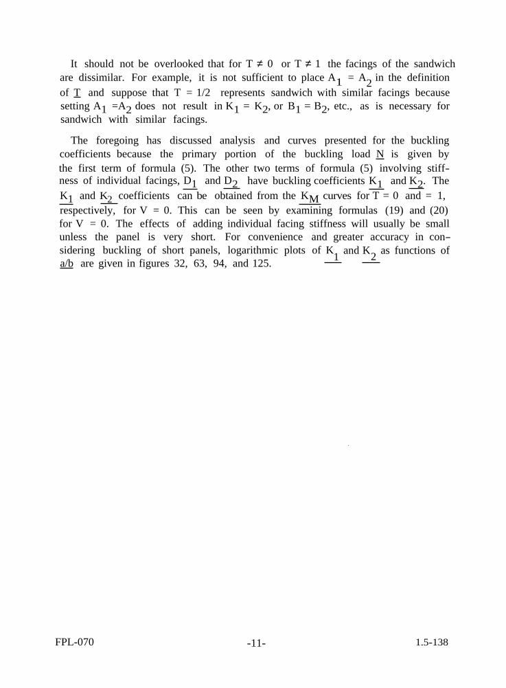
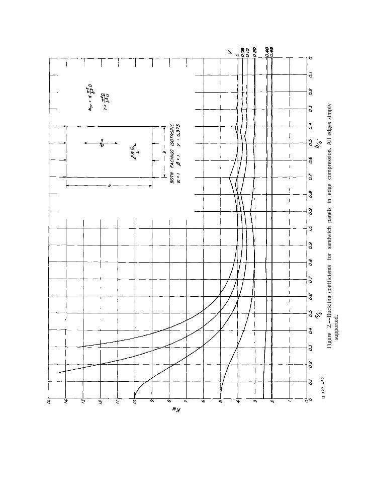
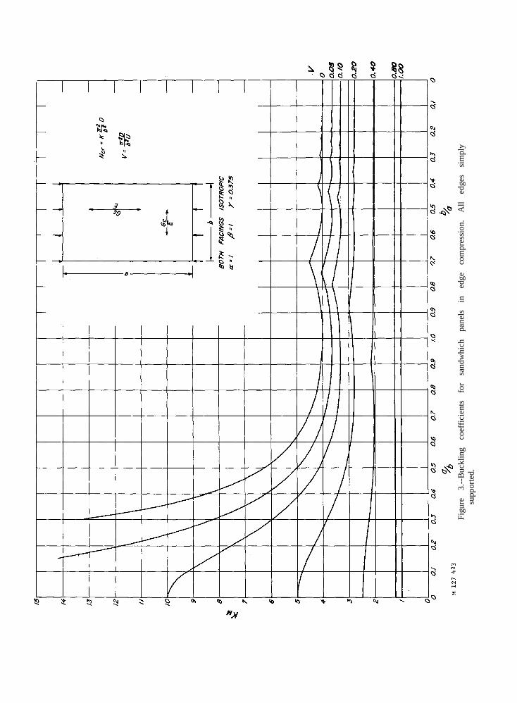
Discussion of Design Curves
Buckling coefficient curves for sandwich panels are presented in figures 2 to 125. The figures are divided into four main groups, depending on the type of support at the panel edges. Each group contains a set of curves for sandwich having both facings isotropic and three sets of curves for sandwich having dissimilar facings or both facings orthotropic, one set for each value of
FPL-070 -8-

the parameter α2 which differentiates between the three types of orthotropic glass-laminate facings.
The figures contain a family of curves consisting of a plot of KM against ab for various values of V. The families in each set of curves differ because they apply to different values of R. Each cusped curve is made up of portions of the curve for the n that gives the least value of K M The parameter a/b is used in the left half of the curve sheets, and the parameter b/a in the right half. Thus, values of KM for values of a/b from zero to infinity may be read.
Limits
1When a/b is zero, minimum values are given by KM = V. For other values of a/b, as the value of V increases, the value of KM decreases and the minimum points on the curve move to the left. There is a value of V for which the first minimum point of the curve occurs at a/b equal to zero, the KM intercept. This minimum point is common to the curves associated with all numbers of half waves. Of these curves, the curve for an infinite number of half waves yields the least critical value and is a horizontal straight line. These straight lines are shown on the curve sheets. If V is given a value equal to or greater than that
1associated with these straight lines, the critical value of KM is V . This is the "shear instability limit" of the critical load because substitution into formula
(5) results in N = h tc 2Gca for sandwich with facings so thin that D1 and D2 are
negligible. Thus, N is dependent upon core shear modulus, Gca and not upon elastic properties of facings.
Curves are provided for three values of the parameter R (0.4,1.0, and 2.5). Values of KM for other values of R may be estimated by reading from the curves the KM values for these three values of R and plotting them against R. The estimate may be made by reading the value of KM at the required value of R from a smooth curve sketched through the points. It should be noted that the curves for V equal to zero are, of course, independent of R. For convenience, these curves are duplicated in all three figures to which each applies.
The parameter T (formula (16)) was devised as a means of convenience in handling the analysis and presentation of results for sandwich with dissimilar facings. The role of T and its range of values can be understood most easily by examining its place in the parameters of the KM expression. T appears in the equations for ψ1, ψ2, and ψ3 (equations (10), (11), and (12)). If T = 0 is substituted into these equations, they become
FPL-070 -9-
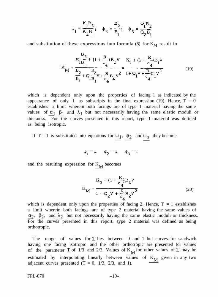
and substitution of these expressions into formula (8) for KM result in
(19)
which is dependent only upon the properties of facing 1 as indicated by the appearance of only 1 as subscripts in the final expression (19). Hence, T = 0 establishes a limit wherein both facings are of type 1 material having the same values of α1 β1 and λ1 but not necessarily having the same elastic moduli or thickness. For the curves presented in this report, type 1 material was defined as being isotropic.
If T = 1 is substituted into equations for ψ 1 , ψ 2 and ψ 3 they become
and the resulting expression for KM becomes
(20)
which is dependent only upon the properties of facing 2. Hence, T = 1 establishes a limit wherein both facings are of type 2 material having the same values of α2, β2, and λ2 but not necessarily having the same elastic moduli or thickness. For the curves presented in this report, type 2 material was defined as being orthotropic.
The range of values for T lies between 0 and 1 but curves for sandwich having one facing isotropic and the other orthotropic are presented for values of the parameter T of 1/3 and 2/3. Values of K M for other values of T may be
estimated by interpolating linearly between values of KM given in any two adjacent curves presented (T = 0, 1/3, 2/3, and 1).
FPL-070 -10-
It should not be overlooked that for T ≠ 0 or T ≠ 1 the facings of the sandwich are dissimilar. For example, it is not sufficient to place A1 = A2 in the definition of T and suppose that T = 1/2 represents sandwich with similar facings because setting A1 =A2 does not result in K1 = K2, or B1 = B2, etc., as is necessary for sandwich with similar facings.
The foregoing has discussed analysis and curves presented for the buckling coefficients because the primary portion of the buckling load N is given by the first term of formula (5). The other two terms of formula (5) involving stiffness of individual facings, D1 and D2 have buckling coefficients K1 and K2. The K1 and K2 coefficients can be obtained from the KM curves for T = 0 and = 1, respectively, for V = 0. This can be seen by examining formulas (19) and (20) for V = 0. The effects of adding individual facing stiffness will usually be small unless the panel is very short. For convenience and greater accuracy in considering buckling of short panels, logarithmic plots of K1 and K2 as functions of a/b are given in figures 32, 63, 94, and 125.
FPL-070 -11- 1.5-138

Figure 1.--Notation for dimensions and elastic properties of sandwich panel.
Figu
re
2.--
Buc
klin
g co
effic
ient
s fo
r sa
ndw
ich
pane
ls
in e
dge
com
pres
sion
. A
ll ed
ges
sim
ply
supp
orte
d.
Figu
re
3.--
Buc
klin
g co
effic
ient
s fo
r sa
ndw
hich
pa
nels
in
ed
ge
com
pres
sion
. A
ll ed
ges
sim
ply
supp
orte
d.
M 127 424
Figu
re
4.--
Buc
klin
g co
effic
ient
s fo
r sa
ndw
ich
pane
ls
in
edge
co
mpr
essi
on.
All
edge
s si
mpl
y su
ppor
ted.

Figu
re 5
.--B
uckl
ing
coef
ficie
nts
for
sand
wic
h pa
nels
in
edge
com
pres
sion
. All
edge
s si
mpl
y su
ppor
ted.
M127 426
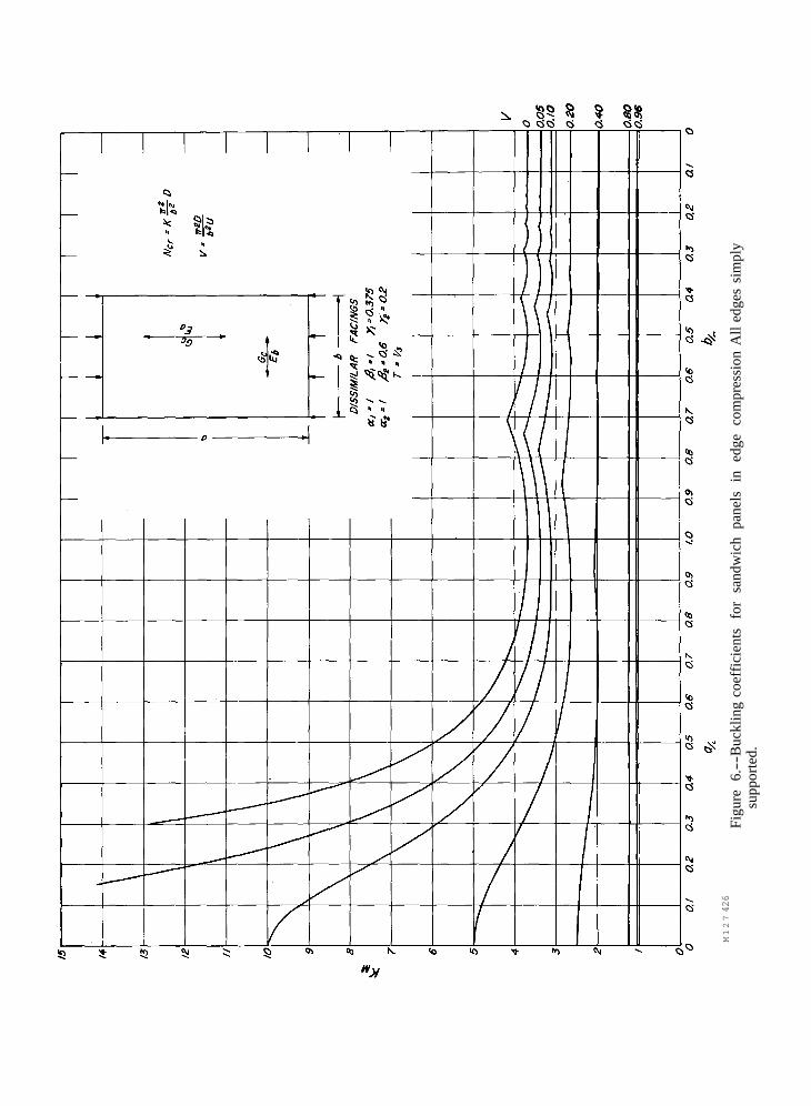
Figu
re 6
.--B
uckl
ing
coef
ficie
nts
for
sand
wic
h pa
nels
in
edge
com
pres
sion
All
edge
s si
mpl
y su
ppor
ted.
M 127 431
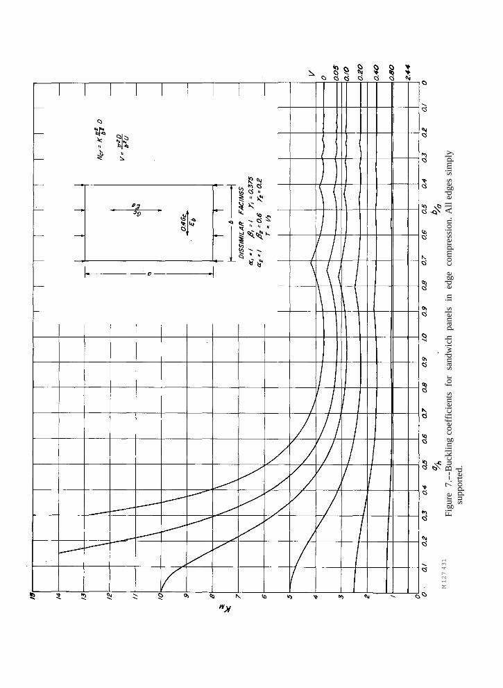
Fi
gure
7.-
-Buc
klin
g co
effic
ient
s fo
r sa
ndw
ich
pane
ls i
n ed
ge c
ompr
essi
on. A
ll ed
ges
sim
ply
supp
orte
d.

Figu
re
8.--
Buc
klin
g co
effic
ient
s fo
r sa
ndw
ich
pane
ls i
n ed
ge c
ompr
essi
on. A
ll ed
ges
sim
ply
supp
orte
d.

Figu
re 9
.--B
uckl
ing
coef
ficie
nts
for
sand
wic
h pa
nels
in
edge
com
pres
sion
. All
edge
s si
mpl
y su
ppor
ted.
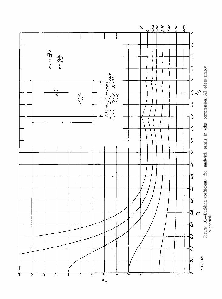
Figu
re
10.-
-Buc
klin
g co
effic
ient
s fo
r sa
ndw
ich
pane
ls
in
edge
co
mpr
essi
on.
All
edge
s si
mpl
y su
ppor
ted.

Figu
re 1
1.--
Buc
klin
g co
effic
ient
s fo
r sa
ndw
ich
pane
ls i
n ed
ge c
ompr
essi
on. A
ll ed
ges
sim
ply
supp
orte
d.
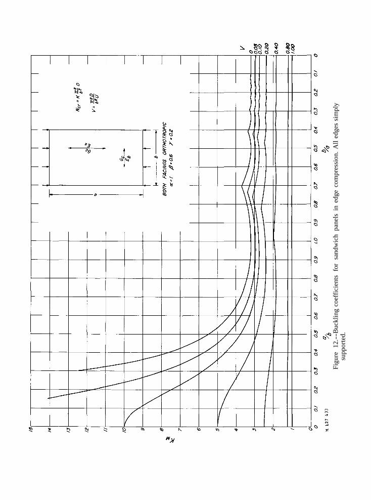
Figu
re 1
2.--
Buc
klin
g co
effic
ient
s fo
r sa
ndw
ich
pane
ls i
n ed
ge c
ompr
essi
on. A
ll ed
ges
sim
ply
supp
orte
d.

Figu
re
13.-
-Buc
klin
g co
effic
ient
s fo
r sa
ndw
ich
pane
ls
in
edge
co
mpr
essi
on.
All
edge
s si
mpl
y su
ppor
ted.
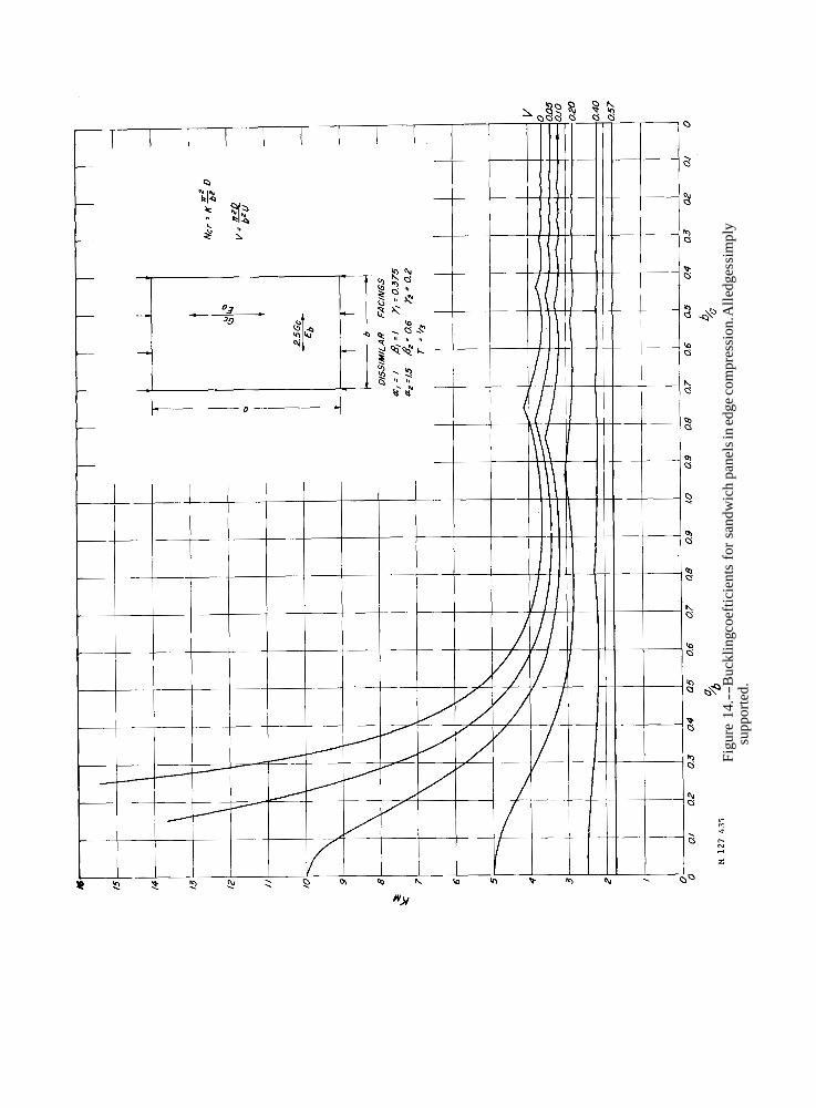
Figu
re 1
4.--
Buc
klin
gcoe
ftici
ents
for
san
dwic
h pa
nels
in ed
ge co
mpr
essi
on.A
lledg
essi
mpl
y su
ppor
ted.

Figu
re 1
5.--
Buc
klin
g co
effic
ient
s fo
r sa
ndw
ich
pane
ls in
edg
e co
mpr
essi
on. A
ll ed
ges s
impl
y su
ppor
ted.
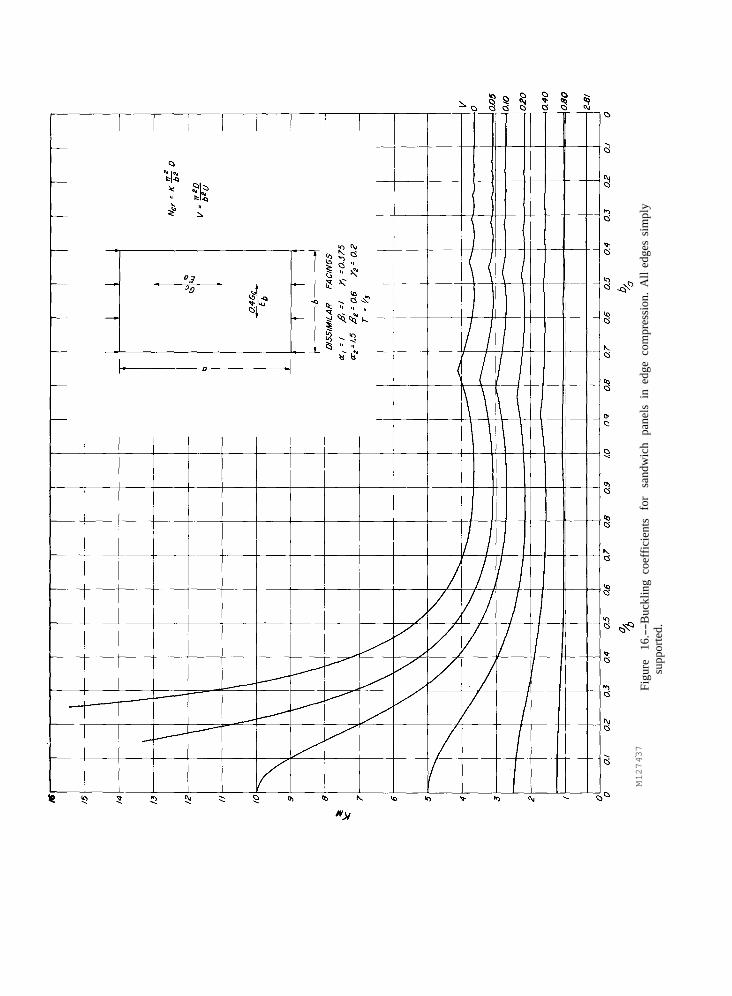
M127437
Figu
re
16.-
-Buc
klin
g co
effic
ient
s fo
r sa
ndw
ich
pane
ls i
n ed
ge c
ompr
essi
on.
All
edge
s si
mpl
y su
ppor
ted.

M 127 438
Figu
re
17.-
-Buc
klin
g co
effic
ient
s fo
r sa
ndw
ich
pane
ls
in
edge
co
mpr
essi
on.
All
edge
s si
mpl
y su
ppor
ted.

Figu
re
18. -
-Buc
klin
g co
effic
ient
s fo
r sa
ndw
ich
pane
ls i
n ed
ge c
ompr
essi
on.
All
edge
s si
mpl
y su
ppor
ted.
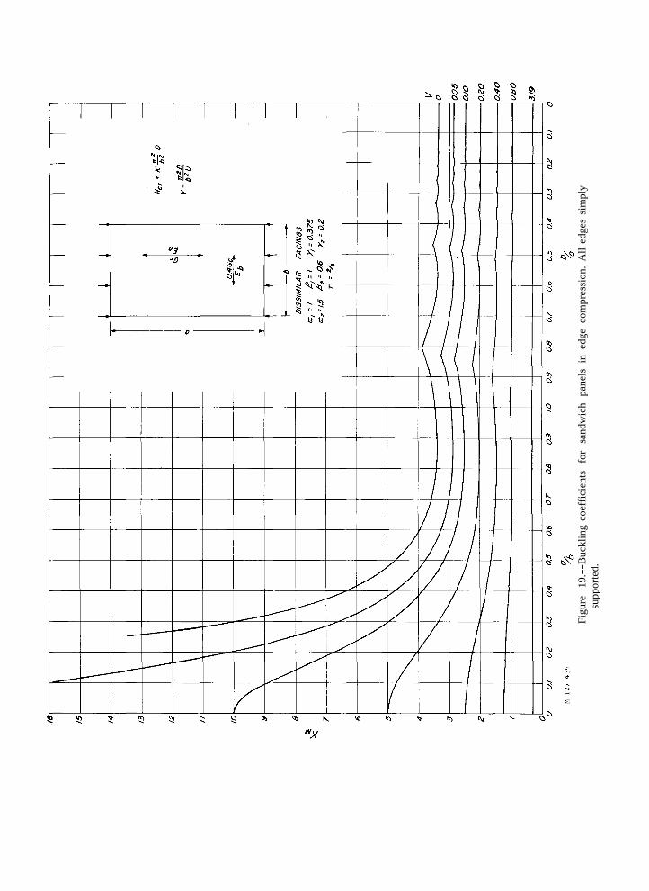
Figu
re
19.-
-Buc
klin
g co
effic
ient
s fo
r sa
ndw
ich
pane
ls i
n ed
ge c
ompr
essi
on.
All
edge
s si
mpl
y su
ppor
ted.
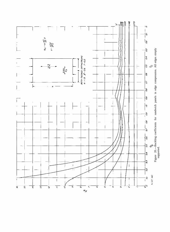
Figu
re
20.--B
uckl
ing
coef
ficie
nts
for
sand
wic
h pa
nels
in
edge
com
pres
sion
. A
ll ed
ges
sim
ply
supp
orte
d.

Figu
re
21.-
-Buc
klin
g co
effic
ient
s fo
r sa
ndw
ich
pane
ls i
n ed
ge c
ompr
essi
on. A
ll ed
ges
sim
ply
supp
orte
d.
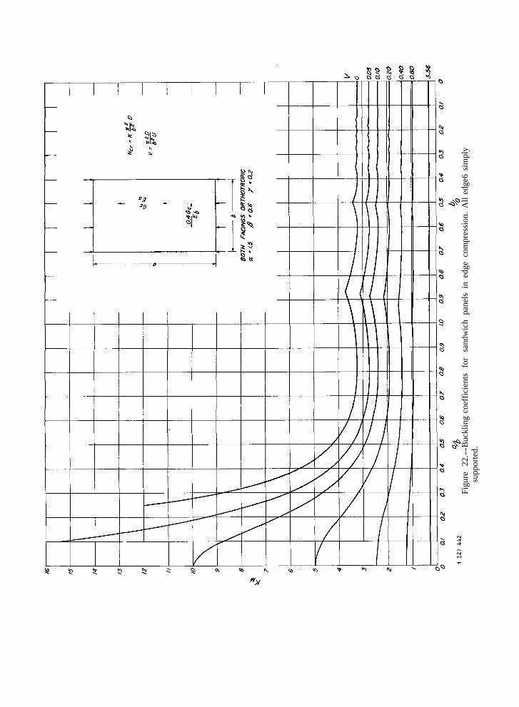
Figu
re
22.-
-Buc
klin
g co
effic
ient
s fo
r sa
ndw
ich
pane
ls i
n ed
ge c
ompr
essi
on.
All
edge
6 si
mpl
y su
ppor
ted.
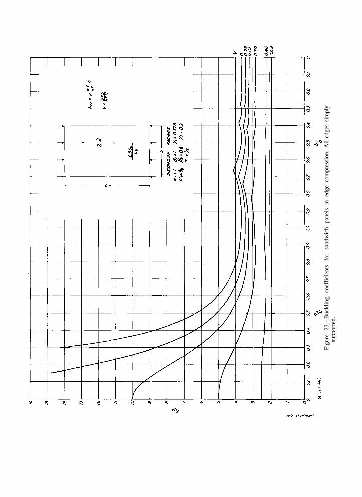
Figu
re
23.--
Buc
klin
g co
effic
ient
s fo
r sa
ndw
ich
pane
ls i
n ed
ge c
ompr
essi
on.
All
edge
s si
mpl
y su
ppor
ted.
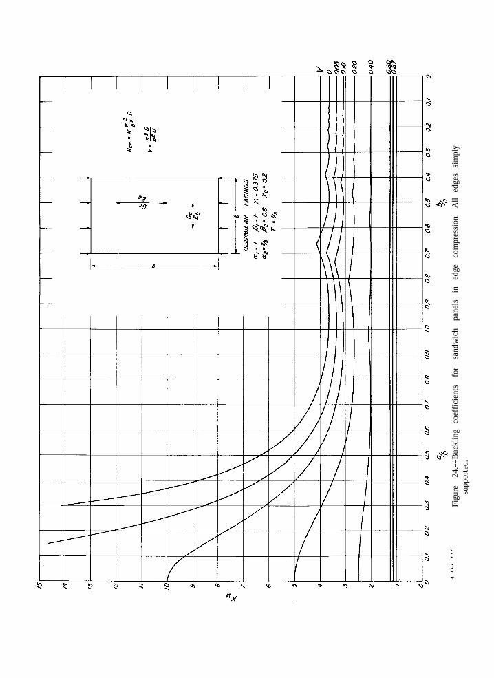
Figu
re
24.--B
uckl
ing
coef
ficie
nts
for
sand
wic
h pa
nels
in
ed
ge
com
pres
sion
. A
ll ed
ges
sim
ply
supp
orte
d.
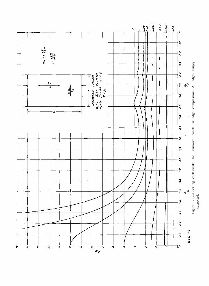
Figu
re
25.-
-Buc
klin
g co
effic
ient
s fo
r sa
ndw
ich
pane
ls
in
edge
co
mpr
essi
on.
All
edge
s si
mpl
y su
ppor
ted.
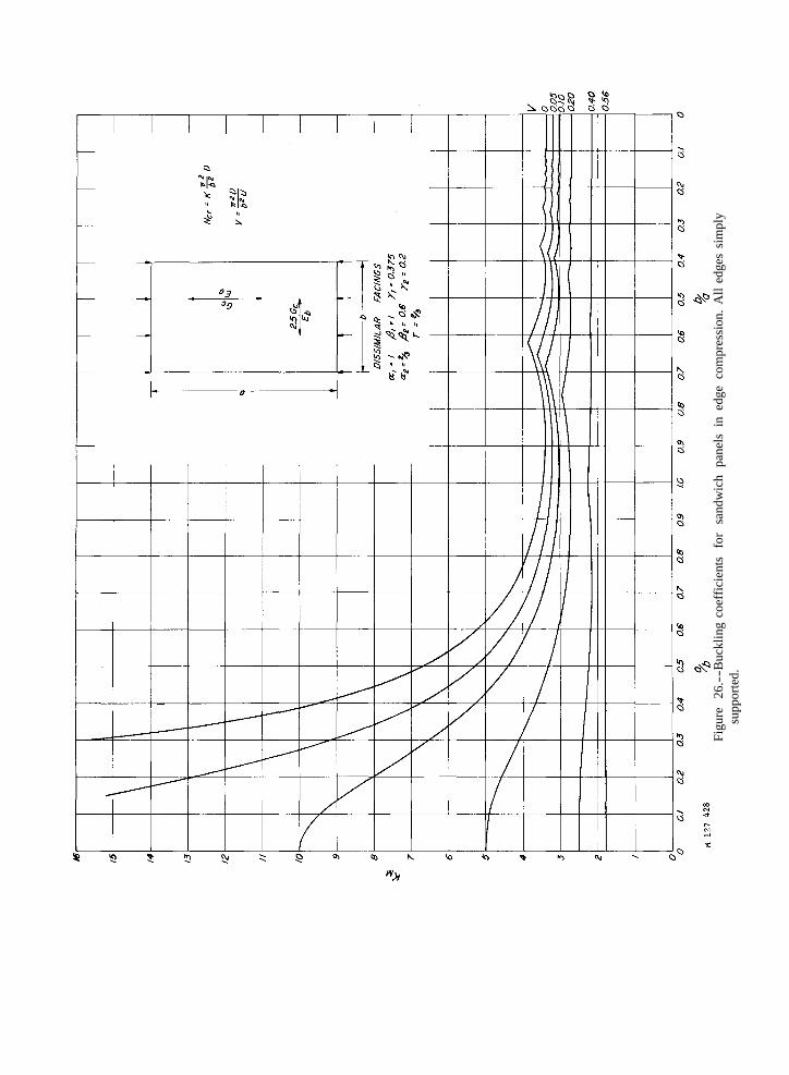
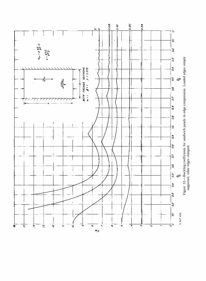
Figu
re
26.--B
uckl
ing
coef
ficie
nts
for
sand
wic
h pa
nels
in
edge
com
pres
sion
. A
ll ed
ges
sim
ply
supp
orte
d.

Figu
re
27.--B
uckl
ing
coef
ficie
nts
for
sand
wic
h pa
nels
in
edge
com
pres
sion
, A
ll ed
ges
sim
ply
supp
orte
d.

Figu
re
28.-
-Buc
klin
g co
effic
ient
s fo
r sa
ndw
ich
pane
ls i
n ed
ge c
ompr
essi
on.
All
edge
s si
mpl
y su
ppor
ted.

Figu
re
29.-
-Buc
klin
g co
effic
ient
s fo
r sa
ndw
ich
pane
ls i
n ed
ge c
ompr
essi
on.
All
edge
s si
mpl
y su
ppor
ted
Figu
re
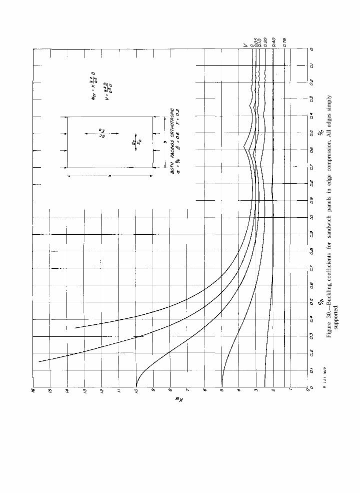
30.-
-Buc
klin
g co
effic
ient
s fo
r sa
ndw
ich
pane
ls i
n ed
ge c
ompr
essi
on.
All
edge
s si
mpl
y su
ppor
ted.

Figu
re
31.-
-Buc
klin
g co
effic
ient
s fo
r sa
ndw
ich
pane
ls i
n ed
ge c
ompr
essi
on.
All
edge
s si
mpl
y su
ppor
ted.
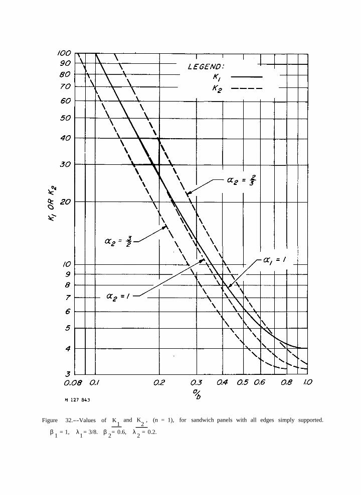
Figure 32.--Values of K1
and K2
, (n = 1), for sandwich panels with all edges simply supported.
β 1 = 1, λ 1 = 3/8. β 2 = 0.6, λ 2 = 0.2.
Figu
re 3
3.--
Buc
klin
g co
effic
ient
s fo
r sa
ndw
ich
pane
ls i
n ed
ge c
ompr
essi
on.
Load
ed e
dges
sim
ply
supp
orte
d, o
ther
edg
es c
lam
ped.
Figu
re 3
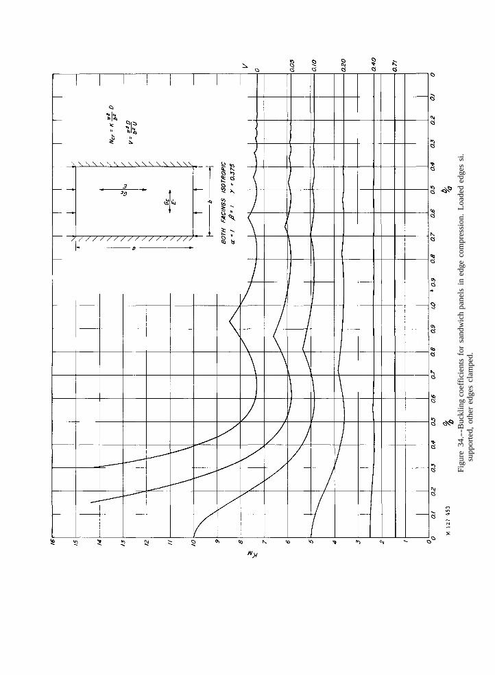
4.--
Buc
klin
g co
effic
ient
s fo
r sa
ndw
ich
pane
ls i
n ed
ge c
ompr
essi
on.
Load
ed e
dges
si.
supp
orte
d, o
ther
edg
es c
lam
ped.
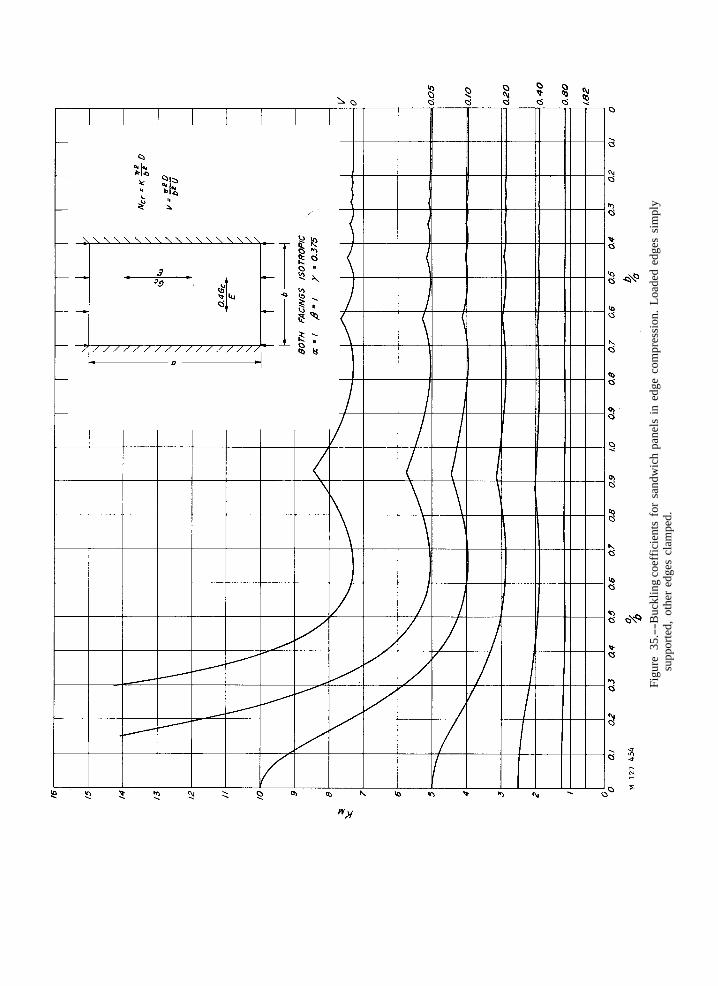
Figu
re 3
5.--
Buc
klin
g co
effic
ient
s fo
r sa
ndw
ich
pane
ls i
n ed
ge c
ompr
essi
on.
Load
ed e
dges
sim
ply
supp
orte
d, o
ther
edg
es c
lam
ped.
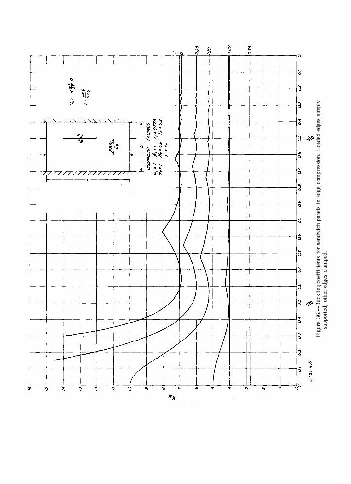
Figu
re 3
6.--
Buc
klin
g co
effic
ient
s fo
r sa
ndw
ich
pane
ls i
n ed
ge c
ompr
essi
on.
Load
ed e
dges
sim
ply
supp
orte
d, o
ther
edg
es c
lam
ped.
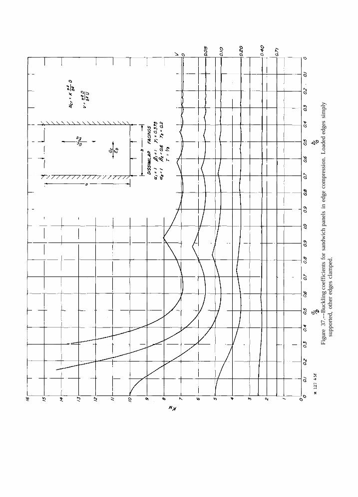
Figu
re 3
7.--
Buc
klin
g co
effic
ient
s fo
r sa
ndw
ich
pane
ls i
n ed
ge c
ompr
essi
on.
Load
ed e
dges
sim
ply
supp
orte
d, o
ther
edg
es c
lam
ped.
Figu
re 3
8.--
Buc
klin
g co
effic
ient
s fo
r sa
ndw
ich
pane
ls i
n ed
ge c
ompr
essi
on.
Load
ed e
dges
sim
ply
supp
orte
d, o
ther
edg
es c
lam
ped.

Figu
re 3
9.--
Buc
klin
g co
effic
ient
s fo
r sa
ndw
ich
pane
ls i
n ed
ge c
ompr
essi
on.
Load
ed e
dges
sim
ply
supp
orte
d, o
ther
edg
es c
lam
ped.
Figu
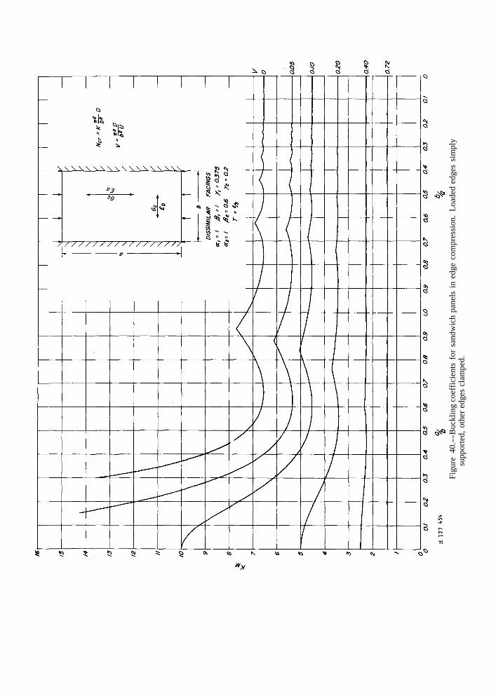
re 4
0.--
Buc
klin
g co
effic
ient
s fo
r sa
ndw
ich
pane
ls i
n ed
ge c
ompr
essi
on.
Load
ed e
dges
sim
ply
supp
orte
d, o
ther
edg
es c
lam
ped.

Figu
re 4
1.--
Buc
klin
g co
effic
ient
s fo
r sa
ndw
ich
pane
ls i
n ed
ge c
ompr
essi
on.
Load
ed e
dges
sim
ply
supp
orte
d, o
ther
edg
es c
lam
ped.
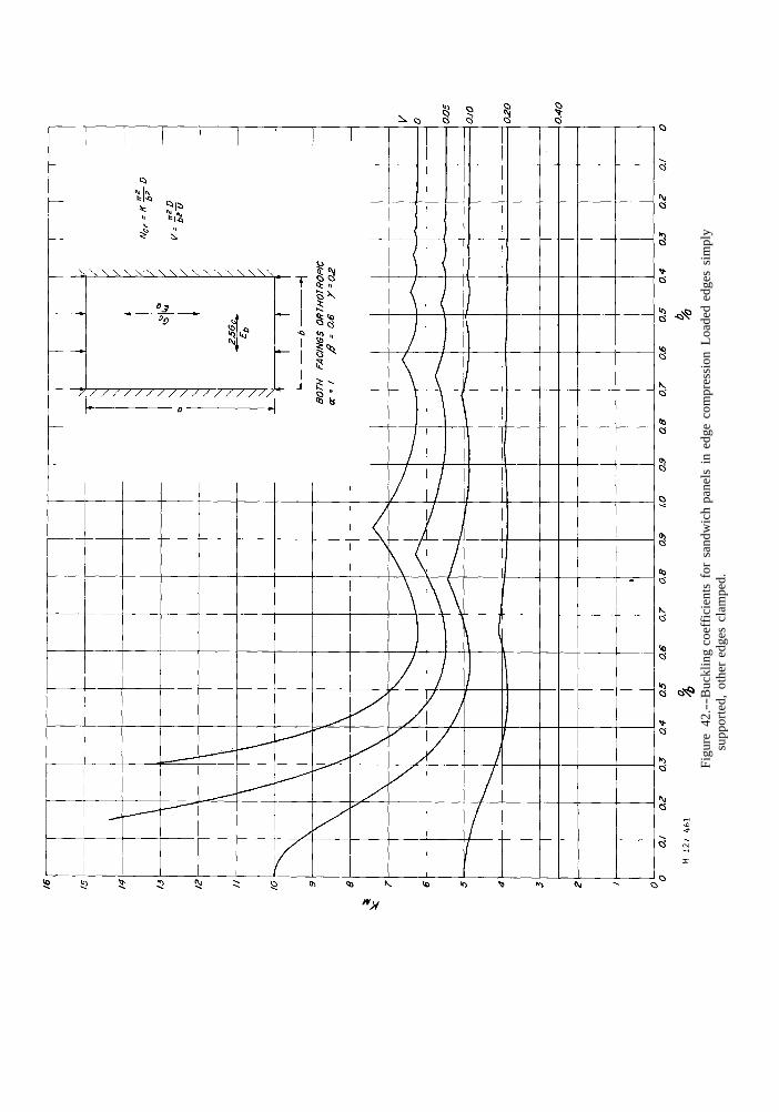
Figu
re 4
2.--
Buc
klin
g co
effic
ient
s fo
r sa
ndw
ich
pane
ls i
n ed
ge c
ompr
essi
on L
oade
d ed
ges
sim
ply
supp
orte
d, o
ther
edg
es c
lam
ped.
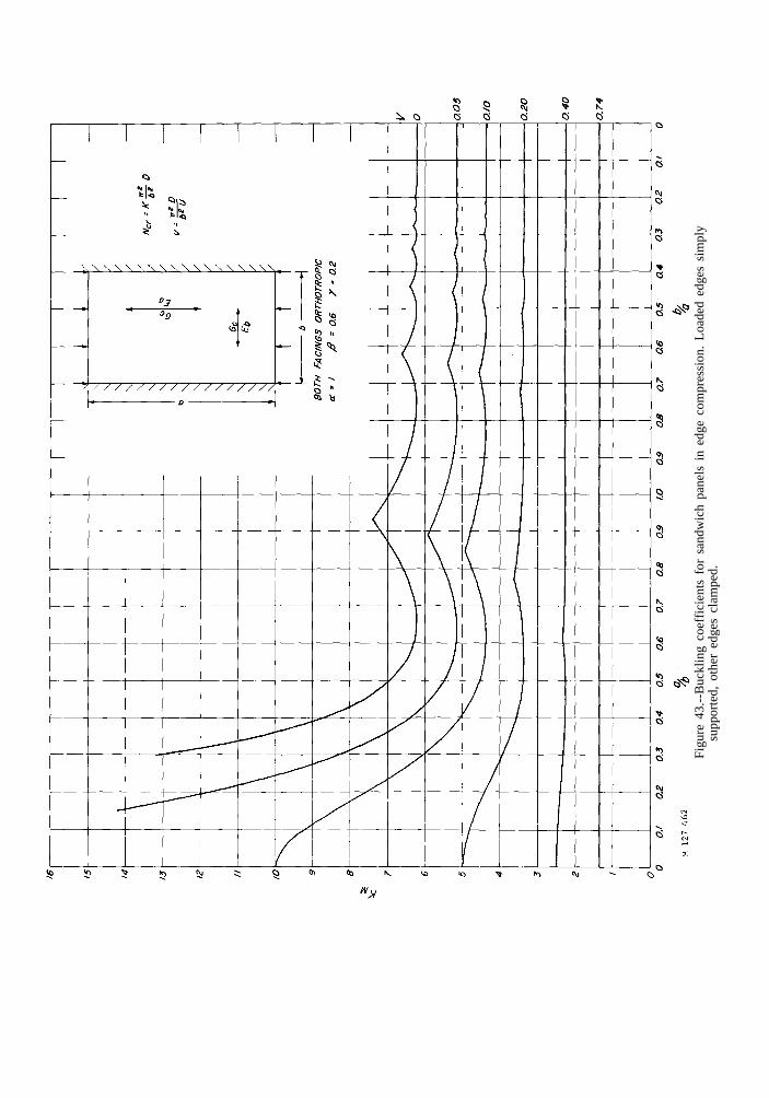
Figu
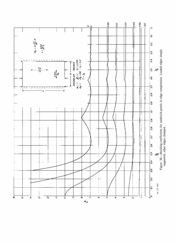
re 4
3.--
Buc
klin
g co
effic
ient
s fo
r sa
ndw
ich
pane
ls i
n ed
ge c
ompr
essi
on.
Load
ed e
dges
sim
ply
supp
orte
d, o
ther
edg
es c
lam
ped.

Figu
re 4
4.--
Buc
klin
g coe
ffic
ient
s fo
r sa
ndw
ich
pane
ls i
n ed
ge c
ompr
essi
on.
Load
ed e
dges
sim
ply
supp
orte
d, o
ther
edg
es c
lam
ped.
Figu
re 4
5.--
Buc
klin
g co
effic
ient
s fo
r sa
ndw
ich
pane
ls i
n ed
ge c
ompr
essi
on.
Load
ed e
dges
sim
ply
supp
orte
d, o
ther
edg
es c
lam
ped.

Figu
re 4
6.--
Buc
klin
g co
effic
ient
s fo
r sa
ndw
ich
pane
ls i
n ed
ge c
ompr
essi
on.
Load
ed e
dges
sim
ply
supp
orte
d, o
ther
edg
es c
lam
ped.

Figu
re 4
7. --
Buc
klin
g co
effic
ient
s fo
r sa
ndw
ich
pane
ls in
edg
e co
mpr
essi
on.
Load
ed e
dges
sim
ply
supp
orte
d, o
ther
edg
es c
lam
ped.
Figu
re 4
8.--
Buc
klin
g co
effic
ient
s fo
r sa
ndw
ich
pane
ls i
n ed
ge c
ompr
essi
on.
Load
ed e
dges
sim
ply
supp
orte
d, o
ther
edg
es c
lam
ped.
Figu
re 4
9.--
Buc
klin
g co
effic
ient
s fo
r sa
ndw
ich
pane
ls i
n ed
ge c
ompr
essi
on.
Load
ed e
dges
sim
ply
supp
orte
d, o
ther
edg
es c
lam
ped.

Figu
re 5
0.--
Buc
klin
g co
effic
ient
s fo
r sa
ndw
ich
pane
ls i
n ed
ge c
ompr
essi
on.
Load
ed e
dges
sim
ply
supp
orte
d, o
ther
edg
es c
lam
ped.
Figu
re 5
1. --
Buc
klin
g co
effic
ient
s fo
r sa
ndw
ich
pane
ls i
n ed
ge c
ompr
essi
on. L
oade
d ed
ges
sim
ply
supp
orte
d, o
ther
edg
es c
lam
ped.

Figu
re 5
2.--
Buc
klin
g co
effic
ient
s fo
r sa
ndw
ich
pane
ls i
n ed
ge c
ompr
essi
on.
Load
ed e
dges
sim
ply
supp
orte
d, o
ther
edg
es c
lam
ped.
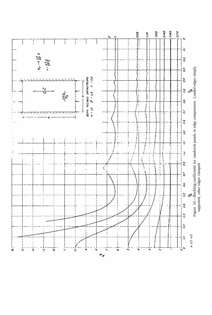
Figu
re 5
3.--
Buc
klin
g co
effic
ient
s fo
r sa
ndw
ich
pane
ls i
n ed
ge c
ompr
essi
on.
Load
ed e
dges
sim
ply
supp
orte
d, o
ther
edg
es c
lam
ped.

Figu
re 5
4.--
Buc
klin
g co
effic
ient
s fo
r sa
ndw
ich
pane
ls in
edg
e co
mpr
essi
on.
Load
ed e
dges
sim
ply
supp
orte
d, o
ther
edg
es c
lam
ped.

Figu
re 5
5.--
Buc
klin
g co
effic
ient
s fo
r sa
ndw
ich
pane
ls i
n ed
ge c
ompr
essi
on.
Load
ed e
dges
sim
ply
supp
orte
d, o
ther
edg
es c
lam
ped.

Figu
re 5
6.--
Buc
klin
g co
effic
ient
s fo
r sa
ndw
ich
pane
ls i
n ed
ge c
ompr
essi
on.
Load
ed e
dges
sim
ply
supp
orte
d, o
ther
edg
es c
lam
ped.
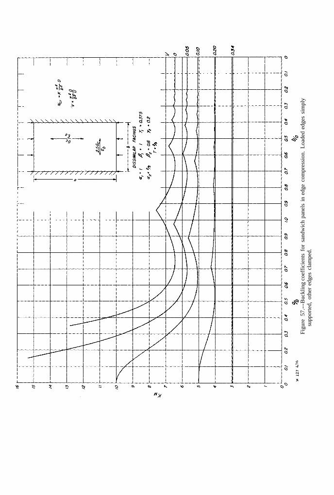
Figu
re 5
7.--
Buc
klin
g co
effic
ient
s fo
r sa
ndw
ich
pane
ls i
n ed
ge c
ompr
essi
on.
Load
ed e
dges
sim
ply
supp
orte
d, o
ther
edg
es c
lam
ped.

Figu
re 5
8.--
Buc
klin
g co
effic
ient
s fo
r sa
ndw
ich
pane
ls i
n ed
ge c
ompr
essi
on.
Load
ed e
dges
sim
ply
supp
orte
d, o
ther
edg
es c
lam
ped.
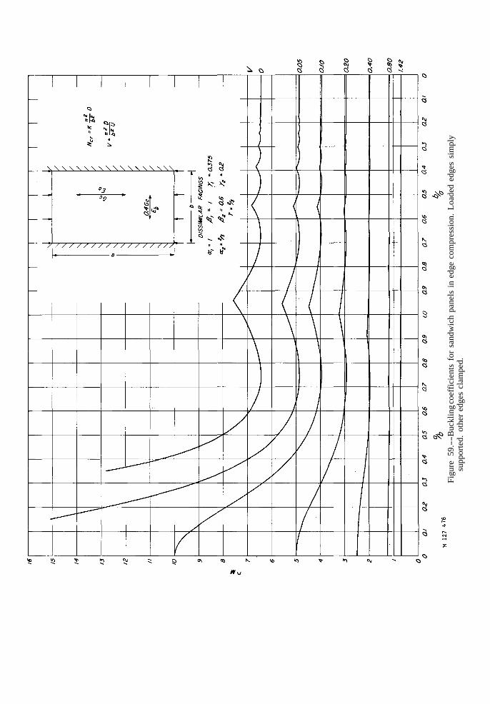
Figu
re 5
9.--
Buc
klin
g co
effic
ient
s fo
r sa
ndw
ich
pane
ls i
n ed
ge c
ompr
essi
on.
Load
ed e
dges
sim
ply
supp
orte
d. o
ther
edg
es c
lam
ped.

Figu
re 6
0.--
Buc
klin
g co
effic
ient
s fo
r sa
ndw
ich
pane
ls i
n ed
ge c
ompr
essi
on.
Load
ed e
dges
sim
ply
supp
orte
d, o
ther
edg
es c
lam
ped.
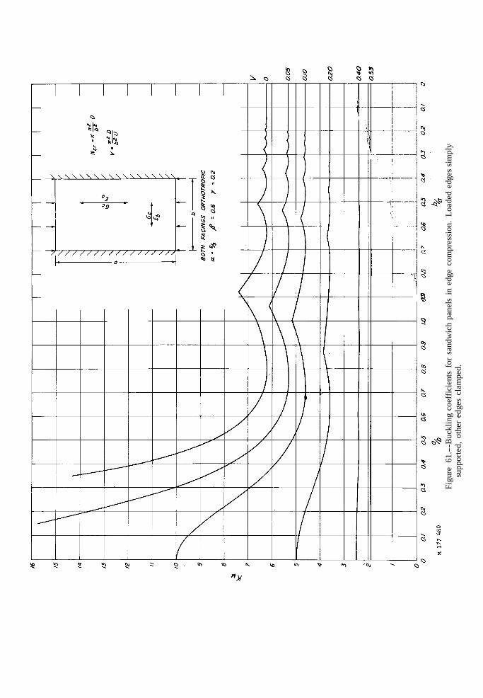
Figu
re 6
1.--
Buc
klin
g co
effic
ient
s fo
r sa
ndw
ich
pane
ls i
n ed
ge c
ompr
essi
on.
Load
ed e
dges
sim
ply
supp
orte
d, o
ther
edg
es c
lam
ped.

Figu
re 6
2.--
Buc
klin
g co
effic
ient
s fo
r sa
ndw
ich
pane
ls i
n ed
ge c
ompr
essi
on.
Load
ed e
dge
sim
ply
supp
orte
d, o
ther
edg
es c
lam
ped.

Figure 63.--Values of K1
and K2
, (n = 1), for sandwich panels with loaded edges simply supported,
other edges clamped, β1= 1, λ 1 = 3/8. β 2 = 0.6, λ
2 = 0.2.
Figu
re 6
4.--
Buc
klin
g coe
ffic
ient
s fo
r sa
ndw
ich
pane
ls in
edge
com
pres
sion
. Lo
aded
edg
es c
lam
ped,
ot
her
edge
s si
mpl
y su
ppor
ted.

Figu
re 6
5.--
Buc
klin
g co
effic
ient
s fo
r sa
ndw
ich
pane
ls i
n ed
ge c
ompr
essi
on.
Load
ed e
dges
cla
mpe
d,
othe
r ed
ges
sim
ply
supp
orte
d.
Figu
re 6
6.--
Buc
klin
gcoe
ffic
ient
s fo
r sa
ndw
ich
pane
ls in
edge
com
pres
sion
. Lo
aded
edg
es c
lam
ped,
ot
her
edge
s si
mpl
y su
ppor
ted.

Figu
re 6
7.--
Buc
klin
gcoe
ffic
ient
s fo
r sa
ndw
ich
pane
ls in
edg
e co
mpr
essi
on.
Load
ed e
dges
cla
mpe
d,
othe
r ed
ges
sim
ply
supp
orte
d.

Figu
re 6
8.--
Buc
klin
gcoe
ffic
ient
s fo
r sa
ndw
ich
pane
ls in
edg
e co
mpr
essi
on.
Load
ed e
dges
cla
mpe
d,
othe
r ed
ges
sim
ply
supp
orte
d.
Figu
re 6
9.--
Buc
klin
g co
effic
ient
s fo
r sa
ndw
ich
pane
ls i
n ed
ge c
ompr
essi
on. L
oade
d ed
ges
clam
ped,
ot
her
edge
s si
mpl
y su
ppor
ted.

Figu
re 7
0.--
Buc
klin
gcoe
ffic
ient
s fo
r sa
ndw
ich
pane
ls in
edge
com
pres
sion
. Lo
aded
edg
es c
lam
ped,
ot
her
edge
s si
mpl
y su
ppor
ted.
Figu
re 7
1.--
Buc
klin
gcoe
ffic
ient
s fo
r sa
ndw
ich
pane
ls in
edg
e co
mpr
essi
on.
Load
ed e
dges
cla
mpe
d,
othe
r ed
ges
sim
ply
supp
orte
d.
Figu
re 7
2.--
Buc
klin
gcoe
ffic
ient
s fo
r sa
ndw
ich
pane
ls in
edge
com
pres
sion
. Lo
aded
edg
es c
lam
ped,
ot
her e
dges
sim
ply
supp
orte
d.

Figu
re 7
3.--
Buc
klin
gcoe
ffic
ient
s fo
r sa
ndw
ich
pane
ls in
edg
e co
mpr
essi
on.
Load
ed e
dges
cla
mpe
d,
othe
r ed
ges
sim
ply
supp
orte
d.
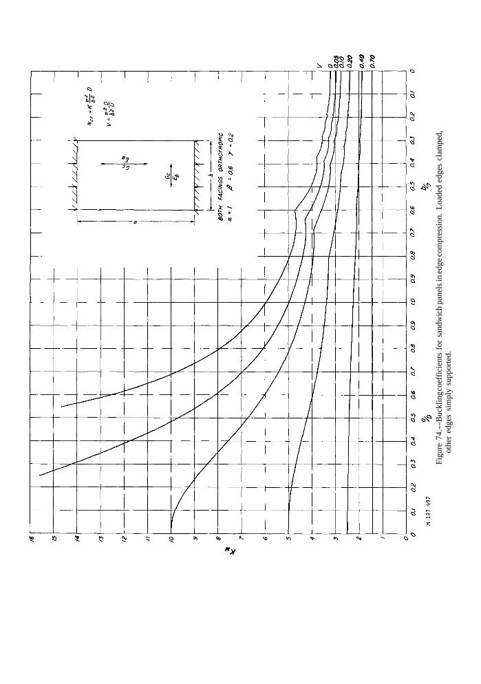
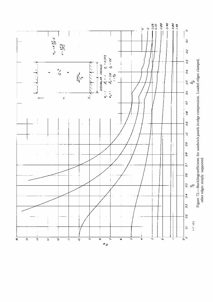
Figu
re 7
4.--
Buc
klin
gcoe
ffic
ient
s fo
r sa
ndw
ich
pane
ls in
edge
com
pres
sion
. Lo
aded
edg
es c
lam
ped,
ot
her
edge
s si
mpl
y su
ppor
ted.
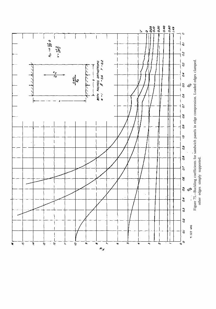
Figu
re 7
5.--
Buc
klin
g co
effic
ient
s fo
r sa
ndw
ich
pane
ls in
edg
e co
mpr
essi
on. L
oade
d ed
ges
clam
ped.
ot
her
edge
s si
mpl
y su
ppor
ted.
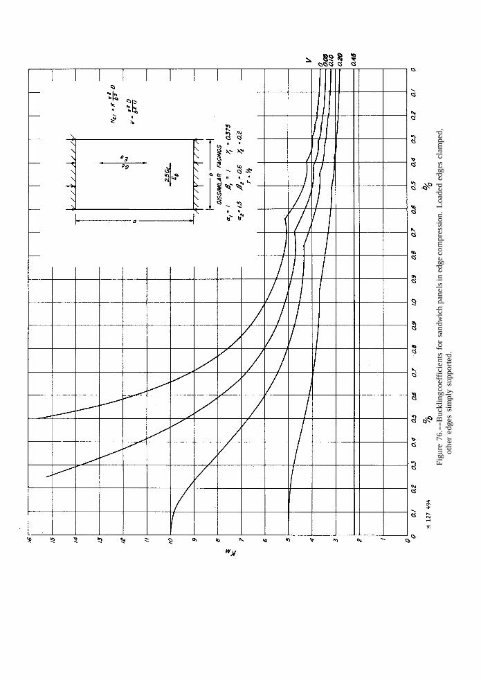
Figu
re 7
6.--
Buc
klin
gcoe
ffic
ient
s fo
r sa
ndw
ich
pane
ls in
edg
e co
mpr
essi
on.
Load
ed e
dges
cla
mpe
d,
othe
r ed
ges
sim
ply
supp
orte
d.

Figu
re 7
7.--
Buc
klin
gcoe
ffic
ient
s fo
r sa
ndw
ich
pane
ls in
edge
com
pres
sion
. Lo
aded
edg
es c
lam
ped,
ot
her
edge
s si
mpl
y su
ppor
ted.
Figu
re 7
8.--
Buc
klin
gcoe
ffic
ient
s fo
r sa
ndw
ich
pane
ls i
n ed
ge co
mpr
essi
on.
Load
ed e
dges
cla
mpe
d,
othe
r ed
ges
sim
ply
supp
orte
d.

Figu
re 7
9.--
Buc
klin
g co
effic
ient
s fo
r sa
ndw
ich
pane
ls in
edg
e co
mpr
essi
on.
Load
ed e
dges
cla
mpe
d,
othe
r ed
ges
sim
ply
supp
orte
d.
Figu
re 8
0.--
Buc
klin
gcoe
ffic
ient
s fo
r sa
ndw
ich
pane
ls in
edge
com
pres
sion
. Lo
aded
edg
es c
lam
ped,
ot
her
edge
s si
mpl
y su
ppor
ted.

Figu
re 8
1.--
Buc
klin
gcoe
ffic
ient
s fo
r sa
ndw
ich
pane
ls in
edg
e co
mpr
essi
on.
Load
ed e
dges
cla
mpe
d,
othe
r ed
ges
sim
ply
supp
orte
d.

Figu
re 8
2.--
Buc
klin
gcoe
ffic
ient
s fo
r sa
ndw
ich
pane
ls in
edge
com
pres
sion
. Lo
aded
edg
es c
lam
ped,
ot
her
edge
s si
mpl
y su
ppor
ted.
Figu
re 8
3.--
Buc
klin
gcoe
ffic
ient
s fo
r sa
ndw
ich
pane
ls in
edg
e co
mpr
essi
on.
Load
ed e
dges
cla
mpe
d,
othe
r ed
ges
sim
ply
supp
orte
d.

Figu
re 8
4.--
Buc
klin
g coe
ffic
ient
s fo
r san
dwic
h pa
nels
in e
dge
com
pres
sion
. Lo
aded
edg
es c
lam
ped,
ot
her
edge
s si
mpl
y su
ppor
ted.

Figu
re 8
5.--
Buc
klin
g coe
ffic
ient
s fo
r sa
ndw
ich
pane
ls in
edg
e co
mpr
essi
on.
Load
ed e
dges
cla
mpe
d,
othe
r ed
ges
sim
ply
supp
orte
d.
Figu
re 8
6.--
Buc
klin
gcoe
ffic
ient
s fo
r sa
ndw
ich
pane
ls in
edg
e co
mpr
essi
on.
Load
ed e
dges
cla
mpe
d,
othe
r ed
ges
sim
ply
supp
orte
d
Figu
re 8
7.--
Buc
klin
g co
effic
ient
s fo
r sa
ndw
ich
pane
ls in
edg
e co
mpr
essi
o. L
oade
d ed
ges
clam
ped,
ot
her
edge
s si
mpl
y su
ppor
ted.

Figu
re 8
8.--
Buc
klin
gcoe
ffic
ient
s fo
r sa
ndw
ich
pane
ls in
edg
e com
pres
sion
. Loa
ded
edge
s cl
ampe
d,
othe
r ed
ges
sim
ply
supp
orte
d.
Figu
re 8
9.--
Buc
klin
g co
effic
ient
s fo
r sa
ndw
ich
pane
ls in
edg
e co
mpr
essi
on.
Load
ed e
dges
cla
mpe
d,
othe
r ed
ges
sim
ply
supp
orte
d.

Figu
re 9
0.--
Buc
klin
gcoe
ffic
ient
s fo
r sa
ndw
ich
pane
ls in
edge
com
pres
sion
. Lo
aded
edg
es c
lam
ped,
ot
her
edge
s si
mpl
y su
ppor
ted.
Figu
re 9
1.--
Buc
klin
gcoe
ffic
ient
s fo
r sa
ndw
ich
pane
ls i
n ed
ge co
mpr
essi
on. L
oade
d ed
ges
clam
ped.
ot
her
edge
s si
mpl
y su
ppor
ted.

Figu
re 9
2.--
Buc
klin
gcoe
ffic
ient
s fo
r sa
ndw
ich
pane
ls in
edg
e co
mpr
essi
on.
Load
ed e
dges
cla
mpe
d,
othe
r ed
ges
sim
ply
supp
orte
d.
Figu
re 9
3.--
Buc
klin
gcoe
ffic
ient
s fo
r sa
ndw
ich
pane
ls i
n ed
ge c
ompr
essi
on. L
oade
d ed
ges
clam
ped,
ot
her
edge
s si
mpl
y su
ppor
ted.

Figure 94.--Values of K1 and K2 (n = 1), for sandwich panels with loaded edges clamped, other
edges simply supported. β 1 = 1, λ 1 = 3/8. β 2 = 0.6, λ 2 = 0.2.

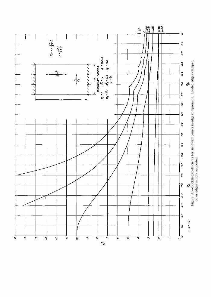
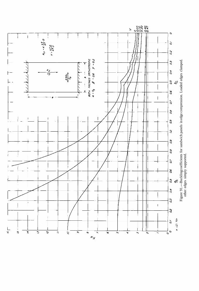
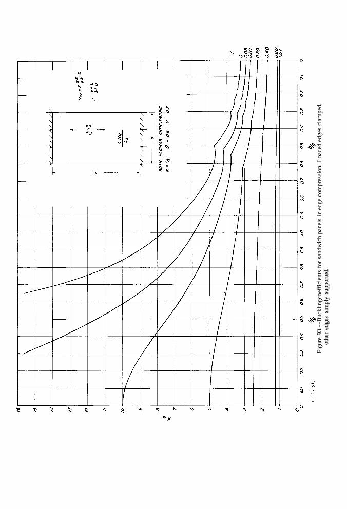
Figu
re 9
5.--
Buc
klin
g coe
ffic
ient
s fo
r sa
ndw
ich
pane
ls i
n ed
ge c
ompr
essi
on. A
ll ed
ges
clam
ped
Figu
re 9
6.--
Buc
klin
g co
effic
ient
s fo
r sa
ndw
ich
pane
ls i
n ed
ge c
ompr
essi
on.
All
edge
s cl
ampe
d.
Figu
re 9
7.--
Buc
klin
g co
effic
ient
s fo
r sa
ndw
ich
pane
ls i
n ed
ge c
ompr
essi
on.
All
edge
s cl
ampe
d.
Figu
re 9
8.--
Buc
klin
g co
effic
ient
s fo
r sa
ndw
ich
pane
ls i
n ed
ge c
ompr
essi
on A
ll ed
ges
clam
ped.

Figu
re 9
9.--
Buc
klin
g co
effic
ient
s fo
r sa
ndw
ich
pane
ls i
n ed
ge c
ompr
essi
on.
All
edge
s cl
ampe
d.

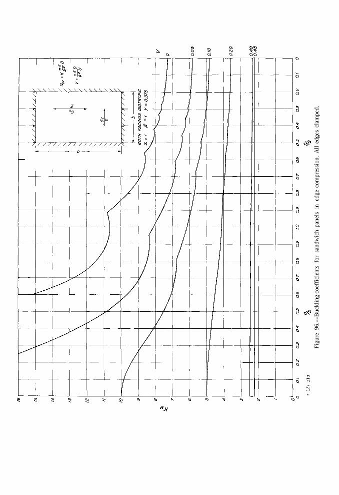
Figu
re 1
00.-
-Buc
klin
g co
effic
ient
s fo
r sa
ndw
ich
pane
ls i
n ed
ge c
ompr
essi
on.
All
edge
s cl
ampe
d.
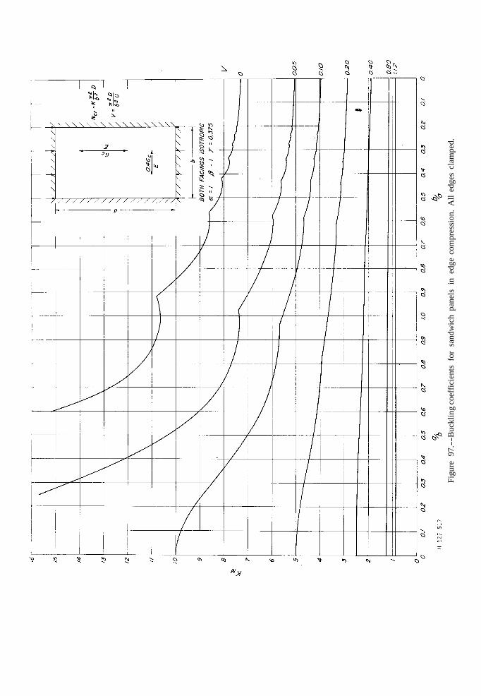
Figu
re 1
01.-
-Buc
klin
g co
effic
ient
s fo
r sa
ndw
ich
pane
ls i
n ed
ge c
ompr
essi
on.
All
edge
s cl
ampe
d.
Figu
re 1
02.-
-Buc
klin
gcoe
ffic
ient
s fo
r sa
ndw
ich
pane
ls in
edg
e co
mpr
essi
on. A
ll ed
ges
clam
ped.

Figu
re 1
03.-
-Buc
klin
g co
effic
ient
s fo
r sa
ndw
ich
pane
ls i
n ed
ge c
ompr
essi
on.
All
edge
s cl
ampe
d.

Figu
re 1
04.-
-Buc
klin
g co
effic
ient
s fo
r sa
ndw
ich
pane
ls i
n ed
ge c
ompr
essi
on.
All
edge
s cl
ampe
d,
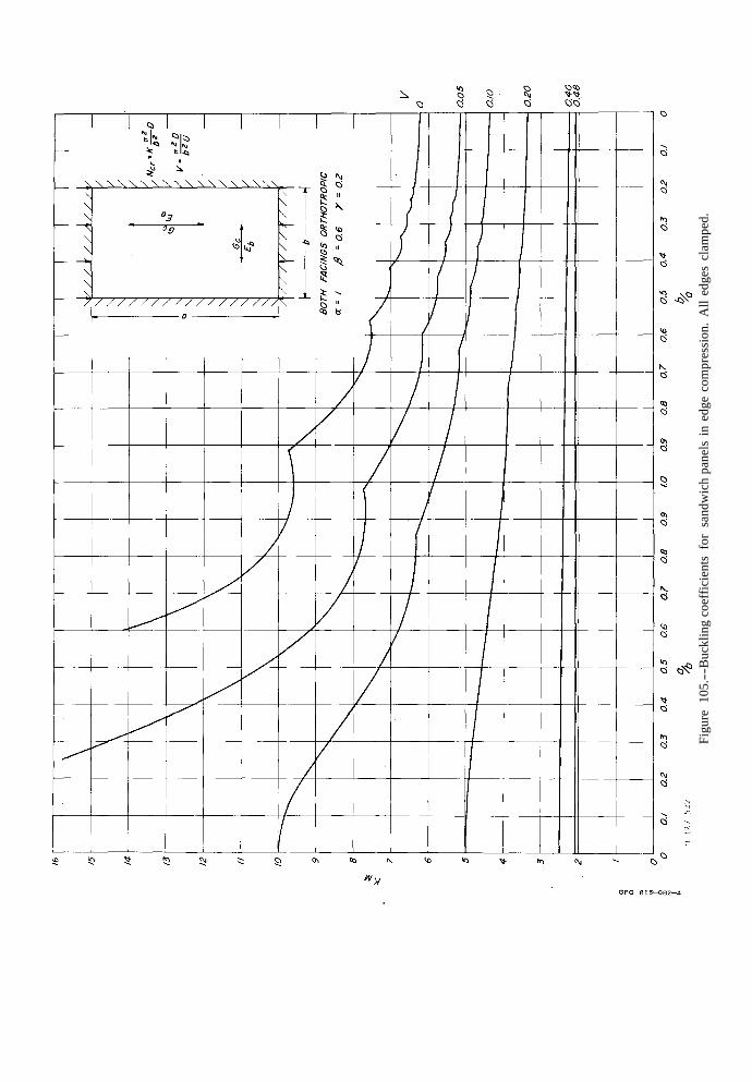
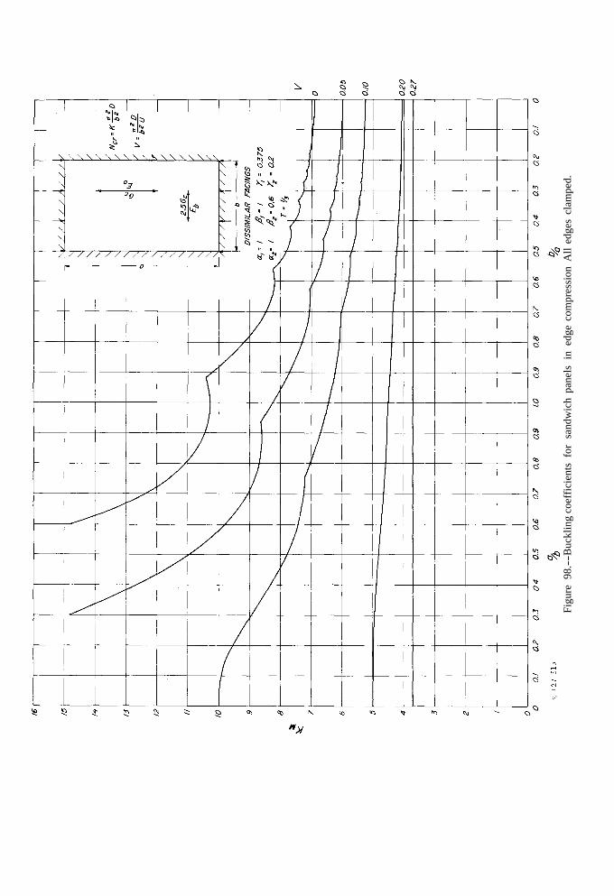
Figu
re 1
05.-
-Buc
klin
g co
effic
ient
s fo
r sa
ndw
ich
pane
ls i
n ed
ge c
ompr
essi
on.
All
edge
s cl
ampe
d.
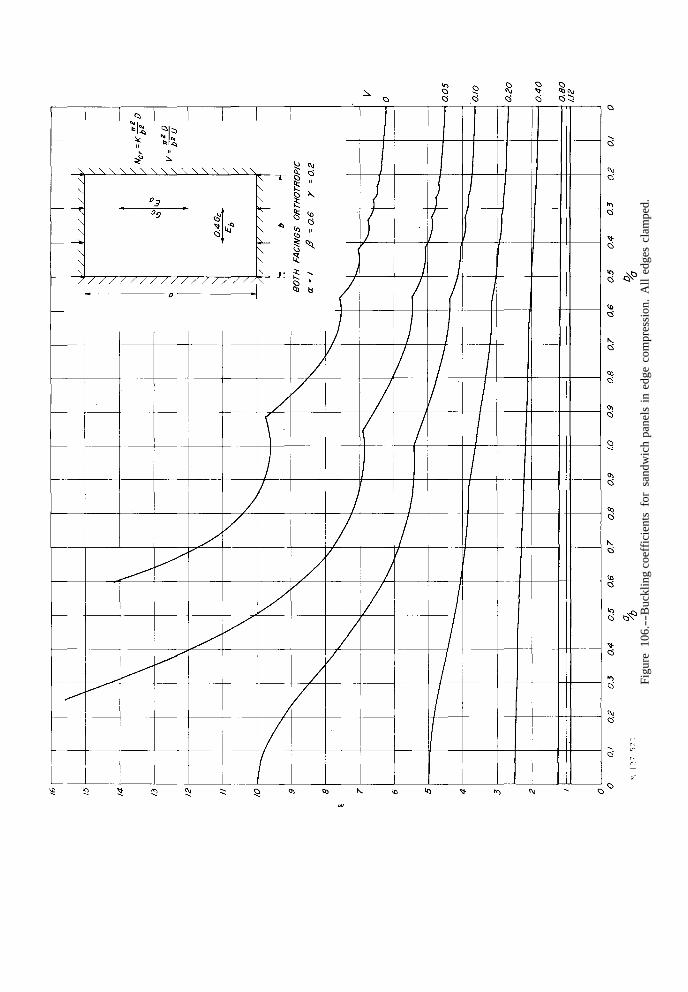
Figu
re 1
06.-
-Buc
klin
g co
effic
ient
s fo
r sa
ndw
ich
pane
ls i
n ed
ge c
ompr
essi
on.
All
edge
s cl
ampe
d.
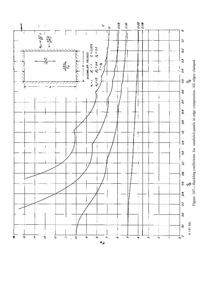
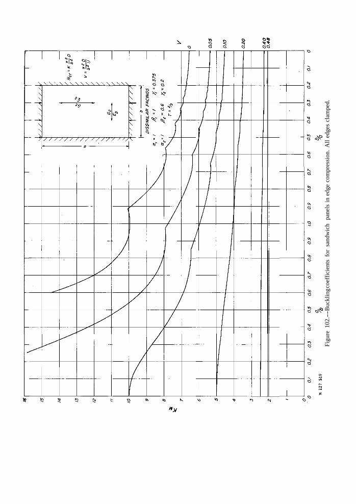
Figu
re 1
07.-
-Buc
klin
g co
effic
ient
s fo
r sa
ndw
ich
pane
ls i
n ed
ge c
ompr
essi
on.
All
edge
s cl
ampe
d.

Figu
re 1
08.-
-Buc
klin
g co
effic
ient
s fo
r sa
ndw
ich
pane
ls i
n ed
ge c
ompr
essi
on.
All
edge
s cl
ampe
d.

Figu
re 1
09.--B
uckl
ing
coef
ficie
nts
for
sand
wic
h pa
nels
in
edge
com
pres
sion
. A
ll ed
ges
clam
ped.

Figu
re 1
10.-
-Buc
klin
g co
effic
ient
s fo
r sa
ndw
ich
pane
ls i
n ed
ge c
ompr
essi
on.
All
edge
s cl
ampe
d.
Figu
re 1
11.-
-Buc
klin
g co
effic
ient
s fo
r sa
ndw
ich
pane
ls i
n ed
ge c
ompr
essi
on.
All
edge
s cl
ampe
d.

Figu
re 1
12.-
-Buc
klin
g co
effic
ient
s fo
r sa
ndw
ich
pane
ls i
n ed
ge c
ompr
essi
on.
All
edge
s cl
ampe
d.

Figu
re 1
13.-
-Buc
klin
g co
effic
ient
s fo
r sa
ndw
ich
pane
ls i
n ed
ge c
ompr
essi
on.
All
edge
s cl
ampe
d.
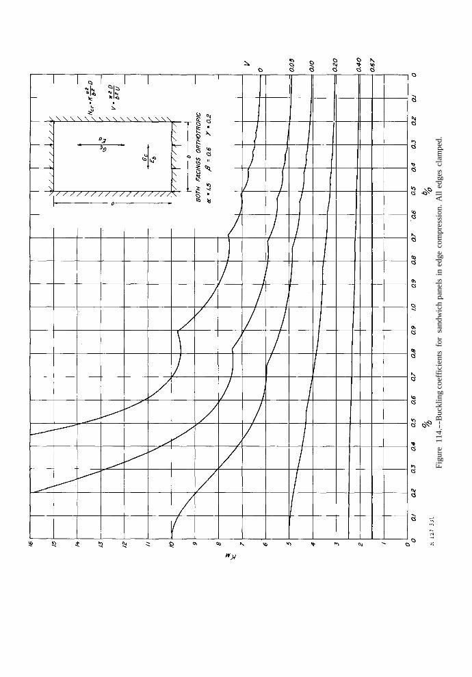
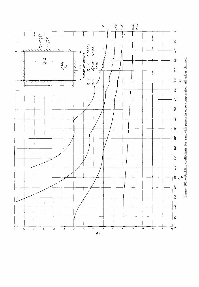
Figu
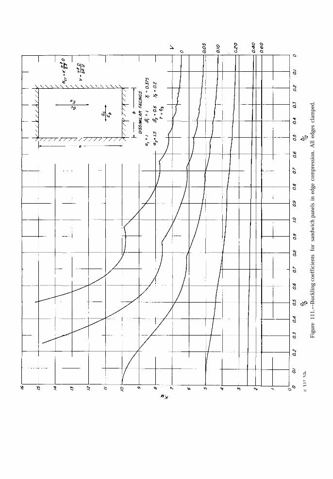
re 1
14.-
-Buc
klin
g co
effic
ient
s fo
r sa
ndw
ich
pane
ls i
n ed
ge c
ompr
essi
on. A
ll ed
ges
clam
ped.
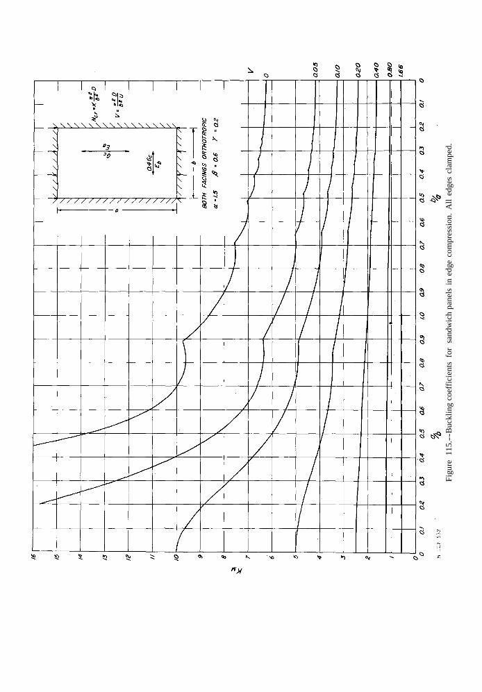
Figu
re 1
15.-
-Buc
klin
g co
effic
ient
s fo
r sa
ndw
ich
pane
ls i
n ed
ge c
ompr
essi
on.
All
edge
s cl
ampe
d.

Figu
re 1
16.-
-Buc
klin
g co
effic
ient
s fo
r sa
ndw
ich
pane
ls i
n ed
ge c
ompr
essi
on.
All
edge
s cl
ampe
d.
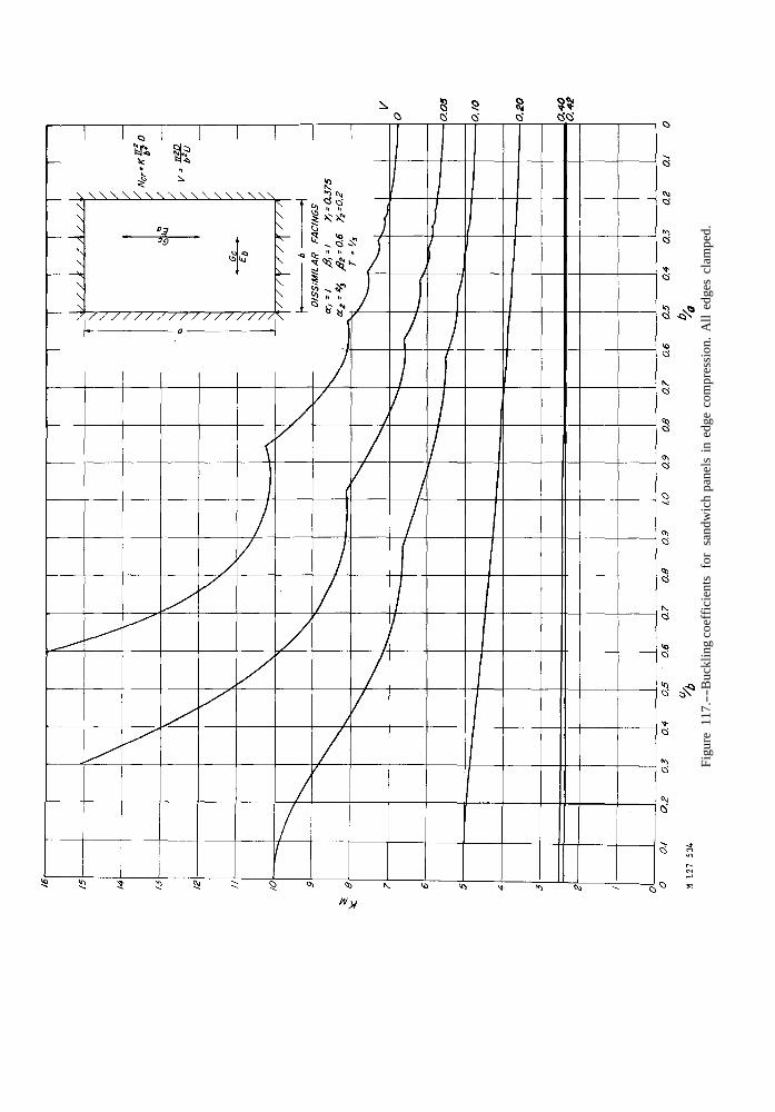
Figu
re 1
17.-
-Buc
klin
g co
effic
ient
s fo
r sa
ndw
ich
pane
ls i
n ed
ge c
ompr
essi
on.
All
edge
s cl
ampe
d.
Figu
re 1
18.--
Buc
klin
g co
effie
ints
for
san
wic
h pa
nels
in
edge
com
pres
sion
. A
ll ed
ges
clam
ped.

Figu
re 1
19.--B
uckl
ing
coef
ficie
nts
for
sand
wic
h pa
nels
in
edge
com
pres
sion
. A
ll ed
ges
clam
ped.

Figu
re 1
20.-
-Buc
klin
g co
effic
ient
s fo
r sa
ndw
ich
pane
ls i
n ed
ge c
ompr
essi
on.
All
edge
s cl
ampe
d.
Figu
re 1
2l--
Buc
klin
g co
effic
ient
s fo
r sa
ndw
ich
pane
ls i
n ed
ge c
ompr
essi
on A
ll ed
ges
clam
ped.
Figu
re 1
22.-
-Buc
klin
g co
effic
ient
s fo
r sa
ndw
ich
pane
ls i
n ed
ge c
ompr
essi
on.
All
edge
s cl
ampe
d.

Figu
re 1
23.--
Buc
klin
g co
effic
ient
for
san
dwic
h pa
nels
in
edge
com
pres
sion
. A
ll ed
ges
clam
ple.

Figu
re 1
24.--
Buc
klin
g co
effic
ient
s fo
r sa
ndw
ich
pane
ls i
n ed
ge c
ompr
essi
on A
ll ed
ges
clam
ped,
Figure 125.--Values of K1 and K2 , (n = 1), for sandwich panels with all edges clamped. β1 = 1,
λ 1
= 3/8. β2
= 0.6, λ 2
= 0.2.
GPO 815-082-2

PUBLICATION LISTS ISSUED BY THE
FOREST PRODUCTS LABORATORY
The following lists of publications deal with investigative projects of the Forest Products Laboratory or relate to special interest groups and are available upon request:
Box, Crate, and Packaging Data
Chemistry of Wood
Drying of Wood
Fire Protection
Fungus and Insect Defects in Forest Products
Glue and Plywood
Growth, Structure, and Identification of Wood
Furniture Manufacturers, Woodworkers, and Teachers of Woodshop Practice
Logging, Milling, and Utilization of Timber Products
Mechanical Properties of Timber
Pulp and Paper
Structural Sandwich, Plastic Laminates, and Wood-Base Components
Thermal Properties of Wood
Wood Finishing Subjects.
Wood Preservation
Architects, Builders, Engineers, and Retail Lumbermen
Note: Since Forest Products Laboratory publications are so varied in subject matter, no single catalog of titles is issued. Instead, a listing is made for each area of Laboratory research. Twice a year, December 31 and June 30, a list is compiled showing new reports for the previous 6 months. This is the only item sent regularly to the Laboratory’s mailing roster, and it serves to keep current the various subject matter listings. Names may be added to the mailing roster upon request.