Budget Constraint,Preferences and Utility

Varian: Intermediate Microeconomics, 8e, Chapters 2, 3 and 4

() 1 / 53

Consumer Theory

Consumers choose the best bundles of goods they can afford.

• This is virtually the entire theory in a nutshell.• But this theory has many surprising consequences.

Two parts to consumer theory

• “can afford” – budget constraint• “best” – according to consumers’ preferences

() 2 / 53

Consumer Theory (cont´d)

What do we want to do with the theory?• Test it. See if it is adequate to describe consumer behavior.• Predict how behavior changes as economic environment changes.• Use observed behavior to estimate underlying values.

These values can be used for• cost-benefit analysis,• predicting impact of some policy.

() 3 / 53

Budget Constraint

The first part of the lecture explains• what is the budget constraint and

the budget line,• how changes in income and prices

affect the budget line,• how taxes, subsidies and rationing

affect the budget line.

() 4 / 53

Consumption Bundle

For goods 1 and 2, the consumption bundle (x1, x2) shows how muchof each good is consumed.

Suppose that we can observe• the prices of the two goods (p1, p2)• and the amount of money the consumer has to spend m

(income).

The budget constraint can be written as p1x1 + p2x2 ≤ m.

The affordable consumption bundles are bundles that don’t cost morethan income.

The set of affordable consumption bundles is budget set of theconsumer.

() 5 / 53

Two Goods

Theory works with more than two goods, butcan’t draw pictures.

We often think of good 2 (say) as acomposite good, representing money tospend on other goods.

Budget constraint becomes p1x1 + x2 ≤ m.

Money spent on good 1 (p1x1) plus the moneyspent on good 2 (x2) has to be less than orequal to the available income (m).

() 6 / 53

Budget Line

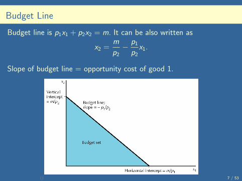
Budget line is p1x1 + p2x2 = m. It can be also written as

x2 =mp2− p1

p2x1.

Slope of budget line = opportunity cost of good 1.

() 7 / 53

Change in Income

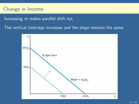
Increasing m makes parallel shift out.

The vertical intercept increases and the slope remains the same.

() 8 / 53

Change in One Price

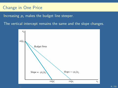
Increasing p1 makes the budget line steeper.

The vertical intercept remains the same and the slope changes.

() 9 / 53

Changes in More Variables

Multiplying all prices by t is just like dividing income by t:

tp1x1 + tp2x2 = m ⇐⇒ p1x1 + p2x2 =mt.

Multiplying all prices and income by t doesn’t change budget line:

tp1x1 + tp2x2 = tm ⇐⇒ p1x1 + p2x2 = m.

A perfectly balanced inflation doesn’t change consumptionpossibilities.

() 10 / 53

Numeraire

We can arbitrarily assign one price or income a value of 1 and adjustthe other variables so as to describe the same budget set.

Budget line: p1x1 + p2x2 = mThe same budget line for p2 = 1:

p1p2

x1 + x2 =mp2.

The same budget line for m = 1:p1m

x1 +p2m

x2 = 1.

The price adjusted to 1 is called the numeraire price.

Useful when measuring relative prices; e.g. English pounds per dollar,1987 dollars versus 1974 dollars, etc.

() 11 / 53

Taxes

Three types of taxes:• quantity tax – consumer pays amount t for each unit she

purchases.→ Price of good 1 increases to p1 + t.

• value tax (or ad valorem tax) – consumer pays a proportion ofthe price τ .→ Price of good 1 increases to p1 + τp1 = (1 + τ)p1.

• lump-sum tax – amount of tax is independent of the consumer’schoices.→ The income of consumer decreases by the amount of the tax.

() 12 / 53

Subsidies

Subsidies – opposite effect than the taxes• quantity subsidy of s on good 1→ Price price of good 1 decreases to p1 − s.

• ad valorem subsidy at a rate of σ on good 1→ Price price of good 1 decreases to p1 − σp1 = (1− σ)p1.

• lump-sum subsidy→ The income increases by the amount of the subsidy.

() 13 / 53

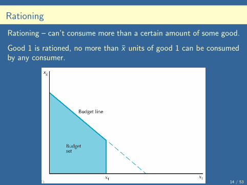
Rationing

Rationing – can’t consume more than a certain amount of some good.

Good 1 is rationed, no more than x̄ units of good 1 can be consumedby any consumer.

() 14 / 53

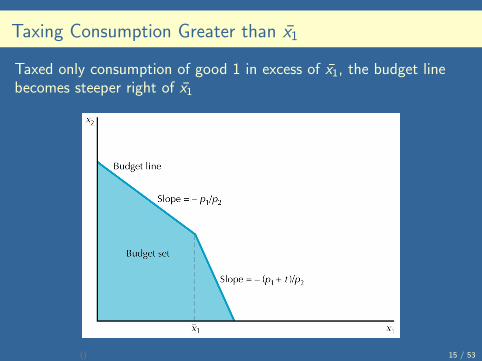
Taxing Consumption Greater than x̄1

Taxed only consumption of good 1 in excess of x̄1, the budget linebecomes steeper right of x̄1

() 15 / 53

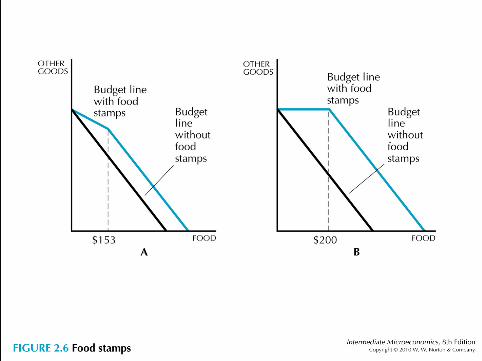
The Food Stamp Program

Before 1979 was an ad valorem subsidy on food• paid a certain amount of money to get food stamps which were

worth more than they cost• some rationing component — could only buy a maximum

amount of food stamps

After 1979 got a straight lump-sum grant of food coupons. Not thesame as a pure lump-sum grant since could only spend the couponson food.

() 16 / 53

() 17 / 53

Summary

• The budget set consists of bundles of goodsthat the consumer can afford at given pricesand income. Typically assume only 2 goods –one of the goods might be composite good.

• The budget line can be written asp1x1 + p2x2 = m.

• Increasing income shifts the budget lineoutward. Increasing price of one good changesthe slope of the budget line.

• Taxes, subsidies, and rationing change theposition and slope of the budget line.

() 18 / 53

Preferences

The second part of the lecture explains• what are consumer’s preferences,• what properties have well-behaved

preferences,• what is marginal rate of

substitution.

() 19 / 53

Preferences - Introduction

Economic model of consumer behavior – peoplechoose the best things they can afford• up to now, we clarified “can afford”• next, we deal with “best things”

Several observations about optimal choice frommovements of budget lines• perfectly balanced inflation doesn’t change

anybody’s optimal choice• after a rise of income, the same choices are

available – consumer must be at least as well ofas before

() 20 / 53

Preferences

Preferences are relationships between bundles.• If a consumer chooses bundle (x1, x2) when (y1, y2) is available,

then it is natural to say that bundle (x1, x2) is preferred to(y1, y2) by this consumer.

• Preferences have to do with the entire bundle of goods, not withindividual goods.

Notation• (x1, x2) � (y1, y2) means the x-bundle is strictly preferred to the

y-bundle.• (x1, x2) ∼ (y1, y2) means that the x-bundle is regarded as

indifferent to the y-bundle.• (x1, x2) � (y1, y2) means the x-bundle is at least as good as

(or weakly preferred) the y-bundle.() 21 / 53

Assumptions about Preferences

Assumptions about “consistency” of consumers’ preferences:• Completeness — any two bundles can be compared:

(x1, x2) � (y1, y2), or (x1, x2) � (y1, y2), or both• Reflexivity — any bundle is at least as good as itself:

(x1, x2) � (x1, x2)• Transitivity — if the bundle X is at least as good as Y and Y

at least as good as Z , then X is at least as good as Z :If (x1, x2) � (y1, y2), and (y1, y2) � (z1, z2), then(x1, x2) � (z1, z2)

Transitivity necessary for theory of optimal choice. Otherwise, therecould be a set of bundles for which there is no best choice.

() 22 / 53

Indifference Curves

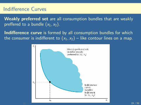
Weakly preferred set are all consumption bundles that are weaklypreffered to a bundle (x1, x2).

Indifference curve is formed by all consumption bundles for whichthe consumer is indifferent to (x1, x2) – like contour lines on a map.

() 23 / 53

Indifference Curves (cont’d)

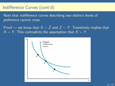
Note that indifference curves describing two distinct levels ofpreference cannot cross.

Proof — we know that X ∼ Z and Z ∼ Y . Transitivity implies thatX ∼ Y . This contradicts the assumption that X � Y .

() 24 / 53

Examples: Perfect Substitutes

Perfect substitutes have constant rate of trade-off between the twogoods; constant slope of the indifference curve (not necessarily −1).

E.g. red pencils and blue pencils; pints and quarts.

() 25 / 53

Examples: Perfect Complements

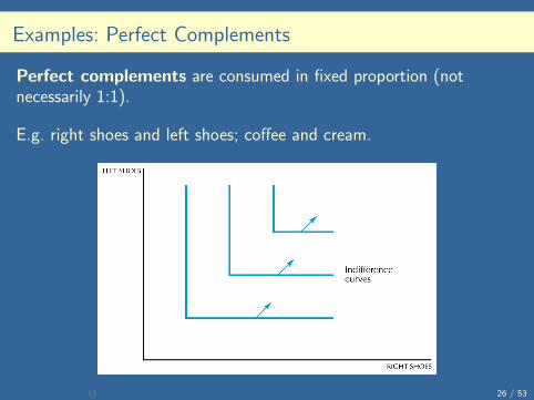
Perfect complements are consumed in fixed proportion (notnecessarily 1:1).

E.g. right shoes and left shoes; coffee and cream.

() 26 / 53

Examples: Bad Good

A bad is a commodity that the consumer doesn’t like.

Suppose consumer is doesn’t like anchovies and likes pepperoni.

() 27 / 53

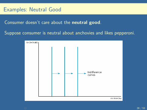
Examples: Neutral Good

Consumer doesn’t care about the neutral good.

Suppose consumer is neutral about anchovies and likes pepperoni.

() 28 / 53

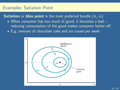
Examples: Satiation Point

Satiation or bliss point is the most preferred bundle (x̄1, x̄2)• When consumer has too much of good, it becomes a bad –

reducing consumption of the good makes consumer better off.• E.g. amount of chocolate cake and ice cream per week

() 29 / 53

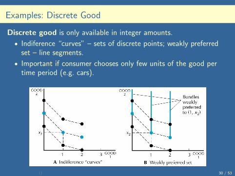
Examples: Discrete Good

Discrete good is only available in integer amounts.• Indiference “curves” – sets of discrete points; weakly preferred

set – line segments.• Important if consumer chooses only few units of the good per

time period (e.g. cars).

() 30 / 53

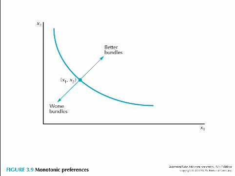
Well-Behaved Preferences

Monotonicity – more is better (we have only goods, not bads) =⇒indifference curves have negative slope (see Figure 3.9):If (y1, y2) has at least as much of both goods as (x1, x2) and more ofone, then (y1, y2) � (x1, x2).

Convexity – averages are preferred to extremes =⇒ slope getsflatter as you move further to right (see Figure 3.10):If (x1, x2) ∼ (y1, y2), then (tx1 + (1− t)y1, tx2 + (1− t)y2) � (x1, x2)for all 0 ≤ t ≤ 1• non convex preferences – olives and ice cream• strict convexity – If the bundles (x1, x2) ∼ (y1, y2), then

(tx1 + (1− t)y1, tx2 + (1− t)y2) � (x1, x2) for all 0 ≤ t ≤ 1

() 31 / 53

() 32 / 53

() 33 / 53

Marginal Rate of Substitution

Marginal rate of substitution (MRS) is the slope of theindifference curve: MRS = ∆x2/∆x1 = dx2/dx1.

Sign problem — natural sign is negative, since indifference curves willgenerally have negative slope.

() 34 / 53

Marginal Rate of Substitution (cont’d)

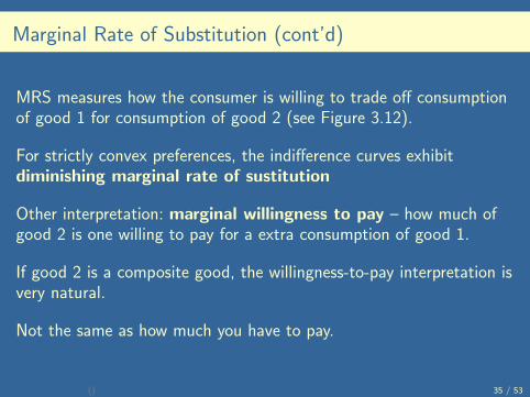
MRS measures how the consumer is willing to trade off consumptionof good 1 for consumption of good 2 (see Figure 3.12).

For strictly convex preferences, the indifference curves exhibitdiminishing marginal rate of sustitution

Other interpretation: marginal willingness to pay – how much ofgood 2 is one willing to pay for a extra consumption of good 1.

If good 2 is a composite good, the willingness-to-pay interpretation isvery natural.

Not the same as how much you have to pay.

() 35 / 53

() 36 / 53

Example: Slope of the Indifference Curve

1) Calculate the slope of the indifference curve x2 = 4/x1 at the point(x1, x2) = (2, 2).

Slope of the indifference curve = MRS =dx2dx1

=−4x21

= −1.

2) Calculate the slope of the indifference curve x2 = 10− 6√

x1 at thepoint (x1, x2) = (4, 5).

Slope of the indifference curve = MRS =dx2dx1

=−3√

x1=−32.

() 37 / 53

Summary

• Economists assume that a consumer can rankconsumption bundles. The ranking describesthe consumer’s preferences.

• The preferences are assumed to be complete,reflexive and transitive.

• Well-behaved preferences are monotonic andconvex.

• MRS measures the slope of the indifferencecurve. MRS can be interpreted as how much ofgood 2 is one willing to pay for an extraconsumption of good 1.

() 38 / 53

Utility

The third part of the lectureexplains• what is utility,• what is a utility function,• what is a monotonic

tranformation of a utilityfunction,

• how can we use utilityfunction to calculate MRS.

() 39 / 53

Utility

Two ways of viewing utility:

Old way - measures how “satisfied” you are(cardinal utility)• not operational• many other problems

New way - summarizes preferences, only theordering of bundles counts (ordinal utility)• operational• gives a complete theory of demand

() 40 / 53

Ordinal Utility

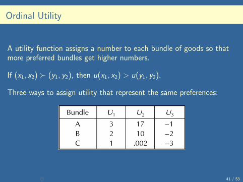
A utility function assigns a number to each bundle of goods so thatmore preferred bundles get higher numbers.

If (x1, x2) � (y1, y2), then u(x1, x2) > u(y1, y2).

Three ways to assign utility that represent the same preferences:

() 41 / 53

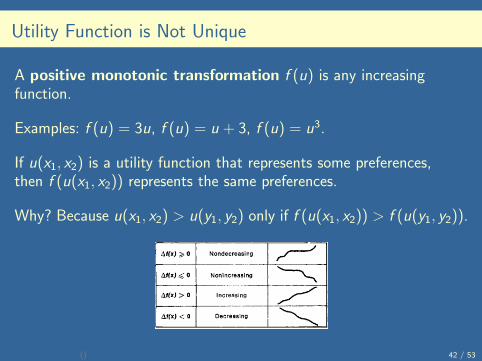
Utility Function is Not Unique

A positive monotonic transformation f (u) is any increasingfunction.

Examples: f (u) = 3u, f (u) = u + 3, f (u) = u3.

If u(x1, x2) is a utility function that represents some preferences,then f (u(x1, x2)) represents the same preferences.

Why? Because u(x1, x2) > u(y1, y2) only if f (u(x1, x2)) > f (u(y1, y2)).

() 42 / 53

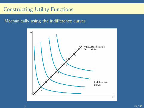
Constructing Utility Functions

Mechanically using the indifference curves.

() 43 / 53

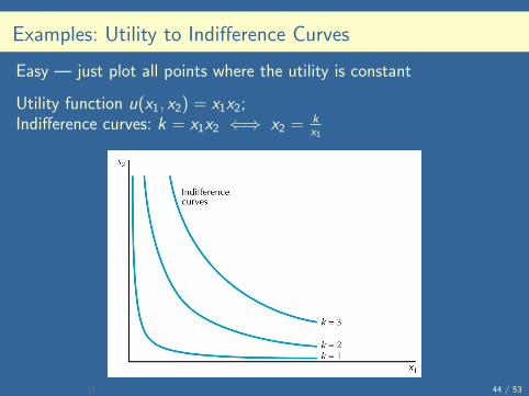
Examples: Utility to Indifference Curves

Easy — just plot all points where the utility is constant

Utility function u(x1, x2) = x1x2;Indifference curves: k = x1x2 ⇐⇒ x2 = k

x1

() 44 / 53

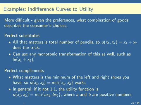
Examples: Indifference Curves to Utility

More difficult - given the preferences, what combination of goodsdescribes the consumer’s choices.

Perfect substitutes• All that matters is total number of pencils, so u(x1, x2) = x1 + x2

does the trick.• Can use any monotonic transformation of this as well, such as

ln(x1 + x2).

Perfect complements• What matters is the minimum of the left and right shoes you

have, so u(x1, x2) = min{x1, x2} works.• In general, if it not 1:1, the utility function is

u(x1, x2) = min{ax1, bx2}, where a and b are positive numbers.

() 45 / 53

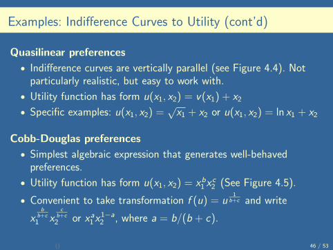
Examples: Indifference Curves to Utility (cont’d)

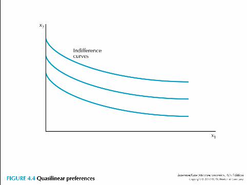
Quasilinear preferences• Indifference curves are vertically parallel (see Figure 4.4). Not

particularly realistic, but easy to work with.• Utility function has form u(x1, x2) = v(x1) + x2• Specific examples: u(x1, x2) =

√x1 + x2 or u(x1, x2) = ln x1 + x2

Cobb-Douglas preferences• Simplest algebraic expression that generates well-behaved

preferences.• Utility function has form u(x1, x2) = xb1 xc2 (See Figure 4.5).

• Convenient to take transformation f (u) = u1b+c and write

xbb+c1 x

cb+c2 or xa1x1−a2 , where a = b/(b + c).

() 46 / 53

() 47 / 53

() 48 / 53

Marginal Utility

Marginal utility (MU) is extra utility from some extra consumptionof one of the goods, holding the other good fixed.

A partial derivative – this just means that you look at the derivativeof u(x1, x2) keeping x2 fixed — treating it like a constant.Examples:• if u(x1, x2) = x1 + x2, then MU1 = ∂u/∂x1 = 1• if u(x1, x2) = xa1x1−a2 , then MU1 = ∂u/∂x1 = axa−11 x1−a2

Note that marginal utility depends on which utility function youchoose to represent preferences.• If you multiply utility 2x, you multiply marginal utility 2x =⇒

it is not an operational concept.• However, MU is closely related to MRS , which is an operational

concept.() 49 / 53

Relationship between MU and MRS

An indifference curve u(x1, x2) = k , where k is a constant.

We want to measure slope of indifference curve, the MRS.

So consider a change (∆x1, ∆x2) that keeps utility constant. Then,

MU1∆x1 + MU2∆x2 = 0

∂u∂x1

∆x1 +∂u∂x2

∆x2 = 0.

Hence,∆x2∆x1

= −MU1MU2

.

So we can compute MRS from knowing the utility function.() 50 / 53

Example: Utility for Commuting

Question: Take a bus or take a car to work?

Each way of transport represents bundle ofdifferent characteristics: Let x1 be the time oftaking a car, y1 be the time of taking a bus.Let x2 be cost of car, etc.

Suppose utility function takes linear formU(x1, ..., xn) = β1x1 + ... + βnxn.

We can observe a number of choices and usestatistical tech- niques to estimate theparameters βi that best describe choices.

() 51 / 53

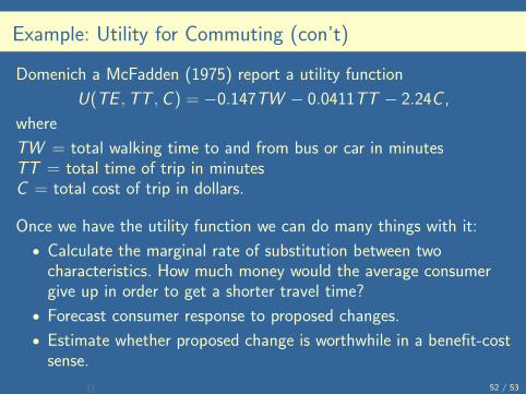
Example: Utility for Commuting (con’t)

Domenich a McFadden (1975) report a utility functionU(TE ,TT ,C ) = −0.147TW − 0.0411TT − 2.24C ,

whereTW = total walking time to and from bus or car in minutesTT = total time of trip in minutesC = total cost of trip in dollars.

Once we have the utility function we can do many things with it:• Calculate the marginal rate of substitution between two

characteristics. How much money would the average consumergive up in order to get a shorter travel time?

• Forecast consumer response to proposed changes.• Estimate whether proposed change is worthwhile in a benefit-cost

sense.() 52 / 53

Summary

• A utility function is a way to represent apreference ordering. The numbersassigned to different utility levels have nointrinsic meaning.

• Any monotonic transformation of a utilityfunction will represent the samepreferences.

• The marginal rate of substitution is equalto MRS = ∆x2/∆x1 = −MU1/MU2.

() 53 / 53